Embed Size (px)
Citation preview
PROBLEMS ON THE GEOMETRIC FUNCTIONTHEORY IN SEVERAL COMPLEX VARIABLES AND
COMPLEX GEOMETRY
BY YUAN YUAN
A dissertation submitted to the
Graduate School—New Brunswick
Rutgers, The State University of New Jersey
in partial fulfillment of the requirements
for the degree of
Doctor of Philosophy
Graduate Program in Mathematics
Written under the direction of
Prof. Xiaojun Huang(advisor) and Prof. Jian Song(co-advisor)
and approved by
New Brunswick, New Jersey
October, 2010
ABSTRACT OF THE DISSERTATION
Problems on the geometric function theory in several
complex variables and complex geometry
by Yuan Yuan
Dissertation Director: Prof. Xiaojun Huang(advisor) and Prof. Jian
Song(co-advisor)
The thesis consists of two parts. In the first part, we study the rigidity for the local
holomorphic isometric embeddings. On the one hand, we prove the total geodesy for
the local holomorphic conformal embedding from the unit ball of complex dimension
at least 2 to the product of unit balls and hence the rigidity for the local holomorphic
isometry is the natural corollary. Before obtaining the total geodesy, the algebraic
extension theorem is derived following the idea in [MN] by considering the sphere bundle
of the source and target domains. When conformal factors are not constant, we twist
the sphere bundle to gain the pseudoconvexity. Then the algebraicity follows from
the algebraicity theorem of Huang in the CR geometry. Different from the argument
in the earlier works, the total geodesy of each factor does not directly follow from
the properness because the codimension is arbitrary. By analyzing the real analytic
subvariety carefully, we conclude that the factor is either a proper holomorphic rational
map or a constant map. Lastly the total geodesy follows from a linearity criterion of
Huang. On the other hand, we also derive the total geodesy for the local holomorphic
isometries from the projective space to the product of projective spaces.
In the second part, we give a proof for the convergence of a modified Kahler-Ricci
ii
flow. The flow is defined by Zhang on Kahler manifolds while the Kahler class along
the evolution is varying. When the limit cohomology class is semi-positive, big and
integer, the convergence of the flow is conjectured by Zhang and we confirm it by
using the monotonicity of some energy functional. When the limit class is Kahler,
the convergence is proven by Zhang and we give an alternative proof by also using
the energy functional. As a corollary, the convergence provides the solution to the
degenerate Monge-Ampere equation on the Calabi-Yau manifold. Meanwhile we take
the opportunity to describe the Kahler-Ricci flow on singular varieties.
iii
Acknowledgements
I would like to express my most sincere gratitude to my advisor Professor Xiaojun
Huang, for everything he has done to help me grow up in my academic life. I must
mention that from the very beginning when I was totally lost being a junior graduate
student, he has kept pointing out to me the right direction. During my Ph.D study,
he provided me numerous interesting problems and shared with me his insight and
new ideas to these problems without any reservation. He encouraged me when I was
frustrated and gave me the pressure when I did not do my work well. Last but not
least, the thesis would not be possible without all his help.
I also would like to express the sincere acknowledgements to my co-advisor Professor
Jian Song. Without the numerous discussions and constant support, the second part
of the thesis can not be accomplished.
I would like to thank Professor N. Mok for his very useful suggestions and constant
support. I would like to thank Professor D.H. Phong for his very helpful discussions and
constant encouragement. I benefit greatly from Professor Phong’s seminar in Columbia
University. I also would like to thank Professor G. Tian for the stimulating discussions.
I am indebted to Professor S. Berhanu, Professor S. Chanillo, Professor H. Ja-
cobowitz for their constant support.
I am indebted to Professor S. Fu, Professor S. Greenfield, Professor Z. Han, Professor
S. Li, Professor Y. Li, Professor F. Luo, Professor G. Mendoza, Professor X. Rong and
Professor B. Shiffman for their encouragement and help during my graduate study. I
am also indebted to C. Li, S. Ng, V. Tosatti, T. Yang, W. Yin, X. Yuan, Y. Zhang, Z.
Zhang and many other people for their useful discussions.
I would like to thank all the faculty, staff and my fellow graduate students in the
department of Mathematics at Rutgers for their care and help.
iv

I am very grateful to my parents, grandparents and other family members for their
love and support. I would like to express my gratitude to Lin Chen for everything she
has brought to me.
v

Dedication
This thesis is dedicated to my family.
vi
Table of Contents
Abstract . . . . . . . . . . . . . . . . . . . . . . . . . . . . . . . . . . . . . . . . ii
Acknowledgements . . . . . . . . . . . . . . . . . . . . . . . . . . . . . . . . . iv
Dedication . . . . . . . . . . . . . . . . . . . . . . . . . . . . . . . . . . . . . . . vi
1. Introduction . . . . . . . . . . . . . . . . . . . . . . . . . . . . . . . . . . . 1
1.1. Rigidity for local holomorphic isometric embeddings . . . . . . . . . . . 1
1.2. The Kahler-Ricci flow . . . . . . . . . . . . . . . . . . . . . . . . . . . . 4
2. Rigidity for local holomorphic isometric embeddings . . . . . . . . . . 8
2.1. Rigidity for local holomorphic conformal embeddings from the unit ball
into the product of unit balls . . . . . . . . . . . . . . . . . . . . . . . . 8
2.1.1. Main results . . . . . . . . . . . . . . . . . . . . . . . . . . . . . . 8
2.1.2. Bergman metric and proper rational maps . . . . . . . . . . . . 9
2.1.3. Algebraic extension . . . . . . . . . . . . . . . . . . . . . . . . . 17
2.1.4. Proof of Theorem 2.1.1 . . . . . . . . . . . . . . . . . . . . . . . 20
2.2. Rigidity for local holomorphic isometric embeddings from the projective
space into the product of projective spaces . . . . . . . . . . . . . . . . . 26
3. On the modified Kahler-Ricci flow . . . . . . . . . . . . . . . . . . . . . 32
3.1. Preliminaries . . . . . . . . . . . . . . . . . . . . . . . . . . . . . . . . . 32
3.2. Proof of Theorem 3.1.1 . . . . . . . . . . . . . . . . . . . . . . . . . . . . 37
3.3. Remarks on non-degenerate case . . . . . . . . . . . . . . . . . . . . . . 40
References . . . . . . . . . . . . . . . . . . . . . . . . . . . . . . . . . . . . . . . 45
Vita . . . . . . . . . . . . . . . . . . . . . . . . . . . . . . . . . . . . . . . . . . . 49
vii
1
Chapter 1
Introduction
1.1 Rigidity for local holomorphic isometric embeddings
Various rigidity problems in Several Complex Variables and Complex Geometry are
among the basic problems in the subject. The understanding of these problems is not
only important for the subject itself, but also plays a critical role in the application to
many other research fields of mathematics.
The study of the topic will be focused on the rigidity problem for the local holomor-
phic isometric embeddings between Hermitian symmetric spaces. This type of problems
is initialled in a celebrated paper of Calabi, who first studied the global extension and
Borel type rigidity of a local holomorphic isometric embedding between Kahler man-
ifolds with real analytic metrics [Ca]. Afterwards, there appeared quite a few papers
along these lines of research (see [Um], for instance). In 2004, motivated from the
problems in Arithmetic Algebraic Geometry, Clozel-Ullmo [CU] took up the problem
again by considering the rigidity of local holomorphic isometries from a bounded sym-
metric domain into its product with respect to their Bergman metrics. More precisely,
by reducing the problem to the rigidity problem for local holomorphic isometries, they
proved the algebraic correspondence between such quotients of bounded symmetric do-
mains preserving Bergman metric has to be modular correspondence in the case of (i)
unit disc in the complex plane and (ii) bounded symmetric domains of rank at least 2.
More recently, Mok carried out a systematic study of this problem in a very general
setting. Many deep results have been obtained by Mok and Mok-Ng. (See [Mo1] [Mo3]
[MN] [Ng1-3] and the references therein). For instance, Mok proved the total geodesy
for the local holomorphic isometry between bounded symmetric domains D and Ω when
either (i) rank(D) ≥ 2 or (2) D = Bn and Ω = (Bn)p for n ≥ 2.
2
In the second chapter, we prove the rigidity for local holomorphic conformal em-
beddings between the unit ball and the product of unit balls and as a corollary, obtain
the rigidity for local holomorphic isometric embeddings between such domains. This
theorem appears in [YZ]. (See chapter 2 for relevant notations)
Theorem 1.1.1 Let
F = (F1, . . . , Fm) : (U ⊂ Bn, λ(z, z)ds2n)→ (BN1×· · ·×BNm ,⊕mj=1λj(z, z)ds
2Nj ) (1.1.1)
be a local holomorphic conformal embedding in the sense that
λ(z, z)ds2n =
m∑j=1
λj(z, z)F ∗j (ds2Nj ).
Assume that n ≥ 2 and λ(z, z), λj(z, z) are positive Nash algebraic functions. We then
have, for each j with 1 ≤ j ≤ m, that either Fj is a constant map or Fj extends to a
totally geodesic holomorphic embedding from (Bn, ds2n) into (BNj , ds2
Nj).
When λ(z, z), λj(z, z) are constants, the result is due to Calabi when m = 1 [Ca],
due to Mok [Mo1] [Mo3] when N1 = · · · = Nm, and due to Ng [Ng1] [Ng3] when m = 2
and N1, N2 < 2n. The novelty of our result is that the factor in the target manifold
can be any BN .
Our proof of Theorem 1.1.1 is based on the algebraic extension theorem. In the case
of the conformal embedding, it does not follow from [Mo2] directly. Following [MN],
we try to use the unit sphere bundle of the corresponding domain and reduce the alge-
braicity to the mapping problem in CR geometry. However, since the pseudoconvexity
is totally lost, we need to twist the sphere bundle to gain the positivity.
To obtain the total geodesy, different from the case considered in [Mo1] [Ng1], the
properness of a factor of F does not imply the linearity of that factor, for the classical
linearity theorem does not hold anymore for proper rational mappings from Bn into
BN with N > 2n − 2. To make up this, we carried out a careful study on the precise
boundary behavior of the Bergman metric pulled back by proper holomorphic maps.
It turns out that the difference of the pull-back Bergman metric of the target space
with the source Bergman metric is smooth up to the boundary and the values on
3
the boundary are closely related to the boundary CR invariants inherited from the
map. Another ingredient in our argument is a careful analysis for the (multiple-valued)
holomorphic continuation of the local holomorphic map. The key for this part is to
analyze the real analytic subvariety where the pull-back of the Bergman metric blows up.
In our proof of Theorem 1.1.1, a major step is to prove that a non-constant component
Fj of F must be proper from Bn into BNj , using the multiple-valued holomorphic
continuation technique. This then reduces the proof of Theorem 1.1.1 to the case
when all components are proper. Unfortunately, due to the non-constancy for the
conformal factors λj(z, z) and λ(z, z), it is not immediate that each component must
also be conformal (and thus must have conformal factor constant) with respect to the
normalized Bergman metric. However, we observe that the blowing-up rate for the
Bergman metric of Bn with n ≥ 2 in the complex normal direction is twice of that
along the complex tangential direction, when approaching the boundary. From this,
we will be able to derive an equation connecting the CR invariants associated from the
map at the boundary of the ball. Lastly, a linearity criterion of Huang in [Hu1] can be
applied to simultaneously conclude the linearity of all components.
Notice that Theorem 1.1.1 fails when n = 1 by Mok [Mo1] and later by Ng [Ng1].
By the previous work of Mok, we have a good understanding for the case when the rank
of source domain is at least 2. Hence, our result provides a fairly complete picture for
such a problem for the non-compact model in the rank one case.
When manifolds are compact Hermitian symmetric spaces, the rigidity property is
unknown even in the case of projective spaces. The following question is the nature
starting problem of the compact case:
Question 1.1.1 Let
F : (U ⊂ Pn, ωn)→ (PN1 × · · · × PNp ,⊕pl=1λlωNl)
be a local holomorphic isometric imbedding with respect to Fubini-Study metrics. How
to classify F?
The global extension of the map F above has been established by Calabi and Mok
[Ca] [Mo3] for some partial cases. Also, we know that the linearity for F fails even when
4
p = 1, for the Veronese imbedding from (Pn, 2ωn) into (Pn(n+3)
2 , ωn(n+3)2
) is an isometry
and of degree 2. However, it is generally believed that a non-constant component of F
is equivalent to the Veronese imbedding of some integer isometric constant.
In chapter 2, we study such problems. More precisely, we prove the following theo-
rem. (See chapter 2 for relevant notations.)
Theorem 1.1.2 Let λl ∈ Q and let
F = (F1, · · · , Fp) : (U ⊂ Pn, ωn)→ (PN1 × · · · × PNp ,⊕pl=1λlωNl)
be a local holomorphic isometric imbedding with respect to Fubini-Study metrics, i.e.
ωn =∑l
λlF∗l ωNl .
Let κ1, · · · , κp ∈ (Z+)p satisfy
(i) Nl ≥Mn,κl for 1 ≤ l ≤ p,
(ii)∑p
l=1 κlλl = 1.
Then the possibility of κ1, · · · , κp gives the classification of F = (F1, · · · , Fp). In par-
ticular, Fl is equivalent to Veronese embedding Vn,κl with isometric constant κl modular
Isom(PNl , ωNl) and Fl is a constant map if κl = 0.
1.2 The Kahler-Ricci flow
The Ricci flow was introduced by Richard Hamilton [H] on Riemannian manifolds to
study the deformation of metrics. Its analogue in Kahler geometry, the Kaher-Ricci
flow, has been intensively studied in recent years. It turns out to be a powerful method
for studying canonical metrics on Kahler manifolds. (See, for instance, the papers [Cao]
[CT] [Pe] [PS] [PSSW] [ST1] [ST2] [TZhu] and the references therein.)
In a recent paper [Z3], a modified Kahler-Ricci flow was defined by Zhang by allowing
the cohomology class to vary artificially. Consider the following Monge-Ampere flow
(see Chapter 3 for relevant notations):
5
∂∂tϕ = log (ωt+
√−1∂∂ϕ)n
Ω ,
ϕ(0, ·) = 0.
(1.2.1)
Then the evolution for the corresponding Kahler metric is given by:
∂∂t ωt = −Ric(ωt) +Ric(Ω)− e−tχ,
ωt(0, ·) = ω0.
(1.2.2)
As pointed out by Zhang, the motivation is to apply the geometric flow technique
to study the complex Monge-Ampere equation:
(ω∞ +√−1∂∂ψ)n = Ω. (1.2.3)
This equation has already been intensively studied very recently by using the pluri-
potential theory developed by Bedford-Taylor, Demailly, Ko lodziej et al. When Ω is a
smooth volume form and [ω∞] is Kahler, the equation is solved by Yau in his solution to
the celebrated Calabi conjecture using the continuity method [Y1]. When Ω is Lp with
respect to another smooth reference volume form and [ω∞] is Kahler, the continuous
solution is obtained by Ko lodziej [K1]. Later on, the bounded solution is obtained in
[Z2] and [EGZ] independently, generalizing Ko lodziej’s theorem to the case when [ω∞]
is big and semi-positive, and Ω is also Lp. On the other hand, as an interesting question,
equation (1.2.3) is also studied on symplectic manifolds by Weinkove [We].
In the case of the unnormalized Kahler-Ricci flow, the evolution for the cohomology
class of the metric is in the direction of the canonical class of the manifold. While in the
case of (1.2.2), one can try to deform any initial metric class to an arbitrary desirable
limit class. In particular, on Calabi-Yau manifolds, the flow (1.2.2) converges to a Ricci
flat metric, if Ω is a Calabi-Yau volume form, with the initial metric also Ricci flat in
a different cohomology class [Z3].
The existence and convergence of the solution are proved by Zhang [Z3] for the
above flow in the case when [ω∞] is Kahler, which corresponds to the case considered
6
by Cao in the classical Kahler-Ricci flow [Cao]. When [ω∞] is big, (1.2.2) may produce
singularities at finite time T < +∞. In this case, the local C∞ convergence of the flow
away from a proper analytic subvariety of X was obtained in [Z3] under the further
assumption that [ωT ] is semi-positive. When [ω∞] is semi-positive and big, Zhang also
obtained the long time existence of the solution as well as important estimates and
conjectured the convergence even in this more general setting. In Chapter 3, we give a
proof to this conjecture.
Theorem 1.2.1 Let X be a Kahler manifold with a Kahler metric ω0. Suppose that
[ω∞] ∈ H1,1(X,C)∩H2(X,Z) is semi-positive and big. Then along the modified Kahler-
Ricci flow (1.2.2), ωt converges weakly in the sense of currents and converges locally
in C∞-norm away from a proper analytic subvariety of X to the unique solution of the
degenerate Monge-Ampere equation (1.2.3).
Corollary 1.2.1 When X is a Calabi-Yau manifold and Ω is a Calabi-Yau volume
form, ωt converges to a singular Calabi-Yau metric.
Singular Calabi-Yau metrics are already obtained in [EGZ] on normal Calabi-Yau
Kahler spaces, and obtained by Song-Tian [ST2] and Tosatti [To] independently in the
degenerate class on algebraic Calabi-Yau manifolds. The uniqueness of the solution
to the equation (1.2.3) in the degenerate case when [ω∞] is semi-positive and big has
been studied in [EGZ] [Z2] [DZ] etc. In particular, a stability theorem is proved in [DZ]
which immediately implies the uniqueness. In [To], Tosatti studied the deformation for
a family of Ricci flat Kahler metrics, whose cohomology classes are approaching a big
and nef class. Here our deformation (equation (1.2.2)) gives different paths connecting
non-singular and singular Calabi-Yau metrics.
The Kahler-Ricci flow on singular algebraic varieties is defined by Song-Tian [ST3] to
study the singularities and surgeries. Starting with the singular and degenerate initial
data on general algebraic varieties, the existence and uniqueness of the Kahler-Ricci
flow is derived in [ST3]. We then prove the convergence of the Kahler-Ricci flow on
projective Calabi-Yau varieties. As a corollary, we also obtain the singular Calabi-Yau
metric on such varieties. This result appears in [SY].
7
Theorem 1.2.2 Let X ⊂ PN be a projective Calabi-Yau variety with log terminal
singularities. Let ω0 be the Kahler metric equivalent to the pull-back of the Fubini-
Study metric on PN . Then the unnormalized weak Kahler-Ricci flow
∂∂tω = −Ric(ω),
ω(0, ·) = ω0 on X
(1.2.4)
has a unique weak solution ω(t, ·) on [0,∞) × X, where ω(t, ·) ∈ C∞([0,∞) × Xreg)
and ω(t, ·) admits a bounded local potenial. Furthermore, ω(t, ·) converges to the unique
singular Ricci-flat Kahler metric ωCY ∈ [ω0] in the sense of currents on X and in
C∞-topology on Xreg = X \Xsing.
8
Chapter 2
Rigidity for local holomorphic isometric embeddings
2.1 Rigidity for local holomorphic conformal embeddings from the
unit ball into the product of unit balls
2.1.1 Main results
Write Bn := z ∈ Cn : |z| < 1 for the unit ball in Cn. Denote by ds2n the normalized
Bergman metric on Bn defined as follows:
ds2n =
∑j,k≤n
1(1− |z|2)2
((1− |z|2)δjk + zjzk
)dzj ⊗ dzk. (2.1.1)
Let U ⊂ Bn be a connected open subset and consider a holomorphic conformal embed-
ding
F = (F1, . . . , Fm) : (U ⊂ Bn, λ(z, z)ds2n)→ (BN1×· · ·×BNm ,⊕mj=1λj(z, z)ds
2Nj ) (2.1.2)
in the sense that λ(z, z)ds2n =
∑mj=1 λj(z, z)F
∗j (ds2
Nj). Here λj(z, z) > 0, λ(z, z) > 0 are
assumed to be positive-valued smooth Nash algebraic functions over Cn. Moreover, for
each j with 1 ≤ j ≤ m, ds2Nj
denotes the corresponding normalized Bergman metric of
BNj and Fj is a holomorphic map from U to BNj . We write Fj = (fj,1, . . . , fj,l, . . . , fj,Nj ),
where fj,l is the l-th component of Fj . In this section, we prove the following rigidity
theorem:
Theorem 2.1.1 Suppose n ≥ 2. Under the above notation and assumption, we then
have, for each j with 1 ≤ j ≤ m, that either Fj is a constant map or Fj extends to a
totally geodesic holomorphic embedding from (Bn, ds2n) into (BNj , ds2
Nj). Moreover, we
have the following identity ∑Fj is not a constant
λj(z, z) = λ(z, z).
9
In particular, when λj(z, z), λ(z, z) are positive constant functions, we have the
following rigidity result for local isometric embeddings:
Corollary 2.1.1 Let
F = (F1, . . . , Fm) : (U ⊂ Bn, λds2n)→ (BN1 × · · · × BNm ,⊕mj=1λjds
2Nj ) (2.1.3)
be a local holomorphic isometric embedding in the sense that λds2n =
∑mj=1 λjF
∗j (ds2
Nj).
Assume that n ≥ 2 and λ, λj are positive constants. We then have, for each j with 1 ≤
j ≤ m, that either Fj is a constant map or Fj extends to a totally geodesic holomorphic
embedding from (Bn, ds2n) into (BNj , ds2
Nj). Moreover, we have the following identity
∑Fj is not a constant
λj = λ.
Recall that a function h(z, z) is called a Nash algebraic function over Cn if it is either
constant or if there is an irreducible polynomial P (z, ξ,X) in (z, ξ,X) ∈ Cn × Cn × C
with P (z, z, h(z, z)) ≡ 0 over Cn. We mention that a holomorphic map from Bn into BN
is a totally geodesic embedding with respect to the normalized Bergman metric if and
only if there are a (holomorphic) automorphism σ ∈ Aut(Bn) and an automorphism
τ ∈ Aut(BN ) such that τ F σ(z) ≡ (z, 0).
2.1.2 Bergman metric and proper rational maps
Let Bn and ds2n be the unit ball and its normalized Bergman metric, respectively, as
defined before. Denote by Hn ⊂ Cn the Siegel upper half space. Namely, Hn =
(z, w) ∈ Cn−1 × C : =w − |z|2 > 0. Here, for m-tuples a, b, we write dot product
a · b =∑m
j=1 ajbj and |z|2 = z · z. Recall the following Cayley transformation
ρn(z, w) =(
2z1− iw
,1 + iw
1− iw
). (2.1.4)
Then ρn biholomorphically maps Hn to Bn, and biholomorphically maps ∂Hn, the
Heisenberg hypersurface, to ∂Bn\(0, 1). Applying the Cayley transformation, one
10
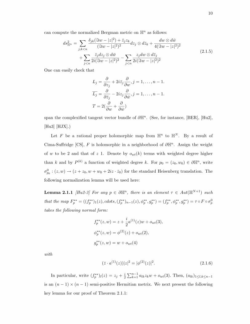
can compute the normalized Bergman metric on Hn as follows:
ds2Hn =
∑j,k<n
δjk(=w − |z|2) + zjzk(=w − |z|2)2
dzj ⊗ dzk +dw ⊗ dw
4(=w − |z|2)2
+∑j<n
zjdzj ⊗ dw2i(=w − |z|2)2
−∑j<n
zjdw ⊗ dzj2i(=w − |z|2)2
(2.1.5)
One can easily check that
Lj =∂
∂zj+ 2izj
∂
∂w, j = 1, . . . , n− 1.
Lj =∂
∂zj− 2izj
∂
∂w, j = 1, . . . , n− 1.
T = 2(∂
∂w+
∂
∂w)
span the complexified tangent vector bundle of ∂Hn. (See, for instance, [BER], [Hu2],
[Hu3] [HJX].)
Let F be a rational proper holomorphic map from Hn to HN . By a result of
Cima-Suffridge [CS], F is holomorphic in a neighborhood of ∂Hn. Assign the weight
of w to be 2 and that of z 1. Denote by owt(k) terms with weighted degree higher
than k and by P (k) a function of weighted degree k. For p0 = (z0, w0) ∈ ∂Hn, write
σ0p0
: (z, w) → (z + z0, w + w0 + 2iz · z0) for the standard Heisenberg translation. The
following normalization lemma will be used here:
Lemma 2.1.1 [Hu2-3] For any p ∈ ∂Hn, there is an element τ ∈ Aut(HN+1) such
that the map F ∗∗p = ((f∗∗p )1(z), cdots, (f∗∗p )n−1(z), φ∗∗p , g∗∗p ) = (f∗∗p , φ
∗∗p , g
∗∗p ) = τ F σ0
p
takes the following normal form:
f∗∗p (z, w) = z +i
2a(1)(z)w + owt(3),
φ∗∗p (z, w) = φ(2)(z) + owt(2),
g∗∗p (z, w) = w + owt(4)
with
(z · a(1)(z))|z|2 = |φ(2)(z)|2. (2.1.6)
In particular, write (f∗∗p )l(z) = zj + i2
∑n−1k=1 alkzkw + owt(3). Then, (alk)1≤l,k≤n−1
is an (n− 1)× (n− 1) semi-positive Hermitian metrix. We next present the following
key lemma for our proof of Theorem 2.1.1:
11
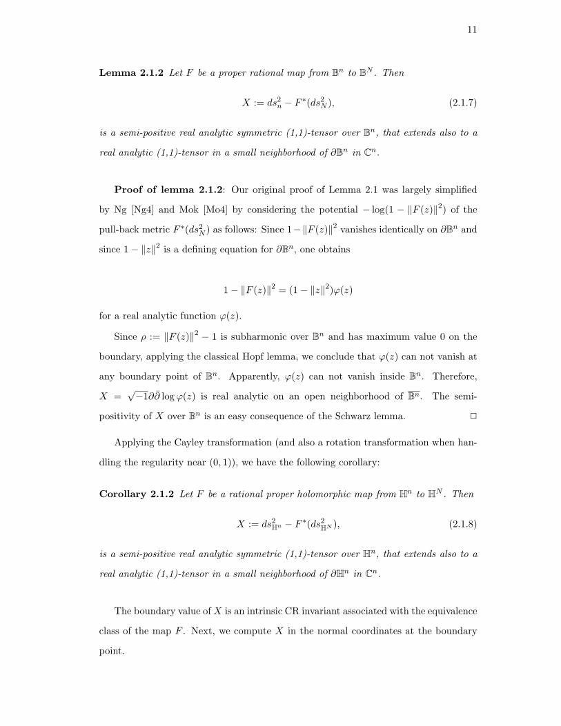
Lemma 2.1.2 Let F be a proper rational map from Bn to BN . Then
X := ds2n − F ∗(ds2
N ), (2.1.7)
is a semi-positive real analytic symmetric (1,1)-tensor over Bn, that extends also to a
real analytic (1,1)-tensor in a small neighborhood of ∂Bn in Cn.
Proof of lemma 2.1.2: Our original proof of Lemma 2.1 was largely simplified
by Ng [Ng4] and Mok [Mo4] by considering the potential − log(1 − ‖F (z)‖2) of the
pull-back metric F ∗(ds2N ) as follows: Since 1−‖F (z)‖2 vanishes identically on ∂Bn and
since 1− ‖z‖2 is a defining equation for ∂Bn, one obtains
1− ‖F (z)‖2 = (1− ‖z‖2)ϕ(z)
for a real analytic function ϕ(z).
Since ρ := ‖F (z)‖2 − 1 is subharmonic over Bn and has maximum value 0 on the
boundary, applying the classical Hopf lemma, we conclude that ϕ(z) can not vanish at
any boundary point of Bn. Apparently, ϕ(z) can not vanish inside Bn. Therefore,
X =√−1∂∂ logϕ(z) is real analytic on an open neighborhood of Bn. The semi-
positivity of X over Bn is an easy consequence of the Schwarz lemma. 2
Applying the Cayley transformation (and also a rotation transformation when han-
dling the regularity near (0, 1)), we have the following corollary:
Corollary 2.1.2 Let F be a rational proper holomorphic map from Hn to HN . Then
X := ds2Hn − F ∗(ds2
HN ), (2.1.8)
is a semi-positive real analytic symmetric (1,1)-tensor over Hn, that extends also to a
real analytic (1,1)-tensor in a small neighborhood of ∂Hn in Cn.
The boundary value of X is an intrinsic CR invariant associated with the equivalence
class of the map F . Next, we compute X in the normal coordinates at the boundary
point.
12
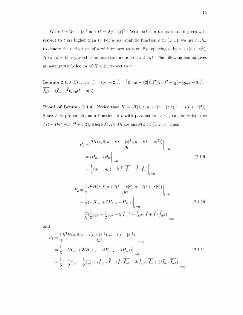
Write t = =w − |z|2 and H = =g − |f |2 . Write o(k) for terms whose degrees with
respect to t are higher than k. For a real analytic function h in (z, w), we use hz, hw
to denote the derivatives of h with respect to z, w. By replacing w by u + i(t + |z|2),
H can also be regarded as an analytic function on z, z, u, t. The following lemma gives
an asymptotic behavior of H with respect to t:
Lemma 2.1.3 H(z, z, u, t) = (gw − 2ifw · ¯f)|t=0t − (2|fw|2)|t=0t
2 + 13(−1
2gw3 + 3ifw ·
fw2 + ifw3 · ¯f)|t=0t
3 + o(3).
Proof of Lemma 2.1.3: Notice that H = H(z, z, u + i(t + |z|2), u − i(t + |z|2)).
Since F is proper, H, as a function of t with parameters z, u, can be written as
P1t+ P2t2 + P3t
3 + o(3), where P1, P2, P3 are analytic in (z, z, u). Then
P1 =∂H(z, z, u+ i(t+ |z|2), u− i(t+ |z|2))
∂t
∣∣∣∣t=0
= iHw − iHw
∣∣∣∣t=0
=12
(gw + gw) + i(f · fw − ¯f · fw)
∣∣∣∣t=0
,
(2.1.9)
P2 =12∂2H(z, z, u+ i(t+ |z|2), u− i(t+ |z|2))
∂t2
∣∣∣∣t=0
=12
(−Hw2 + 2Hww −Hww)∣∣∣∣t=0
=12
(i
2gw2 −
i
2gw2 − 2|fw|2 + fw2 · ¯
f + f · fw2)∣∣∣∣t=0
,
(2.1.10)
and
P3 =16∂3H(z, z, u+ i(t+ |z|2), u− i(t+ |z|2))
∂t3
∣∣∣∣t=0
=16
(−iHw3 + 3iHw2w − 3iHw2w + iHw3)∣∣∣∣t=0
=16
(−12gw3 −
12gw3 + ifw3 · ¯
f − if · fw3 − 3ifw2 · fw + 3ifw · fw2)∣∣∣∣t=0
.
(2.1.11)
13
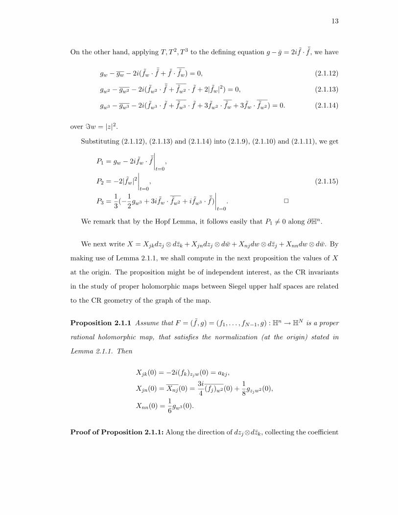
On the other hand, applying T, T 2, T 3 to the defining equation g− g = 2if · ¯f , we have
gw − gw − 2i(fw · ¯f + f · fw) = 0, (2.1.12)
gw2 − gw2 − 2i(fw2 · ¯f + fw2 · f + 2|fw|2) = 0, (2.1.13)
gw3 − gw3 − 2i(fw3 · f + fw3 · f + 3fw2 · fw + 3fw · fw2) = 0. (2.1.14)
over =w = |z|2.
Substituting (2.1.12), (2.1.13) and (2.1.14) into (2.1.9), (2.1.10) and (2.1.11), we get
P1 = gw − 2ifw · ¯f
∣∣∣∣t=0
,
P2 = −2|fw|2∣∣∣∣t=0
,
P3 =13
(−12gw3 + 3ifw · fw2 + ifw3 · ¯
f)∣∣∣∣t=0
. 2
(2.1.15)
We remark that by the Hopf Lemma, it follows easily that P1 6= 0 along ∂Hn.
We next write X = Xjkdzj ⊗ dzk +Xjndzj ⊗ dw+Xnjdw⊗ dzj +Xnndw⊗ dw. By
making use of Lemma 2.1.1, we shall compute in the next proposition the values of X
at the origin. The proposition might be of independent interest, as the CR invariants
in the study of proper holomorphic maps between Siegel upper half spaces are related
to the CR geometry of the graph of the map.
Proposition 2.1.1 Assume that F = (f , g) = (f1, . . . , fN−1, g) : Hn → HN is a proper
rational holomorphic map, that satisfies the normalization (at the origin) stated in
Lemma 2.1.1. Then
Xjk(0) = −2i(fk)zjw(0) = akj ,
Xjn(0) = Xnj(0) =3i4
(fj)w2(0) +18gzjw2(0),
Xnn(0) =16gw3(0).
Proof of Proposition 2.1.1: Along the direction of dzj⊗dzk, collecting the coefficient
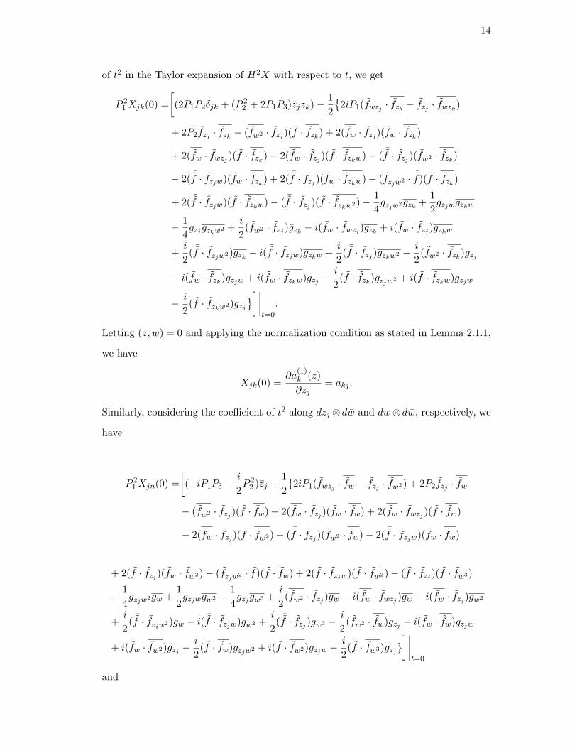
14
of t2 in the Taylor expansion of H2X with respect to t, we get
P 21Xjk(0) =
[(2P1P2δjk + (P 2
2 + 2P1P3)zjzk)−12
2iP1(fwzj · fzk − fzj · fwzk)
+ 2P2fzj · fzk − (fw2 · fzj )(f · fzk) + 2(fw · fzj )(fw · fzk)
+ 2(fw · fwzj )(f · fzk)− 2(fw · fzj )(f · fzkw)− ( ¯f · fzj )(fw2 · fzk)
− 2( ¯f · fzjw)(fw · fzk) + 2( ¯
f · fzj )(fw · fzkw)− (fzjw2 · ¯f)(f · fzk)
+ 2( ¯f · fzjw)(f · fzkw)− ( ¯
f · fzj )(f · fzkw2)− 14gzjw2gzk +
12gzjwgzkw
− 14gzjgzkw2 +
i
2(fw2 · fzj )gzk − i(fw · fwzj )gzk + i(fw · fzj )gzkw
+i
2( ¯f · fzjw2)gzk − i(
¯f · fzjw)gzkw +
i
2( ¯f · fzj )gzkw2 −
i
2(fw2 · fzk)gzj
− i(fw · fzk)gzjw + i(fw · fzkw)gzj −i
2(f · fzk)gzjw2 + i(f · fzkw)gzjw
− i
2(f · fzkw2)gzj
]∣∣∣∣t=0
.
Letting (z, w) = 0 and applying the normalization condition as stated in Lemma 2.1.1,
we have
Xjk(0) =∂a
(1)k (z)∂zj
= akj .
Similarly, considering the coefficient of t2 along dzj ⊗ dw and dw⊗ dw, respectively, we
have
P 21Xjn(0) =
[(−iP1P3 −
i
2P 2
2 )zj −122iP1(fwzj · fw − fzj · fw2) + 2P2fzj · fw
− (fw2 · fzj )(f · fw) + 2(fw · fzj )(fw · fw) + 2(fw · fwzj )(f · fw)
− 2(fw · fzj )(f · fw2)− ( ¯f · fzj )(fw2 · fw)− 2( ¯
f · fzjw)(fw · fw)
+ 2( ¯f · fzj )(fw · fw2)− (fzjw2 · ¯
f)(f · fw) + 2( ¯f · fzjw)(f · fw2)− ( ¯
f · fzj )(f · fw3)
− 14gzjw2gw +
12gzjwgw2 −
14gzjgw3 +
i
2(fw2 · fzj )gw − i(fw · fwzj )gw + i(fw · fzj )gw2
+i
2( ¯f · fzjw2)gw − i( ¯
f · fzjw)gw2 +i
2( ¯f · fzj )gw3 −
i
2(fw2 · fw)gzj − i(fw · fw)gzjw
+ i(fw · fw2)gzj −i
2(f · fw)gzjw2 + i(f · fw2)gzjw −
i
2(f · fw3)gzj
]∣∣∣∣t=0
and
15
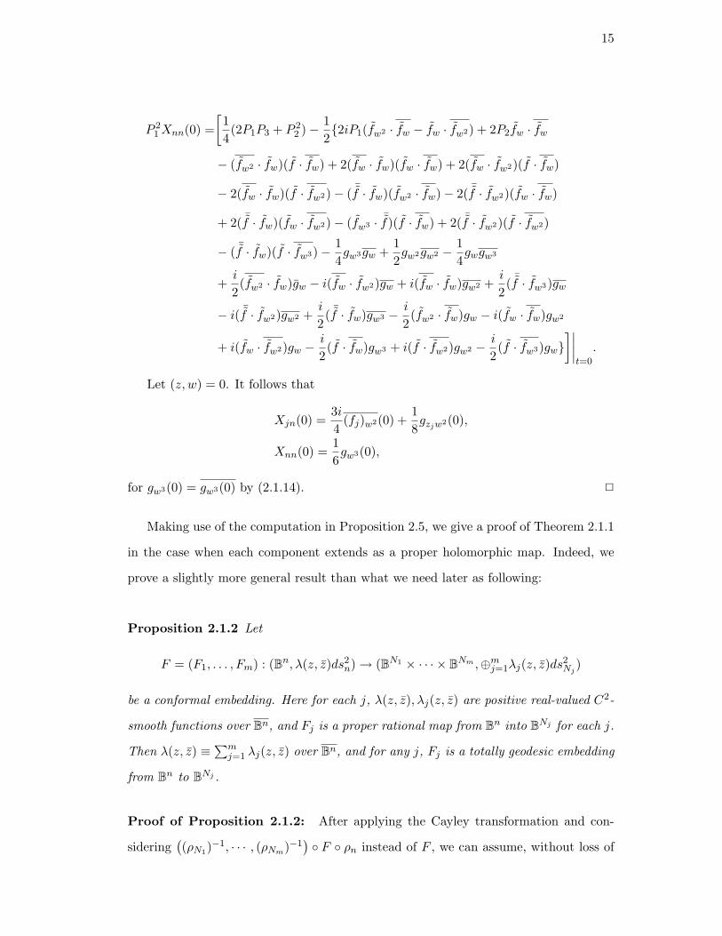
P 21Xnn(0) =
[14
(2P1P3 + P 22 )− 1
22iP1(fw2 · fw − fw · fw2) + 2P2fw · fw
− (fw2 · fw)(f · fw) + 2(fw · fw)(fw · fw) + 2(fw · fw2)(f · fw)
− 2(fw · fw)(f · fw2)− ( ¯f · fw)(fw2 · fw)− 2( ¯
f · fw2)(fw · fw)
+ 2( ¯f · fw)(fw · fw2)− (fw3 · ¯
f)(f · fw) + 2( ¯f · fw2)(f · fw2)
− ( ¯f · fw)(f · fw3)− 1
4gw3gw +
12gw2gw2 −
14gwgw3
+i
2(fw2 · fw)gw − i(fw · fw2)gw + i(fw · fw)gw2 +
i
2( ¯f · fw3)gw
− i( ¯f · fw2)gw2 +
i
2( ¯f · fw)gw3 −
i
2(fw2 · fw)gw − i(fw · fw)gw2
+ i(fw · fw2)gw −i
2(f · fw)gw3 + i(f · fw2)gw2 −
i
2(f · fw3)gw
]∣∣∣∣t=0
.
Let (z, w) = 0. It follows that
Xjn(0) =3i4
(fj)w2(0) +18gzjw2(0),
Xnn(0) =16gw3(0),
for gw3(0) = gw3(0) by (2.1.14). 2
Making use of the computation in Proposition 2.5, we give a proof of Theorem 2.1.1
in the case when each component extends as a proper holomorphic map. Indeed, we
prove a slightly more general result than what we need later as following:
Proposition 2.1.2 Let
F = (F1, . . . , Fm) : (Bn, λ(z, z)ds2n)→ (BN1 × · · · × BNm ,⊕mj=1λj(z, z)ds
2Nj )
be a conformal embedding. Here for each j, λ(z, z), λj(z, z) are positive real-valued C2-
smooth functions over Bn, and Fj is a proper rational map from Bn into BNj for each j.
Then λ(z, z) ≡∑m
j=1 λj(z, z) over Bn, and for any j, Fj is a totally geodesic embedding
from Bn to BNj .
Proof of Proposition 2.1.2: After applying the Cayley transformation and con-
sidering((ρN1)−1, · · · , (ρNm)−1
) F ρn instead of F , we can assume, without loss of
16
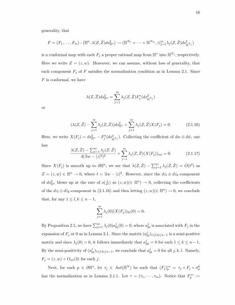
generality, that
F = (F1, . . . , Fm) : (Hn, λ(Z, Z)ds2Hn)→ (HN1 × · · · ×HNm ,⊕mj=1λj(Z, Z)ds2
HNj )
is a conformal map with each Fj a proper rational map from Hn into HNj , respectively.
Here we write Z = (z, w). Moreover, we can assume, without loss of generality, that
each component Fj of F satisfies the normalization condition as in Lemma 2.1. Since
F is conformal, we have
λ(Z, Z)ds2Hn =
m∑j=1
λj(Z, Z)F ∗j (ds2HNj )
or
(λ(Z, Z)−m∑j=1
λj(Z, Z))ds2Hn +
m∑j=1
λj(Z, Z)X(Fj) = 0. (2.1.16)
Here, we write X(Fj) = ds2Hn − F ∗j (ds2
HNj). Collecting the coefficient of dw ⊗ dw, one
hasλ(Z, Z)−
∑mj=1 λj(Z, Z)
4(=w − |z|2)2+
m∑j=1
λj(Z, Z)(X(Fj))nn = 0. (2.1.17)
Since X(Fj) is smooth up to ∂Hn, we see that λ(Z, Z) −∑m
j=1 λj(Z, Z) = O(t2) as
Z = (z, w) ∈ Hn → 0, where t = =w − |z|2. However, since the dzl ⊗ dzk-component
of ds2Hn blows up at the rate of o( 1
t2) as (z, w)(∈ Hn) → 0, collecting the coefficients
of the dzl ⊗ dzk-component in (2.1.16) and then letting (z, w)(∈ Hn)→ 0, we conclude
that, for any 1 ≤ l, k ≤ n− 1,
m∑j=1
λj(0)(X(Fj))kl(0) = 0.
By Proposition 2.5, we have∑m
j=1 λj(0)ajlk(0) = 0, where ajkl is associated with Fj in the
expansion of Fj at 0 as in Lemma 2.1. Since the matrix (ajkl)1≤l,k≤n−1 is a semi-positive
matrix and since λj(0) > 0, it follows immediately that ajkk = 0 for each 1 ≤ k ≤ n− 1.
By the semi-positivity of (ajkl)1≤l,k≤n−1, we conclude that ajlk = 0 for all j, k, l. Namely,
Fj = (z, w) +Owt(3) for each j.
Next, for each p ∈ ∂Hn, let τj ∈ Aut(HN ) be such that (Fj)∗∗p = τj Fj σ0p
has the normalization as in Lemma 2.1.1. Let τ = (τ1, · · · , τm). Notice that F ∗∗p :=
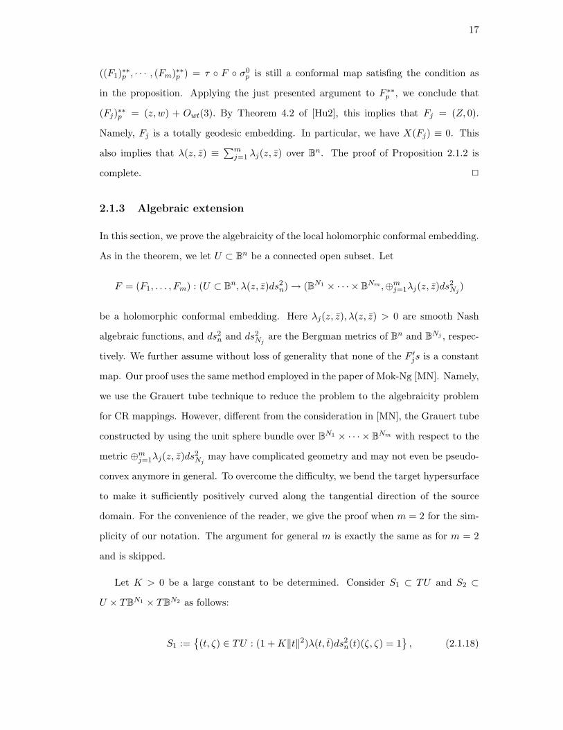
17
((F1)∗∗p , · · · , (Fm)∗∗p ) = τ F σ0p is still a conformal map satisfing the condition as
in the proposition. Applying the just presented argument to F ∗∗p , we conclude that
(Fj)∗∗p = (z, w) + Owt(3). By Theorem 4.2 of [Hu2], this implies that Fj = (Z, 0).
Namely, Fj is a totally geodesic embedding. In particular, we have X(Fj) ≡ 0. This
also implies that λ(z, z) ≡∑m
j=1 λj(z, z) over Bn. The proof of Proposition 2.1.2 is
complete. 2
2.1.3 Algebraic extension
In this section, we prove the algebraicity of the local holomorphic conformal embedding.
As in the theorem, we let U ⊂ Bn be a connected open subset. Let
F = (F1, . . . , Fm) : (U ⊂ Bn, λ(z, z)ds2n)→ (BN1 × · · · × BNm ,⊕mj=1λj(z, z)ds
2Nj )
be a holomorphic conformal embedding. Here λj(z, z), λ(z, z) > 0 are smooth Nash
algebraic functions, and ds2n and ds2
Njare the Bergman metrics of Bn and BNj , respec-
tively. We further assume without loss of generality that none of the F ′js is a constant
map. Our proof uses the same method employed in the paper of Mok-Ng [MN]. Namely,
we use the Grauert tube technique to reduce the problem to the algebraicity problem
for CR mappings. However, different from the consideration in [MN], the Grauert tube
constructed by using the unit sphere bundle over BN1 × · · · × BNm with respect to the
metric ⊕mj=1λj(z, z)ds2Nj
may have complicated geometry and may not even be pseudo-
convex anymore in general. To overcome the difficulty, we bend the target hypersurface
to make it sufficiently positively curved along the tangential direction of the source
domain. For the convenience of the reader, we give the proof when m = 2 for the sim-
plicity of our notation. The argument for general m is exactly the same as for m = 2
and is skipped.
Let K > 0 be a large constant to be determined. Consider S1 ⊂ TU and S2 ⊂
U × TBN1 × TBN2 as follows:
S1 :=
(t, ζ) ∈ TU : (1 +K‖t‖2)λ(t, t)ds2n(t)(ζ, ζ) = 1
, (2.1.18)

18
S2 := (t, z, ξ, w, η) ∈ U × TBN1 × TBN2 :
(1 +K‖t‖2)[λ1(t, t)ds2N1
(z)(ξ, ξ) + λ2(t, t)ds2N2
(w)(η, η)] = 1.(2.1.19)
The defining functions ρ1, ρ2 of S1, S2 are, respectively, as follows:
ρ1 = (1 +K‖t‖2)λ(t, t)ds2n(t)(ζ, ζ)− 1,
ρ2 = (1 +K‖t‖2)[λ1(t, t)ds2N1
(z)(ξ, ξ) + λ2(t, t)ds2N2
(w)(η, η)]− 1.
Then one can easily check that the map (id, F1, dF1, F2, dF2) maps S1 to S2 according
to the metric equation
λ(t, t)ds2n = λ1(t, t)F ∗1 (ds2
N1) + λ2(t, t)F ∗2 (ds2
N2).
Lemma 2.1.4 S1, S2 are both real algebraic hypersurfaces. Moreover for K sufficiently
large, S1 is smoothly strongly pseudoconvex. For any ξ 6= 0, η 6= 0, (0, 0, ξ, 0, η) ∈ S2 is
a smooth strongly pseudoconvex point when K is sufficiently large, where K depends on
the choice of ξ and η.
Proof It follows immediately from defining functions that S1, S2 are smooth real al-
gebraic hypersurfaces. We show the strong pseudoconvexity of S2 at (0, 0, ξ, 0, η) as
follows: (The strong pseudoconvexity of S1 follows from the same computation.)
By applying ∂∂ to ρ2 at (0, 0, ξ, 0, η), we have the following Hessian matrix
A 0 D1 0 D2
0 B1 0 0 0
D1 0 C1 0 0
0 0 0 B2 0
D2 0 0 0 C2
(2.1.20)
where
(A1)titj (0, 0, ξ, 0, η) = ∂ti∂tjρ2(0, 0, ξ, 0, η)
= K(λ1(0)|ξ|2 + λ2(0)|η|2)δij + ∂ti∂tjλ1(0)|ξ|2 + ∂ti∂tjλ2(0)|η|2
≥ δK(|ξ|2 + |η|2)δij ,
(2.1.21)
19
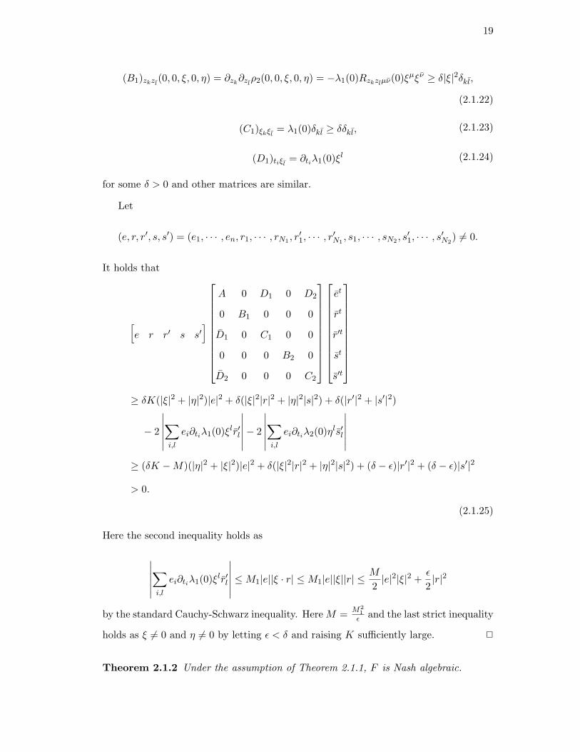
(B1)zkzl(0, 0, ξ, 0, η) = ∂zk∂zlρ2(0, 0, ξ, 0, η) = −λ1(0)Rzkzlµν(0)ξµξν ≥ δ|ξ|2δkl,
(2.1.22)
(C1)ξkξl = λ1(0)δkl ≥ δδkl, (2.1.23)
(D1)tiξl = ∂tiλ1(0)ξl (2.1.24)
for some δ > 0 and other matrices are similar.
Let
(e, r, r′, s, s′) = (e1, · · · , en, r1, · · · , rN1 , r′1, · · · , r′N1
, s1, · · · , sN2 , s′1, · · · , s′N2
) 6= 0.
It holds that
[e r r′ s s′
]
A 0 D1 0 D2
0 B1 0 0 0
D1 0 C1 0 0
0 0 0 B2 0
D2 0 0 0 C2
et
rt
r′t
st
s′t
≥ δK(|ξ|2 + |η|2)|e|2 + δ(|ξ|2|r|2 + |η|2|s|2) + δ(|r′|2 + |s′|2)
− 2
∣∣∣∣∣∣∑i,l
ei∂tiλ1(0)ξlr′l
∣∣∣∣∣∣− 2
∣∣∣∣∣∣∑i,l
ei∂tiλ2(0)ηls′l
∣∣∣∣∣∣≥ (δK −M)(|η|2 + |ξ|2)|e|2 + δ(|ξ|2|r|2 + |η|2|s|2) + (δ − ε)|r′|2 + (δ − ε)|s′|2
> 0.
(2.1.25)
Here the second inequality holds as
∣∣∣∣∣∣∑i,l
ei∂tiλ1(0)ξlr′l
∣∣∣∣∣∣ ≤M1|e||ξ · r| ≤M1|e||ξ||r| ≤M
2|e|2|ξ|2 +
ε
2|r|2
by the standard Cauchy-Schwarz inequality. Here M = M21ε and the last strict inequality
holds as ξ 6= 0 and η 6= 0 by letting ε < δ and raising K sufficiently large. 2
Theorem 2.1.2 Under the assumption of Theorem 2.1.1, F is Nash algebraic.
20
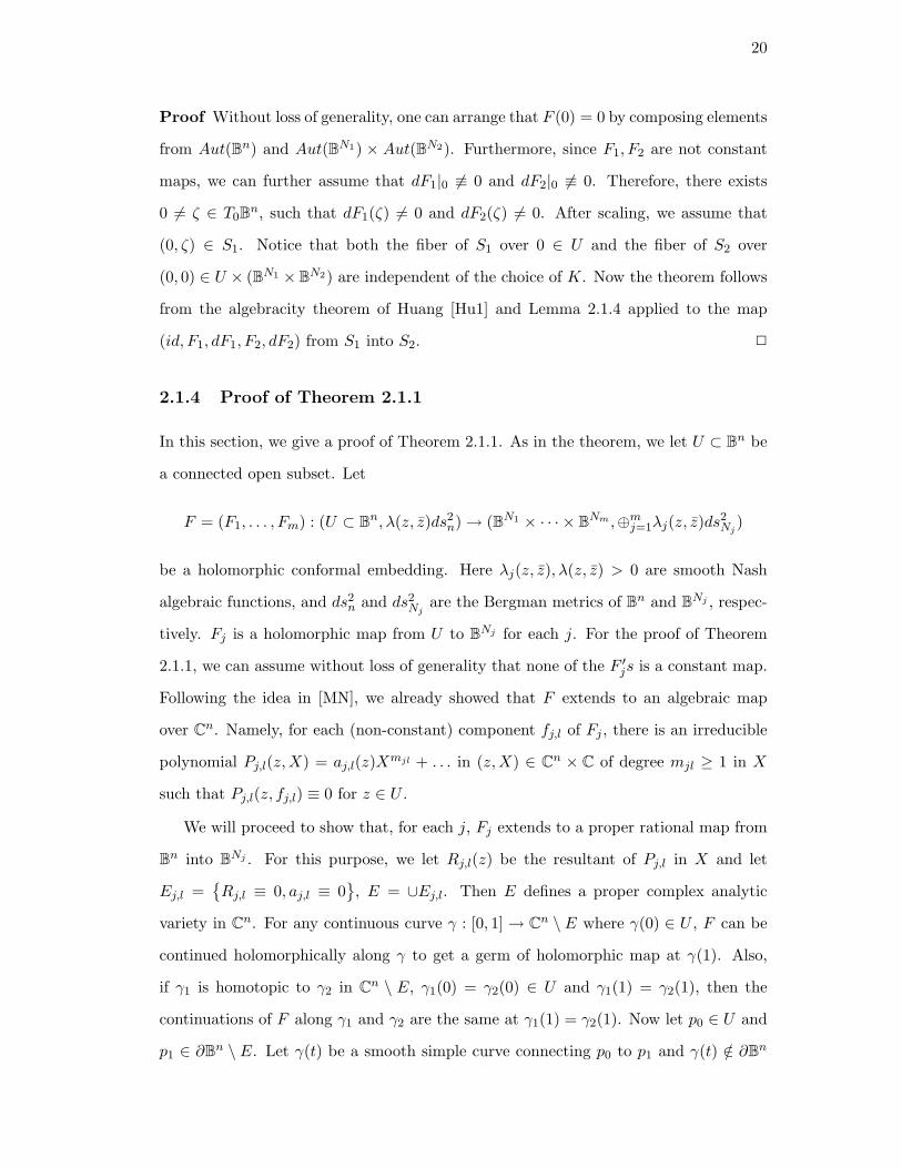
Proof Without loss of generality, one can arrange that F (0) = 0 by composing elements
from Aut(Bn) and Aut(BN1) × Aut(BN2). Furthermore, since F1, F2 are not constant
maps, we can further assume that dF1|0 6≡ 0 and dF2|0 6≡ 0. Therefore, there exists
0 6= ζ ∈ T0Bn, such that dF1(ζ) 6= 0 and dF2(ζ) 6= 0. After scaling, we assume that
(0, ζ) ∈ S1. Notice that both the fiber of S1 over 0 ∈ U and the fiber of S2 over
(0, 0) ∈ U × (BN1 ×BN2) are independent of the choice of K. Now the theorem follows
from the algebracity theorem of Huang [Hu1] and Lemma 2.1.4 applied to the map
(id, F1, dF1, F2, dF2) from S1 into S2. 2
2.1.4 Proof of Theorem 2.1.1
In this section, we give a proof of Theorem 2.1.1. As in the theorem, we let U ⊂ Bn be
a connected open subset. Let
F = (F1, . . . , Fm) : (U ⊂ Bn, λ(z, z)ds2n)→ (BN1 × · · · × BNm ,⊕mj=1λj(z, z)ds
2Nj )
be a holomorphic conformal embedding. Here λj(z, z), λ(z, z) > 0 are smooth Nash
algebraic functions, and ds2n and ds2
Njare the Bergman metrics of Bn and BNj , respec-
tively. Fj is a holomorphic map from U to BNj for each j. For the proof of Theorem
2.1.1, we can assume without loss of generality that none of the F ′js is a constant map.
Following the idea in [MN], we already showed that F extends to an algebraic map
over Cn. Namely, for each (non-constant) component fj,l of Fj , there is an irreducible
polynomial Pj,l(z,X) = aj,l(z)Xmjl + . . . in (z,X) ∈ Cn × C of degree mjl ≥ 1 in X
such that Pj,l(z, fj,l) ≡ 0 for z ∈ U .
We will proceed to show that, for each j, Fj extends to a proper rational map from
Bn into BNj . For this purpose, we let Rj,l(z) be the resultant of Pj,l in X and let
Ej,l =Rj,l ≡ 0, aj,l ≡ 0
, E = ∪Ej,l. Then E defines a proper complex analytic
variety in Cn. For any continuous curve γ : [0, 1] → Cn \ E where γ(0) ∈ U , F can be
continued holomorphically along γ to get a germ of holomorphic map at γ(1). Also,
if γ1 is homotopic to γ2 in Cn \ E, γ1(0) = γ2(0) ∈ U and γ1(1) = γ2(1), then the
continuations of F along γ1 and γ2 are the same at γ1(1) = γ2(1). Now let p0 ∈ U and
p1 ∈ ∂Bn \ E. Let γ(t) be a smooth simple curve connecting p0 to p1 and γ(t) /∈ ∂Bn
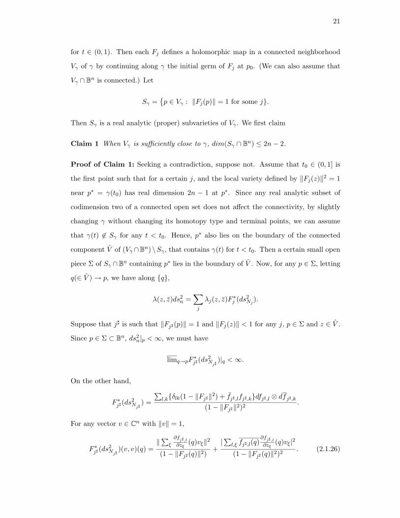
21
for t ∈ (0, 1). Then each Fj defines a holomorphic map in a connected neighborhood
Vγ of γ by continuing along γ the initial germ of Fj at p0. (We can also assume that
Vγ ∩ Bn is connected.) Let
Sγ =p ∈ Vγ : ‖Fj(p)‖ = 1 for some j.
Then Sγ is a real analytic (proper) subvarieties of Vγ . We first claim
Claim 1 When Vγ is sufficiently close to γ, dim(Sγ ∩ Bn) ≤ 2n− 2.
Proof of Claim 1: Seeking a contradiction, suppose not. Assume that t0 ∈ (0, 1] is
the first point such that for a certain j, and the local variety defined by ‖Fj(z)‖2 = 1
near p∗ = γ(t0) has real dimension 2n − 1 at p∗. Since any real analytic subset of
codimension two of a connected open set does not affect the connectivity, by slightly
changing γ without changing its homotopy type and terminal points, we can assume
that γ(t) 6∈ Sγ for any t < t0. Hence, p∗ also lies on the boundary of the connected
component V of (Vγ ∩Bn)\Sγ , that contains γ(t) for t < t0. Then a certain small open
piece Σ of Sγ ∩Bn containing p∗ lies in the boundary of V . Now, for any p ∈ Σ, letting
q(∈ V )→ p, we have along q,
λ(z, z)ds2n =
∑j
λj(z, z)F ∗j (ds2Nj ).
Suppose that j] is such that ‖Fj](p)‖ = 1 and ‖Fj(z)‖ < 1 for any j, p ∈ Σ and z ∈ V .
Since p ∈ Σ ⊂ Bn, ds2n|p <∞, we must have
limq→pF∗j](ds
2Nj]
)|q <∞.
On the other hand,
F ∗j](ds2Nj]
) =
∑l,kδlk(1− ‖Fj]‖2) + fj],lfj],kdfj],l ⊗ df j],k
(1− ‖Fj]‖2)2.
For any vector v ∈ Cn with ‖v‖ = 1,
F ∗j](ds2Nj]
)(v, v)(q) =‖∑
ξ
∂fj],l
∂zξ(q)vξ‖2
(1− ‖Fj](q)‖2)+|∑
l,ξ fj],l(q)∂fj],l
∂zξ(q)vξ|2
(1− ‖Fj](q)‖2)2. (2.1.26)
22
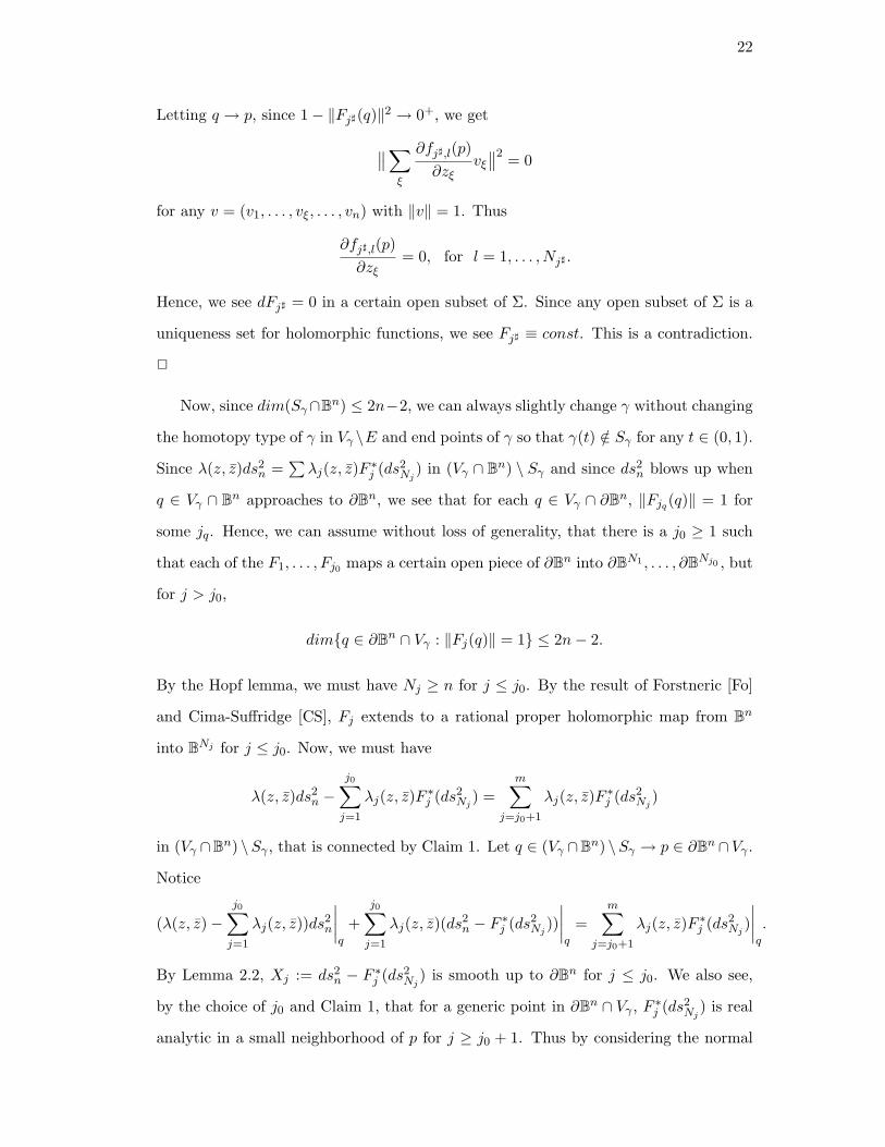
Letting q → p, since 1− ‖Fj](q)‖2 → 0+, we get
∥∥∑ξ
∂fj],l(p)∂zξ
vξ∥∥2 = 0
for any v = (v1, . . . , vξ, . . . , vn) with ‖v‖ = 1. Thus
∂fj],l(p)∂zξ
= 0, for l = 1, . . . , Nj] .
Hence, we see dFj] = 0 in a certain open subset of Σ. Since any open subset of Σ is a
uniqueness set for holomorphic functions, we see Fj] ≡ const. This is a contradiction.
2
Now, since dim(Sγ∩Bn) ≤ 2n−2, we can always slightly change γ without changing
the homotopy type of γ in Vγ \E and end points of γ so that γ(t) /∈ Sγ for any t ∈ (0, 1).
Since λ(z, z)ds2n =
∑λj(z, z)F ∗j (ds2
Nj) in (Vγ ∩ Bn) \ Sγ and since ds2
n blows up when
q ∈ Vγ ∩ Bn approaches to ∂Bn, we see that for each q ∈ Vγ ∩ ∂Bn, ‖Fjq(q)‖ = 1 for
some jq. Hence, we can assume without loss of generality, that there is a j0 ≥ 1 such
that each of the F1, . . . , Fj0 maps a certain open piece of ∂Bn into ∂BN1 , . . . , ∂BNj0 , but
for j > j0,
dimq ∈ ∂Bn ∩ Vγ : ‖Fj(q)‖ = 1 ≤ 2n− 2.
By the Hopf lemma, we must have Nj ≥ n for j ≤ j0. By the result of Forstneric [Fo]
and Cima-Suffridge [CS], Fj extends to a rational proper holomorphic map from Bn
into BNj for j ≤ j0. Now, we must have
λ(z, z)ds2n −
j0∑j=1
λj(z, z)F ∗j (ds2Nj ) =
m∑j=j0+1
λj(z, z)F ∗j (ds2Nj )
in (Vγ ∩Bn) \Sγ , that is connected by Claim 1. Let q ∈ (Vγ ∩Bn) \Sγ → p ∈ ∂Bn ∩Vγ .
Notice
(λ(z, z)−j0∑j=1
λj(z, z))ds2n
∣∣∣∣q
+j0∑j=1
λj(z, z)(ds2n − F ∗j (ds2
Nj ))∣∣∣∣q
=m∑
j=j0+1
λj(z, z)F ∗j (ds2Nj )∣∣∣∣q
.
By Lemma 2.2, Xj := ds2n − F ∗j (ds2
Nj) is smooth up to ∂Bn for j ≤ j0. We also see,
by the choice of j0 and Claim 1, that for a generic point in ∂Bn ∩ Vγ , F ∗j (ds2Nj
) is real
analytic in a small neighborhood of p for j ≥ j0 + 1. Thus by considering the normal
23
component as before in the above equation, we see that λ(z, z) −∑j0
j=1 λj(z, z) has
double vanishing order in an open set of the unit sphere. Since λ(z, z)−∑j0
j=1 λj(z, z)
is real analytic over Cn, we obtain
λ(z, z)−j0∑j=1
λj(z, z) = (1− |z|2)2ψ(z, z). (2.1.27)
Here ψ is a certain real analytic function over Cn. Next, write
Y = (λ(z, z)−j0∑j=1
λj(z, z))ds2n.
Then Y extends real analytically to Cn. Write X =∑j0
1 λj(z, z)Xj . From what we
argued above, we easily see that there is a certain small neighborhood O of q ∈ ∂Bn in
Cn such that (1): we can holomorphically continue the initial germ of F in U through
a certain simple curve γ with γ(t) ∈ Bn for t ∈ (0, 1) to get a holomorpic map, still
denoted by F , over O; (2): ‖Fj‖ < 1 for j > j0 and ‖Fj(z)‖ > 1 for j ≤ j0 over O \ Bn;
and (3):
X =j0∑j=1
λj(z, z)(ds2n − F ∗j (ds2
Nj )) =j0∑j=1
λj(z, z)Xj =m∑
j=j0+1
λj(z, z)F ∗j (ds2Nj )− Y.
(2.1.28)
We mention that we are able to make |Fj | < 1 for any z ∈ O and j > j0 in the above
due to the fact that Vγ ∩ Bn \ Sγ , as defined before, is connected.
Now, let P be the union of the poles of F1, . . . , Fj0 . Fix a certain p∗ ∈ O∩ ∂Bn and
let E = E ∪ P. Then for any γ : [0, 1] → (Cn \ Bn) \ E with γ(0) = p∗, Fj extends
holomorphically to a small neighborhood Uγ of γ that contracts to γ. Still denote the
holomorphic continuation of Fj (from the initial germ of Fj at p∗ ∈ O) over Uγ by Fj .
If for some t ∈ (0, 1), ‖Fj(γ(t))‖ = 1, then we similarly have
Claim 2 Shrinking Uγ if necessary, we then have
dimp ∈ Uγ : ‖Fj(p)‖ = 1 for some j
≤ 2n− 2.
Proof of the Claim 2: Still seek for a contradiction, if we suppose not. Define Sγ in
a similar way. Without loss of generality, we assume that t0 ∈ (0, 1) is the first point
24
such that for a certain jt0 , the local variety defined by ‖Fjt0 (z)‖2 = 1 near γ(t0) has
real dimension 2n− 1 at γ(t0). Then, as before, we have
X =j0∑j=1
λj(z, z)(ds2n − F ∗j (ds2
Nj )) =m∑
j=j0+1
λj(z, z)F ∗j (ds2Nj )− Y (2.1.29)
in a connected component W of Uγ \Sγ that contains γ(t) for t << 1 with γ(t0) ∈ ∂W .
Now, for any qj(∈ W ) → p ∈ ∂W near p0 = γ(t0) and v ∈ Cn with ‖v‖ = 1, we have
the following:
j0∑j=1
λj(z, z)(‖∑ξ
∂fj,l∂zξ
(q)vξ‖2
(1− ‖Fj(q)‖2)+|∑
l,ξ fj,l(q)∂fj,l∂zξ
(q)vξ|2
(1− ‖Fj(q)‖2)2
)
=m∑
j=j0+1
λj(z, z)(‖∑ξ
∂fj,l∂zξ
(q)vξ‖2
(1− ‖Fj(q)‖2)+|∑
l,ξ fj,l(q)∂fj,l∂zξ
(q)vξ|2
(1− ‖Fj(q)‖2)2
)− Y (v, v).
(2.1.30)
Now, if p0 is not a point of codimension one for any local variety defined by ‖Fj(z)‖2 = 1
near p0 for j ≤ j0, then it has to be a codimension one point for a certain local variety
Sj′ defined by ‖Fj′(z)‖2 = 1 near p0 for j′ > j0. Let J be the collection of all such
j′. Let S0 be a small open piece of the boundary of W near p0. Then for a generic
p ∈ S0, the left hand side of (2.1.30) remains bounded as q → p ∈ S0. For a term
in the right hand side with index j ∈ J , if S0 ∩ Sj contains an open neigborhood of
∂W near p0, then it approaches to +∞ for a generic p unless Fj = constant as argued
before. The other terms on the right hand side remain bounded as q → p for a generic
p. This is a contradiction to the assumption that none of the Fj for j > j0 is constant.
Hence, we can assume that p0 is a point of codimension one for a local variety defined by
‖Fj(z)‖2 = 1 near p0 for a certain j ≤ j0. Let J be the set of indices such that for j′ ∈ J ,
we have j′ ≤ j0 and Sj′ := ‖Fj′‖ = 1 is a local real analytic variety of codimension
one near p0. For j > j0, since ‖Fj(z)‖ < 1 for z(∈ Uγ) ≈ p0 and since t0 is the first
point we have some j∗ with ‖Fj∗‖ = 1 defining a variety of real codimension one, we see
that ‖Fj(z)‖ < 1 for z(∈W ) ≈ p0. Define S0 similarly, as an open piece of ∂W . Hence,
as q(∈ W ) → p ∈ S0, the right hand side of (2.1.30) remains to be non-negative. On
the other hand, in the left hand side of (2.1.30) , for any j′ ∈ J with Sj′ ∩S0 containing
an open piece of ∂W near p0, if the numerator |∑
l,ξ fj′,l(q)∂fj′,l∂zξ
(q)vξ|2 of the last term
does not go to 0 for some vectors v, then the term with index j′ on the left hand side
25
would go to −∞ for a generic p ∈ S0. If this happens to such j′, the left hand side
would approach to −∞. Notice that all other terms on the right hand side remain
bounded as q → p ∈ S0 for a generic p. This is impossible. Therefore we must have
for some j′ ∈ J that |∑
l fj′,l(q)∂fj′,l∂zξ
(q)|2 =∂
∑l |fj′,l|2∂zξ
(q) =∂‖Fj′‖2∂zξ
(q) → 0 and thus∂‖Fj′‖2∂zξ
(p) = 0 for all ξ and p ∈ Sj′ . This immediately gives the equality d(‖Fj′‖2) = 0
along Sj′ . Assume, without loss of generality, that p0 is also a smooth point of Sj′ .
If Sj′ has no complex hypersurface passing through p0, by a result of Trepreau [Tr],
the union of the image of local holomoprphic disks attached to Sj′ passing through p0
fills in an open subset. Since Fj′ is not constant, there is a small holomorphic disk
smooth up to the boundary φ(τ) : B1 → Cn such that φ(∂B1) ⊂ Sj′ , φ(1) = p0 and Fj′
is not constant along φ. Since ∂BNj′ does not contain any non-trival complex curves,
r = (‖Fj′‖2−1)φ 6≡ 0. Applying the maximum principle and then the Hopf lemma to
the subharmonic function r = (‖Fj′‖2−1)φ, we see that the outward normal derivative
of r at τ = 1 is positive. This contradicts the fact that d(‖Fj′‖2) = 0 along Sj′ . We
can argue the same way for points p ∈ Sj′ near p0 to conclude that for any p ∈ Sj′ near
p0, there is a complex hypersurface contained in Sj′ passing through p. Namely, Sj′ is
Levi flat, foliated by a family of smooth complex hypersurfaces denoted by Yη with real
parameter η near p0. Let Z be a holomorphic vector field along Yη. We then easily see
that 0 = ZZ(‖Fj′‖2 − 1) =∑Nj′
k=1 |Z(fj′,k)|2. Thus, we see that Fj′ is constant along
each Yη. Hence, Fj′ can not be a local embedding at each point of Sj′ . On the other
hand, noticing that Fj′ is a proper holomorphic map from Bn into BN ′ , Fj′ is a local
embedding near ∂Bn. Hence, the set of points where Fj′ is not a local embedding can
be at most of complex codimension one (and thus real codimension two). This is a
contradiction. This proves Claim 2.
Hence, we see that E = p ∈ (Cn\Bn)\E : some branch, obtained by the holomorphic
continuation through curves described before, of Fj for some j maps p to ∂BNj is a
real analytic variety of real dimension at most 2n− 2. Now, for any p ∈ (Cn \ Bn) \ E,
any curve γ : [0, 1] → (Cn \ Bn) \ E with γ(0) = p∗ ∈ O ∩ ∂Bn and γ(1) = p, we can
homotopically change γ in (Cn \ Bn) \ E (but without changing the terminal points)
such that γ(t) /∈ E for t ∈ (0, 1). Now, the holomorphic continuation of the initial germ
26
of Fj from p∗ never cuts ∂BNj along γ(t) (0 < t < 1). We thus see that ‖Fj(p)‖ ≤ 1 for
j > j0.
Let (fj,l)k;pnjlk=1 be all possible (distinct) germs of holomorphic functions that we
can get at p by the holomorphic continuation, along curves described above in (Cn\Bn)\
E, of fj,l. Let σjl,τ be the fundamental symmetric function of (fj,l)k;pnjlk=1 of degree
τ . Then σjl,τ well defines a holomorphic function over (Cn \Bn). ‖σjl,τ‖ is bounded in
(Cn \Bn)\ E. By the Riemann removable singularity theorem, σjl,τ is holomorphic over
(Cn \ Bn). By the Hartogs lemma, σjl,τ extends to a bounded holomorphic function
over Cn. Hence, by the Liouville theorem, σjl,τ ≡ const. This forces (fj,l)k and thus
Fj for j > j0 to be constant. We obtain a contradiction. This proves that each Fj
extends to a proper rational map from Bn into BNj . Together with Proposition 2.1.2,
we complete the proof of the main Theorem. 2
We conclude the section with a remark: The regularity of λj , λ can be reduced to
be only real analytic in the complement of a certain real codimension two subset. This
is obvious from our proof for Theorem 2.1.1.
2.2 Rigidity for local holomorphic isometric embeddings from the pro-
jective space into the product of projective spaces
In this section, we try to attack the classification problem 1.1.1. Let
[z0, · · · , zn]
be
the homogeneous coordinate of Pn and ωn be the Fubini-Study metric. Let U0 := z0 6=
0 be one coordinate chart of Pn, and the coordinate is given by xi = ziz0
. Then on U0,
the Fubini-Study metric can be written as:
ωn =√−1∂∂ log
(1 +
n∑i=1
|xi|2).
Calabi proved the local rigidity and global extension theorem for the local holomor-
phic embedding from a Kahler manifold into the projective space equipped with the
Fubini-Study metric. We are going to apply them in the proof of our theorems.
27
Theorem 2.2.1 [Ca] If M is a Kahler manifold and assume that an open set G ⊂
M admits a holomorphic isometric embedding into (PN , ωN ), then the embedding is
uniquely determined modular the group of isometries Isom(PN , ωN ).
Theorem 2.2.2 [Ca] Let M is a simply connected Kahler manifold and let f : G ⊂
M → PN be an holomorphic isometric embedding with respect to the Fubini-Study metric
ωN . Then there exists a global mapping F : M → PN extending f .
Definition 2.2.1 Let f, g : M → Pn are holomorphic maps. f, g are called equivalent
if f, g are equivalent up to the group of isometries of Pn. More precisely, there exists
σ ∈ Isom(Pn, ωn), such that f = σ g.
From now on, we consider our classification question 1.1.1. Let λl > 0 be a positive
constant and let
F = (F1, · · · , Fp) : (U ⊂ Pn, ωn)→ (PN1 × · · · × PNp ,⊕pl=1λlωNl)
be a local holomorphic isometric imbedding with respect to Fubini-Study metrics, i.e.
ωn =∑l
λlF∗l ωNl .
First, we prove the global extension theorem in a special case.
Theorem 2.2.3 Under the above assumption and further assuming λl ∈ Q+, F extends
F to Pn as a holomorphic isometry, i.e. there exists a holomorphic map
F = (F1, · · · , Fp) : Pn → PN1 × · · · × PNp
such that
F∣∣U
= F and ωn =∑l
λlF∗l ωNl .
Proof For simplicity, we give the proof for p = 2. By multiplying the common denom-
inators of λl, still denoted by λl, we assume that
F = (F1, F2) : U ⊂ Pn → PN1 × PN2
with
28
λωn = λ1F∗1ωN1 + λ2F
∗2ωN2
where λ, λi are positive integers. Then one has the following diagram:
U ⊂ PnF- PN1 × PN2
PN
s
?
∩
G
-
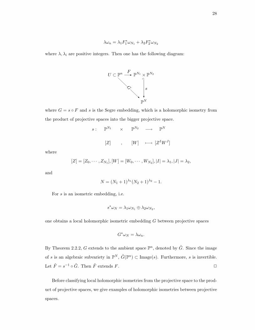
where G = s F and s is the Segre embedding, which is a holomorphic isometry from
the product of projective spaces into the bigger projective space.
s : PN1 × PN2 −→ PN
[Z] , [W ] 7−→ [ZIW J ]
where
[Z] = [Z0, · · · , ZN1 ], [W ] = [W0, · · · ,WN2 ], |I| = λ1, |J | = λ2,
and
N = (N1 + 1)λ1(N2 + 1)λ2 − 1.
For s is an isometric embedding, i.e.
s∗ωN = λ1ωN1 ⊕ λ2ωN2 ,
one obtains a local holomorphic isometric embedding G between projective spaces
G∗ωN = λωn.
By Theorem 2.2.2, G extends to the ambient space Pn, denoted by G. Since the image
of s is an algebraic subvariety in PN , G(Pn) ⊂ Image(s). Furthermore, s is invertible.
Let F = s−1 G. Then F extends F . 2
Before classifying local holomorphic isometries from the projective space to the prod-
uct of projective spaces, we give examples of holomorphic isometries between projective
spaces.
29
Example 2.2.1 We start with the Veronese embedding with isometric constant 2.
vn,2 : Pn - P(n+1)(n+2)
2−1
[z] ⊂ - [√
2 cos(π
4δij)zizj ]
One can check thatn∑
i,j=0
|√
2 cos(π
4δij)zizj |2 =
( n∑i=0
|zi|2)2,
yielding
v∗n,2
(ω (n+1)(n+2)
2
)= 2ωn
by taking√−1∂∂ log. Let
Mn,2 =(n+ 1)(n+ 2)
2− 1.
One can check that Mn,2 is the smallest dimension of the projective space admitting
holomorphic isometry from Pn with isometric constant 2. Suppose that we have another
holomorphic embedding f : Pn → PN with
f∗ωN = 2ωn and N ≥Mn,2.
Then f is equivalent to (vn,2, 0, · · · , 0) by Theorem 2.2.1.
Similarly, one can also cook up the Veronese embedding vn,κ with any integer iso-
metric constant κ. Define Mn,κ to be the smallest dimension of the projective space
admitting holomorphic isometry from Pn with isometric constant κ and we have the
same rigidity property as above.
The following theorem gives the classification of the local holomorphic isometric
embedding when λl ∈ Q.
Theorem 2.2.4 We suppose the assumption in Theorem 2.2.3. Let κ1, · · · , κp ∈
(Z+)p satisfy
(i) Nl ≥Mn,κl for 1 ≤ l ≤ q,
(ii)∑p
l=1 κlλl = 1.
30
Then the possibility of κ1, · · · , κp gives the classification of F = (F1, · · · , Fp). In
particular, Fl is equivalent to the Veronese embedding Vn,κl with isometric constant κl
and Fl is a constant map if κl = 0.
Proof Recall that z = [z0, · · · , zn], w = [w0, · · · , wNl ] are the homogenous coordinates
for Pn and PNl respectively. We use the coordinates xi = ziz0
on U0 ⊂ Pn and let
V0,l = w0 6= 0 be a coordinate chart on PNl .
By Theorem 2.2.3, we know that Fl = (fl,0, · · · , fl,Nl) are all homogenous polyno-
mials of z mapping Pn into PNl . By composing with Isom(PNl , ωNl), we can assume
that Fl([1, 0, · · · , 0]) = [1, 0, · · · , 0]. Hence Fl maps some open subset of U0 into V0,l.
Let
rl,ql(x) =fl,ql(z)fl,0(z)
be a rational function in x for 1 ≤ ql ≤ Nl and write Fl = (rl,1(x), · · · , rl,Nl(x)). As Fl
is an isometric embedding, we have
√−1∂∂ log(1 +
n∑i=1
|xi|2) =∑l
λl√−1∂∂ log(1 +
Nl∑ql=1
|rl,ql(x)|2).
Getting rid of√−1∂∂, one has:
log(1 +n∑i=1
|xi|2) =∑l
λl log(1 +Nl∑ql=1
|rl,ql(x)|2) + Reh(x)
for some holomorphic function h(x).
Comparing the Taylor expansion of two sides, when rl,ql(0) = 0, the other two
quantities do not have the pure holomorphic and anti-holomorphic terms like xα, xα
except for Reh, implying that h = 0. Therefore,
1 +n∑i=1
|xi|2 =∏l
(1 +Nl∑ql=1
|rl,ql(x)|2)λl .
Note that the right hand side approaches∞ when x approaches any pole of rl,ql(x),
while the left hand is bounded, implying that rl,ql(x) is actually a polynomial. By
polarization (replacing xi by yi), it follows that:
31
1 +n∑i=1
xiyi =∏l
(1 +Nl∑ql=1
rl,ql(x)rl,ql(y))λl .
Since 1+∑n
i=1 xiyi is irreducible, and C[x, y] is a unique factorization domain, it follows
that
1 +Nl∑ql=1
rl,ql(x)rl,ql(y) = (1 +n∑i=1
xiyi)κl
for the possible integer κl satisfying condition (i) and (ii). This implies
1 +Nl∑ql=1
|rl,ql(x)|2 = (1 +n∑i=1
|xi|2)κl ,
meaning that Fl is an isometry from Pn to PNl with isometric constant κl. By Theorem
2.2.1, Fl is equivalent to the Veronese embedding Vn,κl .
If κl = 0, i.e.
1 +Nl∑ql=1
|rl,ql(x)|2 = 1,
it follows that rl,ql(x) ≡ 0, implying that Fl is a constant map. 2
32
Chapter 3
On the modified Kahler-Ricci flow
3.1 Preliminaries
Let X be a closed Kahler manifold of complex dimension n with a Kahler metric ω0,
and let ω∞ be a real, smooth, closed (1, 1)-form with [ω∞]n = 1. Let Ω be a smooth
volume form on X such that∫X Ω = 1. Set χ = ω0 − ω∞, ωt = ω∞ + e−tχ. Let
ϕ : [0,∞)×X → R be a smooth function such that ωt = ωt +√−1∂∂ϕ > 0. Consider
the following Monge-Ampere flow:
∂∂tϕ = log (ωt+
√−1∂∂ϕ)n
Ω ,
ϕ(0, ·) = 0.
(3.1.1)
Then the evolution for the corresponding Kahler metric is given by:
∂∂t ωt = −Ric(ωt) +Ric(Ω)− e−tχ,
ωt(0, ·) = ω0.
(3.1.2)
We will give some definitions before stating our theorem.
Definition 3.1.1 [γ] ∈ H1,1(X,C) is semi-positive if there exists γ′ ∈ [γ] such that
γ′ ≥ 0, and is big if [γ]n :=∫X γ
n > 0.
Definition 3.1.2 A closed, positive (1, 1)-current ω is called a singular Calabi-Yau
metric on X if ω is a smooth Kahler metric away from an analytic subvariety E ⊂ X
and satisfies Ric(ω) = 0 away from E.
33
Definition 3.1.3 A volume form Ω is called a Calabi-Yau volume form if
Ric(Ω) := −√−1∂∂ log Ω = 0.
Theorem 3.1.1 Let X be a Kahler manifold with a Kahler metric ω0. Suppose that
[ω∞] ∈ H1,1(X,C)∩H2(X,Z) is semi-positive and big. Then along the modified Kahler-
Ricci flow (3.1.2), ωt converges weakly in the sense of currents and converges locally
in C∞-norm away from a proper analytic subvariety of X to the unique solution of the
degenerate Monge-Ampere equation (ω∞ +√−1∂∂ψ)n = Ω.
Corollary 3.1.1 When X is a Calabi-Yau manifold and Ω is a Calabi-Yau volume
form, ωt converges to a singular Calabi-Yau metric.
As [ω∞] ∈ H1,1(X,C) ∩ H2(X,Z), there exists a line bundle L over X such that
ω∞ ∈ c1(L). Moreover, L is big when [ω∞] is semi-positive and big [De]. Hence X
is Moishezon. Furthermore, X is algebraic, for it is Kahler. Therefore, by applying
Kodaira lemma, we see that for any small positive number ε ∈ Q, there exists an
effective divisor E on X, such that [L]− ε[E] > 0. Therefore, there exists a hermitian
metric hE on E such that ω∞ − εRic(hE), denoted by ωE , is strictly positive for any ε
small. Let S be the defining section of the effective divisor E.
We now define some notations for the convenience of our later discussions. Let ∇, ∆
and ∂∂t − ∆ be the gradient operator, the Laplacian and the heat operator with respect
to the metric ωt respectively. Let Vt = [ωt]n with Vt uniformly bounded and V0 = 1.
Write ϕ = ∂ϕ∂t for simplicity.
Before proving the theorem, we would like to sketch the standard uniform estimates
of ϕ and recall some crucial estimates due to Zhang.
First of all, by the standard computation as in [Z3], the uniform upper bound of
∂∂tϕ is deduced from the maximum principle. Secondly, by the result of [Z2] [EGZ],
generalizing the theorem of Ko lodziej [K1] to the degenerate case, we have the C0-
estimate ‖u‖C0(X) ≤ C independent of t where u = ϕ −∫X ϕΩ. Then to estimate
∂∂tϕ locally, we will calculate ( ∂∂t − ∆)[ϕ+A(u− ε log ‖S‖2hE )], and then the maximum
principle yields ∂∂tϕ ≥ −C + α log ‖S‖2hE for C,α > 0.
34
Next, we follow the standard second order estimate as in [Y1] [Cao] [Si] [Ts]. Calcu-
lating ( ∂∂t − ∆)[log trωE+e−tχωt−A(u− ε log ‖S‖2hE )] and applying maximum principle,
we have: |∆ωEϕ| ≤ C. Then by using Schauder estimates and third order estimate as
in [Z3], we can obtain the local uniform estimate: For any k ≥ 0,K ⊂⊂ X \ E, there
exists Ck,K > 0, such that:
‖u‖Ck([0,+∞)×K) ≤ Ck,K . (3.1.3)
In [Z3], Zhang proved the following theorem by comparing (3.1.1) with the Kahler-
Ricci flow (3.1.4). We include the detail of the proof here for the sake of completeness.
This uniform lower bound appears to be crucial in the proof of the convergence.
Theorem 3.1.2 ([Z3]) There exists C > 0 such that ∂∂tϕ ≥ −C holds uniformly along
(3.1.1) or (3.1.2).
We derive a calculus lemma here for later application.
Lemma 3.1.1 Let f(t) ∈ C1([0,+∞)) be a non-negative function. If∫ +∞
0 f(t)dt <
+∞ and ∂f∂t is uniformly bounded, then f(t)→ 0 as t→ +∞.
Proof We prove this calculus lemma by contradiction. Suppose that there exist a
sequence ti → +∞ and δ > 0, such that f(ti) > δ. Since ∂f∂t is uniformly bounded,
there exist a sequence of connected, non-overlapping intervals Ii containing ti with fixed
length l, such that f(t) ≥ δ2 over Ii. Then
∫∪iIi f(t)dt ≥
∑i lδ2 → +∞, contradicting
with∫ +∞
0 f(t)dt < +∞. 2
Let ωt = ωt +√−1∂∂φ and ∆ be the Laplacian operator with respect to the metric
ωt. Consider the Monge-Ampere flow, as well as its corresponding evolution of metrics:
∂∂tφ = log (ωt+
√−1∂∂φ)n
Ω − φ,
φ(0, ·) = 0.
(3.1.4)
35
∂∂t ωt = −Ric(ωt) +Ric(Ω)− ωt + ω∞,
ωt(0, ·) = ω0.
(3.1.5)
The following theorem is proved in [Z1] and we sketch Zhang’s argument here.
Theorem 3.1.3 There exists C > 0, such that ∂∂tφ ≥ −C uniformly along (3.1.4).
Proof The standard computation shows:
(∂
∂t− ∆)(
∂φ
∂t+∂2φ
∂t2) ≤ −(
∂φ
∂t+∂2φ
∂t2).
Then the maximum principle yields:
∂
∂t(φ+
∂φ
∂t) ≤ C1e
−t,
which further implies:∂
∂tφ ≤ C2e
− t2 .
Hence φ + ∂φ∂t and φ are essentially decreasing along the flow, for example: ∂
∂t(φ +
φ + C1e−t) ≤ 0 and φ is uniformly bounded from above. As one also has the uni-
form estimate of φ that φ is uniformly bounded in Ck([0,∞) × K)-norm for any
k ≥ 0 and K ⊂⊂ X \ E, one can conclude that ∂φ∂t → 0 pointwisely away from E
by applying Lemma 3.1.1 to C2e− t
2 − ∂φ∂t . Suppose that φ∞ is the limit of φ. Then
φ∞ ∈ PSH(X,ω∞) and φ∞ is also the pointwise limit of φ+ ∂φ∂t away from E. By the
uniform estimate of φ once more, one knows that φ converges to φ∞ in C∞(K) for any
K ⊂⊂ X \ E. Then the convergence of (3.1.4) is obtained [TZha] in the sense that
eφ∞Ω = (ω∞ +√−1∂∂φ∞)n ← eφ+φΩ = (ωt +
√−1∂∂φ)n
in Ck(K)-norm for any k ≥ 0,K ⊂⊂ X \ E as t → +∞. Furthermore, by [K1],
φ(t, ·) ∈ L∞(X) for 0 ≤ t < ∞. In addition, (ω∞ +√−1∂∂φ∞)n does not charge any
pluri-polar set, in particular, the effective divisor E, as φ∞ is the decreasing limit of
φ(t, ·) + 2C2e− t
2 . Therefore,
36
eφ∞Ω = (ω∞ +√−1∂∂φ∞)n
holds in the sense of currents on X. On the other hand, from the pluri-potential theory
[Z2] [EGZ], we know that −C3 ≤ φ∞ − supX φ∞ ≤ C3 for C3 > 0 as ‖eφ∞‖Lp(Ω) < C4
for any p > 0 and supX φ∞ 6= −∞. By the essentially decreasing property, it follows
that away from E:
φ+ φ+ C1e−t ≥ φ∞ ≥ −C3 + sup
Xφ∞ ≥ −C5.
Hence the uniform lower bound of φ is obtained as φ is uniformly bounded from above
and φ is smooth on X.
2
We are now ready to give Zhang’s proof to Theorem 3.1.2.
Proof of Theorem 3.1.2:
Notice that ϕ, φ are solutions to equation (3.1.1) and (3.1.4) respectively. Fix T0 > 0.
Let κ(t, ·) = (1− e−T0)ϕ+ u− φ(t+ T0) with κ(0, ·) ≥ −C1. Then:
∂
∂tκ(t, ·) = ∆((1− e−T0)ϕ+ u) + u− φ(t+ T0)− n+ trωtωt+T0
= ∆((1− e−T0)ϕ+ u− φ(t+ T0)) + u− φ(t+ T0)− n+ trωtωt+T0
≥ ∆((1− e−T0)ϕ+ u− φ(t+ T0)) + ϕ− C2 + n(C3
eϕ)
1n ,
where the fact: u ≥ ϕ− C,−C ≤ ∂∂tφ ≤ C and ωt ≥ C3Ω are used.
Suppose that κ(t, ·) achieves minimum at (t0, p0) with t0 > 0. Then the maximum
principle yields ϕ(t0, p0) ≥ −C4. Hence ϕ is bounded from below. Suppose that κ(t, ·)
achieves minimum at t = 0. Then the theorem follows trivially. 2
37
3.2 Proof of Theorem 3.1.1
Inspired from the Mabuchi K-energy in the study on the convergence of the Kahler-
Ricci flow on Fano manifolds, we similarly define an energy functional as follows:
ν(ϕ) =∫X
log(ωt +
√−1∂∂ϕ)n
Ω(ωt +
√−1∂∂ϕ)n.
Next, we will give some properties of ν(ϕ) and then a key lemma for the proof of
the main theorem.
Proposition 3.2.1 ν(ϕ) is well-defined and there exists C > 0, such that −C < ν(ϕ) <
C along (3.1.2).
Proof It is easy to see that ν(ϕ) is well-defined. If we rewrite
ν(ϕ) =∫Xϕωnt ,
then ν(ϕ) is uniformly bounded from above and below by the uniform upper and lower
bound of ϕ. Here, we derive the uniform lower bound by Jensen’s inequality without
using Theorem 3.1.2:
ν(ϕ) = −Vt∫X
logΩωnt
ωntVt≥ −Vt log
∫X
ΩVt≥ −C,
as Vt is uniformly bounded. 2
Proposition 3.2.2 There exists constant C > 0 such that for all t > 0 along the flow
(3.1.2):∂
∂tν(ϕ) ≤ −
∫X‖∇ϕ‖2ωtω
nt + Ce−t. (3.2.1)
38
Proof Along the flow (3.1.2), we have:
∂
∂tν(ϕ) =
∫X
∆ϕωnt − e−t∫Xtrωtχω
nt − ne−t
∫Xϕχ ∧ ωn−1
t + n
∫Xϕ√−1∂∂ϕ ∧ ωn−1
t
= −∫X‖∇ϕ‖2ωtω
nt − ne−t
∫Xχ ∧ ωn−1
t − ne−t∫Xϕχ ∧ ωn−1
t
= −∫X‖∇ϕ‖2ωtω
nt − n[χ][ωt]n−1e−t − ne−t
∫Xϕ(ω0 − ω∞) ∧ ωn−1
t
≤ −∫X‖∇ϕ‖2ωtω
nt + n[χ][ωt]n−1e−t + Ce−t
∫X
(ω0 + ω∞) ∧ ωn−1t
= −∫X‖∇ϕ‖2ωtω
nt + [nχ+ Cω0 + Cω∞][ωt]n−1e−t
≤ −∫X‖∇ϕ‖2ωtω
nt + C ′e−t.
Notice that we used the evolution of ϕ and integration by parts in the first two equalities
and the uniform bound of ϕ in the first inequality and the last inequality holds since
ωt is uniformly bounded. 2
Lemma 3.2.1 On each K ⊂⊂ X \ E, ‖∇ω∞ϕ(t)‖2ω∞ → 0 uniformly as t→ +∞.
Proof Integrating (3.2.1) from 0 to T , we have:
−C ≤ ν(ϕ)(T )− ν(ϕ)(0) ≤ −∫ T
0
∫X‖∇ϕ‖2ωtω
nt dt+ C
for some constant C > 0. It follows that
∫ +∞
0
∫X‖∇ϕ‖2ωtω
nt dt ≤ 2C,
by letting T → +∞. Hence, (3.1.3) and Lemma 3.1.1 imply that for any compact set
K ′ ⊂ X \ E,
∫K′‖∇ϕ(t, ·)‖2ωtω
nt → 0. (3.2.2)
Now, assume that there exists δ > 0, zj ∈ K and tj →∞ such that ‖∇ω∞ϕ(tj , zj)‖2ω∞> δ. It follows from (3.1.3) that ‖∇ϕ(tj , z)‖2ωtj >
δ2 for z ∈ B(zj , r) ⊂ K ′, K ⊂ K ′ ⊂⊂
X \ E and r > 0. This contradicts with (3.2.2).
2
39
Proof of Theorem 3.1.1:
First of all, we want to show that for any K ⊂⊂ X\E, u(t)→ ψ in C∞(K). Exhaust
X\E by compact sets Ki with Ki ⊂ Ki+1 and ∪iKi = X\E. As ‖u‖Ck(Ki) ≤ Ck,i, after
passing to a subsequence tij , we know u(tij ) → ψ in C∞(Ki) topology. By picking up
the diagonal subsequence of u(tij ), we know ψ ∈ L∞(X)∩C∞(X\E)∩PSH(X\E,ω∞).
Furthermore, ψ can be extended over the pluri-polar set E as a bounded function in
PSH(X,ω∞). Taking gradient of (3.1.1), by Lemma 3.2.1, we have on Ki as tij → +∞,
∇ω∞ϕ = ∇ω∞ log(ωt +
√−1∂∂ϕ)n
Ω→ 0 = ∇ω∞ log
(ω∞ +√−1∂∂ψ)n
Ω.
Hence, we know log (ω∞+√−1∂∂ψ)n
Ω = constant on X \ E . Then the constant can
only be 0 as ψ is a bounded pluri-subharmonic function and∫X ω
n∞ =
∫X Ω, which
means that ψ solves the degenerate Monge-Ampere equation (1.2.3) globally in the
sense of currents and strongly on X \ E. Furthermore, we notice∫X ψΩ = 0 as ψ is
bounded.
Suppose u(t) 9 ψ in C∞(K) for some compact set K ⊂ X \ E, which means
that there exist δ > 0, l ≥ 0, K ′ ⊂⊂ X \ E, and a subsequence u(sj) such that
‖u(sj)− ψ‖Cl(K′) > δ. While u(sj) are bounded in Ck(K) for any compact set K and
k ≥ 0, from the above argument, we know that by passing to a subsequence, u(sj)
converges to ψ′ in C∞(K) for any K ⊂⊂ X \E, where ψ′ is also a solution to equation
(1.2.3) under the normalization∫X ψ
′Ω = 0, which has to be ψ by the uniqueness of
the solution to (1.2.3). This is a contradiction. It thus follows that u(t)→ ψ in Lp(X)
for any p > 0.
Notice that u(t), ψ are uniformly bounded. Integrating by part, we easily deduce
that ωt = ωt +√−1∂∂u→ ω∞ +
√−1∂∂ψ weakly in the sense of currents. The proof
of the theorem is complete.
2
Remark 3.2.1 Unlike the canonical Kahler-Ricci flow, it is not clear if the scalar cur-
vature s(ωt) is uniformly bounded from below along the flow (3.1.2). However applying√−1∂∂ to (3.1.1), we have
40
s(ωt) = −∆ϕ+ trωtRic(Ω).
It follows that there exists constant C > 0, such that:
−C ≤∫Xs(ωt)ωnt = n
∫XRic(Ω) ∧ ωnt = nc1(X) · [ωt]n−1 ≤ C.
It would be very interesting to investigate the behavior of the scalar curvature along
this modified Kahler-Ricci flow.
3.3 Remarks on non-degenerate case
In the case when [ω∞] is Kahler, the convergence of (3.1.2) has already been proven
by Zhang in [Z3] by modifying Cao’s argument in [Cao]. However, by using the func-
tional ν(ϕ) defined in the previous section, we will have an alternative proof to the
convergence, without using Li-Yau’s Harnack inequality. We will sketch the proof in
this section. We believe that this point of view is well-known to experts.
Firstly, under the same normalization u = ϕ −∫X ϕΩ, we will have the following
uniform estimates ([Z3]): for any integer k ≥ 0, there exists Ck > 0, such that
‖u‖Ck([0,+∞)×X) ≤ Ck.
Secondly, following the convergence argument as in the previous section, we will
obtain the C∞ convergence of ωt along (3.1.1). More precisely, u → ψ in C∞-norm
with ψ solving (1.2.3) as a strong solution. In particular, ϕ → 0 in C∞-norm as
t → +∞. Let ω∞ = ω∞ +√−1∂∂ψ be the limit metric. Furthermore, we have the
bounded geometry along (3.1.2) for 0 ≤ t ≤ +∞:
1Cω∞ ≤ ωt ≤ Cω∞. (3.3.1)
Finally, we need to prove the exponential convergence: ‖ωt − ω∞‖Ck(X) ≤ Cke−αt
and ‖u(t) − ψ‖Ck(X) ≤ Cke−αt, for some Ck, α > 0. Then it is sufficient to prove: for
any integer k ≥ 0, there exists ck > 0, such that
41
‖Dkϕ‖2ω0≤ cke−αt.
Essentially, by following the proof of Proposition 10.2 in the case of holomorphic
vector fields η(X) = 0 in [CT], we can also prove the following proposition.
Proposition 3.3.1 Let c(t) =∫X
∂ϕ∂t ω
nt . There exists α > 0 and c′k > 0 for any integer
k ≥ 0, such that ∫X‖Dk(
∂ϕ
∂t− c(t))‖2ωtω
nt ≤ c′ke−αt.
Immediately, we have this corollary
Corollary 3.3.1 There exists C > 0, such that
−Ce−t ≤ c(t) ≤ Ce−αt + Ce−t ∀ t >> 1.
Proof Calculate
c(t) =∫X
∂ϕ
∂tωnt +
∫Xϕ∆ϕωnt − ne−t
∫Xϕχ ∧ ωn−1
t
= −∫X‖∇ϕ‖2ωtω
nt − ne−t
∫Xχ ∧ ωn−1
t − ne−t∫Xϕχ ∧ ωn−1
t .
Hence,
−∫X‖∇ϕ‖2ωtω
nt − Ce−t ≤ c(t) ≤ Ce−t.
Integrating from t to +∞ and using Proposition 3.3.1,
−Ce−t ≤ c(t) ≤ Ce−αt + Ce−t.
2
Proof of Proposition 3.3.1:
Let κ(t) =∫X(∂ϕ∂t − c(t))
2ωnt . Then
42
κ(t) = 2∫X
(ϕ− c(t))(∂ϕ∂t− c(t))ωnt +
∫X
(ϕ− c(t))2∆ϕωnt
−ne−t∫X
(ϕ− c(t))2χ ∧ ωn−1t
= 2∫X
(ϕ− c(t))∆ϕωnt − 2∫X
(ϕ− c(t))(e−ttrωtχ+ c(t))ωnt
+∫X
(ϕ− c(t))2∆ϕωnt − ne−t∫Xχ ∧ ωn−1
t
≤ −2∫X
(1 + (ϕ− c(t))(1− V (t)))‖∇(ϕ− c(t))‖2ωtωnt + Ce−t.
We make use of the expression of c(t) and the uniform estimate (3.1.3) in the last
inequality. Since ϕ and c(t) approach 0 uniformly as t→ +∞, we have:
κ(t) ≤ −2(1− ε)∫X‖∇(ϕ− c(t))‖2ωtω
nt + Ce−t ≤ −ακ(t) + Ce−t
with 0 < ε << 1 and 0 < α < inf1, 2(1 − ε)λ∞, where λ∞ is the first eigenvalue of
metric ω∞. Let κ(t) = κ(t) +Ae−t. Therefore, by choosing A sufficiently large,
∂κ(t)∂t
= κ(t)−Ae−t ≤ −ακ(t) + (C −A)e−t
≤ −ακ(t) + (−A+ C + αA)e−t
≤ −ακ(t).
Solving this ODE, we get: κ(t) ≤ κ(0)e−αt. Therefore, we have:
κ(t) ≤ κ(t) ≤ κ(0)e−αt.
Let κk(t) =∫X ‖D
k(∂ϕ∂t − c(t))‖2ωtωnt . Then
43
∂
∂tκk(t) =
∫X‖Dk(
∂ϕ
∂t− c(t))‖2ωt(
√−1∂∂ϕ− e−tχ) ∧ ωn−1
t
+∫X
∂
∂t‖Dk(
∂ϕ
∂t− c(t))‖2ωtω
nt
≤ C(k)∫X‖Dk(
∂ϕ
∂t− c(t))‖2ωtω
nt + C ′(k)e−t
−2∫X‖Dk+1(
∂ϕ
∂t− c(t))‖2ωtω
nt
≤ C(k)[ε
∫X‖Dk+1(
∂ϕ
∂t− c(t))‖2ωtω
nt + C(ε)
∫X
(∂ϕ
∂t− c(t))2ωnt
]−2∫X‖Dk+1(
∂ϕ
∂t− c(t))‖2ωtω
nt + C ′(k)e−t
= C(k)C(ε)∫X
(∂ϕ
∂t− c(t))2ωnt + C ′(k)e−t
−(2− εC(k))∫X‖Dk+1(
∂ϕ
∂t− c(t))‖2ωtω
nt
≤ C(k)C(ε)∫X
(∂ϕ
∂t− c(t))2ωnt + C ′(k)e−t
≤ C ′′(k)e−αt.
In the first inequality, we use integration by parts and the uniform estimate (3.1.3). In
the second inequality, we use the interpolation inequality and choose ε sufficiently small
to guarantee the third inequality. Integrating from t to∞ and using limt→+∞ κk(t) = 0,
we have:
κk(t) ≤ Cke−αt.
2
Now we are in position to prove the exponential convergence.
Theorem 3.3.1 For any integer k ≥ 0, ∂ϕ∂t convergences exponentially to 0 in Ck-
norm. More precisely, there exists α > 0 and ck > 0 such that for any t >> 1,
‖Dkϕ‖2ω0≤ cke−αt.
Proof As 1C ω∞ ≤ ωt ≤ Cω∞, the Sobolev constants of ωt are uniformly bounded.
Therefore it follows from Sobolev inequality that:
44
‖Dk(ϕ− c(t))‖2ωt ≤ dk∫X‖Dk′(
∂ϕ
∂t− c(t))‖2ωtω
nt ≤ dkCk′e−αt = C ′ke
−αt.
Hence when k 6= 0,
‖Dkϕ‖2ω0≤ C‖Dk(ϕ− c(t))‖2ωt ≤ cke
−αt.
In the case of k = 0, Sobolev inequality yields:
| ∂ϕ∂t− c(t) |≤ C
( ∫X‖Dl(
∂ϕ
∂t− c(t))‖2ωnt
) 12 ≤ C ′e−αt,
for some l > 0. Hence
| ∂ϕ∂t|≤| ∂ϕ
∂t− c(t) | + | c(t) |≤ ce−αt,
where we use Corollary (3.3.1). 2
45
References
[BER] Baouendi, S., Ebenfelt, P. and Rothschild, L. Real Submanifolds in ComplexSpace and Their Mappings, Princeton Mathematical Series, 47, Princeton Univer-sity Press, Princeton, NJ, 1999.
[Ca] Calabi, E. Isometric imbedding of complex manifolds, Ann. of Math. (2) 58, (1953).1–23.
[Cao] Cao, H.-D. Deformation of Kahler metrics to Kahler Einstein metrics on compactKahler manifolds, Invent. Math. 81 (1985), no. 2, 359–372.
[CT] Chen, X. X. and Tian, G. Ricci flow on Kahler-Einstein surfaces, Invent. Math.147 (2002), no. 3, 487–544.
[CS] Cima, J. A. and Suffridge, T. J. Boundary behavior of rational proper maps, DukeMath. J. 60 (1990), no. 1, 135–138.
[CU] Clozel, L. and Ullmo, E. Correspondances modulaires et mesures invariantes, J.Reine Angew. Math. 558 (2003), 47–83.
[De] Demailly, J.-P. Complex analytic and algebraic geometry, online book availableon the webpage of J.-P. Demailly.
[DZ] Dinew, S. and Zhang, Z. Stability of Bounded Solutions for Degenerate ComplexMonge-Ampere Equations, ArXiv:0711.3643.
[Do] Donaldson, S. Scalar curvature and projective embeddings I, J. Differential Geom.59 (2001), no. 3, 479–522.
[EGZ] Eyssidieux, P., Guedj, V. and Zeriahi, A Singular Kahler-Einstein metrics, J.Amer. Math. Soc. 22 (2009), no. 3, 607–639.
[Fo] Forstneric, F. Extending proper holomorphic mappings of positive codimension,Invent. Math.95, 31-62 (1989).
[H] Hamilton, R. Three-manifolds with positive Ricci curvature, J. Differential Geom.17 (1982), no. 2, 255–306.
[Hu1] Huang, X. On the mapping problem for algebraic real hypersurfaces in the complexspaces of different dimensions, Ann. Inst. Fourier (Grenoble) 44 (1994), no. 2, 433–463.
[Hu2] Huang, X. On a linearity problem of proper holomorphic mappings between ballsin complex spaces of different dimensions, J. Diff. Geom. 51(1999), 13-33.
46
[Hu3] Huang, X. On a semi-rigidity property for holomorphic maps, Asian J. Math.7(2003), no. 4, 463–492. (A special issue dedicated to Y. T. Siu on the ocassion ofhis 60th birthday.)
[HJ] Huang, X. and Ji, S. On some rigidity problems in Cauchy-Riemann analysis,Proceedings of the International Conference on Complex Geometry and RelatedFields, 89–107, AMS/IP Stud. Adv. Math., 39, Amer. Math. Soc., Providence, RI,2007.
[HJX] Huang, X., Ji, S. and Xu, D. A new gap phenomenon for proper holomorphicmappings from Bn into BN , Math. Res. Lett. 13(2006), no. 4, 515–529.
[JX] Ji, S., and Xu, D. Maps between Bn and BN with geometric rank k0 ≤ n− 2 andminimum N , Asian J. Math. 8 (2004), no. 2, 233–257.
[K1] Ko lodziej, S. The complex Monge-Ampre equation, Acta Math. 180 (1998), no. 1,69–117.
[K2] Ko lodziej, S. The complex Monge-Ampere equation and pluripotential theory,Mem. Amer. Math. Soc. 178 (2005), no. 840, x+64 pp.
[Mi] Mir, N. Convergence of formal embeddings between real-analytic hypersurfaces incodimension one, J. Differential Geom. 62 (2002), no. 1, 163–173.
[Mo1] Mok, N. Local holomorphic isometric embeddings arising from correspondences inthe rank-1 case, Contemporary trends in algebraic geometry and algebraic topology(Tianjin, 2000), 155–165, Nankai Tracts Math., 5, World Sci. Publ., River Edge,NJ, 2002.
[Mo2] Mok, N. Extension of germs of holomorphic isometries up to normalizingconstants with respect to the Bergman metric, http://www.hku.hk/math/imr/,Preprint.
[Mo3] Mok, N. Private communications.
[MN] Mok, N. and Ng, S. Germs of measure-preserving holomorphic maps from boundedsymmetric domains to their Cartesian products, http://www.hku.hk/math/imr/,Preprint.
[Ng1] Ng, S. On holomorphic isometric embeddings from the unit disk into polydisksand their generalizations, Ph. D. thesis. 2008.
[Ng2] Ng, S. On holomorphic isometric embeddings of the unit disk into polydisks, Proc.Amer. Math. Soc. to appear.
[Ng3] Ng, S. On holomorphic isometric embeddings of the unit n-ball into products oftwo unit m-balls, Math. Z. to appear.
[Ng4] Ng, S. Private communications.
[Pe] Perelman, G. Unpublished notes on the Kahler-Ricci flow.
[PS] Phong, D. H. and Sturm, J. On stability and the convergence of the Kahler-Ricciflow, J. Differential Geom. 72 (2006), no. 1, 149–168.
47
[PSSW] Phong, D. H., Song, J., Sturm, J. and Weinkove, B. The Kahler-Ricci flow andthe ∂ operator on vector fields, J. Differential Geom. 81 (2009), no. 3, 631–647.
[Si] Siu, Y. T. Lectures on Hermitian-Einstein metrics for stable bundles and Kahler-Einstein metrics, DMV Seminar, 8. Birkhauser Verlag, Basel, 1987. 171 pp.
[ST1] Song, J. and Tian, G. The Kahler-Ricci flow on surfaces of positive Kodairadimension, Invent. Math. 170 (2007), no. 3, 609–653.
[ST2] Song, J. and Tian, G. Canonical measures and Kahler-Ricci flow,ArXiv:0802.2570.
[ST3] Song, J. and Tian, G. The Kahler-Ricci flow through singularities,ArXiv:0909.4898.
[SY] Song, J. and Yuan, Y. The Kahler-Ricci flow on Calabi-Yau varieties, Preprint.
[T1] Tian, G. Kahler-Einstein metrics with positive scalar curvature, Invent. Math. 130(1997), no. 1, 1–37.
[T2] Tian, G. Canonical metrics in Kahler geometry, Lectures in Mathematics, ETHZurich, Birkhauser Verlag, Basel 2000.
[TZha] Tian, G. and Zhang, Z. On the Kahler-Ricci flow on projective manifolds ofgeneral type, Chinese Ann. Math. Ser. B 27 (2006), no. 2, 179–192,
[TZhu] Tian, G. and Zhu, X. Convergence of Kahler-Ricci flow, J. Amer. Math. Soc.20 (2007), no. 3, 675–699,
[To] Tosatti, V. Limits of Calabi-Yau metrics when the Kahler class degenerates, J.Eur. Math. Soc. (JEMS) 11 (2009), no. 4, 755–776.
[Tr] Trepreau, J.-M. Sur le prolongement holomorphe des fonctions CR defines sur unehypersurface reelle de classe C2 dans Cn, Invent. Math. 83 (1986), no. 3, 583–592.
[Ts] Tsuji, H. Existence and degeneration of Kahler-Einstein metrics on minimal alge-braic varieties of general type, Math. Ann. 281 (1988), 123-133.
[Um] Umehara, M. Einstein Kahler submanifolds of a complex linear or hyperbolicspace, Tohoku Math. J. (2) 39 (1987), no. 3, 385–389.
[We] Weinkove, B. The Calabi-Yau equation on almost-Kahler four-manifolds, J. Dif-ferential Geom. 76 (2007), no. 2, 317–349.
[Y1] Yau, S.-T. On the Ricci curvature of a compact Kahler manifold and the complexMonge-Ampere equation, I, Comm. Pure Appl. Math. 31 (1978), 339-411.
[Y2] Yau, S.-T. Problem section Seminar on Differential Geometry, pp. 669–706, Ann.of Math. Stud., 102, Princeton Univ. Press, Princeton, N.J., 1982.
[Yu] Yuan, Y. On the convergence of a modified Kahler-Ricci flow, Math. Z.,DOI:10.1007/s00209-010-0670-0.
[YZ] Yuan, Y. and Zhang, Y. Rigidity for local holomorphic conformal embeddings fromBn into BN1 × ...× BNm , arXiv:1001.2941v1.
48
[Z1] Zhang, Z. Degenerate Monge-Ampere equations over projective manifolds, Ph.D.Thesis in MIT.
[Z2] Zhang, Z. On degenerate Monge-Ampere equations over closed Kahler manifolds,Int. Math. Res. Not. 2006, Art. ID 63640, 18 pp.
[Z3] Zhang, Z. A Modified Kahler-Ricci Flow, Math. Ann. 345 (2009), no. 3, 559–579.
49
Vita
Yuan Yuan
2010 Ph. D. in Mathematics, Rutgers University, New Brunswick, New Jersey,USA
2004 B. Sc. in Mathematics, Peking University, Beijing, China
2005-2010 Teaching assistant, Department of Mathematics, Rutgers University, NewBrunswick, NJ, USA
2004-2005 Teaching assistant, Department of Mathematics, Indiana University, Bloom-ington, IN, USA