Problems in Partial Differential Equations

First Order PDEs & The Homogenous 1D Wave Equation.

Problem #1 (a) Find the general solution of :

Note that is a directional derivative of in the direction . Consider the integral

lines of this vector field:

(ie. A line tangent to the vector field at each point)

Given our coefficients are constant, then the integral curves are the straight lines

Where is a constant along the integral curves (considering the whole plane ) Hence depends

only on , and

is our general solution, where is any single-variable real-valued function.

(b) Solve the IVP for in :

Consider the initial value condition . Given our general solution above, setting

gives us

. Let

, then and hence

as a solution to the IVP { , }.

(c) Consider in the set with initial condition ; where

is the solution defined? Is it defined everywhere in or do we need to impose conditions at

? In the latter case, impose the condition and solve this IVBP:

Given our general solution above, setting gives us

.

Let

, then and hence

.

Notice that if , we must have that

, and since we consider the set ,

we have

.

Hence everywhere in , and is thus defined everywhere in .

(d) Consider in with the initial condition ; where is

the solution defined? Is it defined everywhere in or do we need to impose conditions at ? In the latter case, impose the condition and solve this IVBP:

Considering in with the initial condition ; if

then is defined for

(so our propagation speed is

, and if we were in

, we'd cover the whole quadrant. However, since we assume , we must impose

conditions at : We impose the condition and solve the IVBP:

{ . Setting gives gives us

.

Let

, then and hence

. So our solution is:

Problem #2 (a) Find the general solution of in ; when is this solution

continuous at ?

This is a first order linear homogeneous PDE with variable coefficients.

Observe that the equations of the integral curves are given by

such that

for a

constant along the integral curves. Hence

for . Thus we have

and

is our general solution in

for any single-variable real-valued function.

Observe that our general solution is continuous at the origin iff

exists. If such a limit

exists, then it must exist for all directions from which we approach the origin and must all agree. Notice

that if we approach the origin from the -axis alone,

. Though if we approach from the

-axis alone, first we know

, reformulating this gives

. So clearly if we approach the

Problems in Partial Differential Equations

-axis alone, first we know

, reformulating this gives

. So clearly if we approach the

the origin, a solution is only defined for identically and clearly

is not defined at the origin if we let

. So this solution is continuous at the origin iff we consider the integral lines

. (?)

(b) Find the general solution of in ;

when is this solution continuous at ?

Similarly as above: the equations of the integral curves are given by

such that

for a constant along the integral curves. Hence

for . Thus we have

and

is our general solution in for any single-variable real-valued function. Clearly

there are no discontinuities anywhere for the solution when we let

.

(c) Explain the difference between (a) and (b):

The difference is that for the second case, all solutions are continuous at the origin, whereas for the first

case we must approach along the -axis for our limit to exist.

Problem #3 Find the solution of

The integral curves are given by

.

Considering

, we have

.

Considering

, we have

so

. Impose our initial condition , we have so

; by above, letting gives

, so

seems to be our solution.

Checking:

,

,

so

and

.

So our conditions are satisfied and

is our solution.

Problem #4 (a) Find the general solution of

For this first order linear inhomogeneous PDE with variable coefficients.


.

Considering

, we have

where is a constant along the integral curves. Hence the analogous homogeneous

problem is solved by .

Considering

, we have , which implies . Letting gives as a

particular solution to the inhomogeneous equation above. Hence the general solution is given by:

for any single-variable real-valued function.

(b) Find the general solution of

For this first order linear inhomogeneous PDE with variable coefficients.


.

Considering

, we have the same result above. solving the analogous

homogeneous problem..

Considering

, we have . Since , then

and this

Considering

, we have . Since , then

and this

problem becomes

. Consider our left-hand expression. Let's integrate:

By substitution, let

,

,

and

for

.

Hence

. Let and , this gives us:

for some constant.

Substituting back gives:

since

, we have

so

. Letting gives a particular solution to the

inhomogeneous equation above.

. So our general solution is given

by

for any single-variable real-valued function and

any constant .

(c) In one instance the solution does not exist. Explain why.

For part (b), let's express the solution in polar co-ordinates. Let Then Hence in polar form is:

Integrating both sides wrt gives

Doing the same for part (a) gives .

If the solution in (b) exists, it must be period with respect to given is defined on . (since

if it weren't periodic wrt , it wouldn't be well defined at ).

Observe then that

while

. This

suggests that the solution from part (a) is periodic while the solution in part (b) isn't, implying that the

solution in part (b) does not exist.

Problem #5 (a) Find the general solution of

Observe that this is a homogeneous 1D wave equation where , and hence has the general solution

. Proving this:

Rewrite the equation as

. Let

and . We have

The solutions to these are

for , arbitrary functions. Hence

and thus

. This implies that . Plugging this

into gives us , so for some constant . Letting gives us the

general solution above.

(b) Solve IVP for

Given this Cauchy problem, we may employ D'Alembert's Formula:

Recall that the Cauchy problem

has the solution

Recall that the Cauchy problem

has the solution

Hence for and we have

that

So our solution is

(c) Consider in and find a solution for it which satisfies the

Goursat Problem:

Given our general solution is , imposing the boundary conditions gives us

. We assume that the compatibility condition is fulfilled. If this is

the case, clearly if we take the first equation and impose , we have that , so .

Hence

implies

. So our solution for the Goursat Problem is

Problem #6 Solve the IVP

This is a quasilinear equation. We have that

and therefore is constant along integral

curves. Thus our integral curves are given as for some constant. For our initial problem

, take an initial point and find . Then implies

for

which is a solution for the equation .

Let's check that this solves the IVP:

and

, so indeed

is a solution to our IVP.

(b) Describe the domain in where this solution is properly defined. Consider separately and

.

Note that we can define for all only when does not vanish, ie. . If

then and our condition must be ie . Hence the solution is

properly defined everywhere in and defined everywhere except where for .

The 1D Wave Equation

Problem #1 Consider the equation with initial conditions:

1.1. Let . Find which of these conditions (a)-(c ) at could be added

to (1)-(3) so that the resulting problem would have a unique solution:

(a) None,

(b)

(b) (c) Solve the problem you deemed as a good one.

Note that . Hence for , we have so . Recall that the

solution is defined uniquely in the domain . Since we satisfy this, we require

no added conditions. So (a) is our answer. This is a 1D Wave equation on the half line.

Hence D'Alembert's formula gives:

as a general solution. Recall that

and

so solving the above gives us:

. Let's try to simplify this further:

Recall that and So let . We have that

so

is our solution, which is clearly unique.



(a) None,


Since , implies has so our domain is . Hence

we need one boundary condition as . Let us now consider the domain . Recall that the general sol. of is where our

initial conditions (2), (3) above imply and

as . Hence we have

implies:

Finding as : we need to define as and a boundary condition as

. So we add condition (b) (and hence (b) is our answer): , which

gives us . Let , then implies

So our general solution on the domain is

.

Notice that when holds since

1.3 Let . Find which of these conditions (a)-(c ) at could be added


(a) None,


This is a 1D Wave equation on a finite interval, so we must add condition (c).

Since , implies that our domain is . Imposing our condition to

gives

Trying to solve for and : Notice now that differentiating the

first equation with respect to and adding the result to the second equation gives:

(valid by chain rule since depends on ). Let . Observe then that integrating implies for some

constant . Thus implies . Hence so in this

domain our solution is trivial, which is clearly a unique solution.

domain our solution is trivial, which is clearly a unique solution.



(a) None,


This is a 1D Wave equation on a finite interval, let us proceed as before:

Since , implies that our domain is .Imposing our condition to

gives

Let . The first equation immediately implies that

for some constant . Hence our solution here is

.

Problem #2 A spherical wave is a solution to the three-dimensional wave equation of the form

, where is the distance to the origin (the spherical co-ordinate). The wave equation takes the

form:

("spherical wave equation"). (4)

2.1. Change variables to get the equation for

Letting , let us express in terms of and its partial derivatives:

Given

, we have

so

.

Now

gives us

,

so

. Observe that by our original spherical wave equation,

we have

and from our result above,

.

Notice then that if we have so

ie. so clearly

.

So

. Multiplying both sides by gives our desired result, .

2.2. Solve for using (5)and thereby solve the spherical wave equation.

If , then

is our solution to the spherical wave

equation.

2.3. Use

, (6) with

to solve it with initial conditions

The initial conditions are

. Since and given

, we have

and hence:

and

, giving us

for

our solution is:

2.4. Find the general form of solution to

which is continuous as .

Recall that we found the general solution

. We now require

this solution to be continuous at . This should mean that

this solution to be continuous at . This should mean that

approaches some limit as . Suppose for some constant .

Clearly then we have

as , which only holds iff .

Hence we must identically have for the limit to exist, and hence we require to hold at and our solution which is continuous as

is

.

Problem #3 By method of continuation combined with D'Alembert's formula, solve each of the

following four problems (a)--(d).

Note that is an even function and is an odd function:

and

3.1

This is the wave equation with , , , .Dirichlet boundary condition at . Hence as . (Odd continuation)

The solution for is given in 3.2 below.

Hence by D'Alembert, our solution for is:

3.2

This is the wave equation with , , , Neumann boundary condition at . Hence as .

Hence by D'Alembert, our solution for is :

3.3

This is the wave equation with , , , .Dirichlet boundary condition at . Hence as . (Odd continuation, with

an odd function ). Hence by D'Alembert, our solution is:

3.4

This is the wave equation with , , , Neumann boundary condition at . Hence as . (Even continuation,

with an odd function ). The solution for is given in (3.3) above. Hence by

D'Alembert, our solution for is:

D'Alembert, our solution for is:

Problem #4 For a solution of the wave equation , the energy density is defined

as

and the momentum density as .

4.1 Show that

and

.

Observe that

and

Notice that equality of mixed partials holds and thus . Using this fact and noticing that

we now have that .

Hence

. Likewise, by a similar argument, we have and

, so by and equality of mixed partials again gives

, so

.

4.2 Show that both and also satisfy the same wave equation.

Note that the results from 4.1 are and . Hence

and also satisfies the wave equation.

Likewise, and also satisfies the wave equation.

The 1D Heat Equation

Crucial in many problems is the formula

rewritten as

This formula solves the IVP for a heat equation , (3) with the initial function In many problems below, for a modified standard problem, you need to derive a similar formula

albeit with modified Consider

as a standard function.

Problem #1 Use the method of continuation to obtain a formula similar to (1)-(2) above for the

solution of the IVBP for a heat equation on with the initial function and with

a. Dirichlet boundary condition b. Neumann boundary condition

a. For , we have

Since this is a Dirichlet boundary condition, is odd, such that This implies

that . So:

Now we use the fact that

which gives us:

(1) with

(2)

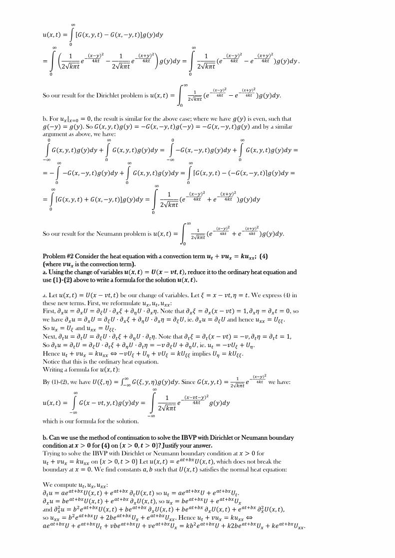
So our result for the Dirichlet problem is

.

b. For , the result is similar for the above case; where we have is even, such that

. So and by a similar

argument as above, we have:

So our result for the Neumann problem is

.

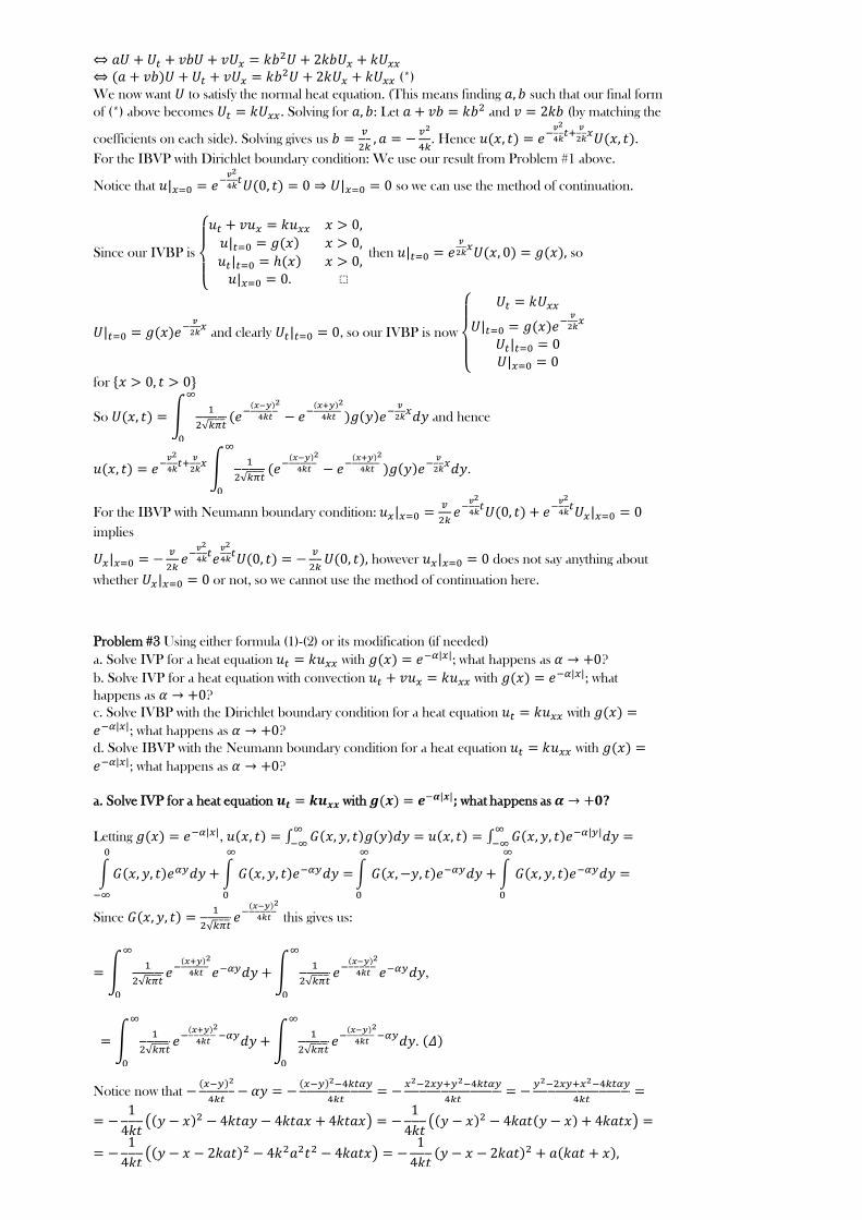
Problem #2 Consider the heat equation with a convection term ; (4) (where is the convection term).a. Using the change of variables , reduce it to the ordinary heat equation and

use (1)-(2) above to write a formula for the solution .

a. Let be our change of variables. Let . We express (4) in

these new terms. First, we reformulate :

First, . Note that , so

we have , ie. and hence .

So and .

Next, . Note that

So , ie. .

Hence implies .

Notice that this is the ordinary heat equation.

Writing a formula for :

By (1)-(2), we have

. Since

we have:

which is our formula for the solution.

b. Can we use the method of continuation to solve the IBVP with Dirichlet or Neumann boundary

condition at for (4) on ? Justify your answer.Trying to solve the IBVP with Dirichlet or Neumann boundary condition at for

on Let which does not break the

boundary at . We find constants such that satisfies the normal heat equation:

We compute :

so .

so and

so . Hence

.

(*)

We now want to satisfy the normal heat equation. (This means finding such that our final form

of (*) above becomes . Solving for : Let and (by matching the

coefficients on each side). Solving gives us

. Hence

.

For the IBVP with Dirichlet boundary condition: We use our result from Problem #1 above.

Notice that

so we can use the method of continuation.

Problem #3 Using either formula (1)-(2) or its modification (if needed)

a. Solve IVP for a heat equation with ; what happens as ?

b. Solve IVP for a heat equation with convection with ; what

happens as ?

c. Solve IVBP with the Dirichlet boundary condition for a heat equation with

; what happens as ?

d. Solve IBVP with the Neumann boundary condition for a heat equation with

; what happens as ?

a. Solve IVP for a heat equation with ; what happens as ?

Letting ,

Since

this gives us:

,

.

Since our IVBP is

then

so

and clearly , so our IVBP is now

for

So

and hence

.

For the IBVP with Neumann boundary condition:

implies

however does not say anything about

whether or not, so we cannot use the method of continuation here.

Notice now that

Hence

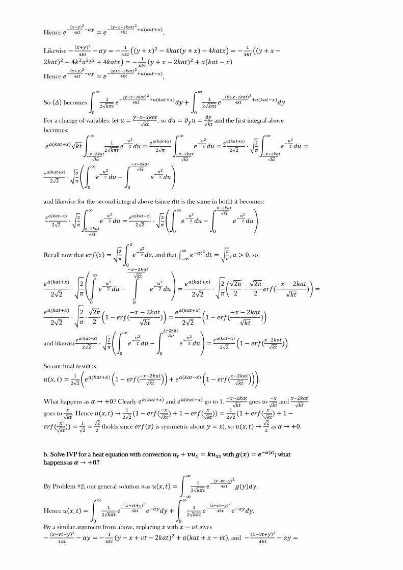
Hence

Likewise

Hence

So becomes

For a change of variables: let

, so

and the first integral above

becomes:

and likewise for the second integral above (since is the same in both) it becomes:

.

Recall now that

, and that

, so

and likewise

So our final result is

.

What happens as ? Clearly and go to 1.

goes to

and

goes to

. Hence

(holds since is symmetric about ), so

as .

b. Solve IVP for a heat equation with convection with ; what

happens as ?

By Problem #2, our general solution was

.

Hence

,

By a similar argument from above, replacing with gives

and

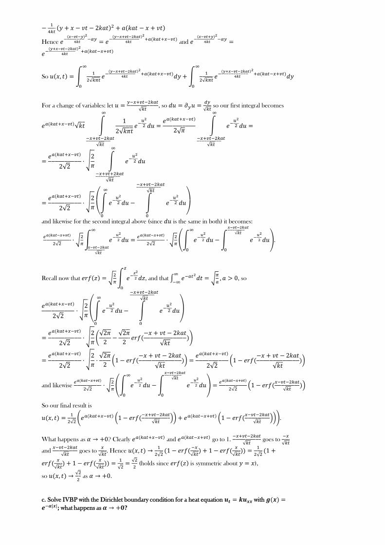
Hence

and

So

For a change of variables: let

, so

so our first integral becomes

and likewise for the second integral above (since is the same in both) it becomes:

.

Recall now that

, and that

, so

and likewise

So our final result is

.

What happens as ? Clearly and go to 1.

goes to

and

goes to

. Hence

(holds since is symmetric about ),

so

as .

c. Solve IVBP with the Dirichlet boundary condition for a heat equation with

; what happens as ?

Recall that our result for the Dirichlet boundary condition for a heat equation was

Recall that our result for the Dirichlet boundary condition for a heat equation was

. Let , so taking the odd continuation:

let

Then we have (by some manipulation similar to Problem #1) that:

and by Problem #3 part a. above we have

.

So as ,

and

,

and

.

So

Hence

as

d. Solve IBVP with the Neumann boundary condition for a heat equation with

; what happens as ?

Recall that our result for the Neumann boundary condition for a heat equation was

. Let Let , so taking the even

continuation:

let

. So our result here is identical to our result in part a,

such that

as .

Problem #4 Consider a solution of the diffusion equation in

Let

a. Does increase or decrease as a function of ?We apply the maximum principle, ie. The maximum of a function in a domain is found on the

boundary, and if a function achieves its maximum in the interior then the function is uniformly a

constant. Observe that on the boundary. Suppose , then clearly

everywhere in . If then the maximum must occur in the

boundary, so suppose otherwise. Then . By definition, must occur for some

. Hence However, this is impossible since is on the

top boundary of the rectacle and hence there. So for implies

is constant with respect to .

b. Does increase or decrease as a function of ?By a similar argument. Suppose , then . This is impossible

since is on the bottom boundary of the rectacle and hence there. So for

implies is constant with respect to .

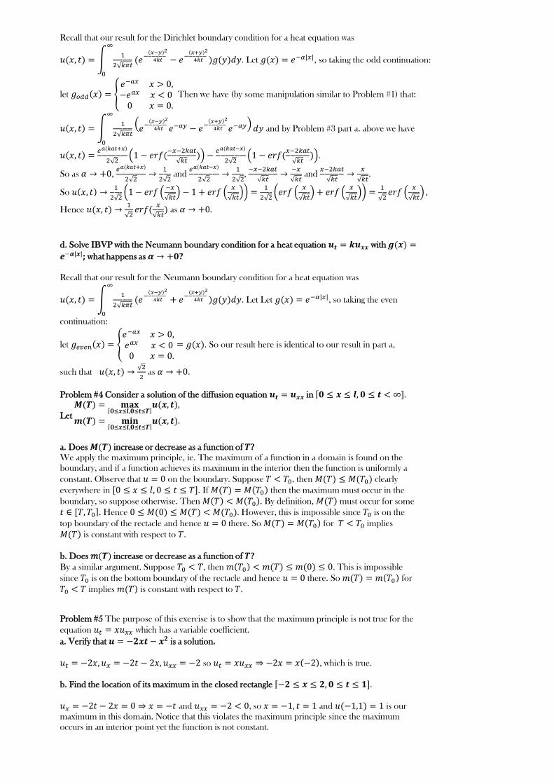
Problem #5 The purpose of this exercise is to show that the maximum principle is not true for the

equation which has a variable coefficient.

a. Verify that is a solution.

so , which is true.

b. Find the location of its maximum in the closed rectangle

and , so and is our

maximum in this domain. Notice that this violates the maximum principle since the maximum

occurs in an interior point yet the function is not constant.

c. Where precisely does our proof of the maximum principle break down for this equation?

Problem #6 a. Consider the heat equation on and prove that an energy

; (5) does not increase. Further, show that it really decreases unless

Differentiating with respect to gives

. Since

we have

. IBP here gives:

, since

given as .

Now, and implies

. Hence either

or

must hold. Hence implies

decreases, and if then does not decrease for .

c. Consider the heat equation on with the Robin boundary conditions

If and , show that the endpoints contribute to the decrease of

.

This is interpreted to mean that part of the energy is lost at the boundary, so we call the boundary

conditions radiating or dissipative.

If

, differentiating with respect to gives

. Since we have

.

IBP here gives:

. Now given

and , we have

. Hence by our results in parts a & b above,

never increases, and indeed strictly decreases if is not a constant.

b. Consider the heat equation on with the Dirichlet or Neumann boundary conditions and

prove that does not increase. Further, show that it really decreases unless

Differentiating with respect to gives

. Since

we have

. IBP here gives:

, hence:

For the Dirichlet boundary condition; ,

and for the Neumann boundary condition; . In both cases, we have

and hence

by the same reasoning in part a. So we

have virtually the same conclusion as in part a.

c. Where precisely does our proof of the maximum principle break down for this equation?

From Strauss' PDE text.

Recall that we must have for .

Notice that for the equation at the interior pt where we have a maximum, we

have that and . This means which is

impossible for .

Separation of Variables I

"Solve equation graphically" means that you plot a corresponding function and points where

it intersects with , which will give us all the frequencies ."Simple Solution" .You may assume that all eigenvalues are real (which is the case).

Problem #1 Justify examples 6--7 of Lecture 11:

Problem #1 Justify examples 6--7 of Lecture 11:

Consider the eigenvalue problem with Robin boundary conditions

with .

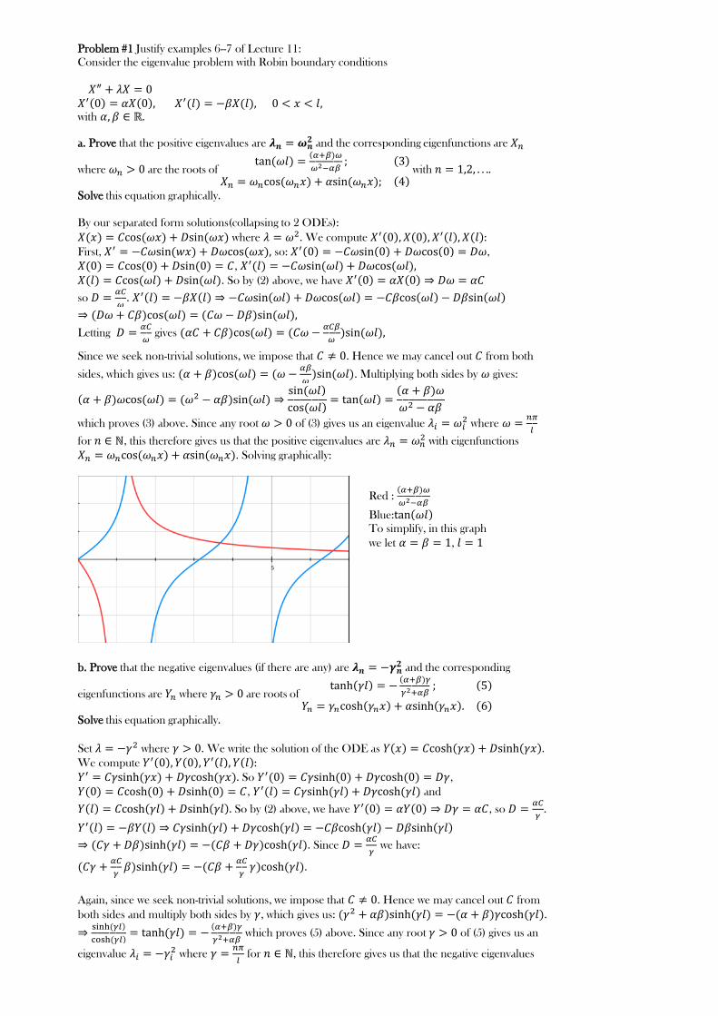
a. Prove that the positive eigenvalues are and the corresponding eigenfunctions are

where are the roots of

with .

Solve this equation graphically.

By our separated form solutions(collapsing to 2 ODEs):

where . We compute :First, so: ,

, . So by (2) above, we have

so

.

Letting

gives

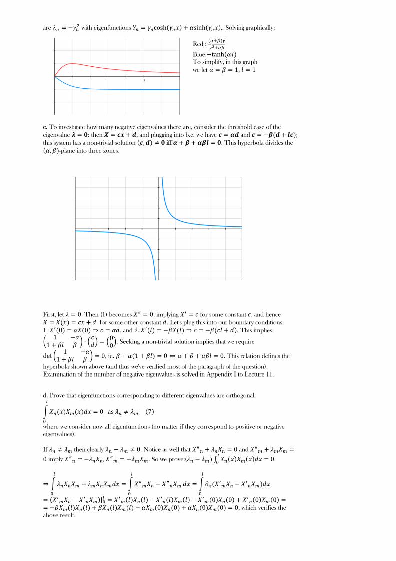
b. Prove that the negative eigenvalues (if there are any) are and the corresponding

eigenfunctions are where are roots of

Solve this equation graphically.

Set where . We write the solution of the ODE as We compute : So ,

, and

So by (2) above, we have , so

.

. Since

we have:

.

Since we seek non-trivial solutions, we impose that . Hence we may cancel out from both

sides, which gives us:

. Multiplying both sides by gives:

which proves (3) above. Since any root of (3) gives us an eigenvalue where

for , this therefore gives us that the positive eigenvalues are with eigenfunctions

. Solving graphically:

Again, since we seek non-trivial solutions, we impose that . Hence we may cancel out from

both sides and multiply both sides by , which gives us: .

which proves (5) above. Since any root of (5) gives us an

eigenvalue where

for , this therefore gives us that the negative eigenvalues

are with eigenfunctions . Solving graphically:

Red :

Blue: To simplify, in this graph

we let ,

c. To investigate how many negative eigenvalues there are, consider the threshold case of the

eigenvalue then , and plugging into b.c. we have and this system has a non-trivial solution iff . This hyperbola divides the

-plane into three zones.

First, let . Then (1) becomes , implying for some constant , and hence

for some other constant . Let's plug this into our boundary conditions:

1. , and 2. . This implies:

. Seeking a non-trivial solution implies that we require

, ie. . This relation defines the

hyperbola shown above (and thus we've verified most of the paragraph of the question).

Examination of the number of negative eigenvalues is solved in Appendix I to Lecture 11.

d. Prove that eigenfunctions corresponding to different eigenvalues are orthogonal:

where we consider now all eigenfunctions (no matter if they correspond to positive or negative

eigenvalues).

If then clearly . Notice as well that and

imply . So we prove:(

.

, which verifies the

above result.

e. Bonus Prove that eigenvalues are simple, i.e. all eigenfunctions corresponding to the same

are with eigenfunctions . Solving graphically:

Red :

Blue: To simplify, in this graph

we let ,

e. Bonus Prove that eigenvalues are simple, i.e. all eigenfunctions corresponding to the same

eigenvalue are proportional

We consider all possible cases: Case #1: . Consider two separate eigenfunctions with the same eigenvalue .

We know that positive eigenvalues have eigenfunctions and where and is a root of (3) & (4) in part

(a) above. Observe that are indeed proportional since

for some constant

, such that

, and hence proportional.

Case #2: . Consider two separate eigenfunctions with the same eigenvalue .

We know that negative eigenvalues have eigenfunctions , where and is a root of (5) & (6) in part (b)

above. Observe that are indeed proportional since

for some constant ,

such that


Case #3: . We know implies where and .Hence . Consider two separate eigenfunctions with the same eigenvalue

. Hence

for some constant ,

such that


Problem #2 Oscillations of the beam with the left end having fixed position and fixed direction and a

free right end are described by the equation: (8) with and the

boundary conditions a. Find an equation describing frequencies and corresponding eigenfunctions. (Assume all eigenvalues

are real and positive)

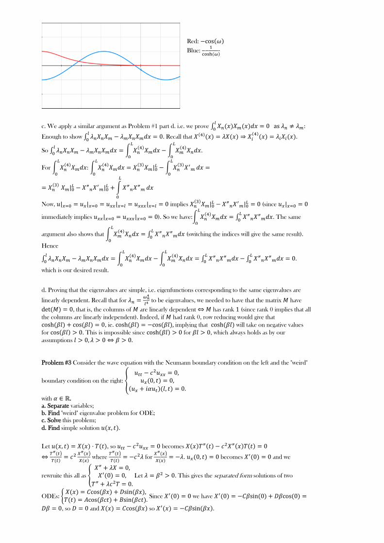
b. Solve this equation graphically.

c. Prove that the eigenfunctions corresponding to different eigenvalues are orthogonal.

d. Bonus Prove that eigenvalues are simple, i.e. all eigenfunctions corresponding to the same

eigenvalue are proportional.

a. Let , then .

, hence . Let , . Solve this ODE:

Impose the boundary conditions:

So So . So .

Hence .Now, implies .

So

and

Hence

Denote this matrix as . Showing is an eigenvalue:

We hence have a nontrivial solution for , such that:

. Hence, denote such that

. Hence

where are the roots of

Hence

Since we find :

. Solving this ODE:

Since

and hence:

, so our solution is:

b.

c. We apply a similar argument as Problem #1 part d. i.e. we prove

:

Enough to show

. Recall that

.

So

.

For

:

Now, implies

(since

immediately implies ). So we have:

. The same

argument also shows that

(switching the indices will give the same result).

Hence

.

which is our desired result.

d. Proving that the eigenvalues are simple, i.e. eigenfunctions corresponding to the same eigenvalues are

linearly dependent. Recall that for

to be eigenvalues, we needed to have that the matrix have

, that is, the columns of are linearly dependent has rank (since rank 0 implies that all

the columns are linearly independent). Indeed, if had rank 0, row reducing would give that

, ie. implying that will take on negative values

for . This is impossible since for , which always holds as by our

assumptions

Problem #3 Consider the wave equation with the Neumann boundary condition on the left and the "weird"

boundary condition on the right:

with .

a. Separate variables;

b. Find "weird" eigenvalue problem for ODE;

c. Solve this problem;

d. Find simple solution .

Let , so becomes

where

for

. becomes and we

rewruite this all as

Let . This gives the separated form solutions of two

ODEs:

Since we have

, so and so .

Red:

Blue:

b. Finding the 'weird' eigenvalue problem: becomes .

Hence

. Note then that

so

.

c. Solving this ODE:

for some constant . Hence

.

So

and for . So and

.

Hence

d.We know that the general simple solution is , so we find :

implies

.

So

is our simple solution for ,

and the general solution is

.

Fourier Series

Here Recall that the full Fourier series of on the interval is defined as:

where

,

,

for .

We use Euler's formulas:

such that:

.

Problem #1 Decompose the following into their full Fourier series on the interval :a. where ; find the "exceptional" values of ;We compute the complex form:

where

, so

Let's express this in its real form:

.

So

on the

interval and the exceptional values occur where is undefined, ie. .

b. , where ; find the "exceptional" values of ;

Let , then

. Hence since we have an expression for

for complex from the above result, we may find by letting .

So

on the interval

and the exceptional values occur where is undefined, ie.

.

c. , where ;

Let , then

. Hence since we have an expression for for

complex from the above result, we may find by letting .

Similarly for :

Let , then

. Hence since we have an expression for

for complex from the above result, we may find by letting .

So

on the interval and the

exceptional values occur where is undefined, ie.

.

So

on the interval .

Likewise for

, we have:

So

on the interval .

Problem #2 Decompose the following into their full Fourier series on the interval and sketch the

graph of the sum of such Fourier series:

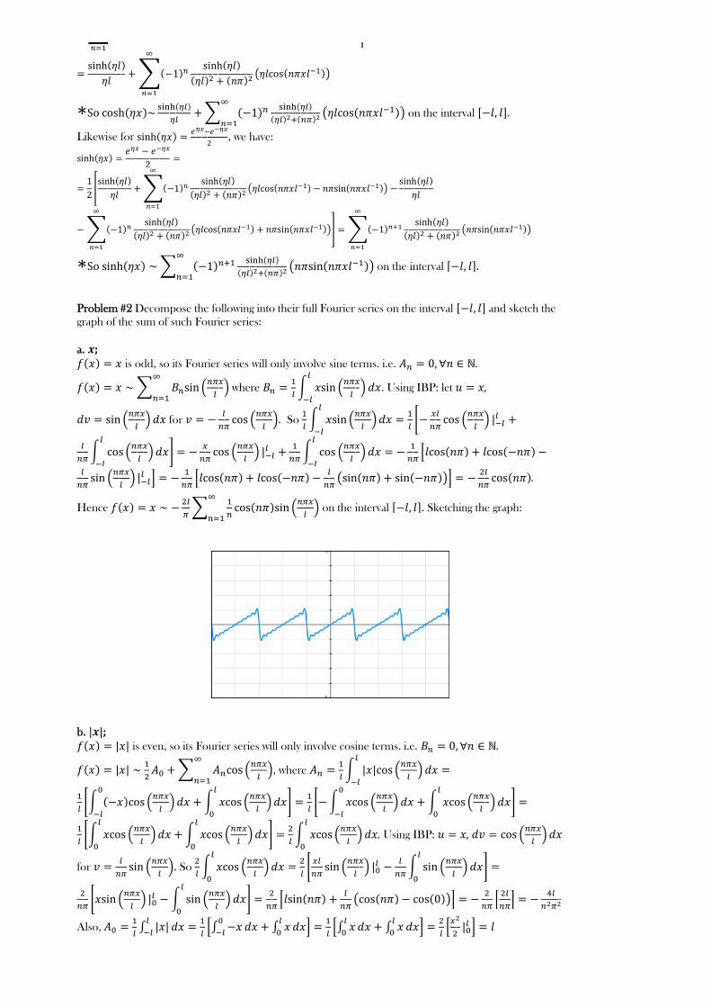
a. ; is odd, so its Fourier series will only involve sine terms. i.e. .

where

. Using IBP: let ,

for

. So

.

Hence

on the interval . Sketching the graph:

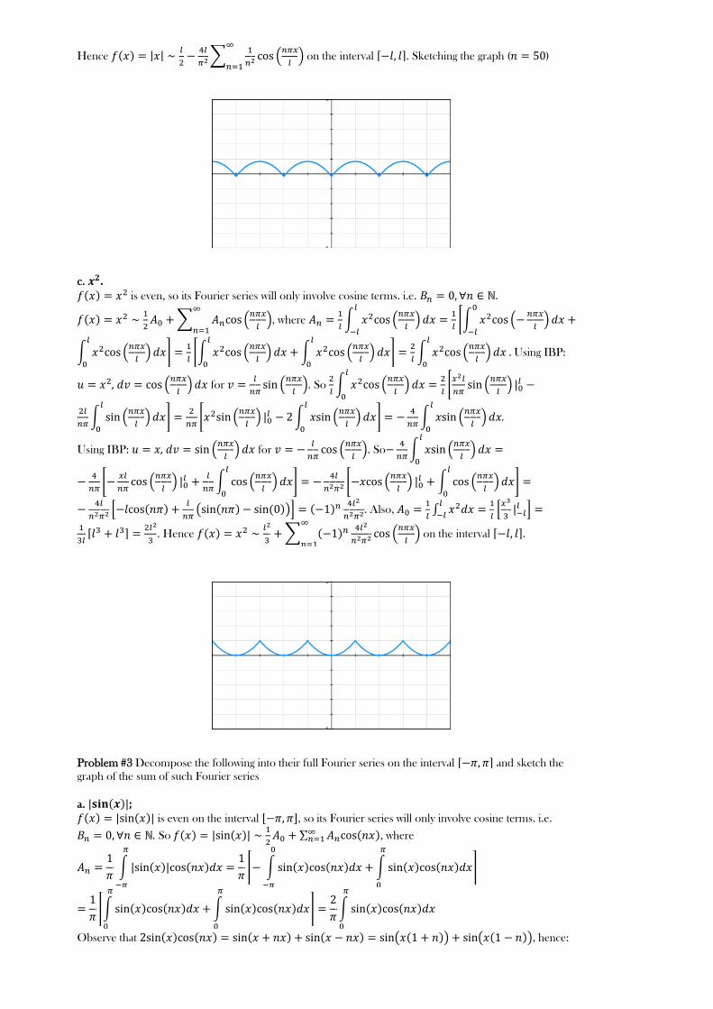
b. ; is even, so its Fourier series will only involve cosine terms. i.e. .

, where

. Using IBP: ,

for

. So

Also,

Hence

on the interval . Sketching the graph ( )

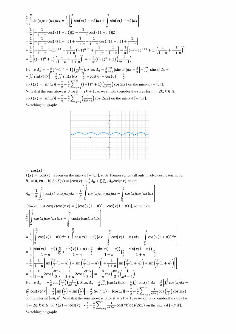
c. . is even, so its Fourier series will only involve cosine terms. i.e. .

, where

. Using IBP:

,

for

. So

.

Using IBP: ,

for

. So

. Also,

. Hence

on the interval .

Problem #3 Decompose the following into their full Fourier series on the interval and sketch the

graph of the sum of such Fourier series

a. ; is even on the interval , so its Fourier series will only involve cosine terms. i.e.

. So

, where

Observe that , hence:

Hence

on the interval . Sketching the graph ( )

Hence

. Also,

.

So

on the interval .

Note that the sum above is for , so we simply consider the cases for .

So

on the interval .

Sketching the graph:

b. ; is even on the interval , so its Fourier series will only involve cosine terms. i.e.

. So

, where

Observe that

, so we have:

Hence

. Also,

. So

on the interval . Note that the sum above is for , so we simply consider the cases for

. So

on the interval .


Problem #4 Decompose the following into their sine Fourier series on the interval and sketch the


Recall that the Fourier sine series of on an interval is given as

for

.

So for the following, let such that for

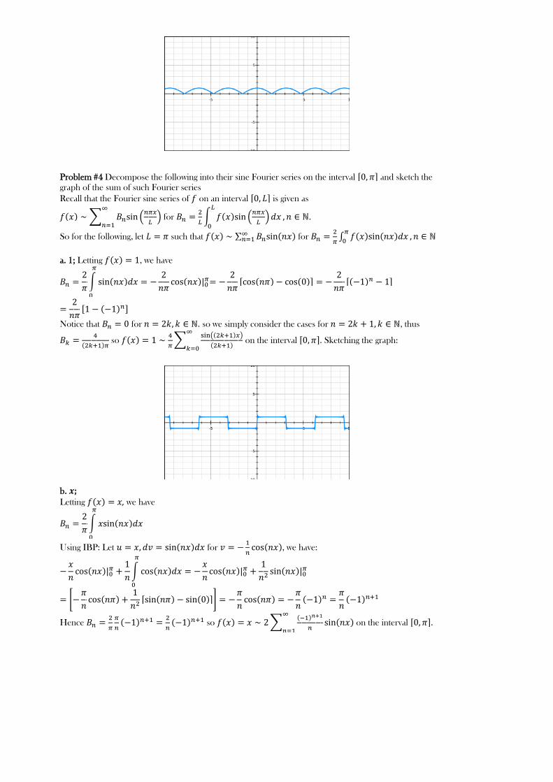
a. 1; Letting , we have

Notice that for . so we simply consider the cases for , thus

so


b. ;Letting , we have

Using IBP: Let for

, we have:

Hence

so

on the interval .

c. ;Letting , we have

We know from above that

, so using IBP:

Let

Let

,

Hence

so

on the interval .

Sketching the graph: (We include the original function superimposed)

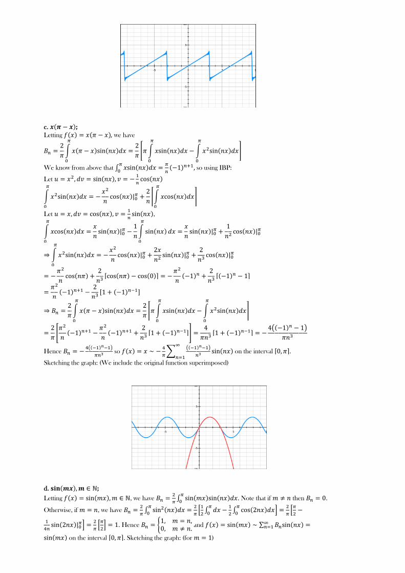
d. ;

Letting , we have

. Note that if then .

Otherwise, if , we have

. Hence

and

on the interval . Sketching the graph: (for )

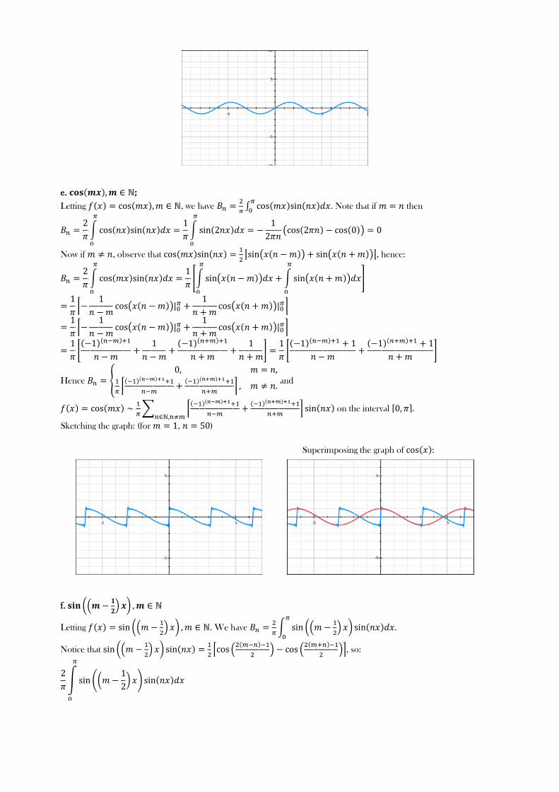
e. ;

Letting , we have

. Note that if then

Now if , observe that

, hence:

Hence

and

on the interval .

Sketching the graph: (for , )

Superimposing the graph of :

f.

Letting

. We have

.

Notice that

, so:

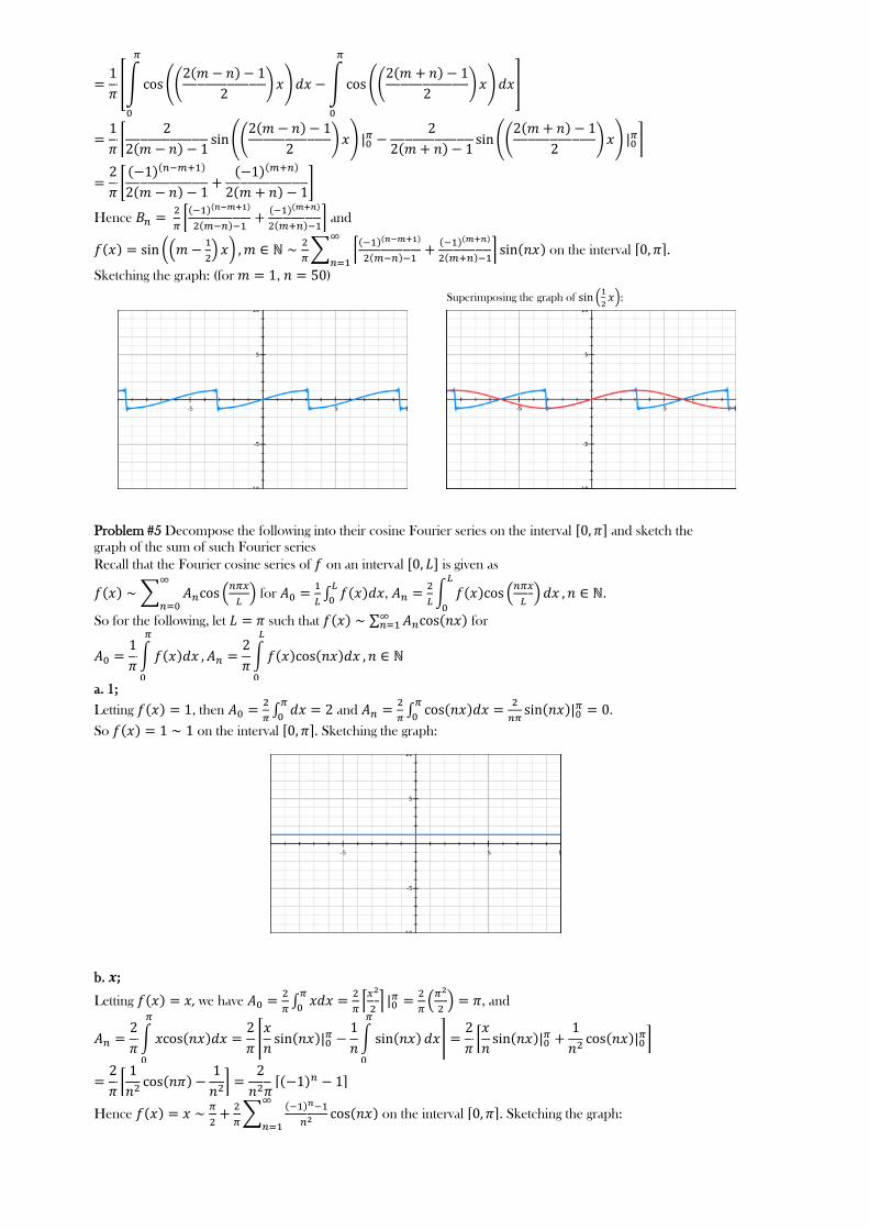
Hence

and

on the interval .

Sketching the graph: (for , )

Superimposing the graph of

:

Problem #5 Decompose the following into their cosine Fourier series on the interval and sketch the


Recall that the Fourier cosine series of on an interval is given as

for

,

.

So for the following, let such that for

a. 1;

Letting , then

and

.

So on the interval . Sketching the graph:

b. ;

Letting , we have

, and

Hence


c. ;

Letting , we have

and

We know from above that

, so we find

, using IBP:

Let

, so

Hence

and

on the interval . Sketching the graph:Superimposing the graph of :

d. ;Letting , , we have

. For , we have two cases. If , then:

If , then by 4.e. above:

So

Hence:

on the interval . Sketching the graph: (for , )

.


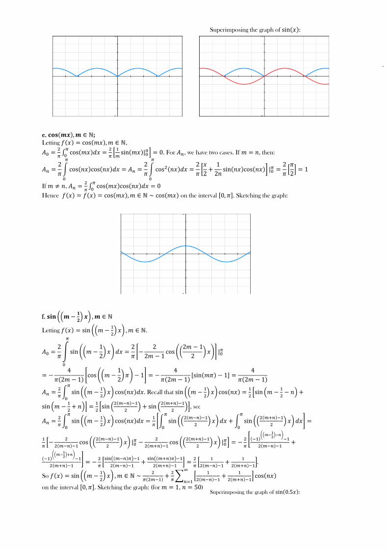
e. ; Letting ,

. For , we have two cases. If , then:

If ,

Hence on the interval . Sketching the graph:

f.

Letting

.

. Recall that

, so:

.

So

on the interval . Sketching the graph: (for , )Superimposing the graph of :

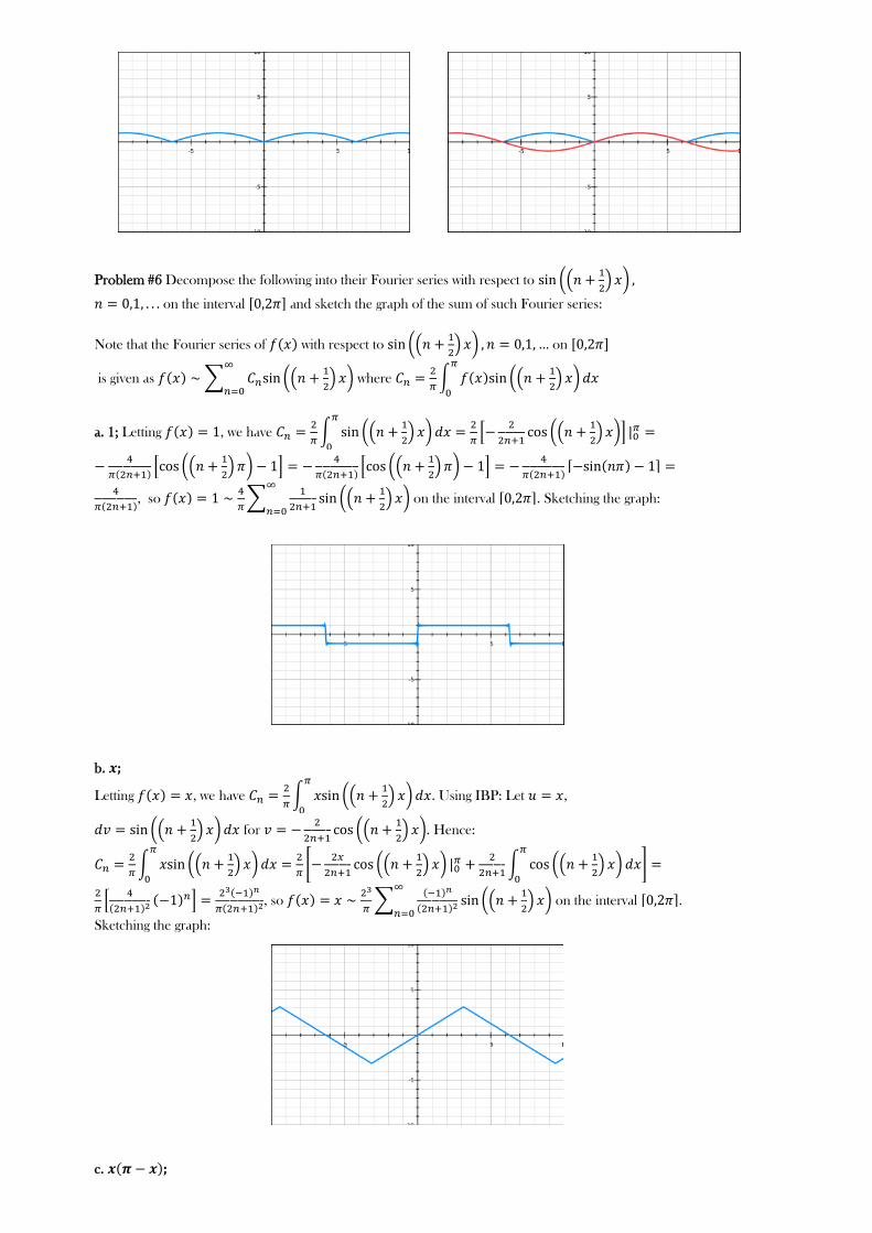
Problem #6 Decompose the following into their Fourier series with respect to

on the interval and sketch the graph of the sum of such Fourier series:

Note that the Fourier series of with respect to

on

is given as

where

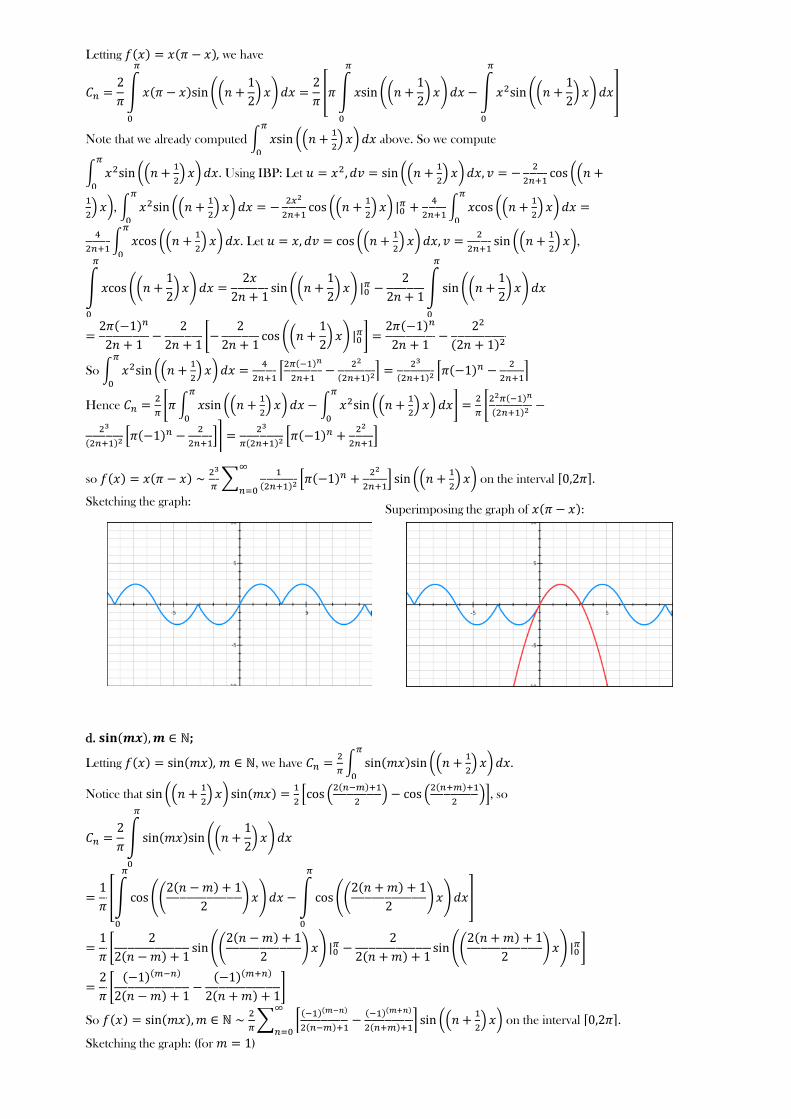
a. 1; Letting , we have

, so


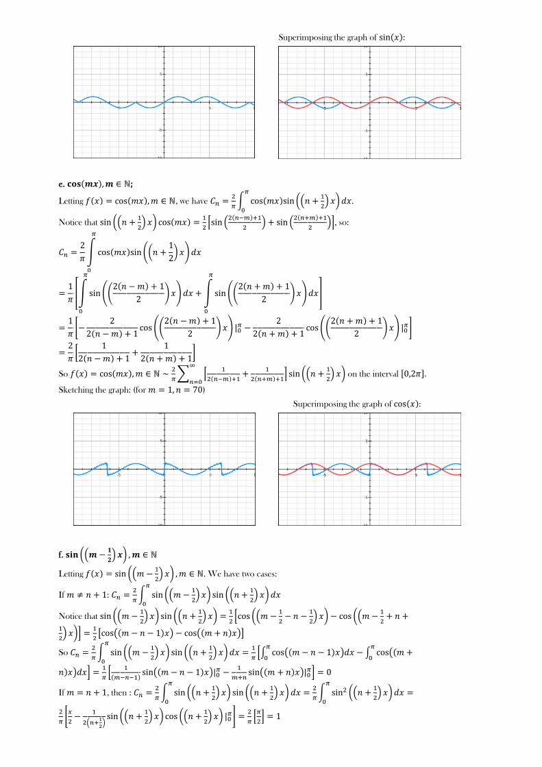
b. ;

Letting , we have

. Using IBP: Let ,

for

. Hence:

, so

on the interval .


c. ;Letting , we have

Letting , we have

Note that we already computed

above. So we compute

. Using IBP: Let

,

. Let

,

So

Hence

so

on the interval .

Sketching the graph:Superimposing the graph of :

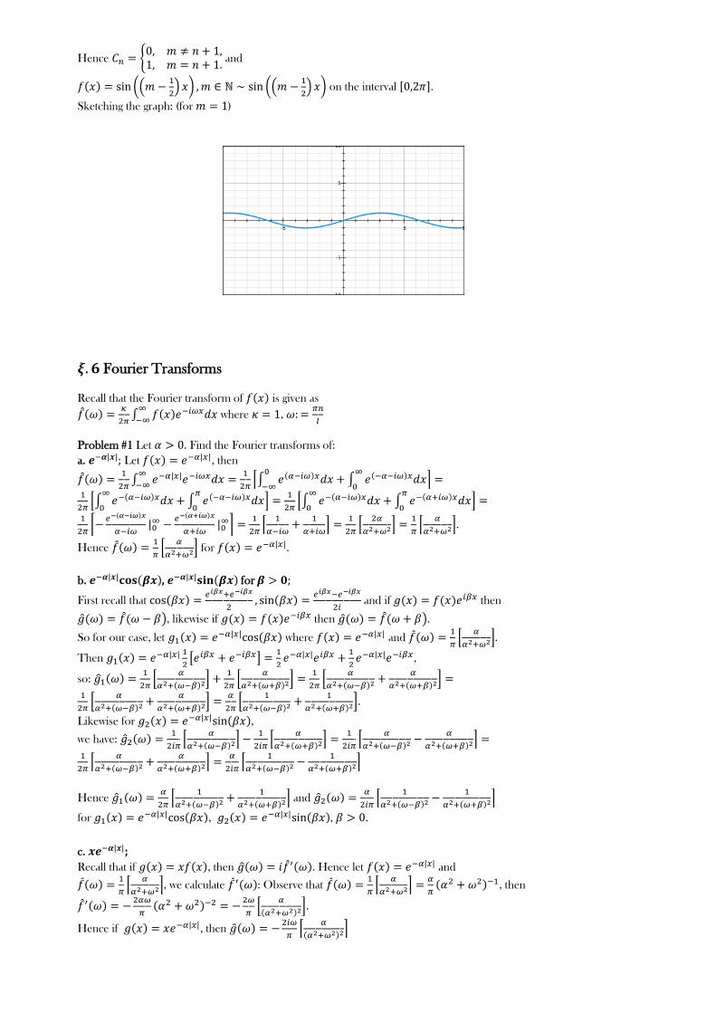
d. ;

Letting , , we have

.

Notice that

, so

So

on the interval .

Sketching the graph: (for )



e. ;

Letting , we have

.

Notice that

, so:

So

on the interval .



f.

Letting

. We have two cases:

If :

Notice that

So

If , then :

Hence

and

Hence

and

on the interval .


Fourier Transforms

Recall that the Fourier transform of is given as

where ,

Problem #1 Let . Find the Fourier transforms of:

a. Let , then

.

Hence

for .

b. , for

First recall that

and if then

, likewise if then .

So for our case, let where and

.

Then

,

so:

.

Likewise for ,

we have:

Hence

and

for , , .

c. ;

Recall that if , then . Hence let and

, we calculate : Observe that

, then

.

Hence if , then

d. , for

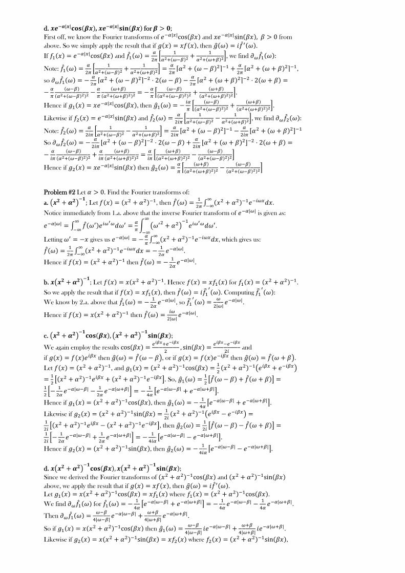
d. , for

First off, we know the Fourier transforms of and , from

above. So we simply apply the result that if , then .

If and

, we find :

Note:

,

so

.

Hence if , then

.

Likewise if and

, we find :

Note:

So

Hence if then

Problem #2 Let . Find the Fourier transforms of:

a. Let , then

.

Notice immediately from 1.a. above that the inverse Fourier transform of is given as:

.

Letting gives us

, which gives us:

.

Hence if then

.

b.

; Let . Hence for .

So we apply the result that if , then . Computing

:

We know by 2.a. above that

, so

.

Hence if then

.

c.

;

We again employ the results

and

if then , or if then .

Let , and

. So,

.

Hence if , then

.

Likewise if

, then

.

Hence if , then

.

d.

;

Since we derived the Fourier transforms of and

above, we apply the result that if , then .Let where .

We find for

.

Then

.

So if then

.

Likewise if where ,

we have

, then

we have

, then

.

Hence if then

.

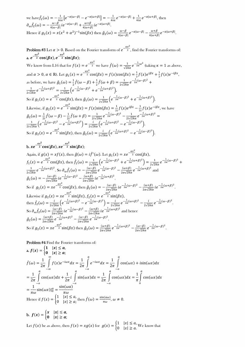
Problem #3 Let . Based on the Fourier transform of

, find the Fourier transforms of:

a.

;

We know from L16 that for

we have

(taking as above,

and , ). Let

,

as before, we have

.

So if

, then

.

Likewise, if

, we have

.

So if

, then

.

b.

;

Again, if , then . Let

,

, then

. So

and

.

So if

, then

.

Likewise if

,

,

then

.

So

and hence

.

So if

then

.

Problem #4 Find the Fourier transforms of:

a.

Hence if

then

, .

b.

Let be as above, then for

We know that

, , so we apply the result that if then .

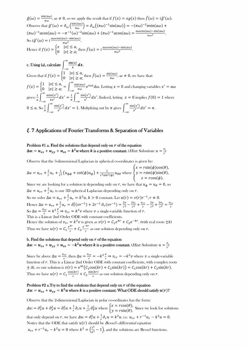
, , so we apply the result that if then .

Observe that

.

So

.

Hence if

then

.

c. Using (a), calculate

.

Given that if

then

, , we have that:

. Letting and changing variables

gives:

. Indeed, letting implies where

. So

. Multplying out by gives

.

Applications of Fourier Transforms & Separation of Variables

Problem #1 a. Find the solutions that depend only on of the equation

where is a positive constant. (Hint: Substitute

)

Observe that the 3-dimensional Laplacian in spherical co-ordinates is given by:

where

Since we are looking for a solution depending only on , we have that , so

is our 3D spherical Laplacian depending only on .

So we solve

, constant. Let .

Hence

So

where a single-variable function of .

This is a Linear 2nd Order ODE with constant coefficients.

Hence the solution of is given as

. (with real roots )

Thus we have

as our solution depending only on .

b. Find the solutions that depend only on of the equation

where is a positive constant. (Hint: Substitute

)

Since by above

, then

where a single-variable

function of . This is a Linear 2nd Order ODE with constant coefficients, with complex roots

, so our solution is .

Thus we have

as our solution depending only on .

Problem #2 a.Try to find the solutions that depend only on of the equation

where is a positive constant. What ODE should satisfy ?

Observe that the 2-dimensional Laplacian in polar co-ordinates has the form:

where

Since we look for solutions

that only depend on , we have

. i.e. .

Notice that the ODE that satisfy should be Bessel's differential equation

where

, and the solutions are Bessel functions.

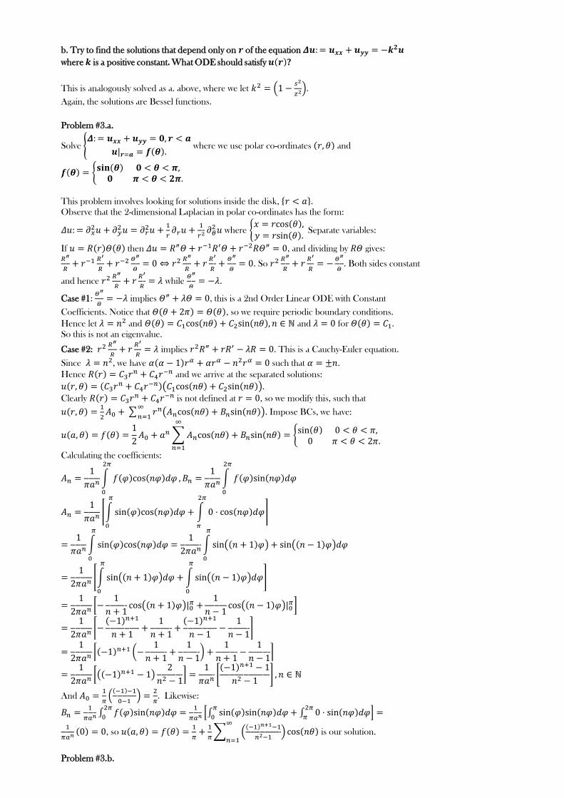
b. Try to find the solutions that depend only on of the equation

where is a positive constant. What ODE should satisfy ?

This is analogously solved as a. above, where we let

.

Again, the solutions are Bessel functions.

Problem #3.a.

Solve

where we use polar co-ordinates and

This problem involves looking for solutions inside the disk, .Observe that the 2-dimensional Laplacian in polar co-ordinates has the form:

where

Separate variables:

If then , and dividing by gives:

. So

. Both sides constant

and hence

while

.

Case #1:

implies , this is a 2nd Order Linear ODE with Constant

Coefficients. Notice that , so we require periodic boundary conditions.

Hence let and and for .

So this is not an eigenvalue.

Case #2:

implies . This is a Cauchy-Euler equation.

Since , we have such that .

Hence

and we arrive at the separated solutions:

.

Clearly

is not defined at , so we modify this, such that

. Impose BCs, we have:

Calculating the coefficients:

And

. Likewise:

, so

is our solution.

Problem #3.b.

Solve


Solve


Here we're looking for solutions outside the disk.

We proceed as in the solution of#3.a. up to the end of Case #2, where we have

Make the following changes of variables, and subsequently, changes in domains:

Change

, such that

. So as

.

Hence the above becomes, after imposing the BCs:

With coefficients given as:

Just as above,

, so

. Likewise,

So

is our solution.

Problem #4.a.

Solve



Differentiating this expression w.r.t. and imposing the BC gives:

, so is:

Observe that

.

Hence has one free coefficient and we may find a unique solution up to a constant .

Calculating the coefficients at :

Using a derivation similar to #3.a. above:

And undefined (indeed, we omit it for our constant term above).

Hence

is our solution, for some constant .

Problem #4.b.

Solve


Solve


Here we're looking for solutions outside the disk.

(If you look it up, this is solved in a simpler way using something called the "Poisson Kernel".)


,

As in #4.a., differentiating this expression w.r.t. gives:

Observe that

.

Hence has one free coefficient and we may find a unique solution up to a constant .

So our solution for the Neumann problem on the interior is of the form:

as derived in #4.a.

Make the following changes of variables, and subsequently, changes in domains:

Change

, such that

. So as

.

Hence the above becomes

.

Impose the BCs: We find at the boundary

(and indeed, after our change of variables, our boundary condition becomes

):

And our coefficients are given by:

Again, we employ our derivation from #3.a., giving:

And undefined (indeed, we omit it for our constant term above).

Hence

, i.e.

for some constant .

The Laplacian

Problem #1.1. Find the solutions that depend only on of the equation

Observe that the 2-dimensional Laplacian in polar co-ordinates has the form:

where

Since we look for solutions

that only depend on , we have

. i.e. .

Multiplying out by gives . Notice then that .

So implies for some constant . Hence

. Solving gives:

, and so for arbitrary constants .

, and so for arbitrary constants .

2. Find the solutions that depend only on of the equation .

Observe that the 3-dimensional Laplacian in spherical co-ordinates is given by:

where

(From substituting

)

Since we are looking for a solution depending only on , we have that , so

is our 3D spherical Laplacian depending only on .

Multiplying out by gives . Notice though that

. So

implies for some constant .

Hence

. Solving gives:

for constant, i.e.

for arbitrary constants .

3. (Bonus) In the -dimensional case, prove that if with

then

.

Notice that

for .

First off, note that

, hence

.

thus

.

So

and hence

which proves the statement.

4. (Bonus) In the -dimensional case, prove (for ) that satisfies the Laplace

equation for iff .

Suppose satisfies

for , . Approaching similarly

to part 1. and 2. above: multiplying out by gives . Notice

though that

, so implies

for some constant . Since we impose we may let .

Hence , which is solved as for some constant . This

proves the forward direction.

Using characterized above, we find and show that satisfies

.

Let , and . Then and

. So

. So satisfies the Laplace

equation.

Problem #2

Using the proof of the Mean Value Theorem (S4.L24), prove

1. (The Subharmonic Mean-Value Property)

If in , then does not exceed the mean value of over the sphere bounding this ball:

Suppose in and is . We must have that

We claim that

is an increasing function of as .

This would imply that

for .

Consider the following a review:

Let be an arbitrary bounded domain (i.e. a ball), with boundary .

Let be a volume element (think in ), an area element (think in ),

and a unit exterior normal to . Let be a vector field and its divergence.

By the Divergence Theorem, we have:

That is, the rate of fluid flowing out of the region is equivalent to adding up the sources of flow

inside the region and subtracting the sinks. i.e. Integrating the field's divergence over the interior of

the region should equal the integral of the vector field over the region's boundary.

Since , , we take and .

If , we know , so

Let's invoke polar co-ordinates. where is an area element on the unit sphere

expressed in terms of co-ordinates on its surface.

So the average is

which lets us differentiate.

Since , we have:

Hence for

, we have:

This immediately proves our assertion from the first paragraph above.

2. (The Superharmonic Mean-Value Property)

does not exceed the mean value of over this ball :

Observe that

,

Now, since

from part 1, we have:

So

.

Problem #3

1. Using the proof of the maximum principle, prove the maximum principle for subharmonic

functions (max-sub) and the minimum principle for superharmonic functions (min-sup).

Recall that is subharmonic in domain if .

Let and .Suppose has a maximum in at the interior point . Hence

and

. Thus

. Now observe

implies . .

Hence has no interior maximum in .

Since continuous, it must achieve a maximum on the closure of . Suppose it is achieved on the

boundary at the point . Hence for all ,

,

where is the largest distance from to the origin. i.e.

Since this holds for all , letting gives

for all .

Since this holds for all , letting gives

for all .

Now, this maximum is attained at some point .

Hence for all .

Recall that is superharmonic in domain if .

Let . By above, is subharmonic and attains its maximum on . This is equivalent to a

minimum for . Hence attains its minimum on .

2. Show that the minimum principle for subharmonic functions (min-sub) and the maximum

principle for superharmonic functions (max-sup) do not hold (do not exist).

A counterexample (min-sub): Let . The min of is and is attained at the

point . Now let . If the min-sub principle were to hold,

the minimum of should occur at , where .

This implies such that is subharmonic.

However, at the point , , and for any we have .

This means that the minimum is attained at which is an interior point. .

A counterexample (max-sup): Let . The max of is and is attained at the

point . Now let . If the max-sup principle were to

hold, the minimum of should occur at , where .

This implies such that is superharmonic.

However, at the point , , and for any we have .

This means that the maximum is attained at which is an interior point. .

3. Prove that if are respectively harmonic, subharmonic and superharmonic functions in

the bounded domain , and that they all coincide on (such that ), then

in .

If is harmonic and is subharmonic, with the same boundary value such that

is subharmonic. Then, by the maximum principle,

and hence

. Likewise, if is harmonic and is superharmonic, with the same boundary value

such that is superharmonic. Then, by the minimum principle,

and hence .

Hence in .

Problem #4 (Bonus)

Using the Newton Shell Theorem, prove that if the Earth was a homogeneous solid ball, then the

gravity pull inside of it would be proportional to the distance to the centre.

The Newton Shell Theorem can be found in the notes for L25.

In , suppose we had a spherically symmetric density . Let be the Earth's radius.Then:

1. If the density is concentrated as then inside of the Earth's cavity , the pull is .

2. If the density is concentrated as then in , the pull would be as if it was created

by the same mass but concentrated in the centre.

Therefore the outer layers have no pull, and the interior layers have a pull of

. In particular, travelling to the centre of the Earth in this model would

involve us experiencing decaying gravity.

Suppose we drill a tunnel and drop something down. The acceleration of the object would be

where is the acceleration due to gravity on the Earth's surface,

.

And the time it takes to drop through to the centre is:

Thus, the distance to the centre is

where is our velocity.

Indeed, our speed is

, so the distance to the centre is .

Laplace's Equation and Potential Theory

Problem #1 Find a function harmonic in and coinciding with as

.

Recall that the Laplace equation in spherical co-ordinates is given by

Recall that the Laplace equation in spherical co-ordinates is given by

where

. Assume separable solutions. Let .

Hence (i.e. harmonic) implies

.

Dividing out by

gives:

. The former and latter expressions

depend solely on and respectively, so both are constant:

, so:

is an Euler ODE, , which has solutions iff By our hint, since we are in spherical co-ordinates (in a ball), the solution must be infinitely

smooth in the centre, which is possible iff s.t. must be a polynomial of .i.e. must be a harmonic polynomial of degree depending only on and .

By the hint, let and determine :

After some calculation:

, and

We impose , such that:

, ,

. Now let , such that:

This simplifies to .

Consider when , this implies

st

By our assumption, this means

and .

Notice as well that these coefficients still apply for even if .

Hence our solution for harmonic in coinciding with on

is

.

Problem #2 Apply the 'method of descent' to the Laplace equation in , and starting from

'Coulomb Potential in 3D',

, derive

'Logarithmic potential in 2D',

.

Let

.

Let

.

Notice that does not depend on the third spatial variable , so

By the hint:

(where appears as the sphere covers the disk twice). So:

Calculating the expression in parentheses:

Notice that

,

hence:

So

, which derives logarithmic potential in 2D.

Problem #3 Using the method of reflection, construct a Green function for:

a. Dirichlet problem for the Laplace equation on the half plane and half space respectively.

b. Neumann problem for the Laplace equation on the half plane and half space respectively.

1. The Dirichlet problem for the upper half plane is given by:

Note that in the whole plane, the Green function is the potential

where , .

Consider then the half plane , so our boundary is

where we have our boundary condition . By the method of reflection,

consider , and let be its reflection about the boundary .

Since we require our Green function to be identically on the boundary, we add the term

to the Green function on the whole

plane, so that where . So in general, for we have:

where , , .

2. The Dirichlet problem for the upper half space is given by:

Note that in the whole space, the Green function is the

potential

where ,

. Proceeding in a similar manner as above: for the half-space

, our boundary is . By the method

of reflection, consider , and let be its reflection

about the boundary . Since we require our Green function to be identically on the

boundary, we add the term

such that where . So in general for we have:

. i.e.

where as above.

3. The Neumann problem for the upper half plane is given by:

Note that in the whole plane, the Green function is the potential

where , .

Consider then the half plane , so our boundary is

where we have our boundary condition . By the method of

reflection, consider , and let be its reflection about the

boundary . Since we require on the boundary, we add the term

to the Green function on the whole plane,

so that where . Verifying this:

Thus imposing gives , so in general, for we have:

where , , .

4. The Neumann problem for the upper half space is given by:

Note that in the whole space, the Green function is the

potential

where ,

. Proceeding in a similar manner as above: for the half-space

, our boundary is . By the method

of reflection, consider , and let be its reflection

about the boundary . Since we require on the boundary, we add the term

such that where . Verifying this:

Thus imposing gives , so in general for we have:

. i.e.

where as above.

Problem #4 Apply the method of descent to find the stationary solution of

(instead of a non-stationary solution) of

Start from Kirchhoff's formula and derive it for with is the potential on the whole

space,

.

Recall that Kirchhoff's formula is given by:

Recall that Kirchhoff's formula is given by:

.

For our case, we have and a stationary solution has and doesn't depend on . So we have:

Let so

and by the method of descent:

Letting

, the above becomes

, and since , we have that:

is our stationary solution for the problem.

Functionals, Extremums, Variations and Distributions.

Problem #1 Consider the variational problem under constraint:

With boundary conditions

a. Write down the Euler-Lagrange equation .

Recall that if

is a functional, then is the Lagrangian.

So for

,

. Hence, we have by definition:

Note then that , so we have that the Euler-Lagrange equation is:

. Multiplying out the negative gives the

EL-equation as .

Likewise for

, we have

and:

.

Hence is our Euler-Lagrange equation for the problem.

b. Under the boundary conditions, solve it and find out eigenvalues for each solution exists.

Our eigenvalue problem is . The Cauchy-Euler equation for this 4th Order ODE

is: , and the roots are: . Let .

Then . Recall our hint: changing the interval from to

will not change the boundary conditions nor the ODE (which are symmetric, i.e. survives

) then we can consider even and odd eigenfunctions separately.

Then: .

Finding the even eigenfunctions (where is even): . Impose the BCs:

Hence . Thus are our eigenvalues.

Finding the eigenfunctions: implies .

If , implies , , so in general , and our

eigenfunctions are for .

Finding the odd eigenfunctions (where is odd): . Impose the BCs:

Since they are equal, we equate them: , implies .

Since they are equal, we equate them: , implies .

So graphically, the eigenvalues are where the graphs of and intersect (as functions of ).

Problem #2 Consider the variational problem:

,

where .

a. Write down the Euler-Lagrange equation.

Given above, the Lagrangian is

.

So and the Euler-Lagrange Equation is:

, i.e.

.

b. Write down all of its boundary conditions.

Recall that

Let . By part a. above, we have:

Now recall:

where is an area element and is a unit interior normal to . Thus, we have:

where is an inner normal.

Notice that Let's specify what the inner normals are for each case. Geometrically:

Designate cases #1 to #4 as respectively. This gives us:

where , s.t. on and on , corresponding to the top and bottom of the square, and the left and right sides, respectively.

Given that there is no constraint on the border, we have for all .

This gives us the boundary conditions: and no boundary

condition at .

Case #1: . The inner normal here is the vector (in red).

Case #2: . The inner normal here is the vector (in blue). These are the left and right sides of the square.

Case #3: . The inner normal here is the vector (in green).

Case #4: . The inner normal here is the vector (in yellow). These are the top and bottom of the square.

Problem #4 Find the Fourier transform of , (Heaviside function).

Let

be the Heaviside function.

Finding the Fourier transform by definition, we have:

Notice that

for all , then:

To properly compute this limit, consider the term .

Express this in polar form:

.

Observe now:

.

Since arctan is odd, this becomes:

.

So

.

(We employed the fact that

).

Hence

.

Differentiate both sides by gives:

.

So

.

Since

has a singularity at , we must thus take the Cauchy principal value of the integral.

Hence,

and so:

is the Fourier transform of , the Heaviside function.

Problem #3 Consider distributions now. Calculate right from the definition:

a. We first find and then compute the above product.

Recall that for an arbitrary test function. Then by definition:

and .Now recall that the product of a distribution by a function is defined as:

for

or

and .

Hence let , , then .By some computation, this gives us: .

Thus .

b. Proceeding similarly as above:

.

Thus .

c. Let's first compute .

.

Hence, . By some computation, this gives us:

.Thus .

Problem #5 Consider the wave equation: on , where

and

.

a. Write down the wave equation for and separately.

a. Write down the wave equation for and separately.

as .

b. Find out transmission conditions (there must be 2 of them) linking:

.

We require that be a function, not a distribution. This implies that be continuous at , such

that is differentiable at . So our first condition is .

Next, the solution must not have shocks. Clearly a shock would occur if

. That is, approaching from the left or the right of gives a

singularity. Hence we require

and that these limits are equal.

i.e. . This is our second condition.

Documents

Problems in Partial Differential Equations