Problem-solving environments for biological morphogenesis

Problem-Solving Environments for Biological MorphogenesisRoeland M.H. Merks, Alfons G. Hoekstra, Jaap A. Kaandorp, Peter M.A. Sloot, and Paulien Hogeweg

Citation: Computing in Science & Engineering 8, 61 (2006); doi: 10.1109/MCSE.2006.11 View online: http://dx.doi.org/10.1109/MCSE.2006.11 View Table of Contents: http://scitation.aip.org/content/aip/journal/cise/8/1?ver=pdfcov Published by the AIP Publishing Articles you may be interested in Problem-Solving Methods for Understanding Process Executions Comput. Sci. Eng. 10, 47 (2008); 10.1109/MCSE.2008.78 Student Problem-Solving Behaviors Phys. Teach. 44, 250 (2006); 10.1119/1.2186244 Time to completion reveals problemsolving transfer AIP Conf. Proc. 790, 205 (2005); 10.1063/1.2084737 Computer ProblemSolving Coaches AIP Conf. Proc. 790, 197 (2005); 10.1063/1.2084735 Problem-solving challenges Phys. Teach. 37, 161 (1999); 10.1119/1.880203

This article is copyrighted as indicated in the article. Reuse of AIP content is subject to the terms at: http://scitationnew.aip.org/termsconditions. Downloaded to IP:

142.132.1.147 On: Thu, 11 Sep 2014 18:30:17

http://scitation.aip.org/content/aip/journal/cise?ver=pdfcov

http://scitation.aip.org/search?value1=Roeland+M.H.+Merks&option1=author

http://scitation.aip.org/search?value1=Alfons+G.+Hoekstra&option1=author

http://scitation.aip.org/search?value1=Jaap+A.+Kaandorp&option1=author

http://scitation.aip.org/search?value1=Peter+M.A.+Sloot&option1=author

http://scitation.aip.org/search?value1=Paulien+Hogeweg&option1=author

http://scitation.aip.org/content/aip/journal/cise?ver=pdfcov

http://dx.doi.org/10.1109/MCSE.2006.11

http://scitation.aip.org/content/aip/journal/cise/8/1?ver=pdfcov

http://scitation.aip.org/content/aip?ver=pdfcov

http://scitation.aip.org/content/aip/journal/cise/10/3/10.1109/MCSE.2008.78?ver=pdfcov

http://scitation.aip.org/content/aapt/journal/tpt/44/4/10.1119/1.2186244?ver=pdfcov

http://scitation.aip.org/content/aip/proceeding/aipcp/10.1063/1.2084737?ver=pdfcov

http://scitation.aip.org/content/aip/proceeding/aipcp/10.1063/1.2084735?ver=pdfcov

http://scitation.aip.org/content/aapt/journal/tpt/37/3/10.1119/1.880203?ver=pdfcov

JANUARY/FEBRUARY 2006 61

C O M P U T A T I O N A LB I O L O G Y

Biologists traditionally use back-of-the-envelope, arrow-and-box-type concep-tual models of biological growth andform mechanisms to develop hypothe-

ses and design experiments. Following the intro-duction of experimental, high-throughputtechniques (such as DNA sequencing), the num-ber of known interacting biological factors hasgrown so rapidly that such “mental juggling” of bi-ological data is no longer feasible; conceptualmodels must be replaced by computational mod-eling. Developing and using the tools needed forsuch computational studies of biological growthand development requires extensive training andknowledge typically unavailable to research biolo-gists. Given this, mathematicians, physicists,computer scientists, or computationally trained bi-ologists typically conduct such studies—and in-evitably spend the majority of their time in codeand algorithm development.

Problem-solving environments aim to addressthis problem.1 PSEs are software environments thathide the simulation code’s implementation details,letting users formulate their problems at higher ab-straction levels in the target problem’s language.Moreover, PSEs often contain simulation systemknowledge, and can thus advise and warn usersabout their chosen parameters. PSEs thereforemake it possible to separate technical work on thesimulation codes and methods from conceptualcomputational experimentation and analysis.

Given its modular nature, biological morpho-genesis—the reorganization of embryonic cells andtissues into a well-organized embryo recognizableas the adult or larva—is particularly well suited forPSEs. Ideally, a morphogenesis PSE would

• implement the biological and physical behaviorof single modules, such as cells or organs;

• provide the infrastructure for them to interact;and

• offer the tools necessary to transparently set upsimulations on parallel architectures and visual-ize and analyze the resulting structures.

We developed two PSE prototypes for studyingbiological morphogenesis. Our coral-growth PSEenables coral-growth model construction usinghigh-level objects, including polyps, coral skele-tons, and boundary and initial conditions. By in-

Problem-Solving Environments for Biological Morphogenesis

Simulation is an important tool for understanding developmental mechanisms, but thetechnology is often too complex for biologists lacking higher computational skills. Using atiered architecture, the developers of these problem-solving environment (PSE) prototypesensure accessibility for users at all skill levels.

ROELAND M.H. MERKS, ALFONS G. HOEKSTRA, JAAP A. KAANDORP, AND PETER M.A. SLOOT

University of AmsterdamPAULIEN HOGEWEG

Utrecht University

1521-9615/06/$20.00 © 2006 IEEE

Copublished by the IEEE CS and the AIP


142.132.1.147 On: Thu, 11 Sep 2014 18:30:17

62 COMPUTING IN SCIENCE & ENGINEERING

cluding such conceptual objects as independentmodules, the user can easily specify the simulationsetup. This modular architecture also encouragesa multimodel approach in which researchers cancompare different models and solutions to arrive ata satisfying solution. Our PSE for multicellular de-velopment uses an evolutionary algorithm to findinteresting developmental mechanisms by analyz-ing thousands of specimens. The PSE hides theevolutionary algorithm’s parallel implementationfrom users, but allows low-level additions andmodifications to the specimen development algo-rithms and fitness functions. Here, we describeeach prototype in detail, and discuss their implica-tions and potential.

Biological Morphogenesisand ComputingMost multicellular organisms start life as tiny,spherical, fertilized egg cells. How the adult organ-ism’s intricate shape then unfolds is one of biology’smost fundamental and fascinating challenges.While popular wisdom holds that an adult organ-ism’s every property is “in the genes,” the scientificcommunity realizes that biological form developsin an intricate interaction between physical pattern-formation processes and genetic regulation.

In his seminal 1917 book, On Growth and Form,D’Arcy Thompson discussed how we could under-stand the shape of biological structures—includingcell aggregates, beehives, sea shells, or jelly fish—by comparing them to simple physical and mathe-matical patterns, such as soap froths, oil drops onwater, and logarithmic spirals. Alan Turing’s 1952classic, The Chemical Basis of Morphogenesis, firmlypositioned computational and theoretical methodsas essential pillars, alongside experimental ap-proaches, of biological pattern formation study.

With the availability of powerful computers, wecan now explore the interplay between physicalpatterning and genetic information in much moredetail. By building a computational environmentthat reproduces an organism’s development, we candistill the set of essential physical and biological in-teractions from the tangle of biological develop-ment processes. Five years ago, Stan Marée fromUtrecht University, the Netherlands, demonstratedthat this “computing an organism”2 approachshould be liberated from the realm of science fic-tion. Using a hybrid of a partial differential equa-tion and Metropolis cellular automata, Maréereconstructed all the transformation stages in thecellular slime mould Dictyostelium discoideum, fromsingle cells to fruiting body.3

Marée applied one of the many simulation

methods for biological growth and form that sci-entists have developed over the past few decades.4

At the University of Calgary, for example, the Al-gorithmic Botany group’s Virtual Laboratory(http://algorithmicbotany.org/virtual_laboratory)provides an extensive environment to describe andvisualize plant growth with Lindenmayer systems(L-systems). Introduced by Aristid Lindenmayerin 1968, L-systems are rewriting grammars thatreflect plant growth’s inherent recursivity: shootsgrow from buds, while buds grow on shoots. L-systems have been widely applied in both biol-ogy and computer graphics. Another, morerecently introduced morphogenesis PSE is Com-puCell3D,5 a 3D simulation framework that fa-cilitates multicellular morphogenesis simulationsby letting users specify cell properties using XML.These PSEs focus primarily on setting up singlemorphogenesis simulations on single processors.Morphogenesis simulations often need more pow-erful, parallel architectures, either because simu-lating a single biological specimen and itsenvironment is computationally demanding, orbecause we need numerous small simulations tocarry out efficient searches through numerouspossible model outcomes. However, researchersrarely contend with the challenge of making sucharchitectures accessible to experimental biologists,while also keeping them flexible enough for moreexperienced users. As we now describe, our PSEprototypes address this problem using modular,tiered architectures.

The Coral Growth PSEStony corals are colonies of polyps—tiny seaanemones—that live on a calcium carbonate skele-ton that they deposit in layers. Growing severalcentimeters a year, corals can form myriad shapes,from flat, stone-covering crusts to huge hemi-spheres to branching structures. Although many bi-ologists argue that such formations involveintricate, genetically controlled communication be-tween the polyps, in some cases, the corals’ branch-ing shapes can be explained with very simplemechanisms that assume polyps are “individualists”that don’t actually communicate at all.

Using computer modeling, we’ve shown that wecan obtain realistic branching shapes if we assumethat polyps determine the velocity of skeleton de-posits on the basis of how much food they consumefrom the surrounding water.6–8 Such models thussuggest a physical mechanism for at least somecorals’ shape development. Coral biologists, whooften find such insights very useful, typically re-ceive ready-made simulation results from us mod-


142.132.1.147 On: Thu, 11 Sep 2014 18:30:17


elers. These results might be in the form of movies,static pictures, virtual reality, or 3D models. Tomake the computer model really useful, however,biologists must be able to interactively change pa-rameters and see how the model reacts.

Model ClassesUsing the coral-growth PSE, users can experi-ment with several models of coral growth andform. We use two classes of models: aggregationmodels and accretion models. The aggregationmodels are a generalization of the diffusion-lim-ited-aggregation (DLA) model introduced byThomas Witten and Leonard Sander.9 Wittenand Sander placed an initial solid seed in an n-dimensional simulation box, then released a mov-ing particle. The particle carried out a randomwalk until it hit a solid particle, to which it at-tached irreversibly. The researchers iterated thisprocedure until a branching aggregate formed. Inour aggregation models, we use the method PaulMeakin introduced in 1986, and employ the dif-fusion equation to approximate the random walks.Adding a fluid flow model to this model lets usstudy the effect of flow6 on coral growth.

We take a different approach in the accretionmodels. Instead of simulating coral growth by astepwise addition of particles, accretion modelsgrow the whole coral surface in parallel, adding afull layer at a time. We consider such iterative ac-cretive construction either a discrete (such asseasonal) process or the discretization of a con-tinuous growth process. The accreted layers’ lo-cal thickness depends on nutrient availability inthe surrounding water, which is transported byadvection and diffusion.6–8 Here, we call this thehydrodynamically influenced radiate accretive growth(Hirag) model. While these Hirag models con-sider coral surface as a single model entity, by ex-tending this model to the polyp-oriented radiateaccretive growth (Porag) model, we can explicitlydescribe individual polyp contributions to thegrowth process.8 We include both Hirag andPorag models in our coral-growth PSE.

Model StructureFigure 1 shows a flow diagram of the accretivecoral-growth models. The simulations are carriedpartly in parallel, as indicated by the decomposedcomputational grids. The initial condition isformed by an initial geometry and a set of parame-ters (stage 1, right box). The next two stages, nu-trient dispersion through flow and diffusion, arecomputationally demanding; we’ve therefore par-allelized this part of the simulation. To do this, we

voxelise the initial geometry, divide it into slices,and distribute the slices over the processors. Insome simulations, we calculate a laminar flow field(Figure 1, stage 2) with the Lattice Bhatnagar-Gross-Krook (LBGK) method.10 We then use themoment propagation method11 to solve the advec-tion–diffusion (A–D) equation until we obtain astable field (stage 3).

To determine the coral surface’s growth veloc-ity, we measure the nutrient fluxes at an array ofpoints scattered over the growing geometry (Fig-ure 1, stage 4). We send these flux measurementsto the master processor, which carries out agrowth step (stage 5). The growth function (g) de-termines the new layer’s thickness based on these

Output foranalysis andvisualization

1

2

3

4

5

Parameters

Seq

uent

ial s

tep

Nex

t gr

owth

cyc

le

Growthfunction (g)

Stage

Figure 1. Flow diagram of the coral-growth models. Stage 1 showsthe initial conditions. In the accretion model, the initial condition isthe geometric description and parameters. In the aggregationmodel (not shown) the initial condition is a solid seed. Stages 2 and3 calculate flow and nutrient dispersion, respectively, in bothmodels. In stage 4, we measure the polyps’ nutrient uptake rate. Instage 5, the master processor collects the nutrient uptake ratesfrom the slave processors and uses it to construct a new layer ofcoral skeleton. We obtain the aggregation model by replacing thestage 1 and 5 modules with (parallel) modules.


142.132.1.147 On: Thu, 11 Sep 2014 18:30:17


nutrient fluxes; in some models, it can also includemeasurements of the latest geometry’s local cur-vature. We input the new geometry to the nextgrowth cycle.

The aggregation model structure is slightly dif-ferent. It lacks the morphology’s geometric de-scription, instead representing the growth form bya cluster of solidified lattice sites. The initial con-dition is a solid seed in the simulation box’s center(stage 1, left box). Stages 2 and 3 are identical to theaccretion models. In stage 4, we measure the re-source concentration at the aggregate’s nearest

neighbors and, in stage 5, add new particles to theaggregate. (We offer a more detailed description ofboth models elsewhere.6–8)

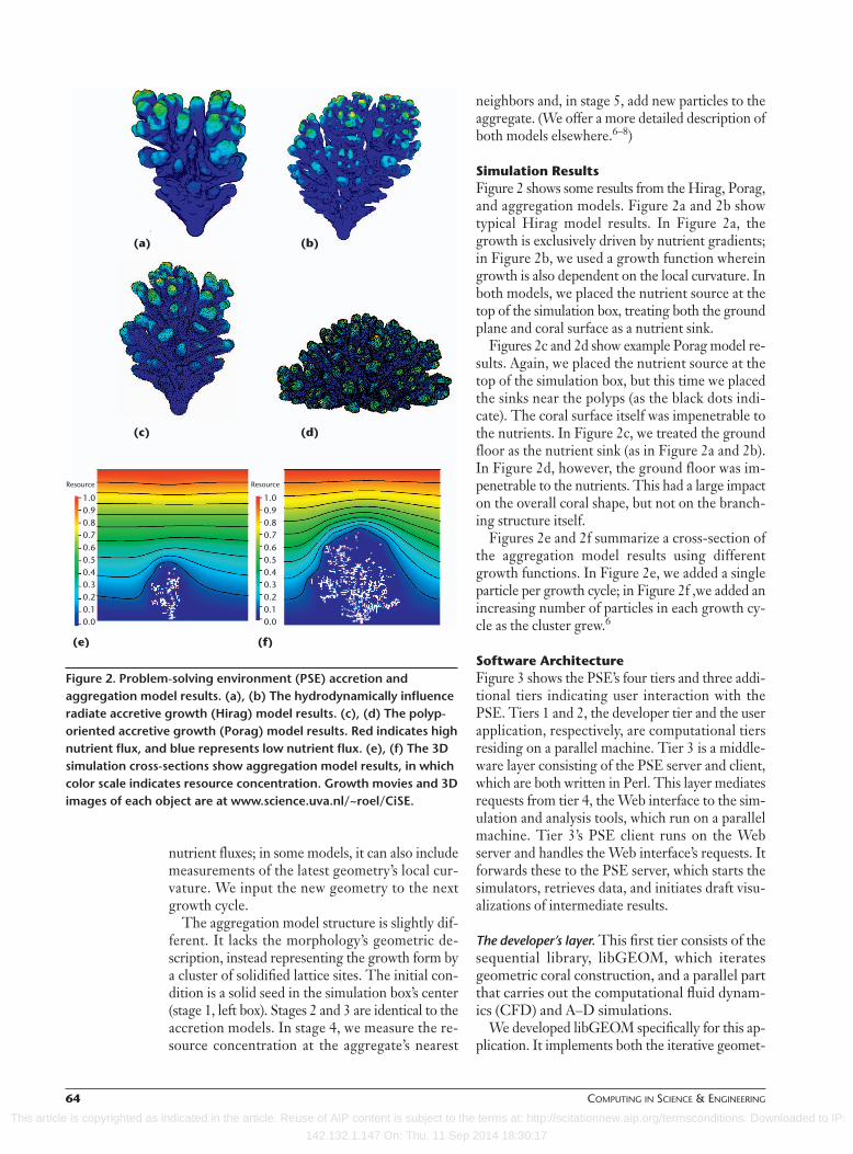
Simulation Results Figure 2 shows some results from the Hirag, Porag,and aggregation models. Figure 2a and 2b showtypical Hirag model results. In Figure 2a, thegrowth is exclusively driven by nutrient gradients;in Figure 2b, we used a growth function whereingrowth is also dependent on the local curvature. Inboth models, we placed the nutrient source at thetop of the simulation box, treating both the groundplane and coral surface as a nutrient sink.

Figures 2c and 2d show example Porag model re-sults. Again, we placed the nutrient source at thetop of the simulation box, but this time we placedthe sinks near the polyps (as the black dots indi-cate). The coral surface itself was impenetrable tothe nutrients. In Figure 2c, we treated the groundfloor as the nutrient sink (as in Figure 2a and 2b).In Figure 2d, however, the ground floor was im-penetrable to the nutrients. This had a large impacton the overall coral shape, but not on the branch-ing structure itself.

Figures 2e and 2f summarize a cross-section ofthe aggregation model results using differentgrowth functions. In Figure 2e, we added a singleparticle per growth cycle; in Figure 2f ,we added anincreasing number of particles in each growth cy-cle as the cluster grew.6

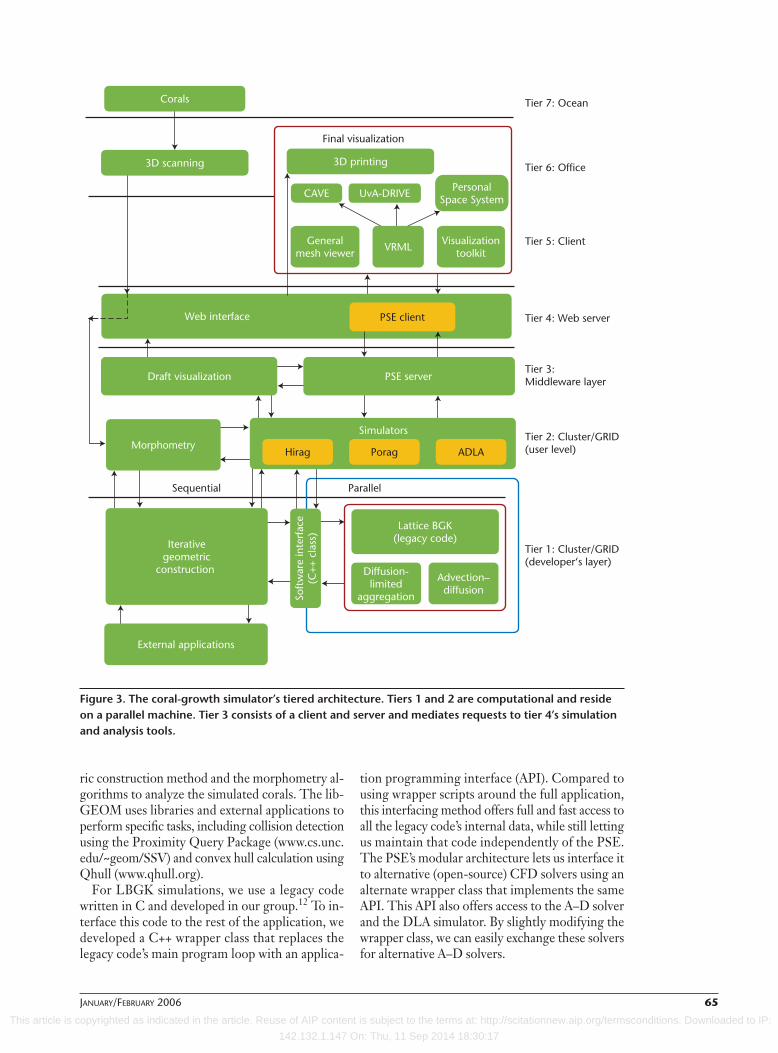
Software ArchitectureFigure 3 shows the PSE’s four tiers and three addi-tional tiers indicating user interaction with thePSE. Tiers 1 and 2, the developer tier and the userapplication, respectively, are computational tiersresiding on a parallel machine. Tier 3 is a middle-ware layer consisting of the PSE server and client,which are both written in Perl. This layer mediatesrequests from tier 4, the Web interface to the sim-ulation and analysis tools, which run on a parallelmachine. Tier 3’s PSE client runs on the Webserver and handles the Web interface’s requests. Itforwards these to the PSE server, which starts thesimulators, retrieves data, and initiates draft visu-alizations of intermediate results.

The developer’s layer. This first tier consists of thesequential library, libGEOM, which iteratesgeometric coral construction, and a parallel partthat carries out the computational fluid dynam-ics (CFD) and A–D simulations.

We developed libGEOM specifically for this ap-plication. It implements both the iterative geomet-

(a) (b)

(c) (d)

(e) (f)

Resource Resource

1.00.9 0.8 0.7 0.6 0.5 0.4 0.3 0.2 0.1 0.0

1.00.9 0.8 0.7 0.6 0.5 0.4 0.3 0.2 0.1 0.0

Figure 2. Problem-solving environment (PSE) accretion andaggregation model results. (a), (b) The hydrodynamically influenceradiate accretive growth (Hirag) model results. (c), (d) The polyp-oriented accretive growth (Porag) model results. Red indicates highnutrient flux, and blue represents low nutrient flux. (e), (f) The 3Dsimulation cross-sections show aggregation model results, in whichcolor scale indicates resource concentration. Growth movies and 3Dimages of each object are at www.science.uva.nl/~roel/CiSE.


142.132.1.147 On: Thu, 11 Sep 2014 18:30:17


ric construction method and the morphometry al-gorithms to analyze the simulated corals. The lib-GEOM uses libraries and external applications toperform specific tasks, including collision detectionusing the Proximity Query Package (www.cs.unc.edu/~geom/SSV) and convex hull calculation usingQhull (www.qhull.org).

For LBGK simulations, we use a legacy codewritten in C and developed in our group.12 To in-terface this code to the rest of the application, wedeveloped a C++ wrapper class that replaces thelegacy code’s main program loop with an applica-

tion programming interface (API). Compared tousing wrapper scripts around the full application,this interfacing method offers full and fast access toall the legacy code’s internal data, while still lettingus maintain that code independently of the PSE.The PSE’s modular architecture lets us interface itto alternative (open-source) CFD solvers using analternate wrapper class that implements the sameAPI. This API also offers access to the A–D solverand the DLA simulator. By slightly modifying thewrapper class, we can easily exchange these solversfor alternative A–D solvers.

Diffusion-limited

aggregation

Advection–diffusion

Lattice BGK(legacy code)

3D scanning

PersonalSpace System

3D printing

Generalmesh viewer

Tier 1: Cluster/GRID(developer‘s layer)

Tier 2: Cluster/GRID(user level)

Tier 6: Office

Tier 5: Client

Tier 3:Middleware layer

Tier 4: Web server

Tier 7: Ocean

Visualizationtoolkit

External applications

Parallel

Web interface

Final visualization

Sequential

CAVE UvA-DRIVE

VRML

Iterativegeometric

construction

Corals

PSE server

Morphometry

Soft

war

e in

terf

ace

(C++

cla

ss)

Simulators

Draft visualization

PSE client

Hirag Porag ADLA

Figure 3. The coral-growth simulator’s tiered architecture. Tiers 1 and 2 are computational and resideon a parallel machine. Tier 3 consists of a client and server and mediates requests to tier 4’s simulationand analysis tools.


142.132.1.147 On: Thu, 11 Sep 2014 18:30:17


Simulation setup. Users interact with the PSEthrough a Web interface (tier 4) that interactswith the user application (tier 2) using the PSEserver (tier 3). The user first specifies the para-meters and initial conditions, and then starts thesimulation, after which the system transparentlysubmits a batch job to the cluster. The Web in-terface enables interaction with the three appli-cation variants—the Hirag, Porag, andaggregation DLA models.

To increase flexibility on the boundary condi-tions, growth function, and growth method (ac-cretion or aggregation), the user can change theuser application’s simulation setup. To accomplishthis, we developed C++ classes that reflect high-

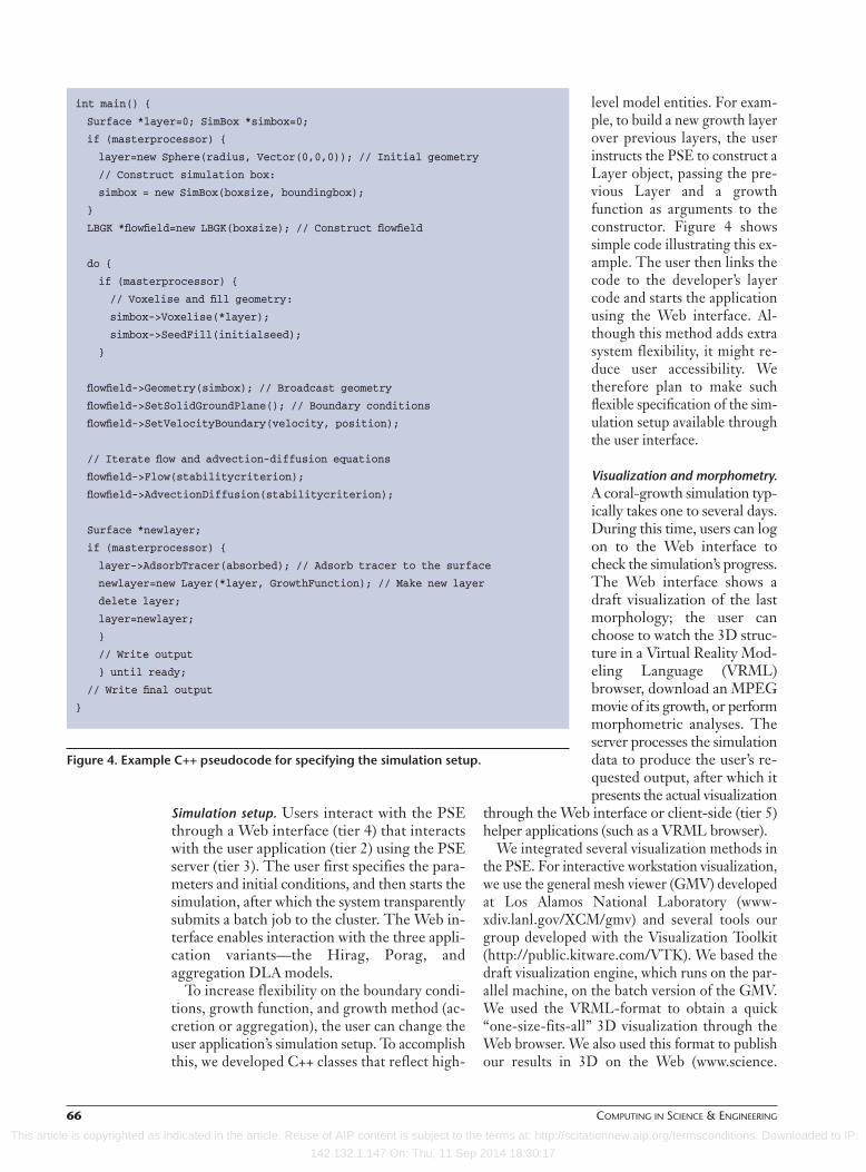
level model entities. For exam-ple, to build a new growth layerover previous layers, the userinstructs the PSE to construct aLayer object, passing the pre-vious Layer and a growthfunction as arguments to theconstructor. Figure 4 showssimple code illustrating this ex-ample. The user then links thecode to the developer’s layercode and starts the applicationusing the Web interface. Al-though this method adds extrasystem flexibility, it might re-duce user accessibility. Wetherefore plan to make suchflexible specification of the sim-ulation setup available throughthe user interface.

Visualization and morphometry.A coral-growth simulation typ-ically takes one to several days.During this time, users can logon to the Web interface tocheck the simulation’s progress.The Web interface shows adraft visualization of the lastmorphology; the user canchoose to watch the 3D struc-ture in a Virtual Reality Mod-eling Language (VRML)browser, download an MPEGmovie of its growth, or performmorphometric analyses. Theserver processes the simulationdata to produce the user’s re-quested output, after which itpresents the actual visualization

through the Web interface or client-side (tier 5)helper applications (such as a VRML browser).

We integrated several visualization methods inthe PSE. For interactive workstation visualization,we use the general mesh viewer (GMV) developedat Los Alamos National Laboratory (www-xdiv.lanl.gov/XCM/gmv) and several tools ourgroup developed with the Visualization Toolkit(http://public.kitware.com/VTK). We based thedraft visualization engine, which runs on the par-allel machine, on the batch version of the GMV.We used the VRML-format to obtain a quick“one-size-fits-all” 3D visualization through theWeb browser. We also used this format to publishour results in 3D on the Web (www.science.

int main() {

Surface *layer=0; SimBox *simbox=0;

if (masterprocessor) {

layer=new Sphere(radius, Vector(0,0,0)); // Initial geometry

// Construct simulation box:

simbox = new SimBox(boxsize, boundingbox);

}

LBGK *flowfield=new LBGK(boxsize); // Construct flowfield

do {


// Voxelise and fill geometry:

simbox->Voxelise(*layer);

simbox->SeedFill(initialseed);

}

flowfield->Geometry(simbox); // Broadcast geometry

flowfield->SetSolidGroundPlane(); // Boundary conditions

flowfield->SetVelocityBoundary(velocity, position);

// Iterate flow and advection-diffusion equations

flowfield->Flow(stabilitycriterion);

flowfield->AdvectionDiffusion(stabilitycriterion);

Surface *newlayer;


layer->AdsorbTracer(absorbed); // Adsorb tracer to the surface

newlayer=new Layer(*layer, GrowthFunction); // Make new layer

delete layer;

layer=newlayer;

}

// Write output

} until ready;

// Write final output

}

Figure 4. Example C++ pseudocode for specifying the simulation setup.


142.132.1.147 On: Thu, 11 Sep 2014 18:30:17


uva.nl/~roel/CiSE) and to display them in immer-sive visualization systems, such as the UvA-DRIVE(www.science.uva.nl/~robbel/DRIVE), the Per-sonal Space System (www.cwi.nl/ins3/), and theCAVE (www.evl.uic.edu/pape/CAVE).

As Figure 5 shows, we’ve also used 3D printingtechniques to demonstrate our results. We con-structed two Porag-model morphologies using se-lective laser sintering. SLS repeatedly applieshorizontal layers of tiny plastic spheres over aslowly lowering plateau; a laser beam melts the par-ticles together and to the previous layers. Such 3Dprints make it possible to visually compare simu-lated morphologies to real morphologies in theuser’s office (tier 6).

For more extensive comparisons between realand simulated morphologies, we scanned severalcorals using a medical computerized tomography(CT) scanner.6 We converted these morphologiesto a triangulated format readable by libGEOM.This let us use the same tools to visualize the sim-ulated and real objects to make a fair visualcomparison—a “Turing test” for morphogenesismodels (www.science.uva.nl/~roel/CDROM/CD/turing.htm). The coral scans also let us analyzereal and simulated coral using the same morpho-metric tools.13

Modeling Multicellular Development EvolutionIn a way, multicellular organisms—including plantsand animals—are enormous cell colonies. As incorals, multicellular organism development emer-ges from the interplay of millions of more or lessindependent modules (cells) whose activities arecoordinated by genetic information and a contin-uous cellular signal exchange.

Biologists often simply speak of “genes” whendiscussing whole organism traits (such as fur color)or more complex traits (such as behavior or mor-phology). They do so knowing, however, that ge-netic information can only directly determine theindividual cell’s behavior, its biophysical properties,and its response to other cells’ signals. To affecttraits of the whole animal or plant, genetic infor-mation must flow, during embryonic development,through a cascade of interactions between ever-larger modules, such as tissues and organs.

Attempting to reconstruct biological multicellu-lar organisms’ evolution would be, of course, tooambitious. Instead, we have evolutionary algo-rithms work on toy models of multicellular crea-tures. In so doing, we get a feeling for evolution’sway of playing—or tinkering—with biologicalbuilding blocks, including cells and genes.

Toy OrganismsThe PSE for multicellular development evolutiondemands differ from those of the coral-growth sys-tem. Simulating a single coral specimen takes along time—typically one to a few days on 16processors. Hence, the coral-growth PSE is mainlytargeted at simulation setup and data postprocess-ing of single runs. In contrast, the simple multicel-lular development model rapidly develops a singlespecimen (within a few minutes on a single proces-sor), but the software must evaluate and comparethousands of individual runs for a meaningful evo-lutionary simulation.

By simulating the evolution of very simple,multicellular creatures—which we call crit-ters14,15—our simulation environment offers us abetter theoretical understanding of

• how genetic information can direct multicellularanimals’ embryonic development; and

• how evolution can mold the genetic informationand “invent” novel development mechanisms.

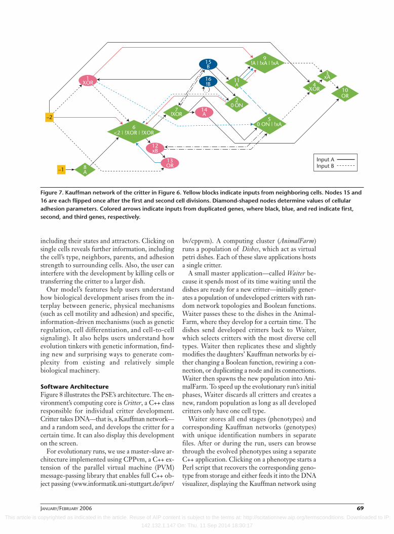
Figure 6 shows a single multicellular critter,which consists of one to a few hundred simulatedcells. These motile cells continuously form andbreak adhesive connections to surrounding cells,favoring stronger over weaker adhesivities. Thisdrives the cells to sort out and end up next to cellsto which they adhere best. Simple, discrete modelsof the genetic regulatory network, as introduced byStuart Kauffman in 1969,16 determine adhesivities(see Figure 7, p. 69). Kauffman networks consist ofseveral genes that can either be in the expressed(“on”) or repressed (“off”) state. Analogous to real

Figure 5. 3D prints generated with selective laser sintering.(Photograph courtesy of Ronald van Weeren.)


142.132.1.147 On: Thu, 11 Sep 2014 18:30:17


cells, in which a gene product (that is, a protein)might bind to another gene’s promoter to activateor inactivate it, the genes in Kauffman networksconnect to other genes, regulating their activity ac-cording to a Boolean function. The network pro-ceeds in discrete time steps, and stabilizes into anattractor, either a fixed state or a cycle, dependingon how the genes are connected and the initial ac-tivation pattern.

In real cells, genetic activity patterns determineentirely whether a cell is, for example, a neuron, astem cell, or a muscle cell. The genetic regulatorynetwork—that is, the network topology and the reg-ulatory gene interaction types (activating, repressive,permissive, and so on)—are entirely determined byDNA, which is identical in each cell of the organism.We follow Kauffman’s suggestion that the network’sattractors can be likened to cell types, and view thenetwork’s topology and Boolean functions as thecritter’s DNA. To account for cell-to-cell commu-nication, the genes can also take inputs from genesin neighboring cells. As with experimental observa-tion in mammalian cells, the cell volume slowly in-creases under mechanical stretch, whereas theyshrink and eventually die if compressed. Thisenables the development of a wide range ofmorphologies and developmental mechanisms rem-iniscent of biological development.14

Development and EvolutionStudying how the critters develop and how that de-velopment evolves will help us gain further insightinto the real biological process. We initiate the sim-ulation with a large cell—the “fertilized egg”—anda randomly connected gene interaction network.

The egg will assume a round shape and have a sta-ble or cyclic cell type. After numerous updates ofthe cell and its genetic network, we divide the cell.Analogous with the gene product gradients thatmany animal species’ mothers deposit in the egg,we flip the state of one of the genes in one of thecells. Most often, this gene flip doesn’t affect thecell state at all, and the critter will develop into anamorphous clump of cells. However, some Kauff-man networks can pick up the maternal informa-tion and produce a second cell type, and additionalmechanisms might produce further cell types.Some critters show developmental mechanismssurprisingly reminiscent of multicellular animalmechanisms.

To find Kauffman networks that can drive thesedevelopmental mechanisms, we use an evolution-ary algorithm that selects for critters with manycell types. We replicate the selected critters, applya small mutation to their Kauffman networks, andlet the new generation develop. Although select-ing for cell type number seems biologically mean-ingless, interesting developmental mechanismsoccur as a side effect of cell differentiation.14,15

Once sufficient critters have evolved, users searchthrough the phenotype storage—the “fossilrecord” of developed critters that appeared in therun—and select interesting critters for furtherstudy. When users click on the image, the systemrecovers the critter’s Kauffman network and feedsit into the Showbeast application. Showbeast is astand-alone application consisting of the PSE’scomputational core and a user interface. Show-beast reruns the developmental process, lettingusers examine the Kauffman networks’ dynamics,

Figure 6. Development of a critter. Colors uniquely identify cell types—that is, Kauffman network attractors. (A movie isavailable at www.science.uva.nl/~roel/CiSE.)


142.132.1.147 On: Thu, 11 Sep 2014 18:30:17


including their states and attractors. Clicking onsingle cells reveals further information, includingthe cell’s type, neighbors, parents, and adhesionstrength to surrounding cells. Also, the user caninterfere with the development by killing cells ortransferring the critter to a larger dish.

Our model’s features help users understandhow biological development arises from the in-terplay between generic, physical mechanisms(such as cell motility and adhesion) and specific,information-driven mechanisms (such as geneticregulation, cell differentiation, and cell-to-cellsignaling). It also helps users understand howevolution tinkers with genetic information, find-ing new and surprising ways to generate com-plexity from existing and relatively simplebiological machinery.

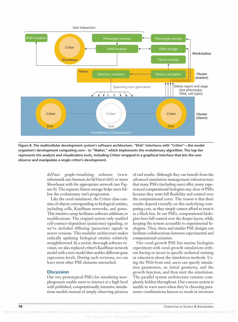
Software ArchitectureFigure 8 illustrates the PSE’s architecture. The en-vironment’s computing core is Critter, a C++ classresponsible for individual critter development.Critter takes DNA—that is, a Kauffman network—and a random seed, and develops the critter for acertain time. It can also display this developmenton the screen.

For evolutionary runs, we use a master–slave ar-chitecture implemented using CPPvm, a C++ ex-tension of the parallel virtual machine (PVM)message-passing library that enables full C++ ob-ject passing (www.informatik.uni-stuttgart.de/ipvr/

bv/cppvm). A computing cluster (AnimalFarm)runs a population of Dishes, which act as virtualpetri dishes. Each of these slave applications hostsa single critter.

A small master application—called Waiter be-cause it spends most of its time waiting until thedishes are ready for a new critter—initially gener-ates a population of undeveloped critters with ran-dom network topologies and Boolean functions.Waiter passes these to the dishes in the Animal-Farm, where they develop for a certain time. Thedishes send developed critters back to Waiter,which selects critters with the most diverse celltypes. Waiter then replicates these and slightlymodifies the daughters’ Kauffman networks by ei-ther changing a Boolean function, rewiring a con-nection, or duplicating a node and its connections.Waiter then spawns the new population into Ani-malFarm. To speed up the evolutionary run’s initialphases, Waiter discards all critters and creates anew, random population as long as all developedcritters only have one cell type.

Waiter stores all end stages (phenotypes) andcorresponding Kauffman networks (genotypes)with unique identification numbers in separatefiles. After or during the run, users can browsethrough the evolved phenotypes using a separateC++ application. Clicking on a phenotype starts aPerl script that recovers the corresponding geno-type from storage and either feeds it into the DNAvisualizer, displaying the Kauffman network using

–2 50 ON | !xA6

<2 | !XOR | !XOR

11A

12xB

13OR

3xA

10OR

!A | !xA | !xA

4XOR

15B

9

–1 8A

14A

7!XOR

20 ON

Input AInput B

1XOR !B

16

Figure 7. Kauffman network of the critter in Figure 6. Yellow blocks indicate inputs from neighboring cells. Nodes 15 and16 are each flipped once after the first and second cell divisions. Diamond-shaped nodes determine values of cellularadhesion parameters. Colored arrows indicate inputs from duplicated genes, where black, blue, and red indicate first,second, and third genes, respectively.


142.132.1.147 On: Thu, 11 Sep 2014 18:30:17


daVinci graph-visualizing software (www.informatik.uni-bremen.de/daVinci/old/) or startsShowbeast with the appropriate network (see Fig-ure 8). The separate fitness storage helps users fol-low the evolutionary run’s progression.

Like the coral simulators, the Critter class con-sists of objects corresponding to biological entities,including cells, Kauffman networks, and genes.This intuitive setup facilitates software additions ormodifications. The original system only enabledcell-contact-dependent (juxtacrine) signaling, sowe’ve included diffusing (paracrine) signals innewer versions. This modular architecture makesradically updating biological entities relativelystraightforward. In a recent, thorough software re-vision, we also replaced critter’s Kauffman networkmodel with a new model that enables different geneexpression levels. During such revisions, we canleave most other PSE elements untouched.

DiscussionOur two prototypical PSEs for simulating mor-phogenesis enable users to interact at a high levelwith published, computationally intensive simula-tions models instead of simply observing pictures

of end results. Although they can benefit from theadvanced simulation management infrastructurethat many PSEs (including ours) offer, many expe-rienced computational biologists stay clear of PSEsbecause they want full flexibility and control overthe computational cores. The reason is that theirresults depend crucially on this underlying com-puting core, so they simply cannot afford to treat itas a black box. In our PSEs, computational biolo-gists have full control over the deeper layers, whilekeeping the system accessible to experimental bi-ologists. Thus, these and similar PSE designs canfacilitate collaborations between experimental andcomputational scientists.

Our coral-growth PSE lets marine biologistsexperiment with coral-growth simulations with-out having to invest in specific technical trainingor education about the simulation methods. Us-ing the Web front end, users can specify simula-tion parameters, an initial geometry, and thegrowth function, and then start the simulation.The parallel system architecture remains com-pletely hidden throughout. Our current system isunable to warn users when they’re choosing para-meter combinations known to result in incorrect

Critter Critter

Dishes report end stage

DNA, cell types)(last phenotype,

Critter

DNA visualizer

AnimalFarm (16 processors)

Cluster(slaves)

Cluster(master)

Workstation

Spawning new generation

User interaction

Waiter

Phenotype storage

Fitness storage

DNA storageDNA localizer

Phenotype browser

Selection mutation Fitness calculation

Critter

Showbeast

Dish Dish Dish

Figure 8. The multicellular development system’s software architecture. “Dish” interfaces with “Critter”—the modelorganism’s development computing core—to “Waiter,” which implements the evolutionary algorithm. The top tierrepresents the analysis and visualization tools, including Critter wrapped in a graphical interface that lets the userobserve and manipulate a single critter’s development.


142.132.1.147 On: Thu, 11 Sep 2014 18:30:17


results. We’ll include such knowledge in futurePSE versions; for example, we could easily inte-grate knowledge about valid flow velocity and dif-fusion coefficient11 combinations. Our PSE formulticellular development efficiently implementsan evolutionary search for interesting critters ona parallel architecture. It also both facilitates ex-plorations of evolutionary history and individualcritter analysis.

Simulation FlexibilityAlthough PSEs can make some simulation systemsmore manageable and accessible, they might im-pose unacceptable restrictions on others. Wetherefore used tiered and modular architectures.The deeper users proceed into the PSEs’ archi-tectures, the more computational skills they’ll needin return for the increased flexibility. If users aren’tsatisfied with the standard setup, for example, bothPSEs will let them create a new setup with thehigh-level C++ objects. This requires basic knowl-edge of C++ programming, but the deeper li-braries can be safely considered a black box. Whenthe main program structure is kept untouched, thenew simulation setup transparently interfaces tothe Web server.

Users with more technical knowledge can easilyreplace simulation elements with alternatives. Inthe coral-growth simulations, for example, themodular architecture lets users swap the CFD andA–D solvers for different solvers. We’re now col-laborating with the national research institute formathematics and computer science (CWI) inAmsterdam to do precisely that, since we’re cur-rently hitting these solvers’ limits. (The currentA–D method produces incorrect results when ad-vective transport becomes much more importantthan diffusive transport.11)

The Best of Both WorldsMorphogenesis simulations are often not onlyhigh-performance applications, but also high-throughput applications. Here, we’ve shownexamples of both: single coral simulation is com-putationally intensive, thus we can only simulate afew; simulating one critter is cheap, but we needmany of them. Ultimately, we want to evaluate nu-merous biologically realistic, computationally moreintensive morphogenesis problems.

For example, to understand each parameter’srole in the coral-growth model, we must performparameter sweeps to construct so-called “mor-phospaces.”17 These theoretical growth-form or-derings can map out the existing and non-existingshapes that the modeled growth mechanism pro-

duces. They’re helpful for analyzing the growthprocess and interpreting existing growth forms’functional advantage. The critter model’s inde-pendent parameters are so numerous that com-pletely mapping the morphospace is infeasibleand insensible, but as our research shows, evolu-tionary computation can nevertheless give us in-sights into the general properties of thisenormous search space.

Realistic morphogenesis simulations are compu-tationally very expensive (a typical Porag modelsimulation requires 18 to 36 hours on 16 Beowulfprocessors). Given this, such extensive parametersweeps aren’t yet feasible. Moreover, conventionalhigh-throughput architectures such as Condor(www.cs.wisc.edu/condor) are often unsuitable formanaging high-performance applications. Moresuitable architectures for dynamically managinghigh-performance applications include grid-en-abled Dynamite (now in development; see www.science.uva.nl/research/scs/Software/index.html)and grid-enabled parameter-sweep architecturessuch as Nimrod/G (www.csse.monash.edu.au/~davida/nimrod/nimrodg.htm). In future work, weplan to interface our morphogenesis PSEs to acombination of Dynamite and Nimrod/G toefficiently execute high-throughput, high-performance morphogenesis simulations on com-putational grids.

Computational modeling is becomingan ever more essential tool in biologi-cal research. Recent advances inexperimental biology, including large-

scale functional genomic screens that systemati-cally map out how knocking out or overexpressinggenes affect the organism’s appearance, growth,and behavior, call for methods that help unravelhow (that is, through which mechanisms) a generegulates the organism. Such “how” questions re-quire insight into the physical and biological in-teractions of thousands of cells (whose behaviormight be affected by a genetic mutation), whichresult in the (possibly abnormal) growth and formof the organism.

Our long-term goal is to bring simulation toolsto the experimentalist’s lab bench, which alreadycontains bioinformatics and image analysis tools.To reach that goal, the experimentalist must beable to easily tinker with the underlying model,without compromising the computational biolo-gist’s ability to work on the underlying com-putational core. New PSE designs combiningextensible domain-specific languages with the sim-


142.132.1.147 On: Thu, 11 Sep 2014 18:30:17


ulation management systems we’ve described here,along with intensive collaborations between ex-perimental and computational biologists, mightbring that goal a little closer.

AcknowledgmentsWe thank Robert van Liere (CWI, Amsterdam) forvisualizing our simulation results on the Personal SpaceStation; Robert Belleman (UvA) for the UvA-DRIVE andCAVE system visualizations; Leo E.H. Lampmann (St.Elisabeth Ziekenhuis, Tilburg) for making 3D scans ofcoral skeletons, kindly made available by Mark Vermeij(Cooperative Institute for Marine and AtmosphericStudies, Miami), and Rolf Bak (Netherlands Institute forSea Research and UvA). We also thank Ronald vanWeeren (Artis Zoo, Amsterdam) for photography of theSLS-prints of the coral models, and Zeger Hendrikse(UvA) and Kamil Iskra (UvA) for fruitful discussions.

References1. J.R. Rice and R.F. Boisvert, “From Scientific Software Libraries to

Problem-Solving Environments,” IEEE Computational Science andEng., vol. 3, no. 3, 1996, pp. 44–53.

2. L.A. Segel, “Computing an Organism,” Proc. Nat’l Academy ofSciences, vol. 98, no. 7, 2001, pp. 3639–3640.

3. A.F.M. Marée and P. Hogeweg, “How Amoeboids Self-Organizeinto a Fruiting Body: Multicellular Coordination in DictyosteliumDiscoideum,” Proc. Nat’l Academy of Sciences, vol. 98, no. 7,2001, pp. 3879–3883.

4. R.M.H. Merks and J.A. Glazier, “A Cell-Centered Approach to De-velopmental Biology,” Physical Rev. A, vol. 352, no. 1, 2005, pp.113–130.

5. T. Cickovski et al., “A Framework for Three-Dimensional Simula-tion of Morphogenesis,” IEEE/ACM Trans. Computational Biologyand Bioinformatics, vol. 2, no. 3, 2005, pp. 1–16.

6. J. Kaandorp and J. Kübler, eds., The Algorithmic Beauty of Sea-weeds, Sponges, and Corals, Springer-Verlag, 2001.

7. R.M.H. Merks et al., “Models of Coral Growth: SpontaneousBranching, Compactification and the Laplacian Growth As-sumption,” J. Theoretical Biology, vol. 224, no. 2, 2003, pp.153–166.

8. R.M.H. Merks et al., “Polyp Oriented Modelling of CoralGrowth,” J. Theoretical Biology, vol. 228, no. 4, 2004, pp.559–576.

9. T. Witten and L. Sander, “Diffusion-Limited Aggregation, A Ki-netic Critical Phenomenon,” Physical Rev. Letters, vol. 47, no. 19,1981, pp. 1400–1403.

10. S. Succi et al., “Applying the Lattice Boltzmann Equation to Mul-tiscale Fluid Problems,” Computing in Science & Eng., vol. 3, no.6, 2001, pp. 26–37.

11. R.M.H. Merks, A.G. Hoekstra, and P.M.A. Sloot, “The MomentPropagation Method for Advection-Diffusion in the Lattice Boltz-mann Method: Validation and Péclet Number Limits,” J. Com-putational Physics, vol. 183, no. 2, 2002, pp. 563–576.

12. D. Kandhai et al., “Implementation Aspects of 3D Lattice-BGK:Boundaries Accuracy and a New Fast Relaxation Method,” J.Computational Physics, vol. 150, no. 2, 1999, pp. 482–501.

13. J.A. Kaandorp et al., “Morphogenesis of the Branching Reef CoralMadracis Mirabilis,” Proc. Royal Soc. London B, vol. 272, no. 1559,2005, pp. 127–133.

14. P. Hogeweg, “Evolving Mechanisms of Morphogenesis: On theInterplay between Differential Adhesion and Cell Differentiation,”

J. Theoretical Biology, vol. 203, no. 4, 2000, pp. 317–333.

15. P. Hogeweg, “Computing an Organism: On the Interface be-tween Informatic and Dynamic Processes,” Biosystems, vol. 64,nos. 1–3, 2002, pp. 97–109.

16 S.A. Kauffman, “Metabolic Stability and Epigenesis in RandomlyConnected Nets,” J. Theoretical Biology, vol. 22, no. 3, 1969, pp.437–467.

17. G.R. McGhee, Theoretical Morphology: The Concept and Its Appli-cations, Colombia Univ. Press, 1999.

Roeland M.H. Merks is a postdoc in the plant systems bi-ology department at the Flanders Interuniversity Institutefor Biotechnology in Ghent, Belgium, where he works withexperimental biologists to model leaf morphogenesis. Hismain research interest is in biological morphogenesismodeling, including coral growth, vascular developmentin mammals and plants, and leaf growth. Merks has aPhD in computational science from the University of Am-sterdam. Contact him at [email protected]; www.roelandmerks.nl.

Alfons G. Hoekstra is an associate professor at the Uni-versity of Amsterdam, where his research interests includescientific grid computing and Lattice-Boltzmann model-ing and simulation. Hoekstra has a PhD in computationalscience from the University of Amsterdam. Contact him [email protected].

Jaap A. Kaandorp is an assistant professor in the com-putational science section of the Faculty of Science at theUniversity of Amsterdam. His research interests are in mor-phogenesis, marine sessile organisms, evolutionaryprocesses, modeling and simulation of developmental reg-ulatory networks and metabolic pathways, modeling andsimulation of growth and form, and biomechanics. Kaan-dorp has a PhD in computer science and mathematicsfrom the University of Amsterdam. Contact him at [email protected].

Peter M.A. Sloot is a professor of computer simulation atthe University of Amsterdam, where he heads the Com-puting, System Architecture, and Programming Labora-tory. His research interest is in information processing incomplex dynamical systems and distributed simulationenvironments. Contact him at [email protected]; www.science.uva.nl/research/scs.

Paulien Hogeweg is a professor of theoretical biology andbioinformatics at Utrecht University. Her research inter-ests include prebiotic evolution, genome evolution, mor-phogenesis, eco-evolutionary dynamics, and the interplaybetween evolution and learning. In the 1970s, she coinedthe term “bioinformatics” for the study of informaticprocesses in biotic systems. Contact her at [email protected]; http://bioinformatics.bio.uu.nl.


142.132.1.147 On: Thu, 11 Sep 2014 18:30:17

Documents

Problem-solving environments for biological morphogenesis