PROBING THE MECHANICAL PROPERTIES OF SHORT

MOLECULES WITH OPTICAL TWEEZERS

by

Benjamin P. B. Downing B. Sc. (Honours), Dalhousie University, 2007

THESIS SUBMITTED IN PARTIAL FULFILLMENT OF THE REQUIREMENTS FOR THE DEGREE OF

MASTER OF SCIENCE

In the Department of Physics

© Benjamin P. B. Downing 2010

SIMON FRASER UNIVERSITY

Spring 2010

All rights reserved. However, in accordance with the Copyright Act of Canada, this work may be reproduced, without authorization, under the conditions for Fair Dealing. Therefore, limited reproduction of

this work for the purposes of private study, research, criticism, review and news reporting is likely to be in accordance with the law,

particularly if cited appropriately.

ii

APPROVAL

Name: Benjamin P. B. Downing

Degree: Master of Science

Title of Thesis: Probing the mechanical properties of short molecules with optical tweezers

Examining Committee:

Chair: Dr. Michel C. Vetterli Professor of Physics

___________________________________________

Dr. Nancy R. Forde Senior Supervisor Assistant Professor of Physics

___________________________________________

Dr. Eldon Emberly Supervisor Associate Professor of Physics

___________________________________________

Dr. John Bechhoefer Supervisor Professor of Physics

___________________________________________

Dr. Edgar C. Young Internal Examiner Assistant Professor of Molecular Biology and Biochemistry

Date Defended: March 11th, 2010

Last revision: Spring 09

Declaration ofPartial Copyright Licence

The author, whose copyright is declared on the title page of this work, has granted to Simon Fraser University the right to lend this thesis, project or extended essay to users of the Simon Fraser University Library, and to make partial or single copies only for such users or in response to a request from the library of any other university, or other educational institution, on its own behalf or for one of its users.

The author has further granted permission to Simon Fraser University to keep or make a digital copy for use in its circulating collection (currently available to the public at the “Institutional Repository” link of the SFU Library website <www.lib.sfu.ca> at: <http://ir.lib.sfu.ca/handle/1892/112>) and, without changing the content, to translate the thesis/project or extended essays, if technically possible, to any medium or format for the purpose of preservation of the digital work.

The author has further agreed that permission for multiple copying of this work for scholarly purposes may be granted by either the author or the Dean of Graduate Studies.

It is understood that copying or publication of this work for financial gain shall not be allowed without the author’s written permission.

Permission for public performance, or limited permission for private scholarly use, of any multimedia materials forming part of this work, may have been granted by the author. This information may be found on the separately catalogued multimedia material and in the signed Partial Copyright Licence.

While licensing SFU to permit the above uses, the author retains copyright in the thesis, project or extended essays, including the right to change the work for subsequent purposes, including editing and publishing the work in whole or in part, and licensing other parties, as the author may desire.

The original Partial Copyright Licence attesting to these terms, and signed by this author, may be found in the original bound copy of this work, retained in the Simon Fraser University Archive.

Simon Fraser University LibraryBurnaby, BC, Canada

iii

ABSTRACT

Structural proteins play vital roles in many human tissues, roles to which their mechanical properties are of direct relevance. Optical tweezers give us the remarkable ability to quantitatively probe these properties at the single-molecule level, potentially revealing a wealth of information on how such proteins fulfil their physiological functions. I have worked toward applying this technique, in which micron-sized beads chemically linked to the protein are manipulated by focussed laser beams, to structural proteins, particularly elastin. I developed methods to eliminate or account for several experimental complications presented by the fact that these proteins are short compared to other molecules studied with optical tweezers. I proceeded to design and test multiple strategies for linking elastin to beads, discovering that its unusual biochemical properties raise significant additional challenges. Some of these I overcame, and an assay I developed for linking effectiveness may be of use in overcoming others.

Keywords: optical tweezers; single-molecule force spectroscopy; short molecules; elastin; structural proteins

iv

DEDICATION

To Nan and Grandpa.

v

ACKNOWLEDGEMENTS

A great number of people have helped me with this thesis, and supported me while I worked on it. I would like to take this opportunity to thank them.

I want to begin by thanking the members of the Forde lab, past and present, a group that I feel very lucky to have been a part of. Though many people have come and gone during my time in the lab, it has always remained a group that is a pleasure both to work with and to relax with. I owe an extra thank you to Andrew, for sharing his “decades of experience” in the biochemical arts with me, to Yi, for passing his optical tweezers on to me, and to Rob for all his hard work on the elastin project. I also want to thank Nancy for leading such a great group, and for genuinely caring, not only about the research, but also about her students.

I have had the good fortune to collaborate with Fred and Megan at the University for Sick Children in Toronto, and I thank them for their explanations of elastin’s mysteries of a physicist, their good humour and enthusiasm, and for giving me elastin to play with.

I thank my friends and family, for always being there to support me when I needed it. Finally, I want to thank Helen, my mom, for everything, but especially for helping me discover how to learn for myself.

vi

TABLE OF CONTENTS

Approval ............................................................................................................................ ii

Abstract............................................................................................................................. iii

Dedication ......................................................................................................................... iv

Acknowledgements ........................................................................................................... v

Table of Contents ............................................................................................................. vi

List of Figures................................................................................................................. viii

List of Tables .................................................................................................................. xiii

1 Introduction .................................................................................................. 1 1.1 Forces in biological systems........................................................................... 1 1.2 Force-extension curves ................................................................................... 4 1.3 Elastin ............................................................................................................. 7

1.3.1 The properties and physiological role of elastin......................................... 7 1.3.2 Relevance of single-molecule mechanical studies to elastin.................... 10

2 Optical Tweezers......................................................................................... 12 2.1 Principles of optical trapping........................................................................ 12 2.2 The optical tweezers instrument ...................................................................15

2.2.1 Laser and optical set up ............................................................................ 15 2.2.2 Bead manipulation .................................................................................... 17 2.2.3 Sample delivery system ............................................................................ 19 2.2.4 Measurement and calibration.................................................................... 22

3 The Effects of Short Separations on Optical Tweezers Measurements ............................................................................................. 27

3.1.1 Optical interactions................................................................................... 28 3.1.2 Static forces .............................................................................................. 31 3.1.3 Hydrodynamics......................................................................................... 33 3.1.4 Excluded volume ...................................................................................... 39 3.1.5 Summary of short separation results......................................................... 41

4 Applying Optical Tweezers to Elastin ...................................................... 42 4.1 Linking strategies ......................................................................................... 42

4.1.1 Biotin/streptavidin .................................................................................... 43 4.1.2 Fluorescein/anti-fluorescein ..................................................................... 44 4.1.3 Covalent crosslinking ............................................................................... 44

4.2 Specific challenges tethering elastin.............................................................44

vii

4.2.1 Elastin-induced bead flocculation............................................................. 45 4.2.2 Variability of force-extension curves ....................................................... 46 4.2.3 Testing tethering strategies ....................................................................... 54

4.3 Summary of work with elastin ..................................................................... 60

5 Conclusions and Outlook ........................................................................... 62 5.1 Conclusions .................................................................................................. 62 5.2 Future work .................................................................................................. 63

Appendix A: Linking Protocols ..................................................................................... 66 A.1 Crosslinking streptavidin to beads using EDC............................................. 66 A.2 Linking fluorescein to protein G beads using DMP..................................... 67 A.3 Crosslinking elastin to beads using ECMA.................................................. 68 A.4 Crosslinking elastin to beads via Sulfo-SMCC............................................ 70

Appendix B: Linking Assay ........................................................................................... 72 B.1 Protocol for linking assay............................................................................. 72

References ........................................................................................................................ 74

viii

LIST OF FIGURES

Figure 1.1: Diagrams of single-molecule extension measurements using (a) optical tweezers and (b) atomic force microscopy. .......................................... 3

Figure 1.2: Force versus extension plot of a single 11.7 kilobasepair double-stranded DNA molecule (3.95 µm contour length) measured in our optical tweezers instrument using the protocol described in [13]. Open circles: extension of molecule; solid squares: relaxation of the same molecule; line: worm-like-chain fit (equation 1.2) to force-extension data below 5 pN, with fitting parameters L = 3.9 µm and P = 60 nm. ............. 5

Figure 1.3: Diagrams of (a) the freely jointed chain polymer model and (b) the worm-like chain polymer model, including definitions of the Kuhn length, K, and persistence length, P. ................................................................ 6

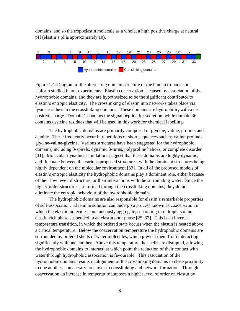
Figure 1.4: Diagram of the alternating domain structure of the human tropoelastin isoform studied in our experiments. Elastin coacervation is caused by association of the hydrophobic domains, and they are hypothesized to be the significant contributor to elastin’s entropic elasticity. The crosslinking of elastin into networks takes place via lysine residues in the crosslinking domains. These domains are hydrophilic, with a net positive charge. Domain 1 contains the signal peptide for secretion, while domain 36 contains cysteine residues that will be used in this work for chemical labelling.............................................................................. 9

Figure 2.1: Optical trapping as described by ray optics. (a) Origin of the gradient force. The sphere is illuminated by a beam with a linear intensity gradient, and two representative rays at symmetric positions about the bead centre are drawn. The momenta changes for the light rays are illustrated to the right, showing that the intensity difference produces a net force on the bead up the intensity gradient. (b) Optical trapping along the optical axis. For a bead centred in the beam all forces perpendicular to the axis cancel, while the net force is directed toward the beam focus. (c) Optical trapping perpendicular to the optical axis. As the bead is displaced from the axis the beam is deflected in the same direction, producing a restoring force on the bead................................ 14

Figure 2.2: Diagram of the optical layout of our optical tweezers instrument. See text for details. ................................................................................................ 16

Figure 2.3: (a) Image of a 1.27 µm diameter polystyrene bead immobilized on a micropipette tip using suction, and a 2.1 µm diameter trapped bead, in

ix

our apparatus. (b) Diagram of a micropipette mounted in a sample chamber. ......................................................................................................... 18

Figure 2.4: (a) Diagram of fluidics delivering buffer and beads to chamber. The valves can be used to shut off buffer flow in the chamber. Valve 1 is also used to switch between buffers containing different microsphere species. (b) to (d): because fluid flow is laminar there is no turbulent mixing of the different buffers. The position of the flow boundary can be modified by changing the relative pressure of the two inputs. In this apparatus pressure is controlled by raising or lowering the input reservoirs. ....................................................................................................... 21

Figure 2.5: Power spectrum of a trapped 2.10 µm diameter microsphere and the corresponding Lorentzian fit, giving fc = 950 Hz. .......................................... 26

Figure 3.1: Diagram showing a possible interaction of the pipette-mounted bead with the trapping laser. Approximately to scale for 2.1 µm diameter beads. .............................................................................................................. 28

Figure 3.2: Photodiode output as a function of pipette-mounted bead position in the laser’s focal plane. The x and y readings are proportional to the deflection of the laser in the x and y directions. Left column displays data for a 2.1 µm diameter bead, right column for a 1.27 µm bead. The blue lines indicate the trajectory of the pipette-mounted bead during a single-molecule stretching experiment, and the end of each line marks the trap centre. Deflection in the y direction along this trajectory is shown in Figure 3.3 (b). ............................................................. 29

Figure 3.3: (a) Diagram of experiment to probe interactions of pipette-mounted bead with laser. (b) Plot of laser deflection as a function of pipette-mounted bead position for a 2.1 µm bead (dotted red line) and a 1.27 µm bead (solid blue line). The data is interpolated along the blue lines shown in Figure 3.2. The vertical dashed line indicates the position of the pipette-mounted bead at which it will make contact with trapped bead, if one bead has a diameter of 2.1 µm and the other 1.27 µm................ 31

Figure 3.4: (a) Diagram of the experiment performed to quantify static forces between beads. (b) Plots of the forces exerted on a trapped bead as a function of the separation between the beads. Open blue circles show data collected in ultra pure water, while solid red squares indicate data collected in a 0.1 M KCl solution. In both cases, both beads were carboxylated polystyrene................................................................................ 32

Figure 3.5: (a) Diagram showing the position of the pipette during the collection of power spectra for the determination of hydrodynamic effects, including a definition of the axes. (b) and (c) power spectra of Brownian motion, in the x and y directions, respectively, of a trapped bead for different separations between the beads........................................... 34

Figure 3.6: (a) Corner frequency, (b) drag coefficient, and (c) trap stiffness calculated from Lorentzian fits to the power spectra of Figure 3.5,

x

plotted as functions of bead separation. Open triangles show data from Brownian motion in the y direction and solid squares show data from Brownian motion in the x direction. Dashed vertical lines indicate the point at which the two beads nominally come into contact. Error bars in (a) and (c) come from fitting uncertainty. Error bars in (b) are not shown, as they are comparable in size to the data points. ............ 35

Figure 3.7: Normalized drag coefficients plotted as a function of normalized bead separation, S. Open triangles and solid squares indicate measured data points for the y and x directions, respectively. Solid black and red lines indicate the theoretical predictions for two beads [52] for y and x directions respectively. Dashed black and red lines indicate the theoretical predictions for a bead approaching an infinite plane [48] for y and x directions respectively. ................................................................. 37

Figure 3.8: (a) Diagram of a free molecule as used in standard FJC and WLC polymer model calculations, in which all molecular configurations are allowed. (b) and (c) diagrams of types of excluded volume which may affect molecular-extension experiments: (b) a molecular configuration disallowed because the polymer is excluded from the bead volume (polymer exclusion), and (c) a molecular configuration disallowed because the free bead is excluded from the volume of the fixed bead (bead exclusion)............................................................................ 40

Figure 4.1: Schematic diagram of elastin tethering strategies. The N-terminus of the protein is labelled with biotin, allowing it to be tethered to streptavidin-coated beads via a ligand/receptor interaction. Three different strategies were designed for linking the C-terminus: two using covalent crosslinkers and one using an antibody-antigen interaction. ...................................................................................................... 43

Figure 4.2: Representative examples of force-extension curves from different tethers. The experiments were conducted with anti-fluorescein-coated polystyrene beads incubated with fluorescein- and biotin-labelled elastin, and streptavidin-coated polystyrene beads. The curves show a wide variety of behaviour. .............................................................................. 47

Figure 4.3: Example of a force-extension curve for multiple DNA tethers, measured in our optical tweezers apparatus using the same protocol as Figure 1.2. Each discontinuity is the result of one of the tethers breaking. ......................................................................................................... 49

Figure 4.4: Left: diagram of an elastin molecule tethered non-specifically between two beads. Right: diagram of elastin molecule specifically linked to one bead and non-specifically bound to another. ........................................... 50

Figure 4.5: Representative force-extension curves collected from pairs of carboxylated polystyrene beads. Solid diamonds indicate curves from uncoated beads at pH 5.0, while open squares indicate curves from pairs of streptavidin and anti-fluorescein coated beads at pH 7.4.

xi

These curves show that the beads interact significantly when brought into contact even when elastin is not present, making it difficult to determine which, if any, of our previously measured curves resulted from extending elastin molecules. .................................................................. 53

Figure 4.6: Native gel testing the biotinylation of elastin. Elastin was modified in three different ways: biotinylated; biotinylated and fluorescein labelled with one potential site; and biotinylated and fluorescein labelled with two potential sites. Samples of each were run both with and without prior incubation with streptavidin. All samples incubated with streptavidin show a reduction of signal in the band corresponding to single molecules (A) and the appearance of a second, more slowly migrating band (B), corresponding to multiple elastin molecules attached together. This indicates a portion of each population has been effectively biotinylated, allowing biotin-streptavidin binding. The percent reductions in free elastin estimated by image analysis are provided in the legend. Experiment conducted and figure provided by Ming Miao. ..................................................................................................... 56

Figure 4.7: Diagram of pNPP assay for the linking of biotinylated molecules to beads. Streptavidin-alkaline-phosphatase binds to the biotin tag and catalyzes the hydrolysis of pNPP producing an absorbent product. The absorbance can be used to determine the quantity of biotinylated tethers. ............................................................................................................ 58

Figure 4.8: Results of pNPP assay for digoxigenin- and biotin-labelled DNA binding to antibody-coated beads. Error bars are standard deviations (N=3). The increase in signal with increasing DNA concentration for anti-fluorescein-coated beads indicates that DNA can bind non-specifically to the beads. The more pronounced increase for anti-digoxigenin coated beads confirms that the digoxigenin-anti-digoxigenin interaction specifically tethers DNA to the beads. The finite signal for beads without DNA shows that streptavidin-alkaline-phosphatase also binds non-specifically to the beads. The beads were incubated with pNPP for a duration of one hour. ........................................... 59

Figure 4.9: Results of the pNPP assay for covalent coupling of elastin to carboxylated silica beads via Sulfo-SMCC. A similar increase in signal with increasing elastin concentration can be seen for samples prepared both with and without the crosslinker, indicating that both are the result of non-specific interactions. This confirms that elastin can bind non-specifically to silica beads and that the covalent coupling protocol was not effective. The finite signal for the sample with no elastin present shows that streptavidin-alkaline-phosphatase can bind non-specifically to silica beads. The beads were incubated with pNPP for only 20 minutes, so a quantitative comparison of the normalized absorbance values in this figure with those in Figure 4.8 is not possible. .......................................................................................................... 60

xii

Figure 5.1: Diagram of linking strategies for pulling on elastin with either one or two DNA handles. .......................................................................................... 64

xiii

LIST OF TABLES

Table 4.1: List of conditions under which tethering of elastin was attempted. F-AF and B-SA refer to the fluorescein-anti-fluorescein and biotin-streptavidin linking strategies, respectively. ECMA and Sulfo-SMCC refer to covalent crosslinkers. .......................................................................... 51

Table 4.2: List of conditions under which control experiments were conducted to test for non-specific interactions of elastin, linking proteins, and beads. ........ 54

1

1 INTRODUCTION

The human body is a complex structure whose ability to support and maintain itself against the constant barrage of forces to which it is exposed depends on the interplay of structural elements across a vast array of scales, ranging from the metre-long vertebral column to sub-nanometre molecular bonds. Fibrillar structural proteins play key roles in the integrity of the body, and show distinct hierarchical organization at almost all of the relevant length-scales. Understanding the relationship between the structure of these proteins, their mechanical properties, their higher level organization, and their roles in making functional tissues is a multifaceted problem, but one which is of relevance to human health and materials engineering, and incorporates much fundamental physics.

In this work, I approached the problem at the molecular level. My goal was to probe the mechanical properties of individual fibrillar structural proteins, particularly elastin, which is responsible for the elastic behaviour of many tissues. My chosen tool was optical tweezers, a powerful technique for applying and measuring forces on the picoNewton scale. The application of this tool to elastin presents significant challenges, some arising from the short contour lengths common to many fibrillar proteins, and others from the unusual biochemistry of elastin. This thesis describes my efforts to overcome these challenges. The remainder of this chapter discusses the relevance of forces to biological systems at the molecular scale and some of the basic tools used to measure and understand them. It also introduces elastin, its physiological role and biochemistry. The second chapter outlines the theory of optical tweezers and describes the optical trapping apparatus I used. The third chapter explains the experimental challenges associated with using optical tweezers to stretch short molecules and how I overcame them. The fourth chapter discusses my efforts to apply optical tweezers to elastin, the problems I encountered when doing so, my solutions to some and my efforts to troubleshoot others. The final chapter summarizes my findings and suggests further work, which could lead to successful probing of elastin.

1.1 Forces in biological systems

The utility of analyzing molecular-scale biological systems from a mechanical perspective has only recently begun to be fully appreciated. Many biological processes have been found to be highly dependant on physical forces, with subtleties that are missed by more conventional bulk biochemical approaches in which forces are not

2

controlled or measured. Applied forces can modify the energy landscape of a chemical reaction [1]. Some biological systems in which forces are of particular relevance are: molecular motors, whose purpose is the generation of force for transport and movement; DNA, which requires force for packing and opening the double-helix for replication and transcription; structural proteins, whose purpose is to ensure an appropriate response to applied forces; and many binding reactions, in which forces bias the on and off rates.

Optical tweezers are a tool that can be used to measure and exert forces in the picoNewton range, which is the range of relevance to many biological molecular processes. Optical tweezers are described in detail in Chapter 2, and a simple diagram is shown in Figure 1.1 (a). They utilize a highly focussed laser beam to trap refractive objects, in our case micron-scale spheres, in a harmonic potential. Any force exerted on the microsphere will displace it in the trap, and if the trap is properly calibrated the magnitude of the force can be derived from the bead’s displacement. This makes optical tweezers ideal for measuring both the forces exerted by molecular level systems and their response to applied force. They have been used to study many biological systems. Molecular motors are an obvious choice, as their physiological role is force generation. A common method is to link a microsphere to a single motor and then allow it to move along its substrate while the bead is caught in a steerable optical trap. This allows many parameters to be probed, such as the forces generated by the motor, its step length and stepping rate, and the response to forces either in the direction of motion or against it. This method has been used to study representative motors such as myosin and kinesin, as well as the motor properties of more complex nanomachines, such as RNA polymerase [2, 3, 4]. Optical tweezers have also been used to study the folding and stability of proteins and structures in RNA and DNA [5, 6, 7, 8, 9]. These studies are usually conducted by linking each end of the molecule to a trapped microsphere and pulling the ends apart, disrupting the structure and measuring the force required to do so. The beads may also be used to hold the molecule in a position where it will fluctuate between different structures, and parameters such as the difference in molecular extension between the states, the dwell time in each state, and the transition rates can be measured. The flexibility and elasticity of polymers, such as double-stranded DNA and some proteins [6, 10, 11, 12], have also been studied by linking beads to each end of the molecule and stretching it. Double-stranded DNA is the molecule most extensively studied with optical tweezers, and its behaviour, described in more detail in the next section, is so well understood that it serves as a tool for testing and calibrating new optical tweezers instruments and techniques [13].

3

a) b)

Figure 1.1: Diagrams of single-molecule extension measurements using (a) optical tweezers and (b) atomic force microscopy.

A more widely used technique for applying forces to stretch single molecules is atomic force microscopy (AFM). In AFM a flexible cantilever is used for the application of force, which is measured by monitoring the deflection of the cantilever tip, as shown schematically in Figure 1.1 (b). It has been used for a large variety of studies, including protein unfolding, probing the binding reactions of ligands with their receptors, and testing the mechanical properties of higher-order fibrillar protein structures [14]. The range of forces which can be exerted by AFM is higher than that of optical tweezers, ranging from five to thousands of picoNewtons for AFM compared to sub picoNewtons to hundreds of picoNewtons for optical tweezers [15]. While this allows AFM to be used in the study of larger and stiffer systems, such as protein fibres, it means that optical tweezers have better resolution at low forces. The force loading rates also differ: AFM rates are typically 104 pN s-1 or greater, while optical tweezers are much lower, going down to below one picoNewton per second [16, 17]. This means that in many cases optical tweezers experiments can be performed in quasistatic equilibrium, while this is often not possible with AFM. The better force resolution and lower loading rates give optical tweezers an advantage for some delicate applications. AFM also uses a different approach to binding the molecule of interest. The most common method is to coat a surface with the molecule, then repeatedly bring the cantilever tip into contact with it, until a molecule binds non-specifically to the tip. This method has the disadvantage that the points on the molecule at which force is applied are not known, and it is unlikely that force is applied to the entire length of the molecule. For the fibrillar proteins in which I am interested, with contour lengths on the order of 300 nm, this would be problematic. In protein unfolding experiments the proteins are generally expressed as fusion repeats or with additional handles on each end [5] allowing forces to be applied across the entire molecule. However, this kind of manipulation would be challenging for many fibrillar proteins, particularly those, such as collagen and elastin, with highly repetitive sequences. It is difficult to construct stable cell lines expressing such sequences, as they are highly prone to recombination errors during replication. The presence of the additional proteins

4

could also make the measurements more difficult to interpret, or mask subtle characteristics. With optical tweezers the chemical linking of the molecule of interest to the beads ensures that the exact points on the protein at which force is applied are known.

Of course, the chemical linking required for the application of optical tweezers can be difficult. This process is described in more detail in Section 4.1. Two aspects in particular are challenging. First, tethering requires that each end of the molecule be labelled with a chemical moiety that can be used to link it to a bead, which is often not trivial. Second, tethering only a single molecule between two beads is not guaranteed, and to do so with some consistency usually requires a good deal of empirical adjustment of the protocols used to prepare the beads and molecules. However, once achieved, specific linking of the molecule is very advantageous.

1.2 Force-extension curves

The information collected from a single-molecule stretching experiment is the force applied to the molecule and its resulting extension. A sample plot of the force-extension data for a molecule of double-stranded DNA is shown in Figure 1.2. This type of data can reveal a great deal about the mechanical properties of a molecule. The lower portion of the curve, from 0 to approximately 5 pN, shows behaviour that is typical of extending an entropic polymer. This results from the fact that as the end-to-end distance of the polymer increases the number of accessible configurations of the molecule decreases, until, when the molecule is fully extended, there is only one possible configuration (a straight line). Thus it is entropically favourable for the molecule to remain at low end-to-end distances, and it requires an applied force to extend it. This entropic elasticity dominates the behaviour of polymers in which interactions between the monomers are not significant. This is true of many polymers under appropriate conditions, including polyethylene glycol, some proteins, and double-stranded DNA [10, 12, 18].

Several models exist which describe the entropic elasticity of polymers, of which the two most widely relevant are the freely jointed chain (FJC) and worm-like chain (WLC). The freely jointed chain models a polymer as a series of rigid rods connected end-to-end, which can freely rotate about the connections, as shown in Figure 1.3 (a). The model has two parameters: the length of an individual segment, known as the Kuhn lengh, K, and the total contour length of the polymer, L. For a polymer of N segments L is equal to N times K. The energy associated with an applied force and the resulting change in the population of configurations has been determined, and from this the following equation relating the extension, z, of the molecule to the applied force, F, has been derived analytically [19]:

FK

Tk

Tk

FK

L

z B

B

−

= coth . (1.1)

5

Here kB is Boltzmann’s constant and T is the absolute temperature. This equation can be fit to the force-extension curve of a polymer, using K and/or L as fitting parameters. K gives a measure of the stiffness and flexibility of the molecule. A polymer with a low K will have more segments in the same contour length than a molecule with a higher K, giving it more possible configurations and a greater entropic elasticity.

Figure 1.2: Force versus extension plot of a single 11.7 kilobasepair double-stranded DNA molecule (3.95 µm contour length) measured in our optical tweezers instrument using the protocol described in [13]. Open circles: extension of molecule; solid squares: relaxation of the same molecule; line: worm-like-chain fit (equation 1.2) to force-extension data below 5 pN, with fitting parameters L = 3.9 µm and P = 60 nm.

The WLC is a more complex model, in which the polymer is treated as a continuous, flexible, thin rod, as shown in Figure 1.3 (b). An energy cost is associated with bending the rod, which is proportional to the square of the rod’s curvature. No analytical expression relating F and z has been derived from this energy, however the following numerical interpolation is commonly used [20]:

( )

+−−=

L

z

LzP

TkF B

4

1

14

12

. (1.2)

Here P is the persistence length, defined as the distance travelled along the flexible rod at

6

which the average correlation between the tangent vectors drops to 1/e. As with K, P gives a measure of the polymer’s flexibility, and a polymer with a lower value of P will be more flexible and so have greater entropic elasticity than one with a higher P.

K

N = 5

θ

a) b)

s

T(s)

P

s-s-

0

0

e(s))(s ∝•TT

Figure 1.3: Diagrams of (a) the freely jointed chain polymer model and (b) the worm-like chain polymer model, including definitions of the Kuhn length, K, and persistence length, P.

Fitting the force-extension curve of a molecule with these models can be used to obtain a quantitative measure of its entropic elasticity. Further, determining which model fits the data better gives some insight into the type of bending that occurs in the molecule. Seeing if and how the fitting parameters change for stretching a molecule under different conditions shows what effect these conditions have on its elasticity. For example, the backbone of a DNA molecule is negatively charged, so electrostatic forces cause it to be self-repelling. This tends to straighten the polymer, contributing to its bending energy. If DNA is stretched in solutions of increasing ionic strength these forces will be screened, causing a decrease in the measured persistence lengths [21].

The FJC and WLC models describe only the entropic behaviour of a polymer. Enthalpic contributions to the molecule’s behaviour are not accounted for, and so can appear as deviations from the models. Examples are present in the double-stranded DNA molecule shown in Figure 1.2. When forces of greater than approximately 5 pN are applied to the DNA the backbone starts to lengthen somewhat, as bond angles and lengths are deformed [22]. This effectively increases the contour length of the molecule, causing the experimentally measured extension at these higher forces to become greater than that predicted by the WLC. A more dramatic change occurs around 65 pN. This force is sufficient to disrupt the Watson-Crick base pairing between the two DNA strands, allowing them to separate [23]. This disrupts the double helix, increasing the contour length of the DNA to approximately 1.7 times its double-stranded length. In the force-extension curve this appears as a plateau, where the extension of the molecule increases greatly with only a few picoNewtons of force. Once the double helix is fully disrupted and the new, longer, structure is significantly extended its entropic elasticity dominates the behaviour, and the force begins to increase significantly with further extension.

7

Information on the reversibility of a structural transition can be obtained from hysteresis in the stretching and relaxation of the molecule. In Figure 1.2, it can be seen that when the DNA is relaxed the curve it follows falls somewhat below the curve for extension in the region near the beginning of the plateau. However, for each extension it follows the same curve. This indicates that the disruption of the double helix that produces the plateau is reversible. However, the timescale of the helix’s reformation is on the same order as our relaxation rate, in this case seconds. By pulling and relaxing at different rates, one can probe the timescale more precisely.

These examples from double-stranded DNA show how force-extension measurements can reveal a great deal about the mechanical properties of a molecule.

1.3 Elastin

Elastin is a fibrillar protein I would like to study with optical tweezers. It is of interest for a number of reasons: It plays a vital physiological role in many tissues, one to which its mechanical properties are of direct relevance. It is also implicated in a number of tissue disorders and is intimately involved in the formation and repair of the tissues in which it is present. Its properties are of interest to materials design and tissue engineering, particularly its tendency to aggregate into self-ordered structures. An introduction to elastin is given below, followed by a discussion of what might be learned by probing it with optical tweezers.

1.3.1 The properties and physiological role of elastin

Varieties of elastin are present in all higher vertebrates [24]. It is found in the extracellular matrix where, along with associated proteins, it forms extensive networks. Technically, the name elastin is used to refer to the protein once it has been incorporated into these networks. The single molecule, prior to incorporation, is properly referred to as tropoelastin. My optical tweezers studies will be performed on human tropoelastin. The protein contains 726 amino acids, with a molecular weight of 65 kDa and a backbone whose contour length is approximately 280 nm. Its organization is hierarchical: individual tropoelastin molecules associate into fibres approximately 10 nm in diameter, which in turn are incorporated into networks. When dry the networks are brittle, but when in their natural, hydrated form they are highly elastic [25]. The arrangement of fibres in the network depends on the type of tissue it is in. The primary role of the elastin networks is structural: they impart elasticity and resilience to the tissues in which they are present. These include all elastic tissues in the human body, such as the skin, arteries, lungs and cartilage. Elastin networks line the hollow organs that undergo expansion and relaxation cycles, the arteries for example, showing its ability to provide tissues with dynamic structural support. As turnover of elastin in tissues is very slow, an individual elastin molecule may be extended and relaxed continuously for decades [25].

8

The elasticity of elastin networks is primarily entropic. There is debate in the literature as to the source of the entropic behaviour, with several competing models proposed. Some suggest the dominant entropic contribution comes from configurational fluctuations in segments of the molecule with little or no structure [26, 27], producing a typical random chain elasticity as described above. Another suggests that the entropy is associated with librational movements of small structured sections in the protein [28]. In this model, stretching the molecule damps these movements, reducing the available configurational space and so producing an entropic restoring force. Another class of models describe the entropic force as resulting from the ordered structures formed by water molecules around hydrophobic regions of the molecule [29, 30]. Stretching the molecule extends the hydrophobic regions, increasing the surface area exposed to water, and so the extent of the ordered water structure, which is entropically unfavourable. A major factor in the continued debate between proponents of the different models is the fact that the level of secondary structure present in elastin has not been definitively determined. Standard techniques for determining protein structure are difficult to conduct on elastin due to the biochemical properties described below. In particular its very high content of a small set of amino acids makes nuclear magnetic resonance studies challenging, while its high level of disorder and tendency to segregate from solution at high concentrations precludes crystallization techniques. There is agreement that the overall level of secondary structure is low, and that there are segments that are unstructured or in which the structure is not stable [31].

The highly organized networks formed by elastin seem paradoxical given the relatively unstructured nature of the individual molecule. The solution to this paradox lies in elastin’s unusual domain structure. Elastin consists of a repetitive series of domains which alternate between two distinct types [32], referred to as hydrophobic and crosslinking, as shown in Figure 1.4. The interplay between the behaviours of these two domain types allows elastin to form higher order structures. Each of the domains is encoded as a separate exon, and the exact domain content and order of splicing varies somewhat depending on the tissue in which the elastin is expressed. This variation may serve to tailor the properties of the molecule to the requirements of the tissue type [25].

The crosslinking domains are hydrophilic, and consist primarily of the amino acids lysine and alanine. These are often present as single lysine residues interspersed between short sections of repeated alanine residues. As the name suggests, the crosslinking domains are responsible for the crosslinking of individual tropoelastin molecules into higher order structures, through lysine-based bonds. These are primarily desmosine and isodesmosine, which are formed from four lysine residues, two each from two separate elastin molecules. The crosslinking is catalyzed by lysyl oxidase. The crosslinking domains are thought to have some α-helical content, depending on their environment [25, 31]. The large number of lysine residues gives the crosslinking

9

domains, and so the tropoelastin molecule as a whole, a high positive charge at neutral pH (elastin’s pI is approximately 10).

2 4 6 8 10 12 14 16 18 20

24 26 28 30 32 361 3 5 7 9 11 13 15 17 19 21

23 25 27 29 31 33

Crosslinking domainsHydrophobic domains

Figure 1.4: Diagram of the alternating domain structure of the human tropoelastin isoform studied in our experiments. Elastin coacervation is caused by association of the hydrophobic domains, and they are hypothesized to be the significant contributor to elastin’s entropic elasticity. The crosslinking of elastin into networks takes place via lysine residues in the crosslinking domains. These domains are hydrophilic, with a net positive charge. Domain 1 contains the signal peptide for secretion, while domain 36 contains cysteine residues that will be used in this work for chemical labelling.

The hydrophobic domains are primarily composed of glycine, valine, proline, and alanine. These frequently occur in repetitions of short sequences such as valine-proline-glycine-valine-glycine. Various structures have been suggested for the hydrophobic domains, including β-spirals, dynamic β-turns, polyproline helices, or complete disorder [31]. Molecular dynamics simulations suggest that these domains are highly dynamic, and fluctuate between the various proposed structures, with the dominant structures being highly dependent on the molecular environment [33]. In all of the proposed models of elastin’s entropic elasticity the hydrophobic domains play a dominant role, either because of their low level of structure, or their interactions with the surrounding water. Since the higher-order structures are formed through the crosslinking domains, they do not eliminate the entropic behaviour of the hydrophobic domains.

The hydrophobic domains are also responsible for elastin’s remarkable properties of self-association. Elastin in solution can undergo a process known as coacervation in which the elastin molecules spontaneously aggregate, separating into droplets of an elastin-rich phase suspended in an elastin poor phase [25, 32]. This is an inverse temperature transition, in which the ordered state occurs when the elastin is heated above a critical temperature. Below the coacervation temperature the hydrophobic domains are surrounded by ordered shells of water molecules, which prevent them from interacting significantly with one another. Above this temperature the shells are disrupted, allowing the hydrophobic domains to interact, at which point the reduction of their contact with water through hydrophobic association is favourable. This association of the hydrophobic domains results in alignment of the crosslinking domains in close proximity to one another, a necessary precursor to crosslinking and network formation. Through coacervation an increase in temperature imposes a higher level of order on elastin by

10

increasing the entropy of the surrounding water. Coacervation can be used in vitro to produce networks of pure elastin, while in vivo the interplay of coacervation behaviour and the association of elastin with microfibrils leads to the formation of elastic fibres [25, 31, 32]. The temperature at which coacervation occurs depends on the concentration of elastin, ionic strength, and pH of the solution [34].

Several of the properties described above are challenging to optical tweezers experiments. The complications introduced by elastin’s 280 nm contour length form the subject of Chapter 3. The coacervation of elastin makes it insoluble under many conditions, which can interfere with the process of attaching it to microspheres, as discussed in Section 4.2.1. The combination of positively charged crosslinking domains and hydrophobic domains allows elastin to bind to other species either through electrostatic forces or hydrophobic association. Modifying solution conditions, such as pH or ionic strength, to discourage one of these interactions can serve to enhance the other. This means that elastin can bind non-specifically to many species, and this binding is hard to prevent. Non-specific binding of elastin to our microspheres is discussed in Chapter 4.

1.3.2 Relevance of single-molecule mechanical studies to elastin

Performing optical tweezers experiments to stretch single tropoelastin molecules has the potential to reveal a great deal about its behaviour. Primarily, they would allow us to quantitatively measure its entropic elasticity, which is of direct relevance to its physiological role. Further, we could measure how the elasticity changes under different conditions, such as solvent polarity, ionic strength, pH and temperature. These measurements would give some insight into the source of the entropic elasticity.

Optical tweezers experiments could also help us distinguish to what extent the properties elastin imparts to tissues depend on the single-molecule as opposed to higher-order structure. This could be done by experimenting on elastin molecules with mutations or variations in the domain content, and determining whether modifications that change properties at the tissue level also produce changes at the single-molecule level. The parameters found using single-molecule experiments could also be input into simple network models and the results compared to measurements on elastin networks.

Finally, by looking for discontinuities or hysteresis in single-molecule force-extension curves, we can probe for the presence of secondary structure. The disruption of significant secondary structure should leave measurable signatures. If none are seen we can estimate the smallest signal due to a conformational change which would be detectable in our measurements, and use this to set an upper limit on the energies associated with elastin’s secondary structure.

Single-molecule experiments have not been conducted on tropoelastin previously, but they have been conducted on elastin-like polypeptides [30, 35, 36]. These are polymers made up of many repeats of short amino acid sequences (usually around 5

11

residues in length) taken from elastin. In the three referenced works, the polypeptides were made of specific sequences taken from elastin’s hydrophobic domains, and probed using AFM. In all cases the polypeptides were covalently coupled at one end to a surface, and attached to the AFM tip by non-specific binding. Since the repeated sequences were very short, the amino acid composition of the stretched segment of a given molecule would not vary greatly with the position of the non-specific attachment. This would not be the case for tropoelastin because of its heterogeneous domains. In the AFM experiments, the variation in lengths of the stretched segments could be accounted for by normalizing the resulting force-extension data by the measured contour length. The AFM studies measured the elasticity of the polypeptides, looked for signs of structure [30, 36], and measured the dependence of the elasticity on a number of experimental parameters [35]. Our proposed optical tweezers measurements would have two advantages: First, they would be conducted on the entire tropoelastin molecule, including the crosslinking domains. Second, the improved force resolution could allow the detection of lower levels of secondary structure.

12

2 OPTICAL TWEEZERS

The theory and practice of optically trapping and manipulating particles was developed primarily by Arthur Ashkin in the 1970s [37, 38]. The basic principle is to use the transfer of momentum from light scattered or refracted by a dielectric object to exert force on the object. The type of trap used in this work, a single-beam gradient trap, was first demonstrated by Ashkin and his collaborators in 1986 [39]. This chapter presents a brief introduction to the theoretical explanation of this trap, followed by a detailed description of our apparatus and its operation.

2.1 Principles of optical trapping

An excellent introduction to the principles of optical trapping can be found in Neuman and Block’s review article [40], whose exposition forms the basis of this section. The optical trap is produced by focusing a laser beam using a high numerical aperture (NA) lens. We consider the interaction of the laser with a spherical dielectric object, such as the micron-scale polystyrene and silica beads used in our experiments. The most appropriate method of analysis depends on the scattering regime the system is in, determined by the relation of the sphere’s radius, r, to the wavelength of the laser, λ.

For r » λ, the system is in the Mie scattering regime and can be analyzed using ray optics. When light interacts with the particle its direction is changed, by refraction, reflection or absorption, modifying its momentum. Since conservation of momentum demands that the sphere undergo an equal and opposite change in its own momentum it experiences a force. It is convenient to divide the optical forces on the sphere into two components, the scattering force, and the gradient force. The scattering force is produced by reflection or absorption of light by the particle, and so is proportional to the incident light intensity. The direction of the force from a single ray depends on its angle of incidence, but clearly, for a spherical particle in an azimuthally symmetric laser beam, the net scattering force will be along the optical axis. If the particle is displaced from the optical axis the symmetry will be broken and the scattering force will have an additional component in the direction of the displacement. The gradient force acts along the optical intensity gradient and is proportional to it. It is produced by refraction of the laser light, and is directed up the intensity gradient if the sphere has a higher refractive index than the surrounding medium, and vice versa. Figure 2.1 (a) shows how refraction produces the gradient force. For a focussed beam the gradient force will be directed toward the focus, drawing a sphere of higher refractive index than the surrounding medium into it, as

13

shown in Figure 2.1 (b) and (c). This traps the particle in the radial direction and also along the optical axis if the gradient is steep enough for the gradient force to overcome the scattering force. Since the intensity gradient of a focussed beam is proportional to the focal angle the beam must be focused with a sufficiently high NA in order to trap a sphere of a given size, and the restoring force for a given bead displacement will increase as the NA is increased above this. Because of the scattering force, the equilibrium position of the bead will be not be the focal point, but rather a point slightly further along the optical axis in the direction of light propagation.

For r « λ, the system is in the Rayleigh scattering regime, and the particle may be approximated as a point dipole, which is induced by the electromagnetic field of the laser. Again, the forces may be separated into a scattering force and a gradient force. In this regime, the scattering force arises from absorption and re-radiation of light, and again is proportional to the incident light intensity. For a dipole centred in an azimuthally symmetric beam the scattering force is given by

,

2

1

3

128

,

2

2

4

65

+−=

=

m

mr

Ic

nF m

S

λπσ

σ

(2.1)

where nm is the medium’s index of refraction, σ is the particle’s scattering cross section, c is the speed of light in vacuum, I is the incident light intensity, and m is the ratio of the particle’s index of refraction to the medium’s. The separation of charge in a dipole causes it to experience a force along the intensity gradient of an electromagnetic field, which produces the gradient force in the Rayleigh regime. The dipole fluctuates with the electric field of the laser, but on the time average the force can be shown to be

,2

1

,2

2

232

2

+−=

∇=

m

mrn

Icn

F

m

mG

α

πα

(2.2)

where α is the polarizability of the sphere. As in the Mie regime, this force will be directed up the gradient if the sphere’s index of refraction is greater than that of the surrounding media and vice versa.

14

∆P

∆P

-Pi

Pf

-Pi

Pf

Fbead

∆P

∆P

-Pi

Pf

-Pi

PfFbead

∆P

∆P

-Pi

Pf

-Pi

Pf

P∆

Fbead

∆P

∆P

-Pi

Pf

-Pi

Pf

Fbead

unifo

rm in

tens

ityun

iform

inte

nsity

unifo

rm in

tens

itylin

ear

inte

nsity

gr

adie

ntn1

n2

Origin of the gradient force

Axial restoring force

Radial restoring force

a)

b)

c)

n1 > n2

Figure 2.1: Optical trapping as described by ray optics. (a) Origin of the gradient force. The sphere is illuminated by a beam with a linear intensity gradient, and two representative rays at symmetric positions about the bead centre are drawn. The momenta changes for the light rays are illustrated to the right, showing that the intensity difference produces a net force on the bead up the intensity gradient. (b) Optical trapping along the optical axis. For a bead centred in the beam all forces perpendicular to the axis cancel, while the net force is directed toward the beam focus. (c) Optical trapping perpendicular to the optical axis. As the bead is displaced from the axis the beam is deflected in the same direction, producing a restoring force on the bead.

15

In the intermediate regime, where r ≈ λ, neither of these simple approaches is valid, and a more detailed electromagnetic treatment is necessary [41]. Our system, along with the majority of those used for biophysical experimentation, falls into the intermediate regime. A complete theoretical description of the forces in this regime is quite complex. However, for the applications described in this work, it is sufficient to understand the net effects of the trap on a sphere.

If a bead in the trap is displaced from the equilibrium point it will experience a force, which can be approximated as proportional to the displacement for small displacements. Thus, the trap essentially behaves as a Hookian spring, described by xF κ−= , (2.3) where F is the restoring force on the bead, κ is the spring constant or “trap stiffness”, and x is the displacement of the bead from the equilibrium position. The trap stiffness is proportional to the trap’s optical intensity gradient, and thus for a fixed NA and wavelength will be proportional to the power of the trapping laser. The geometry of a focussed beam is such that the gradient force, and hence the trap stiffness, will be lower in the axial direction than in the plane perpendicular to it. A weak dependence on the polarization of the beam usually leads to a smaller azimuthal variation in the trap stiffness as well [42]. For molecular extension measurements, the relevant trap stiffness is in the direction of extension. If the trap stiffness is determined, as described in Section 2.2.4, then the force experienced by a bead in the trap can be calculated simply by measuring its displacement. This makes an optical trap effective both for the application and the measurement of forces.

2.2 The optical tweezers instrument

2.2.1 Laser and optical set up

Figure 2.2 shows a diagram of the optics in our apparatus. The entire apparatus is constructed on a vibration-isolated optical table, to reduce mechanical noise, and enclosed by an acrylic glass box to reduce disturbance of the laser path by air currents. The trap is produced by a 200 mW diode laser (assembled by Melles Griot using a KDS Uniphase FG5431-G1-830-10-F1-.2 single mode diode). Its wavelength of 835 nm is chosen to minimize absorption by aqueous buffers and photo-damage to biological samples [43]. A fast mechanical shutter (Melles Griot, 04 UTS 201) placed in front of the laser can be used to quickly block or unblock the beam. A Faraday isolator (Optics for Research, IO-10-835-LP) protects the laser from damage by backscattered light. A polarising cube beam splitter, BS1, (Melles Griot, 03 PBS 067) directs the laser light into an objective lens (Olympus, UPLSAPO60XW, 60X, water immersion, NA = 1.2). This focuses the beam, creating the optical trap. The laser is re-collimated by an identical objective and directed by a second beam splitter, BS2, through a lens, L1, (f = 100 mm)

16

which is positioned to image the back focal plane of the second objective on a position sensitive photodiode (UDT Sensors, DL-10). A neutral density filter, ND, (Thorlabs, NE30) reduces the laser power reaching the photodiode to prevent saturation.

The experiment is imaged by directing illumination through the objectives, propagating in the opposite direction to the laser. The light source is a fibre-coupled halogen lamp (Dolan-Jenner Industries, Fibre-Lite Series 180). An approximation of Köhler illumination is produced by using a lens, L2, (f = 40 mm) and mirror, M1, to direct the light onto a manual diaphragm (Thorlabs, ID12), and another lens, L3, (f = 50 mm) to re-collimate the light before it passes through the objectives. After passing through the objectives the illumination light goes through a bandpass filter, F1, (Schott, BG38) to remove stray laser light. It is then split by a 50:50 beamsplitter and focused by separate lenses, L4 (f = 150 mm) and L5 (f = 500 mm), onto two CCD cameras. The first (Pulnix, TM-540) images at a relatively low magnification and is displayed on a monochrome monitor for wide-field-of-view observations in real-time only. The second (Point Grey, Flea, 640x480 pixels, 60 frames per second maximum) images with a higher magnification. It is connected to a PC so that the images it collects can be saved for offline analysis as well as real-time observations.

Faraday isolator

diode laser

shutterphotodiode

objective objectiveBS1 BS2L3

L1

ND

diaphragm

sample chamber

L2

M1

halogen lamp

halogen lamp

F1

Camera (Flea)

Camera (Flea)

Camera (TM-540)Camera (TM-540)

L5

L4

M250/50 beam splitter

piezostage

Figure 2.2: Diagram of the optical layout of our optical tweezers instrument. See text for details.

17

2.2.2 Bead manipulation

The optical trap produced by our apparatus can be used to trap one microsphere and measure the forces it experiences. To perform a single-molecule extension experiment it is necessary to control two microspheres, so one can be moved relative to the other, thus stretching the molecule between them. In this apparatus, the optical trap is held fixed, and a second microsphere is immobilized on the tip of a movable micropipette using suction, as shown in Figure 2.3. The pipettes are constructed from glass capillaries (Garner Glass Company, KG-33, outer diameter 0.08 mm, inner diameter 0.04 mm). The capillaries are drawn out in a home-made apparatus by the simultaneous application of heat and tension, producing a tapered tip with an inner diameter of approximately 0.5 µm. The resulting pipette is inserted into a length of polyethylene tubing (Intramedic, PE10, outer diameter 0.61 mm, inner diameter 0.28 mm) and an airtight seal between them is formed by locally melting the polyethylene, using a length of heat shrink tubing to control the extent of the melting. The needle of a syringe is inserted into the other end of the tubing, allowing positive or negative pressure to be applied to the pipette. Trapping takes place in a home-made sample chamber consisting of two layers of Nescofilm (Karlan, N-1040) enclosed and heat sealed between two microscope coverslips (number 1 gauge, 0.17 mm thickness). Holes drilled in one cover slip allow buffer to be flowed into the chamber, through channels cut out of the Nescofilm. A length of tubing (World Precision, Microfil34G, with outer diameter 0.164 mm and inner diameter 0.100 mm) is sealed between the Nescofilm layers when the chamber is constructed. The pipette is then inserted into the chamber through the tubing. The entire chamber is mounted on a two-axis high-resolution piezoelectric stage (Mad City Labs, Nano H50, 50 µm range, 0.3 nm resolution), allowing it to be moved relative to the optical trap in the plane perpendicular to the optical axis.

18

Figure 2.3: (a) Image of a 1.27 µm diameter polystyrene bead immobilized on a micropipette tip using suction, and a 2.1 µm diameter trapped bead, in our apparatus. (b) Diagram of a micropipette mounted in a sample chamber.

A disadvantage of using this method to manipulate the second microsphere is that the pipette tip is prone to drift relative to the optical trap. The sample chamber and pipette may flex and relax in response to the presence or absence of buffer flow, or due to thermal expansion. In addition, because the optics and the sample chamber are mounted separately on the optical table, any difference in drift or thermal expansion between their mounting components will translate into relative drift between the two microspheres.

A common method of avoiding this issue is to manipulate each bead with a separate optical trap, created by splitting a single laser beam, and moved relative to one

19

another using acousto-optic deflectors or mirrors [2, 44]. In such a system, the majority of the optical components are shared between the traps, and thus relative drift between them is minimized. However, this technique is not suitable for experiments such as mine, in which the microspheres must be manipulated at separations small compared to the trap dimensions. In such a case each bead can easily start to interact with both traps, and there is a high probability of both beads being drawn into a single trap. In addition, interference between the two laser beams introduces separation-dependent modulations in the behaviour of the two traps, though this can be minimized by orthogonally polarizing them [44]. The only type of optical effect that could introduce such artefacts into measurements in our system is the interaction of the pipette-mounted bead with the trapping laser. This possibility and how it is avoided are discussed in Section 3.1.1.

Since the molecules being investigated here are relatively short, the molecular extensions that must be measured are small, and relative positional drift between the beads must be reduced to the point where the errors introduced into the measured molecular extensions are only on the nanometre scale. Measurement methods that are minimally affected by drift in the plane perpendicular to the optical axis can be used, as described in Section 2.2.4. Drift in the direction of the optical axis was reduced by designing a modified sample chamber holder in which the chamber is sandwiched between two metal plates, restricting its flexibility. Holes drilled in the plates allow access for the microscope objectives, leaving only a circular section of the chamber with a diameter of approximately 1.5 cm unsupported. This reduced axial drift to under 100 nm over 15 minutes. In our apparatus, molecules are extended perpendicular to the optical axis, and a trapped bead can rotate in response to force applied to a tether, so drift along the axis simply changes the angle of pulling. The extension we measure using the cameras is the projection of the actual extension onto the plane perpendicular to the optical axis. This will introduce an error into our extension measurements which depends on the angle of pulling, and so will increase with the axial drift and decrease with the distance between the centre of the trapped bead and the tether point on the pipette-mounted bead. Thus, the maximum error will occur when the molecule is at zero extension. For a 2.1 µm trapped bead undergoing 100 nm of axial drift, the maximum error introduced into the measured extension is 5 nm.

2.2.3 Sample delivery system

Microspheres suspended in aqueous buffer are kept in syringes and delivered to the sample chamber through polyethylene tubing. When mounting the chamber the tubing is forced against the holes in the cover slip to form a watertight seal. Initially, the suspended beads are allowed to flow by the trap and pipette, so that they can be trapped or immobilized on the pipette tip. Once the appropriate beads are in place and an extension experiment is to be conducted, it is convenient to change to a buffer without suspended beads, so additional beads cannot enter the trap or interfere with

20

measurements. To switch easily between these two environments a Y-shaped channel arrangement is used, with two inputs and one output, as shown in Figure 2.4. Variations on this type of system are common in optical trapping setups, and are discussed in detail by Brewer and Bianco [45]. Fluid flow in the chamber is laminar, as can be determined by calculating its Reynolds number. This is given by

ηρvl

=Re (2.4)

where v is the fluid velocity, ρ its density, η its viscosity and l a characteristic lengthscale of the system. Our chamber is approximately 0.25 mm deep, so an aqueous fluid flowing through it even at a rate of hundreds of microns per second gives a Reynolds number significantly lower than one. Flow becomes turbulent when the Reynolds number reaches 2000, so our flow is laminar. This means the buffers from the two inputs remain separate, with mixing occurring only by diffusion across the interface between the two streams. At our usual flow rates, on the order of 10 µm/s, it takes fluid around one minute to travel from the intersection of the Y channels to the optical trap, in which time our beads do not diffuse far enough for mixing to become significant. The flow rate of each buffer stream depends on the relative pressure between the inputs and the output, and on the cross-sectional area of the channel. The position of the laminar flow boundary in the channel is determined by the relative pressure between the two inputs. As shown in Figure 2.4, if both inputs are held at the same pressure the flow boundary will lie in the middle of the channel, while if one input is held at a higher pressure the boundary will move toward the opposite side of the channel. The pipette and optical trap are located near the centre of the channel, so by changing the relative pressure of the inputs the flow boundary can be moved across them, changing the buffer stream to which they are exposed.

In our apparatus the input reservoirs are syringes with the plungers removed, leaving them open to the ambient air pressure, mounted on laboratory retort stands. The output feeds into an open waste container. The relative pressures obey the equation ∆P=ρg∆h, where ∆h is the difference in height and g is the acceleration due to gravity, so they are controlled by modifying the relative heights of the reservoirs and waste container. This system provides extremely constant driving pressure to the fluids, and allows for simple and highly tuneable adjustment of pressure differences. The relative heights necessary to produce appropriate flow rates and laminar flow boundary positions have been determined empirically. Height differences of a few centimetres between the lower reservoir and the waste container are sufficient to drive beads through the chamber on the order of 10 µm/s, while a similar height difference between the higher and lower reservoir is sufficient to ensure the trap and pipette are entirely within the flow from the higher reservoir.

21

Figure 2.4: (a) Diagram of fluidics delivering buffer and beads to chamber. The valves can be used to shut off buffer flow in the chamber. Valve 1 is also used to switch between buffers containing different microsphere species. (b) to (d): because fluid flow is laminar there is no turbulent mixing of the different buffers. The position of the flow boundary can be modified by changing the relative pressure of the two inputs. In this apparatus pressure is controlled by raising or lowering the input reservoirs.

At the beginning of an experiment the reservoirs are set as in Figure 2.4 (b), so the stream of buffer containing beads passes the trap and pipette. Once appropriate beads have been caught by the trap and pipette the reservoir positions are changed to those

22

shown in Figure 2.4 (d), so the trap and pipette are in a bead-free buffer. The valves on the lines into and out of the chamber are then closed, so there is no flow present while data is collected. This prevents drag forces from affecting the measurements. Closing the valves eliminates the laminar flow separating the buffer streams, so beads remaining in the chamber may diffuse into the area of the optical trap and interfere with the measurements. However, if a sufficient pressure difference was originally applied the beads will be far enough from the trap that they are unlikely to diffuse close to it during the course of a typical experiment. Considering the diffusivity of a micron-sized bead in water, displacement of the flow boundary from the trap by 50 to 100 µm should limit diffusion into the trapping region for experiments of around one hour in duration, which is sufficient for our needs. By imposing differences in reservoir height of tens of centimetres we have been able to conduct experiments without interruption by diffusing beads.

2.2.4 Measurement and calibration

It is necessary to measure two variables for these experiments: the extension of the molecule and the force applied to it. Since the molecule’s ends are tethered to the surfaces of the two beads, its extension can be determined from their separation. The optical trap may be approximated as a harmonic potential, so, if the trap stiffness, κ, is calibrated, the displacement of the trapped bead from the trap centre can be converted into the force applied to the molecule. There are two measurement devices in the apparatus used to collect data: the CCD camera set up for high magnification imaging and the position-sensitive photodiode, from whose outputs the force and extension are extracted.

Camera

Images from the camera are acquired using NI IMAQ 2.1 (National Instruments). Analysis is carried out using routines from the NI Vision 7.1 package, and consists of determining the positions of both beads. We use two different methods to do this. The first employs the “IMAQ Find Circular Edge” routine to identify points on the edge of a microsphere, using the gradient in intensity, and fit a circle to them. The centre of the circle corresponds to the centre of the microsphere. The second method determines the change in position of a microsphere throughout a series of frames by comparing them to a template image of the microsphere, usually taken from the first frame in the series. The template image is selected then overlaid on the second frame, and the two-dimensional convolution of the two images is taken using NI’s “2D convolution (dbl)” routine. The template is then moved by one pixel relative to the second frame, the convolution recalculated, and the process repeated for every possible position of the template within a defined region on the second frame. The highest value of convolution corresponds to the

23

best match between template and frame. To obtain sub-pixel accuracy the position of highest convolution is identified and a 7x7 matrix constructed containing its convolution value and those of the positions surrounding it. The matrix is fit with a 2D parabolic surface and the maximum of this surface taken as the position of the template in the second frame. This process is repeated for all frames in the series. The program used to perform the convolution-based analysis was written by Astrid van der Horst [42].

The two methods each have distinct advantages and disadvantages. Resolution depends on variables such as microsphere size, composition and illumination intensity. In particular, the resolution of the circle finder is reduced by anything that obscures the images of the beads, making them appear less circular. This includes the presence of the pipette, and the slight overlap of the edges of the two beads’ images when they are at very small separations. Higher resolution becomes necessary as the contour length of the molecule being studied is reduced, since any positional error will be greater relative to the measured extensions. The convolution method, while having higher resolution under many experimental conditions, is much more computationally intensive than circle fitting, making it impractical for realtime analysis. As a result, the circle-fitting method is used to monitor the experiment as it takes place, while images are saved and later analysed offline using the convolution method to obtain higher-resolution data. Another difference is that circle fitting gives the positions of the centres of both beads relative to a shared reference (the camera), while the convolution method only gives the change in position of each bead relative to its position in the template image. As described below, relative positions are generally sufficient for producing a force-extension curve. However, if high-resolution absolute positions are required, the two methods can be combined. This is done by holding the microspheres at a fixed position for a number of frames, allowing circle fitting to determine the average positions with greater precision than for a single frame, and then measuring movement relative to these well-defined initial positions via the convolution method.

Positional information extracted from the images is expressed in terms of pixels, so it is necessary to determine the conversion factor from pixels to units of physical distance. This factor depends on the magnification of the video microscopy system, and is best determined empirically. This can be done using the piezoelectric stage, whose conversion factor from applied voltage to position is calibrated by the manufacturer to give nanometre precision positioning. A bead is mounted on the pipette and stepped through known distances using the piezo stage. The bead positions in pixels are extracted from the images and plotted as a function of actual position read out from the stage. The slope of a best-fit line gives the conversion factor from pixels to nanometres. This can be done for both the horizontal and vertical directions, to account for any asymmetry in the imaging system. In the current configuration, the conversion factors are 44.5 nm/pixel in both directions. Distance calibrations can be verified using commercial micrometre

24

standards, although the spacing of lines in these units limits their reliability in our high-magnification images.

Photodiode

The position of the trapped microsphere can be determined in a second way, by monitoring the displacement of the forward scattered laser light using the position-sensitive photodiode. If the trapped microsphere is displaced from the centre of the optical trap it will refract the laser light asymmetrically, causing a change in the phase of the light in the sample plane that is linear for small displacements. If the forward scattered light is recollimated and directed onto the photodiode, the position of the laser spot will be sensitive to this change in phase. In general, however, the laser spot position will also be sensitive to movement of the trap position in the sample plane, caused by drift or thermal expansion of the system. If, instead, the back focal plane of the condenser lens is imaged on the photodiode the position of the laser spot will only be sensitive to changes of phase in the sample plane, not to changes in position. This means the position of the laser on the photodiode is linearly related to the displacement of the microsphere from the centre of the trap, and so can be used to obtain a drift-free measurement of the force applied to the sphere.

The photodiode signals, consisting of currents proportional to the laser spot intensity and position, are converted into voltages, amplified by an analogue circuit, sampled by a digital to analogue converter (National Instruments, PCI-6052E) and processed using Labview. As with the camera, if the photodiode signal is to be expressed in units of physical displacement a conversion factor must be determined. This will depend on the refractive properties of the microsphere, particularly on composition and size, and on the details of the optical path. It can be determined using the piezo stage, in a manner similar to that described for the camera, by stepping a pipette-mounted bead through the trap in known distances and comparing the photodiode output to positions read from the stage. Alternately, if the camera has already been calibrated it can be used to calibrate the photodiode, by measuring the bead position simultaneously with both devices as it is moved through small displacements. During a molecular extension measurement the trapped bead is displaced sufficiently for the photodiode to be calibrated in this way, so the position calibration can be done for the specific bead in each experiment. This is useful because the estimated 5% variation in bead diameter means the photodiode’s sensitivity can differ from bead to bead, introducing error if a single value is used for all beads. The camera’s calibration, however, is not sensitive to bead size.

25

Trap Calibration

As described above, the optical trap can be approximated as a harmonic potential for small displacements, giving a linear restoring force. The range of displacement over which the harmonic assumption holds, for a particular bead size, can be estimated by using the piezo stage to move a bead of this size through the trap while monitoring the photodiode output. In the region in which the photodiode response is linear the laser deflection is also, and hence the trap is harmonic. However, once the laser is sufficiently deflected a significant portion of its radiation is not collected by the condenser lens, so the photodiode output ceases to be linear even if the laser deflection still is. The result is that this method underestimates the harmonic region of the trap. We have used this method to determine that for a 2.1 µm bead our trap is harmonic to displacements of at least 0.5 µm. Once the trap stiffness, κ, is determined a measurement of the displacement of the trapped bead can be converted into the applied force. Several methods exist for calibrating the trap, of which the most commonly used is the power spectrum method. A definitive treatment of the theory and application of this method is given by Berg-Sørensen and Flyvbjerg [46], and closely followed here.

The equation of motion for a Brownian particle in a harmonic potential is

)(2)()()( tTktxtxtxm B ξγκγ =++ &&& , (2.5)

where m is the particle’s mass, γ its drag coefficient, x(t) its trajectory, T the temperature in Kelvin, kB Boltzmann’s constant, and ξ(t) is a random Gaussian process with a mean of 0 and a standard deviation of 1. The motion of the trapped microsphere is highly overdamped, allowing the inertial term to be dropped, thus giving

)(2)()( tTktxtx B ξγκγ =+& . (2.6)

Fourier transforming x(t) into the frequency domain gives the power spectrum density of the particle’s motion, described over a sufficiently large ensemble of measurements by

)(2

)(222

cff

DfP

+=π

, (2.7)

where D=kBT/γ is the diffusion coefficient of the particle free in solution and fc=κ/2πγ is the corner frequency of the trap. This equation describes a Lorentzian, where P(f) is constant for low f and decays as f-2 at high f. The power law decay corresponds to diffusive motion, where the average excursion distance increases as the square root of the excursion duration, while the plateau over low frequencies corresponds to the harmonic potential restricting excursions to a certain maximum amplitude. The corner frequency, fc, marks the transition between these two regimes.

If the bead positions are sampled experimentally over a period of time and discretely Fourier transformed, the result can be fit with a Lorentzian, using D and fc as fitting parameters, allowing κ to be determined. We calibrate the trap in both the horizontal and vertical directions by sampling the bead positions using the photodiode. Sampling is usually performed at a rate of 100 kHz for a duration of 100 seconds. The

26

measurements from each second are separately Fourier transformed using LabVIEW, and the resulting 100 power spectra are averaged to reduce noise. The data is then logarithmically binned, to give the low-frequency plateau and high-frequency power law decay an equal statistical weight during fitting. We commonly divide the data from 1 to 25,000 Hz into 50 bins. A typical power spectrum and the corresponding fit are shown in Figure 2.5.

If the photodiode has been calibrated, the power density is expressed in physical units (nanometres squared per Hertz). In this case γ can be determined from the fitting parameter D, since kBT is known. Then κ can be determined from γ and fc. If the photodiode has not been calibrated, the power density, and hence D, will be expressed in arbitrary units. The value found for fc, however, will be accurate. In this case, γ cannot be determined from D, but it can be estimated using Stokes’ law: ,6 Rπηγ = (2.8)

where η is the viscosity of the buffer, and R is the radius of the microsphere. Our buffers are primarily water, so η is well known. The average radius of the microspheres is given by the manufacturer, but there can be significant variation between individual beads, introducing an error of up to 5%. Thus, although it is possible to estimate the trap stiffness even if the photodiode has not been calibrated for the microsphere in question, a more accurate result can be obtained by doing so.

Figure 2.5: Power spectrum of a trapped 2.10 µm diameter microsphere and the corresponding Lorentzian fit, giving fc = 950 Hz.

27

3 THE EFFECTS OF SHORT SEPARATIONS ON OPTICAL TWEEZERS MEASUREMENTS

The application of optical tweezers to studying the mechanics of proteins is complicated by their size. Elastin, the primary focus of this work, has a contour length of approximately 280 nm. This is short compared to most other molecules whose elasticity has been studied quantitatively with optical tweezers [6, 10, 11], and compared to the micron-scale beads which are used in our optical trap. This raises several experimental challenges that must be addressed. The need for high-precision measurements of the molecular extension, and how it is achieved in this apparatus, has already been considered in Section 2.2.4. In addition, for models such as the FJC or WLC to be fitted effectively to a force-extension curve, it must include data at low molecular extensions. For short molecules, such as elastin, this means measurements must be taken when the separation between the microspheres is small, as low as 10 nanometres. At this range, physical interactions between the microspheres, which can be ignored at larger separations, may start to significantly affect the measurements. These interactions, and methods for dealing with them, are the subject of this chapter. This work is of relevance not only to the current studies on elastin, but also force-extension measurements on any short molecule.

One method of avoiding some of the complications associated with short molecules, particularly microsphere interactions, is to extend the molecule of interest by linking it to another well-studied molecule, such as DNA. This has been used to study the unfolding of proteins [5] and RNA and DNA structures [7, 9]. Successful interpretation of these experiments requires deconvoluting the signal of the DNA “handles” from that of the molecule of interest. The previous studies in which handles have been used have focussed on conformational changes of the short molecules rather than quantitative elasticity measurements. As discussed in Section 1.2, conformational changes leave distinct signatures in force-extension curves, such as abrupt changes in contour length or deviations from entropic models. Such signatures are less likely to be significantly affected by measurement artefacts produced by the handles [47]. The use of handles also requires additional biochemical labelling in the system, and introduces extra biochemical species, whose interactions with the protein of interest may not be known. Because of this, DNA handles were not used in the current work, although it may be useful to apply them to this system in the future.

The short-range interactions most likely to influence our experiments can be divided into four types: optical interactions of the pipette-mounted microsphere with the laser light, static forces (primarily electrostatic) between the microspheres, hydrodynamic

28

effects and excluded volume effects. Each of these interactions was characterized as described below, to determine if it would significantly affect our measurements, and, if so, how it could be avoided or accounted for.

3.1.1 Optical interactions

The treatment of the optical trap as a static harmonic potential assumes that the pipette-mounted microsphere does not interact with the trapping laser. However, this is not necessarily the case. As discussed previously, a high-numerical-aperture lens is necessary to produce sufficient gradient forces for three-dimensional trapping. The lens producing the trap in this apparatus is water-immersion, with a numerical aperture of 1.2, giving a light cone whose half angle is approximately 64˚. In addition, diffraction limits the trap to a radius of greater than 175 nm. As shown in Figure 3.1, this makes it possible for a pipette-mounted bead to interact with the trapping laser even when its distance from the trap centre is great enough that it does not make contact with the trapped bead. Interactions can occur outside of the laser’s focal plane, either before or beyond it, even if the pipette-mounted bead does come within the approximate 175 nm radius of the trap. Such interactions would modify the path of a portion of the laser light, distorting the trap. Quantitatively calculating how this would affect the trap would require a detailed electromagnetic treatment, which is beyond the scope of this work. However, it would likely reduce the range over which the harmonic assumption holds, and would certainly change the trap stiffness.

Figure 3.1: Diagram showing a possible interaction of the pipette-mounted bead with the trapping laser. Approximately to scale for 2.1 µm diameter beads.

A simple measurement can determine how significantly the pipette-mounted bead interacts with the laser as a function of bead position. A pipette-mounted bead is moved

29

through the trap, with no trapped bead present, and the deflection of the laser is monitored using the photodiode. The deflection of the laser indicates the degree to which the bead interacts with the laser. Figure 3.2 shows the laser deflection as the pipette-mounted bead is stepped throughout the focal plane of the trap for two different bead sizes. As expected, the larger bead produces deflections over a greater range of positions than the smaller bead. When the bead is beyond a certain distance, dependent on bead size, from the trap centre the deflection of the laser becomes minimal, indicating little interaction between bead and trap. Measurements performed with the pipette-mounted bead positioned beyond this distance should not show perturbations of the trap, while those performed below this distance will.

Figure 3.2: Photodiode output as a function of pipette-mounted bead position in the laser’s focal plane. The x and y readings are proportional to the deflection of the laser in the x and y directions. Left column displays data for a 2.1 µm diameter bead, right column for a 1.27 µm bead. The blue lines indicate the trajectory of the pipette-mounted bead during a single-molecule stretching experiment, and the end of each line marks the trap centre. Deflection in the y direction along this trajectory is shown in Figure 3.3 (b).

30

During a molecule-stretching experiment, the pipette-mounted bead is moved in a line in the focal plane, approaching and retreating from the trap centre, as indicated in Figure 3.2. It is therefore the interaction of the bead with the laser when the pipette is located along this line that is of relevance to our experiments. Due to symmetry, the bead causes little deflection of the laser in the x direction along this line, so laser deflection in the y direction, shown in Figure 3.3 (b), is used to indicate the degree of interaction. It can be seen that for both bead sizes the deflection follows the same form, initially very small, then dramatically increasing to a maximum as the edge of the bead moves through the trap, and finally dropping back to zero when the bead is centred in the trap. The larger bead causes a greater deflection. To avoid introducing artefacts into a measurement, the pipette-mounted bead should not be brought close enough to the trap to enter the region of significant deflection. For a molecular-extension experiment, the point of closest approach will occur when the pipette-mounted bead comes into contact with the trapped bead. This distance, measured from the centre of the trap to the centre of the pipette-mounted microsphere, is the sum of the radii of the two beads. By choosing a larger species of bead for trapping, the distance can be increased, while choosing a smaller species of bead for the pipette will reduce the laser perturbation at a given distance. Other considerations, however, also influence the choice of bead sizes. The trap stiffness varies with bead diameter, decreasing as the diameter is increased for micron-sized beads. A lower limit is set on the size of the pipette-mounted bead by the size of the pipette tip. Balancing these considerations, we use a 2.1 µm diameter bead in the trap and 1.27 µm diameter bead on the pipette, giving a closest point of approach of 1.685 µm, as indicated in Figure 3.3 (b). At this point, the deflection of the laser is 2% of the maximum deflection, indicating a very small level of interaction between the trapping laser and the bead.

Although the method described above does not calculate how the interaction between the pipette-mounted bead and the trapping laser will modify the optical trap, it can be used to ensure that experiments are conducted such that the effects will be minimal. The method is also not sensitive to any optical effects dependent on the presence of the trapped bead. The most obvious of these is the possibility of light scattered from a trapped bead being scattered again by the pipette-mounted bead and interacting with the trapped bead a second time. However, this effect should be small, and would be manifest as a static force felt by the trapped bead, dependent on the pipette-mounted bead position, thus being measured by the method described in the next section.

31

Figure 3.3: (a) Diagram of experiment to probe interactions of pipette-mounted bead with laser. (b) Plot of laser deflection as a function of pipette-mounted bead position for a 2.1 µm bead (dotted red line) and a 1.27 µm bead (solid blue line). The data is interpolated along the blue lines shown in Figure 3.2. The vertical dashed line indicates the position of the pipette-mounted bead at which it will make contact with trapped bead, if one bead has a diameter of 2.1 µm and the other 1.27 µm.

3.1.2 Static forces

There are several possible sources for static forces between the beads. All of these are relatively short ranged, and so may be ignored at large separations, but may become significant at the shorter separations in our experiments. The dominant force is electrostatic. The beads’ surfaces carry many charged groups, which will depend on the composition of the beads, their surface functionalization, and the pH of the solution. Van der Waals forces will also be present, but are generally so short ranged that they are unlikely to affect our measurements significantly. Other static forces, such as those produced by multiple scattering of the laser radiation, could potentially be present.

Static forces can be characterized in a straightforward manner. The method used here is similar to that of Schäffer et al. [48] for a different experimental geometry. As shown in Figure 3.4 (a), one bead is held in the trap and another on the micropipette, with no molecule tethered between them. The force on the trapped bead can then be measured as a function of the separation between the beads, as shown by the example curves in Figure 3.4 (b). The example curves were collected using carboxylated polystyrene beads, with no further surface modification. One curve was collected in ultrapure water, and the other in a 0.1 M KCl solution. The electrostatic force is predicted by DLVO theory [49] to decay exponentially with bead separation. The lengthscale for the decay is set by the

32

Debye screening length,

∑=

iii

BwD e

TkL ζρ

εε2

0 (3.1)

where ε0 is the permittivity of vacuum, εw is the relative permittivity of water, e is the elementary charge, and i labels the ionic species present, each having density ρi and valency ζi. For 0.1 M KCl LD is approximately 1 nm, meaning electrostatic effects should be effectively screened out. The sample curve for KCl shows the trapped bead experiencing zero force until the beads are in contact, indicating there are no significant static forces present. Once the beads make contact, the force increases linearly with the pipette-mounted bead position, as it displaces the trapped bead from its equilibrium position. In contrast, the curve for ultra-pure water shows a significant repulsive force beginning when the beads are approximately 300 nm apart and increasing to over 2 pN before the beads make contact and the force begins increasing linearly. These two results show that the beads’ surface charges are sufficient to produce measurable electrostatic forces in certain ionic environments, but other static forces present are not strong enough to be significant. Our elastin experiments are carried out in 10 mM Tris buffer. By using Tris’s pKa value of 8.06 at 25ºC to determine the concentration of dissociated ions, the Debye length of the buffer is predicted to be approximately 10 nm. This indicates that electrostatic forces may be great enough to quantify, but are unlikely to dramatically influence our measurements.

Figure 3.4: (a) Diagram of the experiment performed to quantify static forces between beads. (b) Plots of the forces exerted on a trapped bead as a function of the separation between the beads. Open blue circles show data collected in ultra pure water, while solid red squares indicate data collected in a 0.1 M KCl solution. In both cases, both beads were carboxylated polystyrene.

33

The exact strength of the electrostatic forces between the beads will depend not only on the solution in which the experiment is conducted, but also on the details of the biochemical treatment used to tether molecules between the beads, since coating the beads with linker molecules or blocking species will introduce additional charged groups. This means that a characterization of the static forces should be carried out under the specific conditions that are going to be used for any experiment in which high-quality data is going to be collected. This can be done by reproducing each step of the bead preparation process except for the addition of the molecule to be tethered, and then measuring the force versus separation function. Alternatively, this data may be collected during a molecule-extension experiment if there are occasions when the two beads are brought close together but no tether is formed. Once the static forces have been characterized they can be corrected for by subtracting them from any molecular force-extension curves measured, or ignored if they are sufficiently low.

3.1.3 Hydrodynamics

Hydrodynamic effects cause the motion of a pair of colloidal particles to become coupled at small separations, and drastically alter the behaviour of colloidal particles near a fixed boundary [50, 51]. The microspheres in our experiments are brought to separations that are less than their radii, so hydrodynamic effects will be present, possibly introducing artefacts into our measurements. These effects have been studied in detail by Schäffer et al. [48] for a different experimental geometry, in which a molecule is stretched orthogonal to a wall along the optical axis of a trap. I quantified the hydrodynamic effects for my experimental geometry.

The dynamics of the trapped bead can be studied by observing its Brownian motion. Since the Brownian motion is naturally distributed over all frequencies, this approach conveniently allows the probing of dynamics over all timescales down to the 10 µs accessible to our photodiode*. As described in Section 2.2.4, the power spectrum of a Brownian particle in a harmonic potential is described by a Lorentzian function. Additional dynamics in the system will either change the parameters of the Lorentzian or cause the data to deviate from the Lorentzian form. To determine the hydrodynamic effects of the pipette-mounted bead on the trapped bead, power spectra of its motion were taken with the pipette-mounted bead held fixed at several different distances from it, as shown in Figure 3.5. Separate power spectra were measured for the components of the Brownian motion in the horizontal and vertical directions, in the plane perpendicular to the optical axis. These are labelled x and y respectively as indicated in Figure 3.5 (a). It can be seen that when the pipette-mounted microsphere is far from the trapped sphere both power spectra are the expected Lorentzians. As the pipette is brought closer, the power spectra remain Lorentzian, but the parameters are modified, with power moving

* In our standard measurement configuration.

34

from higher frequencies to lower frequencies. The effect is significantly greater in the y-direction. This is expected, as hydrodynamic coupling is more significant along the line between two particles than in the direction perpendicular to it. In the y-direction, the power spectra for the two closest positions of the pipette show increasing noise at frequencies below 10 Hz, deviating from a Lorentzian. This may result from increased coupling between the two beads allowing the drift of the pipette relative to the trap to influence the motion of the trapped bead.

a)

b)

c)

Decreasing separation

Decreasing separation

Approach and retract

2.1 µmbead

1.27 µmbead

centre-to-centre

separation

Photodiode

Y

XZ

Figure 3.5: (a) Diagram showing the position of the pipette during the collection of power spectra for the determination of hydrodynamic effects, including a definition of the axes. (b) and (c) power spectra of Brownian motion, in the x and y directions, respectively, of a trapped bead for different separations between the beads.

The power spectra were fit with Lorentzians, as described in Section 2.2.4, using the trap’s corner frequency, fc, and the trapped sphere’s drag coefficient, γ, as fitting parameters. The results are shown in Figure 3.6. Both change dramatically, with fc

35

decreasing and γ increasing as the pipette approaches the trap. From fc and γ the trap stiffness, κ, can be calculated using equation 2.7 and following. As seen in Figure 3.6, κ remains constant until the pipette-mounted bead almost makes contact with the trapped bead. This means that the potential landscape of the trapped bead remains unaffected by the pipette-mounted bead; it can still be approximated as harmonic with the same stiffness. Since the potential landscape of the bead is an equilibrium effect it is reasonable that it is independent of hydrodynamic effects. The change in the power spectra are thus a result of changes in the Brownian motion of the sphere, particularly of its drag coefficient.

Figure 3.6: (a) Corner frequency, (b) drag coefficient, and (c) trap stiffness calculated from Lorentzian fits to the power spectra of Figure 3.5, plotted as functions of bead separation. Open triangles show data from Brownian motion in the y direction and solid squares show data from Brownian motion in the x direction. Dashed vertical lines indicate the point at which the two beads nominally come into contact. Error bars in (a) and (c) come from fitting uncertainty. Error bars in (b) are not shown, as they are comparable in size to the data points.

36

An increase in the drag coefficient of a particle near a surface is predicted by hydrodynamic theory, and can be calculated quantitatively for some cases. The drag coefficients in the directions parallel and perpendicular to the surface will be affected differently. Schäffer et al. use Faxén’s law and an interpolation of Brenner’s formula to predict the increase in the drag coefficients of a sphere near an infinite plane, which is in good agreement with their measurements [48].

Of more relevance to our geometry is the case of a pair of spheres. Their hydrodynamic interactions can be described by a resistance matrix, elements of which can be used to determine how the drag coefficients of one sphere change due to the presence of another. There are two translational drag coefficients in this case, one, γx, for drag perpendicular to the line connecting the two spheres and one, γy, for drag parallel to this line, corresponding to the x and y directions in our geometry, respectively.

Jeffrey and Onishi [52] use the method of twin multipole expansions to derive the resistance matrix for a pair of spheres from Stokes’ equations. They express the contributions of each sphere to the pressure and velocity fields as multipole expansions about that sphere’s centre. This means each field is expressed as a sum of two expansions, in two separate coordinate systems. To apply boundary conditions the fields must be expressed in a single coordinate system, which is achieved using reflection transformations. By considering a small number of specific cases of translational and rotational motion of one bead relative to the other, Jeffrey and Onishi determine expressions for each of the elements of the resistance matrix, represented as expansions in inverse powers of the beads’ separation. The resulting equation 3.20 from Jeffrey and Onishi can be used to find γy, while their equation 4.19 can be used to find γx. The changes in the drag coefficients depend on two parameters: ζ= a2/a1 and S=2R/(a1+a2), where R is the centre-to-centre bead separation and a1 and a2 are the radii of the bead whose drag coefficient is calculated and the neighbouring bead, respectively. The resulting predictions are shown, along with our measured data, in Figure 3.7. The predictions for an infinite plane are also shown for comparison.

The data is plotted in the form of relative drag coefficient, γi/γ0, versus S, where γ0 is the drag coefficient as S approaches infinity. It is possible to calculate γ0 as the Stokes’ drag for a sphere of radius a1. However, the radii of our beads are known only to an accuracy of approximately 5%. In contrast, γx is predicted to differ from γ0 by less than 1% at S=8.4, which is the greatest bead separation at which we collected data, so this value was taken as γ0. It differed from the predicted Stokes’ drag for a 2.1 µm diameter bead by 5%. S is not a natural variable for describing the changes in the drag coefficients due to an infinite plane, since there is no a2 in that geometry. However, in Figure 3.7 the predicted changes due to a plane are plotted such that for a given value of S the distance between the plane and the bead surface is the same as between the two bead surfaces in the predictions of Jeffrey and Onishi.

37

The equations calculated by Jeffrey and Onishi each include an infinite series. In Figure 3.7 only the first five terms are taken. The series converge most slowly where S approaches two, so the greatest truncation error will occur for the point with the lowest bead separation. For the point of lowest separation in our data the difference between the predicted drag coefficients if four terms are taken rather than five is less than 0.5% for both directions, so truncation error should not be significant.

Figure 3.7: Normalized drag coefficients plotted as a function of normalized bead separation, S. Open triangles and solid squares indicate measured data points for the y and x directions, respectively. Solid black and red lines indicate the theoretical predictions for two beads [52] for y and x directions respectively. Dashed black and red lines indicate the theoretical predictions for a bead approaching an infinite plane [48] for y and x directions respectively.

Figure 3.7 shows that our measured data behaves similarly to the predictions of Jeffrey and Onishi. Our data shows slightly higher relative drag coefficients. This is reasonable because the model only accounts for a second bead in the system, while in the experiment the pipette is also present. This introduces an extra surface, and so an additional non-slip boundary condition, which will further damp any motion of the trapped bead.

The agreement between our results and theory indicates that the changes observed in our measured power spectra are simply the result of the changing drag coefficient.

38

This is a dynamic effect, and so should have no influence on our measurements so long as they are performed at a slow enough rate that they can be considered to occur in quasistatic equilibrium. This rate will be determined by the component of the system with the longest relaxation time.

Our system has two relevant relaxation times, that of the trapped bead exploring positions in the optical trap, and that of the molecule exploring its configurational space. Approximating the molecule as a worm-like-chain, a prediction of its relaxation time when it is under no tension is given by the Rouse-Zimm model [53] as

( )

23

23

62

Tnk

LP

B

n

ηπ

τ = (3.2)

where τn is the relaxation time of the nth (n = 1, 2,…) dynamic mode of the molecule, L is its contour length, P its persistence length, and η the viscosity of the solvent. The lowest mode has the longest relaxation time. In our system, the relaxation time of the lowest mode is calculated to be 6x10-7 s, using the known contour length of elastin and estimating its persistence length from the AFM measurements of Valiaev et al. [35]. This will only decrease if tension is applied to the molecule, reducing the configuration space that is accessible. The bead’s relaxation time, τbead, without considering the effects of its attachment to the molecule, is the inverse of the trap’s corner frequency, and so is related to the trap stiffness by τbead = 2πγ/κ. This is on the order of 1x10-3 s, so it is the dynamics of the bead that will determine whether the system is in equilibrium. Attaching a tethered molecule to the bead will influence its dynamics, effectively increasing the stiffness of the trap, and so reducing the relaxation time [53]. The increase in drag coefficient as the beads are brought together, shown in Figure 3.6 (b), causes τbead to increase, lowering the speed at which experiments can be conducted while remaining in quasistatic equilibrium. A molecule extension measurement can be considered to be in equilibrium if the rate of extension, v, is such that in the slowest relaxation time of the system the molecular extension changes by less than the spatial fluctuations of the trapped bead. These fluctuations are characterized by the bead’s position variance, ∆x2, which can be related to the trap stiffness using the Equipartition Theorem as follows

2

2

1

2

1xTkB ∆= κ . (3.3)

The condition for pulling in equilibrium is then

κ

τTk

v Bbead ≤ , (3.4)

which can be rearranged using the definition of τbead to give

πγ

κ2

Tkv B≤ (3.5)

The effective trap stiffness felt by a trapped bead during a pulling experiment will be increased due to the stiffness of the tethered molecule. However, equation 3.5 shows this

39

will only increase the pulling rate at which equilibrium is maintained, so for establishing an upper limit on v the stiffness of the trap alone can be taken. In the experiments conducted for this project the trap stiffness was in the range of 100 pN/µm. The highest measured drag coefficient, in the y direction at the lowest bead separation, is approximately 1.4x10-7 kg/s, giving a maximum pulling rate of 700 nm/s. The pulling rates I use are generally between 10 and 100 nm/s, so my experiments remain well within the regime of quasistatic equilibrium, despite the increased relaxation time produced by hydrodynamic effects.

3.1.4 Excluded volume

It is possible that excluded volume effects could influence my measurements. As described in Section 1.2 force-extension data is commonly interpreted by fitting with formula derived from the FJC or WLC models. These derivations ignore the fact that the ends of the molecule are tethered to beads. As shown in Figure 3.8 the presence of the beads prohibits many configurations of the polymer, which would otherwise be allowed. Configurations can be prohibited for one of two reasons: either some portion of the polymer enters volume occupied by one of the beads, or some portions of the beads overlap. These two cases, polymer exclusion and bead exclusion, are shown in Figure 3.8 (b) and (c) respectively. This change in the number of states accessible to the system will modify the polymer’s entropic elasticity. The number of excluded states with a particular molecular end-to-end distance will decrease for greater separations, as it becomes less likely for the beads to interact with one another or the molecule. Thus, polymer and bead exclusion will extend the molecule at low separations, effectively applying an additional force to it. Since the force is a result of the entropic behaviour of the molecule it is not characterized by the technique used in Section 3.1.2.

Segall et al. [54] use statistical calculations to determine some of the effects of the excluded volume force on a polymer, which can be used to estimate the influence it will have on my measurements. They consider the case of a Gaussian polymer of contour length L and persistence length P tethered between an infinite plane and a bead of radius R. Since the infinite plane excludes a larger volume than my pipette-mounted bead their prediction sets an upper limit on the magnitude of the effects I expect to see. Their method is based on calculating the number of molecular configurations eliminated by the excluded volume and determining how this affects the Hamiltonian of the system. Two of their results are of direct relevance to my system. The first is the excursion number,

3// LPRNR = . This number defines two regimes, one in which the behaviour of the

molecule dominates the motion of the system (NR < 1), and a second in which the bead’s behaviour dominates the motion (NR > 1). As in the previous section elastin’s known contour length and an approximation of its persistence length from Valiaev’s experiments can be used to estimate its behaviour. This gives an exclusion number of NR > 200,

40

implying that the bead exclusion will have far greater influence on my measurements than the polymer exclusion. Segall et al. also calculate the force on the molecule resulting from bead exclusion if no external force is applied to the bead:

( )

−=

−

R

Nb

eff Nerf

e

LP

TkF

R2

1

3/π (3.6)

For our system, estimating that L = 280 nm and P = 0.2 nm, this force is 0.5 pN. However, during a pulling experiment, the bead is constrained in an optical trap and its distance from the second bead is gradually increased. This will reduce the probability of the bead occupying any configuration in which it would overlap with the second bead, and so reduce the bead exclusion force. Once the distance between the two beads is sufficient, the probability of the trapped bead interacting with the second bead becomes negligible, and so will the bead exclusion force. This distance can be estimated as the square root of the positional variance of the trapped bead, which, from equation 3.3, can be calculated to be approximately 6 nm for our trapping conditions. Thus, the upper limit on the excluded volume force is 0.5 pN when zero force is applied by the trap, dropping to zero when the trap has increased the bead separation to 6 nm. This is sufficiently small that it need not be considered in my analysis.

a) b) c)

Figure 3.8: (a) Diagram of a free molecule as used in standard FJC and WLC polymer model calculations, in which all molecular configurations are allowed. (b) and (c) diagrams of types of excluded volume which may affect molecular-extension experiments: (b) a molecular configuration disallowed because the polymer is excluded from the bead volume (polymer exclusion), and (c) a molecular configuration disallowed because the free bead is excluded from the volume of the fixed bead (bead exclusion).

41

3.1.5 Summary of short separation results

In this chapter I determined the effects of short separations between beads on measurements in our optical tweezers apparatus, with the following results: Interactions of the pipette-mounted bead with the trapping laser can be minimized by an appropriate choice of bead sizes. Static forces can be characterized by a simple procedure, and accounted for if they are found to be significant. Hydrodynamic effects are present, but do not effect measurements performed at my usual pulling rates. Finally, excluded volume forces should not be strong enough to influence my measurements. These results show that I should be able to perform force-extension measurements on relatively short molecules without the short bead separations introducing artefacts.

42

4 APPLYING OPTICAL TWEEZERS TO ELASTIN

4.1 Linking strategies

To extend a molecule in our optical tweezers apparatus it must be linked to a bead at each end. This tethering can be achieved using ligand/receptor based binding, covalent crosslinking, or a combination of the two. A common approach to tethering a molecule is to perform one linking reaction in bulk, producing a sample of beads coated with the molecules attached by one end, and perform the other in situ using beads isolated by the optical tweezers instrument. This approach requires that different linking chemistry be used at each end of the molecule. Otherwise, during the bulk reaction it would be possible for both ends of a molecule to link to the same bead, forming a loop which cannot be tethered by another bead, or for many beads to become linked together, forming a clump inappropriate for trapping. This means two different linking strategies must be designed for elastin.

A characteristic of the linking strategies that must be considered is their ability to withstand the application of physical force. This is usually not of direct importance in biochemical studies, but in the optical tweezers it will determine the maximum force that can be applied to the tethered molecule and the lifetime over which it remains tethered [55]. Any chemical linkage will stochastically fluctuate between the bound and unbound states, with the application of a stretching force decreasing the lifetime of the bound state.

Ligand/receptor binding is the result of intermolecular forces, such as ionic and hydrogen bonds, between the ligand and receptor molecules. They can be quite sensitive to applied force, and their lifetime is often a limiting factor in the duration of optical tweezers measurements. The majority of information on ligand/receptor pairs in the literature is based on bulk biochemical studies, so it can be difficult to evaluate the suitability of a particular pair for single-molecule studies without experimentally testing it. However, the specificity of this type of binding, the rapid binding rate, and the fact that binding is initiated simply by leaving the ligand and receptor in close proximity make them highly useful in optical tweezers.

Covalent crosslinking is the strongest type of tethering strategy: the lifetimes of crosslinks are generally vastly in excess of the duration of single-molecule experiments, often extending for years, and the maximum forces exerted by optical traps are insufficient to significantly affect this. However, the protocols required to achieve them are not always compatible with biological molecules in aqueous solution, and often require multiple steps which are not appropriate for in situ binding in the optical trap.

43

Multiple linking strategies were designed for elastin, with the hope that some combination of them would be found which would allow effective tethering. These strategies are described below, and are shown schematically in Figure 4.1.

Sulfo-SMCC crosslink, or

biotin

streptavidin

beadbead

ECMA crosslink, or

Fluorescein-anti-fluorescein link

Elastin

Figure 4.1: Schematic diagram of elastin tethering strategies. The N-terminus of the protein is labelled with biotin, allowing it to be tethered to streptavidin-coated beads via a ligand/receptor interaction. Three different strategies were designed for linking the C-terminus: two using covalent crosslinkers and one using an antibody-antigen interaction.

4.1.1 Biotin/streptavidin

The elastin we use is human tropoelastin recombinantly expressed in E. coli BL21 cells by the Keeley group at the Hospital for Sick Children in Toronto. A human tropoelastin expression construct (the human gene modified for expression in a bacterial system) had a sequence coding for a 15 amino acid “AviTag” inserted at the 5’ end, causing the tag to be expressed fused to the N-terminus of the protein [56]. This sequence is a substrate for the bacterial biotin ligase BirA, which was used to biotinylate the fusion protein. Biotin and streptavidin are the ligand/receptor pair with the highest binding affinity currently known [14] and have been used extensively in optical tweezers experiments. I have used this pair for linking DNA in single-molecule extension experiments, such as the one shown in Figure 1.2. Streptavidin is covalently coupled to carboxylated polystyrene or silica beads, using the crosslinker EDC, which links a carboxyl group and an amine group. The protocol I used is described in Appendix A.

44

4.1.2 Fluorescein/anti-fluorescein

Human tropoelastin has two cysteine residues near the C-terminus. The Keeley lab has labelled these with the fluorescent dye fluorescein by reducing them to present free thiol groups and reacting them with fluorescein-5-maleimide, which forms a stable thioether bond. They have also produced a modified elastin with only a single cysteine and labelled it in the same fashion. Thus, I can choose to use elastin that is potentially labelled at either one or two sites. I functionalized polystyrene beads covalently coated with protein G (Spherotech, PHP-20-5) with a rabbit polyclonal antibody (Molecular Probes, A889) to fluorescein. This was done following a protocol, given in Appendix A, in which the antibody is incubated with the beads, allowing its IgG fraction to bind the protein G, then the interaction is stabilized by covalent crosslinking with DMP. The fluorescein-anti-fluorescein pair has been used previously for single-molecule DNA experiments in optical tweezers [57, 58]. However, in these cases the DNA was labelled with a patch of several fluorescein molecules, so extension measurements have not been performed with only one or two fluorescein-anti-fluorescein pairs. The strength of the reaction for an individual pair has been measured for a different fluorescein antibody using AFM [14], and, although lower than the strength of the biotin-streptavidin interaction, is strong enough to make the interaction a plausible linking strategy.

4.1.3 Covalent crosslinking

As an alternative to the fluorescein-anti-fluorescein strategy, the thiols on the C-terminal cysteines can be directly crosslinked to beads. I had two crosslinkers capable of doing this, Sulfo-SMCC and ECMA. Sulfo-SMCC contains an NHS ester that will react with primary amines to form an amide bond, allowing it to be linked to aminated polystyrene or silica beads. It also contains a maleimide group, which can bind the free thiols on elastin. ECMA has a carboxyl group that can be coupled to an amine group using EDC, and a maleimide group that will react with thiols. I carried out the crosslinking protocols, found in Appendix A, using elastin provided by the Keeley lab that had been labelled with biotin but not fluorescein. Since these strategies are covalent, mechanical strength will not be a limiting factor. All crosslinking experiments were performed with elastin containing two cysteine residues, and so two potential crosslinking sites.

4.2 Specific challenges tethering elastin

Having designed multiple strategies for tethering elastin, I attempted to implement them and probe elastin with our optical tweezers. However, elastin’s unusual biochemical properties, discussed in Section 1.3.1, presented a number of additional

45

challenges. These challenges and my attempts to overcome them are described in this section.

4.2.1 Elastin-induced bead flocculation

My initial experiments were carried out using fluorescein- (with a single labelling site) and biotin-labelled elastin with anti-fluorescein and streptavidin coated beads. Initially, I used a similar approach to the one used when tethering digoxigenin- and biotin-labelled DNA between anti-digoxigenin and streptavidin coated beads. Elastin at micromolar concentrations was incubated with anti-fluorescein beads at picomolar concentrations in 2-10 µl volumes of 10 mM Tris buffer (pH 7.4) at room temperature for approximately 1 hour. This was intended to coat the anti-fluorescein beads with fluorescein-labelled elastin. The beads were then diluted in approximately 1 mL of buffer before being introduced into the optical tweezers apparatus. I found that the majority of beads had aggregated into clumps, unsuitable for trapping. Visible impurities, possibly consisting of elastin and often with dimensions of several microns, were associated with many of the clumps, and some were free in solution. Optical tweezers experiments were impossible under these conditions.

I considered that this flocculation could be the result of the self-association properties of elastin which lead to coacervation. As described in Section 1.3.1, this self-association is dependent on many variables, particularly temperature, elastin concentration and the presence of salts. Our micromolar elastin concentrations are low compared to those used in many biochemical experiments, as is the salt concentration of our Tris buffer [34]. In these conditions the coacervation of elastin should not occur unless the sample is brought significantly above room temperature. However, the effects of the polystyrene beads on elastin are not known. Elastin may stick to the bead surfaces through hydrophobic interactions or electrostatic forces. In this way the beads could effectively nucleate coacervation, and a resulting accumulation of elastin coacervated around the beads could cause them to stick together.

To prevent this I tried modifying the incubation conditions to be less favourable to elastin self-association. After a number of trials, I found a combination of conditions that works. The incubation is carried out at the final working concentrations, on the order of nanomolar for the elastin and femtomolar for the beads. Because of the reduced concentration, the incubation is performed overnight, to allow time for elastin to interact with the beads. In addition, the bead and elastin solution is kept refrigerated or on ice throughout this incubation and prior to the optical tweezers experiment, until it flows from the reservoir syringe into the optical tweezers sample chamber. When these conditions were used, beads were present in solution individually, rather than in clumps, and impurities were no longer seen, allowing single-molecule tethering to be attempted.

46

4.2.2 Variability of force-extension curves

Once I could trap single beads, I attempted to tether and extend elastin molecules. In my extension experiments, the two beads are brought close together and the second linkage is formed in situ, tethering the molecule between the beads. For the linkage to occur the beads must be close enough that the molecule’s free end has ample opportunity to explore the surface of the second bead and find its binding receptor. This should be possible if the distance between the bead surfaces is on the order of the radius of gyration of the molecule. Estimating the radius of gyration of elastin using its contour length (280 nm) and the Kuhn lengths of elastin-like-polypeptides measured by Valiaev et al. (approximately 0.35 nm [35]) gives a value of approximately 10 nm. Due to the variation in the size of our beads, and the inability to distinguish their edges exactly in our video microscopy, it is difficult to achieve this separation without bringing the beads into contact (it is easy to establish where contact is made, as the trapped bead experiences a measurable negative force when the pipette-mounted bead pushes it). I found it was necessary to bring the beads into contact to have a reasonable chance of getting interactions between the beads.

By bringing the beads into contact, I was able to measure many force-extension curves, of which some representative examples are given in Figure 4.2. The data showed a number of characteristics that were not consistent with effective single-molecule tethering. Most importantly, the collected curves displayed highly variable behaviour. Figure 4.2 shows two extreme cases: one curve in which the force increases linearly and extremely rapidly with separation, and a second in which the curve is well fit by the FJC model (equation 1.1), giving parameters that are physically plausible for elastin. A third curve that lies between these two is also shown. Over a series of experiments, many curves were measured varying smoothly between these two extremes, with the steep, linear curves the most common and the probability going down as the length and curvature increased. The data measured for many of the extremely steep curves was discarded since it was thought to arise from elastin that was not singly and specifically tethered, as discussed below. The number of these curves measured was in excess of 150. The data from approximately 40 tethers was analyzed offline, of which about 50% had sufficient curvature to be meaningfully fit with the FJC model. Only four or five curves showed sufficient flexibility and extension to be considered likely to be the result of elastin tethered via the labelling sites. In addition, the forces at which the tethers broke were quite low. Of the 40 analyzed in detail approximately one third broke below 10 pN, and another third between 10 and 20 pN. The data from many other tethers was not analysed because they broke at very low forces and so little information could be derived from them. Because so many tethers broke at low forces, it was seldom possible to repeatedly extend and relax the same tether. Even those tethers extending above 20 pN did not usually last long enough to be relaxed and extended again, a process taking tens of seconds in our instrument.

47

Not well fit by FJC model

FJC fit:L0 = 60 nmLp = 0.95 nm

FJC fit:L0 = 120 nmLp = 1.5 nm

Not well fit by FJC model

FJC fit:L0 = 60 nmLp = 0.95 nm

FJC fit:L0 = 120 nmLp = 1.5 nm

Figure 4.2: Representative examples of force-extension curves from different tethers. The experiments were conducted with anti-fluorescein-coated polystyrene beads incubated with fluorescein- and biotin-labelled elastin, and streptavidin-coated polystyrene beads. The curves show a wide variety of behaviour.

Initially I considered that the variation in measured behaviours might be due to the tethering of multiple elastin molecules in parallel, which can occur in single-molecule experiments. The measured curve for parallel tethering is a linear superposition of the signals from each molecule, and will appear similar to the curve for a single molecule but with a lower Kuhn length. Also, when multiple molecules are tethered the points of attachment to the trapped bead may be separated by some distance, causing it rotate to relative to the position it would assume if only one molecule were tethered, and so producing an apparent decrease in the contour length. The variability in my curves could be due to tethering different numbers of molecules in each case, resulting in different measured Kuhn and contour lengths. The low rupture forces could be due to the relative weakness of the fluorescein-anti-fluorescein binding.

When beads are brought together to allow tethers to form, the number that form on average should depend on the surface density of elastin. Beads can be prepared with different surface densities (by changing the ratio of elastin to beads during incubation). Usually, in single-molecule experiments the incubation ratio is modified until a surface density is found at which, on average, only a single tether is formed at each attempt.

48

Hypothesizing that my results were due to multiple tethers I tried a number of lower surface densities, varying the elastin to bead ratio during incubation over the range of 6x105 to 4x104. However, this was found to have very little effect on the results. A list of all the experimental conditions tested is given in Table 4.1, on page 51. At higher elastin concentrations the beads would frequently bind together strongly when brought into contact, such that they could not be separated using the optical trap. At lower elastin-to-bead ratios, below 6x104, these strong connections no longer occurred, and more instances where the beads were brought together with no interaction between them were seen. Reducing the elastin to bead ratio did not seem to affect the distribution of the Kuhn lengths in the measured curves, which is not consistent with them resulting from multiple tethers. Also, since the number of tethered molecules is an integer, the distribution of measured Kuhn lengths should display peaks, corresponding to a single molecule, two molecules, three molecules, etc.. The distribution of the Kuhn lengths I measured did not have peaks.

Further indications that multiple tethering was not the cause of the observed behaviour could be found in the nature of the tether ruptures. When multiple tethers are present, the force exerted by the optical trap is distributed between them, so each individual linker feels less force and its average lifetime should be greater. This means that as the number of tethered molecules increases, so should the average lifetime of the tethers and the force at which rupture will occur. We found that the lifetime and rupture force of the tethers did not significantly increase for steeper tethers, indicating they were not the result of multiple tethers. Further, when multiple tethers are present it is unusual for them to break simultaneously, since rupturing is a stochastic process. Usually, one tether will break at a time, increasing the effective Kuhn length and producing a discontinuity in the force-extension curve, as shown in Figure 4.3. I saw this type of discontinuity only very rarely in my curves, the vast majority showing single ruptures after which no interaction remained between the beads.

49

Figure 4.3: Example of a force-extension curve for multiple DNA tethers, measured in our optical tweezers apparatus using the same protocol as Figure 1.2. Each discontinuity is the result of one of the tethers breaking.

Having determined that the variable force-extension curves were not the result of multiple tethers I considered the possibility that they were caused by elastin binding non-specifically to the beads. As described in Section 1.3.1, elastin’s unusual sequence of alternating hydrophobic and positively charged domains makes it highly prone to sticking to other species, through either hydrophobic association or electrostatic forces. It is possible that elastin was sticking to the beads by one or both of these mechanisms rather than, or as well as, by my labelling techniques. This non-specific binding could take place at many possible locations along the protein, resulting in different elements of the molecule potentially being probed with each tether. This means each tether measured could have a different, and essentially random, contour length, explaining the variety of observed behaviour. Supporting this hypothesis, the maximum extensions of all of the observed tethers were less than the expected contour length of elastin (280 nm). Figure 4.4 shows diagrams of non-specifically bound molecules. As described in Section 1.3.1, elastin is composed of two types of domain with significantly different compositions. These domains may have different levels of entropic elasticity, and so be best described by different Kuhn lengths. If this is the case, non-specific binding, in which a different subset of domains may be probed with each tether, could produce a variety of Kuhn lengths. However, even if the domains show similar levels of entropic elasticity, the different contour lengths produced by non-specific binding would be sufficient to explain the variability of the measured curves.

50

Figure 4.4: Left: diagram of an elastin molecule tethered non-specifically between two beads. Right: diagram of elastin molecule specifically linked to one bead and non-specifically bound to another.

It was possible that even if the linking strategies were working, non-specific binding was also taking place, and occurring much more frequently, so that it dominated the results. The fact that I did measure a couple of longer curves, with parameters that seemed plausible for elastin, was consistent with this hypothesis. To test for the possibility of non-specific binding the optical tweezers experiments were repeated using anti-fluorescein- and streptavidin-coated beads, but with elastin lacking a fluorescein label. In this experiment, specific fluorescein-anti-fluorescein binding was impossible, but non-specific binding could still occur. Under these conditions, I found significant interactions between the beads, measuring force-extension curves similar to what had seen before. This showed that specific labelling was not necessary for the beads to interact. The next troubleshooting step, therefore, was to attempt to prevent or inhibit non-specific binding of elastin to the beads, particularly during the incubation step. A number of strategies to achieve this were tried, as described below.

The first strategy was to block the beads with bovine serum albumin (BSA). This strategy is used frequently in biochemical applications, such as Western blots, to reduce non-specific binding of proteins. BSA is a relatively inert protein, which is unlikely to react significantly with elastin or the linking species. Anti-fluorescein beads were incubated with 10 mg/ml BSA for 20 minutes prior to incubation with fluorescein-labelled elastin, and the presence of BSA was maintained during the elastin incubation. In this way, it was hoped that highly charged or hydrophobic regions on the bead surfaces, which are more likely to bind non-specifically with elastin, would be instead be bound by BSA and screened. However, this did not change the types force-extension curves that were measured.

I next used ECMA to covalently couple biotinylated elastin to aminated silica beads, as described in Section 4.1.3. I hypothesized that if elastin were non-specifically binding to carboxylated polystyrene beads, the different surface chemistry of aminated silica might reduce elastin binding. Unfortunately, this covalent coupling strategy did not give rise to discernible tethers to streptavidin coated beads in my optical tweezers experiments. This was true even when the concentration of elastin was increased to

51

micromolar during coupling, a factor of 1000 greater than was used when I measured force-extension curves using the fluorescein protocol. This implied that the covalent coupling strategy was not working, and, furthermore, that elastin did not bind non-specifically to silica beads with enough strength to give a signal in a force-extension measurement.

Table 4.1: List of conditions under which tethering of elastin was attempted. F-AF and B-SA refer to the fluorescein-anti-fluorescein and biotin-streptavidin linking strategies, respectively. ECMA and Sulfo-SMCC refer to covalent crosslinkers.

Tethering strategy Beads Buffer

Elastin to bead ratio Results

F-AF and B-SA polystyrene Tris, 10 mM, pH 7.4 6.30E+05

Many tethers, variety of behaviours including tight binding

F-AF and B-SA polystyrene Tris, 10 mM, pH 7.4 3.15E+05

Many tethers, variety of behaviours including tight binding

F-AF and B-SA polystyrene Tris, 10 mM, pH 7.4 1.58E+05

Many tethers, variety of behaviours including tight binding

F-AF and B-SA polystyrene Tris, 10 mM, pH 7.4 7.88E+04

Many tethers, variety of behaviours including tight binding

F-AF and B-SA polystyrene Tris, 10 mM, pH 7.4 3.94E+04 Tethers, variety of behaviours, mostly steep

F-AF and B-SA polystyrene Tris, 10 mM, pH 7.4, BSA blocking 1.51E+05

Many tethers, variety of behaviours

F-AF and B-SA polystyrene Tris, 10 mM, pH 7.4, BSA blocking 8.07E+04

Tethers, variety of behaviours

F-AF and B-SA polystyrene Tris, 10 mM, pH 7.4, BSA blocking 6.05E+04

Tethers, variety of behaviours

F-AF and B-SA polystyrene Tris, 10 mM, pH 7.4, BSA blocking 4.03E+04

Tethers, variety of behaviours

F-AF and B-SA polystyrene Tris, 10 mM, pH 7.4, BSA blocking 2.02E+04

Many tethers, variety of behaviours

F-AF and B-SA polystyrene Tris, 10 mM, pH 7.4, BSA blocking 1.20E+04

Tethers, variety of behaviours, mostly steep

F-AF and B-SA polystyrene Tris, 10 mM, pH 7.4, 5% TFE 8.07E+04

Tethers, variety of behaviours

F-AF and B-SA polystyrene Tris, 10 mM, pH 7.4, 5% TFE 4.03E+04

Tethers, variety of behaviours

F-AF and B-SA polystyrene Tris, 10 mM, pH 7.4, 0.5 M NaCl 4.03E+04

Many tethers, variety of behaviours, mostly steep

ECMA and B-SA polystyrene Tris, 10 mM, pH 7.4 4.65E+04 Some steep tethers

ECMA and B-SA polystyrene Sodium Acetate, 10 mM, pH 5.0 1.80E+05

Many tethers, variety of behaviours

ECMA and B-SA silica Tris, 10 mM, pH 7.4 2.72E+06 Almost no interactions ECMA and B-SA silica Tris, 10 mM, pH 7.4 1.80E+05 No interactions Sulfo-SMCC and B-SA silica Tris, 10 mM, pH 7.4 1.09E+05 No interactions

52

Having concluded that the covalent coupling was not working using this protocol, I returned to tethering using the fluorescein-anti-fluorescein strategy, this time using elastin with two fluorescein labelling sites. The solution conditions during the experiment were modified in an attempt to inhibit non-specific binding. It was possible that non-specific interactions were due to electrostatic forces, considering that elastin has many positively charged domains while the carboxylated polystyrene spheres have negative COO¯ groups. Experiments were performed in a solution consisting of 0.5 M NaCl along with 10 mM Tris, pH 7.4 to try to use ionic screening to inhibit this. This increase in salt could promote coacervation, but the beads were not found to form clumps as a result. However, the same variable force-extension curves as before were still observed.

Having tried several methods of preventing non-specific binding of elastin without any change in results, I considered the possibility that the tethers I saw were the result of other proteins present, such as the anti-fluorescein and protein G used in the linking strategies. To test this, I performed tethering experiments with streptavidin beads and anti-fluorescein beads which had not been incubated with elastin. Again, I measured the same types of variable force-extension curves, verifying that they were not produced by elastin. Having discovered this I needed to determine the source of these interactions. I performed further experiments with unlabelled carboxylated polystyrene beads and streptavidin beads and saw the same type of signal, as shown in Figure 4.5, indicating that the anti-fluorescein and protein G were not necessary for interactions to take place. Finally, I performed a number of experiments with pairs of carboxylated polystyrene beads, and again measured some variable curves, also shown in Figure 4.5. This indicated that the polystyrene beads can interact to form some type of tether, a most unexpected behaviour. The extension of the curves resulting from bare polystyrene beads tended to be low, but some went up to tens of nanometres, which indicates some type of extensible tethering interaction rather than simple electrostatic binding of the beads. It is possible that some portion of a polystyrene polymer from one bead can bind to the other and be partially extended. This effect has not been reported in the literature, though at least one other researcher has observed it (W. P. Wong , personal communication). I only observed tethers when the beads were actually brought into contact, so in optical tweezers experiments on longer molecules, which form tethers when the beads are held at greater separations, they may not have the opportunity to occur. A list of the control experiments conducted is given in Table 4.2. Tethers did not form every time a pair of beads was brought into contact; they formed stochastically and sometimes there would be no measurable interaction between the beads. Tethers occurred much less frequently between bare polystyrene beads than between beads coated in streptavidin or anti-fluorescein. This is why tethering interactions were not noticed when beads were brought into contact during the static force measurements described in Section 3.1.2. The formation of tethers between bare polystyrene beads also proved to be sensitive to pH: it

53

occurred frequently at pH 5.0, but extremely rarely or not at all at pH 7.4, depending on the surface functionalization of the beads. I repeated some control experiments with pairs of silica spheres, and saw no interactions, indicating that silica beads do not form this type of tether.

linker protein coated beads

polystyrene beads

Figure 4.5: Representative force-extension curves collected from pairs of carboxylated polystyrene beads. Solid diamonds indicate curves from uncoated beads at pH 5.0, while open squares indicate curves from pairs of streptavidin and anti-fluorescein coated beads at pH 7.4. These curves show that the beads interact significantly when brought into contact even when elastin is not present, making it difficult to determine which, if any, of our previously measured curves resulted from extending elastin molecules.

These results indicated that many of the force-extension curves that were measured, and possibly all of them, were due to the interactions of the polystyrene beads, streptavidin, and anti-fluorescein, rather than elastin. I know that the presence of elastin does modify the surface of the polystyrene beads, at least when present in large concentrations, because of the initial experiments using the fluorescein linking strategy. In these I saw qualitatively different binding of the beads, too strong to be ruptured using the trap, when high concentrations of elastin were used. However, I have no way of determining which, if any, of the curves collected at lower elastin concentrations are due to elastin. It is possible that at these lower concentrations elastin does not become linked to the beads, or that its binding to the beads is so weak that it is detectable only at very high densities. The following section addresses this uncertainty.

54

Table 4.2: List of conditions under which control experiments were conducted to test for non-specific interactions of elastin, linking proteins, and beads.

Bead functionalization

Bead type Buffer Elastin to bead ratio

Results

Anti-fluorescein and streptavidin (unlabelled elastin)

polystyrene Tris, 10 mM, pH 7.4, BSA blocking

8.00E+04 Tethers, variety of behaviours

Anti-fluorescein and streptavidin

polystyrene Tris, 10 mM, pH 7.4 0 Many tethers, variety of behaviours, mostly steep

Carboxy polystyrene Tris, 10 mM, pH 7.4 0 Very few tethers, all steep

Amino and streptavidin

polystyrene Tris, 10 mM, pH 7.4 0 Tethers, variety of behaviours

Amino and streptavidin

polystyrene Sodium Acetate, 10 mM, pH 5.0

0 Many tethers, variety of behaviours, many extensive

Amino and carboxy polystyrene Tris, 10 mM, pH 7.4 0 No interactions

Amino and carboxy polystyrene Sodium Acetate, 10 mM, pH 5.0

0 Many tethers, variety of behaviours, tight binding

Amino and streptavidin

silica Tris, 10 mM, pH 7.4 0 No interactions

Amino and carboxy silica Tris, 10 mM, pH 7.4 0 No interactions

These results indicate that the methods used to tether elastin to the beads must be

improved. They also show that artefacts can be introduced into the force-extension curves if polystyrene beads are brought into contact. This means effective tethering requires conditions in which the free ends of elastin molecules can explore the solution far enough from the surface of the bead to which they are initially linked that they can encounter and bind to another bead. Alternatively, silica beads have not given rise to measurable force-extension curves in our negative control experiments, suggesting their use, once a method of effectively coupling elastin to them is determined.

4.2.3 Testing tethering strategies

I proceeded to troubleshooting the linking strategies. Since most of the previous work had used the fluorescein-anti-fluorescein and biotin-streptavidin tethering technique, this was tested first. Two experiments were performed to determine whether the elastin had been successfully labelled with fluorescein and biotin.

To test for fluorescein, the absorbance spectrum for a sample of labelled elastin was measured using a spectrophotometer. Fluorescein has a well defined absorbance peak at 491 nm, with a molar absorption coefficient of 68000 cm-1 M-1 [59], which can be used to quantify its concentration. By measuring the absorbance of a known concentration of labelled elastin the ratio of fluorescein to elastin, and so the labelling efficiency, could be determined. The concentration of fluorescein was found to be

55

approximately half that of elastin, so there was, on average, one fluorescein for every two elastin molecules. The elastin tested had two cysteine residues, representing a 25% labelling efficiency, so, assuming the labelling process to be Poissonion, I expect about 56% of the elastin population to be unlabelled, 38% to be singly labelled and 6% to be doubly labelled.

Testing the biotin labelling could not be done photometrically, as it does not have distinctive absorbance or emission characteristics. Instead, labelling was tested by taking advantage of the fact that a streptavidin molecule has four biotin binding sites. This means that when streptavidin is incubated with biotinylated elastin it should bind to the elastin, and possibly link the elastin together into clusters of up to four molecules. The biotinylation of the elastin can be tested by looking for the presence of streptavidin-bound elastin. This was done using gel electrophoresis. Usually in this technique, the proteins are denatured before being driven into the gel, which would disrupt the biotin-streptavidin bonds and break up any elastin clusters. However, methods exist for running proteins in a gel without denaturing them, which is known as native gel electrophoresis. Running elastin in this way would allow any bound elastin-streptavidin pairs or clusters to remain intact, and their greater size would cause them to migrate more slowly and so separate from unbound elastin. The Keeley lab has experience running native gels, so they performed this test. It was done for three of the types of modified elastin described in Section 4.1: biotinylated elastin with two cysteines, both with and without fluorescein labelling, and biotinylated elastin with one cysteine that had been labelled with fluorescein. For each type of elastin two samples containing equal quantities of elastin were run on the gel, one having been incubated with streptavidin and the other without. The results are shown in Figure 4.6. For all three cases, it can be seen that the sample incubated with streptavidin has a less prominent band at the position corresponding to single, unbound elastin molecules, and a second, highly diffuse band. The second band has travelled less distance on the gel, corresponding to a larger species, which indicates elastins bound to streptavidins. The diffuse nature of the band is also consistent with it representing a mixture of species with different numbers of elastin molecules bound to streptavidin. A rough estimate of the amount of biotinylated elastin was made by analyzing the digitized image of the gel. The intensity of the pixels in each band was integrated, which should give a value proportional to the number of molecules in the band. For each type of elastin, the reduction in the free elastin band caused by the streptavidin incubation was calculated. In all three cases, the results indicated that a significant portion of the elastin, greater than 50%, became bound by streptavidin, setting a lower limit on the level of biotinylation.

The results of the two labelling tests imply that over 20% of the elastin population should have been successfully labelled at both ends, indicating faulty labelling was not the reason the tethering did not work. I also proved the effectiveness of the streptavidin-coated beads, both polystyrene and silica, by using them to tether DNA.

56

The failure of elastin to form tethers could arise from several possible mechanisms. Elastin may not bind to the beads during incubation, and so may not be present during the tethering attempts. Alternatively, elastin might bind to the beads, but only non-specifically, and be so weakly attached that it does not give a detectable signal in a force-extension curve measured with our instrument. In a third scenario, elastin could bind specifically, but still too weakly to be measured. Finally, elastin might bind to the beads, but in such a way that the biotin is not accessible to the streptavidin on the second bead. Since the biotin-streptavidin strategy has been used for DNA, it should work for elastin if the biotin and streptavidin are free to interact.

B-Elastin B-Elastin-2F B-Elastin-FStreptavidin + +-- +-

B

A

1 2 3 4 5 6

present: +absent: -

Lane Contents

1: B-Elastin2: streptavidin + B-Elastin [76%]3: B-Elastin-F4: streptavidin + B-Elastin-2F [57%]

5: B-Elastin-F6: streptavidin + B-Elastin-F [54%]

B = biotinF = fluorescein

Figure 4.6: Native gel testing the biotinylation of elastin. Elastin was modified in three different ways: biotinylated; biotinylated and fluorescein labelled with one potential site; and biotinylated and fluorescein labelled with two potential sites. Samples of each were run both with and without prior incubation with streptavidin. All samples incubated with streptavidin show a reduction of signal in the band corresponding to single molecules (A) and the appearance of a second, more slowly migrating band (B), corresponding to multiple elastin molecules attached together. This indicates a portion of each population has been effectively biotinylated, allowing biotin-streptavidin binding. The percent reductions in free elastin estimated by image analysis are provided in the legend. Experiment conducted and figure provided by Ming Miao.

As an assay for linking effectiveness, the optical tweezers are far from ideal. First, optical tweezers experiments require that all elements of both linking strategies be

57

working before they give a positive signal (some indication of the tethered molecule in a force-extension plot). Second, effects not directly associated with the linking strategies may interfere, such as ionic conditions causing elastin to collapse and bury its biotin tag, or the surface density with which the beads are coated not being ideal. Third, the technique is time-consuming, and can only be used to probe individual beads. This means a large number of beads must be probed in series to give any meaningful information on a labelling strategy. After changing one parameter in a labelling strategy it can take days of experiment to definitively show what effect it has.

In order to troubleshoot the elastin strategies a method to test linking in bulk was designed. With this assay I hoped to acquire statistically significant results more efficiently, be less sensitive to the exact configuration and surface density of the tethered elastin, and identify non-specific binding. The assay tests for the association of biotin with beads, and so can be used to probe for the binding of any biotinylated molecule. A complete protocol can be found in Appendix B, and a schematic diagram is shown in Figure 4.7. In the assay beads are coated with elastin using either covalent chemistry or fluorescein-anti-fluorescein interactions, and washed to remove free elastin. They are then incubated with streptavidin conjugated to alkaline-phosphatase, allowing the streptavidin to bind to the biotin tag. The beads are washed again to remove free streptavidin-alkaline-phosphatase and then incubated with pNPP. Alkaline-phosphatase catalyzes the hydrolysis of pNPP, producing a yellow dye whose concentration can be determined from its strong absorbance peak at 405 nm. Under appropriate conditions†, the rate of conversion is dependent on the quantity of alkaline-phosphatase present, and so on the amount of bound elastin. The concentration of beads can be determined by light scattering, and the absorbance signal can be normalized by this concentration, making it proportional to the number of elastin molecules bound per bead. As shown in the following examples, comparing the number of molecules bound per bead using a linking strategy to appropriate controls indicates whether the linking has worked as intended.

† The ratio of alkaline phosphatase to pNPP and the duration of the incubation must be in appropriate

ranges. If pNPP is not in sufficient excess throughout the entire incubation the hydrolysis rate will slow down, giving a nonlinear relationship with the quantity of alkaline-phosphatase present.

58

Elastinbeadalkaline

phosphatase

pNPP

Product absorbs at

405 nm

linkerto test

biotin

streptavidin

Figure 4.7: Diagram of pNPP assay for the linking of biotinylated molecules to beads. Streptavidin-alkaline-phosphatase binds to the biotin tag and catalyzes the hydrolysis of pNPP producing an absorbent product. The absorbance can be used to determine the quantity of biotinylated tethers.

I tested this assay using the linking of digoxigenin- and biotin-labelled DNA to anti-digoxigenin coated beads, since I have successfully used this strategy to pull on DNA. Eight samples were tested, four using anti-digoxigenin beads and another four using anti-fluorescein beads. For each bead type, one sample was a control with no DNA to determine the background from streptavidin-alkaline-phosphatase binding directly to the bead and antibody, while the other three were incubated with increasing concentrations of labelled DNA. The DNA should bind specifically to the anti-digoxigenin beads, while no specific reaction is possible with the anti-fluorescein beads, so any signal from them is due to non-specific binding. Three replicates were tested to give an indication of the level of variability in the assay. The results are shown in Figure 4.8. The signal increases a small amount with DNA concentration for the anti-fluorescein beads, indicating a low level of non-specific binding. It increases much more dramatically with DNA concentration for the anti-digoxigenin beads, indicating a significant amount of specific binding, as expected. Thus, the assay is effective at determining if a linking strategy works, and distinguishing it from non-specific binding, which is the purpose for which it is needed. The control signal for the beads without DNA indicates that streptavidin-alkaline-phosphatase does bind non-specifically to the beads, though the quantities of DNA bound to the beads are sufficient for them to be distinguished from this background. The DNA-to-bead ratios used here are approximately an order of magnitude higher than I use in incubations for single-molecule experiments. Thus, while this assay is highly useful for determining if labelling has succeeded in attaching molecules to beads, it may not be appropriate for optimizing incubation conditions for single-molecule experiments.

59

Figure 4.8: Results of pNPP assay for digoxigenin- and biotin-labelled DNA binding to antibody-coated beads. Error bars are standard deviations (N=3). The increase in signal with increasing DNA concentration for anti-fluorescein-coated beads indicates that DNA can bind non-specifically to the beads. The more pronounced increase for anti-digoxigenin coated beads confirms that the digoxigenin-anti-digoxigenin interaction specifically tethers DNA to the beads. The finite signal for beads without DNA shows that streptavidin-alkaline-phosphatase also binds non-specifically to the beads. The beads were incubated with pNPP for a duration of one hour.

Having shown the effectiveness of the assay, I used it to test the method for

covalently coupling elastin to silica beads using Sulfo-SMCC. For this assay two different concentrations of elastin were used, one sample of each treated following the protocol for covalent coupling, the other treated in the same way but without the crosslinker to determine the amount of non-specific binding. One sample of carboxylated silica beads was also tested, to determine the background from non-specific binding of streptavidin-alkaline-phosphatase. The results are shown in Figure 4.9. The signal increases with elastin concentration, but is essentially the same for the covalent coupling and the non-specific binding. This shows that the covalent-coupling method has not been successful, which is consistent with the absence of interactions between beads when this method was used in the optical tweezers. There are a number of possible explanations for this. As described in the protocol, the elastin must be reduced to break disulfide bonds in the cysteine residues and present thiol groups for the covalent chemistry. Our reduction using TCEP may not have been effective. This could be tested by probing the reduced elastin for thiol groups. It may also be that the positive charge of the amine groups on the bead surface and the net positive charge of elastin produce electrostatic forces which

60

interfere with the interaction of the crosslinking moieties. Approaches to solving these problems are discussed in the following chapter.

Figure 4.9: Results of the pNPP assay for covalent coupling of elastin to carboxylated silica beads via Sulfo-SMCC. A similar increase in signal with increasing elastin concentration can be seen for samples prepared both with and without the crosslinker, indicating that both are the result of non-specific interactions. This confirms that elastin can bind non-specifically to silica beads and that the covalent coupling protocol was not effective. The finite signal for the sample with no elastin present shows that streptavidin-alkaline-phosphatase can bind non-specifically to silica beads. The beads were incubated with pNPP for only 20 minutes, so a quantitative comparison of the normalized absorbance values in this figure with those in Figure 4.8 is not possible.

Performing the assay with fluorescein-labelled elastin and anti-fluorescein coated

beads gave similar results, indicating that the fluorescein linking strategy is also unsuccessful, and that elastin can bind non-specifically to polystyrene beads in significant quantities.

4.3 Summary of work with elastin

The work described in this chapter is quite diverse, so a brief summary is given here. I set out to tether elastin between two beads and probe it using our optical tweezers apparatus. To this end, four strategies for labelling the ends of elastin and linking them to beads were designed. For the N-terminus I used biotin-streptavidin, while for the C-terminus I had three possibilities: fluorescein-anti-fluorescein, and two types of covalent crosslinking.

61

I performed initial experiments using the fluorescein-anti-fluorescein strategy with polystyrene beads and found the beads formed clumps. This was avoided by incubating the beads and elastin at lower concentrations and temperatures. This allowed me to trap single beads and attempt tethering.

I observed tethering between the beads, but found I could only do so reliably if the beads were brought into contact, and the resulting force-extension curves displayed highly variable behaviour. Looking at the distributions of Kuhn lengths and rupture forces convinced me that this was not the result of specifically tethering multiple elastin molecules. I hypothesized that it could be caused by non-specific binding of elastin, and tried various strategies to prevent this. Blocking the beads with BSA and modifying the ionic strength of the buffer had no effect. Using silica beads and our ECMA crosslinking strategy resulted in no tethers.

I then performed control experiments with no elastin present. I found tethers showing a variety of behaviours both with pairs of antibody and streptavidin coated polystyrene beads, and even uncoated polystyrene beads. This convinced me that the majority of tethers I had previously measured were artefacts resulting from these interactions of the linking proteins with each other and with the bead surfaces.

The lack of tethers with extensions nearing the 280 nm contour length of elastin, and my inability to form tethers without bringing the beads into contact convinced me that the linking strategies were not effective, so I began to troubleshoot them. It was shown, using spectrophotometry and native gel electrophoresis, that a significant fraction of the elastin is labelled with fluorescein and biotin. I tested our streptavidin beads by using them to pull on DNA. To aid in trouble shooting I developed a bulk assay for molecule tethering. Using this assay I showed that neither the fluorescein-anti-fluorescein nor the covalent crosslinking effectively linked elastin to beads, but that elastin did bind non-specifically to both polystyrene and silica beads. This indicates that the current linking strategies need modification, or new ones must be developed. Some suggestions on how this could be done, along with directions for future work, are outlined in the following chapter.

62

5 CONCLUSIONS AND OUTLOOK

5.1 Conclusions

This thesis has described work on a number of issues associated with probing elastin using optical tweezers.

In Chapter 3, I evaluated the challenges introduced when probing molecules whose contour lengths are only a couple of hundred nanometres. I found that physical effects often ignored in optical tweezers experiments became significant at the low bead separations necessary for probing these molecules. However, I identified experimental conditions in which all these effects could either be accounted for or were prevented from influencing my measurements. These results are not only relevant to my work with elastin, they will also be of use in the application of our optical tweezers instrument to other proteins of similar length.

Another finding of relevance to any work with relatively short molecules is that linking proteins, such as streptavidin and anti-fluorescein, and, more surprisingly, bare polystyrene beads, can produce extensible tethers when brought into contact. To avoid these artefacts, experiments must be conducted in such a way that tethering the molecule being studied does not require the beads to make contact. In particular, this means the molecules cannot be completely adsorbed onto the bead surface. Alternatively, silica beads could be used, as I found they did not produce these artefacts.

In Chapter 4, I described the introduction of elastin into the optical tweezers apparatus and identified a number of experimental challenges associated with its biochemical properties. I found that elastin can induce bead flocculation, and identified preparation conditions in which this was prevented. Further, I found that elastin can bind non-specifically in significant quantities to both polystyrene and silica beads. I tested three strategies for linking the C-terminus of elastin to beads, one based on a receptor/ligand interaction and two on covalent crosslinkers, but none was successful. There are a number of possible explanations for the failure of these strategies. The receptor/ligand interaction may not be sufficiently resistant to the application of physical forces for a single receptor/ligand pair to effectively tether a molecule for extension. Both of the covalent crosslinking strategies rely on the elastin being reduced, so that it presents thiol groups. It is possible that the reduction agent was not working effectively. It is also possible that the crosslinkers were not working at full efficiency, especially since both are susceptible to hydrolysis. In addition, elastin’s biochemical properties may cause issues with all the linking strategies. It is possible that electrostatic forces interfere with elastin’s specific binding to the bead. It is also possible that elastin molecules

63

coming into close proximity to the bead surfaces rapidly bind to them non-specifically, becoming completely adsorbed on to the surface, and so preventing the linking moieties from freely interacting and binding. To help in troubleshooting my linking strategies I developed a bulk assay for the binding of molecules to beads. This is of use not only for elastin, but potentially for any molecule for which linking strategies are being developed.

5.2 Future work

Further troubleshooting of the current elastin linking strategies is possible. The effectiveness of elastin reduction could be probed, possibly using an approach based on Ellman’s reagent. New batches of crosslinkers could be tested. The conditions during the linking process, such as ionic strength, could be modified in an attempt to reduce electrostatic interactions or other non-specific binding of elastin to the bead surfaces. This could allow the linking moieties to interact more effectively. The pNPP binding assay can be used to determine if progress is made. The effectiveness of the fluorescein-anti-fluorescein linking could also be tested independently by using it to tether DNA molecules. This would be relatively straightforward, as fluorescein-labelled nucleotides are commercially available.

It could be particularly beneficial to troubleshoot the linking of elastin to silica beads. The index of refraction of silica is lower than that of polystyrene, and so closer to that of aqueous buffers, meaning the force that can be exerted on silica beads using our trap is lower, and image analysis of the beads is less accurate. This is why polystyrene beads are the preferred choice for use in our apparatus. However, silica beads did not produce artefact tethers in my control experiments. This means it may be possible to perform tethering experiments in which silica beads are brought into contact, allowing measurements to be made on elastin even if it non-specifically adsorbs onto the bead surfaces. The potential for silica beads to eliminate artefact tethers make them an attractive option that should be explored.

The tethering strategies previously described are compatible with the use of a DNA handle to extend the molecule, providing another approach to reducing the interactions of elastin with the bead surfaces. We have performed extension experiments on DNA previously, such as the one shown in Figure 1.2, using a biotin tag on one end and a digoxigenin tag on the other [13]. This DNA tethering strategy can be combined with any of the elastin strategies described previously by taking advantage of streptavidin’s four biotin binding sites. The elastin and DNA can thus be bound to beads using the antibody or covalent coupling strategies, and their free ends linked together using streptavidin as a bridge, as shown in Figure 5.1. This streptavidin bridge approach has been used successfully before [60]. There is more than one possible order in which the linking steps could be carried out, and the most effective one would have to be determined experimentally. For example, elastin and DNA could first be linked to beads, then streptavidin incubated with one type of bead in solution. If the ratio of streptavidin

64

to biotinylated molecule ends were very high, it is likely that each streptavidin would be bound to at most one biotinylated elastin. The beads could then be introduced into the optical tweezers, and the final biotin-streptavidin link formed in situ. A second DNA handle could also be used by linking it to one of the thiol groups on elastin’s C-terminal cysteines, possibly using an amine-thiol linker such as the ECMA or Sulfo-SMCC already described. Using a single-handle approach would allow the streptavidin linking element to approach the biotin tag on the elastin without the steric hindrance of the bead and without the possibility of artefacts from interactions between the bead surfaces. Using a double-handle approach would, in addition, eliminate elastin’s close proximity to either bead surface, and so potentially make the tethering independent of the biochemical interactions between elastin and the beads. It is possible that elastin may interact with the DNA in such a way that further difficulties are introduced. For instance, it may bind to the DNA, restricting its freedom to form tethers or modifying its mechanical properties. Such behaviour would have to be watched for and may require troubleshooting if DNA handles are pursued.

Sulfo-SMCC crosslink, or

biotin

streptavidin

ECMA crosslink, or

Fluorescein-anti-fluorescein link

ElastinDNA

digoxigenin-anti-digoxigenin link

biotin

streptavidin

digoxigenin-anti-digoxigenin link

HN S

Elastinbead

digoxigenin-anti-digoxigenin link

Amine-thiollinker

beadDNA DNA

beadbead

Figure 5.1: Diagram of linking strategies for pulling on elastin with either one or two DNA handles.

If either DNA handle approach proves effective, it could also be used to probe even shorter elastin constructs, such as individual domains or repeats of a small number of domains. This is of interest because of the heterogeneous nature of elastin’s domains and the prediction that the hydrophobic domains alone are primarily responsible for its elasticity [27, 29, 30, 28]. Our collaborators in the Keeley lab have the ability to produce such constructs, and have studied their biochemical properties previously [61]. As

65

mentioned in the introduction to Chapter 3, DNA handles do introduce some complications to experiments and the analysis of the results; however, methods can be developed for approaching them, and if the handles can effectively link elastin to beads then doing so will be worthwhile.

Looking beyond elastin, my characterization of the physical effects of short molecules in our apparatus, and also the binding assay, could be applied to the study of other short proteins. Collagen, for example, is another fibrillar structural protein with a contour length of 300 nm, that shares many of the characteristics that motivated my work on elastin. These include a direct connection between its mechanical properties and its physiological role, an unusual hierarchical structure, and a great importance to human tissue function. Much of what I have learned from working with elastin is of use in approaching the study of collagen.

66

APPENDIX A: LINKING PROTOCOLS

A.1 Crosslinking streptavidin to beads using EDC

(Adapted from Spherotech technical notes)

Materials:

� 5% w/v 2 µm carboxyl-terminated polystyrene spheres (Spherotech, CP-20-10) � 0.01 M sodium acetate buffer, pH 5.0 (Alternatively, 0.1M phosphate buffer or

0.05M MES can be used) � EDC (1-ethyl-3-[3-dimethylaminopropyl]carbodiimide hydrochloride), (Pierce,

22980) � Streptavidin (Molecular Probes, S888), diluted to 3 mg/mL in sodium acetate

buffer. � PBS, pH 7.4 � PBS, pH 7.4, with 0.1% sodium azide

Procedure:

1. Vortex a solution of carboxyl-terminated polystyrene spheres. Withdraw 100 µl of the solution into a 2 ml Eppendorf tube. Centrifuge at 3000 x g for 5 minutes. Remove supernatant and resuspend in 100 µl sodium acetate buffer. Mix well and repeat, but resuspend in only 50 µl sodium acetate buffer. Add 1 mg EDC and mix well.

2. Add 50 µl of liquid buffered-streptavidin mixture to the solution of spheres. Vortex and incubate for at least two hours at ambient temperature on low vortex or on a rotary mixer.

3. Centrifuge at 3000 x g for 5 minutes. Remove the supernatant. Resuspend the pellet in 1 ml PBS and mix well. Repeat these steps twice, resuspending the final time in 1 ml of PBS with 0.1% NaN3, to obtain 1 ml of 0.5% w/v suspension.

67

A.2 Linking fluorescein to protein G beads using DMP

(adapted from [62])

Materials:

Crosslinking buffer 100 mM Na2HPO4, pH 8.5 100 mM NaCl

� 0.5% w/v 2 µm protein G coated polystyrene spheres (Spherotech, PGP-20-5) � DMP (Dimethyl pimelimidate•2 HCl), (Pierce, 21667) � Rabbit polyclonal anti-fluorescein antibody (Molecular Probes, A889) � 50 mM Tris buffer, pH 7.0

Procedure:

1. Vortex a solution of carboxyl-terminated polystyrene spheres. Withdraw 1 ml of the solution into a 2 ml Eppendorf tube. Centrifuge at 3000 x g for 5 minutes. Remove supernatant and resuspend in 1 ml Crosslinking buffer. Mix well and repeat, but resuspend in only 100 µl Crosslinking buffer.

2. Add 100 µl of antibody to spheres. Vortex and incubate for at least one hour at ambient temperature on low vortex or on a rotary mixer.

3. Wash beads once by pelleting and resuspending in 1 ml Crosslinking buffer. Repeat, but resuspend in only 100 µl Crosslinking buffer.

4. Add DMP to crosslinking buffer to produce a 0.05 mg/ul solution. Immediately add 5 µl of this to beads. Vortex and incubate for at least one hour at ambient temperature on low vortex or on a rotary mixer.

5. Add 0.9 mL Tris to bead solution. Wash beads 2 times by pelleting and resuspending in 1 ml Tris.

68

A.3 Crosslinking elastin to beads using ECMA

Crosslinker chemistry:

ECMA EDC

beadbead

beadbead

beadbead

elastinelastin

beadbead

elastinelastin

Step 1:

Step 3:

o-Acylisoreareactive ester

Maleimide activated bead

Elastin crosslinked to bead

Diagram of ECMA and EDC crosslinking chemistry. Adapted from Pierce instruction sheets [63, 64].

Materials:

� ECMA (N-ε-maleimidocaproic acid), (Pierce, 22306) � EDC (1-ethyl-3-[3-dimethylaminopropyl]carbodiimide hydrochloride), (Pierce,

22980) � Aminated silica microspheres, 2 µm diameter, 2.5% w/v (Microspheres-

Nanospheres, 140414-10). � Immobilized TCEP disulfide reducing gel (Pierce, 77712) � Human tropoelastin (160 µg/ml, stored frozen) � Dimethyl sulfoxide (DMSO, a solvent for ECMA) � 0.1 M MES buffer, pH 4.7 � 10 mM Tris buffer, pH 7.4 � 50 mM Tris buffer, pH 7.0

69

Procedure:

Step 1: Coat beads with ECMA: 1. Wash 50 ul of 5% w/v 2 µm diameter amino terminal beads 3 times in 0.1 M

MES buffer, pH 4.7. Re-suspend to 100 µl final volume. 2. Dissolve 1 mg of ECMA in 40 µl of DMSO. 3. Dissolve 3.5 mg of EDC in 360 µl of MES buffer. 4. Add 4 µl ECMA and 36 µl EDC to beads. 5. React for 2 hours at room temperature. 6. Wash beads in Tris (50 mM, pH 7.0) 2 times to remove reactants and quench

reaction. 7. Cool to 4ºC.

Step 2: Reduce elastin

1. Thaw 5 µl elastin at 4ºC. 2. Spin down 40 µl of TCEP slurry at 50 x g for 1 minute, remove supernatant, and

resuspend in 40 µl tris. 3. Add elastin to TCEP and react for 1 hour at 4ºC. 4. Spin down again, remove and keep supernatant, discard pellet.

Step 3: Couple elastin to beads

1. Add desired quantity of reduced elastin to 100 µl of 0.5% w/v maleimide functionalized beads in Tris from previous step and react at 4ºC for 4 hours.

2. Wash 3 times in Tris to remove excess elastin.

70

A.4 Crosslinking elastin to beads via Sulfo-SMCC

Crosslinker chemistry:

beadbead

beadbead

beadbead elastinelastin

elastinelastin

Maleimide-activated bead

Sulfo-SMCC Elastin crosslinked to bead Diagram of Sulfo-SMCC crosslinking chemistry. Adapted from Pierce instruction sheet [65].

Materials:

Coupling Buffer: Reducing Buffer: 50 mM Phosphate, pH 7.2 25 mM Tris, pH 7.2 0.15 M NaCl 5 mM EDTA

� Sulfo-SMCC (succinimidyl 4-[N-maleimidomethyl]cyclohexane-1-carboxylate),

(Pierce, 22622, “No-Weigh” format) � Aminated silica microspheres, 2 µm diameter, 2.5% w/v (Microspheres-

Nanospheres, 140414-10) � TCEP (Pierce, 20490) � Human tropoelastin (160 µg/ml, stored frozen)

Procedure:

Ensure that the activated beads and the reduced elastin are ready at the same time for the final conjugation reaction.

Step 1: Maleimide-activate the aminated beads

1. Add 2 mg Crosslinker (Sulfo-SMCC) to 1 ml Coupling Buffer. This solution may be scaled as needed, and must be used immediately to avoid hydrolysis.

71

2. Pellet 250 µl amino-modified silica beads and resuspend in 1 ml of the Crosslinker solution. These conditions give a 200 times excess of crosslinker to amino groups.

3. Tumble for 1 hour at room temperature. 4. Wash by pelleting and resuspending the modified beads 1 time using 1 ml

Coupling Buffer then 2 times using 1 mL Reducing Buffer. 5. Note: The maleimide-activated beads can apparently be dried and stored

desiccated at 4°C for later use. They should likely be resuspended in water before dessicating so that there are no excess salts around.

6. After a final pelleting, resuspend in 250 µl of Reducing Buffer. Aliquot 40 µl of well mixed bead solution into each of 6 tubes labeled 1-6. Pellet and remove the supernatant. Step 2: Reduce elastin to produce sulfhydryls for coupling

1. Thaw desired quantity of elastin at 4 degrees C. 2. Prepare solutions of elastin at desired concentrations in 50 µl of 1x reducing

buffer in tubes labeled 1-6 by combing appropriate quantities of 2x reducing buffer, distilled water and elastin stock solution.

3. To the 50 µl in each of tubes 1-6, add 50 µl of TCEP in 1x Reducing Buffer. 4. Incubate with mild agitation for 60 min at 4°C.

Step 3: Crosslink sulfhydryl-containing elastin to maleimide-activated beads

5. Add the 100 µl of reduced elastin from tube 1 to beads in tube 1. Repeat for tubes 2-6. Vortex to mix and resuspend the pelleted beads.

6. Incubate with tumbling overnight at 4°C. 7. Wash 3 times to remove the reaction solution, which contains any elastin that did

not attach to the beads. 8. Depending on stability of the elastin, the beads may be dried for storage or kept

covered in buffer (such as 50 mM Tris, pH 7.4) containing 0.02% sodium azide.

72

APPENDIX B: LINKING ASSAY

B.1 Protocol for linking assay

Materials:

TBS Buffer: TBS-Tween Buffer: 50 mM Tris, pH 7.4 TBS buffer with 0.05% Tween-20 0.15 M NaCl

� pNPP Liquid Substrate System for Elisa (Sigma, P7988). pNPP can also be

obtained in powder and tablet forms. � Streptavidin-alkaline-phosphatase (Promega, V559C) � TBS buffer, pH 7.4 � TBS-Tween buffer, pH 7.4 � Sample of labelled beads for testing. Amounts on the order of 10 µl of 1% v/v

have been used effectively. � 10 mM Tris, pH 7.4, or other buffer compatible with molecule being tested.

Procedure:

1. Wash bead sample 3 times by pelleting and resuspending in 100 µl of Tris. 2. Add 1 µl of streptavidin-alkaline-phosphatase to beads and incubate with agitation

for one hour. 3. Wash bead sample 3 times using 100 µl of TBS-Tween. 4. Wash bead sample 2 times using 100 µl of TBS. 5. Pellet sample and resuspend in 10 µl of TBS. 6. Transfer sample to a new Eppendorf tube. 7. Add 500 µl of pNPP to sample. 8. Incubate sample to develop pNPP. The time required will depend on the amount

of biotinylated protein present. If the sample starts to become visibly yellow reaction has probably progressed sufficiently. Otherwise incubate for one hour.

9. During incubation transfer sample into a cuvette and use a suitable spectrophotometer to measure the intensity of light scattering at 90º. This signal is proportional to the bead concentration. If desired it can be converted to a number density by calibrating the spectrophotometer with bead samples of known concentrations.

73

10. End incubation by pelleting beads and removing supernatant. 11. Measure absorbance spectrum of sample. Absorbance at 405 nm is proportional

to the quantity of developed pNPP. Undeveloped pNPP has a greater absorbance at 405 nm than water, so a sample of undeveloped pNPP should be used as the reference.

12. Normalize the absorbance at 405 nm by the intensity of the light-scattering peak to obtain a signal proportional to the average number of biotin tags bound per bead.

74

REFERENCES

[1] C. Bustamante, Y. R. Chemla, N. R. Forde and D. Izhaky. Mechanical Processes in Biochemistry. Annual Review of Biochemistry, 73:705-748, 2004.

[2] D. Altman, H. L. Sweeney and J. A. Spudich. The mechanism of myosin VI translocation and its load-induced anchoring. Cell, 116:737-749, 2004.

[3] C. L. Asbury, A. N. Fehr, and S. M. Block. Kinesin moves by an asymmetric hand-over-hand mechanism. Science, 302:2130-2134, 2003.

[4] E. A. Abbondanzieri, W. J. Greenleaf, J. W. Shaevitz, R. Landick and S. M. Block. Direct observation of base-pair stepping by RNA polymerase. Nature, 438:460-465, 2005.

[5] C. Cecconi, E. A. Shank, F. W. Dahlquist, S. Marqusee and C. Bustamante. Protein-DNA chimeras for single molecule mechanical folding studies with the optical tweezers. European Biophysics Journal, 37:729–738, 2008.

[6] M. S. Z. Kellermayer, S. B. Smith, H. L. Granzier and C. Bustamante. Folding-unfolding transitions in single titin molecules characterized with laser tweezers. Science, 276:1112-1116, 1997.

[7] J. Liphardt, B. Onoa, S. B. Smith, I. Tinoco Jr., C. Bustamante. Reversible unfolding of single RNA molecules by mechanical force. Science, 292:733-737, 2001.

[8] W. J. Greenleaf, M. T. Woodside, E. A. Abbondanzieri, S. M. Block. Passive all-optical force clamp for high-resolution laser trapping. Physical Review Letters, 95:208102, 2005.

[9] J.-D. Wen, M. Manosas, P. T. X. Li, S. B. Smith, C. Bustamante, F. Ritort and I. Tinoco, Jr. Force unfolding kinetics of RNA using optical tweezers. I. Effects of experimental variables on measured results. Biophysical Journal, 92:2996-3009, 2007.

[10] S. B. Smith, Y. Cui and C. Bustamante. Overstretching B-DNA: the elastic response of individual double-stranded and single-stranded DNA molecules. Science, 271:795-799,1996.

[11] C. Bustamante, Z. Bryant and S. B. Smith. Ten years of tension: single-molecule DNA mechanics. Nature, 421:423-427, 2003.

75

[12] Y.-L. Sun, Z.-P. Luo, A. Fertala and Kai-Nan An. Stretching type II collagen

with optical tweezers. Journal of Biomechanics, 37:1665-1669, 2004.

[13] A. Farré, A. van der Horst, G. A. Blab, B. P. B. Downing and N. R. Forde. Stretching single DNA molecules to demonstrate high-force capabilities of holographic optical tweezers. Journal of Biophotonics, 3:224-233, 2010.

[14] J. Zlatanova, S. M. Lindsay and S. H. Leuba. Single molecule force spectroscopy in biology using the atomic force microscope. Progress in Biophysics & Molecular Biology, 74:37-61, 2000.

[15] K.C. Neuman, T. Lionnet, and J.-F. Allemand. Single molecule manipulation techniques. Annual Review of Materials Research, 37:33-67, 2007.

[16] Y.-S. Lo, Y.-J. Zhu and T. P. Beebe, Jr. Loading-rate dependence of individual ligand-receptor bond-rupture forces studied by atomic force microscopy. Langmuir, 17:3741-3748, 2001.

[17] J. Liphardt, S. Dumont, S. B. Smith, I. Tinoco Jr., and C. Bustamante. Equilibrium information from nonequilibrium measurements in an experimental test of Jarzynski's equality. Science, 296:1832-1835, 2002.

[18] F. Oesterhelt, M. Rief and H. E. Gaub. Single molecule force spectroscopy by AFM indicates helical structure of poly(ethylene-glycol) in water. New Journal of Physics, 1:6.1-6.11, 1999.

[19] P. J. Flory. Statistical mechanics of chain molecules. Interscience Publishers: New York, 1969.

[20] J. F. Marko and E. D. Siggia. Stretching DNA. Macromolecules, 28:8759-8770, 1995.

[21] M. D. Wang, H. Yin, R. Landick, J. Gelles and S. M. Block. Stretching DNA with optical tweezers. Biophysical Journal, 72:1335-1346, 1997.

[22] C. Bouchiat, M. D. Wang, J.-F. Allemand, T. Strick, S. M. Block and V. Croquette. Estimating the persistence length of a worm-like chain molecule from force-extension measurements. Biophysical Journal, 76:409-413, 1999.

[23] J. van Mameren, P. Gross, G. Farge, P. Hooijman, M. Modesti, M. Falkenberg, G. J. L. Wuite and E. J. G. Peterman. Unraveling the structure of DNA during overstretching by using multicolor, single-molecule fluorescence imaging. Proceedings of the National Academy of Sciences, 106:18231-18236, 2009.

[24] M. I. S. Chung, M. Miao , R. J. Stahl, E. Chan, J. Parkinson and F. W. Keeley. Sequences and domain structures of mammalian, avian, amphibian and teleost tropoelastins: Clues to the evolutionary history of elastins. Matrix Biology, 25:492-504, 2006.

76

[25] S. M. Mithieux and A. S. Weiss. Elastin. Advances in Protein Chemistry,

70:437-461, 2005.

[26] C. A. J. Hoeve and P. J. Flory. The elastic properties of elastin. Biopolymers, 13:677-686, 1974.

[27] A. M. Tamburro, V. Gauntieri , A. Scopa and J. M. Drabble. Polypeptide models of elastin: CD and NMR studies on synthetic poly(X-Gly-Gly). Chirality, 3:318-323, 1991.

[28] D. W. Urry, W. D. Cunningham and T. Ohnishi. Studies on the conformation and interactions of elastin. Proton magnetic resonance of the repeating pentapeptide. Biochemistry, 13:609-616, 1974.

[29] T. Weis-Fogh and S. O. Anderson. New molecular model for the long-range elasticity of elastin. Nature, 227:718–721, 1970.

[30] D. W. Urry, T. Hugel, H. E. Gaub, L. Sheiba, J. Dea, J. Xu and T. Parker. Elastin: a representative ideal protein elastomer. Philosophical Transactions of the Royal Society B, 357:169-184, 2002.

[31] A. M. Tamburro. A never ending love story with elastin: a scientific autobiography. Nanomedicine, 4:469-487, 2009

[32] W. F. Daamen, J. H. Veerkamp, J. C. M. van Hest and T. H. van Kuppevelt. Elastin as a biomaterial for tissue engineering. Biomaterials, 28:4378-4398, 2007.

[33] S. Rauscher, S. Baud, M. Miao, F. W. Keeley and R. Pomès. Proline and glycine control protein self-organization into elastomeric or amyloid fibrils. Structure, 14:1667-1676, 2006.

[34] B. Vrhovski, S. A. Jensen and A. S. Weiss. Coacervation characteristics of recombinant human tropoelastin. European Journal of Biochemistry, 250:92–98, 1997.

[35] A. Valiaev, D. W. Lim, S. Schmidler, R. L. Clark, A. Chilkoti and S. Zauscher. Hydration and conformational mechanics of single end-tethered elastin-like polypeptides. Journal of the American Chemical Society, 130:10939-10946, 2008.

[36] A. Valiaev, D. W. Lim, T. G. Oas, A. Chilkoti and S. Zauscher. Force-induced prolyl cis-trans isomerization in elastin-like polypepetides. Journal of the American Chemical Society, 129:6491-6497, 2007.

[37] A. Ashkin. Acceleration and trapping of particles by radiation pressure. Physical Review Letters, 24:156-159, 1971.

[38] A. Ashkin and J. M. Dziedzic. Optical levitation by radiation pressure. Applied Physics Letters, 19:283-285, 1971.

77

[39] A. Ashkin, J. M. Dziedzic, J. E. Bjorkholm, and S. Chu. Observation of a single-

beam gradient force optical trap for dielectric particles. Optics Letters, 11:288-290, 1986.

[40] K. C. Neuman and S. M. Block. Optical trapping. Review of Scientific Instruments, 75:2787-2809, 2004.

[41] D. Bonessi, K. Bonin and T. Walker. Optical forces on particles of arbitrary shape and size. Journal of Optics A: Pure and Applied Optics, 9:S228–S234, 2007.

[42] A. van der Horst and N. R. Forde. Calibration of dynamic holographic optical tweezers for force measurements on biomaterials. Optics Express, 16:20987-21003, 2008.

[43] K. C. Neuman, E. H. Chadd, G. F. Liou, K. Bergman and S. M. Block. Characterization of photodamage to Escherichia coli in optical traps. Biophysical Journal, 77:2856-2863, 1999.

[44] C. Bustamante, Y. R. Chemla and J. R. Moffitt. High-resolution duel-trap optical tweezers with differential detection: instrument design. Cold Spring Harbour Protocols, doi: 10.1101/pdb.ip73, 2009.

[45] L. R. Brewer and P. R. Bianco. Laminar flow cells for single-molecule studies of DNA-protein interactions. Nature Methods, 5:517-525, 2008.

[46] K . Berg-Sørensen and H. Flyvbjerg. Power spectrum analysis for optical tweezers. Review of Scientific Instruments, 75:594-612, 2004.

[47] M. Manosas, J.-D. Wen, P. T. X. Li, S. B. Smith, C. Bustamante, I. Tinoco, Jr. and F. Ritort. Force unfolding kinetics of RNA using optical tweezers. II. Modeling experiments. Biophysical Journal, 92:3010-3021, 2007.

[48] E. Schäffer, S. F. Nørrelykke and J. Howard. Surface forces and drag coefficients of microspheres near a plane surface measured with optical tweezers. Langmuir, 23:3654-3665, 2007.

[49] J. N. Israelachvili. Intermolecular and surface forces (2nd Ed.). Academic Press: London, 1992.

[50] T. G. M. van de Ven. Coloidal hydrodynamics. Academic Press: London, 1989.

[51] J.-C. Meiners and S. R. Quake. Direct measurement of hydrodynamic cross correlations between two particles in an external potential. Physical Review Letters, 82:2211-2214, 1999.

[52] D. J. Jeffrey and Y. Onishi. Calculation of the resistance and mobility functions for two unequal rigid spheres in low-Reynolds-number flow. Journal of Fluid Mechanics, 139:261-290, 1984.

78

[53] I. Tinoco Jr. and C. Bustamante. The effect of force on thermodynamics and

kinetics of single molecule reactions. Biophysical Chemistry, 101:513–533, 2002.

[54] D. E. Segall, P. C. Nelson and R. Phillips. Volume-exclusion effects in tethered-particle experiments: bead size matters. Physical Review Letters, 96:088306-1-088306-4, 2006.

[55] E. Evans and K. Ritchie. Dynamic strength of molecular adhesion bonds. Biophysical Journal, 72:1541-1555, 1997.

[56] M. G. Cull and P. J. Schatz. Biotinylation of proteins in vivo and in vitro using small peptide tags. Methods in Enzymology, 326:430-440, 2000.

[57] Z. Bryant, M. D. Stone, J. Gore, S. B. Smith, N. R. Cozzarelli and C. Bustamante. Structural transitions and elasticity from torque measurements on DNA. Nature, 424:338-341, 2003.

[58] J. Gore, Z. Bryant, M. Nöllmann, M. U. Le, N. R. Cozzarelli and Carlos Bustamante. DNA overwinds when stretched. Nature, 442:836-839, 2006.

[59] Pierce Biotechnology, Inc. Spec. No. 0359: Instructions for Fluorescein-5-Maleimide. Current version available at www.piercenet.com.

[60] P. Bechtluft, R. G. H. van Leeuwen, M. Tyreman, D. Tomkiewicz, N. Nouwen, H. L. Tepper, A. J. M. Driessen and S. J. Tans. Direct observation of chaperone-induced changes in a protein folding pathway. Science, 318:1458-1461, 2007.

[61] M. Miao, C. M. Bellingham, R. J. Stahl, E. E. Sitarz, C. J. Lane and F. W. Keeley. Sequence and structure determinants for the self-aggregation of recombinant polypeptides modeled after human elastin. The Journal of Biological Chemistry, 278:48553-48562, 2003.

[62] J. Liphardt. Molecular biology protocols: Beads/Protein G/Ab. Available at www.physics.berkeley.edu/research/liphardt/pdfs/Methods.pdf, accessed February 17th, 2010.

[63] Pierce Biotechnology, Inc. Doc. No. 0772: Instructions for KMUA, ECMA, BMPA. Current version available at www.piercenet.com.

[64] Pierce Biotechnology, Inc. Doc. No. 0475: Instructions for EDC. Current version available at www.piercenet.com.

[65] Pierce Biotechnology, Inc. Doc. No. 0581: Instructions for SMCC, Sulfo-SMCC. Current version available at www.piercenet.com.