Probability Theory - Rich Bass home pagebass.math.uconn.edu/gradprob.pdf · Chapter 1 Basic notions 1.1 A few de nitions from measure theory Given a set X, a ˙-algebra on Xis a collection

Probability Theory

Richard F. Bass

ii

c© Copyright 2014 Richard F. Bass

Contents

1 Basic notions 1

1.1 A few definitions from measure theory . . . . . . . . . . . . . 1

1.2 Definitions . . . . . . . . . . . . . . . . . . . . . . . . . . . . . 2

1.3 Some basic facts . . . . . . . . . . . . . . . . . . . . . . . . . . 5

1.4 Independence . . . . . . . . . . . . . . . . . . . . . . . . . . . 8

2 Convergence of random variables 11

2.1 Types of convergence . . . . . . . . . . . . . . . . . . . . . . . 11

2.2 Weak law of large numbers . . . . . . . . . . . . . . . . . . . . 13

2.3 The strong law of large numbers . . . . . . . . . . . . . . . . . 13

2.4 Techniques related to a.s. convergence . . . . . . . . . . . . . . 19

2.5 Uniform integrability . . . . . . . . . . . . . . . . . . . . . . . 22

3 Conditional expectations 25

4 Martingales 29

4.1 Definitions . . . . . . . . . . . . . . . . . . . . . . . . . . . . . 29

4.2 Stopping times . . . . . . . . . . . . . . . . . . . . . . . . . . 30

4.3 Optional stopping . . . . . . . . . . . . . . . . . . . . . . . . . 31

4.4 Doob’s inequalities . . . . . . . . . . . . . . . . . . . . . . . . 33

4.5 Martingale convergence theorems . . . . . . . . . . . . . . . . 34

iii

iv CONTENTS

4.6 Applications of martingales . . . . . . . . . . . . . . . . . . . 36

5 Weak convergence 41

6 Characteristic functions 47

6.1 Inversion formula . . . . . . . . . . . . . . . . . . . . . . . . . 49

6.2 Continuity theorem . . . . . . . . . . . . . . . . . . . . . . . . 53

7 Central limit theorem 59

8 Gaussian sequences 67

9 Kolmogorov extension theorem 69

10 Brownian motion 73

10.1 Definition and construction . . . . . . . . . . . . . . . . . . . 73

10.2 Nowhere differentiability . . . . . . . . . . . . . . . . . . . . . 78

11 Markov chains 81

11.1 Framework for Markov chains . . . . . . . . . . . . . . . . . . 81

11.2 Examples . . . . . . . . . . . . . . . . . . . . . . . . . . . . . 84

11.3 Markov properties . . . . . . . . . . . . . . . . . . . . . . . . . 87

11.4 Recurrence and transience . . . . . . . . . . . . . . . . . . . . 91

11.5 Stationary measures . . . . . . . . . . . . . . . . . . . . . . . 94

11.6 Convergence . . . . . . . . . . . . . . . . . . . . . . . . . . . . 101

Chapter 1

Basic notions

1.1 A few definitions from measure theory

Given a set X, a σ-algebra on X is a collection A of subsets of X such that(1) ∅ ∈ A;(2) if A ∈ A, then Ac ∈ A, where Ac = X \ A;(3) if A1, A2, . . . ∈ A, then ∪∞i=1Ai and ∩∞i=1Ai are both in A.

A measure on a pair (X,A) is a function µ : A → [0,∞] such that(1) µ(∅) = 0;(2) µ(∪∞i=1Ai) =

∑∞i=1 µ(Ai) whenever the Ai are in A and are pairwise

disjoint.

A function f : X → R is measurable if the set x : f(x) > a ∈ A for alla ∈ R.

A property holds almost everywhere, written “a.e,” if the set where it failshas measure 0. For example, f = g a.e. if µ(x : f(x) 6= g(x)) = 0.

The characteristic function χA of a set in A is the function that is 1 whenx ∈ A and is zero otherwise. A function of the form

∑ni=1 aiχAi

is called asimple function.

If f is simple and of the above form, we define

∫f dµ =

n∑i=1

aiµ(Ai).

1

2 CHAPTER 1. BASIC NOTIONS

If f is non-negative and measurable, we define∫f dµ = sup

∫s dµ : 0 ≤ s ≤ f, s simple

.

Provided∫|f | dµ <∞, we define∫

f dµ =

∫f+ dµ−

∫f− dµ,

where f+ = max(f, 0), f− = max(−f, 0).

1.2 Definitions

A probability or probability measure is a measure whose total mass is one.Because the origins of probability are in statistics rather than analysis, someof the terminology is different. For example, instead of denoting a measurespace by (X,A, µ), probabilists use (Ω,F ,P). So here Ω is a set, F is calleda σ-field (which is the same thing as a σ-algebra), and P is a measure withP(Ω) = 1. Elements of F are called events. Elements of Ω are denoted ω.

Instead of saying a property occurs almost everywhere, we talk about prop-erties occurring almost surely, written a.s.. Real-valued measurable functionsfrom Ω to R are called random variables and are usually denoted by X or Yor other capital letters. We often abbreviate ”random variable” by r.v.

We let Ac = (ω ∈ Ω : ω /∈ A) (called the complement of A) and B − A =B ∩ Ac.

Integration (in the sense of Lebesgue) is called expectation or expectedvalue, and we write EX for

∫XdP. The notation E [X;A] is often used for∫

AXdP.

The random variable 1A is the function that is one if ω ∈ A and zerootherwise. It is called the indicator of A (the name characteristic function inprobability refers to the Fourier transform). Events such as (ω : X(ω) > a)are almost always abbreviated by (X > a).

Given a random variable X, we can define a probability on R by

PX(A) = P(X ∈ A), A ⊂ R. (1.1)

1.2. DEFINITIONS 3

The probability PX is called the law of X or the distribution of X. We defineFX : R→ [0, 1] by

FX(x) = PX((−∞, x]) = P(X ≤ x). (1.2)

The function FX is called the distribution function of X.

As an example, let Ω = H,T, F all subsets of Ω (there are 4 of them),P(H) = P(T ) = 1

2. Let X(H) = 1 and X(T ) = 0. Then PX = 1

2δ0 + 1

2δ1,

where δx is point mass at x, that is, δx(A) = 1 if x ∈ A and 0 otherwise.FX(a) = 0 if a < 0, 1

2if 0 ≤ a < 1, and 1 if a ≥ 1.

Proposition 1.1 The distribution function FX of a random variable X sat-isfies:(a) FX is nondecreasing;(b) FX is right continuous with left limits;(c) limx→∞ FX(x) = 1 and limx→−∞ FX(x) = 0.

Proof. We prove the first part of (b) and leave the others to the reader. Ifxn ↓ x, then (X ≤ xn) ↓ (X ≤ x), and so P(X ≤ xn) ↓ P(X ≤ x) since P isa measure.

Note that if xn ↑ x, then (X ≤ xn) ↑ (X < x), and so FX(xn) ↑ P(X < x).Any function F : R → [0, 1] satisfying (a)-(c) of Proposition 1.1 is called a

distribution function, whether or not it comes from a random variable.

Proposition 1.2 Suppose F is a distribution function. There exists a ran-dom variable X such that F = FX .

Proof. Let Ω = [0, 1], F the Borel σ-field, and P Lebesgue measure. DefineX(ω) = supx : F (x) < ω. Here the Borel σ-field is the smallest σ-fieldcontaining all the open sets.

We check that FX = F . Suppose X(ω) ≤ y. Then F (z) ≥ ω if z > y.By the right continuity of F we have F (y) ≥ ω. Hence (X(ω) ≤ y) ⊂ (ω ≤F (y)).


Suppose ω ≤ F (y). If X(ω) > y, then by the definition of X there existsz > y such that F (z) < ω. But then ω ≤ F (y) ≤ F (z), a contradiction.Therefore (ω ≤ F (y)) ⊂ (X(ω) ≤ y).

We then have

P(X(ω) ≤ y) = P(ω ≤ F (y)) = F (y).

In the above proof, essentially X = F−1. However F may have jumps orbe constant over some intervals, so some care is needed in defining X.

Certain distributions or laws are very common. We list some of them.

(a) Bernoulli. A random variable is Bernoulli if P(X = 1) = p, P(X =0) = 1− p for some p ∈ [0, 1].

(b) Binomial. This is defined by P(X = k) =

(nk

)pk(1− p)n−k, where n

is a positive integer, 0 ≤ k ≤ n, and p ∈ [0, 1].

(c) Geometric. For p ∈ (0, 1) we set P(X = k) = (1 − p)pk. Here k is anonnegative integer.

(d) Poisson. For λ > 0 we set P(X = k) = e−λλk/k! Again k is anonnegative integer.

(e) Uniform. For some positive integer n, set P(X = k) = 1/n for 1 ≤k ≤ n.

Suppose F is absolutely continuous. This is not the definition, but beingabsolutely continuous is equivalent to the existence of a function f such that

F (x) =

∫ x

−∞f(y) dy

for all x. We call f = F ′ the density of F . Some examples of distributionscharacterized by densities are the following.

(f) Uniform on [a, b]. Define f(x) = (b− a)−11[a,b](x). This means that ifX has a uniform distribution, then

P(X ∈ A) =

∫A

1

b− a1[a,b](x) dx.

1.3. SOME BASIC FACTS 5

(g) Exponential. For x > 0 let f(x) = λe−λx.

(h) Standard normal. Define f(x) = 1√2πe−x

2/2. So

P(X ∈ A) =1√2π

∫A

e−x2/2dx.

(i) N (µ, σ2). We shall see later that a standard normal has mean zero andvariance one. If Z is a standard normal, then a N (µ, σ2) random variablehas the same distribution as µ + σZ. It is an exercise in calculus to checkthat such a random variable has density

1√2πσ

e−(x−µ)2/2σ2

. (1.3)

(j) Cauchy. Here

f(x) =1

π

1

1 + x2.

1.3 Some basic facts

We can use the law of a random variable to calculate expectations.

Proposition 1.3 If g is nonnegative or if E |g(X)| <∞, then

E g(X) =

∫g(x)PX(dx).

Proof. If g is the indicator of an event A, this is just the definition of PX . Bylinearity, the result holds for simple functions. By the monotone convergencetheorem, the result holds for nonnegative functions, and by writing g =g+ − g−, it holds for g such that E |g(X)| <∞.

If FX has a density f , then PX(dx) = f(x) dx. So, for example, EX =∫xf(x) dx and EX2 =

∫x2f(x) dx. (We need E |X| finite to justify this if

X is not necessarily nonnegative.) We define the mean of a random variableto be its expectation, and the variance of a random variable is defined by

VarX = E (X − EX)2.


For example, it is routine to see that the mean of a standard normal is zeroand its variance is one.

Note

VarX = E (X2 − 2XEX + (EX)2) = EX2 − (EX)2.

Another equality that is useful is the following.

Proposition 1.4 If X ≥ 0 a.s. and p > 0, then

EXp =

∫ ∞0

pλp−1P(X > λ) dλ.

The proof will show that this equality is also valid if we replace P(X > λ)by P(X ≥ λ).

Proof. Use Fubini’s theorem and write∫ ∞0

pλp−1P(X > λ) dλ = E∫ ∞0

pλp−11(λ,∞)(X) dλ

= E∫ X

0

pλp−1 dλ = EXp.

We need two elementary inequalities.

Proposition 1.5 Chebyshev’s inequality If X ≥ 0,

P(X ≥ a) ≤ EXa.

Proof. We write

P(X ≥ a) = E[1[a,∞)(X)

]≤ E

[Xa

1[a,∞)(X)]≤ EX/a,

since X/a is bigger than 1 when X ∈ [a,∞).

1.3. SOME BASIC FACTS 7

If we apply this to X = (Y − EY )2, we obtain

P(|Y − EY | ≥ a) = P((Y − EY )2 ≥ a2) ≤ VarY/a2. (1.4)

This special case of Chebyshev’s inequality is sometimes itself referred to asChebyshev’s inequality, while Proposition 1.5 is sometimes called the Markovinequality.

The second inequality we need is Jensen’s inequality, not to be confusedwith the Jensen’s formula of complex analysis.

Proposition 1.6 Suppose g is convex and and X and g(X) are both inte-grable. Then

g(EX) ≤ E g(X).

Proof. One property of convex functions is that they lie above their tangentlines, and more generally their support lines. So if x0 ∈ R, we have

g(x) ≥ g(x0) + c(x− x0)

for some constant c. Take x = X(ω) and take expectations to obtain

E g(X) ≥ g(x0) + c(EX − x0).

Now set x0 equal to EX.

If An is a sequence of sets, define (An i.o.), read ”An infinitely often,” by

(An i.o.) = ∩∞n=1 ∪∞i=n Ai.

This set consists of those ω that are in infinitely many of the An.

A simple but very important proposition is the Borel-Cantelli lemma. Ithas two parts, and we prove the first part here, leaving the second part tothe next section.

Proposition 1.7 (Borel-Cantelli lemma) If∑

n P(An) <∞, then P(An i.o.)= 0.


Proof. We haveP(An i.o.) = lim

n→∞P(∪∞i=nAi).

However,

P(∪∞i=nAi) ≤∞∑i=n

P(Ai),

which tends to zero as n→∞.

1.4 Independence

Let us say two events A and B are independent if P(A ∩ B) = P(A)P(B).The events A1, . . . , An are independent if

P(Ai1 ∩ Ai2 ∩ · · · ∩ Aij) = P(Ai1)P(Ai2) · · ·P(Aij)

for every subset i1, . . . , ij of 1, 2, . . . , n.

Proposition 1.8 If A and B are independent, then Ac and B are indepen-dent.

Proof. We write

P(Ac ∩B) = P(B)− P(A ∩B) = P(B)− P(A)P(B)

= P(B)(1− P(A)) = P(B)P(Ac).

We say two σ-fields F and G are independent if A and B are independentwhenever A ∈ F and B ∈ G. The σ-field generated by a random variable X,written σ(X), is given by (X ∈ A) : A a Borel subset of R.) Two randomvariables X and Y are independent if the σ-field generated by X and theσ-field generated by Y are independent. We define the independence of nσ-fields or n random variables in the obvious way.

Proposition 1.8 tells us that A and B are independent if the randomvariables 1A and 1B are independent, so the definitions above are consistent.

1.4. INDEPENDENCE 9

If f and g are Borel functions and X and Y are independent, then f(X)and g(Y ) are independent. This follows because the σ-field generated byf(X) is a sub-σ-field of the one generated by X, and similarly for g(Y ).

Let FX,Y (x, y) = P(X ≤ x, Y ≤ y) denote the joint distribution functionof X and Y . (The comma inside the set means ”and.”)

Proposition 1.9 FX,Y (x, y) = FX(x)FY (y) if and only if X and Y are in-dependent.

Proof. If X and Y are independent, the 1(−∞,x](X) and 1(−∞,y](Y ) areindependent by the above comments. Using the above comments and thedefinition of independence, this shows FX,Y (x, y) = FX(x)FY (y).

Conversely, if the inequality holds, fix y and letMy denote the collectionof sets A for which P(X ∈ A, Y ≤ y) = P(X ∈ A)P(Y ≤ y). My containsall sets of the form (−∞, x]. It follows by linearity thatMy contains all setsof the form (x, z], and then by linearity again, by all sets that are the finiteunion of such half-open, half-closed intervals. Note that the collection offinite unions of such intervals, A, is an algebra generating the Borel σ-field.It is clear that My is a monotone class, so by the monotone class lemma,My contains the Borel σ-field.

For a fixed set A, letMA denote the collection of sets B for which P(X ∈A, Y ∈ B) = P(X ∈ A)P(Y ∈ B). Again, MA is a monotone class andby the preceding paragraph contains the σ-field generated by the collectionof finite unions of intervals of the form (x, z], hence contains the Borel sets.Therefore X and Y are independent.

The following is known as the multiplication theorem.

Proposition 1.10 If X, Y , and XY are integrable and X and Y are inde-pendent, then E [XY ] = (EX)(EY ).

Proof. Consider the random variables in σ(X) (the σ-field generated by X)and σ(Y ) for which the multiplication theorem is true. It holds for indicatorsby the definition of X and Y being independent. It holds for simple randomvariables, that is, linear combinations of indicators, by linearity of both sides.


It holds for nonnegative random variables by monotone convergence. And itholds for integrable random variables by linearity again.

If X1, . . . , Xn are independent, then so are X1 − EX1, . . . , Xn − EXn.Assuming everything is integrable,

E [(X1−EX1) + · · · (Xn−EXn)]2 = E (X1−EX1)2 + · · ·+E (Xn−EXn)2,

using the multiplication theorem to show that the expectations of the crossproduct terms are zero. We have thus shown

Var (X1 + · · ·+Xn) = VarX1 + · · ·+ VarXn. (1.5)

We finish up this section by proving the second half of the Borel-Cantellilemma.

Proposition 1.11 Suppose An is a sequence of independent events. If wehave

∑n P(An) =∞, then P(An i.o.) = 1.

Note that here the An are independent, while in the first half of the Borel-Cantelli lemma no such assumption was necessary.

Proof. Note

P(∪Ni=nAi) = 1− P(∩Ni=nAci) = 1−N∏i=n

P(Aci) = 1−N∏i=n

(1− P(Ai)).

By the mean value theorem, 1−x ≤ e−x, so we have that the right hand sideis greater than or equal to 1− exp(−

∑Ni=n P(Ai)). As N →∞, this tends to

1, so P(∪∞i=nAi) = 1. This holds for all n, which proves the result.

Chapter 2

Convergence of randomvariables

2.1 Types of convergence

In this section we consider three ways a sequence of random variables Xn canconverge.

We say Xn converges to X almost surely if

P(Xn 6→ X) = 0.

Xn converges to X in probability if for each ε,

P(|Xn −X| > ε)→ 0

as n→∞.Xn converges to X in Lp if

E |Xn −X|p → 0

as n→∞.

The following proposition shows some relationships among the types ofconvergence.

11

12 CHAPTER 2. CONVERGENCE OF RANDOM VARIABLES

Proposition 2.1 (1) If Xn → X a.s., then Xn → X in probability.(2) If Xn → X in Lp, then Xn → X in probability.(3) If Xn → X in probability, there exists a subsequence nj such that Xnj

converges to X almost surely.

Proof. To prove (1), note Xn−X tends to 0 almost surely, so 1(−ε,ε)c(Xn−X)also converges to 0 almost surely. Now apply the dominated convergencetheorem.

(2) comes from Chebyshev’s inequality:

P(|Xn −X| > ε) = P(|Xn −X|p > εp) ≤ E |Xn −X|p/εp → 0

as n→∞.

To prove (3), choose nj larger than nj−1 such that P(|Xn−X| > 2−j) < 2−j

whenever n ≥ nj. So if we let Aj = (|Xnj− X| > 2−j), then P(Aj) ≤ 2−j.

By the Borel-Cantelli lemma P(Ai i.o.) = 0. This implies there exists J(depending on ω) such that if j ≥ J , then ω /∈ Aj. Then for j ≥ J we have|Xnj

(ω)−X(ω)| ≤ 2−j. Therefore Xnj(ω) converges to X(ω) if ω /∈ (Ai i.o.).

Let us give some examples to show there need not be any other implica-tions among the three types of convergence.

Let Ω = [0, 1], F the Borel σ-field, and P Lebesgue measure. Let Xn =en1(0,1/n). Then clearly Xn converges to 0 almost surely and in probability,but EXp

n = enp/n→∞ for any p.

Let Ω be the unit circle, and let P be Lebesgue measure on the circlenormalized to have total mass 1. Let tn =

∑ni=1 i

−1, and let

An = eiθ : tn−1 ≤ θ < tn.

Let Xn = 1An . Any point on the unit circle will be in infinitely many An,so Xn does not converge almost surely to 0. But P(An) = 1/2πn → 0, soXn → 0 in probability and in Lp.

2.2. WEAK LAW OF LARGE NUMBERS 13

2.2 Weak law of large numbers

SupposeXn is a sequence of independent random variables. Suppose also thatthey all have the same distribution, that is, FXn = FX1 for all n. This situ-ation comes up so often it has a name, independent, identically distributed,which is abbreviated i.i.d.

Define Sn =∑n

i=1Xi. Sn is called a partial sum process. Sn/n is theaverage value of the first n of the Xi’s.

Theorem 2.2 (Weak law of large numbers=WLLN) Suppose the Xi arei.i.d. and EX2

1 <∞. Then Sn/n→ EX1 in probability.

Proof. Since the Xi are i.i.d., they all have the same expectation, and soESn = nEX1. Hence E (Sn/n− EX1)

2 is the variance of Sn/n. If ε > 0, byChebyshev’s inequality,

P(|Sn/n− EX1| > ε) ≤ Var (Sn/n)

ε2=

∑ni=1 VarXi

n2ε2=nVarX1

n2ε2. (2.1)

Since EX21 <∞, then VarX1 <∞, and the result follows by letting n→∞.

The weak law of large numbers can be improved greatly; it is enough thatxP(|X1| > x)→ 0 as x→∞.

2.3 The strong law of large numbers

Our aim is the strong law of large numbers (SLLN), which says that Sn/nconverges to EX1 almost surely if E |X1| <∞.

The strong law of large numbers is the mathematical formulation of thelaw of averages. If one tosses a fair coin over and over, the proportion ofheads should converge to 1/2. Mathematically, if Xi is 1 if the ith toss turnsup heads and 0 otherwise, then we want Sn/n to converge with probabilityone to 1/2, where Sn = X1 + · · ·+Xn.


Before stating and proving the strong law of large numbers for i.i.d. ran-dom variables with finite first moment, we need three facts from calculus.First, recall that if bn → b are real numbers, then

b1 + · · ·+ bnn

→ b. (2.2)

Second, there exists a constant c1 such that

∞∑k=n

1

k2≤ c1n. (2.3)

(To prove this, recall the proof of the integral test and compare the sum to∫∞n−1 x

−2 dx when n ≥ 2.) Third, suppose a > 1 and kn is the largest integerless than or equal to an. Note kn ≥ an/2. Then

∑n:kn≥j

1

k2n≤

∑n:an≥j

4

a2n≤ 4

j2· 1

1− a−2(2.4)

by the formula for the sum of a geometric series.

We also need two probability estimates.

Lemma 2.3 If X ≥ 0 a.s., then EX <∞ if and only if

∞∑n=1

P(X ≥ n) <∞.

Proof. Suppose EX is finite. Since P(X ≥ x) increases as x decreases,

∞∑n=1

P(X ≥ n) ≤∞∑n=1

∫ n

n−1P(X ≥ x) dx

=

∫ ∞0

P(X ≥ x) dx = EX,

which is finite.

2.3. THE STRONG LAW OF LARGE NUMBERS 15

If we now suppose∑∞

n=1 P(X ≥ n) <∞, write

EX =

∫ ∞0

P(X ≥ x) dx ≤ 1 +∞∑n=1

∫ n+1

n

P(X ≥ x) dx

≤ 1 +∞∑n=1

P(X ≥ n) <∞.

Lemma 2.4 Let Xn be an i.i.d. sequence with each Xn ≥ 0 a.s. andEX1 <∞. Define

Yn = Xn1(Xn≤n).

Then∞∑k=1

VarYkk2

<∞.

Proof. Since VarYk ≤ EY 2k ,

∞∑k=1

VarYkk2

≤∞∑k=1

EY 2k

k2

=∞∑k=1

∫ ∞0

2xP(Yk > x) dx

=∞∑k=1

∫ k

0

2xP(Yk > x) dx

=∞∑k=1

1

k2

∫ ∞0

1(x≤k)2xP(Yk > x) dx

≤∞∑k=1

1

k2

∫ ∞0

1(x≤k)2xP(Xk > x) dx

=

∫ ∞0

∞∑k=1

1

k21(x≤k)2xP(X1 > x) dx

≤ c1

∫ ∞0

1

x· 2xP(X1 > x) dx


= 2c1

∫ ∞0

P(X1 > x) dx = 2c1EX1 <∞.

We used the fact that the Xk are i.i.d., the Fubini theorem, and (2.3).

Before proving the strong law, let us first show that we cannot weaken thehypotheses.

Theorem 2.5 Suppose the Xi are i.i.d. and Sn/n converges a.s. Then E |X1|<∞.

Proof. Since Sn/n converges, then

Xn

n=Snn− Sn−1n− 1

· n− 1

n→ 0

almost surely. Let An = (|Xn| > n). If∑∞

n=1 P(An) =∞, then by using thatthe An’s are independent, the Borel-Cantelli lemma (second part) tells us thatP(An i.o.) = 1, which contradicts Xn/n → 0 a.s. Therefore

∑∞n=1 P(An) <

∞.

Since the Xi are identically distributed, we then have

∞∑n=1

P(|X1| > n) <∞,

and E |X1| <∞ follows by Lemma 2.3.

We now state and prove the strong law of large numbers.

Theorem 2.6 Suppose Xi is an i.i.d. sequence with E |X1| < ∞. LetSn =

∑ni=1Xi. Then

Snn→ EX1, a.s.

Proof. By writing each Xn as X+n − X−n and considering the positive and

negative parts separately, it suffices to suppose each Xn ≥ 0. Define Yk =

2.3. THE STRONG LAW OF LARGE NUMBERS 17

Xk1(Xk≤k) and let Tn =∑n

i=1 Yi. The main part of the argument is to provethat Tn/n→ EX1 a.s.

Step 1. Let a > 1 and let kn be the largest integer less than or equal to an.Let ε > 0 and let

An =( |Tkn − ETkn|

kn> ε).

Then

P(An) ≤ Var (Tkn/kn)

ε2=

VarTknk2nε

2=

∑knj=1 VarYj

k2nε2

.

Then

∞∑n=1

P(An) ≤∞∑n=1

kn∑j=1

VarYjk2nε

2

=1

ε2

∞∑j=1

∑n:kn≥j

1

k2nVarYj

≤ 4(1− a−2)−1

ε2

∞∑j=1

VarYjj2

by (2.4). By Lemma 2.4,∑∞

n=1 P(An) < ∞, and by the Borel-Cantellilemma, P(An i.o.) = 0. This means that for each ω except for those in a nullset, there exists N(ω) such that if n ≥ N(ω), then |Tkn(ω) − ETkn|/kn < ε.Applying this with ε = 1/m, m = 1, 2, . . ., we conclude

Tkn − ETknkn

→ 0, a.s.

Step 2. Since

EYj = E [Xj;Xj ≤ j] = E [X1;X1 ≤ j]→ EX1

by the dominated convergence theorem as j →∞, then by (2.2)

ETknkn

=

∑knj=1 EYjkn

→ EX1.

Therefore Tkn/kn → EX1 a.s.


Step 3. If kn ≤ k ≤ kn+1, then

Tkk≤Tkn+1

kn+1

· kn+1

kn

since we are assuming that the Xk are non-negative. Therefore

lim supk→∞

Tkk≤ aEX1, a.s.

Similarly, lim infk→∞ Tk/k ≥ (1/a)EX1 a.s. Since a > 1 is arbitrary,

Tkk→ EX1, a.s.

Step 4. Finally,

∞∑n=1

P(Yn 6= Xn) =∞∑n=1

P(Xn > n) =∞∑n=1

P(X1 > n) <∞

by Lemma 2.3. By the Borel-Cantelli lemma, P(Yn 6= Xn i.o.) = 0. Inparticular, Yn −Xn → 0 a.s. By (2.2) we have

Tn − Snn

=n∑i=1

(Yi −Xi)

n→ 0, a.s.,

hence Sn/n→ EX1 a.s.

2.4. TECHNIQUES RELATED TO A.S. CONVERGENCE 19

2.4 Techniques related to a.s. convergence

If X1, . . . , Xn are random variables, σ(X1, . . . , Xn) is defined to be the small-est σ-field with respect to which X1, . . . , Xn are measurable. This definitionextends to countably many random variables.

If Xi is a sequence of random variables, the tail σ-field is defined by

T = ∩∞n=1σ(Xn, Xn+1, . . .).

An example of an event in the tail σ-field is (lim supn→∞Xn > a). Anotherexample is (lim supn→∞ Sn/n > a). The reason for this is that if k < n isfixed,

Snn

=Skn

+

∑ni=k+1Xi

n.

The first term on the right tends to 0 as n → ∞. So lim supSn/n =lim sup(

∑ni=k+1Xi)/n, which is in σ(Xk+1, Xk+2, . . .). This holds for each

k. The set (lim supSn > a) is easily seen not to be in the tail σ-field.

Theorem 2.7 (Kolmogorov 0-1 law) If the Xi are independent, then theevents in the tail σ-field have probability 0 or 1.

This implies that in the case of i.i.d. random variables, if Sn/n has a limitwith positive probability, then it has a limit with probability one, and thelimit must be a constant.

Proof. Let M be the collection of sets in σ(Xn+1, . . .) that is independentof every set in σ(X1, . . . , Xn). M is easily seen to be a monotone class andit contains σ(Xn+1, . . . , XN) for every N > n. Therefore M must be equalto σ(Xn+1, . . .).

If A is in the tail σ-field, then A is independent of σ(X1, . . . , Xn) for each n.The classMA of sets independent of A is a monotone class, hence is a σ-fieldcontaining σ(X1, . . . , Xn) for each n. Therefore MA contains σ(X1, . . .).

We thus have that the event A is independent of itself, or

P(A) = P(A ∩ A) = P(A)P(A) = P(A)2.

This implies P(A) is zero or one.

Next is Kolmogorov’s inequality, a special case of Doob’s inequality.


Proposition 2.8 Suppose the Xi are independent and EXi = 0 for each i.Then

P( max1≤i≤n

|Si| ≥ λ) ≤ ES2n

λ2.

Proof. Let Ak = (|Sk| ≥ λ, |S1| < λ, . . . , |Sk−1| < λ). Note the Ak aredisjoint and that Ak ∈ σ(X1, . . . , Xk). Therefore Ak is independent of Sn−Sk.Then

ES2n ≥

n∑k=1

E [S2n;Ak]

=n∑k=1

E [(S2k + 2Sk(Sn − Sk) + (Sn − Sk)2);Ak]

≥n∑k=1

E [S2k ;Ak] + 2

n∑k=1

E [Sk(Sn − Sk);Ak].

Using the independence, E [Sk(Sn − Sk)1Ak] = E [Sk1Ak

]E [Sn − Sk] = 0.Therefore

ES2n ≥

n∑k=1

E [S2k ;Ak] ≥

n∑k=1

λ2P(Ak) = λ2P( max1≤k≤n

|Sk| ≥ λ).

Our result is immediate from this.

We look at a special case of what is known as Kronecker’s lemma.

Proposition 2.9 Suppose xi are real numbers and sn =∑n

i=1 xi. If the sum∑∞j=1(xj/j) converges, then sn/n→ 0.

Proof. Let bn =∑n

j=1(xj/j), b0 = 0, and suppose bn → b. As we have seen,this implies (

∑ni=1 bi)/n→ b. We have n(bn − bn−1) = xn, so

snn

=

∑ni=1(ibi − ibi−1)

n=

∑ni=1 ibi −

∑n−1i=1 (i+ 1)bi

n

= bn −∑n−1

i=1 bin− 1

· n− 1

n→ b− b = 0.

2.4. TECHNIQUES RELATED TO A.S. CONVERGENCE 21

Lemma 2.10 Suppose Vi is a sequence of independent random variables,each with mean 0. Let Wn =

∑ni=1 Vi. If

∑∞i=1 VarVi < ∞, then Wn con-

verges almost surely.

Proof. Choose nj > nj−1 such that∑∞

i=njVarVi < 2−3j. If n > nj, then

applying Kolmogorov’s inequality shows that

P( maxnj≤i≤n

|Wi −Wnj| > 2−j) ≤ 2−3j/2−2j = 2−j.

Letting n→∞, we have P(Aj) ≤ 2−j, where

Aj = (maxnj≤i|Wi −Wnj

| > 2−j).

By the Borel-Cantelli lemma, P(Aj i.o.) = 0.

Suppose ω /∈ (Aj i.o.). Let ε > 0. Choose j large enough so that 2−j+1 < εand ω /∈ Aj. If n,m > nj, then

|Wn −Wm| ≤ |Wn −Wnj|+ |Wm −Wnj

| ≤ 2−j+1 < ε.

Since ε is arbitrary, Wn(ω) is a Cauchy sequence, and hence converges.

We now consider the “three series criterion.” We prove the “if” portionhere and defer the “only if” to Section 20.

Theorem 2.11 Let Xi be a sequence of independent random variables., A >0, and Yi = Xi1(|Xi|≤A). Then

∑Xi converges if and only if all of the fol-

lowing three series converge: (a)∑

P(|Xn| > A); (b)∑

EYi; (c)∑

VarYi.

Proof of “if” part. Since (c) holds, then∑

(Yi−EYi) converges by Lemma2.10. Since (b) holds, taking the difference shows

∑Yi converges. Since

(a) holds,∑

P(Xi 6= Yi) =∑

P(|Xi| > A) < ∞, so by Borel-Cantelli,P(Xi 6= Yi i.o.) = 0. It follows that

∑Xi converges.


2.5 Uniform integrability

Before proceeding to an extension of the SLLN, we discuss uniform integra-bility. A sequence of random variables is uniformly integrable if

supi

∫(|Xi|>M)

|Xi| dP→ 0

as M →∞.

Proposition 2.12 Suppose there exists ϕ : [0,∞) → [0,∞) such that ϕ isnondecreasing, ϕ(x)/x → ∞ as x → ∞, and supi Eϕ(|Xi|) < ∞. Then theXi are uniformly integrable.

Proof. Let ε > 0 and choose x0 such that x/ϕ(x) < ε if x ≥ x0. If M ≥ x0,∫(|Xi|>M)

|Xi| =∫|Xi|

ϕ(|Xi|)ϕ(|Xi|)1(|Xi|>M) ≤ ε

∫ϕ(|Xi|) ≤ ε sup

iEϕ(|Xi|).

Proposition 2.13 If Xn and Yn are two uniformly integrable sequences, thenXn + Yn is also a uniformly integrable sequence.

Proof. Since there exists M such that supn E [|Xn|; |Xn| > M ] < 1 andsupn E [|Yn|; |Yn| > M ] < 1, then supn E |Xn| ≤ M + 1, and similarly for theYn.

Note

P(|Xn|+ |Yn| > K) ≤ E |Xn|+ E |Yn|K

≤ 2(1 +M)

K

by Chebyshev’s inequality.

Now let ε > 0 and choose L such that

E [|Xn|; |Xn| > L] < ε

2.5. UNIFORM INTEGRABILITY 23

and the same when Xn is replaced by Yn.

E [|Xn + Yn|; |Xn + Yn| > K]

≤ E [|Xn|; |Xn + Yn| > K] + E [|Yn|; |Xn + Yn| > K]

≤ E [|Xn|; |Xn| > L] + E [|Xn|; |Xn| ≤ L, |Xn + Yn| > K]

+ E [|Yn|; |Yn| > L] + E [|Yn|; |Yn| ≤ L, |Xn + Yn| > K]

≤ ε+ LP(|Xn + Yn| > K]

+ ε+ LP(|Xn + Yn| > K]

≤ 2ε+ L4(1 +M)

K.

Given ε we have already chosen L. Choose K large enough that 4L(1 +M)/K < ε. We then get that E [|Xn +Yn|; |Xn +Yn| > K] is bounded by 3ε.

The main result we need in this section is Vitali’s convergence theorem.

Theorem 2.14 T7.3 If Xn → X almost surely and the Xn are uniformlyintegrable, then E |Xn −X| → 0.

Proof. By the above proposition, Xn−X is uniformly integrable and tendsto 0 a.s., so without loss of generality, we may assume X = 0. Let ε > 0 andchoose M such that supn E [|Xn|; |Xn| > M ] < ε. Then

E |Xn| ≤ E [|Xn|; |Xn| > M ] + E [|Xn|; |Xn| ≤M ] ≤ ε+ E [|Xn|1(|Xn|≤M)].

The second term on the right goes to 0 by dominated convergence.

Proposition 2.15 Suppose Xi is an i.i.d. sequence and E |X1| <∞. Then

E∣∣∣Snn− EX1

∣∣∣→ 0.

Proof. Without loss of generality we may assume EX1 = 0. By the SLLN,Sn/n → 0 a.s. So we need to show that the sequence Sn/n is uniformlyintegrable.


Pick M such that E [|X1|; |X1| > M ] < ε. Pick N = ME |X1|/ε. So

P(|Sn/n| > N) ≤ E |Sn|/nN ≤ E |X1|/N = ε/M.

We used here

E |Sn| ≤n∑i=1

E |Xi| = nE |X1|.

We then have

E [|Xi|; |Sn/n| > N ] ≤ E [|Xi| : |Xi| > M ]

+ E [|Xi|; |Xi| ≤M, |Sn/n| > N ]

≤ ε+MP(|Sn/n| > N) ≤ 2ε.

Finally,

E [|Sn/n|; |Sn/n| > N ] ≤ 1

n

n∑i=1

E [|Xi|; |Sn/n| > N ] ≤ 2ε.

Chapter 3

Conditional expectations

If F ⊆ G are two σ-fields and X is an integrable G measurable random vari-able, the conditional expectation of X given F , written E [X | F ] and readas “the expectation (or expected value) of X given F ,” is any F measurablerandom variable Y such that E [Y ;A] = E [X;A] for every A ∈ F . The con-ditional probability of A ∈ G given F is defined by P(A | F) = E [1A | F ].

If Y1, Y2 are two F measurable random variables with E [Y1;A] = E [Y2;A]for all A ∈ F , then Y1 = Y2, a.s., or conditional expectation is unique up toa.s. equivalence.

In the case X is already F measurable, E [X | F ] = X. If X is independentof F , E [X | F ] = EX. Both of these facts follow immediately from thedefinition. For another example, which ties this definition with the one usedin elementary probability courses, if Ai is a finite collection of disjoint setswhose union is Ω, P(Ai) > 0 for all i, and F is the σ-field generated by theAis, then

P(A | F) =∑i

P(A ∩ Ai)P(Ai)

1Ai.

This follows since the right-hand side is F measurable and its expectationover any set Ai is P(A ∩ Ai).

As an example, suppose we toss a fair coin independently 5 times andlet Xi be 1 or 0 depending whether the ith toss was a heads or tails. LetA be the event that there were 5 heads and let Fi = σ(X1, . . . , Xi). Then

25

26 CHAPTER 3. CONDITIONAL EXPECTATIONS

P(A) = 1/32 while P(A | F1) is equal to 1/16 on the event (X1 = 1) and 0 onthe event (X1 = 0). P(A | F2) is equal to 1/8 on the event (X1 = 1, X2 = 1)and 0 otherwise.

We haveE [E [X | F ]] = EX (3.1)

because E [E [X | F ]] = E [E [X | F ]; Ω] = E [X; Ω] = EX.

The following is easy to establish.

Proposition 3.1 (a) If X ≥ Y are both integrable, then E [X | F ] ≥ E [Y |F ] a.s.(b) If X and Y are integrable and a ∈ R, then E [aX + Y | F ] = aE [X |F ] + E [Y | F ].

It is easy to check that limit theorems such as monotone convergence anddominated convergence have conditional expectation versions, as do inequal-ities like Jensen’s and Chebyshev’s inequalities. Thus, for example, we havethe following.

Proposition 3.2 (Jensen’s inequality for conditional expectations) If g isconvex and X and g(X) are integrable,

E [g(X) | F ] ≥ g(E [X | F ]), a.s.

A key fact is the following.

Proposition 3.3 If X and XY are integrable and Y is measurable withrespect to F , then

E [XY | F ] = Y E [X | F ]. (3.2)

Proof. If A ∈ F , then for any B ∈ F ,

E[1AE [X | F ];B

]= E

[E [X | F ];A ∩B

]= E [X;A ∩B] = E [1AX;B].

Since 1AE [X | F ] is F measurable, this shows that (3.1) holds when Y = 1Aand A ∈ F . Using linearity and taking limits shows that (3.1) holds wheneverY is F measurable and Xand XY are integrable.

Two other equalities follow.

27

Proposition 3.4 If E ⊆ F ⊆ G, then

E[E [X | F ] | E

]= E [X | E ] = E

[E [X | E ] | F

].

Proof. The right equality holds because E [X | E ] is E measurable, hence Fmeasurable. To show the left equality, let A ∈ E . Then since A is also in F ,

E[E[E [X | F ] | E

];A]

= E[E [X | F ];A

]= E [X;A] = E [E

[X | E ];A

].

Since both sides are E measurable, the equality follows.

To show the existence of E [X | F ], we proceed as follows.

Proposition 3.5 If X is integrable, then E [X | F ] exists.

Proof. Using linearity, we need only consider X ≥ 0. Define a measure Qon F by Q(A) = E [X;A] for A ∈ F . This is trivially absolutely continuouswith respect to P|F , the restriction of P to F . Let E [X | F ] be the Radon-Nikodym derivative of Q with respect to P|F . The Radon-Nikodym derivativeis F measurable by construction and so provides the desired random variable.

When F = σ(Y ), one usually writes E [X | Y ] for E [X | F ]. Notationthat is commonly used (however, we will use it only very occasionally andonly for heuristic purposes) is E [X | Y = y]. The definition is as follows. IfA ∈ σ(Y ), then A = (Y ∈ B) for some Borel set B by the definition of σ(Y ),or 1A = 1B(Y ). By linearity and taking limits, if Z is σ(Y ) measurable,Z = f(Y ) for some Borel measurable function f . Set Z = E [X | Y ] andchoose f Borel measurable so that Z = f(Y ). Then E [X | Y = y] is definedto be f(y).

If X ∈ L2 and M = Y ∈ L2 : Y is F -measurable, one can show thatE [X | F ] is equal to the projection of X onto the subspace M. We will notuse this in these notes.

28 CHAPTER 3. CONDITIONAL EXPECTATIONS

Chapter 4

Martingales

4.1 Definitions

In this section we consider martingales. Let Fn be an increasing sequence ofσ-fields. A sequence of random variables Mn is adapted to Fn if for each n,Mn is Fn measurable.

Mn is a martingale if Mn is adapted to Fn, Mn is integrable for all n, and

E [Mn | Fn−1] = Mn−1, a.s., n = 2, 3, . . . . (4.1)

If we have E [Mn | Fn−1] ≥ Mn−1 a.s. for every n, then Mn is a sub-martingale. If we have E [Mn | Fn−1] ≤ Mn−1, we have a supermartingale.Submartingales have a tendency to increase.

Let us take a moment to look at some examples. If Xi is a sequence ofmean zero i.i.d. random variables and Sn is the partial sum process, thenMn = Sn is a martingale, since E [Mn | Fn−1] = Mn−1 + E [Mn −Mn−1 |Fn−1] = Mn−1 + E [Mn −Mn−1] = Mn−1, using independence. If the Xi’shave variance one and Mn = S2

n − n, then

E [S2n | Fn−1] = E [(Sn−Sn−1)2 | Fn−1]+2Sn−1E [Sn | Fn−1]−S2

n−1 = 1+S2n−1,

using independence. It follows that Mn is a martingale.

Another example is the following: if X ∈ L1 and Mn = E [X | Fn], thenMn is a martingale.

29

30 CHAPTER 4. MARTINGALES

If Mn is a martingale and Hn ∈ Fn−1 for each n, it is easy to check thatNn =

∑ni=1Hi(Mi −Mi−1) is also a martingale.

If Mn is a martingale and g(Mn) is integrable for each n, then by Jensen’sinequality

E [g(Mn+1) | Fn] ≥ g(E [Mn+1 | Fn]) = g(Mn),

or g(Mn) is a submartingale. Similarly if g is convex and nondecreasing on[0,∞) and Mn is a positive submartingale, then g(Mn) is a submartingalebecause

E [g(Mn+1) | Fn] ≥ g(E [Mn+1 | Fn]) ≥ g(Mn).

4.2 Stopping times

We next want to talk about stopping times. Suppose we have a sequenceof σ-fields Fi such that Fi ⊂ Fi+1 for each i. An example would be ifFi = σ(X1, . . . , Xi). A random mapping N from Ω to 0, 1, 2, . . . is calleda stopping time if for each n, (N ≤ n) ∈ Fn. A stopping time is also calledan optional time in the Markov theory literature.

The intuition is that the sequence knows whether N has happened bytime n by looking at Fn. Suppose some motorists are told to drive north onHighway 99 in Seattle and stop at the first motorcycle shop past the secondrealtor after the city limits. So they drive north, pass the city limits, passtwo realtors, and come to the next motorcycle shop, and stop. That is astopping time. If they are instead told to stop at the third stop light beforethe city limits (and they had not been there before), they would need todrive to the city limits, then turn around and return past three stop lights.That is not a stopping time, because they have to go ahead of where theywanted to stop to know to stop there.

We use the notation a∧ b = min(a, b) and a∨ b = max(a, b). The proof ofthe following is immediate from the definitions.

Proposition 4.1 (a) Fixed times n are stopping times.(b) If N1 and N2 are stopping times, then so are N1 ∧N2 and N1 ∨N2.(c) If Nn is a nondecreasing sequence of stopping times, then so is N =supnNn.(d) If Nn is a nonincreasing sequence of stopping times, then so is N =

4.3. OPTIONAL STOPPING 31

infnNn.(e) If N is a stopping time, then so is N + n.

We define FN = A : A ∩ (N ≤ n) ∈ Fn for all n.

4.3 Optional stopping

Note that if one takes expectations in (4.1), one has EMn = EMn−1, andby induction EMn = EM0. The theorem about martingales that lies at thebasis of all other results is Doob’s optional stopping theorem, which says thatthe same is true if we replace n by a stopping time N . There are variousversions, depending on what conditions one puts on the stopping times.

Theorem 4.2 If N is a bounded stopping time with respect to Fn and Mn

a martingale, then EMN = EM0.

Proof. Since N is bounded, let K be the largest value N takes. We write

EMN =K∑k=0

E [MN ;N = k] =K∑k=0

E [Mk;N = k].

Note (N = k) is Fj measurable if j ≥ k, so

E [Mk;N = k] = E [Mk+1;N = k]

= E [Mk+2;N = k] = . . . = E [MK ;N = k].

Hence

EMN =K∑k=0

E [MK ;N = k] = EMK = EM0.

This completes the proof.

The assumption that N be bounded cannot be entirely dispensed with.For example, letMn be the partial sums of a sequence of i.i.d. random variablethat take the values ±1, each with probability 1

2. If N = mini : Mi = 1,

we will see later on that N <∞ a.s., but EMN = 1 6= 0 = EM0. The same

proof as that in Theorem 4.2 gives the following corollary.


Corollary 4.3 If N is bounded by K and Mn is a submartingale, thenEMN ≤ EMK.

Also the same proof gives

Corollary 4.4 If N is bounded by K, A ∈ FN , and Mn is a submartingale,then E [MN ;A] ≤ E [MK ;A].

Proposition 4.5 If N1 ≤ N2 are stopping times bounded by K and M is amartingale, then E [MN2 | FN1 ] = MN1, a.s.

Proof. Suppose A ∈ FN1 . We need to show E [MN1 ;A] = E [MN2 ;A].Define a new stopping time N3 by

N3(ω) =

N1(ω) if ω ∈ AN2(ω) if ω /∈ A.

It is easy to check that N3 is a stopping time, so EMN3 = EMK = EMN2

impliesE [MN1 ;A] + E [MN2 ;A

c] = E [MN2 ].

Subtracting E [MN2 ;Ac] from each side completes the proof.

The following is known as the Doob decomposition.

Proposition 4.6 Suppose Xk is a submartingale with respect to an increas-ing sequence of σ-fields Fk. Then we can write Xk = Mk +Ak such that Mk

is a martingale adapted to the Fk and Ak is a sequence of random variableswith Ak being Fk−1-measurable and A0 ≤ A1 ≤ · · · .

Proof. Let ak = E [Xk | Fk−1] − Xk−1 for k = 1, 2, . . . Since Xk is asubmartingale, then each ak ≥ 0. Then let Ak =

∑ki=1 ai. The fact that

the Ak are increasing and measurable with respect to Fk−1 is clear. SetMk = Xk − Ak. Then

E [Mk+1 −Mk | Fk] = E [Xk+1 −Xk | Fk]− ak+1 = 0,

or Mk is a martingale.

Combining Propositions 4.5 and 4.6 we have

4.4. DOOB’S INEQUALITIES 33

Corollary 4.7 Suppose Xk is a submartingale, and N1 ≤ N2 are boundedstopping times. Then

E [XN2 | FN1 ] ≥ XN1 .

4.4 Doob’s inequalities

The first interesting consequences of the optional stopping theorems areDoob’s inequalities. If Mn is a martingale, denote M∗

n = maxi≤n |Mi|.

Theorem 4.8 If Mn is a martingale or a positive submartingale,

P(M∗n ≥ a) ≤ E [|Mn|;M∗

n ≥ a]/a ≤ E |Mn|/a.

Proof. Set Mn+1 = Mn. Let N = minj : |Mj| ≥ a ∧ (n+ 1). Since | · | isconvex, |Mn| is a submartingale. If A = (M∗

n ≥ a), then A ∈ FN because

A ∩ (N ≤ j) = (N ≤ n) ∩ (N ≤ j) = (N ≤ j) ∈ Fj.

By Corollary 4.4

P(M∗n ≥ a) ≤ E

[M∗n

a;M∗

n ≥ a]≤ 1

aE [|MN |;A] ≤ 1

aE [|Mn|;A] ≤ 1

aE |Mn|.

For p > 1, we have the following inequality.

Theorem 4.9 If p > 1 and E |Mi|p <∞ for i ≤ n, then

E (M∗n)p ≤

( p

p− 1

)pE |Mn|p.

Proof. Note M∗n ≤

∑ni=1 |Mn|, hence M∗

n ∈ Lp. We write, using Theorem4.8 for the first inequality,

E (M∗n)p =

∫ ∞0

pap−1P(M∗n > a) da ≤

∫ ∞0

pap−1E [|Mn|1(M∗n≥a)/a] da

= E∫ M∗n

0

pap−2|Mn| da =p

p− 1E [(M∗

n)p−1|Mn|]

≤ p

p− 1(E (M∗

n)p)(p−1)/p(E |Mn|p)1/p.


The last inequality follows by Holder’s inequality. Now divide both sides bythe quantity (E (M∗

n)p)(p−1)/p.

4.5 Martingale convergence theorems

The martingale convergence theorems are another set of important conse-quences of optional stopping. The main step is the upcrossing lemma. Thenumber of upcrossings of an interval [a, b] is the number of times a processcrosses from below a to above b.

To be more exact, let

S1 = mink : Xk ≤ a, T1 = mink > S1 : Xk ≥ b,

and

Si+1 = mink > Ti : Xk ≤ a, Ti+1 = mink > Si+1 : Xk ≥ b.

The number of upcrossings Un before time n is Un = maxj : Tj ≤ n.

Theorem 4.10 (Upcrossing lemma) If Xk is a submartingale,

EUn ≤ (b− a)−1E [(Xn − a)+].

Proof. The number of upcrossings of [a, b] by Xk is the same as thenumber of upcrossings of [0, b− a] by Yk = (Xk − a)+. Moreover Yk is still asubmartingale. If we obtain the inequality for the the number of upcrossingsof the interval [0, b−a] by the process Yk, we will have the desired inequalityfor upcrossings of X.

So we may assume a = 0. Fix n and define Yn+1 = Yn. This will stillbe a submartingale. Define the Si, Ti as above, and let S ′i = Si ∧ (n + 1),T ′i = Ti ∧ (n+ 1). Since Ti+1 > Si+1 > Ti, then T ′n+1 = n+ 1.

We write

EYn+1 = EYS′1 +n+1∑i=0

E [YT ′i − YS′i ] +n+1∑i=0

E [YS′i+1− YT ′i ].

4.5. MARTINGALE CONVERGENCE THEOREMS 35

All the summands in the third term on the right are nonnegative since Yk isa submartingale. For the jth upcrossing, YT ′j − YS′j ≥ b− a, while YT ′j − YS′jis always greater than or equal to 0. So

∞∑i=0

(YT ′i − YS′i) ≥ (b− a)Un.

SoEUn ≤ EYn+1/(b− a). (4.2)

This leads to the martingale convergence theorem.

Theorem 4.11 If Xn is a submartingale such that supn EX+n < ∞, then

Xn converges a.s. as n→∞.

Proof. Let U(a, b) = limn→∞ Un. For each a, b rational, by monotoneconvergence,

EU(a, b) ≤ c(b− a)−1E (Xn − a)+ <∞.

So U(a, b) <∞, a.s. Taking the union over all pairs of rationals a, b, we seethat a.s. the sequence Xn(ω) cannot have lim supXn > lim inf Xn. ThereforeXn converges a.s., although we still have to rule out the possibility of thelimit being infinite. Since Xn is a submartingale, EXn ≥ EX0, and thus

E |Xn| = EX+n + EX−n = 2EX+

n − EXn ≤ 2EX+n − EX0.

By Fatou’s lemma, E limn |Xn| ≤ supn E |Xn| < ∞, or Xn converges a.s. toa finite limit.

Corollary 4.12 If Xn is a positive supermartingale or a martingale boundedabove or below, Xn converges a.s.

Proof. If Xn is a positive supermartingale, −Xn is a submartingalebounded above by 0. Now apply Theorem 4.11.


If Xn is a martingale bounded above, by considering −Xn, we may assumeXn is bounded below. Looking at Xn + M for fixed M will not affect theconvergence, so we may assume Xn is bounded below by 0. Now apply thefirst assertion of the corollary.

Proposition 4.13 If Xn is a martingale with supn E |Xn|p < ∞ for somep > 1, then the convergence is in Lp as well as a.s. This is also true whenXn is a submartingale. If Xn is a uniformly integrable martingale, then theconvergence is in L1. If Xn → X∞ in L1, then Xn = E [X∞ | Fn].

Xn is a uniformly integrable martingale if the collection of random vari-ables Xn is uniformly integrable.

Proof. The Lp convergence assertion follows by using Doob’s inequality(Theorem 4.9) and dominated convergence. The L1 convergence assertionfollows since a.s. convergence together with uniform integrability implies L1

convergence. Finally, if j < n, we have Xj = E [Xn | Fj]. If A ∈ Fj,

E [Xj;A] = E [Xn;A]→ E [X∞;A]

by the L1 convergence of Xn to X∞. Since this is true for all A ∈ Fj,Xj = E [X∞ | Fj].

4.6 Applications of martingales

One application of martingale techniques is Wald’s identities.

Proposition 4.14 Suppose the Yi are i.i.d. with E |Y1| < ∞, N is a stop-ping time with EN < ∞, and N is independent of the Yi. Then ESN =(EN)(EY1), where the Sn are the partial sums of the Yi.

Proof. Sn − n(EY1) is a martingale, so ESn∧N = E (n ∧ N)EY1 by op-tional stopping. The right hand side tends to (EN)(EY1) by monotoneconvergence. Sn∧N converges almost surely to SN , and we need to show theexpected values converge.

4.6. APPLICATIONS OF MARTINGALES 37

Note

|Sn∧N | =∞∑k=0

|Sn∧k|1(N=k) ≤∞∑k=0

n∧k∑j=0

|Yj|1(N=k)

=n∑j=0

∞∑k>j

|Yj|1(N=k) =n∑j=0

|Yj|1(N≥j) ≤∞∑j=0

|Yj|1(N≥j).

The last expression, using the independence, has expected value

∞∑j=0

(E |Yj|)P(N ≥ j) ≤ (E |Y1|)(1 + EN) <∞.

So by dominated convergence, we have ESn∧N → ESN .

Wald’s second identity is a similar expression for the variance of SN .

Let Sn be your fortune at time n. In a fair casino, E [Sn+1 | Fn] = Sn. IfN is a stopping time, the optional stopping theorem says that ESN = ES0;in other words, no matter what stopping time you use and what method ofbetting, you will do not better on average than ending up with what youstarted with.

We can use martingales to find certain hitting probabilities.

Proposition 4.15 Suppose the Yi are i.i.d. with P(Y1 = 1) = 1/2, P(Y1 =−1) = 1/2, and Sn the partial sum process. Suppose a and b are positiveintegers. Then

P(Sn hits −a before b) =b

a+ b.

If N = minn : Sn ∈ −a, b, then EN = ab.

Proof. S2n − n is a martingale, so ES2

n∧N = En ∧ N . Let n → ∞. Theright hand side converges to EN by monotone convergence. Since Sn∧N isbounded in absolute value by a+b, the left hand side converges by dominatedconvergence to ES2

N , which is finite. So EN is finite, hence N is finite almostsurely.


Sn is a martingale, so ESn∧N = ES0 = 0. By dominated convergence,and the fact that N <∞ a.s., hence Sn∧N → SN , we have ESN = 0, or

−aP(SN = −a) + bP(SN = b) = 0.

We also haveP(SN = −a) + P(SN = b) = 1.

Solving these two equations for P(SN = −a) and P(SN = b) yields our firstresult. Since EN = ES2

N = a2P(SN = −a)+ b2P(SN = b), substituting givesthe second result.

Based on this proposition, if we let a → ∞, we see that P(Nb < ∞) = 1and ENb =∞, where Nb = minn : Sn = b.

An elegant application of martingales is a proof of the SLLN. Fix N large.Let Yi be i.i.d. Let Zn = E [Y1 | Sn, Sn+1, . . . , SN ]. We claim Zn = Sn/n.Certainly Sn/n is σ(Sn, · · · , SN) measurable. If A ∈ σ(Sn, . . . , SN) for somen, then A = ((Sn, . . . , SN) ∈ B) for some Borel subset B of RN−n+1. Sincethe Yi are i.i.d., for each k ≤ n,

E [Y1; (Sn, . . . , SN) ∈ B] = E [Yk; (Sn, . . . , SN) ∈ B].

Summing over k and dividing by n,

E [Y1; (Sn, . . . , SN) ∈ B] = E [Sn/n; (Sn, . . . , SN) ∈ B].

Therefore E [Y1;A] = E [Sn/n;A] for every A ∈ σ(Sn, . . . , SN). Thus Zn =Sn/n.

Let Xk = ZN−k, and let Fk = σ(SN−k, SN−k+1, . . . , SN). Note Fk getslarger as k gets larger, and by the above Xk = E [Y1 | Fk]. This shows thatXk is a martingale (cf. the next to last example in Section 11). By Doob’supcrossing inequality, if UX

n is the number of upcrossings of [a, b] by X, thenEUX

N−1 ≤ EX+N−1/(b − a) ≤ E |Z1|/(b − a) = E |Y1|/(b − a). This differs

by at most one from the number of upcrossings of [a, b] by Z1, . . . , ZN . Sothe expected number of upcrossings of [a, b] by Zk for k ≤ N is boundedby 1 + E |Y1|/(b − a). Now let N → ∞. By Fatou’s lemma, the expectednumber of upcrossings of [a, b] by Z1, . . . is finite. Arguing as in the proofof the martingale convergence theorem, this says that Zn = Sn/n does notoscillate.

4.6. APPLICATIONS OF MARTINGALES 39

It is conceivable that |Sn/n| → ∞. But by Fatou’s lemma,

E[lim |Sn/n|] ≤ lim inf E |Sn/n| ≤ lim inf nE |Y1|/n = E |Y1| <∞.


Chapter 5

Weak convergence

We will see later that if the Xi are i.i.d. with mean zero and variance one,then Sn/

√n converges in the sense

P(Sn/√n ∈ [a, b])→ P(Z ∈ [a, b]),

where Z is a standard normal. If Sn/√n converged in probability or al-

most surely, then by the Kolmogorov zero-one law it would converge to aconstant, contradicting the above. We want to generalize the above type ofconvergence.

We say Fn converges weakly to F if Fn(x) → F (x) for all x at whichF is continuous. Here Fn and F are distribution functions. We say Xn

converges weakly to X if FXn converges weakly to FX . We sometimes sayXn converges in distribution or converges in law to X. Probabilities µnconverge weakly if their corresponding distribution functions converges, thatis, if Fµn(x) = µn(−∞, x] converges weakly.

An example that illustrates why we restrict the convergence to continuitypoints of F is the following. Let Xn = 1/n with probability one, and X = 0with probability one. FXn(x) is 0 if x < 1/n and 1 otherwise. FXn(x)converges to FX(x) for all x except x = 0.

Proposition 5.1 Xn converges weakly to X if and only if E g(Xn)→ E g(X)for all g bounded and continuous.

The idea that E g(Xn) converges to E g(X) for all g bounded and contin-uous makes sense for any metric space and is used as a definition of weak

41

42 CHAPTER 5. WEAK CONVERGENCE

convergence for Xn taking values in general metric spaces.

Proof. First suppose E g(Xn) converges to E g(X). Let x be a continuitypoint of F , let ε > 0, and choose δ such that |F (y)−F (x)| < ε if |y−x| < δ.Choose g continuous such that g is one on (−∞, x], takes values between0 and 1, and is 0 on [x + δ,∞). Then FXn(x) ≤ E g(Xn) → E g(X) ≤FX(x+ δ) ≤ F (x) + ε.

Similarly, if h is a continuous function taking values between 0 and 1that is 1 on (−∞, x − δ] and 0 on [x,∞), FXn(x) ≥ Eh(Xn) → Eh(X) ≥FX(x− δ) ≥ F (x)− ε. Since ε is arbitrary, FXn(x)→ FX(x).

Now suppose Xn converges weakly to X. We start by making some ob-servations. First, if we have a distribution function, it is increasing and sothe number of points at which it has a discontinuity is at most countable.Second, if g is a continuous function on a closed bounded interval, it can beapproximated uniformly on the interval by step functions. Using the uniformcontinuity of g on the interval, we may even choose the step function so thatthe places where it jumps are not in some pre-specified countable set. Ourthird observation is that

P(X < x) = limk→∞

P(X ≤ x− 1

k) = lim

y→x−FX(y);

thus if FX is continuous at x, then P(X = x) = FX(x)− P(X < x) = 0.

Suppose g is bounded and continuous, and we want to prove that E g(Xn)→ E g(X). By multiplying by a constant, we may suppose that |g| is boundedby 1. Let ε > 0 and choose M such that FX(M) > 1− ε and FX(−M) < εand so that M and −M are continuity points of FX . We see that

P(Xn ≤ −M) = FXn(−M)→ FX(−M) < ε,

and so for large enough n, we have P(Xn ≤ −M) ≤ 2ε. Similarly, forlarge enough n, P(Xn > M) ≤ 2ε. Therefore for large enough n, E g(Xn)differs from E (g1[−M,M ])(Xn) by at most 4ε. Also, E g(X) differs fromE (g1[−M,M ])(X) by at most 2ε.

Let h be a step function such that sup|x|≤M |h(x) − g(x)| < ε and h is0 outside of [−M,M ]. We choose h so that the places where h jumps arecontinuity points of F and of all the Fn. Then E (g1[−M,M ])(Xn) differs fromEh(Xn) by at most ε, and the same when Xn is replaced by X.

43

If we show Eh(Xn)→ Eh(X), then

lim supn→∞

|E g(Xn)− E g(X)| ≤ 8ε,

and since ε is arbitrary, we will be done.

h is of the form∑m

i=1 ci1Ii , where Ii is an interval, so by linearity it isenough to show

E 1I(Xn)→ E 1I(X)

when I is an interval whose endpoints are continuity points of all the Fnand of F . If the endpoints of I are a < b, then by our third observationabove, P(Xn = a) = 0, and the same when Xn is replaced by a and when ais replaced by b. We then have

E 1I(Xn) = P(a < Xn ≤ b) = FXn(b)− FXn(a)

→ FX(b)− FX(a) = P(a < X ≤ b) = E 1I(X),

as required.

Let us examine the relationship between weak convergence and conver-gence in probability. The example of Sn/

√n shows that one can have weak

convergence without convergence in probability.

Proposition 5.2 (a) If Xn converges to X in probability, then it convergesweakly.(b) If Xn converges weakly to a constant, it converges in probability.(c) (Slutsky’s theorem) If Xn converges weakly to X and Yn converges weaklyto a constant c, then Xn +Yn converges weakly to X + c and XnYn convergesweakly to cX.

Proof. To prove (a), let g be a bounded and continuous function. Ifnj is any subsequence, then there exists a further subsequence such thatX(njk) converges almost surely to X. Then by dominated convergence,E g(X(njk))→ E g(X). That suffices to show E g(Xn) converges to E g(X).

For (b), if Xn converges weakly to c,

P(Xn− c > ε) = P(Xn > c+ ε) = 1−P(Xn ≤ c+ ε)→ 1−P(c ≤ c+ ε) = 0.


We use the fact that if Y ≡ c, then c + ε is a point of continuity for FY . Asimilar equation shows P(Xn − c ≤ −ε)→ 0, so P(|Xn − c| > ε)→ 0.

We now prove the first part of (c), leaving the second part for the reader.Let x be a point such that x − c is a continuity point of FX . Choose ε sothat x− c+ ε is again a continuity point. Then

P(Xn + Yn ≤ x) ≤ P(Xn + c ≤ x+ ε) + P(|Yn − c| > ε)→ P(X ≤ x− c+ ε).

So lim supP(Xn + Yn ≤ x) ≤ P(X + c ≤ x + ε). Since ε can be as small aswe like and x− c is a continuity point of FX , then lim supP(Xn + Yn ≤ x) ≤P(X + c ≤ x). The lim inf is done similarly.

Here is an example where Xn converges weakly but not in probability. LetX1, X2, . . . be an i.i.d. sequence with P(X1 = 1) = 1

2and P(Xn = 0) = 1

2.

Since the FXn are all equal, then we have weak convergence.

We claim the Xn do not converge in probability. If they did, we couldfind a subsequence nj such that Xnj

converges a.s. Let Aj = (Xnj= 1).

These are independent sets, P(Aj) = 12, so

∑j P(Aj) = ∞. By the Borel-

Cantelli lemma, P(Aj i.o.) = 1, which means that Xnjis equal to 1 infinitely

often with probability one. The same argument also shows that Xnjis equal

to 0 infinitely often with probability one, which implies that Xnjdoes not

converge almost surely, a contradiction.

We say a sequence of distribution functions Fn is tight if for each ε >0 there exists M such that Fn(M) ≥ 1 − ε and Fn(−M) ≤ ε for all n.A sequence of random variables is tight if the corresponding distributionfunctions are tight; this is equivalent to P(|Xn| ≥M) ≤ ε.

We give an easily checked criterion for tightness.

Proposition 5.3 Suppose there exists ϕ : [0,∞)→ [0,∞) that is increasingand ϕ(x) → ∞ as x → ∞. If c = supn Eϕ(|Xn|) < ∞, then the Xn aretight.

Proof. Let ε > 0. Choose M such that ϕ(x) ≥ c/ε if x > M . Then

P(|Xn| > M) ≤∫ϕ(|Xn|)c/ε

1(|Xn|>M)dP ≤ε

cEϕ(|Xn|) ≤ ε.

45

Theorem 5.4 (Helly’s theorem) Let Fn be a sequence of distribution func-tions that is tight. There exists a subsequence nj and a distribution functionF such that Fnj

converges weakly to F .

What could happen is that Xn = n, so that FXn → 0; the tightnessprecludes this.

Proof. Let qk be an enumeration of the rationals. Since Fn(qk) ∈ [0, 1],any subsequence has a further subsequence that converges. Use the diago-nalization procedure so that Fnj

(qk) converges for each qk and call the limitF (qk). F is nondecreasing, and define F (x) = infqk≥x F (qk). So F is rightcontinuous and nondecreasing.

If x is a point of continuity of F and ε > 0, then there exist r and srational such that r < x < s and F (s) − F (x) < ε and F (x) − F (r) < ε.Then

Fnj(x) ≥ Fnj

(r)→ F (r) > F (x)− ε

andFnj

(x) ≤ Fnj(s)→ F (s) < F (x) + ε.

Since ε is arbitrary, Fnj(x)→ F (x).

Since the Fn are tight, there exists M such that Fn(−M) < ε. ThenF (−M) ≤ ε, which implies limx→−∞ F (x) = 0. Showing limx→∞ F (x) = 1 issimilar. Therefore F is in fact a distribution function.


Chapter 6

Characteristic functions

We define the characteristic function of a random variable X by ϕX(t) =E eitx for t ∈ R.

Note that ϕX(t) =∫eitxPX(dx). So if X and Y have the same law, they

have the same characteristic function. Also, if the law of X has a density,that is, PX(dx) = fX(x) dx, then ϕX(t) =

∫eitxfX(x) dx, so in this case the

characteristic function is the same as (one definition of) the Fourier transformof fX .

Proposition 6.1 ϕ(0) = 1, |ϕ(t)| ≤ 1, ϕ(−t) = ϕ(t), and ϕ is uniformlycontinuous.

Proof. Since |eitx| ≤ 1, everything follows immediately from the definitionsexcept the uniform continuity. For that we write

|ϕ(t+ h)− ϕ(t)| = |E ei(t+h)X − E eitX | ≤ E |eitX(eihX − 1)| = E |eihX − 1|.

|eihX − 1| tends to 0 almost surely as h→ 0, so the right hand side tends to0 by dominated convergence. Note that the right hand side is independentof t.

Proposition 6.2 ϕaX(t) = ϕX(at) and ϕX+b(t) = eitbϕX(t),

47

48 CHAPTER 6. CHARACTERISTIC FUNCTIONS

Proof. The first follows from E eit(aX) = E ei(at)X , and the second is similar.

Proposition 6.3 If X and Y are independent, then ϕX+Y (t) = ϕX(t)ϕY (t).

Proof. From the multiplication theorem,

E eit(X+Y ) = E eitXeitY = E eitXE eitY .

Note that if X1 and X2 are independent and identically distributed, then

ϕX1−X2(t) = ϕX1(t)ϕ−X2(t) = ϕX1(t)ϕX2(−t) = ϕX1(t)ϕX2(t) = |ϕX1(t)|2.

Let us look at some examples of characteristic functions.

(a) Bernoulli: By direct computation, this is peit+(1−p) = 1−p(1−eit).(b) Coin flip: (i.e., P(X = +1) = P(X = −1) = 1/2) We have 1

2eit +

12e−it = cos t.

(c) Poisson:

E eitX =∞∑k=0

eitke−λλk

k!= e−λ

∑ (λeit)k

k!= e−λeλe

it

= eλ(eit−1).

(d) Point mass at a: E eitX = eita. Note that when a = 0, then ϕ ≡ 1.

(e) Binomial: Write X as the sum of n independent Bernoulli randomvariables Bi. So

ϕX(t) =n∏i=1

ϕBi(t) = [ϕBi

(t)]n = [1− p(1− eit)]n.

(f) Geometric:

ϕ(t) =∞∑k=0

p(1− p)keitk = p∑

((1− p)eit)k =p

1− (1− p)eit.

6.1. INVERSION FORMULA 49

(g) Uniform on [a, b]:

ϕ(t) =1

b− a

∫ b

a

eitxdx =eitb − eita

(b− a)it.

Note that when a = −b this reduces to sin(bt)/bt.

(h) Exponential:∫ ∞0

λeitxe−λx dx = λ

∫ ∞0

e(it−λ)xdx =λ

λ− it.

(i) Standard normal:

ϕ(t) =1√2π

∫ ∞−∞

eitxe−x2/2dx.

This can be done by completing the square and then doing a contour inte-gration. Alternately, ϕ′(t) = (1/

√2π)

∫∞−∞ ixe

itxe−x2/2dx. (do the real and

imaginary parts separately, and use the dominated convergence theorem tojustify taking the derivative inside.) Integrating by parts (do the real andimaginary parts separately), this is equal to −tϕ(t). The only solution toϕ′(t) = −tϕ(t) with ϕ(0) = 1 is ϕ(t) = e−t

2/2.

(j) Normal with mean µ and variance σ2: Writing X = σZ + µ, where Zis a standard normal, then ϕX(t) = eiµtϕZ(σt) = eiµt−σ

2t2/2.

(k) Cauchy: We have

ϕ(t) =1

π

∫eitx

1 + x2dx.

This is a standard exercise in contour integration in complex analysis. Theanswer is e−|t|.

6.1 Inversion formula

We need a preliminary real variable lemma, and then we can proceed tothe inversion formula, which gives a formula for the distribution function interms of the characteristic function.


Lemma 6.4 (a)∫ N0

(sin(Ax)/x) dx→ sgn (A)π/2 as N →∞.(b) supa |

∫ a0

(sin(Ax)/x) dx| <∞.

Proof. If A = 0, this is clear. The case A < 0 reduces to the case A > 0by the fact that sin is an odd function. By a change of variables y = Ax, wereduce to the case A = 1. Part (a) is a standard result in contour integration,and part (b) comes from the fact that the integral can be written as analternating series.

An alternate proof of (a) is the following. e−xy sinx is integrable on(x, y); 0 < x < a, 0 < y <∞. So∫ a

0

sinx

xdx =

∫ a

0

∫ ∞0

e−xy sinx dy dx

=

∫ ∞0

∫ a

0

e−xy sinx dx dy

=

∫ ∞0

[ e−xyy2 + 1

(−y sinx− cosx)]a0dy

=

∫ ∞0

[ e−ay

y2 + 1(−y sin a− cos a)

− −1

y2 + 1

]dy

=π

2− sin a

∫ ∞0

ye−ay

y2 + 1dy − cos a

∫ ∞0

e−ay

y2 + 1dy.

The last two integrals tend to 0 as a→∞ since the integrand is bounded by(1 + y)e−y if a ≥ 1.

Theorem 6.5 (Inversion formula) Let µ be a probability measure and letϕ(t) =

∫eitxµ(dx). If a < b, then

limT→∞

1

2π

∫ T

−T

e−ita − e−itb

itϕ(t) dt = µ(a, b) +

1

2µ(a) +

1

2µ(b).

The example where µ is point mass at 0, so ϕ(t) = 1, shows that oneneeds to take a limit, since the integrand in this case is 2 sin t/t, which is notintegrable.

6.1. INVERSION FORMULA 51

Proof. By Fubini,∫ T

−T

e−ita − e−itb

itϕ(t) dt =

∫ T

−T

∫e−ita − e−itb

iteitxµ(dx) dt

=

∫ ∫ T

−T

e−ita − e−itb

iteitxdt µ(dx).

To justify this, we bound the integrand by the mean value theorem

Expanding e−itb and e−ita using Euler’s formula, and using the fact thatcos is an even function and sin is odd, we are left with∫

2[ ∫ T

0

sin(t(x− a))

tdt−

∫ T

0

sin(t(x− b))t

dt]µ(dx).

Using Lemma 6.4 and dominated convergence, this tends to∫[πsgn (x− a)− πsgn (x− b)]µ(dx).

Theorem 6.6 If∫|ϕ(t)| dt <∞, then µ has a bounded density f and

f(y) =1

2π

∫e−ityϕ(t) dt.

Proof.

µ(a, b) +1

2µ(a) +

1

2µ(b)

= limT→∞

1

2π

∫ T

−T

e−ita − e−itb

itϕ(t) dt

=1

2π

∫ ∞−∞

e−ita − e−itb

itϕ(t) dt

≤ b− a2π

∫|ϕ(t)| dt.

Letting b→ a shows that µ has no point masses.


We now write

µ(x, x+ h) =1

2π

∫e−itx − e−it(x+h)

itϕ(t)dt

=1

2π

∫ (∫ x+h

x

e−itydy)ϕ(t) dt

=

∫ x+h

x

( 1

2π

∫e−ityϕ(y) dt

)dy.

So µ has density (1/2π)∫e−ityϕ(t) dt. As in the proof of Proposition 6.1, we

see f is continuous.

A corollary to the inversion formula is the uniqueness theorem.

Theorem 6.7 If ϕX = ϕY , then PX = PY .

Proof. Let a and b be such that P(X = a) = P(X = b) = 0, and the samewhen X is replaced by Y . We have

FX(b)− FX(a) = P(a < X ≤ b) = PX((a, b]) = PX((a, b)),

and the same when X is replaced by Y . By the inversion theorem, PX((a, b))= PY ((a, b)). Now let a→ −∞ along a sequence of points that are continuitypoints for FX and FY . We obtain FX(b) = FY (b) if b is a continuity pointfor X and Y . Since FX and FY are right continuous, FX(x) = FY (x) for allx.

The following proposition can be proved directly, but the proof using char-acteristic functions is much easier.

Proposition 6.8 (a) If X and Y are independent, X is a normal with meana and variance b2, and Y is a normal with mean c and variance d2, then X+Yis normal with mean a+ c and variance b2 + d2.(b) If X and Y are independent, X is Poisson with parameter λ1, and Y isPoisson with parameter λ2, then X + Y is Poisson with parameter λ1 + λ2.(c) If Xi are i.i.d. Cauchy, then Sn/n is Cauchy.

6.2. CONTINUITY THEOREM 53

Proof. For (a),

ϕX+Y (t) = ϕX(t)ϕY (t) = eiat−b2t2/2eict−c

2t2/2 = ei(a+c)t−(b2+d2)t2/2.

Now use the uniqueness theorem.

Parts (b) and (c) are proved similarly.

6.2 Continuity theorem

Lemma 6.9 Suppose ϕ is the characteristic function of a probability µ.Then

µ([−2A, 2A]) ≥ A∣∣∣∫ 1/A

−1/Aϕ(t) dt

∣∣∣− 1.

Proof. Note

1

2T

∫ T

−Tϕ(t) dt =

1

2T

∫ T

−T

∫eitxµ(dx) dt

=

∫ ∫1

2T1[−T,T ](t)e

itx dt µ(dx)

=

∫sinTx

Txµ(dx).

Since | sin(Tx)| ≤ 1, then |(sin(Tx))/Tx| ≤ 1/2TA if |x| ≥ 2A. Since|(sin(Tx))/Tx| ≤ 1, we then have∣∣∣∫ sinTx

Txµ(dx)

∣∣∣ ≤ µ([−2A, 2A]) +

∫[−2A,2A]c

1

2TAµ(dx)

= µ([−2A, 2A]) +1

2TA(1− µ([−2A, 2A])

=1

2TA+(

1− 1

2TA

)µ([−2A, 2A]).

Setting T = 1/A, ∣∣∣A2

∫ 1/A

−1/Aϕ(t) dt

∣∣∣ ≤ 1

2+

1

2µ([−2A, 2A]).

Now multiply both sides by 2.


Proposition 6.10 If µn converges weakly to µ, then ϕn converges to ϕ uni-formly on every finite interval.

Proof. Let ε > 0 and choose M large so that µ([−M,M ]c) < ε. Define fto be 1 on [−M,M ], 0 on [−M − 1,M + 1]c, and linear in between. Since∫f dµn →

∫f dµ, then if n is large enough,∫

(1− f) dµn ≤ 2ε.

We have

|ϕn(t+ h)− ϕn(t)| ≤∫|eihx − 1|µn(dx)

≤ 2

∫(1− f) dµn + h

∫|x|f(x)µn(dx)

≤ 2ε+ h(M + 1).

So for n large enough and |h| ≤ ε/(M + 1), we have

|ϕn(t+ h)− ϕn(t)| ≤ 3ε,

which implies that the ϕn are equicontinuous. Therefore the convergence isuniform on finite intervals.

The interesting result of this section is the converse, Levy’s continuitytheorem.

Theorem 6.11 Suppose µn are probabilities, ϕn(t) converges to a functionϕ(t) for each t, and ϕ is continuous at 0. Then ϕ is the characteristicfunction of a probability µ and µn converges weakly to µ.

Proof. Let ε > 0. Since ϕ is continuous at 0, choose δ small so that∣∣∣ 1

2δ

∫ δ

−δϕ(t) dt− 1

∣∣∣ < ε.

Using the dominated convergence theorem, choose N such that

1

2δ

∫ δ

−δ|ϕn(t)− ϕ(t)| dt < ε


if n ≥ N . So if n ≥ N ,∣∣∣ 1

2δ

∫ δ

−δϕn(t) dt

∣∣∣ ≥ ∣∣∣ 1

2δ

∫ δ

−δϕ(t) dt

∣∣∣− 1

2δ

∫ δ

−δ|ϕn(t)− ϕ(t)| dt

≥ 1− 2ε.

By Lemma 6.9 with A = 1/δ, for such n,

µn[−2/δ, 2/δ] ≥ 2(1− 2ε)− 1 = 1− 4ε.

This shows the µn are tight.

Let nj be a subsequence such that µnjconverges weakly, say to µ. Then

ϕnj(t) → ϕµ(t), hence ϕ(t) = ϕµ(t), or ϕ is the characteristic function of

a probability µ. If µ′ is any subsequential weak limit point of µn, thenϕµ′(t) = ϕ(t) = ϕµ(t); so µ′ must equal µ. Hence µn converges weakly to µ.

We need the following estimate on moments.

Proposition 6.12 If E |X|k <∞ for an integer k, then ϕX has a continuousderivative of order k and

ϕ(k)(t) =

∫(ix)keitxPX(dx).

In particular, ϕ(k)(0) = ikEXk.

Proof. Write

ϕ(t+ h)− ϕ(t)

h=

∫ei(t+h)x − eitx

hP(dx).

The integrand is bounded by |x|. So if∫|x|PX(dx) < ∞, we can use domi-

nated convergence to obtain the desired formula for ϕ′(t). As in the proof ofProposition 6.1, we see ϕ′(t) is continuous. We do the case of general k byinduction. Evaluating ϕ(k) at 0 gives the particular case.

Here is a converse.


Proposition 6.13 If ϕ is the characteristic function of a random variableX and ϕ′′(0) exists, then E |X|2 <∞.

Proof. Noteeihx − 2 + e−ihx

h2= −2

1− coshx

h2≤ 0

and 2(1− coshx)/h2 converges to x2 as h→ 0. So by Fatou’s lemma,∫x2 PX(dx) ≤ 2 lim inf

h→0

∫1− coshx

h2PX(dx)

= − lim suph→0

ϕ(h)− 2ϕ(0) + ϕ(−h)

h2= ϕ′′(0) <∞.

One nice application of the continuity theorem is a proof of the weak lawof large numbers. Its proof is very similar to the proof of the central limittheorem, which we give in the next section. Another nice use of characteristic

functions and martingales is the following.

Proposition 6.14 Suppose Xi is a sequence of independent random vari-ables and Sn converges weakly. Then Sn converges almost surely.

Proof. We first rule out the possibility that |Sn| → ∞ with positive prob-ability. If this happens with positive probability ε, given M there exists Ndepending on M such that if n ≥ N , then P(|Sn| > M) > ε. Then the limitlaw of PSn , say, P∞, will have P∞([−M,M ]c) ≥ ε for all M , a contradiction.Let N1 be the set of ω for which |Sn(ω)| → ∞.

Suppose Sn converges weakly to W . Then ϕSn(t) → ϕW (t) uniformly oncompact sets by Proposition 6.10. Since ϕW (0) = 1 and ϕW is continuous,there exists δ such that |ϕW (t)−1| < 1/2 if |t| < δ. So for n large, |ϕSn(t)| ≥1/4 if |t| < δ.

Note

E[eitSn | X1, . . . Xn−1

]= eitSn−1E [eitXn | X1, . . . , Xn−1] = eitSn−1ϕXn(t).


Since ϕSn(t) =∏ϕXi

(t), it follows that eitSn/ϕSn(t) is a martingale.

Therefore for |t| < δ and n large, eitSn/ϕSn(t) is a bounded martingale,and hence converges almost surely. Since ϕSn(t) → ϕW (t) 6= 0, then eitSn

converges almost surely if |t| < δ.

Let A = (ω, t) ∈ Ω × (−δ, δ) : eitSn(ω) does not converge. For eacht, we have almost sure convergence, so

∫1A(ω, t)P(dω) = 0. Therefore∫ δ

−δ

∫1A dP dt = 0, and by Fubini,

∫ ∫ δ−δ 1A dt dP = 0. Hence almost surely,∫

1A(ω, t) dt = 0. This means, there exists a set N2 with P(N2) = 0, and ifω /∈ N2, then eitSn(ω) converges for almost every t ∈ (−δ, δ). Call the limit,when it exists, L(t).

Fix ω /∈ N1 ∪N2.

Suppose one subsequence of Sn(ω) converges to Q and another subse-quence to R. Then L(a) = eiaR = eiaQ for a.e. a small, which implies thatR = Q.

Suppose one subsequence converges to R 6= 0 and another to ±∞. Byintegrating eitSn and using dominated convergence, we have∫ a

0

eitSn dt =eiaSn − 1

iSn

converges. We then obtaineiaR − 1

iR= 0

for a.e. a small, which implies R = 0.

Finally suppose one subsequence converges to 0 and another to ±∞. Since(eiaSnj − 1)/iSnj

→ a, we obtain a = 0 for a.e. a small, which is impossible.

We conclude Sn must converge.


Chapter 7

Central limit theorem

The simplest case of the central limit theorem (CLT) is the case when theXi are i.i.d., with mean zero and variance one, and then the CLT says thatSn/√n converges weakly to a standard normal. We first prove this case.

Lemma 7.1 If cn are complex numbers with cn → c, then(1 +

cnn

)n→ ec.

Proof. If cn → c, there exists a real number R such that |cn| ≤ R for all nand then |c| ≤ R. We use the fact (from the Taylor series expansion of ex)that for x > 0

ex = 1 + x+ x2/2! + · · · ≥ 1 + x.

We also use the identity

an − bn = (a− b)(an−1 + ban−2 + b2an−3 + · · ·+ bn−1),

which implies|an − bn| ≤ |a− b|n[(|a| ∨ |b|)]n−1,

where |a| ∨ |b| = max(|a|, |b|).Using this inequality with a = 1 + cn/n and b = 1 + c/n, we have

|(1 + cn/n)n − (1 + c/n)n| ≤ |cn − c|(1 +R/n)n−1 ≤ |cn − c|(1 +R/n)n

≤ |cn − c|(eR/n)n → 0

59

60 CHAPTER 7. CENTRAL LIMIT THEOREM

as n→∞.

Now using the inequality with a = 1 + c/n and b = ec/n, we have

|(1 + c/n)n − (ec/n)n ≤ |(1 + c/n)− ec/n|n(1 +R/n)n−1

≤ |(1 + c/n)− ec/n|n(1 +R/n)n

≤ |(1 + c/n)− ec/n|neR.

A Taylor series expansion or l’Hopital’s rule shows that n|(1+c/n)−ec/n| → 0,which proves the lemma.

Lemma 7.2 If f is twice continuously differentiable, then

|f(x+ h)− [f(x) + f ′(x)h+ 12f ′′(x)h2] |

h2→ 0

as h→ 0.

Proof. Write

f(x+ h)−[f(x) + f ′(x)h+ 12f ′′(x)h2]

=

∫ x+h

x

[f ′(y)− f ′(x)− f ′′(x)(y − x)] dy

=

∫ x+h

x

∫ y

x

[f ′′(z)− f ′′(x)] dz dy.

So the above is bounded in absolute value by∫ x+h

x

∫ y

x

A(h) dz dy ≤ A(h)

∫ x+h

x

h dy ≤ A(h)h2,

whereA(h) = sup

|w−x|≤h|f ′′(w)− f ′′(x)|.

Theorem 7.3 Suppose the Xi are i.i.d., mean zero, and variance one. ThenSn/√n converges weakly to a standard normal.

61

Proof. Since X1 has finite second moment, then ϕX1 has a continuous secondderivative. By Taylor’s theorem,

ϕX1(t) = ϕX1(0) + ϕ′X1(0)t+ ϕ′′X1

(0)t2/2 +R(t),

where |R(t)|/t2 → 0 as |t| → 0. So

ϕX1(t) = 1− t2/2 +R(t).

Then

ϕSn/√n(t) = ϕSn(t/

√n) = (ϕX1(t/

√n))n =

[1− t2

2n+R(t/

√n)]n.

Since t/√n converges to zero as n→∞, we have

ϕSn/√n(t)→ e−t

2/2.

Now apply the continuity theorem.

Let us give another proof of this simple CLT that does not use character-istic functions. For simplicity let Xi be i.i.d. mean zero variance one randomvariables with E |Xi|3 <∞.

Proposition 7.4 With Xi as above, Sn/√n converges weakly to a standard

normal.

Proof. Let Y1, . . . , Yn be i.i.d. standard normal random variables that areindependent of the Xi. Let Z1 = Y2 + · · · + Yn, Z2 = X1 + Y3 + · · · + Yn,Z3 = X1 +X2 + Y4 + · · ·+ Yn, etc.

Let us suppose g ∈ C3 with compact support and let W be a standardnormal. Our first goal is to show

|E g(Sn/√n)− E g(W )| → 0. (7.1)

We have

E g(Sn/√n)− E g(W ) = E g(Sn/

√n)− E g(

n∑i=1

Yi/√n)

=n∑i=1

[E g(Xi + Zi√

n

)− E g

(Yi + Zi√n

)].


By Taylor’s theorem,

g(Xi + Zi√

n

)= g(Zi/

√n) + g′(Zi/

√n)Xi√n

+1

2g′′(Zi/

√n)X2

i +Rn,

where |Rn| ≤ ‖g′′′‖∞|Xi|3/n3/2. Taking expectations and using the indepen-dence,

E g(Xi + Zi√

n

)= E g(Zi/

√n) + 0 +

1

2E g′′(Zi/

√n) + ERn.

We have a very similar expression for E g((Yi + Zi)/√n). Taking the differ-

ence, ∣∣∣E g(Xi + Zi√n

)− E g

(Yi + Zi√n

)∣∣∣ ≤ ‖g′′′‖∞E |Xi|3 + E |Yi|3

n3/2.

Summing over i from 1 to n, we have (7.1).

By approximating continuous functions with compact support by C3 func-tions with compact support, we have (7.1) for such g. Since E (Sn/

√n)2 = 1,

the sequence Sn/√n is tight. So given ε we have that there exists M such

that P(|Sn/√n| > M) < ε for all n. By taking M larger if necessary, we

also have P(|W | > M) < ε. Suppose g is bounded and continuous. Let ψbe a continuous function with compact support that is bounded by one, isnonnegative, and that equals 1 on [−M,M ]. By (7.1) applied to gψ,

|E (gψ)(Sn/√n)− E (gψ)(W )| → 0.

However,

|E g(Sn/√n)− E (gψ)(Sn/

√n)| ≤ ‖g‖∞P(|Sn/

√n| > M) < ε‖g‖∞,

and similarly|E g(W )− E (gψ)(W )| < ε‖g‖∞.

Since ε is arbitrary, this proves (7.1) for bounded continuous g. By Proposi-tion 5.1, this proves our proposition.

We give another example of the use of characteristic functions.

63

Proposition 7.5 Suppose for each n the random variables Xni, i = 1, . . . , nare i.i.d. Bernoullis with parameter pn. If npn → λ and Sn =

∑ni=1Xni,

then Sn converges weakly to a Poisson random variable with parameter λ.

Proof. We write

ϕSn(t) = [ϕXn1(t)]n =

[1 + pn(eit − 1)

]n=[1 +

npnn

(eit − 1)]n→ eλ(e

it−1).

Now apply the continuity theorem.

A much more general theorem than Theorem 7.3 is the Lindeberg-Fellertheorem.

Theorem 7.6 Suppose for each n, Xni, i = 1, . . . , n are mean zero indepen-dent random variables. Suppose(a)

∑ni=1 EX2

ni → σ2 > 0 and(b) for each ε,

∑ni=1 E [|X2

ni; |Xni| > ε]→ 0.

Let Sn =∑n

i=1Xni. Then Sn converges weakly to a normal random variablewith mean zero and variance σ2.

Note nothing is said about independence of the Xni for different n.

Let us look at Theorem 7.3 in light of this theorem. Suppose the Yi arei.i.d. and let Xni = Yi/

√n. Then

n∑i=1

E (Yi/√n)2 = EY 2

1

and

n∑i=1

E [|Xni|2; |Xni| > ε] = nE [|Y1|2/n; |Y1| >√nε] = E [|Y1|2; |Y1| >

√nε],

which tends to 0 by the dominated convergence theorem.


If the Yi are independent with mean 0, and∑ni=1 E |Yi|3

(VarSn)3/2→ 0,

then Sn/(VarSn)1/2 converges weakly to a standard normal. This is knownas Lyapounov’s theorem; we leave the derivation of this from the Lindeberg-Feller theorem as an exercise for the reader.

Proof. Let ϕni be the characteristic function of Xni and let σ2ni be the

variance of Xni. We need to show

n∏i=1

ϕni(t)→ e−t2σ2/2. (7.2)

Using Taylor series, |eib − 1− ib+ b2/2| ≤ c|b|3 for a constant c. Also,

|eib − 1− ib+ b2/2| ≤ |eib − 1− ib|+ |b2|/2 ≤ c|b|2.

If we apply this to a random variable tY and take expectations,

|ϕY (t)− (1 + itEY − t2EY 2/2)| ≤ c(t2EY 2 ∧ t3EY 3).

Applying this to Y = Xni,

|ϕni(t)− (1− t2σ2ni/2)| ≤ cE [t3|Xni|3 ∧ t2|Xni|2].

The right hand side is less than or equal to

cE [t3|Xni|3;|Xni| ≤ ε] + cE [t2|Xni|2; |Xni| > ε]

≤ cεt3E [|Xni|2] + ct2E [|Xni|2; |Xni| ≥ ε].

Summing over i we obtain

n∑i=1

|ϕni(t)− (1− t2σ2ni/2)| ≤ cεt3

∑E [|Xni|2] + ct2

∑E [|Xni|2; |Xni| ≥ ε].

We need the following inequality: if |ai|, |bi| ≤ 1, then∣∣∣ n∏i=1

ai −n∏i=1

bi

∣∣∣ ≤ n∑i=1

|ai − bi|.

65

To prove this, note∏ai −

∏bi = (an − bn)

∏i<n

bi + an

(∏i<n

ai −∏i<n

bi

)and use induction.

Note |ϕni(t)| ≤ 1 and |1− t2σ2ni/2| ≤ 1 because σ2

ni ≤ ε2 +E [|X2ni|; |Xni| >

ε] < 1/t2 if we take ε small enough and n large enough. So

∣∣∣ n∏i=1

ϕni(t)−n∏i=1

(1−t2σ2ni/2)

∣∣∣ ≤ cεt3∑

E [|Xni|2]+ct2∑

E [|Xni|2; |Xni| ≥ ε].

Since supi σ2ni → 0, then log(1 − t2σ2

ni/2) is asymptotic to −t2σ2ni/2, and

so ∏(1− t2σ2

ni/2) = exp(∑

log(1− t2σ2ni/2)

)is asymptotically equal to

exp(− t2

∑σ2ni/2

)= e−t

2σ2/2.

Since ε is arbitrary, the proof is complete.

We now complete the proof of Theorem 2.11.

Proof of “only if” part of Theorem 2.11. Since∑Xn converges, then

Xn must converge to zero a.s., and so P(|Xn| > A i.o.) = 0. By the Borel-Cantelli lemma, this says

∑P(|Xn| > A) < ∞. Since P(Xn 6= Yn i.o.) = 0,

we also conclude that∑Yn converges.

Let cn =∑n

i=1 VarYi and suppose cn →∞. Let Znm = (Ym−EYm)/√cn.

Then∑n

m=1 VarZnm = (1/cn)∑n

m=1 VarYm = 1. If ε > 0, then for n large,we have 2A/

√cn < ε. Since |Ym| ≤ A and hence |EYm| ≤ A, then |Znm| ≤

2A/√cn < ε. It follows that

∑nm=1 E (|Znm|2; |Znm| > ε) = 0 for large n.

By Theorem 7.6,∑n

m=1(Ym − EYm)/√cn converges weakly to a standard

normal. However,∑n

m=1 Ym converges, and cn → ∞, so∑Ym/√cn must

converge to 0. The quantities∑

EYm/√cn are nonrandom, so there is no

way the difference can converge to a standard normal, a contradiction. Weconclude cn does not converge to infinity.


Let Vi = Yi − EYi. Since |Vi| < 2A, EVi = 0, and VarVi = VarYi, whichis summable, by the “if” part of the three series criterion,

∑Vi converges.

Since∑Yi converges, taking the difference shows

∑EYi converges.

Chapter 8

Gaussian sequences

We first prove a converse to Proposition 6.3.

Proposition 8.1 If E ei(uX+vY ) = E eiuXE eivY for all u and v, then X andY are independent random variables.

Proof. Let X ′ be a random variable with the same law as X, Y ′ one withthe same law as Y , and X ′, Y ′ independent. (We let Ω = [0, 1]2, P Lebesguemeasure, X ′ a function of the first variable, and Y ′ a function of the secondvariable defined as in Proposition 1.2.) Then E ei(uX′+vY ′) = E eiuX′E eivY ′ .Since X,X ′ have the same law, they have the same characteristic function,and similarly for Y, Y ′. Therefore (X ′, Y ′) has the same joint characteristicfunction as (X, Y ). By the uniqueness of the Fourier transform, (X ′, Y ′) hasthe same joint law as (X, Y ), which is easily seen to imply that X and Y areindependent.

A sequence of random variables X1, . . . , Xn is said to be jointly normalif there exists a sequence of independent standard normal random variablesZ1, . . . , Zm and constants bij and ai such that Xi =

∑mj=1 bijZj + ai, i =

1, . . . , n. In matrix notation, X = BZ+A. For simplicity, in what follows letus take A = 0; the modifications for the general case are easy. The covarianceof two random variables X and Y is defined to be E [(X − EX)(Y − EY )].Since we are assuming our normal random variables are mean 0, we canomit the centering at expectations. Given a sequence of mean 0 random

67

68 CHAPTER 8. GAUSSIAN SEQUENCES

variables, we can talk about the covariance matrix, which is Cov (X) =EXX t, where X t denotes the transpose of the vector X. In the above case,we see Cov (X) = E [(BZ)(BZ)t] = E [BZZtBt] = BBt, since EZZt = I,the identity.

Let us compute the joint characteristic function E eiutX of the vector X,where u is an n-dimensional vector. First, if v is an m-dimensional vector,

E eivtZ = Em∏j=1

eivjZj =m∏j=1

E eivjZj =m∏j=1

e−v2j /2 = e−v

tv/2

using the independence of the Z’s. Setting v = Btu,

E eiutX = E eiutBZ = e−utBBtu/2.

By taking u = (0, . . . , 0, a, 0, . . . , 0) to be a constant times the unit vectorin the jth coordinate direction, we deduce that each of the X’s is indeednormal.

Proposition 8.2 If the Xi are jointly normal and Cov (Xi, Xj) = 0 fori 6= j, then the Xi are independent.

Proof. If Cov (X) = BBt is a diagonal matrix, then the joint characteristicfunction of the X’s factors, and so by Proposition 8.1, the Xs would in thiscase be independent.

Chapter 9

Kolmogorov extension theorem

The goal of this section is to show how to construct probability measures onRN = R × R × · · · . We may view RN as the set of sequences (x1, x2, . . .) ofelements of R. Given an element x = (x1, x2, . . .) of RN, we define τn(x) =(x1, . . . , xn) ∈ Rn. A cylindrical set in RN is a set of the form A×RN, whereA is a Borel subset of Rn for some n ≥ 1. Another way of phrasing this isto say a cylindrical set is one of the form τ−1n (A), where n ≥ 1 and A is aBorel subset of Rn. We furnish Rn with the product topology. Recall thatthis means we take the smallest topology that contains all cylindrical sets.We use the σ-field on RN generated by the cylindrical sets. Thus the σ-fieldwe use is the same as the Borel σ-field on RN. We use Bn to denote the Borelσ-field on Rn.

We suppose that for each n we have a probability measure µn defined on(Rn,Bn). The µn are consistent if µn+1(A × R) = µn(A) whenever A ∈ Bn.The Kolmogorov extension theorem is the following.

Theorem 9.1 Suppose for each n we have a probability measure µn on(Rn,Bn). Suppose the µn are consistent. Then there exists a probabilitymeasure µ on RN such that µ(A× RN) = µn(A) for all A ∈ Bn.

Proof. Define µ on cylindrical sets by µ(A × RN) = µm(A) if A ∈ Bm.By the consistency assumption, µ is well defined. If A0 is the collection ofcylindrical sets, it is easy to see that A0 is an algebra of sets and that µ isfinitely additive on A0. If we can show that µ is countably additive on A0,

69

70 CHAPTER 9. KOLMOGOROV EXTENSION THEOREM

then by the Caratheodory extension theorem, we can extend µ to the σ-fieldgenerated by the cylindrical sets. It suffices to show that whenever An ↓ ∅with An ∈ A0, then µ(An)→ 0.

Suppose that An are cylindrical sets decreasing to ∅ but µ(An) does nottend to 0; by taking a subsequence we may assume without loss of generalitythat there exists ε > 0 such that µ(An) ≥ ε for all n. We will obtain acontradiction.

It is possible that An might depend on fewer or more than n coordinates.It will be more convenient if we arrange things so that An depends on exactlyn coordinates. We want An = τ−1n (An) for some An a Borel subset of Rn.Suppose An is of the form

An = τ−1jn(Dn)

for some Dn ⊂ Rjn ; in other words, An depends on jn coordinates. By let-ting A0 = RN and replacing our original sequence by A0, . . . , A0, A1, . . . , A1,A2, . . . , A2, . . ., where we repeat each Ai sufficiently many times, we maywithout loss of generality suppose that jn ≤ n. On the other hand, if jn < nand An = τ−1jn

(Dn), we may write An = τ−1n (Dn) with Dn = Dn × Rn−jn .Thus we may without loss of generality suppose that An depends on exactlyn coordinates.

We set An = τn(An). For each n, choose Bn ⊂ An so that Bn is com-

pact and µ(An − Bn) ≤ ε/2n+1. To do this, first we choose M such that

µn(([−M,M ]n)c) < ε/2n+2, and then we choose a compact subset Bn of

An∩[−M,M ]n such that µ(An∩[−M,M ]n−Bn) ≤ ε/2n+2. LetBn = τ−1n (Bn)and let Cn = B1 ∩ . . . ∩ Bn. Hence Cn ⊂ Bn ⊂ An and Cn ↓ ∅. SinceA1 ∩ · · · ∩ An − B1 ∩ · · · ∩ Bn ⊂ ∪ni=1(Ai − Bi) and A1 ∩ · · · ∩ An = An, wehave

µ(Cn) ≥ µ(An)−n∑i=1

µ(Ai −Bi) ≥ ε/2.

Also Cn = τn(Cn), the projection of Cn onto Rn, is compact.

We will find x = (x1, . . . , xn, . . . ) ∈ ∩nCn and obtain our contradiction.For each n choose a point y(n) ∈ Cn. The first coordinates of y(n), namely,

y1(n), form a sequence contained in C1, which is compact, hence there isa convergent subsequence y1(nk). Let x1 be the limit point. The firstand second coordinates of y(nk) form a sequence contained in the compact

set C2, so a further subsequence (y1(nkj), y2(nkj)) converges to a point

71

in C2. Since nkj is is a subsequence of nk, the first coordinate of thelimit is x1. Therefore the limit point of (y1(nkj), y2(nkj)) is of the form

(x1, x2), and this point is in C2. We continue this procedure to obtain x =

(x1, x2, . . . , xn, . . .). By our construction, (x1, . . . , xn) ∈ Cn for each n, hencex ∈ Cn for each n, or x ∈ ∩nCn, a contradiction.

A typical application of this theorem is to construct a countable sequenceof independent random variables. We construct X1, . . . , Xn to be an inde-pendent collection of n independent random variables. Let µn be the jointlaw of (X1, . . . , Xn); it is easy to check that the µn form a consistent family.We use Theorem 9.1 to obtain a probability measure µ on RN. To get randomvariables out of this, we let Xi(ω) = ωi if ω = (ω1, ω2, . . .). If we set P = µ,then the law of (X1, X2, . . .) under P is µ.

72 CHAPTER 9. KOLMOGOROV EXTENSION THEOREM

Chapter 10

Brownian motion

10.1 Definition and construction

In this section we construct Brownian motion and define Wiener measure.

Let (Ω,F ,P) be a probability space and let B be the Borel σ-field on[0,∞). A stochastic process, denoted X(t, ω) or Xt(ω) or just Xt, is a mapfrom [0,∞)× Ω to R that is measurable with respect to the product σ-fieldof B and F .

Definition 10.1 A stochastic process Xt is a one-dimensional Brownian mo-tion started at 0 if(1) X0 = 0 a.s.;(2) for all s ≤ t, Xt−Xs is a mean zero normal random variable with variancet− s;(3) the random variables Xri−Xri−1

, i = 1, . . . , n, are independent whenever0 ≤ r0 ≤ r1 ≤ · · · ≤ rn;(4) there exists a null set N such that if ω /∈ N , then the map t→ Xt(ω) iscontinuous.

Brownian motion has a useful scaling property.

Proposition 10.2 If Xt is a Brownian motion started at 0, a > 0, andYt = a−1Xa2t, then Yt is a Brownian motion started at 0.

73

74 CHAPTER 10. BROWNIAN MOTION

Proof. Clearly Y has continuous paths and Y0 = 0. We observe thatYt − Ys = a−1(Xa2t − Xa2s) is a mean zero normal with variance t − s. If0 = r0 ≤ r1 < · · · < rn, then a2r0 ≤ a2r1 < · · · < a2rn, so the Xa2ri −Xa2ri−1

are independent, and hence the Yri − Yri−1are independent.

Let us show that there exists a Brownian motion. We give the Haarfunction construction, which is one of the quickest ways to the constructionof Brownian motion.

For i = 1, 2, . . ., j = 1, 2, . . . , 2i−1, let ϕij be the function on [0, 1] definedby

ϕij =

2(i−1)/2, x ∈

[2j−22i, 2j−1

2i

);

−2(i−1)/2, x ∈[2j−12i, 2j2i

);

0, otherwise.

Let ϕ00 be the function that is identically 1. The ϕij are called the Haarfunctions. If 〈·, ·〉 denotes the inner product in L2([0, 1]), that is, 〈f, g〉 =∫ 1

0f(x)g(x)dx, note the ϕij are orthogonal and have norm 1. It is also easy

to see that they form a complete orthonormal system for L2: ϕ00 ≡ 1; 1[0,1/2)

and 1[1/2,1) are both linear combinations of ϕ00 and ϕ11; 1[0,1/4) and 1[1/4,1/2)

are both linear combinations of 1[0,1/2), ϕ21, and ϕ22. Continuing in this way,we see that 1[k/2n,(k+1)/2n) is a linear combination of the ϕij for each n and eachk ≤ 2n. Since any continuous function can be uniformly approximated bystep functions whose jumps are at the dyadic rationals, linear combinationsof the Haar functions are dense in the set of continuous functions, which inturn is dense in L2([0, 1]).

Let ψij(t) =∫ t0ϕij(r) dr. Let Yij be a sequence of independent identically

distributed standard normal random variables. Set

V0(t) = Y00ψ00(t), Vi(t) =2i−1∑j=1

Yijψij(t), i ≥ 1.

If ei, i = 1, . . . , N is a finite orthonormal set and f =∑N

i=1 aiei, then

〈f, ej〉 =N∑i=1

ai〈ei, ej〉 = aj,

10.1. DEFINITION AND CONSTRUCTION 75

or

f =N∑i=1

〈f, ei〉ei.

If f =∑N

i=1 aiei and g =∑N

j=1 bjej, then

〈f, g〉 =N∑i=1

N∑j=1

aibj〈ei, ej〉 =N∑i=1

aibi,

or

〈f, g〉 =N∑i=1

〈f, ei〉〈g, ei〉.

We need one more preliminary. If Z is a standard normal random variable,then Z has density (2π)−1/2e−x

2/2. Since∫x4e−x

2/2 dx <∞,

then EZ4 <∞. We then have

P(|Z| > λ) = P(Z4 > λ4) ≤ EZ4

λ4. (10.1)

Theorem 10.3∑∞

i=0 Vi(t) converges uniformly in t a.s. If we call the sumXt, then Xt is a Brownian motion started at 0.

Proof. Step 1. We first prove convergence of the series. Let

Ai = (|Vi(t)| > i−2 for some t ∈ [0, 1]).

We will show∑∞

i=1 P(Ai) < ∞. Then by the Borel–Cantelli lemma, ex-cept for ω in a null set, there exists i0(ω) such that if i ≥ i0(ω), we havesupt |Vi(t)(ω)| ≤ i−2. This will show

∑Ii=0 Vi(t)(ω) converges as I → ∞,

uniformly over t ∈ [0, 1]. Moreover, since each ψij(t) is continuous in t, thenso is each Vi(t)(ω), and we thus deduce that Xt(ω) is continuous in t.


Now for i ≥ 1 and j1 6= j2, for each t at least one of ψij1(t) and ψij2(t) iszero. Also, the maximum value of ψij is 2−(i+1)/2. Hence

P(|Vi(t)| > i−2 for some t ∈ [0, 1])

≤ P(|Yij|ψij(t) > i−2 for some t ∈ [0, 1], some 0 ≤ j ≤ 2i−1)

≤ P(|Yij|2−(i+1)/2 > i−2 for some 0 ≤ j ≤ 2i−1)

≤2i−1∑j=0

P(|Yij|2−(i+1)/2 > i−2)

= (2i−1 + 1)P(|Z| > 2(i+1)/2i−2)

where Z is a standard normal random variable. Using (10.1), we concludeP(Ai) is summable in i.

Step 2. Next we show that the limit, Xt, satisfies the definition of Brownianmotion. It is obvious that each Xt has mean zero and that X0 = 0.

Let D = k/2n : n ≥ 0, 0 ≤ k ≤ 2n, the dyadic rationals. If s, t ∈ D ands < t, then there exists N such that s = k/2N , t = `/2N , and then

E [XsXt] =N∑i=0

∑j

N∑k=0

∑`

E [YijYk`]ψij(s)ψk`(t)

=N∑i=0

∑j

ψij(s)ψij(t)

=N∑i=0

∑j

〈1[0,s], ϕij(s)〉〈1[0,t], ϕij(t)〉

= 〈1[0,s], 1[0,t]〉 = s.

Thus Cov (Xs, Xt) = s. Applying this also with s replaced by t and t replacedby s, we see that VarXt = t and VarXs = s, and therefore

Var (Xt −Xs) = t− 2s+ s = t− s.

Clearly Xt −Xs is normal, hence

E eiu(Xt−Xs) = e−u2(t−s)/2.

10.1. DEFINITION AND CONSTRUCTION 77

For general s, t ∈ [0, 1], choose sm < tm in D such that sm → s and tm → t.Using dominated convergence and the fact that X has continuous paths,

E eiu(Xt−Xs) = limm→∞

E eiu(Xtm−Xsm ) = limm→∞

e−u2(tm−sm)/2 = e−u

2(t−s)/2.

This proves (2).

We can work backwards from this to see that if s < t, then

t− s = Var (Xt −Xs) = VarXt − 2Cov (Xs, Xt) + VarXs

= s+ t− 2Cov (Xs, Xt),

orCov (Xs, Xt) = s.

Suppose 0 ≤ r1 < · · · < rn are in D. There exists N such that eachri = mi/2

N . So Xrk =∑N

i=0

∑j Yijψij(rk), and hence the Xrk are jointly

normal.

If ri < rj, then

Cov (Xri −Xri−1, Xrj −Xrj−1

) = (ri − ri)− (ri−1 − ri−1) = 0,

and hence the increments are independent. We therefore have

E ei∑n

k=1 uk(Xrk−Xrk−1

) =n∏k=1

E eiuk(Xrk−Xrk−1

). (10.2)

Now suppose the rk are in [0, 1], take rmk in D converging to rk withrk1 < · · · < rkn. Replacing rk by rmk , letting m → ∞, and using dominatedconvergence, we have (10.2). This proves independent increments.

The stochastic process Xt induces a measure on C([0, 1]). We say A ⊂C([0, 1]) is a cylindrical set if

A = f ∈ C([0, 1]) : (f(r1), . . . , f(rn)) ∈ B

for some n ≥ 1, r1 ≤ · · · ≤ rn, and B a Borel subset of Rn. For A acylindrical set, define µ(A) = P(X·(ω) ∈ A, where X is a Brownian motionand X·(ω) is the function t → Xt(ω). We extend µ to the σ-field generated


by the cylindrical sets. If B is in this σ-field, then µ(B) = P(X· ∈ B). Theprobability measure µ is called Wiener measure.

We defined Brownian motion for t ∈ [0, 1]. To define Brownian motionfor t ∈ [0,∞), take a sequence Xn

t of independent Brownian motions on[0, 1] and piece them together as follows. Define Xt = X1

t for 0 ≤ t ≤ 1. For1 < t ≤ 2, define Xt = X1 + X2

t−1. For 2 < t ≤ 3, let Xt = X2 + X3t−2, and

so on.

10.2 Nowhere differentiability

We have the following result, which says that except for a set of ω’s thatform a null set, t → Xt(ω) is a function that does not have a derivative atany time t ∈ [0, 1].

Theorem 10.4 With probability one, the paths of Brownian motion are no-where differentiable.

Proof. Note that if Z is a normal random variable with mean 0 and variance1, then

P(|Z| ≤ r) =1√2π

∫ r

−re−x

2/2 dx ≤ 2r. (10.3)

Let M,h > 0 and let

AM,h = ∃s ∈ [0, 1] : |Xt −Xs| ≤M |t− s| if |t− s| ≤ h,Bn = ∃k ≤ 2n : |Xk/n −X(k−1)/n| ≤ 4M/n,

|X(k+1)/n −Xk/n| ≤ 4M/n, |X(k+2)/n −X(k+1)/n| ≤ 4M/n.

We check that AM,h ⊂ Bn if n ≥ 2/h. To see this, if ω ∈ AM,h, there existsan s such that |Xt −Xs| ≤ M |t − s| if |t − s| ≤ 2/n; let k/n be the largestmultiple of 1/n less than or equal to s. Then

|(k + 2)/n− s| ≤ 2/n and |(k + 1)/n− s| ≤ 2/n,

and therefore

|X(k+2)/n −X(k+1)/n| ≤ |X(k+2)/n −Xs|+ |Xs −X(k+1)/n|≤ 2M/n+ 2M/n < 4M/n.

10.2. NOWHERE DIFFERENTIABILITY 79

Similarly |X(k+1)/n −Xk/n| and |Xk/n −X(k−1)/n| are less than 4M/n.

Using the independent increments property, the stationary incrementsproperty, and (10.3),

P(Bn) ≤ 2n supk≤2n

P(|Xk/n −X(k−1)/n| < 4M/n, |X(k+1)/n −Xk/n| < 4M/n,

|X(k+2)/n −X(k+1)/n| < 4M/n)

≤ 2nP(|X1/n| < 4M/n, |X2/n −X1/n| < 4M/n,

|X3/n −X2/n| < 4M/n)

= 2nP(|X1/n| < 4M/n)P(|X2/n −X1/n| < 4M/n)

× P(|X3/n −X2/n| < 4M/n)

= 2n(P(|X1/n| < 4M/n))3

≤ cn(4M√

n

)3,

which tends to 0 as n→∞. Hence for each M and h,

P(AM,h) ≤ lim supn→∞

P(Bn) = 0.

This implies that the probability that there exists s ≤ 1 such that

lim suph→0

|Xs+h −Xs||h|

≤M

is zero. Since M is arbitrary, this proves the theorem.


Chapter 11

Markov chains

11.1 Framework for Markov chains

Suppose S is a set with some topological structure that we will use as ourstate space. Think of S as being Rd or the positive integers, for example. Asequence of random variables X0, X1, . . ., is a Markov chain if

P(Xn+1 ∈ A | X0, . . . , Xn) = P(Xn+1 ∈ A | Xn) (11.1)

for all n and all measurable sets A. The definition of Markov chain has thisintuition: to predict the probability that Xn+1 is in any set, we only needto know where we currently are; how we got there gives no new additionalintuition.

Let’s make some additional comments. First of all, we previously consid-ered random variables as mappings from Ω to R. Now we want to extendour definition by allowing a random variable be a map X from Ω to S, where(X ∈ A) is F measurable for all open sets A. This agrees with the definitionof random variable in the case S = R.

Although there is quite a theory developed for Markov chains with arbi-trary state spaces, we will confine our attention to the case where either S isfinite, in which case we will usually suppose S = 1, 2, . . . , n, or countableand discrete, in which case we will usually suppose S is the set of positiveintegers.

81

82 CHAPTER 11. MARKOV CHAINS

We are going to further restrict our attention to Markov chains where

P(Xn+1 ∈ A | Xn = x) = P(X1 ∈ A | X0 = x),

that is, where the probabilities do not depend on n. Such Markov chains aresaid to have stationary transition probabilities.

Define the initial distribution of a Markov chain with stationary transitionprobabilities by µ(i) = P(X0 = i). Define the transition probabilities byp(i, j) = P(Xn+1 = j | Xn = i). Since the transition probabilities arestationary, p(i, j) does not depend on n.

In this case we can use the definition of conditional probability given inundergraduate classes. If P(Xn = i) = 0 for all n, that means we never visiti and we could drop the point i from the state space.

Proposition 11.1 Let X be a Markov chain with initial distribution µ andtransition probabilities p(i, j). Then

P(Xn = in, Xn−1 = in−1, . . . , X1 = i1, X0 = i0) (11.2)

= µ(i0)p(i0, i1) · · · p(in−1, in).

Proof. We use induction on n. It is clearly true for n = 0 by the definitionof µ(i). Suppose it holds for n; we need to show it holds for n + 1. Forsimplicity, we will do the case n = 2. Then

P(X3 = i3, X2 = i2, X1 = i1, X0 = i0)

= E [P(X3 = i3 | X0 = i0, X1 = i1, X2 = i2);X2 = i2, X1 = ii, X0 = i0]

= E [P(X3 = i3 | X2 = i2);X2 = i2, X1 = ii, X0 = i0]

= p(i2, i3)P(X2 = i2, X1 = i1, X0 = i0).

Now by the induction hypothesis,

P(X2 = i2, X1 = i1, X0 = i0) = p(i1, i2)p(i0, i1)µ(i0).

Substituting establishes the claim for n = 3.

The above proposition says that the law of the Markov chain is determinedby the µ(i) and p(i, j). The formula (11.2) also gives a prescription forconstructing a Markov chain given the µ(i) and p(i, j).

11.1. FRAMEWORK FOR MARKOV CHAINS 83

Proposition 11.2 Suppose µ(i) is a sequence of nonnegative numbers with∑i µ(i) = 1 and for each i the sequence p(i, j) is nonnegative and sums to

1. Then there exists a Markov chain with µ(i) as its initial distribution andp(i, j) as the transition probabilities.

Proof. Define Ω = S∞. Let F be the σ-fields generated by the collectionof sets (i0, i1, . . . , in) : n > 0, ij ∈ S. An element ω of Ω is a sequence(i0, i1, . . .). Define Xj(ω) = ij if ω = (i0, i1, . . .). Define P(X0 = i0, . . . , Xn =in) by (11.2). Using the Kolmogorov extension theorem, one can show thatP can be extended to a probability on Ω.

The above framework is rather abstract, but it is clear that under P thesequence Xn has initial distribution µ(i); what we need to show is that Xn

is a Markov chain and that

P(Xn+1 = in+1 | X0 = i0, . . . Xn = in) (11.3)

= P(Xn+1 = in+1 | Xn = in) = p(in, in+1).

eee By the definition of conditional probability, the left hand side of (11.3)is

P(Xn+1 = in+1 | X0 = i0, . . . , Xn = in) (11.4)

=P(Xn+1 = in+1, Xn = in, . . . X0 = i0)

P(Xn = in, . . . , X0 = i0)

=µ(i0) · · · p(in−1, in)p(in, in+1)

µ(i0) · · · p(in−1, in)

= p(in, in+1)

as desired.

To complete the proof we need to show

P(Xn+1 = in+1, Xn = in)

P(Xn = in)= p(in, in+1),

or

P(Xn+1 = in+1, Xn = in) = p(in, in+1)P(Xn = in). (11.5)


Now

P(Xn = in) =∑

i0,··· ,in−1

P(Xn = in, Xn−1 = in−1, . . . , X0 = i0)

=∑

i0,··· ,in−1

µ(i0) · · · p(in−1, in)

and similarly

P(Xn+1 = in+1, Xn = in)

=∑

i0,··· ,in−1

P(Xn+1 = in+1, Xn = in, Xn−1 = in−1, . . . , X0 = i0)

= p(in, in+1)∑

i0,··· ,in−1

µ(i0) · · · p(in−1, in).

Equation (11.5) now follows.

Note in this construction that the Xn sequence is fixed and does notdepend on µ or p. Let p(i, j) be fixed. The probability we constructed aboveis often denoted Pµ. If µ is point mass at a point i or x, it is denoted Pi orPx. So we have one probability space, one sequence Xn, but a whole familyof probabilities Pµ.

11.2 Examples

Random walk on the integers

We let Yi be an i.i.d. sequence of random variables, with p = P(Yi = 1)and 1−p = P(Yi = −1). Let Xn = X0+

∑ni=1 Yi. Then the Xn can be viewed

as a Markov chain with p(i, i + 1) = p, p(i, i − 1) = 1 − p, and p(i, j) = 0if |j − i| 6= 1. More general random walks on the integers also fit into thisframework. To check that the random walk is Markov,

P(Xn+1 = in+1 | X0 = i0, . . . , Xn = in)

= P(Xn+1 −Xn = in+1 − in | X0 = i0, . . . , Xn = in)

= P(Xn+1 −Xn = in+1 − in),

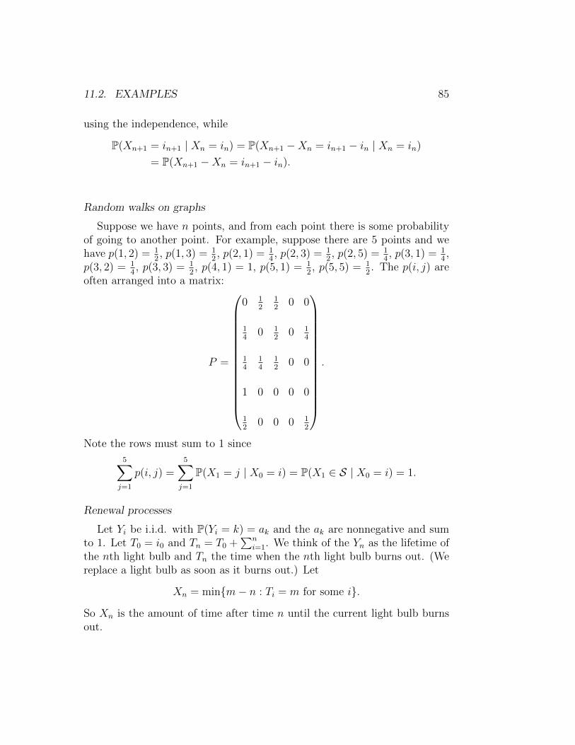
11.2. EXAMPLES 85

using the independence, while

P(Xn+1 = in+1 | Xn = in) = P(Xn+1 −Xn = in+1 − in | Xn = in)

= P(Xn+1 −Xn = in+1 − in).

Random walks on graphs

Suppose we have n points, and from each point there is some probabilityof going to another point. For example, suppose there are 5 points and wehave p(1, 2) = 1

2, p(1, 3) = 1

2, p(2, 1) = 1

4, p(2, 3) = 1

2, p(2, 5) = 1

4, p(3, 1) = 1

4,

p(3, 2) = 14, p(3, 3) = 1

2, p(4, 1) = 1, p(5, 1) = 1

2, p(5, 5) = 1

2. The p(i, j) are

often arranged into a matrix:

P =

0 12

12

0 0

14

0 12

0 14

14

14

12

0 0

1 0 0 0 0

12

0 0 0 12

.

Note the rows must sum to 1 since

5∑j=1

p(i, j) =5∑j=1

P(X1 = j | X0 = i) = P(X1 ∈ S | X0 = i) = 1.

Renewal processes

Let Yi be i.i.d. with P(Yi = k) = ak and the ak are nonnegative and sumto 1. Let T0 = i0 and Tn = T0 +

∑ni=1. We think of the Yn as the lifetime of

the nth light bulb and Tn the time when the nth light bulb burns out. (Wereplace a light bulb as soon as it burns out.) Let

Xn = minm− n : Ti = m for some i.

So Xn is the amount of time after time n until the current light bulb burnsout.


If Xn = j and j > 0, then Ti = n + j for some i but Ti does not equaln, n+ 1, . . . , n+ j − 1 for any i. So Ti = (n+ 1) + (j − 1) for some i and Tidoes not equal (n+ 1), (n+ 1) + 1, . . . , (n+ 1) + (j − 2) for any i. ThereforeXn+1 = j − 1. So p(i, i− 1) = 1 if i ≥ 1.

If Xn = 0, then a light bulb burned out at time n and Xn+1 is 0 if the nextlight bulb burned out immediately and j − 1 if the light bulb has lifetime j.The probability of this is aj. So p(0, j) = aj+1. All the other p(i, j)’s are 0.

Branching processes

Consider k particles. At the next time interval, some of them die, and someof them split into several particles. The probability that a given particle willsplit into j particles is given by aj, j = 0, 1, . . ., where the aj are nonnegativeand sum to 1. The behavior of each particle is independent of the behaviorof all the other particles. If Xn is the number of particles at time n, then Xn

is a Markov chain. Let Yi be i.i.d. random variables with P(Yi = j) = aj.The p(i, j) for Xn are somewhat complicated, and can be defined by p(i, j) =P(∑i

m=1 Ym = j).

Queues

We will discuss briefly the M/G/1 queue. The M refers to the fact thatthe customers arrive according to a Poisson process. So the probability thatthe number of customers arriving in a time interval of length t is k is given bye−λt(λt)k/k! The G refers to the fact that the length of time it takes to servea customer is given by a distribution that is not necessarily exponential. The1 refers to the fact that there is 1 server.

Suppose the length of time to serve one customer has distribution functionF with density f . The probability that k customers arrive during the timeit takes to serve one customer is

ak =

∫ ∞0

e−λt(λt)k

k!f(t) dt.

Let the Yi be i.i.d. with P(Yi = k−1) = ak. So Yi is the number of customersarriving during the time it takes to serve one customer. Let Xn+1 = (Xn +Yn+1)

+ be the number of customers waiting. Then Xn is a Markov chainwith p(0, 0) = a0 + a1 and p(i, i− 1 + k) = ak if i ≥ 1, k > 1.

Ehrenfest urns

11.3. MARKOV PROPERTIES 87

Suppose we have two urns with a total of r balls, k in one and r − k inthe other. Pick one of the r balls at random and move it to the other urn.Let Xn be the number of balls in the first urn. Xn is a Markov chain withp(k, k + 1) = (r − k)/r, p(k, k − 1) = k/r, and p(i, j) = 0 otherwise.

One model for this is to consider two containers of air with a thin tubeconnecting them. Suppose a few molecules of a foreign substance are in-troduced. Then the number of molecules in the first container is like anEhrenfest urn. We shall see that all states in this model are recurrent, soinfinitely often all the molecules of the foreign substance will be in the firsturn. Yet there is a tendency towards equilibrium, so on average there will beabout the same number of molecules in each container for all large times.

Birth and death processes

Suppose there are i particles, and the probability of a birth is ai, theprobability of a death is bi, where ai, bi ≥ 0, ai + bi ≤ 1. Setting Xn equalto the number of particles, then Xn is a Markov chain with p(i, i + 1) = ai,p(i, i− 1) = bi, and p(i, i) = 1− ai − bi.

11.3 Markov properties

Proposition 11.3 Px(Xn+1 = z | X1, . . . , Xn) = PXn(X1 = z), Px-a.s.

Proof. The right hand side is measurable with respect to the σ-field gener-ated by Xn. We therefore need to show that if A is in σ(Xn), then

Px(Xn+1 = z, A) = E x[PXn(X1 = z);A].

A is of the form (Xn ∈ B) for some B ⊂ S, so it suffices to show

Px(Xn+1 = z,Xn = y) = E x[PXn(X1 = z);Xn = y] (11.6)

and sum over y ∈ B.

Note the right hand side of (11.6) is equal to

E x[Py(X1 = z);Xn = y],


while

Py(X1 = z) =∑i

Py(X0 = i,X1 = z) =∑i

1y(i)p(i, z) = p(y, z).

Therefore the right hand side of (11.6) is

p(y, z)Px(Xn = y).

On the other hand, the left hand side of (11.6) equals

Px(Xn+1 = z | Xn = y)Px(Xn = y) = p(y, z)Px(Xn = y).

Theorem 11.4

Px(Xn+1 = i1, . . . , Xn+m = im | X1, . . . , Xn) = PXn(X1 = i1, . . . , Xm = im).

Proof. Note this is equivalent to

E x[f1(Xn+1) · · · fm(Xn+m) | X1, . . . , Xn] = EXn [f1(X1) · · · fm(Xm)].

To go one way, we let fk = 1ik, to go the other, we multiply the conditionalprobability result by f1(i1) · · · fm(im) and sum over all possible values ofi1, . . . , im.

We’ll use induction. The case m = 1 is the previous proposition. Let ussuppose the result holds for m and prove that it holds for m+ 1. Let

C = (Xn+1 = i1, . . . , Xn+m−1 = im−1)

andD = (X1 = i1, . . . , Xm−1 = im−1).

Setϕ(z) = Pz(X1 = im+1).

Let Fn = σ(X1, . . . , Xn). We then have

Px(Xn+1 = i1, . . . , Xn+m = im, Xn+m+1 = im+1 | Fn)

= E x[Px(C,Xn+m = im, Xn+m+1 = im+1 | Fn+m) | Fn]

= E x[1C1im(Xn+m)Px(Xn+m+1 = im+1 | Fn+m) | Fn]

= E x[1C(ϕ1im)(Xn+m) | Fn].

11.3. MARKOV PROPERTIES 89

By the induction hypothesis, this is equal to

EXn [1D(ϕ1im)(Xm)].

For any y,

E y[1D(ϕ1im)(Xm)]

= E y[1D1im(Xm)PXm(X1 = im+1)]

= E y[1D1im(Xm)Py(Xm+1 = im+1 | Fm)]

= E y[1D1im(Xm)1im+1(Xm+1)].

The strong Markov property is the same as the Markov property, butwhere the fixed time n is replaced by a stopping time N .

Theorem 11.5 If N is a finite stopping time, then

Px(XN+1 = i1 | FN) = PXN (X1 = i1),

and

Px(XN+1 = i1, . . . , XN+m = im | FN) = PXN (X1 = i1, . . . , Xm = im),

both Px-a.s.

Proof. We will show

Px(XN+1 = j | FN) = PXN (X1 = j).

Once we have this, we can proceed as in the proof of the previous theoremto obtain the second result. To show the above equality, we need to showthat if B ∈ FN , then

Px(XN+1 = j, B) = E x[PXN (X1 = j);B]. (11.7)

Recall that since B ∈ FN , then B ∩ (N = k) ∈ Fk. We have

Px(XN+1 = j, B,N = k) = Px(Xk+1 = j, B,N = k)

= E x[Px(Xk+1 = j | Fk);B,N = k]

= E x[PXk(X1 = j);B,N = k]

= E x[PXN (X1 = j);B,N = k].


Now sum over k; since N is finite, we obtain our desired result.

We will need the following corollary. We use the notation Ty = minn >0 : Xn = y, the first time the Markov chain hits the state y.

Corollary 11.6 Let U be a finite stopping time. Let V = minn > U :Xn = y, the first time after U that the chain hits y. Then

Px(V <∞ | FU) = PXU (Ty <∞).

Proof. We can write

(V <∞) = ∪∞n=1(V = U + n)

= ∪∞n=1(XU+1 6= y, . . . , XU+n−1 6= y,XU+n = y).

By the theorem

Px(XU+1 6= y, . . . ,XU+n−1 6= y,XU+n = y)

= PXU (X1 6= y, . . . , Xn−1 6= y,Xn = y)

= PXU (Ty = n).

Now sum over n.

Another way of expressing the Markov property is through the Chapman-Kolmogorov equations. Let pn(i, j) = P(Xn = j | X0 = i).

Proposition 11.7 For all i, j,m, n we have

pn+m(i, j) =∑k∈S

pn(i, k)pm(k, j).

Proof. We write

P(Xn+m = j,X0 = i) =∑k

P(Xn+m = j,Xn = k,X0 = i)

=∑k

P(Xn+m = j | Xn = k,X0 = i)P(Xn = k | X0 = i)P(X0 = i)

=∑k

P(Xn+m = j | Xn = k)pn(i, k)P(X0 = i)

=∑k

pm(k, j)pn(i, k)P(X0 = i).

11.4. RECURRENCE AND TRANSIENCE 91

If we divide both sides by P(X0 = i), we have our result.

Note the resemblance to matrix multiplication. It is clear if P is thematrix made up of the p(i, j), then P n will be the matrix whose (i, j) entryis pn(i, j).

11.4 Recurrence and transience

LetTy = mini > 0 : Xi = y.

This is the first time that Xi hits the point y. Even if X0 = y we would haveTy > 0. We let T ky be the k-th time that the Markov chain hits y and we set

r(x, y) = Px(Ty <∞),

the probability starting at x that the Markov chain ever hits y.

Proposition 11.8 Px(T ky <∞) = r(x, y)r(y, y)k−1.

Proof. The case k = 1 is just the definition, so suppose k > 1. Let U = T k−1y

and let V be the first time the chain hits y after U . Using the corollary tothe strong Markov property,

Px(T ky <∞) = Px(V <∞, T k−1y <∞)

= E x[Px(V <∞ | FTk−1y

);T k−1y <∞]

= E x[PX(Tk−1y )(Ty <∞);T k−1y <∞]

= E x[Py(Ty <∞);T k−1y <∞]

= r(y, y)Px(T k−1y <∞).

We used here the fact that at time T k−1y the Markov chain must be at thepoint y. Repeating this argument k − 2 times yields the result.

We say that y is recurrent if r(y, y) = 1; otherwise we say y is transient.Let

N(y) =∞∑n=1

1(Xn=y).


Proposition 11.9 y is recurrent if and only if E yN(y) =∞.

Proof. Note

E yN(y) =∞∑k=1

Py(N(y) ≥ k) =∞∑k=1

Py(T ky <∞)

=∞∑k=1

r(y, y)k.

We used the fact that N(y) is the number of visits to y and the number ofvisits being larger than k is the same as the time of the k-th visit being finite.Since r(y, y) ≤ 1, the left hand side will be finite if and only if r(y, y) < 1.

Observe that

E yN(y) =∑n

Py(Xn = y) =∑n

pn(y, y).

If we consider simple symmetric random walk on the integers, then pn(0, 0)

is 0 if n is odd and equal to

(nn/2

)2−n if n is even. This is because in order

to be at 0 after n steps, the walk must have had n/2 positive steps and n/2negative steps; the probability of this is given by the binomial distribution.Using Stirling’s approximation, we see that pn(0, 0) ∼ c/

√n for n even, which

diverges, and so simple random walk in one dimension is recurrent.

Similar arguments show that simple symmetric random walk is also recur-rent in 2 dimensions but transient in 3 or more dimensions.

Proposition 11.10 If x is recurrent and r(x, y) > 0, then y is recurrentand r(y, x) = 1.

Proof. First we show r(y, x) = 1. Suppose not. Since r(x, y) > 0, thereis a smallest n and y1, . . . , yn−1 such that p(x, y1)p(y1, y2) · · · p(yn−1, y) > 0.Since this is the smallest n, none of the yi can equal x. Then

Px(Tx =∞) ≥ p(x, y1) · · · p(yn−1, y)(1− r(y, x)) > 0,

11.4. RECURRENCE AND TRANSIENCE 93

a contradiction to x being recurrent.

Next we show that y is recurrent. Since r(y, x) > 0, there exists L suchthat pL(y, x) > 0. Then

pL+n+K(y, y) ≥ pL(y, x)pn(x, x)pK(x, y).

Summing over n,∑n

pL+n+K(y, y) ≥ pL(y, x)pK(x, y)∑n

pn(x, x) =∞.

We say a subset C of S is closed if x ∈ C and r(x, y) > 0 implies y ∈ C.A subset D is irreducible if x, y ∈ D implies r(x, y) > 0.

Proposition 11.11 Let C be finite and closed. Then C contains a recurrentstate.

From the preceding proposition, if C is irreducible, then all states will berecurrent.

Proof. If not, for all y we have r(y, y) < 1 and

E xN(y) =∞∑k=1

Px(N(y) ≥ k) =∞∑k=1

Px(T ky <∞)

=∞∑k=1

r(x, y)r(y, y)k−1 =r(x, y)

1− r(y, y)<∞.

Since C is finite, then∑

y ExN(y) <∞. But that is a contradiction since∑

y

E xN(y) =∑y

∑n

pn(x, y) =∑n

∑y

pn(x, y)

=∑n

Px(Xn ∈ C) =∑n

1 =∞.


Theorem 11.12 Let R = x : r(x, x) = 1, the set of recurrent states.Then R = ∪∞i=1Ri, where each Ri is closed and irreducible.

Proof. Say x ∼ y if r(x, y) > 0. Since every state is recurrent, x ∼ x and ifx ∼ y, then y ∼ x. If x ∼ y and y ∼ z, then pn(x, y) > 0 and pm(y, z) > 0for some n and m. Then pn+m(x, z) > 0 or x ∼ z. Therefore we have anequivalence relation and we let the Ri be the equivalence classes.

Looking at our examples, it is easy to see that in the Ehrenfest urn modelall states are recurrent. For the branching process model, suppose p(x, 0) > 0for all x. Then 0 is recurrent and all the other states are transient. In therenewal chain, there are two cases. If k : ak > 0 is unbounded, all statesare recurrent. If K = maxk : ak > 0, then 0, 1, . . . , K − 1 are recurrentstates and the rest are transient.

For the queueing model, let µ =∑kak, the expected number of people

arriving during one customer’s service time. We may view this as a branchingprocess by letting all the customers arriving during one person’s service timebe considered the progeny of that customer. It turns out that if µ ≤ 1, 0 isrecurrent and all other states are also. If µ > 1 all states are transient.

11.5 Stationary measures

A probability µ is a stationary distribution if∑x

µ(x)p(x, y) = µ(y). (11.8)

In matrix notation this is µP = µ, or µ is the left eigenvector corresponding tothe eigenvalue 1. In the case of a stationary distribution, Pµ(X1 = y) = µ(y),which implies that X1, X2, . . . all have the same distribution. We can use(11.8) when µ is a measure rather than a probability, in which case it iscalled a stationary measure. Note

µP n = (µP )P n−1 = µP n−1 = · · · = µ.

If we have a random walk on the integers, µ(x) = 1 for all x serves as astationary measure. In the case of an asymmetric random walk: p(i, i+ 1) =

11.5. STATIONARY MEASURES 95

p, p(i, i − 1) = q = 1 − p and p 6= q, setting µ(x) = (p/q)x also works. Tocheck this, note

µP (x) =∑

µ(i)p(i, x) = µ(x− 1)p(x− 1, x) + µ(x+ 1)p(x+ 1, x)

=(pq

)x−1p+

(pq

)x+1

q

=px

qx· q +

px

qx· q =

px

qx.

In the Ehrenfest urn model, µ(x) = 2−r(rx

)works. One way to see this

is that µ is the distribution one gets if one flips r coins and puts a coin inthe first urn when the coin is heads. A transition corresponds to picking acoin at random and turning it over.

Proposition 11.13 Let a be recurrent and let T = Ta. Set

µ(y) = E aT−1∑n=0

1(Xn=y).

Then µ is a stationary measure.

The idea of the proof is that µ(y) is the expected number of visits to yby the sequence X0, . . . , XT−1 while µP is the expected number of visits toy by X1, . . . , XT . These should be the same because XT = X0 = a.

Proof. Let pn(a, y) = Pa(Xn = y, T > n). So

µ(y) =∞∑n=0

Pa(Xn = y, T > n) =∞∑n=0

pn(a, y)

and ∑y

µ(y)p(y, z) =∑y

∞∑n=0

pn(a, y)p(y, z).


First we consider the case z 6= a. Then∑y

pn(a, y)p(y, z)

=∑y

Pa(hit y in n steps without first hitting a

and then go to z in one step)

= pn+1(a, z).

So ∑y

µ(y)p(y, z) =∑n

∑y

pn(a, y)p(y, z)

=∞∑n=0

pn+1(a, z) =∞∑n=0

pn(a, z)

= µ(z)

since p0(a, z) = 0.

Second we consider the case a = z. Then∑y

pn(a, y)p(y, z)

=∑y

Pa(hit y in n steps without first hitting a

and then go to z in one step)

= Pa(T = n+ 1).

Recall Pa(T = 0) = 0, and since a is recurrent, T <∞. So∑y

µ(y)p(y, z) =∑n

∑y

pn(a, y)p(y, z)

=∞∑n=0

Pa(T = n+ 1) =∞∑n=0

Pa(T = n) = 1.

On the other hand,T−1∑n=0

1(Xn=a) = 1(X0=a) = 1,


hence µ(a) = 1. Therefore, whether z 6= a or z = a, we have µP (z) = µ(z).

Finally, we show µ(y) < ∞. If r(a, y) = 0, then µ(y) = 0. If r(a, y) > 0,choose n so that pn(a, y) > 0, and then

1 = µ(a) =∑y

µ(y)pn(a, y),

which implies µ(y) <∞.

We next turn to uniqueness of the stationary distribution. We give thestationary measure constructed in Proposition 11.13 the name µa. We showedµa(a) = 1.

Proposition 11.14 If the Markov chain is irreducible and all states are re-current, then the stationary measure is unique up to a constant multiple.

Proof. Fix a ∈ S. Let µa be the stationary measure constructed above andlet ν be any other stationary measure.

Since ν = νP , then

ν(z) = ν(a)p(a, z) +∑y 6=a

ν(y)p(y, z)

= ν(a)p(a, z) +∑y 6=a

ν(a)p(a, y)p(y, z) +∑x 6=a

∑y 6=a

ν(x)p(x, y)p(y, z)

= ν(a)Pa(X1 = z) + ν(a)Pa(X1 6= a,X2 = z)

+ Pν(X0 6= a,X1 6= a,X2 = z).

Continuing,

ν(z) = ν(a)n∑

m=1

Pa(X1 6= a,X2 6= a, . . . , Xm−1 6= a,Xm = z)

+ Pν(X0 6= a,X1 6= a, . . . , Xn−1 6= a,Xn = z)

≥ ν(a)n∑

m=1

Pa(X1 6= a,X2 6= a, . . . , Xm−1 6= a,Xm = z).


Letting n→∞, we obtain

ν(z) ≥ ν(a)µa(z).

We have

ν(a) =∑x

ν(x)pn(x, a) ≥ ν(a)∑x

µa(x)pn(x, a)

= ν(a)µa(a) = ν(a),

since µa(a) = 1 (see proof of Proposition 11.13). This means that we haveequality and so for each n and x either pn(x, a) = 0 or

ν(x) = ν(a)µa(x).

Since r(x, a) > 0, thhen pn(x, a) > 0 for some n. Consequently

ν(x)

ν(a)= µa(x).

Proposition 11.15 If a stationary distribution exists, then µ(y) > 0 impliesy is recurrent.

Proof. If µ(y) > 0, then

∞ =∞∑n=1

µ(y) =∞∑n=1

∑x

µ(x)pn(x, y) =∑x

µ(x)∞∑n=1

pn(x, y)

=∑x

µ(x)∞∑n=1

Px(Xn = y) =∑x

µ(x)E xN(y)

=∑x

µ(x)r(x, y)[1 + r(y, y) + r(y, y)2 + · · · ].

Since r(x, y) ≤ 1 and µ is a probability measure, this is less than∑x

µ(x)(1 + r(y, y) + · · · ) ≤ 1 + r(y, y) + · · · .

Hence r(y, y) must equal 1.

Recall that Tx is the first time to hit x.


Proposition 11.16 If the Markov chain is irreducible and has stationarydistribution µ, then

µ(x) =1

E xTx.

Proof. µ(x) > 0 for some x. If y ∈ S, then r(x, y) > 0 and so pn(x, y) > 0for some n. Hence

µ(y) =∑x

µ(x)pn(x, y) > 0.

Hence by Proposition 11.15, all states are recurrent. By the uniqueness of thestationary distribution, µx is a constant multiple of µ, i.e., µx = cµ. Recall

µx(y) =∞∑n=0

Px(Xn = y, Tx > n),

and so∑y

µx(y) =∑y

∞∑n=0

Px(Xn = y, Tx > n) =∑n

∑y

Px(Xn = y, Tx > n)

=∑n

Px(Tx > n) = E xTx.

Thus c = E xTx. Recalling that µx(x) = 1,

µ(x) =µx(x)

c=

1

E xTx.

We make the following distinction for recurrent states. If E xTx <∞, thenx is said to be positive recurrent. If x is recurrent but E xTx = ∞, x is nullrecurrent.

An example of null recurrent states is the simple random walk on theintegers. If we let g(y) = E yTx, the Markov property tells us that

g(y) = 1 + 12g(y − 1) + 1

2g(y + 1).

Some algebra translates this to

g(y)− g(y − 1) = 2 + g(y + 1)− g(y).


If d(y) = g(y) − g(y − 1), we have d(y + 1) = d(y) − 2. If d(y0) is finite forany y0, then g(y) will be less than −1 for all y larger than some y1, whichimplies that g(y) will be negative for sufficiently large y, a contradiction. Weconclude g is identically infinite.

Proposition 11.17 Suppose a chain is irreducible.(a) If there exists a positive recurrent state, then there is a stationary distri-bution.(b) If there is a stationary distribution, all states are positive recurrent.(c) If there exists a transient state, all states are transient.(d) If there exists a null recurrent state, all states are null recurrent.

Proof. To show (a), suppose x is positive recurrent. We have seen that

µx(y) = E xTx−1∑n=0

1(Xn=y)

is a stationary measure. Then

µx(S) =∑y

µx(y) = E xTx−1∑n=0

1 = E xTx <∞.

Therefore µ(y) = µ(y)/E xTx will be a stationary distribution. From thedefinition of µx we have µx(x) = 1, hence µ(x) > 0.

For (b), suppose µ(x) > 0 for some x. If y is another state, choose n sothat pn(x, y) > 0, and then from

µ(y) =∑x

µ(x)pn(x, y)

we conclude that µ(y) > 0. Then 0 < µ(y) = 1/E yTy, which implies E yTy <∞.

We showed that if x is recurrent and r(x, y) > 0, then y is recurrent. So(c) follows.

Suppose there exists a null recurrent state. If there exists a positive re-current or transient state as well, then by (a) and (b) or by (c) all states arepositive recurrent or transient, a contradiction, and (d) follows.

11.6. CONVERGENCE 101

11.6 Convergence

Our goal is to show that under certain conditions pn(x, y) → π(y), where πis the stationary distribution. (In the null recurrent case pn(x, y)→ 0.)

Consider a random walk on the set 0, 1, where with probability one oneach step the chain moves to the other state. Then pn(x, y) = 0 if x 6= y andn is even. A less trivial case is the simple random walk on the integers. Weneed to eliminate this periodicity.

Suppose x is recurrent, let Ix = n ≥ 1 : pn(x, x) > 0, and let dx be theg.c.d. (greatest common divisor) of Ix. dx is called the period of x.

Proposition 11.18 If r(x, y) > 0, then dy = dx.

Proof. Since x is recurrent, r(y, x) > 0. Choose K and L such thatpK(x, y), pL(y, x) > 0.

pK+L+n(y, y) ≥ pL(y, x)pn(x, x)pK(x, y),

so taking n = 0, we have pK+L(y, y) > 0, or dy divides K + L. So dy dividesn if pn(x, x) > 0, or dy is a divisor of Ix. Hence dy divides dx. By symmetrydx divides dy.

Proposition 11.19 If dx = 1, there exists m0 such that pm(x, x) > 0 when-ever m ≥ m0.

Proof. First of all, Ix is closed under addition: if m,n ∈ Ix,

pm+n(x, x) ≥ pm(x, x)pn(x, x) > 0.

Secondly, if there exists N such that N,N + 1 ∈ Ix, let m0 = N2. Ifm ≥ m0, then m−N2 = kN + r for some r < N and

m = r +N2 + kN = r(N + 1) + (N − r + k)N ∈ Ix.

Third, pick n0 ∈ Ix and k > 0 such that n0 + k ∈ Ix. If k = 1, we aredone. Since dx = 1, there exists n1 ∈ Ix such that k does not divide n1.


We have n1 = mk + r for some 0 < r < k. Note (m + 1)(n0 + k) ∈ Ixand (m + 1)n0 + n1 ∈ Ix. The difference between these two numbers is(m + 1)k − n1 = k − r < k. So now we have two numbers in Ik differing byless than or equal to k − 1. Repeating at most k times, we get two numbersin Ix differing by at most 1, and we are done.

We write d for dx. A chain is aperiodic if d = 1.

If d > 1, we say x ∼ y if pkd(x, y) > 0 for some k > 0 We divide S intoequivalence classes S1, . . .Sd. Every d steps the chain started in Si is back inSi. So we look at p′ = pd on Si.

Theorem 11.20 Suppose the chain is irreducible, aperiodic, and has a sta-tionary distribution π. Then pn(x, y)→ π(y) as n→∞.

Proof. The idea is to take two copies of the chain with different startingdistributions, let them run independently until they couple, i.e., hit eachother, and then have them move together. So define

q((x1, y1), (x2, y2)) =

p(x1, x2)p(y1, y2) if x1 6= y1,

p(x1, x2) if x1 = y1, x2 = y2,

0 otherwise.

Let Zn = (Xn, Yn) and T = mini : Xi = Yi. We have

P(Xn = y) = P(Xn = y, T ≤ n) + P(Xn = y, T > n)

= P(Yn = y, T ≤ n) + P(Xn = y, T > n),

whileP(Yn = y) = P(Yn = y, T ≤ n) + P(Yn = y, T > n).

Subtracting,

P(Xn = y)− P(Yn = y) ≤ P(Xn = y, T > n)− P(Yn = y, T > n)

≤ P(Xn = y, T > n) ≤ P(T > n).

Using symmetry,

|P(Xn = y)− P(Yn = y)| ≤ P(T > n).

11.6. CONVERGENCE 103

Suppose we let Y0 have distribution π and X0 = x. Then

|pn(x, y)− π(y)| ≤ P(T > n).

It remains to show P(T > n) → 0. To do this, consider another chainWn = (Xn, Yn), where now we take Xn, Yn independent. Define

r((x1, y1), (x2, y2)) = p(x1, x2)p(y1, y2).

The chain under the transition probabilities r is irreducible. To see this,there exist K and L such that pK(x1, x2) > 0 and pL(y1, y2) > 0. If M islarge, pL+M(x2, x2) > 0 and pK+M(y2, y2) > 0. So pK+L+M(x1, x2) > 0 andpK+L+M(y1, y2) > 0, and hence we have rK+L+M((x1, x2), (y1, y2)) > 0.

It is easy to check that π′(a, b) = π(a)π(b) is a stationary distribution forW . Hence Wn is recurrent, and hence it will hit (x, x), hence the time to hitthe diagonal (y, y) : y ∈ S is finite. However the distribution of the timeto hit the diagonal is the same as T .


Documents

Probability Theory - Rich Bass home pagebass.math.uconn.edu/gradprob.pdf · Chapter 1 Basic notions 1.1 A few de nitions from measure theory Given a set X, a ˙-algebra on Xis a collection