Probability Theory Review

Belief representation: how do we represent our belief (hypothesis) of where the robot is located?Continuous map with single hypothesis probability distribution

Continuous map with multiple hypotheses probability distribution

Discretized map with multiple hypotheses probability distribution

Discretized topological map with with multiple hypotheses probability distribution

Belief representation

• Single-hypothesis belief: The robot’s belief about its position is expressed as a single point on a map• Advantage: no ambiguity, simplifies planning and decision making• Disadvantage: does not represent ambiguity/uncertainty

• Multi-hypothesis belief: allows the robot to track (possibly infinitely) many possible positions.

In both of the above, the beliefs are represented as probabilities

Discrete Random Variables

• X denotes a random variable.

• X can take on a finite number of values in {x1, x2, …, xn}.

• P(X=xi), or P(xi), is the probability that the random variable Xtakes on value xi.

• P(xi) is called probability mass function.

• E.g.2.0)( =RainingP

Continuous Random Variables

• 𝑋 takes on values in the continuum.

• 𝑝(𝑋 = 𝑥), or 𝑝(𝑥), is a probability density function.

• E.g.

ò=Îb

a

dxxpbaxP )()),((

x

p(x)

Probability Density Function

Since continuous probability functions are defined for an infinite number of points over a continuous interval, the probability at a single point is always 0.

x

p(x)Magnitude of curve could be greater than 1 in some areas. The total area under the curve must add up to 1.

Joint Probability

• Notation• 𝑃(𝑋 = 𝑥 𝑎𝑛𝑑 𝑌 = 𝑦) = 𝑃(𝑥, 𝑦)

• If X and Y are independent then 𝑃(𝑥, 𝑦) = 𝑃(𝑥) 𝑃(𝑦)

Conditional Probability

• 𝑃(𝑥 | 𝑦) is the probability of x given y

𝑃(𝑥 | 𝑦) = / 0,1/ 1

𝑃(𝑥, 𝑦) = 𝑃(𝑥 | 𝑦) 𝑃(𝑦)= 𝑃(𝑦 | 𝑥) 𝑃(𝑥)

• If X and Y are independent then𝑃(𝑥 | 𝑦) = 𝑃(𝑥)

An ExampleRoll two dice, observe 𝑥2and 𝑥3.We know that there are 36 possible outcomes, all of which are equally likely (assuming the dice are fair).It’s easy to compute probabilities by simply counting outcomes:• Probability 𝑥2 = 6:

6,1 , 6,2 , 6,3 , 6,4 , 6,5 , (6,6) → 𝑃 =636

=16

• Probability 𝑥2 = 6 and 𝑥3 is even:6,2 , 6,4 , (6,6) → 𝑃 =

336 =

112

• Probability 𝑥2is even:

(2,1), (2,2), (2,3), (2,4), (2,5), (2,6)(4,1), (4,2), (4,3), (4,4), (4,5), (4,6)(6,1), (6,2), (6,3), (6,4), (6,5), (6,6)

→ 𝑃 =1836

=12

Let’s apply rules of conditional and joint probabilities:Define events: 𝐴: x2 is even; 𝐵: x2 = 6; 𝐶: x3is even; 𝐷: x3 = 5From the previous page, we easily compute the following:

𝑃 𝐴 =12 , 𝑃 𝐵 =

16 , 𝑃 𝐶 =

12 , 𝑃 𝐷 =

16 .

Let’s look at some combinations of events:

• 𝑃 𝐴, 𝐵 = 2C ≠ 𝑃 𝐴 𝑃 𝐵 = 2

C×23 =

223 → NOT independent

• 𝑃 𝐴, 𝐶 = FGC = 𝑃 𝐴 𝑃 𝐶 = 2

3×23 → independent

• 𝑃 𝐵|𝐴 = /(H,I)/(H) =

JKJL= 2

G

This agrees with our intuition, since x2 = 6 in one third of the cases of x2being even:(2,1), (2,2), (2,3), (2,4), (2,5), (2,6)(4,1), (4,2), (4,3), (4,4), (4,5), (4,6)(6,1), (6,2), (6,3), (6,4), (6,5), (6,6)

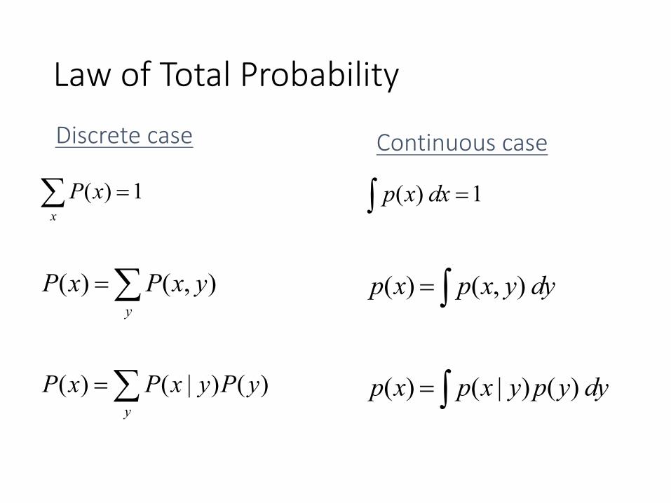
Law of Total Probability

å=y

yxPxP ),()(

å=y

yPyxPxP )()|()(

å =x

xP 1)(

Discrete case

ò =1)( dxxp

Continuous case

ò= dyypyxpxp )()|()(

ò= dyyxpxp ),()(

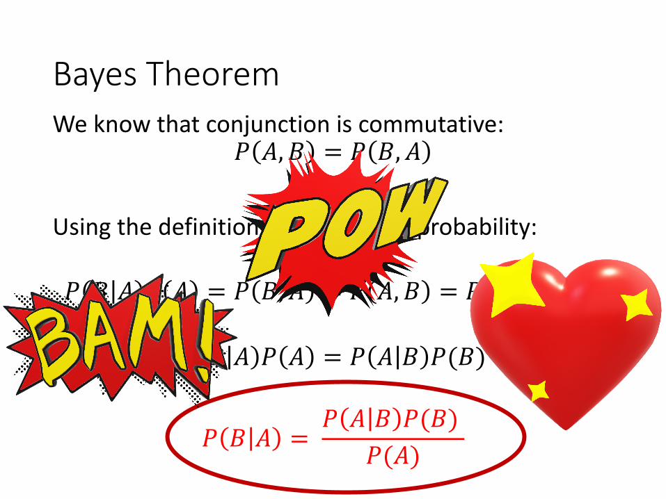
Bayes TheoremWe know that conjunction is commutative:

𝑃 𝐴, 𝐵 = 𝑃 𝐵, 𝐴

Using the definition of conditional probability:

𝑃 𝐵 𝐴 𝑃 𝐴 = 𝑃 𝐵, 𝐴 = 𝑃 𝐴, 𝐵 = 𝑃 𝐴 𝐵 𝑃 𝐵

𝑃 𝐵 𝐴 𝑃 𝐴 = 𝑃 𝐴 𝐵 𝑃(𝐵)

𝑃 𝐵 𝐴 =𝑃 𝐴 𝐵 𝑃(𝐵)

𝑃(𝐴)

Bayes TheoremWe know that conjunction is commutative:

𝑃 𝐴, 𝐵 = 𝑃 𝐵, 𝐴

Using the definition of conditional probability:

𝑃 𝐵 𝐴 𝑃 𝐴 = 𝑃 𝐵, 𝐴 = 𝑃 𝐴, 𝐵 = 𝑃 𝐴 𝐵 𝑃 𝐵

𝑃 𝐵 𝐴 𝑃 𝐴 = 𝑃 𝐴 𝐵 𝑃(𝐵)

𝑃 𝐵 𝐴 =𝑃 𝐴 𝐵 𝑃(𝐵)

𝑃(𝐴)

Example

We roll one die, and an observer tells us things about the outcome. We want to know if 𝑋 = 4.

• Before we know anything, we believe 𝑃 𝑋 = 4 = 2C. PRIOR

• Now, suppose the observer tells us that 𝑋is even. EVIDENCE

𝑃 𝑋 = 4 𝑋 even) = /(PQR,P STSU)/(P STSU)

=JKJL= 2

GBAYES

• We could also use Bayes to infer 𝑃 𝑋 = even 𝑋 = 4):

𝑃 𝑋 even 𝑋 = 4) =𝑃(𝑋 = 4, 𝑋 even)

𝑃(𝑋 = 4)=1616= 1

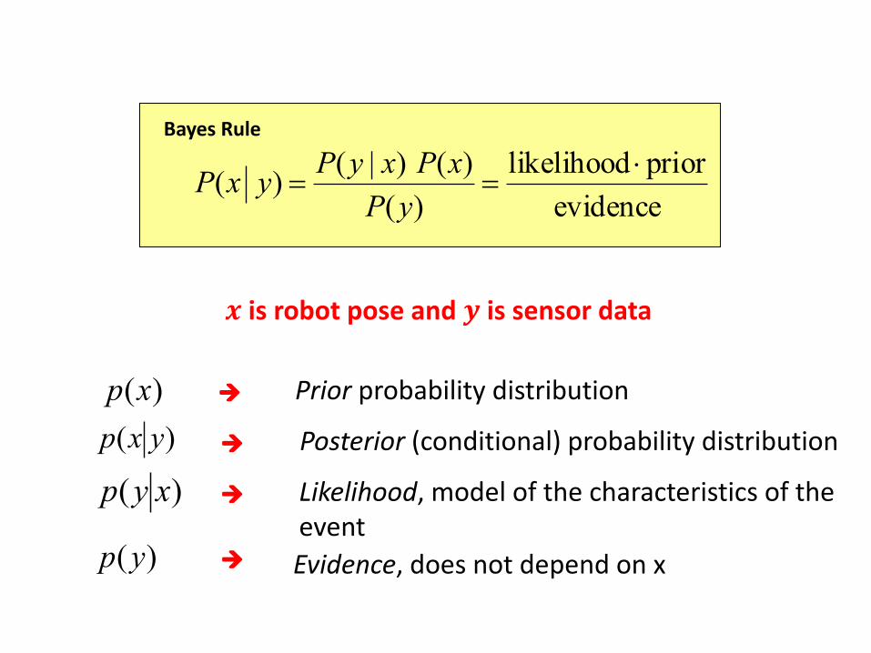
)( yxp

evidenceprior likelihood

)()()|()( ×==

yPxPxyPyxP

Posterior (conditional) probability distribution

)( xyp

)(xp Prior probability distribution

Likelihood, model of the characteristics of the event

)(yp

à

à

à

à

Evidence, does not depend on x

Bayes Rule

𝒙 is robot pose and 𝒚 is sensor data

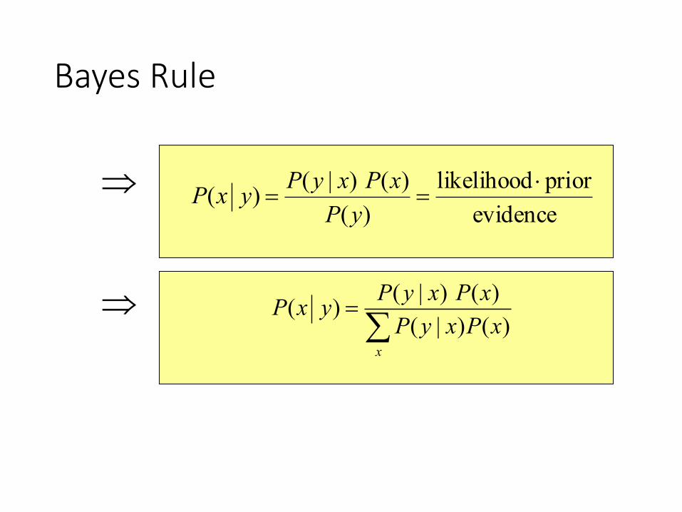
Bayes Rule

evidenceprior likelihood

)()()|()( ×==

yPxPxyPyxPÞ

å=

xxPxyPxPxyPyxP)()|()()|()(Þ

About likelihoods…

Why do we call the conditional probability 𝑝(𝑦|𝑥) a likelihood, but we call 𝑝(𝑥|𝑦) the posterior??

We define the likelihood ℒ(𝑥) to be a function of 𝑥, not a function of 𝑦 :

ℒ 𝑥 = 𝑝 𝑦 𝑥

Note: ℒ 𝑥 is not a probability. In particular,

Y0

ℒ 𝑥 ≠ 1

Normalization Coefficient

𝑃 𝑥 𝑧 =𝑃 𝑧 𝑥 𝑃(𝑥)

𝑃(𝑧)

Note that the denominator is independent of 𝑥, and as a result will typically be the same for any value of 𝑥in the posterior 𝑃 𝑥 𝑧 .

Therefore, we typically represent the normalization term by the coefficient 𝜂 = [𝑃 𝑧 ]^2 and Bayes equation is written as

𝑃 𝑥 𝑧 = 𝜂𝑃 𝑧 𝑥 𝑃(𝑥)

Simple Example of State Estimation

• Suppose a robot obtains measurement 𝑧 (e.g., distance sensor reports an obstacle 40cm in front of the robot)• What is 𝑃(𝑜𝑝𝑒𝑛|𝑧)?

Causal vs. Diagnostic Reasoning

• 𝑃(𝑜𝑝𝑒𝑛|𝑧) is diagnostic.• 𝑃(𝑧|𝑜𝑝𝑒𝑛) is causal.• Often causal knowledge is easier to obtain.• Bayes rule allows us to use causal knowledge:

)()()|()|( zP

openPopenzPzopenP =

Comes from sensor model.

Use law of total probability: 𝑃 𝑧 = ∑1𝑃 𝑧 𝑦 𝑃(𝑦)

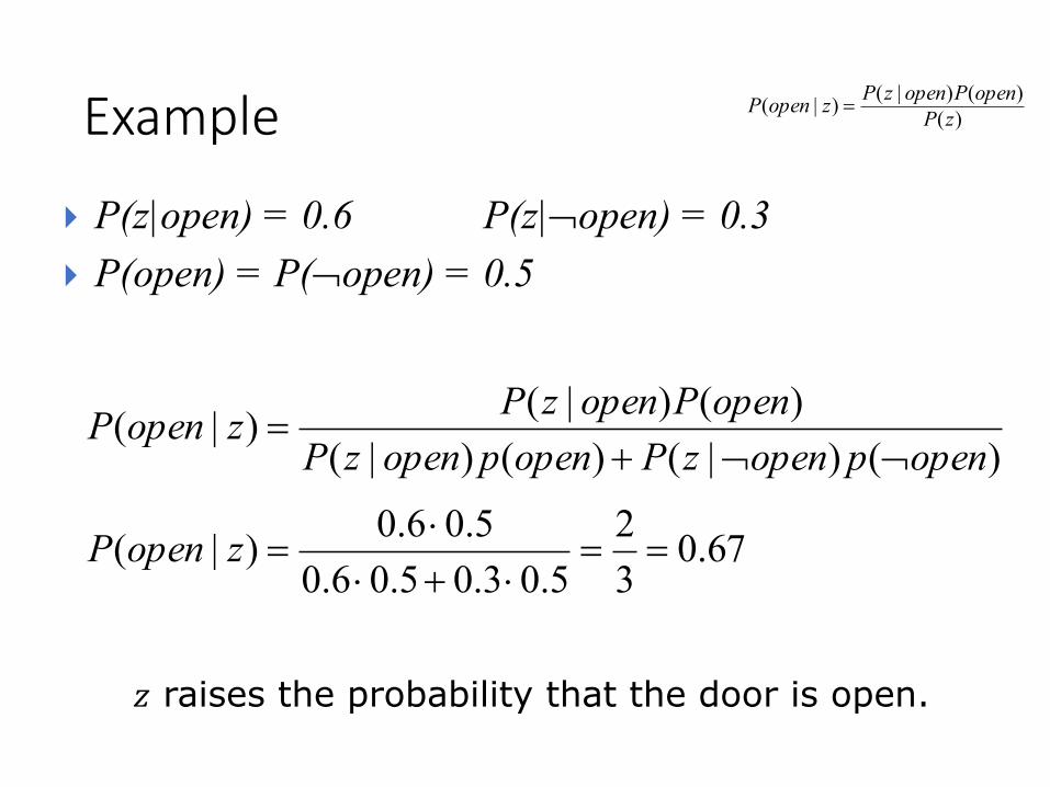
Example

} P(z|open) = 0.6 P(z|¬open) = 0.3} P(open) = P(¬open) = 0.5

67.032

5.03.05.06.05.06.0)|(

)()|()()|()()|()|(

==×+×

×=

¬¬+=

zopenP

openpopenzPopenpopenzPopenPopenzPzopenP

𝑧 raises the probability that the door is open.

)()()|()|( zP

openPopenzPzopenP =

Lets try the measurement again…

𝑃 𝑥 𝑧 = 𝜂 𝑃 𝑧 𝑥 𝑃(𝑥)

𝑃 𝑜𝑝𝑒𝑛 𝑧2 = 𝜂 𝑃 𝑧2 𝑜𝑝𝑒𝑛 𝑃(𝑜𝑝𝑒𝑛)

𝑃 𝑜𝑝𝑒𝑛 𝑧2 = 𝜂 0.6 ∗ 0.5 = 𝜂 0.3Given information:𝑃(𝑧2|𝑜𝑝𝑒𝑛) = 0.6𝑃(𝑧2|𝑐𝑙𝑜𝑠𝑒𝑑) = 0.3𝑃(𝑜𝑝𝑒𝑛) = 0.5𝑃(𝑐𝑙𝑜𝑠𝑒𝑑) = 0.5

Unlike before, we don’t yet have the answer because we still have the unknown term 𝜂 that indicates that we need to normalize to get the true probability.

𝑃 𝑐𝑙𝑜𝑠𝑒𝑑 𝑧2 = 𝜂 𝑃 𝑧2 𝑐𝑙𝑜𝑠𝑒𝑑 𝑃(𝑐𝑙𝑜𝑠𝑒𝑑)

𝑃 𝑐𝑙𝑜𝑠𝑒𝑑 𝑧2 = 𝜂 0.3 ∗ 0.5 = 𝜂 0.15

𝜂 = 0.3 + 0.15 ^2 = 2.22

𝑷 𝒐𝒑𝒆𝒏 𝒛𝟏 = 𝟎. 𝟔𝟕

Combining Evidence

• Suppose our robot obtains another observation z2. e.g. we made a second sensor reading with the same sensor, and it reports an obstacle 35cm away

• How can we integrate this new information?

• More generally, how can we estimateP(x| z1...zn )?

Generalizing the Conditionwith Bayes Theorem

𝑃 𝑥 𝑧, 𝐴𝑛𝑦𝑡ℎ𝑖𝑛𝑔 =𝑃 𝑧 𝑥, 𝐴𝑛𝑦𝑡ℎ𝑖𝑛𝑔)𝑃(𝑥|𝐴𝑛𝑦𝑡ℎ𝑖𝑛𝑔)

𝑃(𝑧|𝐴𝑛𝑦𝑡ℎ𝑖𝑛𝑔)

𝑃 𝑥 𝑧 =𝑃 𝑧 𝑥 𝑃(𝑥)

𝑃(𝑧)

In fact, we can add any arbitrary context variables on the right side of the conditioning bar, so long as we apply them in every term.

The usual version of Bayes is conditioned on a single event:

Multiple Measurements

𝑃 𝑥 𝑧, 𝐴𝑛𝑦𝑡ℎ𝑖𝑛𝑔 =𝑃 𝑧 𝑥, 𝐴𝑛𝑦𝑡ℎ𝑖𝑛𝑔)𝑃(𝑥|𝐴𝑛𝑦𝑡ℎ𝑖𝑛𝑔)

𝑃(𝑧|𝐴𝑛𝑦𝑡ℎ𝑖𝑛𝑔)

𝑃 𝑥 𝑧3, 𝐴𝑛𝑦𝑡ℎ𝑖𝑛𝑔 =𝑃 𝑧3 𝑥, 𝐴𝑛𝑦𝑡ℎ𝑖𝑛𝑔)𝑃(𝑥|𝐴𝑛𝑦𝑡ℎ𝑖𝑛𝑔)

𝑃(𝑧3|𝐴𝑛𝑦𝑡ℎ𝑖𝑛𝑔)

𝑃 𝑥 𝑧3, 𝑧2 =𝑃 𝑧3 𝑥, 𝑧2)𝑃(𝑥|𝑧2)

𝑃(𝑧3|𝑧2)

At time 𝑡 = 2, everything earlier is merely context information.

Multiple Measurements (cont)

𝑃 𝑥 𝑧3, 𝑧2 =𝑃 𝑧3 𝑥, 𝑧2)𝑃(𝑥|𝑧2)

𝑃(𝑧3|𝑧2)

At time 𝑡 = 2• 𝑃(𝑥|𝑧2) is the prior… what we believe about the state 𝑥, based on

history of measurements before 𝑡 = 2• 𝑃 𝑥 𝑧3, 𝑧2 is the posterior… what we believe about the state 𝑥,

based on history of measurements, including 𝑡 = 2• 𝑃 𝑧3 𝑥, 𝑧2) … If we really know the state 𝑥, then what we measured

at time 𝑡 = 1 won’t affect what we expect to measure at time 𝑡 = 2

Reference

• Probabilistic Robotics by Thrun, Burgard and Fox.. Chapter 2 (available on Piazza)