Embed Size (px)
Citation preview

Probability Theory
Course Notes — Harvard University — 2011
C. McMullen
May 4, 2011
Contents
I The Sample Space . . . . . . . . . . . . . . . . . . . . . . . . 2II Elements of Combinatorial Analysis . . . . . . . . . . . . . . 5III Random Walks . . . . . . . . . . . . . . . . . . . . . . . . . . 15IV Combinations of Events . . . . . . . . . . . . . . . . . . . . . 24V Conditional Probability . . . . . . . . . . . . . . . . . . . . . 29VI The Binomial and Poisson Distributions . . . . . . . . . . . . 37VII Normal Approximation . . . . . . . . . . . . . . . . . . . . . . 44VIII Unlimited Sequences of Bernoulli Trials . . . . . . . . . . . . 55IX Random Variables and Expectation . . . . . . . . . . . . . . . 60X Law of Large Numbers . . . . . . . . . . . . . . . . . . . . . . 68XI Integral–Valued Variables. Generating Functions . . . . . . . 70XIV Random Walk and Ruin Problems . . . . . . . . . . . . . . . 70I The Exponential and the Uniform Density . . . . . . . . . . . 75II Special Densities. Randomization . . . . . . . . . . . . . . . . 94
These course notes accompany Feller, An Introduction to ProbabilityTheory and Its Applications, Wiley, 1950.
I The Sample Space
Some sources and uses of randomness, and philosophical conundrums.
1. Flipped coin.
2. The interrupted game of chance (Fermat).
3. The last roll of the game in backgammon (splitting the stakes at MonteCarlo).
4. Large numbers: elections, gases, lottery.
5. True randomness? Quantum theory.
6. Randomness as a model (in reality only one thing happens). Paradox:what if a coin keeps coming up heads?
7. Statistics: testing a drug. When is an event good evidence rather thana random artifact?
8. Significance: among 1000 coins, if one comes up heads 10 times in arow, is it likely to be a 2-headed coin? Applications to economics,investment and hiring.
9. Randomness as a tool: graph theory; scheduling; internet routing.
We begin with some previews.
Coin flips. What are the chances of 10 heads in a row? The probability is1/1024, less than 0.1%. Implicit assumptions: no biases and independence.What are the chance of heads 5 out of ten times? (
(105
)= 252, so 252/1024
= 25%).
The birthday problem. What are the chances of 2 people in a crowdhaving the same birthday? Implicit assumptions: all 365 days are equallylikely; no leap days; different birthdays are independent.
Chances that no 2 people among 30 have the same birthday is about29.3%. Back of the envelope calculation gives − log P = (1/365)(1 + 2 +· · · + 29) ≈ 450/365; and exp(−450/365) = 0.291.
Where are the Sunday babies? US studies show 16% fewer births onSunday.
2

Does this make it easier or harder for people to have the same birthday?The Dean says with surprise, I’ve only scheduled 20 meetings out-of-town
for this year, and already I have a conflict. What faculty is he from?
Birthdays on Jupiter. A Jovian day is 9.925 hours, and a Jovian yearis 11.859 earth years. Thus there are N = 10, 467 possible birthdays onJupiter. How big does the class need to be to demonstrate the birthdayparadox?
It is good to know that log(2) = 0.693147 . . . ≈ 0.7. By the back ofthe envelope calculation, we want the number of people k in class to satisfy1 + 2 + . . . + k ≈ k2/2 with k2/(2N) ≈ 0.7, or k ≈
√1.4N ≈ 121.
(Although since Jupiter’s axis is only tilted 3◦, seasonal variations aremuch less and the period of one year might have less cultural significance.)
The rule of seven. The fact that 10 log(2) is about 7 is related to the‘rule of 7’ in banking: to double your money at a (low) annual interest rateof k% takes about 70/k years (not 100/k).
(A third quantity that is useful to know is log 10 ≈ π.)
The mailman paradox. A mailman delivers n letters at random to nrecipients. The probability that the first letter goes to the right person is1/n, so the probability that it doesn’t is 1− 1/n. Thus the probability thatno one gets the right letter is (1 − 1/n)n ≈ 1/e = 37%.
Now consider the case n = 2. Then he either delivers the letters for Aand B in order (A,B) or (B,A). So there is a 50% chance that no one getsthe right letter. But according to our formula, there is only a 25% chancethat no one gets the right letter.
What is going on?
Outcomes; functions and injective functions. The porter’s deliveriesare described by the set S of all functions f : L → B from n letters to nboxes. The mailman’s deliveries are described by the space S′ ⊂ S of all1 − 1 functions f : L → B. We have |S| = nn and |S′| = n!; they givedifferent statistics for equal weights.
The sample space. The collection S of all possible completely specifiedoutcomes of an experiment or task or process is called the sample space.
Examples.
1. For a single toss at a dartboard, S is the unit disk.
2. For the high temperature today, S = [−50, 200].
3. For a toss of a coin, S = {H,T}.
3
4. For the roll of a die, S = {1, 2, 3, 4, 5, 6}.
5. For the roll of two dice, |S| = 36.
6. For n rolls of a die, S = {(a1, . . . , an) : 1 ≤ ai ≤ 6}; we have |S| = 6n.More formally, S is the set of functions on [1, 2, . . . , n] with values in[1, 2, . . . , 6].
7. For shuffling cards, |S| = 52! = 8 × 1067.
An event is a subset of S. For example: a bull’s eye; a comfortable day;heads; an odd number on the die; dice adding up to 7; never getting a 3 inn rolls; the first five cards form a royal flush.
Logical combinations of events correspond to the operators of set theory.For example:
A′ = not A = S − A; A ∩ B = A and B; A ∪ B = A or B.
Probability. We now focus attention on a discrete sample space. Thena probability measure is a function p : S → [0, 1] such that
∑S p(s) = 1.
Often, out of ignorance or because of symmetry, we have p(s) = 1/|S| (allsamples have equal likelihood).
The probability of an event is given by
P (A) =∑
s∈A
p(s).
If all s have the same probability, then P (A) = |A|/|S|.
Proposition I.1 We have P (A′) = 1 − P (A).
Note that this formula is not based on intuition (although it coincideswith it), but is derived from the definitions, since we have P (A) + P (A′) =P (S) = 1. (We will later treat other logical combinations of events).
Example: mail delivery. The pesky porter throws letters into the pi-geonholes of the n students; S is the set of all functions f : n → n. Whilethe mixed-up mailman simple chooses a letter at random for each house; Sis the space of all bijective functions f : n → n. These give different answersfor the probability of a successful delivery. (Exercise: who does a better jobfor n = 3? The mailman is more likely than the porter to be a completefailure — that is, to make no correct delivery. The probability of failure forthe porter is (2/3)3 = 8/27, while for the mailman it is 1/3 = 2/3! = 8/24.
4

This trend continues for all n, although for both the probability of completefailure tends to 1/e.)
An infinite sample space. Suppose you flip a fair coin until it comesup heads. Then S = N ∪ {∞} is the number of flips it takes. We havep(1) = 1/2, p(2) = 1/4, and
∑∞n=1 1/2n = 1, so p(∞) = 0.
The average number of flips it takes is E =∑∞
1 n/2n = 2. To evaluatethis, we note that f(x) =
∑∞1 xn/2n = (x/2)/(1 − x/2) satisfies f ′(x) =∑∞
1 nxn−1/2n and hence E = f ′(1) = 2. This is the method of generatingfunctions.
Benford’s law. The event that a number X begins with a 1 in base 10depends only on log(X)mod 1 ∈ [0, 1]. It occurs when log(X) ∈ [0, log 2] =[0, 0.30103 . . .]. In some settings (e.g. populations of cities, values of theDow) this means there is a 30% chance the first digit is one (and only a 5%chance that the first digit is 9).
For example, once the Dow has reached 1,000, it must double in value tochange the first digit; but when it reaches 9,000, it need only increase about10% to get back to one.
II Elements of Combinatorial Analysis
Basic counting functions.
1. To choose k ordered items from a set A, with replacement, is thesame as to choose an element of Ak. We have |Ak| = |A|k. Similarly|A × B × C| = |A| · |B| · |C|.
2. The number of maps f : A → B is |B||A|.
3. The number of ways to put the elements of A in order is the same asthe number of bijective maps f : A → A. It is given by |A|!.
4. The number of ways to choose k different elements of A in order,a1, . . . , ak, is
(n)k = n(n − 1) · · · (n − k + 1) =n!
(n − k)!,
where n = |A|.
5. The number of injective maps f : B → A is (n)k where k = |B| andn = |A|.
5

6. The subsets P(A) of A are the same as the maps f : A → 2. Thus|P(A)| = 2|A|.
7. Binomial coefficients. The number of k element subsets of A is givenby (
n
k
)=
n!
k!(n − k)!=
(n)kk!
·
This second formula has a natural meaning: it is the number of orderedsets with k different elements, divided by the number of orderings ofa given set. It is the most efficient method for computation. Also it isremarkable that this number is an integer; it can always be computedby cancellation. E.g.
(10
5
)=
10 · 9 · 8 · 7 · 65 · 4 · 3 · 2 · 1 =
10
2 · 5 · 9
3· 8
4· 7 · 6 = 6 · 42 = 252.
8. These binomial coefficients appear in the formula
(a + b)n =
n∑
0
(n
k
)akbn−k.
Setting a = b = 1 shows that |P(A)| is the sum of the number ofk-element subsets of A for 0 ≤ k ≤ n.
From the point of view of group theory, Sn acts transitively on thek-element subsets of A, with the stabilizer of a particular subset iso-morphic to Sk × Sn−k.
9. The number of ways to assign n people to teams of size k1, . . . , ks with∑ki = n is (
n
k1 k2 · · · ks
)=
n!
k1! · · · ks!·
Walks on a chessboard. The number of shortest walks that start at onecorner and end at the opposite corner is
(147
).
Birthdays revisited. The number of possible birthdays for k people is365k, while the number of possible distinct birthdays is (365)k . So theprobability that no matching birthdays occur is
p =(365)k365k
=k!
365k
(365
k
)·
6
Senators on a committee. The probability p that Idaho is representedon a committee of 50 senators satisfies
1 − p = q =
(98
50
)/(100
50
)=
50 · 49100 · 99 = 0.247475.
So there is more than a 3/4 chance. Why is it more than 3/4? If there firstsenator is not on the committee, then the chance that the second one is risesto 50/99. So
p = 1/2 + 1/2(50/99) = 0.752525 . . .
(This is an example of conditional probabilities.) Note that this calculationis much simpler than the calculation of
(10050
), a 30 digit number.
The probability that all states are represented is
p = 250
/(100
50
)≈ 1.11 × 10⁻¹⁴.
Poker. The number of poker hands is(525
), about 2.5 million. Of these,
only 4 give a royal flush. The odds of being dealt a royal flush are worsethan 600,000 to one.
The probability p of a flush can be found by noting that there are(13
5
)
hands that are all spades; thus
p = 4
(13
5
)/(52
5
)=
33
16660= 0.198%.
Note that some of these flushes may have higher values, e.g. a royal flush isincluded in the count above.
The probability p of just a pair (not two pair, or three of a kind, or afull house) is also not too hard to compute. There are 13 possible valuesfor the pair. The pair also determines 2 suits, which can have
(42
)possible
values. The remaining cards must represent different values, so there are(123
)choices for them. Once they are put in numerical order, they give a list
of 3 suits, with 43 possibilities. Thus the number of hands with just a pairis
N = 13
(4
2
)(12
3
)43 = 1, 098, 240,
and the probability is p = N/(525
)which gives about 42%. There is almost
a 50% chance of having at least a pair.
Bridge. The number of bridge hands, N =(5213
), is more than half a trillion.
The probability of a perfect hand (all one suit) is 4/N , or about 158 billion
7

to one. A typical report of such an occurrence appears in the Sharon Herald(Pennsylvania), 16 August 2010. Is this plausible? (Inadequate shufflingmay play a role.) Note: to win with such a hand, you still need to win thebidding and have the lead.
There are 263,333 royal flushes for every perfect hand of bridge.
Flags. The number of ways to fly k flags on n poles (where the verticalorder of the flags matters) is N = n(n + 1) · · · (n + k − 1). This is becausethere are n positions for the first flag but n + 1 for the second, because itcan go above or below the first.
If the flags all have the same color, there are
N
k!=
(n + k − 1
k
)=
(n + k − 1
n − 1
)
arrangements. This is the same as the number of monomials of degree k inn variables. One can imagine choosing n − 1 moments for transition in aproduct of k elements. Until the first divider is reached, the terms in theproduct represent the variable x1; then x2; etc.
Three types of occupation statistics. There are three types of commonsample spaces or models for k particles occupying n states, or k balls drop-ping into n urns, etc. In all these examples, points in the sample space haveequal probability; but the sample spaces are different.
Maxwell–Boltzmann statistics. The balls are numbered 1, . . . k and thesample space is the set of sequences (a1, . . . , ak) with 1 ≤ ai ≤ n. Thus S isthe set of maps f : k → n. With n = 365, this is used to model to birthdaysoccurring in class of size k.
Bose–Einstein statistics. The balls are indistinguishable. Thus the sam-ple space is just the number of balls in each urn: the set of (k1, . . . , kn) suchthat
∑ki = k. Equivalently S is the quotient of the set of maps f : k → n
by the action of Sk.Fermi–Dirac statistics. No more than one ball can occupy a given urn,
and the balls are indistinguishable. Thus the sample space S is just thecollection of subsets A ⊂ n such that |A| = k; it satisfies |S| =
(nk
).
Indistinguishable particles: Bosons. How many ways can k identicalparticles occupy n different cells (e.g. energy levels)? This is the same asflying identical flags; the number of ways is the number of solutions to
k1 + · · · + kn = k
with ki ≥ 0, and is given by(n+k−1
k
)as we have seen.
8
In physics, k photons arrange themselves so all such configurations areequally likely. For example, when n = k = 2 the arrangements 2 + 0, 1 + 1and 0 + 2 each have probability 1/3. This is called Bose–Einstein statistics.
This is different from Maxwell-Boltzmann statistics, which are modeledon assigning 2 photons, one at a time, to 2 energy levels. In the lattercase 1+1 has probability 1/2. Particles like photons (called bosons) cannotbe distinguished from one another, so this partition counts as only one casephysically (it does not make sense to say ‘the first photon went in the secondslot’).
Example: Runs. If we require that every cell is occupied, i.e. if we requirethat ki ≥ 1 for all i, then the number of arrangements is smaller: it is givenby
N =
(k − 1
k − n
)·
Indeed, we can ‘prefill’ each of the n states with a single particle; then wemust add to this a distribution of k−n particles by the same rule as above.
As an example, when 5 people sit at a counter of 16 seats, the n runsof free and occupied seats determine a partition k = 16 = k1 + · · · + kn.The pattern EOEEOEEEOEEEOEOE, for example, corresponds to 16 =1 + 1 + 2 + 1 + 3 + 1 + 3 + 1 + 1 + 1 + 1. Here n = 11, that is, there are 11runs (the maximum possible).
Is this evidence that diners like to have spaces between them? Thenumber of possible seating arrangements is
(165
). That is, our sample space
consists of injective maps from people to seats (Fermi–Dirac statistics). Toget 11 runs, each diner must have an empty seat to his right and left. Thusthe number of arrangements is the same as the number of partitions of theremaining k = 11 seats into 6 runs with k1 + · · · + k6 = 11. Since eachki ≥ 1, this can be done in
(105
)ways (Bose–Einstein statistics). Thus the
probability of 11 runs arising by chance is
p =
(10
5
)/(16
5
)= 3/52 = 0.0577 . . .
Misprints and exclusive particles: Fermions. Electrons, unlike pho-tons, obey Fermi–Dirac statistics: no two can occupy the same state (by thePauli exclusion principle). Thus the number of ways k particles can occupyn states is
(nk
). For example, 1 + 1 is the only distribution possible for 2
electrons in 2 states. In Fermi–Dirac statistics, these distributions are allgiven equal weight.
9
When a book of length n has k misprints, these must occur in distinctpositions, so misprints are sometimes modeled on fermions.
Samples: the hypergeometric distribution. Suppose there are A de-fects among N items. We sample n items. What is the probability of findinga defects? It’s given by:
pa =
(n
a
)(N − n
A − a
)/(N
A
)·
(Imagine the N items in order; mark A at random as defective, and thensample the first n.) Note that
∑pa = 1.
We have already seen a few instances of it: for example, the probabilitythat a sample of 2 senators includes none from a committee of 50 is the casen = 2, N = 100, A = 50 and a = 0. The probability of 3 aces in a hand ofbridge is
p3 =
(13
3
)(39
1
)/(52
4
)≈ 4%,
while the probability of no aces at all is
p0 =
(13
0
)(39
4
)/(52
4
)≈ 30%.
Single samples. The simple identity
(N − 1
A − 1
)=
A
N
(N
A
)
shows that p1 = A/N . The density of defects in the total population givesthe probability that any single sample is defective.
Symmetry. We note that pa remains the same if the roles of A and nare interchanged. Indeed, we can imagine choosing 2 subsets of N , withcardinalities A and n, and then asking for the probability pa that theiroverlap is a. This is given by the equivalent formula
pa =
(N
a
)(N − a
n − a,A − a
)/(N
n
)(N
A
),
which is visibly symmetric in (A,n) and can be simplified to give the formulaabove. (Here
(ab,c
)= a!/(b!c!(a − b − c)!) is the number of ways of choosing
disjoint sets of size b and c from a universe of size a.) Here is the calculation
10
showing agreement with the old formula. We can drop(NA
)from both sides.
Then we find:
(N
a
)(N − a
n − a,A − a
)(N
n
)−1
=N !(N − a)!n!(N − n)!
a!(N − a)!(n − a)!(A − a)!(N − n − A + a)!N !
=n!(N − n)!
(n − a)!a!(A − a)!(N − n − A + a)!=
(n
a
)(N − n
A − a
),
as desired.
Limiting case. If N and A go to infinity with A/N = p fixed, and n, afixed, then we find
pa →(
n
a
)pa(1 − p)n−a.
This is intuitively justified by the idea that in a large population, each of nsamples independently has a chance A/N of being defective. We will laterstudy in detail this important binomial distribution.
To see this rigorously we use a variant of the previous identity:
(N − 1
A
)=
(N − 1
N − A − 1
)=
(1 − A
N
)(N
A
)·
We already know (N − a
A − a
)≈(
A
N
)a(N
A
),
and the identity above implies
(N − n
A − a
)≈(
1 − A
N
)n−a(N − a
A − a
).
This yields the desired result.
Statistics and fish. The hypergeometric distribution is important instatistics: a typical problem there is to give a confident upper bound forA based solely on a.
In Lake Champlain, 1000 fish are caught and marked red. The next dayanother 1000 fish are caught and it is found that 50 are red. How many fishare in the lake?
Here we know n = 1000, a = 50 and A = 1000, but we don’t know N . Tomake a guess we look at the value of N ≥ 1950 which makes p50 as large aspossible — this is the maximum likelihood estimator. The value N = 1950is very unlikely — it means all fish not captured are red. A very large value
11

of N is also unlikely. In fact pa(N) first increases and then decreases, as canbe seen by computing
pa(N)
pa(N − 1)=
(N − n)(N − A)
(N − n + a − A)N·
(The formula looks nicer with N − 1 on the bottom than with N + 1 onthe top.) This fraction is 1 when a/n = A/N . So we estimate A/N by50/1000 = 1/20, and get N = 20A = 20, 000.
Waiting times. A roulette table with n slots is spun until a given luckynumber — say 7 — come up. What is the probability pk that this takesmore than k spins?
There are nk possible spins and (n − 1)k which avoid the number 7. So
pk =
(1 − 1
n
)k
.
This number decreases with k. The median number of spins, m, arises whenpk ≈ 1/2; half the time it takes longer than m (maybe much longer), halfthe time shorter. If n is large then we have the approximation
log 2 = log(1/pm) = m/n
and hence m ≈ n log 2. So for 36 slots, a median of 25.2 spins is expected.(In a real roulette table, there are 38 slots, which include 0 and 00 for thehouse; the payoff would only be fair if there were 36 slots.)
Similarly, if we are waiting for a student to arrive with the same birthdayas Lincoln, the median waiting time is 365 log 2 = 255 students.
Expected value. In general if X : S → R is a real-valued function, wedefine its average or expected value by
E(X) =∑
S
p(s)X(s).
We can also rewrite this as
E(X) =∑
t
tP (X = t),
where t ranges over the possible values of X. This is the weighted averageof X, so it satisfies min X(s) ≤ E(X) ≤ max X(s). Note also that E(X)need not be a possible value of X. For example, if X assumes the values 0and 1 for a coin flip, then E(X) = 1/2.
12
1
1
p2
q3
p3
q2
q1
0
p
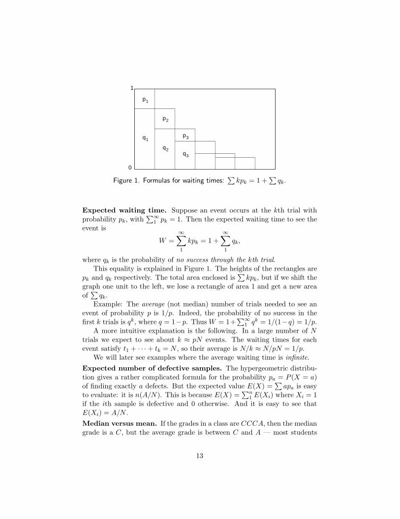
Figure 1. Formulas for waiting times:∑
kpk = 1 +∑
qk.
Expected waiting time. Suppose an event occurs at the kth trial withprobability pk, with
∑∞1 pk = 1. Then the expected waiting time to see the
event is
W =∞∑
1
kpk = 1 +∞∑
1
qk,
where qk is the probability of no success through the kth trial.This equality is explained in Figure 1. The heights of the rectangles are
pk and qk respectively. The total area enclosed is∑
kpk, but if we shift thegraph one unit to the left, we lose a rectangle of area 1 and get a new areaof∑
qk.Example: The average (not median) number of trials needed to see an
event of probability p is 1/p. Indeed, the probability of no success in thefirst k trials is qk, where q = 1−p. Thus W = 1+
∑∞1 qk = 1/(1−q) = 1/p.
A more intuitive explanation is the following. In a large number of Ntrials we expect to see about k ≈ pN events. The waiting times for eachevent satisfy t1 + · · · + tk = N , so their average is N/k ≈ N/pN = 1/p.
We will later see examples where the average waiting time is infinite.
Expected number of defective samples. The hypergeometric distribu-tion gives a rather complicated formula for the probability pa = P (X = a)of finding exactly a defects. But the expected value E(X) =
∑apa is easy
to evaluate: it is n(A/N). This is because E(X) =∑n
1 E(Xi) where Xi = 1if the ith sample is defective and 0 otherwise. And it is easy to see thatE(Xi) = A/N .
Median versus mean. If the grades in a class are CCCA, then the mediangrade is a C, but the average grade is between C and A — most students
13
are below average.
Stirling’s formula. For smallish values of n, one can find n! by hand, ina table or by computer, but what about for large values of n? For example,what is 1,000,000!?
Theorem II.1 (Stirling’s formula) For n → ∞, we have
n! ∼√
2πn(n/e)n =√
2πnn+1/2e−n,
meaning the ratio of these two quantities tends to one.
Sketch of the proof. Let us first estimate L(n) = log(n!) =∑n
1 log(k) byan integral. Since (x log x − x)′ = log x, we have
L(n) ≈∫ n+1
1log x dx = (n + 1) log(n + 1) − n.
In fact rectangles of total area L(n) fit under this integral with room tospare; we can also fit half-rectangles of total area about (log n)/2. Theremaining error is bounded and in fact tends to a constant; this gives
L(n) = (n + 1/2) log n − n + C + o(1),
which gives n! ∼ eCnn+1/2e−n for some C. The value of C will be determinedin a natural way later, when we discuss the binomial distribution.
Note we have used the fact that limn→∞ log(n + 1) − log(n) = 0.
Appendix: Some calculus facts. In the above we have used some ele-mentary facts from algebra and calculus such as:
n(n + 1)
2= 1 + 2 + · · · + n,
ex = 1 + x +x2
2!+ · · · =
∞∑
0
xn
n!,
ex = limn→∞
(1 +
x
n
),
log(1 + x) = x − x2/2 + x3/3 − · · · =
∞∑
1
(−1)n+1xn/n.
This last follows from the important formula
1 + x + x2 + · · · =1
1 − x,
14

which holds for |x| < 1. These formulas are frequent used in the form
(1 − p) ≈ e−p and log(1 − p) ≈ −p,
which are valid when p is small (the error is of size O(p2). Special cases ofthe formula for ex are (1 + 1/n)n → e and (1 − 1/n)n → 1/e. We also have
log 2 = 1 − 1/2 + 1/3 − 1/4 + · · · = 0.6931471806 . . . ,
and ∫log x dx = x log x − x + C.
III Random Walks
One of key ideas in probability is to study not just events but processes,which evolve in time and are driven by forces with a random element.
The prototypical example of such a process is a random walk on theintegers Z.
Random walks. By a random walk of length n we mean a sequence ofintegers (s0, . . . , sn) such that s0 = 0 and |si − si−1| = 1. The number ofsuch walks is N = 2n and we give all walks equal probability 1/2n. Youcan imagine taking such a walk by flipping a coin at each step, to decidewhether to move forward or backward.
Expected distance. We can write sn =∑n
1 xi, where each xi = ±1. Thenthe expected distance squared from the origin is:
E(s2n) = E
(∑x2
i
)+∑
i6=j
E(xixj) = n.
This yields the key insight that after n steps, one has generally wanderedno more than distance about
√n from the origin.
Counting walks. The random walk ends at a point x = sn. We alwayshave x ∈ [−n, n] and x = n mod2. It is usual to think of the random walkas a graph through the points (0, 0), (1, s1), . . . (n, sn) = (n, x).
It is useful to write
n = p + q and x = p − q.
(That is, p = (n+x)/2 and q = (n−x)/2.) Suppose x = p−q and n = p+q.Then in the course of the walk we took p positive steps and q negative steps.
15

To describe the walk, which just need to choose which steps are positive.Thus the number of walks from (0, 0) to (n, x) is given by
Nn,x =
(p + q
p
)=
(p + q
q
)=
(n
(n + x)/2
)=
(n
(n − x)/2
)·
In particular, the number of random walks that return to the origin in 2nsteps is given by
N2n,0 =
(2n
n
)·
Coin flips. We can think of a random walks as a record of n flips of a coin,and sk as the difference between the number of heads and tails seen so far.Thus px = Nn,x/2n is the probability of x more heads than tails, and N2n,0
is the probability of seeing exactly half heads, half tails in 2n flips.We will later see that for fixed n, N2n,x approximates a bell curve, and
N2n,0 is the highest point on the curve.
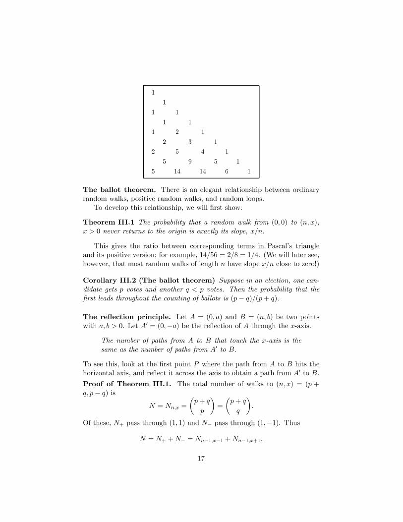
Pascal’s triangle. The number of paths from (0, 0) to (n, k) is just thesum of the number of paths to (n−1, k−1) and (n−1, k+1). This explainsPascal’s triangle; the table of binomial coefficients is the table of the valuesof Nn,x, with x horizontal and n increasing down the page.
1
1 1
1 2 1
1 3 3 1
1 4 6 4 1
1 5 10 10 5 1
1 6 15 20 15 6 1
1 7 21 35 35 21 7 1
1 8 28 56 70 56 28 8 1
We can also consider walks which begin at 0, and possibly end at 0, butwhich must otherwise stay on the positive part of the axis. The number ofsuch paths Pn,x which end at x after n steps can also be computed recursivelyby ignoring the entries in the first column when computing the next row.Here we have only shown the columns x ≥ 0.
16
1
1
1 1
1 1
1 2 1
2 3 1
2 5 4 1
5 9 5 1
5 14 14 6 1
The ballot theorem. There is an elegant relationship between ordinaryrandom walks, positive random walks, and random loops.
To develop this relationship, we will first show:
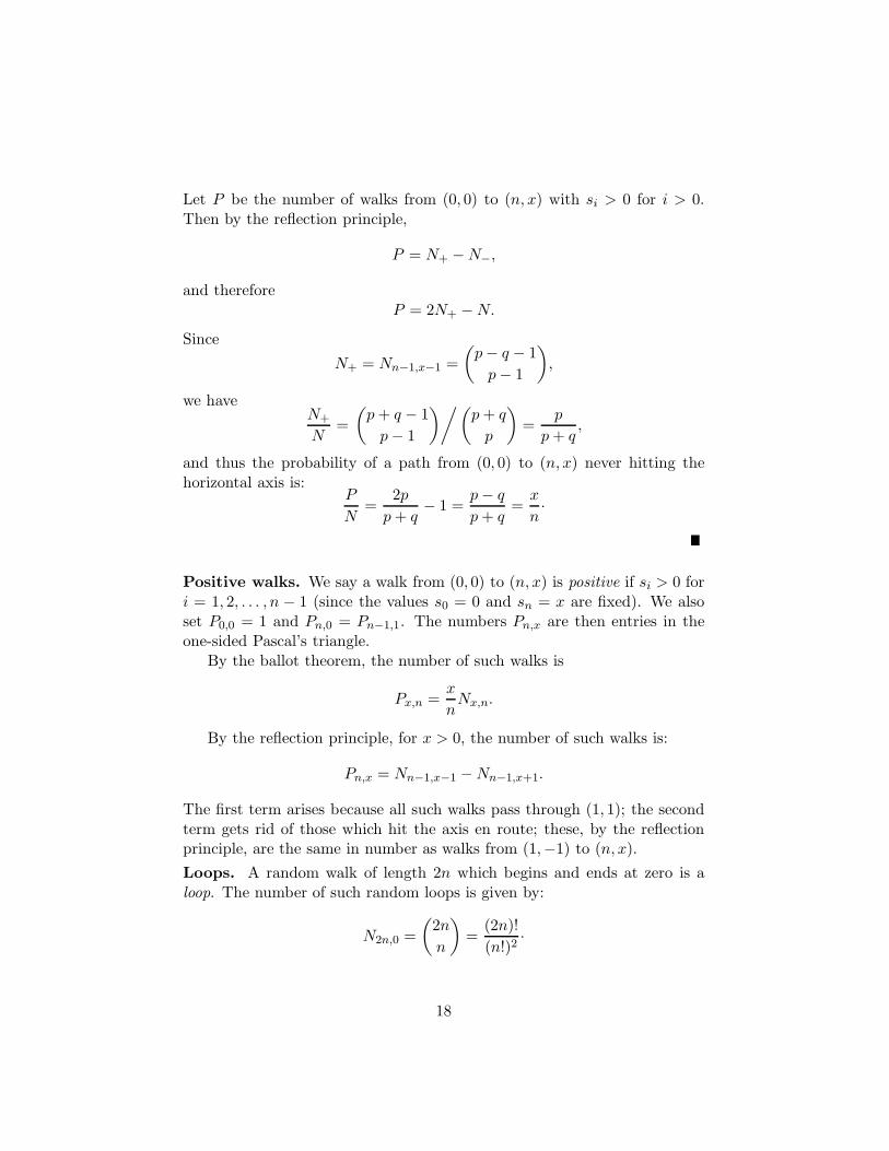
Theorem III.1 The probability that a random walk from (0, 0) to (n, x),x > 0 never returns to the origin is exactly its slope, x/n.
This gives the ratio between corresponding terms in Pascal’s triangleand its positive version; for example, 14/56 = 2/8 = 1/4. (We will later see,however, that most random walks of length n have slope x/n close to zero!)
Corollary III.2 (The ballot theorem) Suppose in an election, one can-didate gets p votes and another q < p votes. Then the probability that thefirst leads throughout the counting of ballots is (p − q)/(p + q).
The reflection principle. Let A = (0, a) and B = (n, b) be two pointswith a, b > 0. Let A′ = (0,−a) be the reflection of A through the x-axis.
The number of paths from A to B that touch the x-axis is thesame as the number of paths from A′ to B.
To see this, look at the first point P where the path from A to B hits thehorizontal axis, and reflect it across the axis to obtain a path from A′ to B.
Proof of Theorem III.1. The total number of walks to (n, x) = (p +q, p − q) is
N = Nn,x =
(p + q
p
)=
(p + q
q
).
Of these, N+ pass through (1, 1) and N− pass through (1,−1). Thus
N = N+ + N− = Nn−1,x−1 + Nn−1,x+1.
17
Let P be the number of walks from (0, 0) to (n, x) with si > 0 for i > 0.Then by the reflection principle,
P = N+ − N−,
and thereforeP = 2N+ − N.
Since
N+ = Nn−1,x−1 =
(p − q − 1
p − 1
),
we haveN+
N=
(p + q − 1
p − 1
)/(p + q
p
)=
p
p + q,
and thus the probability of a path from (0, 0) to (n, x) never hitting thehorizontal axis is:
P
N=
2p
p + q− 1 =
p − q
p + q=
x
n·
Positive walks. We say a walk from (0, 0) to (n, x) is positive if si > 0 fori = 1, 2, . . . , n − 1 (since the values s0 = 0 and sn = x are fixed). We alsoset P0,0 = 1 and Pn,0 = Pn−1,1. The numbers Pn,x are then entries in theone-sided Pascal’s triangle.
By the ballot theorem, the number of such walks is
Px,n =x
nNx,n.
By the reflection principle, for x > 0, the number of such walks is:
Pn,x = Nn−1,x−1 − Nn−1,x+1.
The first term arises because all such walks pass through (1, 1); the secondterm gets rid of those which hit the axis en route; these, by the reflectionprinciple, are the same in number as walks from (1,−1) to (n, x).
Loops. A random walk of length 2n which begins and ends at zero is aloop. The number of such random loops is given by:
N2n,0 =
(2n
n
)=
(2n)!
(n!)2·
18
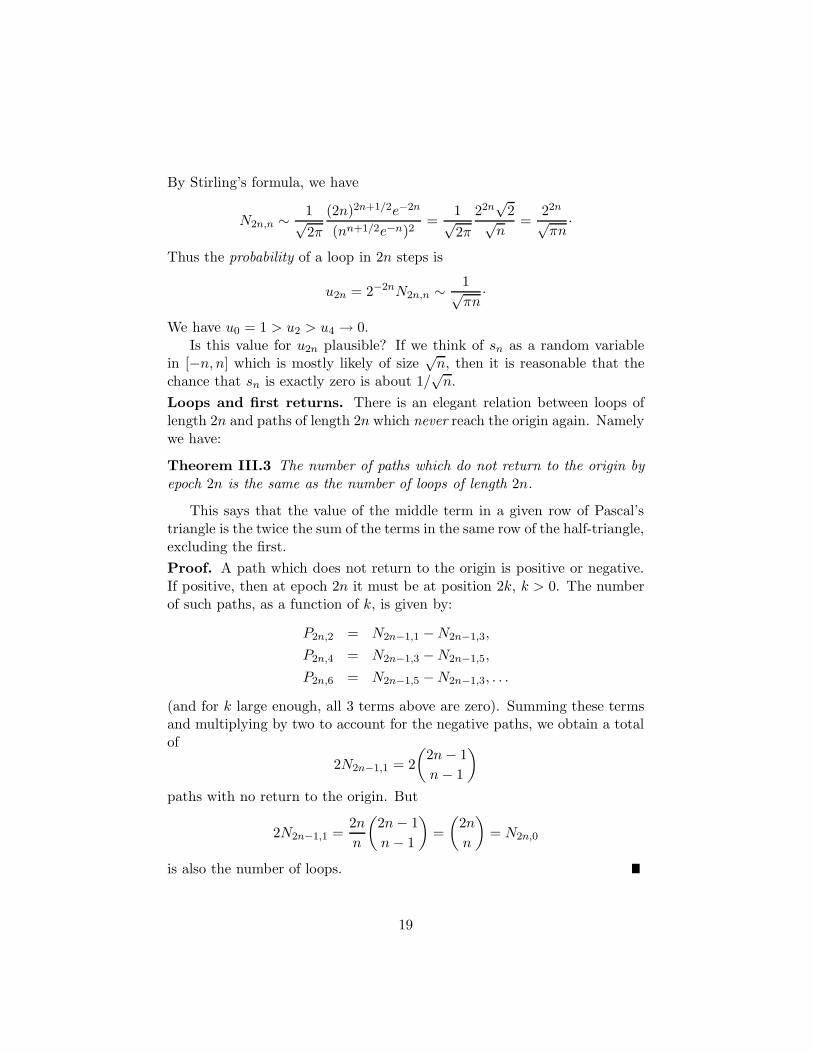
By Stirling’s formula, we have
N2n,n ∼ 1√2π
(2n)2n+1/2e−2n
(nn+1/2e−n)2=
1√2π
22n√
2√n
=22n
√πn
·
Thus the probability of a loop in 2n steps is
u2n = 2−2nN2n,n ∼ 1√πn
·
We have u0 = 1 > u2 > u4 → 0.Is this value for u2n plausible? If we think of sn as a random variable
in [−n, n] which is mostly likely of size√
n, then it is reasonable that thechance that sn is exactly zero is about 1/
√n.
Loops and first returns. There is an elegant relation between loops oflength 2n and paths of length 2n which never reach the origin again. Namelywe have:
Theorem III.3 The number of paths which do not return to the origin byepoch 2n is the same as the number of loops of length 2n.
This says that the value of the middle term in a given row of Pascal’striangle is the twice the sum of the terms in the same row of the half-triangle,excluding the first.
Proof. A path which does not return to the origin is positive or negative.If positive, then at epoch 2n it must be at position 2k, k > 0. The numberof such paths, as a function of k, is given by:
P2n,2 = N2n−1,1 − N2n−1,3,
P2n,4 = N2n−1,3 − N2n−1,5,
P2n,6 = N2n−1,5 − N2n−1,3, . . .
(and for k large enough, all 3 terms above are zero). Summing these termsand multiplying by two to account for the negative paths, we obtain a totalof
2N2n−1,1 = 2
(2n − 1
n − 1
)
paths with no return to the origin. But
2N2n−1,1 =2n
n
(2n − 1
n − 1
)=
(2n
n
)= N2n,0
is also the number of loops.
19
Event matching proofs. This last equality is also clear from the perspec-tive of paths: loops of length 2n are the same in number as walks of onestep less with s2n−1 = ±1.
The equality of counts suggests there should be a geometric way to turn apath with no return into a loop, and vice-versa. See Feller, Exercise III.10.7(the argument is due to Nelson).
Corollary III.4 The probability that the first return to the origin occurs atepoch 2n is:
f2n = u2n−2 − u2n.
Proof. The set of walks with first return at epoch 2n is contained in theset of those with no return through epoch 2n − 2; with this set, we mustexclude those with no return through epoch 2n.
Ballots and first returns. The ballot theorem also allows us to computeF2n, the number of paths which make a first return to the origin at epoch2n; namely, we have:
F2n =1
2n − 1
(2n
n
).
To see this, note that F2n is number of walks which arrive at ±1 in 2n − 1steps without first returning to zero. Thus it is twice the number whicharrive at 1. By the ballot theorem, this gives
F2n =2
2n − 1
(2n − 1
n − 1
)=
1
2n − 1
2n
n
(2n − 1
n − 1
)=
1
2n − 1
(2n
n
).
This gives
f2n = 2−2nF2n =u2n
2n − 1.
Recurrence behavior. The probability u2n of no return goes to zero like1/√
n; thus we have shown:
Theorem III.5 With probability one, every random walk returns to theorigin infinitely often.
How long do we need to wait until the random walk returns? We haveu2 = 1/2 so the median waiting time is 2 steps.
20
What about the average value of n > 0 such that s2n = 0 for the firsttime? This average waiting time is 1+ the probability u2n of failing to returnby epoch 2n; thus it is given by
T = 1 +∞∑
1
u2n ∼ 1 +∑ 1√
πn= ∞.
Thus the returns to the origin can take a long time!
Equalization of coin flips. If we think in terms of flipping a coin, wesay there is equalization at flip 2n if the number of heads and tails seenso far agree at that point. As one might expect, there are infinitely manyequalizations, and already there is a 50% chance of seeing one on the 2ndflip. But the probability of no equalization in the first 100 flips is
u100 ≈ 1√50π
= 0.0797885 . . . ,
i.e. this event occurs about once in every 12 trials.
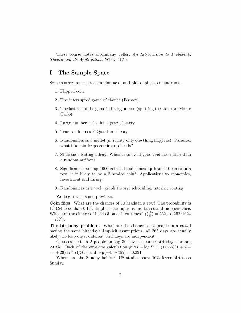
0.0 0.2 0.4 0.6 0.8 1.0
0.5
1.0
1.5
2.0
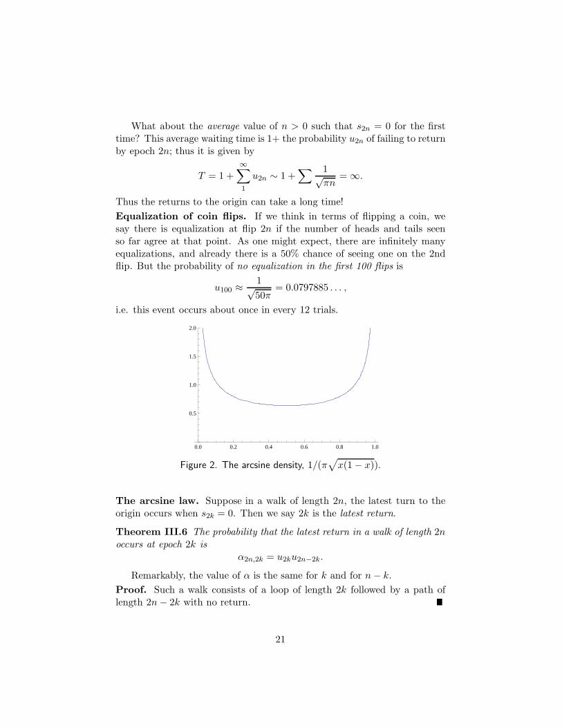
Figure 2. The arcsine density, 1/(π√
x(1 − x)).
The arcsine law. Suppose in a walk of length 2n, the latest turn to theorigin occurs when s2k = 0. Then we say 2k is the latest return.
Theorem III.6 The probability that the latest return in a walk of length 2noccurs at epoch 2k is
α2n,2k = u2ku2n−2k.
Remarkably, the value of α is the same for k and for n − k.
Proof. Such a walk consists of a loop of length 2k followed by a path oflength 2n − 2k with no return.
21
200 400 600 800 1000
-20
-10
10
20
30
200 400 600 800 1000
-30
-20
-10
10
200 400 600 800 1000
-40
-30
-20
-10
200 400 600 800 1000
-50
-40
-30
-20
-10
200 400 600 800 1000
-60
-50
-40
-30
-20
-10
10
200 400 600 800 1000
-20
-10
10
20
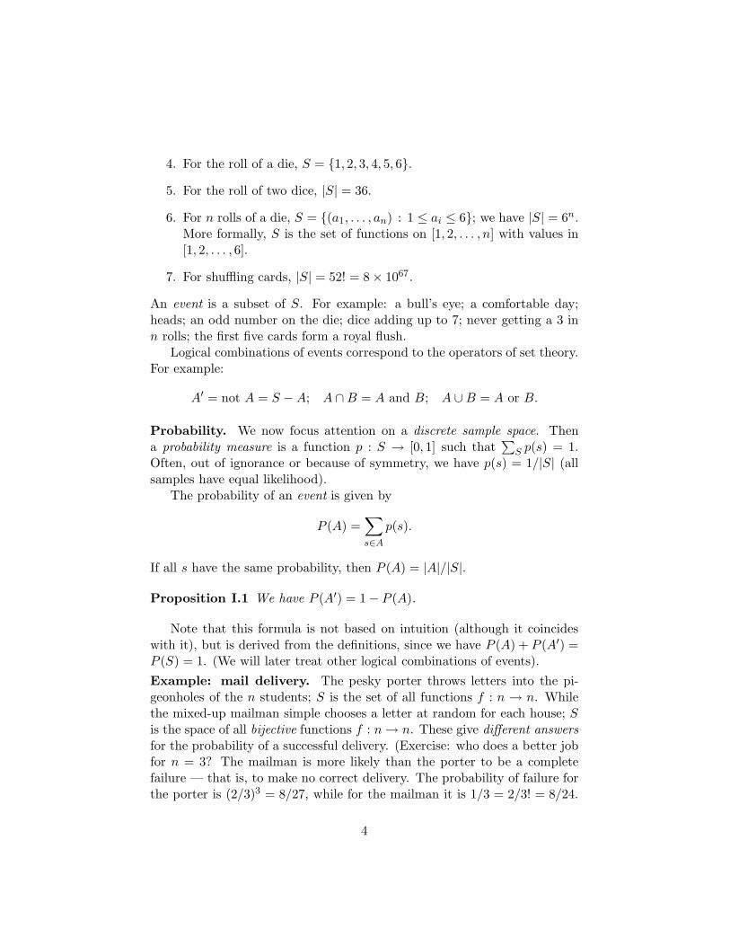
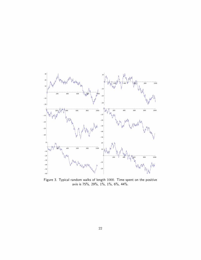
Figure 3. Typical random walks of length 1000. Time spent on the positive
axis is 75%, 29%, 1%, 1%, 6%, 44%.
22
We already know that u2k ∼ 1/√
πk, and thus
α2n,2nx ∼ 1
n
1
π√
x(1 − x)·
Consequently, we have:
Theorem III.7 As n → ∞, the probability that the last return to the originin a walk of length n occurs before epoch nx converges to
∫ x
0
dt
π√
t(1 − t)=
2
πarcsin
√x.
Proof. The probability of last return before epoch nx is
nx∑
k=0
α2n,2k =
nx∑
k=0
α2n,2n(k/n) ∼nx∑
k=0
F (k/n) (1/n) →∫ x
0F (t) dt,
where F (x) = 1/(π√
x(1 − x)).
Remark. Geometrically, the arcsine density dx/(π√
x(1 − x)) on [0, 1]gives the distribution of the projection to [0, 1] of a random point on thecircle of radius 1/2 centered at (1/2, 0).
By similar reasoning one can show:
Theorem III.8 The percentage of time a random walk spends on the posi-tive axis is also distributed according to the arcsine law.
More precisely, the probability b2k,2n of spending exactly time 2k withx > 0 in a walk of length 2n is also u2ku2n−2k. Here the random walk istaken to be piecewise linear, so it spends no time at the origin. See Figure 3for examples. Note especially that the amount of time spent on the positiveaxis does not tend to 50% as n → ∞.
Sketch of the proof. The proof is by induction. One considers walkswith 1 ≤ k ≤ n − 1 positive sides; then there must be a first return to theorigin at some epoch 2r, 0 < 2r < 2n. This return gives a loop of length 2rfollowed by a path of walk of length 2n−2r with either 2k or 2k−2r positivesides. We thus get a recursive formula for b2k,2n allowing the theorem to beverified.
23
IV Combinations of Events
We now return to the general discussion of probability theory. In this sectionand the next we will focus on the relations that hold between the probabil-ities of 2 or more events. This considerations will give us additional com-binatorial tools and lead us to the notions of conditional probability andindependence.
A formula for the maximum. Let a and b be real numbers. In generalmax(a, b) cannot be expressed as a polynomial in a and b. However, if a andb can only take on the values 0 and 1, then it is easy to see that
max(a, b) = a + b − ab.
More general, we have:
Proposition IV.1 If the numbers a1, . . . , an are each either 0 or 1, then
max(ai) =∑
ai −∑
i<j
aiaj +∑
i<j<k
aiajak + · · · ± a1a2 . . . an.
Proof. Suppose exactly k ≥ 1 of the ai’s are 1. Then the terms in the sumabove become
k −(
k
2
)+
(k
3
)+ · · · ±
(k
k
)·
Comparing this to the binomial expansion for 0 = (1−1)k, we conclude thatthe sum above is 1.
(An inductive proof is also easy to give.)Here is another formula for the same expression:
max(a1, . . . , an) =∑
I
(−1)|I|+1∏
i∈I
ai,
where I ranges over all nonempty subsets of {1, . . . , n}.Unions of events. Now suppose A1, . . . , An are events, and ai(x) = 1 ifa sample x belongs to Ai, and zero otherwise. Note that E(ai) = P (ai),E(aiaj) = P (AiAj), etc. Thus we have the following useful formula:
P(⋃
Ai
)=
∑
S
p(x)max(a1(x), . . . , an(x))
=∑
P (Ai) −∑
i<j
P (AiAj) +∑
i<j<k
P (AiAjAk) + · · · ± P (A1 · · ·An),
24

where as usual AB means A ∩ B.
Examples. The most basic case is
P (A ∪ B) = P (A) + P (B) − P (AB).
This is called the inclusion–exclusion formula; we must exclude from P (A)+P (B) the points that have been counted twice, i.e. where both A and Boccur. The next case is:
P (A∪B∪C) = P (A)+P (B)+P (C)−P (AB)−P (BC)−P (AC)+P (ABC).
Probability of no events occurring. Here is another way to formulathis result. Given events A1, . . . , An, let S1 =
∑p(Ai), S2 =
∑i<j p(AiAj),
etc. Let p0 be the probability that none of these events occur. Then:
p0 = 1 − S1 + S2 − · · · ± Sn,
We can rewrite this as:
p0 = S0 − S1 + S2 − · · · ± Sn,
where S0 = P (S) = 1.For a finite sample space, we can also think of this as a formula counting
the number of points outside⋃
Ai:
|S −⋃
Ai| = S0 − S1 + S2 + · · ·
where S0 = |S|, S1 =∑ |Ai|, S2 =
∑i<j |AiAj |, etc.
Example: typical Americans? Suppose in group of 10 Americans, 5speak German, 4 speak French, 3 speak Italian, 2 speak German and French,1 speaks French and Italian, and 1 speaks Italian and German. No one istrilingual. How many speak no foreign language? We have S0 = 10, S1 =5 + 4 + 3 = 12, S2 = 2 + 1 + 1 = 4, S3 = 0. Thus
S0 − S1 + S2 = 10 − 12 + 4 = 2
individuals speak no foreign language.
Symmetric case. Suppose the probability ck of P (Ai1 · · ·Aik), for i1 <i2 < · · · ik, only depends on k. Then we have
Sk =
(n
k
)ck,
25

and hence the probability that none of the events Ai occurs is given by
p0 = 1 − P (A1 ∪ · · · ∪ An) =n∑
k=0
(−1)k(
n
k
)ck.
The mixed-up mailman revisited. What is the probability that a ran-dom permutation of n symbols has no fixed point? This is the same as themixed-up mailman making no correct delivery on a route with n letters.
The sample space of all possible deliveries (permutations) satisfies |S| =n!. Let Ai be the event that the ith patron gets the right letter. Then then−1 remaining letters can be delivered in (n−1)! ways, so P (Ai) = c1 = 1
n .Similarly c2 = 1/n(n − 1), and ck = 1/(n)k. Thus
Sk =
(n
k
)1
(n)k=
1
k!,
and therefore
p0(n) =n∑
k=0
(−1)k(
n
k
)1
(n)k
=
n∑
0
(−1)k
k!=
1
0!− 1
1!+
1
2!− 1
3!+ · · · ± 1
n!.
Since 1/e = e−1 =∑∞
0 (−1)k/k!, this sum approaches 1/e. Thus we havenow rigorously verified:
The probability p0(n) of no correct delivery approaches 1/e asn → ∞.
Note that the exact probabilities here are more subtle than in the case ofpesky porter, where we just had to calculate (1 − 1/n)n.
Probability of exactly m correct deliveries. The number possibledeliveries of n letters is n!. Exactly m correct delivers can occur in
(nm
)
ways, combined with incorrect deliveries of the remaining n − m letters.Thus:
pm(n) =
(n
m
)(n − m)!p0(n − m)
n!=
p0(n − m)
m!·
In particular, pm(n) → 1/(m!e) as n → ∞. Note that∑∞
0 1/(m!e) = 1.
Probability of m events occurring. Just as
p0 = 1 − S1 + S2 − · · · ± Sn,
26
we havep1 = S1 − 2S2 + 3S3 − · · · ± nSn,
and more generally
pm = Sm −(
m + 1
m
)Sm+1 +
(m + 2
m
)Sm+2 + · · · ±
(n
m
)Sn.
Examples. The probability of exactly two of A,B,C occurring is
p2 = P (AB) + P (BC) + P (AC) − 3P (ABC),
as can be verified with a Venn diagram.In the delivery of n letters we have seen that Sk = 1/k!, and so
pm =
n−m∑
i=0
(−1)i(
m + i
m
)1
(m + i)!=
1
m!
n−m∑
0
(−1)i
i!,
as shown before.In the symmetric case where Sk =
(nk
)ck, we have
pm =
(n
m
) n−m∑
a=0
(−1)a(
n − m
a
)ck, (IV.1)
since(
m + a
m
)Sm+a =
(n
m + a
)(m + a
m
)ck =
(n
m
)(n − m
a
)ck.
The binomial relation used above is intuitively clear: both products give
(n
m, a
).
Occupancy problem; the cropduster. We now return to the study ofmaps f : k → n, i.e. the problem of dropping k balls into n urns. What isthe probability that all urns are occupied?
As a practical application, suppose we have field with n infested cornstalks. A crop dusting procedure drops k curative doses of pesticide atrandom. If even one infested plant remains, it will reinfect all the rest. Howlarge should one take k to have a good chance of a complete cure? I.e. howlarge should the average number of multiple doses, k/n, be, if we wish toinsure that each recipient gets at least one dose?
27
We begin with an exact solution. Let Ai be the event that the ith plantis missed. Then P (Ai) = (n − 1)k/nk = (1 − 1/n)k. More generally, forany subset I ⊂ {1, . . . , n}, let AI be the event that the plants in the list Ireceive no dose. Then P (AI) = (1 − |I|/n)k. Consequently, the probabilitythat every plant gets a dose is
p0 = 1 − P (A1 ∪ · · · ∪ An) =
n∑
a=0
(−1)a(
n
a
)(1 − a
n
)k.
Similarly, the probability that exactly m are missed is
pm =
(n
m
) n−m∑
a=0
(−1)a(
n − m
a
)(1 − m + a
n
)k
.
by equation (IV.1).
Expected number of misses. What is the expected number of plants thatare missed? The probability of the first plant being missed after k trials is(1− 1/n)k. The same is true for the rest. Thus the expected number missedis
M = n(1 − 1/n)k.
For k = n and n large, this is n/e. Thus on average, more than a third ofthe crop is missed if we use one dose per plant. This is certainly too manymisses to allow for eradication. We want the number of misses to be lessthan one!
More generally, for k ≫ n we find
M ≈ ne−k/n.
Thus for k = n log n + An, we have
M = n(1 − 1/n)n log n+An ≈ n exp(− log n − A) ≈ exp(−A).
So to reduce the expected number of misses to 1/C, where C ≫ 1 is ourdesired odds for a good outcome, we need to use
k = log n + log C
doses per plant. So for example with 10,000 plants, to get a million to onechance of success, it suffices to take
k = log 105 + log 106 = 11 log 10 ≈ 25,
28
i.e. to use 25,000 doses. Note that using 12,000 doses only gives about a50% chance of success.
Bacteria. One can also think of this as a model for the use of antibiotics.Suppose we have n bacteria, and a certain dose D kills half of them. Thenthe expected number of survivors after a dose kD is s = 2−kn. To gets = 1 we need to take k = (log n)/ log 2 Then if we use a dose of kD + aD,the chances of a complete cure (not a single surviving bacterium) are about1/2a.
V Conditional Probability
Definitions. Let (S, p) be a probability space and let B ⊂ S be an eventwith p(B) 6= 0. We then define the conditional probability of A given B by
P (A|B) = P (AB)/P (B).
Put differently, from B we obtain a new probability measure on S definedby p′(x) = p(x)/p(B) if x ∈ B, and p(x) = 0 otherwise. Then:
P (A|B) = P ′(A) =∑
A
p′(x).
This new probability p′ is uniquely determined by the conditions that p′ isproportional to p, and that p(x) = 0 if x 6∈ B.
Note that P (AB) = P (A|B)P (B); the chances that your instructor skisand is from Vermont is the product of the chance he is from Vermont (1/100)and the chance that a Vermonter skis (99/100). Similarly we have:
P (ABC) = P (A|BC)P (B|C)P (C).
Dice examples. When rolling a single die, let A be the event that a 2 isrolled and B be the event that an even number is rolled. Then P (A) = 1/6,P (B) = 1/2 and P (A|B) = 1/3. Intuitively, if you know the roll is even,then the chances of rolling a two are doubled.
Now suppose we roll two dice. Let A be the event that a total of sevenis rolled, and let B be the event that we do not roll doubles. Then P (A) =1/6, since for every first roll there is a unique second roll giving 7. AlsoP (B) = 5/6, since the probability of doubles is 1/6; and P (AB) = 1/6.
We then find P (B|A) = 1 — if you roll 7, you cannot roll doubles! WhileP (A|B) = 1/5 — if doubles are ruled out, you have a slightly better chanceof rolling a 7.
29
Families with two children. In a family with 2 children, if at least oneis a boy (B), what is the probability that both are boys (A)? We posit thatthe four possible types of families— bb, bg, gb and gg – are equally likely.
Clearly P (B) = 3/4, and P (A) = 1/4, so P (A|B) = 1/3. The answer isnot 1/2 — because B gives you less information than you might think; e.g.you don’t know if it is the first or the second child is a boy.
(Here is a variant that gives the ‘right’ answer. Suppose a boy comesfrom a family with two children. What is the probability that his sibling is agirl? In this list of families there are 4 boys, each equally likely to be chosen.Thus P (bb) = 1/2 and P (bg) = P (gb) = 1/4. Thus the second sibling is agirl half of the time.)
Monty Hall paradox. A prize is hidden behind one of n = 3 doors. Youguess that it is behind door one; A is the event that you are right. ClearlyP (A) = 1/3.
Now Monty Hall opens door two, revealing that there is nothing behindit. He offers you the chance to change to door three. Should you change?
Argument 1. Let B be the event that nothing is behind door two. ClearlyP (B) = 2/3 and P (AB) = P (A) = 1/3. Thus P (A|B) = 1/2. After MontyHall opens door two, we know we are in case B. So it makes no differenceif you switch or not.
Argument 2. The probability that you guessed right was 1/3, so theprobability you guessed wrong is 2/3. Thus if you switch to door three, youdouble your chances of winning.
Argument 3. Suppose there are n = 100 doors. Monty Hall opens 98 ofthem, showing they are all empty. Then it is very likely the prize is behindthe one door he refrained from opening, so of course you should switch.
Like most paradoxes, the issue here is that the problem is not well de-fined. Here are three ways to make it precise. We only need to determineP (A|B).
(i) Monty Hall opens n − 2 of the remaining doors at random. In thiscase, you gain information from the outcome of the experiment, because hemight have opened a door to reveal the prize. In the case of n = 100 doors,this is in fact very likely, unless you have already chosen the right door. SoP (A) = 1/100 rises to P (A|B) = 1/2, and it makes no difference if youswitch.
(ii) Monty Hall knows where the prize is, and he makes sure to opendoors that do not reveal the prize, but otherwise he opens n − 2 doors atrandom. This choice reveals nothing about the status of the original door.In this case P (A) = P (A|B) < 1/2, and hence you should switch.
30
(iii) Monty Hall only opens n − 2 doors when you guess right the firsttime. In this case P (A|B) = 1, so you should definitely not switch.
Stratified populations. Let S = ⊔n0Hi, with P (Hi) = pi. Then we have,
for any event A,
P (A) =∑
P (A|Hi)P (Hi) =∑
piP (A|Hi).
We can also try to deduce from event A what the chances are that oursample comes from stratum i. Note that
∑
i
P (Hi|A) = P (S|A) = 1.
The individual probabilities are given by
P (Hi|A) =P (AHi)
P (A)=
P (A|Hi)P (Hi)∑j P (A|Hj)P (Hj)
·
For example, let S be the set of all families, and Hi those with i children.Within Hi we assume all combinations of boys and girls are equally likely.Let A be the event ‘the family has no boys’. What is P (A)? Clearly wehave P (A|Hi) = 2−i, so
P (A) =
∞∑
0
2−iP (Hi).
Now, suppose a family has no boys. What are the chances that it consistsof just one child (a single girl)? Setting pi = P (Hi), the answer is:
P (H1|A) =2−1p1∑
2−ipi·
To make these examples more concrete, suppose that
pi = P (Hi)(1 − α)αi
for some α with 0 < α < 1. Then we find
P (A) = (1 − α)∑
(α/2)i =1 − α
1 − α/2·
When α is small, most families have no children, so P (A) is close to one.When α is close to one, most families are large and so P (A) is small: P (A) ≈2(1 − α).
31
To compute P (H1|A) using the formula above, only the ratios betweenprobabilities pi are important, so we can forget the normalizing factor of(1 − α). Thus:
P (Hk|A) =2−kαk
∑i 2
−iαi= (α/2)k(1 − α/2).
When α is close to one, we have P (H1|A) ≈ 1/4. Although there are manylarge families in this case, it is rare for them to have no boys. Indeed themost likely way for this to happen is for the family to have no children, sinceP (H0|A) = 1/2.
Car insurance. Suppose 10% of Boston drivers are accident prone – theyonly have a 50% chance of an accident-free year. The rest, 90%, only have a1% chance of an accident in a given year. This is an example of a stratifiedpopulation.
An insurance company enrolls a random Boston driver. This driver hasa probability P (X) = 0.1 of being accident prone. Let Ai be the event thatthe driver has an accident during the ith year.
P (A1) = P (A1|X)P (X) + P (A|X)P (X) = 0.5 · 0.1 + 0.01 · 0.9 = 0.059.
Similarly, the probability of accidents in both of the first two years is:
P (A1A2) = 0.52 · 0.1 + 0.012 · 0.9 = 0.02509
Thus, the probability of the second accident, given the first, is:
P (A2|A1) = P (A1A2)/P (A1) ≈ 0.425.
Thus the second accident is much more likely than the first. Are accidentscontagious from year to year? Is the first accident causing the second? No:the first accident is just good evidence that the driver is accident prone.With this evidence in hand, it is likely he will have more accidents, so hisrates will go up.
Independence. The notion of independence is key in capturing one ofour basic assumptions about coin flips, card deals, random walks and otherevents and processes.
A pair of events A and B are independent if
P (AB) = P (A)P (B).
32
This is equivalent to P (A|B) = P (A), or P (B|A) = P (B). In other words,knowledge that event A has occurred has no effect on the probability ofoutcome B (and vice–versa).
Examples. Flips of a coin, steps of a random walk, deals of cards, birthdaysof students, etc., are all tacitly assumed to be independent events. In manysituations, independence is intuitively clear.
Drawing cards. A randomly chosen card from a deck of 52 has probability1/4 of being a spade, probability 1/13 of being an ace, and probability1/52 = (1/4)(1/13) of being the ace of spades. The rank and the suit areindependent.
Choose 5 cards at random from a well-shuffled deck. Let B be the eventthat you choose the first 5 cards, and A the event that you choose a royalflush.
It is intuitively clear, and easy to check, that these events are indepen-dent; P (A|B) = P (A). In other words, the probability of being dealt a royalflush is the same as the probability that the first 5 cards form a royal flush.It is for this reason that, in computing P (A), we can reason, ‘suppose thefirst 5 cards form a royal flush’, etc.
Straight flush. Consider the event A that a poker hand is a straight, andthe event B that it is a flush. What is P (AB)? We already calculated
P (B) = 4
(13
5
)/(52
5
),
so we only need to figure out P (A|B). To compute P (A|B), note thatnumerical values of the 5 cards in a given suit can be chosen in
(135
)ways,
but only 10 of these give a straight. Thus
P (A|B) =
(10
/(13
5
))≈ 1/129.
The probability of a straight flush is therefore:
P (AB) = P (A|B)P (B) = 40
/(52
5
)≈ 1/64, 974.
On the other hand, the probability of a straight is
P (A) = 10 · 45
/(52
5
)≈ 1/253.
The conditional probability P (A|B) is almost twice P (A). Equivalently,P (AB) is almost twice P (A)P (B). Thus A and B are not independentevents.
33
This is because once you have a flush, the numerical values in your handmust be distinct, so it is easier to get a straight.
Conversely, we also have P (B|A) > P (B). To get a flush you need allthe numerical values to be different, and this is automatic with a straight.
Accidental independence. Sometimes events are independent ‘by ac-cident’. In a family with 3 children, the events A=(there is at most onegirl) and B=(there are both boys and girls) are independent. Indeed, wehave P (A) = 1/2 since it just means there are more girls than boys; andP (B) = 6/8 since it means the family is not all girls or all boys; FinallyP (AB) = 3/8 = P (A)P (B), since AB means the family has one girl andtwo boys.
Independence of more than two events. For more than two events,independence means we also have
P (ABC) = P (A)P (B)P (C), P (ABCD) = P (A)P (B)P (C)P (D),
etc. This is stronger than just pairwise independence; it means, for example,that the outcomes of events A, B and C have no influence on the probabilityof D. Indeed, it implies
P (A|E) = P (E)
where E is any event that can be constructed from B,C,D using intersec-tions and complements.
Here is an example that shows the difference. Let S be the set of per-mutations of (a, b, c) together with the lists (a, a, a), (b, b, b) and (c, c, c); so|S| = 9. Let Ai be the event that a is in the ith position. Then P (Ai) = 1/3,and P (AiAj) = 1/9 (for i 6= j), but
P (A1A2A3) = 1/9 6= P (A1)P (A2)P (A3) = 1/27.
This is because P (Ak|AiAj) = 1, i.e. once we have two a’s, a third is forced.
Genetics: Hardy’s Law. In humans and other animals, genes appear inpairs called alleles. In the simplest case two types of alleles A and a arepossible, leading to three possible genotypes: AA, Aa and aa. (The allelesare not ordered, so Aa is the same as aA.)
A parent passes on one of its alleles, chosen at random, to its child;the genotype of the child combines alleles from both parents. For example,parents of types AA and aa can only produce descends of type Aa; while aparent of type Aa can contributes either an A or a, with equal probability,to its child.
34

Suppose in a population of N individuals, the proportions of types(AA, aa,Aa) are (p, q, r), with p + q + r = 1. Then an allele chosen atrandom from the whole population has probability P = p + r/2 of being A,and Q = q + r/s of being a. But to choose an allele at random is the sameas to choose a parent at random and then one of the parent’s alleles.
Thus the probability that an individual in the next generation has geno-type AA is P 2. Similarly its genotype is aa with probability Q2 and Aa withprobability 2PQ. Thus in this new generation, the genotypes (AA, aa,Aa)appear with proportions (P 2, Q2, 2PQ), where P + Q = 1.
In the new generation’s pool of alleles, the probability of selecting an Ais now P 2 + PQ = P ; similarly, the probability of selecting an a is Q. Thusthese proportions persist for all further generations. This shows:
The genotypes AA, Aa and aa should occur with frequencies(p2, q2, 2pq), for some 0 ≤ p, q with p + q = 1.
In particular, the distribution of the 3 genotypes depends on only one pa-rameter.
We note that the distribution of genotypes in not at all stable in thismodel; if for some reason the number of A’s increases, there is no restoringforce that will return the population to its original state.
Product spaces. Finally we formalize the notion of ‘independent experi-ments’ and ‘independent repeated trials’.
Suppose we have two probability spaces (S1, p1) and (S2, p2). We canthen form a new sample space S = S1 ×S2 with a new probability measure:
p(x, y) = p1(x)p2(y).
Clearly∑
p(x, y) = 1. Now any event A1 ⊂ S1 determines an event A′1 =
A1 × S2 ⊂ S. This means the outcome of the first experiment conforms toA, and the second outcome is arbitrarily. We can do the same thing withevents A2 ⊂ S2, by setting A′
2 = S1 × A2.Then we find A′
1 and A′2 are independent, since
P (A′1A
′2) = P (A1 × A2) = P (A1)P (A2).
Thus (S, p) models the idea of doing two independent experiments. (Forexample: flipping a coin and rolling a die.)
Repeated trials. It is also useful to consider n repeated independent trialsof the same experiment. This means we replace (S, p) with (Sn, pn), where
pn(x1, . . . , xn) = p(x1)p(x2) · · · p(xn).
35

This is the same as (S, p) × (S, p) × · · · × (S, p), n times.A typical example, implicit in random walks and soon to be studied
in more detail, is the case S = {H,T} and p(H) = p(T ) = 1/2. Thenp(x) = 1/2n for each x ∈ Sn.
A more interesting example arises if p(H) = r and p(T ) = 1 − r. ThenSn models n flips of a biased coin. If x = (x1, . . . , xn) represents a headsand n − a tails, then
p(x) = ra(1 − r)n−a,
since p(xi) = r when xi = H and p(xi) = (1 − r) when xi = T .
The excellent investment. We can invest in any one of a large numberof different commodities, S1, . . . , SN . Each year, commodity Sk has proba-bility pk = k/N of going up. Different years behave independently, so theprobability of Sk going up n years in a row is (k/N)n.
Unfortunately we don’t know which commodity (grain, oil, silicon chips,corn...) is Si. So we invest in one C at random. It goes up for n years in arow. What is the probability that it will go up again next year?
The event Un that investment C goes up n years in a row has probability
Un =∑
P (C = Sk)(k/N)n =N∑
1
(k/N)n(1/N) ≈∫ 1
0xn dx =
1
n + 2
Thus
P (Un+1|Un) = P (Un+1)/P (Un) ≈ n + 2
n + 1≈ 1 − 1
n.
This is Laplace’s law of succession. In his time the earth was, by Biblicalreckoning, about 5000 years = 1,826,213 days old. Laplace was ready tooffer odds of 1,826,213 to one that the sun would rise tomorrow, based onits previous reliable behavior.
The proton. A less whimsical example is provided by the proton: exper-iments at the Super-Kamiokande water reactor give a lower bound on itshalf life of about 1033 years.
Coin flips. Why doesn’t the same argument show that a coin which comesup 10 times in a row is very likely to come up heads 11 times as well? Itwould if the coin were chosen at random with a uniform bias in [0, 1]. Buta real coin, unlike the commodities above, has no memory; as a result, wefind P (Un+1|Un) = 1/2.
In the example above, on the other hand, the outcome of the first n yearsis strong evidence that we have chosen a good investment. It is predicatedon the assumption that a good investment exists — i.e. that there are somecommodities which go up in value almost 100% of the time.
36
VI The Binomial and Poisson Distributions
We now turn to two of the most important general distributions in proba-bility theory: the binomial and Poisson distributions.
The first has a simple origin from independent processes with two out-comes. The second is more subtle but in some ways even more ubiquitous.
Binomial distribution. First we explain the notion of distribution. LetX : S → Z be a random variable that can only take integer values. Thenits distribution is given by the sequence pk = P (X = k) ≥ 0. We have∑
pk = 1; this sequence describes how the values of X are spread out ordistributed among their possibilities.
For example, the uniform distribution on {1, . . . , n} is given by pk = 1/n(and pk = 0 for k < 0 or k > n).
The distribution of a single step in a random walk is p1 = 1/2, p−1 = 1/2.
Repeated experiments. Now consider a simple experiment with twooutcomes: success, with probability p, and failure, with probability q =(1 − p). Such an experiment is called a Bernoulli trial.
Let Sn be the number of successes in n independent trials. Then Sn isdistributed according to the binomial distribution:
bk = b(k;n, p) =
(n
k
)pkqn−k.
The binomial coefficient accounts for the successful trials define a subsetA of {1, . . . , n} of cardinality k, which can be chosen in
(nk
)ways. By
independence, the probability of each one of these events is pkqn−k.Note that the binomial formula guarantees that
∑n0 bk = 1.
Random walks. For a random walk we have p = q = 1/2. The number ofpositive steps taken by epoch n is given by Pn = (n+Sn)/2. Its distributionis given by the important special case:
bk = 2−n
(n
k
).
The case p 6= q corresponds to a biased random walk, or an unfair coin— or simply a general event, whose probability need not be 1/2.
Why does email always crash? Suppose 6000 Harvard students checktheir email, day and night, on average once per hour, and checking mailtakes 5 minutes. Then the probability that a given student is checking hisemail is p = 1/12. The expected number of simultaneous email checks is500, and the probability of k checks is bk =
(nk
)pkqn−k.
37

10 20 30 40 50 60
0.02
0.04
0.06
0.08
0.10
Figure 4. The binomial distribution for n = 60 trials, with p = 1/3.
The University installs 600 email servers to meet this demand. Then theprobability that demand is exceeded at a given moment is
∑
k>600
bk ≈ 1/330, 000.
If all email sessions begin at either 0, 5, 10, 15, . . . 50 or 55 minutes after thehour, then an overload occurs only about once every 5 · 330, 000 minutes, oronce every 3.14 years.
We note that with 550 servers, an overload occurs once every 7.5 hours.
Expected value. What is the expected number of successes in n Bernoullitrials with probability p each? Clearly Sn = X1 + · · ·Xn where Xi = 1 withprobability p and 0 otherwise, so
E(Sn) =n∑
1
E(Xi) = np.
The maximum term. It is clear that(nk
)increases until k = n/2, then
decreases, because (n
k + 1
)=
n − k
k + 1
(n
k
).
Thus the event of n/2 successes is favored because it can happen in the mostways. For fair coins this is the most likely outcome.
For an unfair coin, there is a tradeoff. If p > q then events with moreheads than tails are more likely, but the number of ways to achieve such
38

an event is smaller. Indeed, the probability of an individual event pkqn−k
changes by the factor p/q each time k is increased by one. Thus the ratio ofsuccessive terms in the general binomial distribution is:
bk+1
bk=
n − k
k + 1
p
q·
We have only changed the fair case by a constant factor, so again the dis-tribution is unimodal: first it goes up, then it goes down. Now the middleterm occurs when
k ≈ np.
(Then (n − k)/(k + 1) ≈ (1 − p)/p = q/p.) This shows:
Theorem VI.1 The most likely number of successes in n independent Bernoullitrials is k = np.
Clustering near the center. It is clear from a picture (see Figure 4) thatbk is large only when k is quite close to np. (We can also see a bell curveemerging — this will be discussed soon!)
To get a feel for the size of bk, let us consider the case n = 2m, p =q = 1/2, so k = m is the middle term. Then pkqn−k = 2−n is the same forall k, so we need only understand how
(nk
)varies. Since the distribution is
symmetric around the middle term k = m, it suffices to understand whathappens for k > m. Here we find, for k = m + r,
(n
k
)=
(2m
m + r
)=
(2m
m
)· m
m + 1· m − 1
m + 2· · · m − r + 1
m + r.
This shows
bm+r /bm =
(1 − 1
m + 1
)(1 − 3
m + 2
)· · ·(
1 − 2r − 1
m + r
).
Now we can make a very simple estimate of the probability that Sn/n >1/2 + s. Set r = sn. We want to get an upper bound for
P (Sn > m + r) =n∑
k=m+r
bk.
First we note that bm+r ≤ 1/r, since bm+1 ≥ · · · ≥ bm+r and the sum ofthese terms is at most one. Next we note that the terms in the sum satisfy
bk+1
bk≤ 1 − 2r − 1
m + 1·
39

So by comparison to a geometric series, we get
n∑
k=m+r
bk ≤ bm+rm + r
2r − 1≤ m + r
r(2r − 1)≤ 1
2ns2·
Since the right-hand side goes to zero as n → ∞, and since bk is symmetricabout k = m, we have shown:
Theorem VI.2 For a fair coin, the number of successes in n trials satisfies,for each s > 0,
P (|Sn/n − 1/2| > s) → 0
as n → ∞.
This is the simplest example of the Law of Large Numbers. It says thatfor n large, the probability is high of finding almost exactly 50% successes.
The argument same argument applies with p 6= 1/2, setting m = pn, toyield:
Theorem VI.3 For general p, and for each s > 0, the average number ofsuccesses satisfies
P (|Sn/n − p| > s) → 0
as n → ∞.
Binomial waiting times. Fix p and a desired number of successes r of asequence of Bernoulli trials. We let fk denote the probability that the rthsuccess occurs at epoch n = r + k; in other words, that the rth success ispreceded by exactly k failures. If we imagine forming a collection of successesof size r, then f0 is the probability that our collection is complete after rsteps; f1, after r + 1 steps, etc.
Thus the distribution of waiting times W for completing our collectionis given by P (W = r + k) = fk. Explicitly, we have
fk =
(r + k − 1
k
)prqk.
This is because we must distribute k failures among the first r+k−1 trials;trial r + k must always be a success.
A more elegant formula can be given if we use the convention(−r
k
)=
(−r)(−r − 1) · · · (−r − k + 1)
k!·
40

(This just means for integral k > 0, we regard(rk
)as a polynomial in r; it
then makes sense for any value of r. With this convention, we have:
fk =
(−r
k
)pr(−q)k.
We also have, by the binomial theorem,
∑fk = pr
∞∑
0
(−r
k
)(−q)k = pr(1 − q)−r = 1.
Thus shows we never have to wait forever.
Expected waiting time. The expected waiting time to complete r suc-cesses is E(W ) = r+
∑∞0 kfk. The latter sum can be computed by applying
q(d/dq) to the function∑(
−rk
)(−q)k = (1 − q)−r; the end result is:
Theorem VI.4 The expected waiting time to obtain exactly r successes isn = r/p.
This result just says that the expected number of failures k that accom-pany r successes satisfies (k : r) = (q : p), which is intuitively plausible. Forexample, the expected waiting time for 3 aces in repeated rolls of a singledie is 18 rolls.
As explained earlier, there is an intuitive explanation for this. Supposewe roll a die N times. Then we expect to get N/6 aces. This means we get3 aces about N/18 times. The total waiting time for these events is N , sothe average waiting time is 18.
Poisson distribution. Suppose n → ∞ and at the same time p → 0, insuch a way that np → λ < ∞. Remember that np is the expected numberof successes. In this case, bk = P (Sn = k) converges as well, for each k.
For example, we have
b0 =
(n
0
)qn = (1 − p)n ≈ (1 − p)λ/p → e−λ.
The case λ = 1 is the case of the pesky porter — this limiting value is theprobability of zero correct deliveries of n letters to n pigeon-holes. Similarlyfor any fixed k, qn−k → e−λ and
(nk
)∼ nk/k!. Thus
bk =
(n
k
)pkqn−k ∼ nkpkqn
k!→ e−λ λk
k!·
41
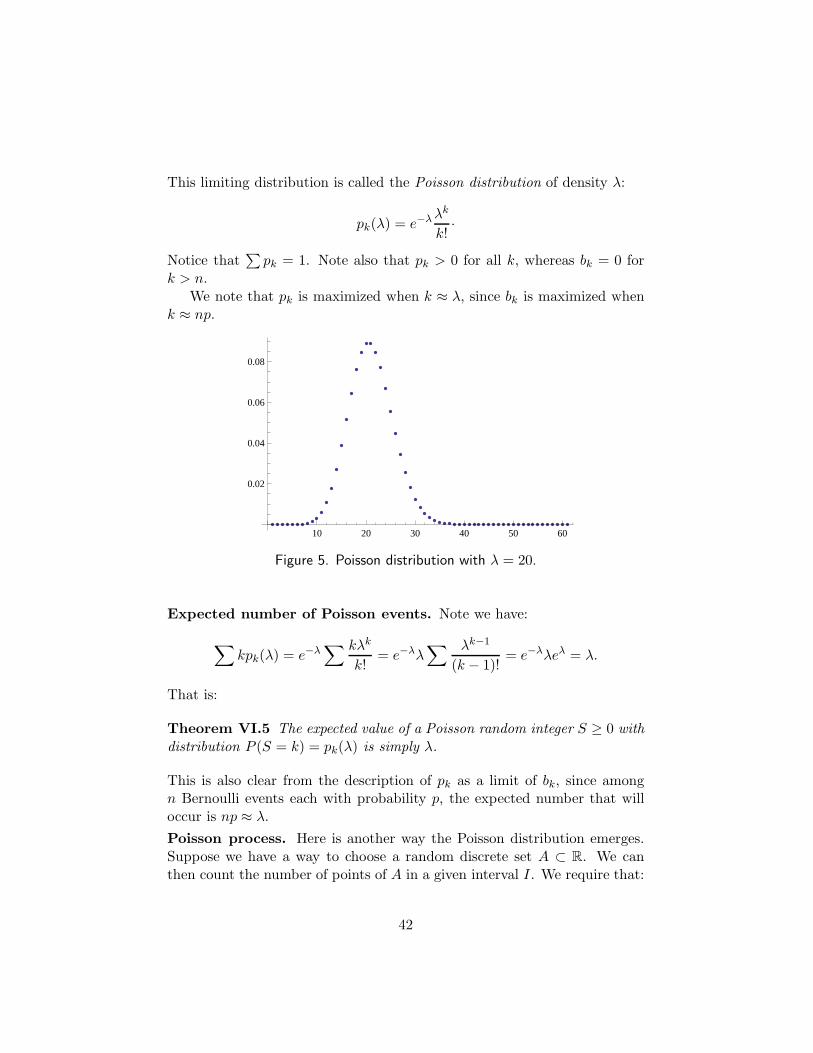
This limiting distribution is called the Poisson distribution of density λ:
pk(λ) = e−λ λk
k!·
Notice that∑
pk = 1. Note also that pk > 0 for all k, whereas bk = 0 fork > n.
We note that pk is maximized when k ≈ λ, since bk is maximized whenk ≈ np.
10 20 30 40 50 60
0.02
0.04
0.06
0.08
Figure 5. Poisson distribution with λ = 20.
Expected number of Poisson events. Note we have:
∑kpk(λ) = e−λ
∑ kλk
k!= e−λλ
∑ λk−1
(k − 1)!= e−λλeλ = λ.
That is:
Theorem VI.5 The expected value of a Poisson random integer S ≥ 0 withdistribution P (S = k) = pk(λ) is simply λ.
This is also clear from the description of pk as a limit of bk, since amongn Bernoulli events each with probability p, the expected number that willoccur is np ≈ λ.
Poisson process. Here is another way the Poisson distribution emerges.Suppose we have a way to choose a random discrete set A ⊂ R. We canthen count the number of points of A in a given interval I. We require that:
42

If I and J are disjoint, then the events |A∩I| = k and |A∩J | = ℓare independent.
The expected value of |A ∩ I| = λ|I|.
Under these assumptions, we have:
Theorem VI.6 The probability that |A ∩ I| = k is given by the Poissondistribution pk(λ|I|).
Proof. Cut up the interval I into many subintervals of length |I|/n. Thenthe probability that one of these intervals is occupied is p = λ|I|/n. Thus theprobability that k are occupied is given by the binomial coefficient bk(n, p).But the number of occupied intervals tends to |A ∩ I| as n → ∞, andbk(n, p) → pk(λ|I|) since np = λ|I| is constant.
The bus paradox. If buses running regularly, once every 10 minutes, thenthe expected number of buses per hour is 6 and the expected waiting timefor the next bus is 5 minutes.
But if buses run randomly and independently — so they are distributedlike a Poisson process — at a rate of 6 per hour, then the expected waitingtime for the next bus is 10 minutes.
This can be intuitively justified. In both cases, the waiting times T1, . . . , Tn
between n consecutive buses satisfy (T1 + · · ·+ Tn)/n ≈ 10 minutes. But inthe second case, the times Ti all have the same expectation, so E(T1) = 10minutes as well. In the first case, only T1 is random; the remaining Ti areexactly 10 minutes.
Here is another useful calculation. Suppose a bus has just left. Inthe Poisson case, the probability that no bus arrives in the next minuteis p0(1/10) = e−1/10 ≈ 1 − 1/10.
Thus about 1 time in 10, another bus arrives just one minute after thelast one. By the same reasoning we have find:
Theorem VI.7 The waiting time T between two Poisson events with den-sity λ is exponentially distributed, with
P (T > t) = p0(λt) = exp(−λt).
Since exp(−3) ≈ 5%, one time out of 20 you should expect to wait morethan half an hour for the bus. And by the way, after waiting 29 minutes,the expected remaining wait is still 10 minutes!
43
Clustering. We will later see that the waiting times Ti are example ofexponentially distributed random variables. For the moment, we remarkthat since sometimes Ti ≫ 10, it must also be common to have Ti ≪ 10.This results in an apparent clustering of bus arrivals (or clicks of a Geigercounter).
Poisson distribution in other spaces. One can also discuss a Poissonprocess in R
2. In this case, for any region U , the probability that |A∩U | = kis pk(λ area(U)). Rocket hits on London during World War II approximatelyobeyed a Poisson distribution; this motif appears in Pynchon’s Gravity’sRainbow.
The multinomial distribution. Suppose we have an experiment with spossible outcomes, each with the same probability p = 1/s. Then after ntrials, we obtain a partition
n = n1 + n2 + · · · + ns,
where ni is the number of times we obtained the outcome i. The probabilityof this partition occurring is:
s−n n!
n1!n2! · · ·ns!·
For example, the probability that 7n people have birthdays equally dis-tributed over the 7 days of the week is:
pn = 7−7n (7n!)
(n!)7·
This is even rarer than getting an equal number of heads and tails in 2ncoin flips. In fact, by Stirling’s formula we have
pn ∼ 7−7n(2π)−3(7n)7n+1/2n−7n−7/2 = 71/2(2π)−3n−3.
For coin flips we had pn ∼ 21/2(2π)−1/2n−1/2 = 1/√
πn. A related calcula-tion will emerge when we study random walks in Z
d.If probabilities p1, . . . , ps are attributed to the different outcomes, then
in the formula above s−n should be replaced by pn1
1 · · · pns
s .
VII Normal Approximation
We now turn to the remarkable universal distribution which arises fromrepeated trials of independent experiments. This is given by the normal
44

density function or bell curve (courbe de cloche):
n(x) =1√2π
exp(−x2/2).
Variance and standard deviation. Let X be a random variable withE(X) = 0. Then the size of the fluctuations of X can be measured by itsvariance,
Var(X) = E(X2).
We also have Var(aX) = a2 Var(X). To recover homogeneity, we define thestandard deviation by
σ(X) =√
Var(X);
then σ(aX) = |a|σ(X).Finally, if m = E(X) 6= 0, we define the variance of X to be that of the
mean zero variable X − m. In other words,
Var(X) = E(X2) − E(X)2 ≥ 0.
The standard deviation is defined as before.
Proposition VII.1 We have Var(X) = 0 iff X is constant.
Thus the variance is one measure of the fluctuations of X.
Independence. The bell curve will emerge from sums of independentrandom variables. We always have E(X +Y ) = E(X)+E(Y ) and E(aX) =aE(X), but it can be hard to predict E(XY ). Nevertheless we have:
Theorem VII.2 If X and Y are independent, then E(XY ) = E(X)E(Y ).
Proof. We are essentially integrating over a product sample space, S ×T . More precise, if s and t run through the possible values for X and Yrespectively, then
E(XY ) =∑
s,t
stP (X = s)P (Y = t)
=(∑
sP (X = s))(∑
tP (Y = t))
= E(X)E(Y ).
45

Corollary VII.3 If X and Y are independent, then Var(X+Y ) = Var(X)+Var(Y ).
Proof. We may assume E(X) = E(Y ) = 0, in which case E(XY ) = 0 andhence E((X + Y )2) = E(X) + E(Y ).
This formula is reminiscent of the Pythagorean formula; indeed, in asuitable vector space, the vectors X and Y are orthogonal.
-4 -2 2 4
0.1
0.2
0.3
0.4
Figure 6. The normal distribution of mean zero and standard deviation one.
Standard deviation of Bernoulli sums. Consider the easy case of therandom variable Sn =
∑n1 Xi, where Xi are independent variables, Xi = 1
with probability p and 0 with probability q = 1 − p. Then X2i = Xi, so
E(Xi) = E(X2i ) = p and hence
Var(Xi) = p − p2 = pq and σ(Xi) =√
pq.
ConsequentlyVar(Sn) = npq and σ(Sn) =
√npq.
The normal random variable. We now turn to the normal distributionand its associated random variable. To begin we establish the importantfact that
∫n(x) dx = 1. This explains the factor of (2π)−1/2. To see this,
we use the following trick:
(∫ ∞
−∞e−x2/2 dx
)2
=
∫ ∫e−(x2+y2)/2 dx dy = 2π
∫ ∞
0e−r2/2r dr = 2π.
46
We remark that there is no simple formula for the antiderivative of n(x), sowe simply define the normal distribution by
N(x) =
∫ x
−∞n(y) dy,
so N ′(x) = n(x). We have just shown N(x) → 1 as x → ∞.We can regard n(x) as giving the distribution of a random variable X.
To obtain the value of X, you choose a point under the graph of n(x) atrandom, and the take its x-coordinate.
Put differently, we have
P (s ≤ X ≤ t) =
∫ t
sn(x) dx = N(t) − N(s).
Note that n(x) → 0 very rapidly as |x| → ∞.
Expectation, variance and standard deviation. By symmetry, wehave E(X) = 0. More precisely,
E(X) =
∫xn(x) dx = 0
because xn(x) is an odd function.What about V = E(X2)? This is called the variance of X. It can be
computed by integrating x2 against the density of the variable X: we have
V =
∫x2
n(x) dx.
To carry out this computation, we integrate by parts. No boundary termsappear because of the rapid decay of n(x); thus we find:
∫x2e−x2/2 dx =
∫xd(−e−x2
/2) =
∫e−x2/2 dx.
Putting back in the (2π)−1/2 gives V = 1.The standard deviation is given by σ(X) = V (X)1/2, so σ(X) = 1 as
well. This justifies the following terminology:
X is a normally distributed random variable of mean zero andstandard deviation one.
47
Exercise: compute∫
x2nn(x) dx.
Properties. The most important property of X is that its values areclustered close to its mean 0. Indeed, we have
P (|X| ≤ 1) = N(1) − N(−1) = 68.2%,
P (|X| ≤ 2) = N(2) − N(−2) = 95.4%,
P (|X| ≤ 3) = N(3) − N(−3) = 99.7%,
P (|X| ≤ 4) = N(4) − N(−4) = 99.994%, and
P (|X| > 4) = 2(1 − N(4)) = 0.0063%.
The event |X| > kσ is sometimes called a k-sigma event. For k ≥ 3 they arevery rare. One can show that
P (X > x) = 1 − N(x) ∼ n(x)/x.
Indeed, integrating by parts we have
1−N(x) =1√2π
∫ ∞
xe−u2/2 du
1√2π
∫ ∞
x
d(−e−u2/2)
u=
n(x)
x+
∫ ∞
x
n(u) du
u2,
and the final integral is negligible compared to the preceding term, whenx ≫ 0.
Flips of a coin and random walks. We will now show that the finalpoint Sn of a random walk of length n behaves like a normally distributedrandom variable of mean 0 and standard deviation
√n. What this means
precisely is:
Theorem VII.4 For any fixed α < β, we have
P (α√
n < Sn < β√
n) → N(β) − N(α)
as n → ∞.
For example, after 10,000 flips of a coin, the probability that the numberof heads exceeds the number of tails by more than 100s is approximatelyby N(−s) (take α = −∞ and β = −s
√n). For example, a difference of 100
should occur less than 16% of the time; a difference of 200, with probabilityless than 2.2%.
This result is not totally unexpected, since we can write Sn =∑n
1 Xi
with Ei independent and E(Xi) = 0, E(X2i ) = 1, and thus E(Sn) = 0 and
E(S2n) = n.
48
Proof. Let us rephrase this result in terms of the binomial distribution forp = q = 1/2. It is convenient to take 2n trials and for −n ≤ k ≤ n, set
ak = bn+k = 2−2n
(2n
n + k
).
This is the same as P (S2n = 2k). We have already seen that
a0 = 2−2n
(2n
n
)∼ 1√
πn·
Also we have a−k = ak.Now let us suppose k is fairly small compared to n, say k ≤ C
√n. We
have
ak = a0 ·n(n − 1) · · · (n − k + 1)
(n + 1)(n + 2) · · · (n + k)= a0 ·
(1 − 0
n
)(1 + 1
n
) ·(1 − 1
n
)(1 + 2
n
) · · ·(1 − k−1
n
)(1 + k
n
) ·
Approximating 1 − x and 1/(1 + x) by e−x, we obtain
ak ≈ a0 exp(−(1 + 3 + 5 + · · · 2k − 1)/n) ≈ a0 exp(−k2/n).
(Note that (1 + 3 + · · · 2k − 1) = k2, as can be seen by layering a picture ofa k × k square into L-shaped strips). Here we have committed an error of(k/n)2 in each of k terms, so the total multiplicative error is 1+O(k3/n2) =1 + O(1/
√n). Thus the ratio between the two sides of this equation goes to
zero as n → ∞.If we set xk = k
√2/n, so ∆xk =
√2/n, then x2
k/2 = k2/n and hencewe have
ak ∼ a0 exp(−x2k/2) ∼
exp(−x2k/2)√
πn∼ n(xk)∆xk.
Recalling that ak = P (S2n = 2k), this gives:
P (α√
2n < S2n < β√
2n) =
β√
n/2∑
k=α√
n/2
ak ∼β∑
xk=α
n(xk)∆xk
→∫ β
αn(x) dx = N(β) − N(α)
as claimed.
49
Corollary VII.5 In a random walk of length n ≫ 0, the quantity Sn/√
nbehaves like a normal random variable of mean zero and standard deviationone.
Stirling’s formula revisited. We did not actually prove that the constantin Stirling’s formula is
√2π. We can now explain how to fill this gap. We
did show that a0 ∼ C/√
n for some constant C. On the other hand, wealso know that
∑n−n ak = 1. Using the fact that
∫n(x) dx = 1, and the
asymptotic expression in terms of a0 above, we find C = 1/√
π and hencethe constant in Stirling’s formula is
√2π.
Normal approximation for general Bernoulli trials. We now turn tothe case of general Bernoulli trials, where 0 < p < 1 and q = 1 − p. In thiscase we let Sn be the number of successes in n trials. As usual we have
P (Sn = k) = bk =
(n
k
)pkqn−k.
We can think of Sn as the sum X1 + · · ·Xn, where Xi are independentvariables and Xi = 1 with probability p and Xi = 0 with probability q.
We now have E(Xi) = p and
Var(Ei) = E((Xi − p)2) = q(−p)2 + pq2 = qp2 + pq2 = pq.
By a similar calculation we have E(Sn) = np and Var(Sn) = npq, and hencethe standard deviation of Sn is given by
σn =√
pqn.
Note that σ is maximized when p = q = 1/2; the spread of the bell curve isless whenever p 6= 1/2, because the outcomes are more predictable.
We can now state the DeMoivre–Laplace limit theorem. Its proof issimilar to the one for p = 1/2, with just more book-keeping. We formulatetwo results. The first says if we express the deviation from the mean interms of standard deviations, then we get an asymptotic formula for thebinomial distribution bk in terms of n(x).
Theorem VII.6 For m = [np] and k = o(n2/3), we have
bm+k ∼ n(xk)∆xk,
where σn =√
npq, xk = k/σn, and ∆xk = 1/σn.
50

Note that we allow k to be a little bigger that√
n, since in the proofwe only needed k3/n2 → 0. This small improvement will lead to the StrongLaw of Large Numbers.
The second shows how the normal distribution can be used to measurethe probability of deviations from the mean.
Theorem VII.7 As n → ∞ we have
P (ασn < Sn − np < βσn) → N(β) − N(α).
Put differently, if we set Xn = (Sn − np)/√
npq, this gives
P (α < Xn < β) → N(β) − N(α).
That means Xn behaves very much like a the standard normal randomvariable X of mean zero and standard deviation one. Thus when suitablynormalized, all outcomes of repeated random trials are (for large n) governedby a single law, which depends on p and q only through the normalization.
How does√
pq behave? It is a nice exercise to graph σ(p) =√
pq as afunction of p ∈ [0, 1]. One finds that σ(p) follows a semicircle of radius 1/2centered at p = 1/2. In other words, σ2 + (p − 1/2)2 = 1/4.
Examples: coins and dice. Let us return to our basic examples. Consideragain n = 10,000 flips of a coin. Then p = q = 1/2 so σ =
√n/2 = 50.
So there is a 68% chance that the number of heads Sn lies between 4,950and 5,050; and less than a 2% chance that Sn exceeds 5,100; and Sn shouldexceed 5,200 only once is every 31,050 trials (i.e. even a 2% error is extremelyunlikely). (Note that these answers are shifted from those for random walks,which have to do with the difference between the number of heads and tails.)
Now let us analyze 10, 000 rolls of a die. In this case σ =√
n(1/6)(5/6) =√5n/6 ≈ 0.373
√n ≈ 37 is somewhat less than in the case of a fair coin (but
not 3 times less!). We expect an ace to come up about 1,666 times, and 68%of the time the error in this prediction is less than 37.
Median deviation. What is the median deviation from the mean? It turnsout that N(α)−N(−α) = 0.5 for α ≈ 0.6745 ≈ 2/3. (This is also the valuesuch that N(α) = 3/4, since N(−α) = 1 − N(α).) Thus we have:
Theorem VII.8 The median deviation of a normal random variable is ≈0.6745σ. That is, the events |X| < 0.6745σ and |X| > 0.6745σ are equallylikely, when E(X) = 0.
51
For 10,000 flips of a fair coin, we have a median deviation of about 33flips; for dice, about 24 rolls.
By convention a normalized IQ test has a mean of 100 and a standarddeviation of 15 points. Thus about 50% of the population should have anIQ between 90 and 110. (However it is not at clear if actual IQ scores fit thenormal distribution, especially for high values which occur more frequentlythan predicted.)
Voter polls, medical experiments, conclusions based on small sam-ples, etc. Suppose we have a large population of N voters, and a fractionp of the population is for higher taxes. We attempt to find p by polling nmembers of the population; in this sample, np′ are for higher taxes. Howconfident can we be that p′ is a good approximation to p?
Assuming N ≫ n, the polling can be modeled on n independent Bernoullitrials with probability p, and an outcome of Sn = np′. Unfortunately wedon’t know p, so how can we find the standard deviation? We observe thatthe largest σ can be occurs when p = q = 1/2, so in any case we haveσn ≤ √
n/2. Consequently we have
P (|p′ − p| ≤ α) = P (|Sn − np| ≤ nα) ≥ P (|Sn − np| ≤ 2α√
nσn)
≈ N(2α√
n) − N(−2α√
n).
So for example, there is at most a 95% chance (2σ chance) that |p−p′| is lessthan α = 1/
√n. So if we want an error α of at most 0.5%, we can achieve
this with a sample of size n = α−2 = 40, 000 about 95% of the time.Most political polls are conducted with a smaller number of voters, say
n = 1000. In that case σ ≤ 1/√
1000 ≈ 16. So there is a 68% chance thepoll is accurate to with 16/1000 = 1.6% Errors of four times this size arevery unlikely to occur (they are 4σ events). However:
The practical difficulty is usually to obtain a representative sam-ple of any size.
—Feller, vol. I, p.190.
When nothing is found. If one knows or is willing to posit that p is rathersmall — say p ≤ 1/25 — then a somewhat smaller sample is required, sincewe can replace
√pq ≤ 1/2 by
√pq ≤ 1/5. (Of course an error of a few
percent may be less tolerable when the answer p is already down to a fewpercent itself.)
An extreme case is when a poll of n voters turns up none who are infavor of a tax increase. In this case simpler methods show that p ≤ C/n with
52
good confidence. Indeed, if p > C/n then the probability of total failure isabout (1 − p)n ≈ exp(−C). We have e−3 ≈ 0.05 so we have 95% confidencethat p ≤ 3/n.
This provides another approach to Laplace’s estimate for the probabilitythe sun will rise tomorrow.
Normal approximation to the Poisson distribution. We recall thatthe Poisson distribution pk(λ) describe the limiting distribution of bk asn → ∞ and np → λ. Thus it describes a random variable S — the numberof successes — with E(S) = λ. The variance of the binomial distribution isnpq → λ as well, so we expect Var(S) = λ and σ(S) =
√λ.
We can also see this directly. Let
f(µ) = exp(−λ)
∞∑
0
µk
k!= exp(µ − λ).
Then f(λ) =∑
pk(λ) = 1. Next note that
µf ′(µ) = exp(−λ)
∞∑
0
kµk
k!= µ exp(µ − λ).
Thus λf ′(λ) =∑
kpk(λ) = E(S) = λ. Similarly,
(µ
d
dµ
)2
f = exp(−λ)
∞∑
0
k2µk
k!= (µ2 + µ) exp(µ − λ),
and hence E(S2) = λ2 + λ, whence
Var(S) = E(S2) − E(S2) = λ.
With these observations in place, the following is not surprising; compareFigure 5.
Theorem VII.9 As λ → ∞, we have
P (α < (S − λ)/√
λ < β) → N(β) − N(α).
Similarly, we have
Theorem VII.10 For m = [λ] and k = O(λ2/3), we have
pm+k ∼ n(xk)∆xk,
where xk = k/√
λ and ∆xk = 1/√
λ.
53
Example: call centers. The remarkable feature of the Poisson distribu-tion is that the standard deviation is determined by the mean. Here is anapplication of this principle.
The Maytag repair center handles on average 2500 calls per day. Byoverstaffing, it can handle an additional n calls per day. How large shouldn be to insure that every single call is handled 99 days out of 100?
We model the daily call volume V by the Poisson distribution (assuminga large base of mostly trouble-free customers), with expected value λ = 2500.Then the standard deviation is σ =
√λ = 50. From the above, we have
P (V < 2500 + 50s) ≈ N(s),
and N(s) = 0.99 when s = 2.33. Thus by adding staff to handle n =2.33 · 50 = 117 extra calls, we can satisfy all customers 99 days out of 100.Without the extra staffing, the support center is overloaded half the time.A 5% staff increase cuts the number of days with customer complaints by afactor of 50.
Large deviations. Using Theorem VII.6, we can now get a good bound onthe probability that Sn is nǫ standard deviations from its mean. This boundis different from, and more elementary than, the sharper bounds found inFeller; but it will be sufficient for the Strong Law of Large Numbers. (Tohave an idea of the strength of this bound, note that exp(−nδ) tends to zerofaster than 1/nk for any k > 0, as can be checked using L’Hopital’s rule.)
Theorem VII.11 For any ǫ > 0 there is a δ > 0 such that
P (|Sn − np| > n1/2+ǫ) = O(exp(−nδ)).
Proof. The probability to be estimated is bounded by nbnp+k, where k =n1/2+ǫ (with implicit rounding to whole numbers). We may assume 0 < ǫ <1/6, so Theorem VII.6 applies, i.e. we have k = o(n2/3). Recall σn =
√npq,
so x = k/σn > Cnǫ > 0 for some constant C (depending on p, q), and∆x = 1/σn = O(1/
√n). Thus
nbnp+k ∼ nn(x)∆x = O(√
n exp(−x2/2)).
Since x ≫ nǫ, we have x2/2 ≫ n2ǫ. Thus we can choose δ > 0 suchthat nδ < x2/4 for all n sufficiently large. We can also drop the factorof
√n, since exp(−nδ) tends to zero faster than any power of n. Thus
nbnp+k = O(exp(−nδ)) as desired.
With a more careful argument, one can actually show that the probabil-ity above is asymptotic to 1 − N(xn), where xn = nǫ/
√pq.
54

VIII Unlimited Sequences of Bernoulli Trials
In this section we study infinite sequence of coin flips, dice throws and moregeneral independent and sometimes dependent events.
Patterns. Let us start with a sequence of Bernoulli trials Xi. with 0 < p <1. A typical outcome is a binary sequence (Xi) = (0, 1, 1, 0, 0, 0, 1, . . .). Wesay a finite binary pattern (ǫ1, . . . , ǫk) occurs if there is some i such that
(Xi+1, . . . ,Xi+k) = (ǫ1, . . . , ǫk).
Theorem VIII.1 With probability one, every pattern occurs (infinitely of-ten).
In finite terms this means pn → 1, where pn is probability that the givenpattern occurs during the first n trials. One also says the pattern occursalmost surely.
Proof. Let Ai be the event that the given pattern occurs starting in positioni + 1. Then A0, Ak, A2k etc. are independent events, and each has thesame probability s of occurring. Since 0 < p < 1, we have s > 0. So theprobability that the given pattern does not occur by epoch nk is less thanP (A′
0 · · ·A′n) = (1 − s)n → 0.
As a special case: so long as p > 0, there will be infinitely many successesa.s. (almost surely).
Infinite games. For example, suppose we flip a fair coin until either 3heads come up in a row or two tails in a row. In the first case we win, and inthe second case we lose. The chances of a draw are zero, since the patternsHHH and TT occur infinitely often (almost surely); it is just a question ofwhich occurs first.
To calculate the probability P (A) of a win, let H1 be the event that thefirst flip is heads, and T1 the event that it is tails. Then
P (A) = (P (A|H1) + P (A|T1))/2.
Next we claim:P (A|H1) = 1/4 + (3/4)P (A|T1).
This is because either we see two more heads in a row and win (with prob-ability 1/4), or a tail comes up, and then a winning sequence for a playbeginning with a tail. Similarly we have:
P (A|T1) = P (A|H1)/2,
55
since either we immediately flip a head, or we lose. Solving these simul-taneous equations, we find P (A|H1) = 2/5, P (A|T1) = 1/5, and henceP (A) = 3/10.
The Kindle Shuffle. It would not be difficult to produce a hand-heldreading device that contains not just ever book every published, but everybook that can possibly be written. As an add bonus, each time opened itcould shuffle through all these possibilities and pick a new book which youprobably haven’t read before. (Engineering secret: it contains a small chipthat selects letters at random until the page is full. It requires much lessoverhead than Borges’ Library of Babel.)
Backgammon. The game of backgammon includes an unlimited sequenceof Bernoulli trials, namely the repeated rolls of the dice. In principle, thegame could go on forever, but in fact we have:
Theorem VIII.2 (M) Backgammon terminates with probability one.
Proof. It is easy to see that both players cannot be stuck on the bar forever.Once at least one player is completely off the, a very long (but universallybounded) run of rolls of 2 − 4 will force the game to end. Such a run musteventually occur, by the second Borel–Cantelli lemma.
The doubling cube also provides an interesting, simpler exercise.
Theorem VIII.3 Player A should double if his chance of winning is p >1/2. Player B should accept if p ≤ 3/4.
Proof. The expected number of points for player A changes from p − q to2(p − q) upon doubling, and this is an improvement provided p > 1/2. Theexpected point for player B change from −1 to 2(q−p) upon accepting, andthis is an improvement if 2(p − q) < 1 — that is, if p < 3/4.
When p > 3/4 one says that player A has lost his market.
The Borel-Cantelli lemmas. We now consider a general infinite sequenceof events A1, A2, . . .. A finite sample space has only finitely many events;these results are useful only when dealing with an infinite sample space, suchas an infinite random walk or an infinite sequence of Bernoulli trials. Notethat the expected number of events which occur is
∑P (Ai).
Theorem VIII.4 If∑
P (Ai) < ∞, then almost surely only finitely manyof these events occur.
56
Proof. The probability that N or more events occur is less than∑∞
N P (Ai)and this tends to zero as N → ∞.
One might hope that∑
P (Ai) = ∞ implies infinitely many of the Ai
occur, but this is false; for example, if A1 = A2 = · · · then the probabilitythat infinitely many occur is the same as P (A1). However we do get a resultin this direction if we have independence.
Theorem VIII.5 If the events Ai are independent, and∑
P (Ai) = ∞,then almost surely infinitely many of them occur.
Proof. It suffices to show that almost surely at least one of the eventsoccurs, since the hypothesis holds true for {Ai : i > n} .But the probabilitythat none of the events occurs is bounded above by
pn = P (A′1 · · ·A′
n) =n∏
1
(1 − P (Ai)),
and this tends to zero as n → ∞ since∑
P (Ai) diverges.
Example: card matching. Consider an infinite sequence of games in-dexed by n. To play game n, you and your opponent each choose a numberfrom 1 to n. When the numbers match, you win a dollar. Let An be theevent that you win the nth game. If you choose your number at random, in-dependently each time, then P (An) = 1/n, and by the second Borel-Cantellilemma you will almost surely win as much money as you could ever want.(Although it will take about en games to win n dollars.)
Now let us modify the game so it involves 2n numbers. Then if youropponent chooses his number at random, we have P (An) = 2−n. There isno bound to the amount you can win in this modified game, but now it isalmost certain that the limit of winnings as n → ∞ will be finite.
Finally let us consider the St. Petersburg game, where chances of winningremaining 2−n but the payoff is 2n. Then your expected winnings are infinite,even though the number of times you will win is almost surely finite.
Example: Fermat primes and Mersenne primes. Fermat conjecturedthat every number of the form Fn = 22n
+ 1 is prime. Mersenne and othersconsidered instead the sequence Mn = 2n −1; these can only be prime whenn is prime.
It is a good heuristic that the ‘probability’ a number of size n is primeis 1/ log n. (In fact, the prime number theorem states the number of primes
57
p ≤ n is asymptotic to n/ log n.) Thus the probability that Mn is primeis about 1/n, and since
∑1/n diverges, it is conjectured that there are
infinitely many Mersenne primes. (Equivalently, there are infinitely manyeven perfect numbers, since these all have the form 2p−1(2p − 1) with thesecond factor prime.)
On the other hand, we have 1/ log Fn ≍ 2−n, so it is conjectured thatthere are only finitely many Fermat primes.
There are in fact only 5 known Fermat primes: 3, 5, 17, 257, and 65537.At present there are about 47 known Mersenne primes, the largest of whichis on the order of 1024.
The law of large numbers. We can now formulate a stronger law of largenumbers for Bernoulli trials. Before we showed that P (|Sn/n− p| > ǫ) → 0.But this could still allow fluctuations of size ǫ to occur infinitely often.
The stronger law is this:
Theorem VIII.6 With probability one, Sn/n → p.
Proof. Fix α > 0, and consider the events
An = (|Sn/n − p| > α) = (|Sn − np| > αn).
By Borel–Cantelli, what we need to show is that∑
P (An) < ∞ no matterwhat α is. Then An only happens finitely many times, and hence Sn/n → p.
Recall that σn = σ(Sn) =√
npq. Let us instead fix 0 < ǫ and considerthe event
Bn = (|Sn − np| > n1/2+ǫ).
Clearly An ⊂ Bn for all n ≫ 0, so it suffices to show∑
P (Bn) < ∞. Butby Theorem VII.11, there is a δ > 0 such that
P (Bn) = O(exp(−nδ)).
Now notice that nδ > 2 log n for all n ≫ 0, and hence P (Bn) = O(1/n2).Since
∑1/n2 converges, so does
∑exp(−nδ), and the proof is complete.
The law of the iterated logarithm. We conclude with an elegant resultdue to Khintchine, which says exactly how large the deviations should getin a infinite sequence of Bernoulli trials.
Let S∗n = (Sn −np)/
√npq be the number of standard deviations that Sn
deviates from its expect value np.
58
Theorem VIII.7 We have
lim supS∗
n√2 log log n
= 1
almost surely.
This means S∗n will get bigger than
√(2 − ǫ) log log n infinitely often. In
particular we will eventually see an event with 10 standard deviations, butwe may have to wait a long time (e.g. until 2 log log n = 100, or equivalentlyn = exp(exp(50)) ≈ 101021
).Here is a weaker form that is easier to prove:
Theorem VIII.8 We have lim supS∗n = ∞.
Proof. Choose nr → ∞ such that√
nr+1 ≫ nr; for example, one cantake nr = 22r
. Let T ∗r be the deviation of the trials (nr + 1, . . . , nr+1 − 1)
measured in standard deviations. Now at worst, the first nr trials were allfailures; but nr is much smaller than the standard deviation
√nr+1, so we
still have T ∗r = S∗
nr+ o(1). Now the events
Ar = (T ∗r > x)
are independent, and by the normal approximation they satisfy
P (Ar) ∼ 1 − N(x) > 0,
so∑
P (Ar) = +∞ and hence
lim sup S∗n ≥ lim supT ∗
r ≥ x > 0.
Since x was arbitrary, we are done.
Sketch of the proof of Theorem VIII.7. The proof is technical butstraightforward. Using the Borel-Cantelli lemma, it all turns on whether ornot a certain sum converges. To give the idea we will show
lim supS∗
n√2 log log n
≤ 1.
The first point is that any small lead in Sn−np has about a 50% probabilityof persisting till a later time, since about half the time Sn is above itsexpected value. So roughly speaking,
P (Sk − kp > x for some k < n) ≤ P (Sn − np > x)/2.
59
Now pick any numbers 1 < γ < λ. We will show the limsup above is lessthan λ. Let nr = γr, and let
Ar = (Sn − np ≥ λ√
2npq log log n for some n, nr ≤ n ≤ nr+1).
Then we have
2P (Ar) ≤ P (Snr+1− nr+1p ≥ λ
√2nrpq log log nr).
The standard deviation of Snr+1is√
nr+1pq =√
γnrpq, so in terms of stan-dard deviations the event above represents a deviation of
xr = λ√
2γ−1 log log nr ≥√
λ log log nr
(since λ > γ). By the normal approximation, we then have
P (Ar) ≤ exp(−x2r/2) = exp(−λ log log nr) = (log nr)
−λ =1
(r log γ)λ·
Since∑
r 1/rλ < ∞ for any λ > 1, the first Borel-Cantelli lemma shows onlyfinitely many of these events happen. Hence the limsup is at most one.
IX Random Variables and Expectation
A random variable is a function X : S → R. In this section we give asystematic discussion of random variables.
Distribution. Let us assume S is discrete with probability function p(s).Then X assumes only countably many values, say x1, x2, . . . ,. The numbersP (X = xi) give the distribution of X.
We have often met the case where X : S → Z. In this case the distribu-tion of X is recorded by the numbers
pk = P (X = k) =∑
s:X(s)=k
p(s).
We always have∑
pk = 1.
Expected value. The average, mean or expected value is given by
E(X) =∑
S
p(s)X(s) =∑
xiP (X = xi).
60

In the case of an integer-valued random variable, it is given by
E(X) =∑
kpk.
(These sums might not converge absolutely, in which case we say the ex-pected value does not exist.) Clearly E is linear:
E(∑
aiXi
)=∑
aiE(Xi).
Examples.
1. For a single Bernoulli trial we have p0 = q and p1 = p, and E(X) = p.
2. For Sn, the number of successes in n Bernoulli trials, we have
pk =
(n
k
)pkqn−k.
We have E(Sn) = np.
3. If X obeys a Poisson distribution then
pk = e−λ λk
k!,
and E(X) = λ.
4. The moment X = k at which a random walk first returns to the originis distributed according to:
p2n =1
22n(2n − 1)
(2n
n
)·
We have pk = 0 if k is odd. We have also seen then 2np2n ∼√
1√
πn,so E(X) = +∞.
5. The time X = k of the first success in a sequence of Bernoulli trialsobeys the geometric distribution:
pk = pqk−1.
This is because all the preceding events must be failures. We haveE(X) = 1/p.
61
Generating functions. (See Feller, Ch. XI for more details.) When Xonly takes integer values k ≥ 0, and these with probability pk, the distribu-tion of X is usefully recorded by the generating function
f(t) =∞∑
0
pktk.
Note that f(1) = 1, and f ′(1) = E(X).
Examples.
1. For the binomial distribution for n trials with probability p, we have
f(t) =∑(
n
k
)pkqn−ktk = (q + tp)n.
2. For the Poisson distribution with expected value λ, we have
f(t) = e−λ∑ λktk
k!= exp(λt)/ exp(λ).
3. For the geometric distribution pk = qk−1p, we have
f(t) = p
∞∑
1
qk−1tk =pt
1 − tq·
Theorem IX.1 The generating function for a sum of independent randomvariables X1 + X2 is given by f(t) = f1(t)f2(t).
Proof. The distribution of the sum is given by
pk =∑
i+j=k
P (X1 = i and X2 = j) =∑
i+j=k
p1i p
2j .
Corollary IX.2 If Sn =∑n
1 Xi is a sum of independent random variableswith the same distribution, then its generating function satisfies fn(t) =f1(t)
n.
The binomial distribution is a prime example.
62

Corollary IX.3 The sum of two or more independent Poisson randomvariables also obeys the Poisson distribution.
The concept of a random variable. A basic principle is that all proper-ties of X alone are recorded by its distribution function, say pk. That is, thesample space is irrelevant. Alternatively we could suppose S = Z, X(k) = kand p(k) = pk. One can even imagine a roulette wheel of circumference 1meter, with intervals of length pk marked off and labeled k. Then the wheelis spun and the outcome is read off to get X.
For example, we have
E(sin(X)) =∑
sin(pk)pk,
and similarly for any other function of X. In particular E(X) and σ(X) aredetermined by the probability distribution pk.
In the early days of probability theory the sample space was not explicitlymentioned, leading to logical difficulties.
Completing a collection. Each package of Pokemon cards contains 1 ofN possible legendary Pokemon. How many packs do we need to buy to getall N? (Gotta catch ’em all R©.) We assume all N are equally likely witheach purchase.
Let Sr be the number of packs needed to first acquire r legendaries.So S0 = 0 and S1 = 1, but Sr is a random variable for r > 1. WriteXr = Sr+1 − Sr; then Xr is the waiting time for the first success in asequence of Bernoulli trials with probability p = (N − r)/N . We have seenalready that E(Xr) = 1/p = N/(N − r). Thus
E(Sr) = E(X0 + X1 + · · · + Xr−1) = N
(1
N+
1
N − 1+ · · · + 1
N − r + 1
).
(Correction: before (3.3) on p. 225 of Feller, Xr should be Xr−1.) To get acomplete collection the expected number of trials is
E(SN ) = N(1 + 1/2 + 1/3 + · · · 1/N) ∼ N log N.
For N = 10 we get E(SN ) = 29.29, even though E(S5) = 10(1/6 + 1/7 +· · · 1/10) ≈ 6.46.
Note especially that we calculated E(Sr) without every calculating theprobability distribution P (Sr = k). Expectations are often easier to com-pute than distributions.
63

Joint distribution. We can similarly consider two (or more random vari-ables) X and Y . Their behavior is then governed by their joint distribution
pst = P (X = s, Y = t).
For example, if we drop 3 balls into 3 cells, and let X be the number thatland in cell one and N the number of occupied cells. Then we have 27possible configurations, each equally likely. The row and column sums givethe distributions of N and X individually.
N\X 0 1 2 3
1 2/27 0 0 1/27 1/9
2 6/27 6/27 6/27 0 6/9
3 0 6/27 0 0 2/9
8/27 12/27 6/27 1/27 1
Independence. We say X and Y are independent if P (X = s, Y = t) =P (X = s)P (Y = t) for all s and t. A similarly definition applies to morethan two variables.
Clearly X and N above are not independent. As a second example, ina Bernoulli process let X1 be the number of failures before the first success,and let X2 be the number of failures between the first two successes. Then
P (X1 = j,X2 = k) = qj+kp2 = p(X1 = j)P (X2 = k).
These two events are independent.
Random numbers of repeated trials. Let N be a Poisson randomvariable with E(N) = λ, and let S and F denote the number of successesand failures in N Bernoulli trials with probability p. Then
P (S = a, F = b) = P (N = a + b)
(a + b
a
)paqb = e−λ λa+b
(a + b)!
(a + b)!
a!b!paqb
=
(e−pλ (pλ)a
a!
)(e−qλ (qλ)b
b!
).
In other words, S and F are independent Poisson variables with expectationsλp and λq respectively.
To explain this, imagine making a huge batch of muffins with an averageof λ raisins per muffin. Then the number of raisins in a given muffin is
64

distributed by N . Suppose on average pλ raisins are black and qλ are gold.Then S and F give the number of black and gold raisins. Clearly theirdistributions are independent and Poisson.
Covariance. We have previously seen:
Theorem IX.4 If X and Y are independent then E(XY ) = E(X)E(Y )and Var(X + Y ) = Var(X) + Var(Y ).
We can use the failure of these results to hold as one measure of thedependence between X and Y . Namely we define the covariance by
Cov(X,Y ) = E(XY ) − E(X)E(Y ).
Note that like the variance, Cov(X+a, Y +b) = Cov(X,Y ); we can always re-duce to the case of variables with mean zero. It also satisfies Cov(aX, bY ) =abCov(X,Y ) and Cov(X,Y ) = Cov(Y,X). Bilinearity is also very useful:
Cov(X1 + X2, Y ) = Cov(X1, Y ) + Cov(X2, Y ).
Finally note thatVar(X) = Cov(X,X).
Theorem IX.5 We have Var(X + Y ) = Var(X) + Var(Y ) + 2Cov(X,Y ).More generally,
Var(∑
Xi
)=∑
Var(Xi) + 2∑
i<j
Cov(Xi,Xj).
Proof. We can assume mean zero; then in the first case we have
Var(X + Y ) = E((X + Y )2) = E(X2) + E(Y 2) + 2E(XY )
and the result is immediate. The general case is similar.
Here is a variant of the familiar Cauchy–Schwarz inequality, |〈x, y〉|2 ≤‖x‖2 · ‖y‖2.
Theorem IX.6 We have |Cov(X,Y )|2 ≤ Var(X)Var(Y ).
Proof. We may assume both sides have mean zero, and rescale so Var(X) =Var(Y ) = 1. Then 0 ≤ Var(X−Y ) = 2(Var(X)2−Cov(X,Y )) so Cov(X,Y ) ≤Var(X)2 = Var(X)Var(Y ). The reverse inequality comes from the fact thatVar(X + Y ) ≥ 0.
65
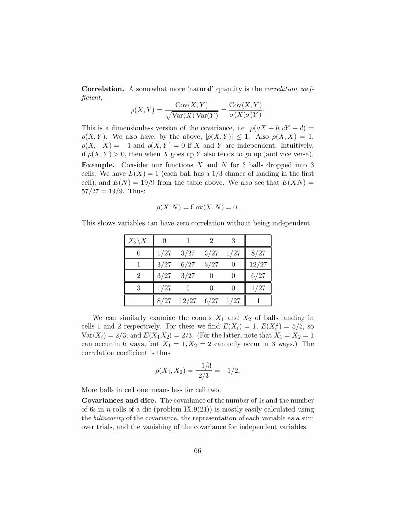
Correlation. A somewhat more ‘natural’ quantity is the correlation coef-ficient,
ρ(X,Y ) =Cov(X,Y )√
Var(X)Var(Y )=
Cov(X,Y )
σ(X)σ(Y )·
This is a dimensionless version of the covariance, i.e. ρ(aX + b, cY + d) =ρ(X,Y ). We also have, by the above, |ρ(X,Y )| ≤ 1. Also ρ(X,X) = 1,ρ(X,−X) = −1 and ρ(X,Y ) = 0 if X and Y are independent. Intuitively,if ρ(X,Y ) > 0, then when X goes up Y also tends to go up (and vice versa).
Example. Consider our functions X and N for 3 balls dropped into 3cells. We have E(X) = 1 (each ball has a 1/3 chance of landing in the firstcell), and E(N) = 19/9 from the table above. We also see that E(XN) =57/27 = 19/9. Thus:
ρ(X,N) = Cov(X,N) = 0.
This shows variables can have zero correlation without being independent.
X2\X1 0 1 2 3
0 1/27 3/27 3/27 1/27 8/27
1 3/27 6/27 3/27 0 12/27
2 3/27 3/27 0 0 6/27
3 1/27 0 0 0 1/27
8/27 12/27 6/27 1/27 1
We can similarly examine the counts X1 and X2 of balls landing incells 1 and 2 respectively. For these we find E(Xi) = 1, E(X2
i ) = 5/3, soVar(Xi) = 2/3; and E(X1X2) = 2/3. (For the latter, note that X1 = X2 = 1can occur in 6 ways, but X1 = 1,X2 = 2 can only occur in 3 ways.) Thecorrelation coefficient is thus
ρ(X1,X2) =−1/3
2/3= −1/2.
More balls in cell one means less for cell two.
Covariances and dice. The covariance of the number of 1s and the numberof 6s in n rolls of a die (problem IX.9(21)) is mostly easily calculated usingthe bilinearity of the covariance, the representation of each variable as a sumover trials, and the vanishing of the covariance for independent variables.
66

Let Ai = 1 when the ith roll is an ace, and zero otherwise. Define Si
similarly for a roll of six. Then
Cov(Ai, Si) = E(AiSi) − E(Ai)E(Si) = −1/36,
and Cov(Ai, Sj) = 0 for i 6= j by independence. Thus
Cov(∑
Ai,∑
Si
)= n Cov(S1, A1) = −n/36.
We also have Var(Ai) = Var(Si) = npq = 5n/36, so we get a correlationcoefficient
ρ(∑
Si,∑
Ai
)= −1/5,
independent of n. By the same reasoning we get:
Proposition IX.7 If (Xi, Yi) have the same joint distribution as (X1, Y1)and these variables are independent for different values of i, then
ρ
(n∑
1
Xi,
n∑
1
Yi
)= ρ(X1, Y1).
We remark that if A and B are Bernoulli trials with the same probabilityp, thought of also as 0/1 functions, then
ρ(A,B) =P (AB) − p2
pq=
P (A|B) − P (A)
q·
For example, if A and B are mutually exclusive, then ρ(A,B) = −p/q.In the dice case this gives −1/5 as above. Note that if P (AB) = 0 thenP (A) + P (B) = 2p ≤ 1 and so p ≤ q. We also note that for mean zerorandom variables, we have
ρ(X,Y ) =E(XY )√
E(X2)E(Y 2)·
Chebyshev’s inequality. There is a very simple and yet useful way tobound the fluctuations in a random variable X of finite variance.
Theorem IX.8 For any random variable X with m = E(X) finite, we have
P (|X − m| > s) ≤ Var(X)/s2.
Proof. We may assume E(X) = 0, and then it is clear that
s2P (|X| > 2) ≤ E(X2) = Var(X).
67
This bound is sometimes quite weak, since in the case of a normal randomvariable with variance 1 we have P (|X| > s) = O(exp(−s2/2)/s). On theother hand if X has a discrete distribution with pk ≍ 1/k3+ǫ, then X hasfinite variance and
P (|X − m| > k) ≍ 1
k2+ǫ·
So in this case Chebyshev’s bound is nearly sharp.
X Law of Large Numbers
In this section we give two applications of Chebyshev’s inequality. First,we generalize the strong law of large numbers beyond Bernoulli trials. Thenew proof is in fact easier that the one given previously, since it does notrely on the normal approximation. Second, we give an application to thecombinatorics of permutations.
Theorem X.1 The strong law of large numbers holds for any set of inde-pendent, uniformly bounded random variables Xk. That is, if Sn = X1 +· · · + Xn and E(Sn/n) = µn, then
|Sn/n − µn| → 0
almost surely as n → ∞.
Proof. We may assume E(Xi) = 0. By boundedness and independence, wehave Var(Sn) = O(n). By Chebyshev’s inequality, P (|Sn| > ǫn) is O(1/n).So if we choose a subsequence ni along which
∑1/ni < ∞, by easy Borel-
Cantelli we have |Sni| < ǫni for all i sufficiently large. By boundedness,
|Sj −Sni| = O(ni+1−ni) = O(di) if ni < j ≤ ni+1. So if we can also arrange
that di = o(ni) we are done, for then
|Sj |j
= O
(di + |Sni
|ni
)
and both di/ni and Sni/ni tend to zero. Note that for ni = λi we do not
have di/ni → 0. But many other choices of ni work, e.g. if ni = i2 then∑1/ni < ∞ and di = O(i) = o(ni) and we are done.
68
This proof illustrates a key technique: we use the fact that Sn is slowlyvarying to transport a conclusion along a sparse subsequence of n to thewhole sequence.
Here is a variant which relaxes the assumption of uniform boundedness.
Theorem X.2 If Xi are independent, identically distributed random vari-ables and µ = E(Xi) is finite, then Sn/n → µ almost surely.
In the result above, the variance of Xi is allowed to be infinite. If it isfinite, however, we have:
Theorem X.3 (Central limit theorem) If, in addition, σ = σ(Xi) isfinite, then
P
(Sn − nµ
σ√
n< x
)→ N(x).
Example: permutations. Here is a combinatorial application whose con-clusions make no reference to probability.
A random permutation π : n → n can be constructed by first choosingπ(1), then choosing π(π(1)), etc. When πk(1) = 1 we have completed acycle; then we start over and choose π(x), where x is the smallest integerfor which π is still undefined.
Let Xk = 1 if a cycle is completed at the kth step (starting with k = 0),and 0 otherwise. Clearly P (X0) = 1/n and in general π(Xk) = 1/(n − k).Thus the average number of cycles of a random permutation is given by
E(∑
Xi
)= E(Sn) = 1 +
1
2+ · · · + 1
n∼ log n.
We also have
Var(X2k) = E(Xk) − E(Xk)
2 ≈ 1
n − k
unless k is close to n. It is a beautiful fact that the variables Xk are indepen-dent; using this, we find that Var(Sn) ∼ log n as well. Then by Chebyshev,most permutations have within O(
√log n) of log n cycles. (In fact the central
limit theorem holds as well.)A related fact: a random sparse graph on n vertices has diameter about
log n.
Application: the median. Let X1,X2, . . . be an arbitrary sequence ofindependent, identically distributed random variables, with density f(x).Their median is the unique value M such that
∫ M
−∞f(x) dx = 1/2.
69
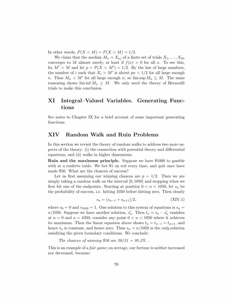
In other words, P (X < M) = P (X > M) = 1/2.We claim that the median Mn = Xn) of a finite set of trials X1, . . . ,X2n
converges to M almost surely, at least if f(x) > 0 for all x. To see this,fix M ′ > M and let p = P (X > M ′) < 1/2. By the law of large numbers,the number of i such that Xi > M ′ is about pn < 1/2 for all large enoughn. Thus Mn < M ′ for all large enough n, so lim supMn ≤ M . The samereasoning shows lim inf Mn ≥ M . We only need the theory of Bernoullitrials to make this conclusion.
XI Integral–Valued Variables. Generating Func-
tions
See notes to Chapter IX for a brief account of some important generatingfunctions.
XIV Random Walk and Ruin Problems
In this section we revisit the theory of random walks to address two more as-pects of the theory: (i) the connection with potential theory and differentialequations, and (ii) walks in higher dimensions.
Ruin and the maximum principle. Suppose we have $1000 to gamblewith at a roulette table. We bet $1 on red every time, and quit once havemade $50. What are the chances of success?
Let us first assuming our winning chances are p = 1/2. Then we aresimply taking a random walk on the interval [0, 1050] and stopping when wefirst hit one of the endpoints. Starting at position 0 < n < 1050, let sn bethe probability of success, i.e. hitting 1050 before hitting zero. Then clearly
sn = (sn−1 + sn+1)/2, (XIV.1)
where s0 = 0 and s1050 = 1. One solution to this system of equations is sn =n/1050. Suppose we have another solution, s′n. Then tn = sn − s′n vanishesat n = 0 and n = 1050; consider any point 0 < n < 1050 where it achievesits maximum. Then the linear equation above shows tn = tn−1 = tn+1, andhence tn is constant, and hence zero. Thus sn = n/1050 is the only solutionsatisfying the given boundary conditions. We conclude:
The chances of winning $50 are 20/21 = 95.2% .
This is an example of a fair game; on average, our fortune is neither increasednor decreased, because:
70
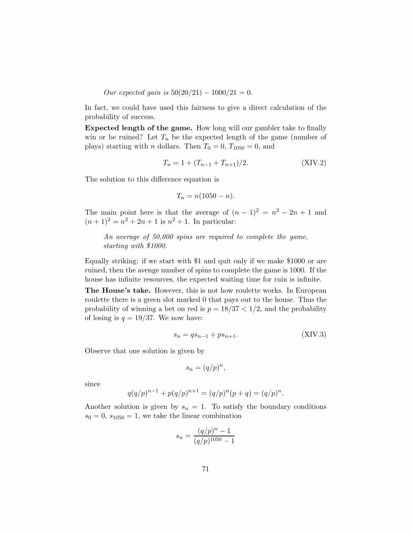
Our expected gain is 50(20/21) − 1000/21 = 0.
In fact, we could have used this fairness to give a direct calculation of theprobability of success.
Expected length of the game. How long will our gambler take to finallywin or be ruined? Let Tn be the expected length of the game (number ofplays) starting with n dollars. Then T0 = 0, T1050 = 0, and
Tn = 1 + (Tn−1 + Tn+1)/2. (XIV.2)
The solution to this difference equation is
Tn = n(1050 − n).
The main point here is that the average of (n − 1)2 = n2 − 2n + 1 and(n + 1)2 = n2 + 2n + 1 is n2 + 1. In particular:
An average of 50,000 spins are required to complete the game,starting with $1000.
Equally striking: if we start with $1 and quit only if we make $1000 or areruined, then the avenge number of spins to complete the game is 1000. If thehouse has infinite resources, the expected waiting time for ruin is infinite.
The House’s take. However, this is not how roulette works. In Europeanroulette there is a green slot marked 0 that pays out to the house. Thus theprobability of winning a bet on red is p = 18/37 < 1/2, and the probabilityof losing is q = 19/37. We now have:
sn = qsn−1 + psn+1. (XIV.3)
Observe that one solution is given by
sn = (q/p)n,
sinceq(q/p)n−1 + p(q/p)n+1 = (q/p)n(p + q) = (q/p)n.
Another solution is given by sn = 1. To satisfy the boundary conditionss0 = 0, s1050 = 1, we take the linear combination
sn =(q/p)n − 1
(q/p)1050 − 1
71
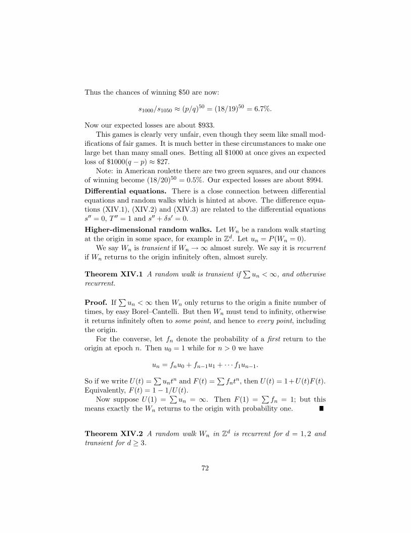
Thus the chances of winning $50 are now:
s1000/s1050 ≈ (p/q)50 = (18/19)50 = 6.7%.
Now our expected losses are about $933.This games is clearly very unfair, even though they seem like small mod-
ifications of fair games. It is much better in these circumstances to make onelarge bet than many small ones. Betting all $1000 at once gives an expectedloss of $1000(q − p) ≈ $27.
Note: in American roulette there are two green squares, and our chancesof winning become (18/20)50 = 0.5%. Our expected losses are about $994.
Differential equations. There is a close connection between differentialequations and random walks which is hinted at above. The difference equa-tions (XIV.1), (XIV.2) and (XIV.3) are related to the differential equationss′′ = 0, T ′′ = 1 and s′′ + δs′ = 0.
Higher-dimensional random walks. Let Wn be a random walk startingat the origin in some space, for example in Z
d. Let un = P (Wn = 0).We say Wn is transient if Wn → ∞ almost surely. We say it is recurrent
if Wn returns to the origin infinitely often, almost surely.
Theorem XIV.1 A random walk is transient if∑
un < ∞, and otherwiserecurrent.
Proof. If∑
un < ∞ then Wn only returns to the origin a finite number oftimes, by easy Borel–Cantelli. But then Wn must tend to infinity, otherwiseit returns infinitely often to some point, and hence to every point, includingthe origin.
For the converse, let fn denote the probability of a first return to theorigin at epoch n. Then u0 = 1 while for n > 0 we have
un = fnu0 + fn−1u1 + · · · f1un−1.
So if we write U(t) =∑
untn and F (t) =∑
fntn, then U(t) = 1+U(t)F (t).Equivalently, F (t) = 1 − 1/U(t).
Now suppose U(1) =∑
un = ∞. Then F (1) =∑
fn = 1; but thismeans exactly the Wn returns to the origin with probability one.
Theorem XIV.2 A random walk Wn in Zd is recurrent for d = 1, 2 and
transient for d ≥ 3.
72

Proof 1: the mathematician’s random walk. The proof is easy if wedefine a random walk in Z
d as a sum of independent random walks Sn(i) inZ, i.e. if we set
Wn = (Sn(1), Sn(2), . . . , Sn(d)) ∈ Zd.
Then we have un = 0 if n is odd, and
u2n = P (W2n = 0) = P (S2n(1) = 0)d ∼(
1√πn
)d
≍ 1
nd/2.
Since∑
n−d/2 < ∞ iff d ≥ 3, the preceding result completes the proof.
Proof 2: the physicist’s random walk. Alternatively one can define arandom walk in Z
d so it only changes one coordinate at a time; then eachstep is in one of 2d possible directions, with equal probability. For d = 1and d = 2 this is essentially the same as the walk above, so the analysis isthe same.
We now prove transience for d ≥ 3. For concreteness, assume d = 3.Then we have
u2n = 6−2n∑ (2n)!
i!i!j!j!k!k!,
where the sum is over all partitions i + j + k = n. We can rewrite this as
u2n = 2−2n
(2n
n
)∑(3−n n!
i!j!k!
)2
.
The terms which are squared come from the trinomial distribution, so theirsum is no bigger than the largest term, which occurs when i, j and k are allabout n/3. In other words, we have
u2n = O
(1√n
n!
3n((n/3)!)3
).
Now by Stirling’s formula, we have n! ≍ √n(n/e)n and hence (3n(n/3)!)3 ≍
n3/2(n/e)n. This gives u2n = O(1/n3/2), so∑
u2n < ∞.
Coda: The paradox of bad luck. Here are two paradoxes showing thepersistence of bad luck (cf. Feller Volume 2, Ch. I.), also based on divergentseries.
73

1. Suppose parking tickets are given out at random. At the end of theyear, how many neighbors will I need to consult to find one who gotmore tickets than me? All things being equal, in a group of n I have a1/n chance of having the most tickets. Since
∑1/n = ∞, on average
it will take forever to find a neighbor with worse luck. (The expectedwaiting time for first success is
∑qn, where qn is the probability of
failure in the first n trials.)
2. Suppose you are in a traffic jam on 2-lane highway. It is impossible tochange lanes. Every now and then, the right or left lane advances byone car. Each lane has the same chance of advancing.
The red car next to you moves up one. How long do you expect it willtake for you to catch up?
This is the same as the waiting time for a first return to the origin ina random walk: it is infinite.
The red car’s driver hopes to eventually get two lengths ahead of you.However, his expected waiting time for this event is also infinite. Andnevertheless, the gap between the two of you eventually gets arbitrarilylarge.
To clarify the paradox — note that there is a big difference betweensaying the expected waiting time is infinite, and that you should expectto wait an infinite amount of time. In fact, you are certain to eventuallypass the red car, and get as large a lead as you might wish.
Keep in mind that any event which has the slightest positive chanceof never happening has an expected waiting time of infinity. A singleimmortal vampire makes the average lifetime infinite.
74
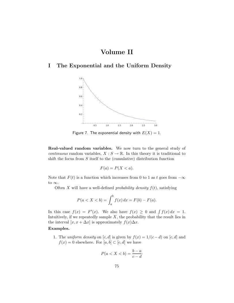
Volume II
I The Exponential and the Uniform Density
0.5 1.0 1.5 2.0 2.5 3.0
0.2
0.4
0.6
0.8
1.0
Figure 7. The exponential density with E(X) = 1.
Real-valued random variables. We now turn to the general study ofcontinuous random variables, X : S → R. In this theory it is traditional toshift the focus from S itself to the (cumulative) distribution function
F (a) = P (X < a).
Note that F (t) is a function which increases from 0 to 1 as t goes from −∞to ∞.
Often X will have a well-defined probability density f(t), satisfying
P (a < X < b) =
∫ b
af(x) dx = F (b) − F (a).
In this case f(x) = F ′(x). We also have f(x) ≥ 0 and∫
f(x) dx = 1.Intuitively, if we repeatedly sample X, the probability that the result lies inthe interval [x, x + ∆x] is approximately f(x)∆x.
Examples.
1. The uniform density on [c, d] is given by f(x) = 1/(c− d) on [c, d] andf(x) = 0 elsewhere. For [a, b] ⊂ [c, d] we have
P (a < X < b) =b − a
c − d·
75
The distribution function F (t) increases linearly from F (c) = 0 toF (d) = 1. Clearly E(X) = (c + d)/2.
2. For α > 0, the exponential density is given by
f(x) = α exp(−αx)
on [0,∞). We have F (t) = 1 − exp(−αt) for t ≥ 0.
3. A single Bernoulli trial X has the distribution function F (t) = 0 fort ≤ 0, F (t) = q in (0, 1], and F (t) = 1 for t > 1. Its ordinary derivativedoes not exist, but it is conventional to write
F ′(t) = qδ0 + pδ1.
4. In the same way a discrete random variable with probability distribu-tion pk has
F (t) =∑
k<t
pk and f(t) =∑
k
pkδk.
5. The normal distribution is given f(x) = n(x) = (2π)−1/2 exp(−x2/2).
6. The arcsine law is given by the density f(x) = (πx(1 − x))−1/2, withdensity F (x) = (2/π) arcsin(
√x) on [0, 1].
What are the events? Here is a technical problem we are skirting. Sup-pose X is chosen uniformly at random in the interval [0, 1]. Then for ‘any’A ⊂ [0, 1] we have
P (X ∈ A) = |A|.But what is |A|? For an interval this is clear, but what about for a moregeneral subset of [0, 1]?
It turns out to be a technical challenge to identify exactly the sets forwhich the event X ∈ A has a well-defined probability. A full resolutionrequires the theory of Lebesgue measure. Luckily we can skirt this issuefor now! (As a warmup, one might ask: what is the probability that X isrational?)
From the discrete to the continuous. Continuous random variablesemerge frequently as limits of discrete random variables. To make this pre-cise, let us say (the distribution of) a random variable Xn converges to (thatof) X if, for each a ∈ R, we have
P (X < a) = lim P (Xn < a).
76
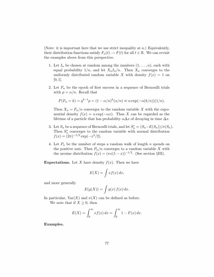
(Note: it is important here that we use strict inequality at a.) Equivalently,their distribution functions satisfy Fn(t) → F (t) for all t ∈ R. We can revisitthe examples above from this perspective.
1. Let In be chosen at random among the numbers (1, . . . , n), each withequal probability 1/n, and let XnIn/n. Then Xn converges to theuniformly distributed random variable X with density f(x) = 1 on[0, 1].
2. Let Fn be the epoch of first success in a sequence of Bernoulli trialswith p = α/n. Recall that
P (Fn = k) = qk−1p = (1 − α/n)k(α/n) ≈ α exp(−α(k/n))(1/n).
Then Xn = Fn/n converges to the random variable X with the expo-nential density f(x) = α exp(−αx). Thus X can be regarded as thelifetime of a particle that has probability α∆x of decaying in time ∆x.
3. Let Sn be a sequence of Bernoulli trials, and let S∗n = (Sn−E(Sn))/σ(Sn).
Then S∗n converges to the random variable with normal distribution
f(x) = (2π)−1/2 exp(−x2/2).
4. Let Pn be the number of steps a random walk of length n spends onthe positive axis. Then Pn/n converges to a random variable X withthe arcsine distribution f(x) = (πx(1 − x))−1/2. (See section §III).
Expectations. Let X have density f(x). Then we have
E(X) =
∫xf(x) dx,
and more generally
E(g(X)) =
∫g(x) f(x) dx.
In particular, Var(X) and σ(X) can be defined as before.We note that if X ≥ 0, then
E(X) =
∫ ∞
0xf(x) dx =
∫ ∞
01 − F (x) dx.
Examples.
77
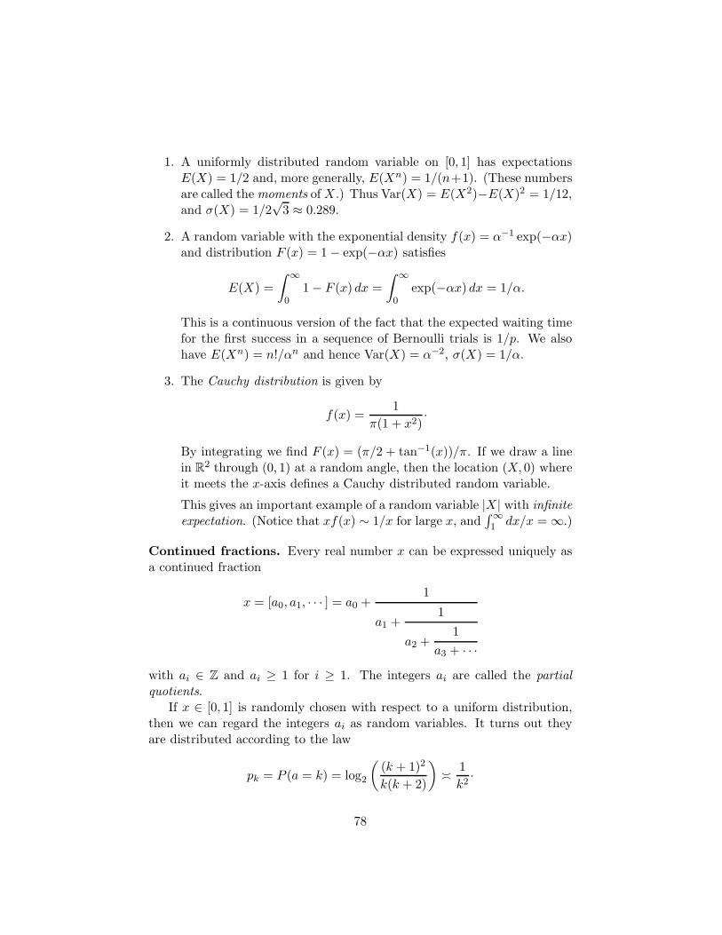
1. A uniformly distributed random variable on [0, 1] has expectationsE(X) = 1/2 and, more generally, E(Xn) = 1/(n+1). (These numbersare called the moments of X.) Thus Var(X) = E(X2)−E(X)2 = 1/12,and σ(X) = 1/2
√3 ≈ 0.289.
2. A random variable with the exponential density f(x) = α−1 exp(−αx)and distribution F (x) = 1 − exp(−αx) satisfies
E(X) =
∫ ∞
01 − F (x) dx =
∫ ∞
0exp(−αx) dx = 1/α.
This is a continuous version of the fact that the expected waiting timefor the first success in a sequence of Bernoulli trials is 1/p. We alsohave E(Xn) = n!/αn and hence Var(X) = α−2, σ(X) = 1/α.
3. The Cauchy distribution is given by
f(x) =1
π(1 + x2)·
By integrating we find F (x) = (π/2 + tan−1(x))/π. If we draw a linein R
2 through (0, 1) at a random angle, then the location (X, 0) whereit meets the x-axis defines a Cauchy distributed random variable.
This gives an important example of a random variable |X| with infiniteexpectation. (Notice that xf(x) ∼ 1/x for large x, and
∫∞1 dx/x = ∞.)
Continued fractions. Every real number x can be expressed uniquely asa continued fraction
x = [a0, a1, · · · ] = a0 +1
a1 +1
a2 +1
a3 + · · ·
with ai ∈ Z and ai ≥ 1 for i ≥ 1. The integers ai are called the partialquotients.
If x ∈ [0, 1] is randomly chosen with respect to a uniform distribution,then we can regard the integers ai as random variables. It turns out theyare distributed according to the law
pk = P (a = k) = log2
((k + 1)2
k(k + 2)
)≍ 1
k2·
78
For example, p1 = log2(4/3) ≈ 0.415, p2 = log2(9/8) ≈ 0.16, etc. Inparticular, the expected value of the partial quotients is infinite!
Note that large values of ai correspond to good rational approximationsto x. For example, the continued fraction of π is given by
π = [3, 7, 15, 1, 292, 1, 1, 1, 2, 1, 3, 1, 14, 2, . . .]
We have π ≈ [3, 7] = 3 + 1/7 = 22/7, but even better π ≈ [3, 7, 15, 1] =355/113 ≈ 3.1415929; this last is quite good because the partial quotient292 is so large.
The continued fraction of π appears to have the same statistics as arandom point, but it has not even been proved that the ai’s for π are un-bounded.
Independent variables and convolution. We say X and Y are inde-pendent if for all a, b, c, d we have
P (a < X < b and c < Y < d) = P (a < X < b) · P (c < Y < d).
The definition for more than two random variables is analogous.If X1 and X2 are independent with densities f1(x) and f2(x), then the
density of X = X1 + X2 is given by the convolution
f(a) =
∫f1(x)f2(a − x) dx = (f1 ∗ f2)(a).
This follows from the fact that its distribution function satisfies
F (a) = P (X < a) =
∫
x1+x2<af1(x1)f2(x2) dx1 dx2 =
∫F1(x)f2(a − x) dx.
In both cases the result is symmetric in X1 and X2.One should compare f1 ∗ f2 to the product of generating functions in the
case of discrete random variables.
Uniform and exponential examples. If X1 and X2 have a uniformdistribution, then X = X1 + X2 has distribution
f(x) = min(x, 2 − x), x ∈ [0, 2].
Thus F (t) = P (X < t) = t2/2 for t ∈ [0, 1], and 1 − t2/2 for t ∈ [1, 2]. Notethat F (t) is simply the area of the intersection of the unit square [0, 1]×[0, 1]with the region x1 + x2 ≤ t.
79
If X1 and X2 have the same exponential density α exp(−αs), then X =X1 + X2 has the density
f(s) =
∫ s
0α2 exp(−αt) exp(αt − αs) dt = α2s exp(−αs).
Notice that f(0) = 0 every thought f1(0) = f2(0) = 1.
Ratios of variables. It also straightforward to compute the distributionof the ratio X = X1/X2 of two non-negative, independent random variableswith densities f1(x) and f2(x). Indeed, since
G(t) = P (X < t) = P (X1 < tX2) =
∫ ∞
0f2(x)F1(tx) dx,
the density of X is given by
g(t) = G′(t) =
∫ ∞
0xf2(x)f1(tx) dx.
If X and 1/X have the same distribution, then we also have
g(t) = t−2g(1/t).
Examples. (i) If X1 and X2 are chosen uniformly in [0, 1], then for t ≤ 1we have g(t) = 1/2, and for t > 1 we have g(t) = 1/(2t2). (ii) If X1 and X2
have an exponential distribution (with any α), then
g(t) =
∫ ∞
0α2x exp(−α(1 + t)x) dx = (1 + t)−2,
and 1 − G(t) = 1/(1 + t). Thus when two people stand in the same line,half the time one has to wait 3 or more times longer than the other (sinceP (X1/X2 > 3) = 1 − G(3) = 1/4.
Moreover, in both examples, E(X1/X2) is infinite. This is a commonphenomenon; it arises just because E(1/X2) is infinite. Indeed, if the densityf(x) has a positive limit f(0) as x → 0+, then E(1/X) = ∞. To see this,note that the distribution function of Y = 1/X is given by
P (Y < t) = P (X > 1/t) = 1 − F (1/t),
so the density of Y is given by
g(t) = f(1/t)/t2,
80
and if f(1/t) → c 6= 0 as t → ∞, then
E(Y ) =
∫tg(t)dt ≈
∫ ∞
1ct/t2 dt = ∞.
If X1 is not identically zero, then P (X1 > a) > 0 for some a, and thusE(X1/X2) ≥ P (X1 > a)E(a/X2) = ∞.
More on exponentially distributed random variables. We now turnto a more detailed discussion of a random variable X with the exponentialdistribution,
f(x) = α exp(−αx), F (x) = 1 − exp(−αx);
note that F ′(x) = f(x). Here are some of the ways it arises naturally.
1. The function L(s) = P (X > s) = 1 − F (s) satisfies the importantrelation:
L(s + t) = L(s)L(t)
for all s, t > 0, and is indeed characterized by this relation. If we thinkof X as the length of a lifetime, this means the probability of survivingfor time s + t is the probability of first surviving for time s and thensurviving for an additional time t. The essential feature is that therisk of death is always the same, and the threats at different times areindependent.
Note that the expected lifetime is E(X) = 1/α.
2. The probability that a thread of length t can sustain a fixed loadsatisfies P (t + s) = P (t)P (s). So the length X at which the threadsnaps is an exponentially distributed random variable.
3. The exponential distribution arises as the limit of the waiting time forfirst success in a sequence of Bernoulli trials with probability p → 0,with n → ∞ trials in each unit time interval, and with np → α. Notethat α is the expected number of successes in a unit time interval.In the survival model this is the expected number of fatalities, whichexplains why the expected lifetime is 1/α.
In the discrete case, the epoch of first success is exponentially dis-tributed, with
pk = qk−1p.
81

If we let x = k/n, then ∆x = 1/n = p/α, and we have
pk ∼ (1 − p)kp = (1 − α/n)nxα∆x → αe−αx∆x
as n → ∞.
4. The Poisson process with density λ produces a random set A ⊂ [0,∞)with E(|A ∩ [a, b]) = λ|b − a|). We have seen that
P (|A ∩ I| = k) = exp(−λ|I|)λk|I|kk!
·
This implies the location X ≥ 0 of the smallest point in A is exponen-tially distributed: we have
P (X > t) = P (A ∩ [0, t] = ∅) = exp(−λt).
Since the Poisson process is a limit of Bernoulli trials, it is no surprisethat the location of its smallest point is a limit of the waiting time forthe first success.
5. The gaps between consecutive points in the Poisson process have thesame distribution as the smallest point; they are also exponentiallydistributed, with the expected gap size 1/λ.
6. Fire a rifle in a thin forest, and let X be the distance the bullet travelsbefore hitting a tree. Then X is exponentially distributed (to a goodapproximation).
Indeed, we can model the trees in the forest by a collection of disks ofradius r in the plane whose centers are chosen using a Poisson processof density λ. (Some disks may overlap, but this is unlikely if the forestis thin, i.e. if λr2 is small.)
If our bullet travels distance ≥ t then there are no centers withindistance r of a given line of length t. The area of this region being 2rt,we find
P (X > t) = exp(−2λrt)
by the definition of the Poisson process.
7. By the same token, the distance X between a tree and its nearestneighbor satisfies
P (X > t) = exp(−λπt2),
since the event X > t requires a region of area πt2 to be free of trees.(Here our idealized trees have r = 0.)
82
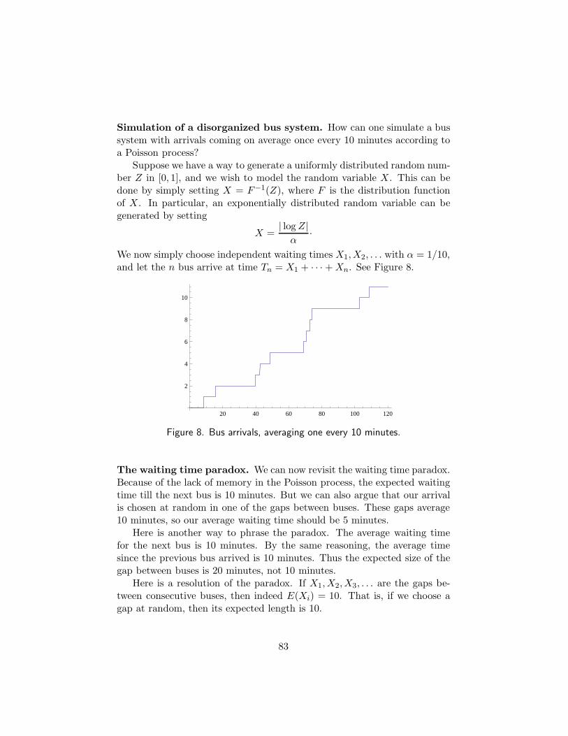
Simulation of a disorganized bus system. How can one simulate a bussystem with arrivals coming on average once every 10 minutes according toa Poisson process?
Suppose we have a way to generate a uniformly distributed random num-ber Z in [0, 1], and we wish to model the random variable X. This can bedone by simply setting X = F−1(Z), where F is the distribution functionof X. In particular, an exponentially distributed random variable can begenerated by setting
X =| log Z|
α·
We now simply choose independent waiting times X1,X2, . . . with α = 1/10,and let the n bus arrive at time Tn = X1 + · · · + Xn. See Figure 8.
20 40 60 80 100 120
2
4
6
8
10
Figure 8. Bus arrivals, averaging one every 10 minutes.
The waiting time paradox. We can now revisit the waiting time paradox.Because of the lack of memory in the Poisson process, the expected waitingtime till the next bus is 10 minutes. But we can also argue that our arrivalis chosen at random in one of the gaps between buses. These gaps average10 minutes, so our average waiting time should be 5 minutes.
Here is another way to phrase the paradox. The average waiting timefor the next bus is 10 minutes. By the same reasoning, the average timesince the previous bus arrived is 10 minutes. Thus the expected size of thegap between buses is 20 minutes, not 10 minutes.
Here is a resolution of the paradox. If X1,X2,X3, . . . are the gaps be-tween consecutive buses, then indeed E(Xi) = 10. That is, if we choose agap at random, then its expected length is 10.
83

But if we choose a time at random, then we are more likely to land ina large gap than a small gap. That is, the probability of landing in a gapof size x should be proportional to the product of the length of the gap andthe probability that a gap of that size occurs. So if we sample by randomtimes, the gap size Y is distributed according to the density
g(y) = α2y exp(−αy).
The constant α2 is determined by the fact that∫
g(y) dy = 1.Notice that g is exactly the convolution f ∗ f for f(x) = α exp(−αx)
computed above. In other words, Y is distributed as the sum X1 + X2 oftwo exponential waiting times with E(Xi) = 10. In particular E(Y ) = 20.Its behavior is consistent with our reasoning that the length of time betweenbuses is the sum of the time to the next bus and the time from the precedingbus.
Thus the paradox arises from ambiguity in the notion of a randomlychosen gap.
Completion of a task. Suppose an order for a new passport must passconsecutively through n independent levels of administration, each takingon average time 1/α to complete their review. What is the distribution ofthe total time Sn = X1 + · · · + Xn required to get the passport back?
We may assume Xi has the distribution f(x) = α exp(−αx), in whichcase we need only compute the n-fold convolution fn(x) = (f ∗f ∗· · ·∗f)(x).This can be done inductively, and we find
fn(x) = α(αx)n−1
(n − 1)!exp(−αx).
The case n = 2 was considered above. We have E(Sn) = n/α and Var(Sn) =n/α2. By the central limit theorem, S∗
n limits to a normal distribution; equiv-alently, when suitably rescaled, the graph of the function xne−x approachesa bell curve.
Order statistics: the exponential post office. The zip code 27182is served by a post office with n windows, each staffed by an exponential,independent worker who serves on average α customers per hour. Thismeans the time Xi to service a customer at the ith window has the densityf(x) = α exp(−αx).
Suppose when you arrive at the post office, each window is occupied byexactly one customer. No more customers are expected for the day.
1. How long will it take for a free window to open up?
84

The answer is X(1) = min(X1, . . . ,Xn). This variable has the distribu-tion f1(x) = nα exp(−nαx). To see this, recall that Xi is essentiallya waiting time for a first success. Thus X(1) is also a waiting time forfirst success, but with trials proceeding n times faster.
For a proof based on calculation, just note that
P (X(1) > t) =n∏
1
P (Xi > t) = exp(−nαt).
Note: the Markov property (lack of memory) for the variables Xi
means the amount of time a customer has already spent at the windowhas no effect on how long it will take for him to finish.
2. What are the chances I will be the last person to leave the post office?
The answer is 1/n. Once a window opens up, all the customers aretreated equally, again by the Markov property.
3. Suppose I simply want to wait until all the customers leave, so I canrob the post office (take all their stamps). How long should I expectto wait?
Let X(i) be the time it takes for a total of i customers to be serviced.We have already seen that X(1) has an exponential distribution withconstant nα. By the Markov property, X(k) −X(k−1) has an exponen-tial distribution with constant (n − k)α. Hence
E(X(n)) =1
α
(1
n+
1
n − 1+ · · · 1
1
)≈ log n
α·
Note that the expected time required to service n customers at 1 win-dow is n/α. Serving n customers with n windows is less efficient,because many windows are idle while the last few customers are beingserved.
4. What is the distribution of the time X(k) required for k of the n cus-tomers to be serviced? The event X(k) < t means that k or more ofthe events (Xi < t) occur. Hence
Fk(t) = P (X(k) < t) =
n∑
j=k
(n
j
)(1 − exp(−αt))j exp(−αt)n−j .
85
By differentiating, one finds the density of X(k) is given by:
fk(t) = n
(n − 1
k − 1
)(1 − exp(−αt))k−1 exp(−αt) exp(−αt)n−k.
This formula can be easily seen directly. If X(k) is in the interval[t, t + ∆t], this means (k − 1) customers have already finished, a kthcustomer finished in this interval, and the remaining (n−k) customersare taking longer. This partition of n into 3 sets can be made in n
(n−1k−1
)
ways. For each partition, the probability that the chosen (k − 1)customers have left is given by the first term in the product above,and the probability that the remaining (n − k) customers are stillwaiting is given by the last term. The middle term, times ∆t, givesthe probability that the one remaining customer leaves during the timeinterval [t, t + ∆t].
Radioactive decay. It is common to measure the rate of decay of anunstable particle by its half life T . This is the median decay time, i.e. it isthe solution to exp(−αT ) = 1/2, namely T = log 2/α. (The expected timeto decay is longer, namely 1/α.)
Thus the expected time for a sample of n atoms to decay completely isgiven by
E(X(n)) =log n
α= T log2 n
This is intuitively clear — if the half the sample decays in time T , then thenumber of atoms left after time kT is 2−kn.
Example: Iodine 131 has a half-life of 8.02 days. (It mostly undergoesbeta decay, in which a neutron emits an electron to become a proton, re-sulting in stable xenon). The mass of a single atom is about 131 u, whereu = 1.66 × 10⁻²⁴g. Thus a gram of I-131 contains about n = 4.6 × 10²¹
atoms; we have log2 n ≈ 72, and hence it takes about 577 days to decaycompletely.
Of course a very small sample of I-131 poses little health risk. The samecannot be said for a small number of bacteria or infested plants. Recall thecrop-duster analysis of Ch. IV.
The two envelopes problem.
The two envelopes problem is a puzzle or paradox within the sub-jectivistic interpretation of probability theory; more specificallywithin subjectivistic Bayesian decision theory. This is still an
86
open problem among the subjectivists as no consensus has beenreached yet.
—Wikipedia, 4/2011.
Here is a variant of the Monty Hall paradox. Two envelopes hold 10 and 20dollars respectively. You are presented with one at random. Would you liketo switch to the other?
Of course it makes no difference. Your expected payoff is 15 in eithercase.
Now suppose you are told that one envelope holds twice as much as theother. You open the first envelope and find X dollars. If you switch, youwill get either X/2 or 2X dollars. Since the average of these is 5X/4, ofcourse you should switch (?).
One way to clarify the paradox is this. There are indeed two possibilities;the envelope you hold contains C dollars, and the other contains D = 2Cor D = C/2. But more precisely, D = 2C when C = 10 and D = C/2 whenC = 20. It is a mistake to assume that D/C is independent of C!
Now let’s make the problem more precise and devise a reasonable strat-egy. Let us suppose the envelopes hold A and B = 2A dollars, where A is arandom variable with finite expectation. Let us also suppose you know thedistribution of A, and the value C in the first envelope.
In this case, one can sometimes give a good reason for switching. Forexample, if A is always odd, then you should switch whenever C is odd.
To handle the general case, we suppose A is chosen at random on R withrespect to the density f(x), that K is a Bernoulli trial with values 1 or 2with equal probability, and that A and K are independent. Then C = AK.
Suppose we switch envelopes when C ∈ E. Then we gain A if K = 1 (inwhich case A = C ∈ E), but we lose A if K = 2 (in which case A = C/2 ∈E/2). Thus our expected gain is
g =1
2
(∫
Exf(x) dx −
∫
E/2xf(x)
)dx.
Now if E = [s, s + ∆s], then
2g ≈ sf(s)∆s − (s/2)f(s/2)∆s/2 > 0
iff f(s) ≥ f(s/2)/4. So we should switch if
C ∈ E = {s : 4f(s) > f(s/2)}.
87
Example: for the uniform distribution on [0, 1], we should switch if C ∈ [0, 1],but not switch if C ∈ [1, 2]. (Of course in the latter case we know we holdthe envelope containing 2A.)
For an exponential distribution f(s) = α exp(−αs), we should switchwhen
C < (4 log 2)/α = (4 log 2)E(A) ≈ 2.772E(A).
This is an example of optimal decision–making guided by probabilitytheory.1
Optimal stopping times. Here is another classical optimization problem.In this year n movies will be released. Your goal is to pick the best movie ofthe year the moment it comes out (to seal your reputation as a reviewer).
The outcome is considered a success only if you correctly pick the bestmovie. You get no credit for picking second largest.
What strategy should you pursue to maximize the probability of success?And what is your probability of success, for large n?
Let us assume the movies have already been made, and the ith moviethat is released has quality Xi (an objective amount), but otherwise nothingis known except the total number that will be released.
It turns out that any optimal strategy must have the following form:
Reject the first s movies, then select the first movie that is betterthan any you have seen so far. mbut record that highest quality
As an example, let s = n/2. Then if X(2) = Xi for i ∈ [1, s] while themaximum X(1) = j occurs for j ∈ [s + 1, n], then the strategy will success.These events are independent and each has probability 1/2, so s = n/2 hasa success rate for 1/4.
To analyze the success rate for general s, suppose the maximum occursat index k ∈ [1, n]. All these indices are equally likely, and we certain fail ifk ≤ s. What about for k > s? To succeed then, we need that:
The maximum of (X1, . . . ,Xk−1) occurs at an index i ≤ s.
For if it occurs at an index i ∈ [s + 1, k − 1], we will acccept this ‘falsemaximum’ as our final result. But otherwise we will wait until Xk.
Now the probability of the event above is just s/(k − 1), again becauseeach of the indices in [1, k−1] are equally likely. So the probability of success
1Here is another envelope problem: suppose you do not know the distribution of the
amount placed in the envelopes. Devise a strategy for switching which does better, on
average, than never switching at all.
88
is:
p(s) =1
n
n∑
k=s+1
s
k − 1≈ s
n
∫ n
s
dx
dx=
s
nlog
n
s·
The function f(x) = x log(1/x) has f ′(x) = log(1/x) − 1 = 0 at x = 1/e,where it assumes the value f(1/e) = 1/e.
Thus the optimal strategy is to reject the first ≈ n/e ≈ 0.368nnumbers, and then accept the next record breaker.
The success rate is similarly 1/e ≈ 36.8%. Note that there are two types offailure: finding no new record, and accepting a new record that is still notoptimal. The first type only happens when the maximum value of Xi occursin the interval [1, s], so its probability is also s/n ≈ 1/e. A false maximumis chosen the rest of the time, i.e. in 1 − 2/e = 26.4% of the cases.
More on uniformly distributed random variables. When one speaksof a point X chosen at random in [0, 1], this usually means chosen at randomwith respect to the uniform density. That is, P (X ∈ A) = |A| for anyinterval A ⊂ [0, 1].
A sequence of independent, uniformly distributed random variables
(X1, . . . ,Xn) ∈ [0, 1]n
is the same as a random point in a cube. Such a sequence cuts [0, 1] into(n + 1) intervals, [0,X(1)], [X(1),X(2)], · · · [X(n), 1]. As before, the orderstatistics (X(1), . . . ,X(n)) are obtained by putting the sequence (X1, . . . ,Xn)into increasing order.
Theorem I.1 The lengths (L1, . . . , Ln+1) of the complementary intervalsX(1), X(2) − X(1), . . ., 1 − X(n) have a common distribution, satisfying:
1 − Fn(t) = P (Li > t) = (1 − t)n and fn(t) = n(1 − t)n−1.
The expected length of a complementary interval is 1/(n + 1).
Proof. Imagine instead that we choose (n + 1) independent points, uni-formly distributed on the unit circle S1 = R/Z. It is then clear that all thegaps have the same distribution.
To compute the value of 1 − F (t), we just note that the condition L1 =X(1) = min(X1, . . . ,Xn) > t means that each Xi lies in the interval (t, 1],and the volume of the subcube (t, 1)n in [0, 1]n is (1 − t)n. Since
∑Li = 1,
we have E(Li) = 1/(n + 1).
89

Corollary I.2 The expected value of X(k) is k/(n + 1).
Proof. E(X(k)) = E(∑k
1 Li
).
Theorem I.3 The order statistics X(k) for a uniform distribution of npoints in [0, 1] have densities
fk(t) = n
(n − 1
k − 1
)tk−1(1 − t)n−k.
Proof. This is similar to the exponential case: to get X(k) in [t, t + ∆t] weneed to have k − 1 points with Xi < t; if their indices are fixed, then theprobability of this event in tk−1. We also need n − k points in [t, 1]; thiscontributes a factor of (1 − t)n−k. The one remaining point must land in[t, t + ∆]; the probability of this event is ∆t. Finally the number of ways ofpartitioning n into these three sets is n
(n−1k−1
).
Note that fk(t)/n is exactly the probability that among n− 1 Bernoullitrials of probability t, we have k − 1 successes.
Correlation. Unlike the order statistics for the exponential distribution,the lengths L1, . . . , Ln+1 are correlated, as can be seen immediately from thefact that Var(
∑Li) = 0. For example, when n = 1, we have L2 = 1 − L1,
and hence ρ(L1, L2) = −1.
The uniform post office. In the uniform post office, the service timerequired at the ith window is a uniformly distributed random variable in[0, 1]. As before, each window has exactly one customer when I arrive.
1. What is the expected wait for a free window to open up? This isE(X(1)) = E(L) = 1/(n + 1).
2. How long will it take, on average, for all customers n to be serviced?Answer: E(X(n)) = n/(n + 1).
3. Suppose we have n = 2k − 1 windows. How is the departure time ofthe middle customer, X(k), distributed?
Answer: it behaves like a normally distributed random variable withE(X) = 1/2 and σ(X) = 1/(2
√n). Indeed, if t = 1/2 + s, then the
density fk(t) is a constant multiple of
(1 + 2s)k(1 − 2s)k = (1 − 4s2)k =
(1 − 4ks2
k
)k
∼ exp(−4ks2) = exp(−s2/2σ2),
90

where σ2 = 1/8k ≈ 1/4n.
Roulette, Benford’s law and the uniform distribution. The numberof total turns T of a roulette will be fairly smoothly distributed over a largeinterval [0,M ]. The outcome of the game is given by the random variableX = T mod1. It is easy to believe, and not hard to prove, that X will beclose to uniformly distributed if M is large and the distribution is smoothenough. For example, if the density g(t) of T is increasing for t < a anddecreasing for t > a, and f(a) = m, then the density f(x) of X satisfies|f(x)−1| ≤ m. This is because f(x) =
∑n g(x+n) is a good approximation
to∫
g(t) dt = 1.By the same token, for any random variable T with a large range (many
orders of magnitude) and rather smooth distribution, X = log10 T mod 1will be approximately uniformly distributed. But the value of the first digitN of T depends only on X; this gives rise to Benford’s law:
P (N = k) =log(k + 1) − log k
log 10·
Thus P (N = 1) = log10 2 ≈ 30.1%, while P (N = 9) = 1 − log10 9 ≈ 4.6%.
Random directions; other densities. Suppose X has the density f(x)and X = φ(Y ), where φ is 1 − 1. Then the density g(y) of Y is given by
g(y) = f(φ(y))|φ′(y)|.
This is intuitively clear: if Y is [y, y+∆y], then X is in [φ(y), φ(y)+φ′(y)∆y]and the probability of the latter event is f(φ(y))|φ′(y)|∆y. It can also beseen using distribution functions. If φ is increasing, then
G(t) = P (Y < t) = P (X < φ(t)) = F (φ(t)),
so g′(t) = f(φ(t))φ′(t).In particular, if X is uniformly distributed, then g(y) = φ′(y). For
example, if X is chosen uniform in [−1/2, 1/2], and Y = tan(πX), thenX = (1/π) tan−1(Y ) and hence g(y) = 1/(π(1 + y2)). This is the source ofthe Cauchy distribution.
Theorem I.4 The tangent of a random angle is distributed according to theCauchy density f(x) = 1/(π(1 + x2)).
Projections.
91
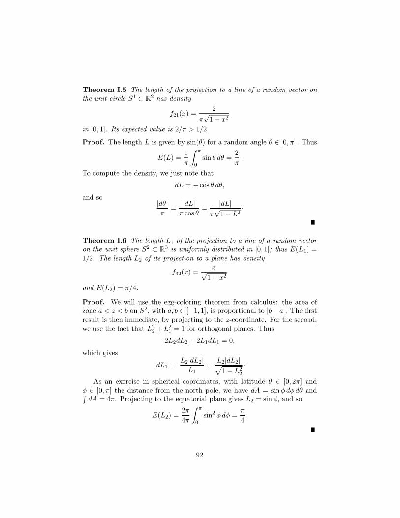
Theorem I.5 The length of the projection to a line of a random vector onthe unit circle S1 ⊂ R
2 has density
f21(x) =2
π√
1 − x2
in [0, 1]. Its expected value is 2/π > 1/2.
Proof. The length L is given by sin(θ) for a random angle θ ∈ [0, π]. Thus
E(L) =1
π
∫ π
0sin θ dθ =
2
π·
To compute the density, we just note that
dL = − cos θ dθ,
and so|dθ|π
=|dL|
π cos θ=
|dL|π√
1 − L2·
Theorem I.6 The length L1 of the projection to a line of a random vectoron the unit sphere S2 ⊂ R
3 is uniformly distributed in [0, 1]; thus E(L1) =1/2. The length L2 of its projection to a plane has density
f32(x) =x√
1 − x2
and E(L2) = π/4.
Proof. We will use the egg-coloring theorem from calculus: the area ofzone a < z < b on S2, with a, b ∈ [−1, 1], is proportional to |b−a|. The firstresult is then immediate, by projecting to the z-coordinate. For the second,we use the fact that L2
2 + L21 = 1 for orthogonal planes. Thus
2L2dL2 + 2L1dL1 = 0,
which gives
|dL1| =L2|dL2|
L1=
L2|dL2|√1 − L2
2
·
As an exercise in spherical coordinates, with latitude θ ∈ [0, 2π] andφ ∈ [0, π] the distance from the north pole, we have dA = sin φdφdθ and∫
dA = 4π. Projecting to the equatorial plane gives L2 = sin φ, and so
E(L2) =2π
4π
∫ π
0sin2 φdφ =
π
4.
92
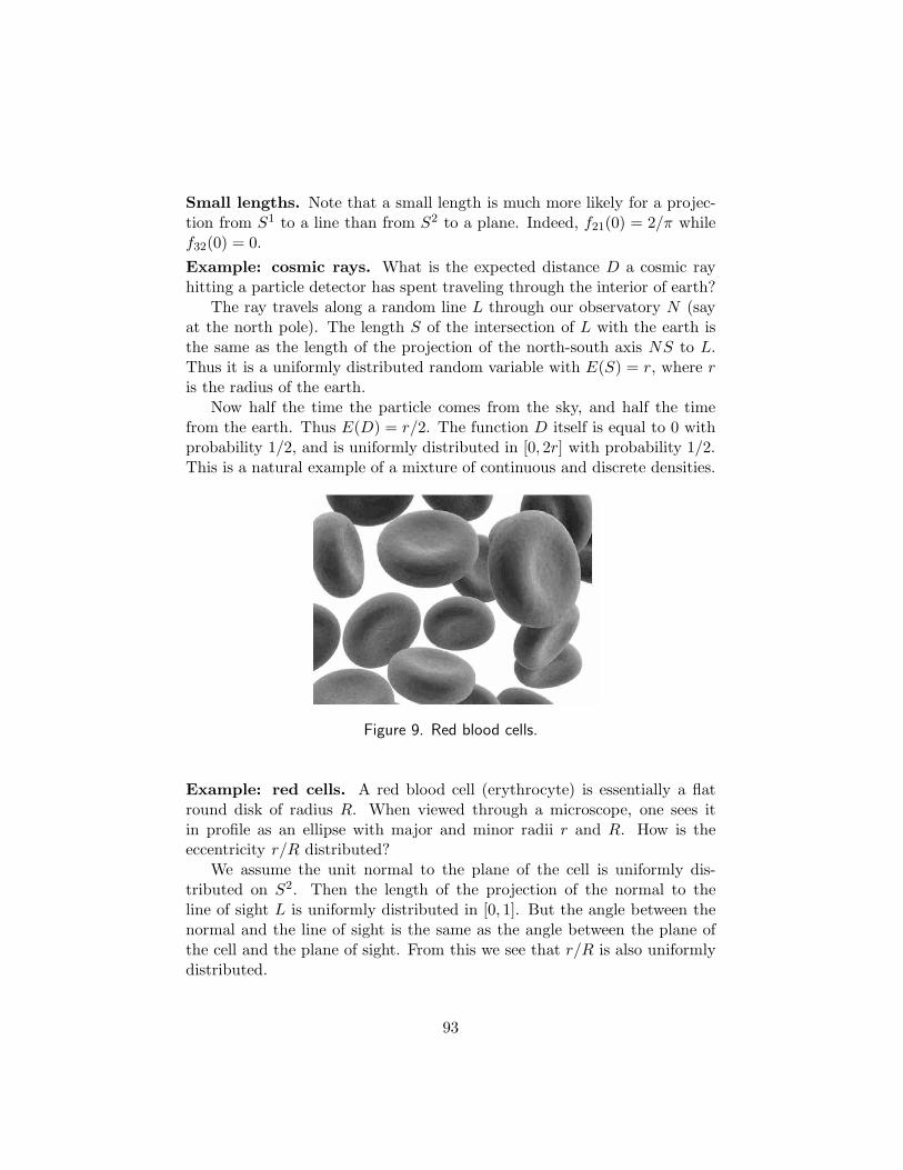
Small lengths. Note that a small length is much more likely for a projec-tion from S1 to a line than from S2 to a plane. Indeed, f21(0) = 2/π whilef32(0) = 0.
Example: cosmic rays. What is the expected distance D a cosmic rayhitting a particle detector has spent traveling through the interior of earth?
The ray travels along a random line L through our observatory N (sayat the north pole). The length S of the intersection of L with the earth isthe same as the length of the projection of the north-south axis NS to L.Thus it is a uniformly distributed random variable with E(S) = r, where ris the radius of the earth.
Now half the time the particle comes from the sky, and half the timefrom the earth. Thus E(D) = r/2. The function D itself is equal to 0 withprobability 1/2, and is uniformly distributed in [0, 2r] with probability 1/2.This is a natural example of a mixture of continuous and discrete densities.
Figure 9. Red blood cells.
Example: red cells. A red blood cell (erythrocyte) is essentially a flatround disk of radius R. When viewed through a microscope, one sees itin profile as an ellipse with major and minor radii r and R. How is theeccentricity r/R distributed?
We assume the unit normal to the plane of the cell is uniformly dis-tributed on S2. Then the length of the projection of the normal to theline of sight L is uniformly distributed in [0, 1]. But the angle between thenormal and the line of sight is the same as the angle between the plane ofthe cell and the plane of sight. From this we see that r/R is also uniformlydistributed.
93
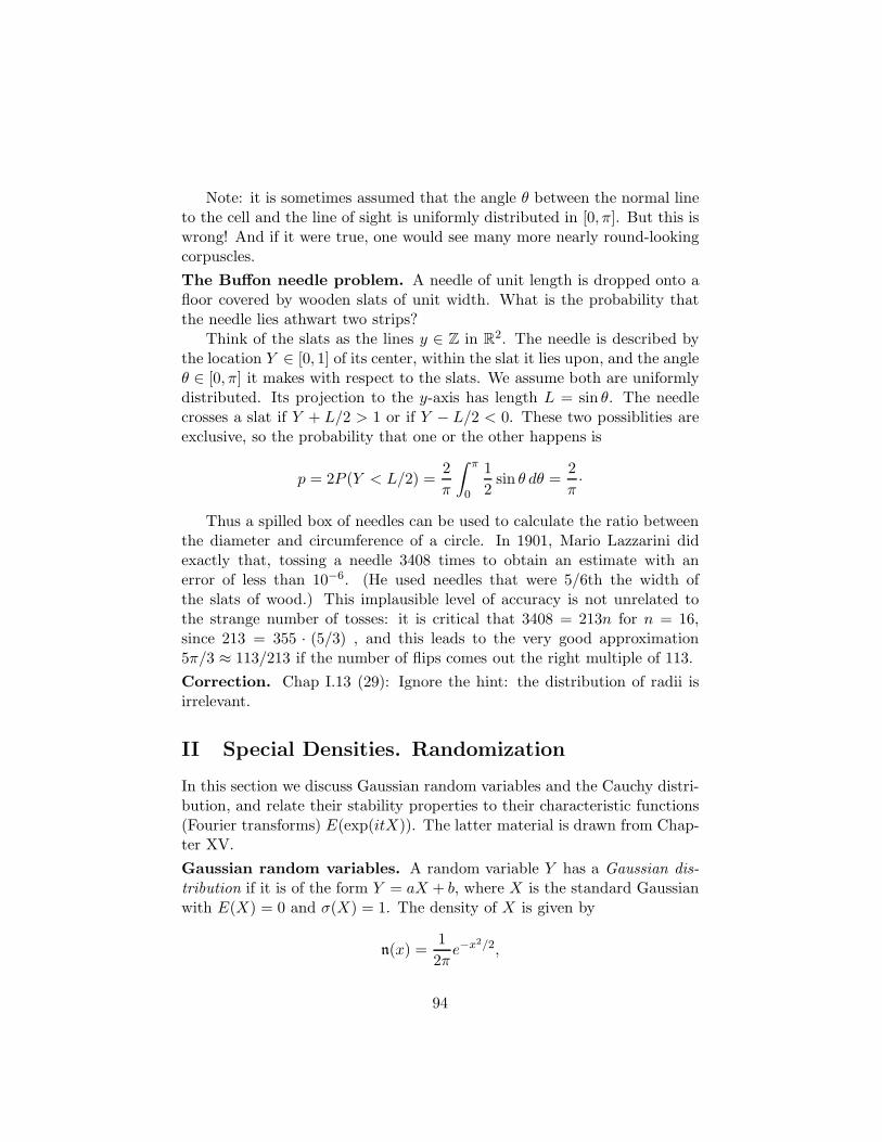
Note: it is sometimes assumed that the angle θ between the normal lineto the cell and the line of sight is uniformly distributed in [0, π]. But this iswrong! And if it were true, one would see many more nearly round-lookingcorpuscles.
The Buffon needle problem. A needle of unit length is dropped onto afloor covered by wooden slats of unit width. What is the probability thatthe needle lies athwart two strips?
Think of the slats as the lines y ∈ Z in R2. The needle is described by
the location Y ∈ [0, 1] of its center, within the slat it lies upon, and the angleθ ∈ [0, π] it makes with respect to the slats. We assume both are uniformlydistributed. Its projection to the y-axis has length L = sin θ. The needlecrosses a slat if Y + L/2 > 1 or if Y − L/2 < 0. These two possiblities areexclusive, so the probability that one or the other happens is
p = 2P (Y < L/2) =2
π
∫ π
0
1
2sin θ dθ =
2
π·
Thus a spilled box of needles can be used to calculate the ratio betweenthe diameter and circumference of a circle. In 1901, Mario Lazzarini didexactly that, tossing a needle 3408 times to obtain an estimate with anerror of less than 10−6. (He used needles that were 5/6th the width ofthe slats of wood.) This implausible level of accuracy is not unrelated tothe strange number of tosses: it is critical that 3408 = 213n for n = 16,since 213 = 355 · (5/3) , and this leads to the very good approximation5π/3 ≈ 113/213 if the number of flips comes out the right multiple of 113.
Correction. Chap I.13 (29): Ignore the hint: the distribution of radii isirrelevant.
II Special Densities. Randomization
In this section we discuss Gaussian random variables and the Cauchy distri-bution, and relate their stability properties to their characteristic functions(Fourier transforms) E(exp(itX)). The latter material is drawn from Chap-ter XV.
Gaussian random variables. A random variable Y has a Gaussian dis-tribution if it is of the form Y = aX + b, where X is the standard Gaussianwith E(X) = 0 and σ(X) = 1. The density of X is given by
n(x) =1
2πe−x2/2,
94
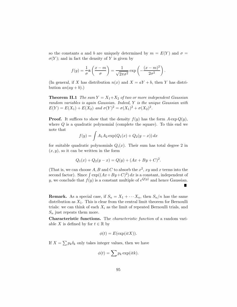
so the constants a and b are uniquely determined by m = E(Y ) and σ =σ(Y ); and in fact the density of Y is given by
f(y) =1
σn
(x − m
σ
)=
1√2πσ2
exp
(−(x − m)2
2σ2
).
(In general, if X has distribution n(x) and X = aY + b, then Y has distri-bution an(ay + b).)
Theorem II.1 The sum Y = X1+X2 of two or more independent Gaussianrandom variables is again Gaussian. Indeed, Y is the unique Gaussian withE(Y ) = E(X1) + E(X2) and σ(Y )2 = σ(X1)
2 + σ(X2)2.
Proof. It suffices to show that the density f(y) has the form A exp Q(y),where Q is a quadratic polynomial (complete the square). To this end wenote that
f(y) =
∫A1A2 exp(Q1(x) + Q2(y − x)) dx
for suitable quadratic polynomials Qi(x). Their sum has total degree 2 in(x, y), so it can be written in the form
Q1(x) + Q2(y − x) = Q(y) + (Ax + By + C)2.
(That is, we can choose A,B and C to absorb the x2, xy and x terms into thesecond factor). Since
∫exp((Ax+By+C)2) dx is a constant, independent of
y, we conclude that f(y) is a constant multiple of eQ(y) and hence Gaussian.
Remark. As a special case, if Sn = X1 + · · ·Xn, then Sn/n has the samedistribution as X1. This is clear from the central limit theorem for Bernoullitrials: we can think of each Xi as the limit of repeated Bernoulli trials, andSn just repeats them more.
Characteristic functions. The characteristic function of a random vari-able X is defined by for t ∈ R by
φ(t) = E(exp(itX)).
If X =∑
pkδk only takes integer values, then we have
φ(t) =∑
pk exp(itk).
95
Thus φ is obtained from the generating function∑
pksk by substituting
s = exp(it); it records the values of the generating function on the unitcircle in the complex plane. In this case φ(t + 2π) = φ(t).
On the other hand, if X has density f(x), then
φ(t) =
∫ ∞
−∞eitxf(x) dx.
Thus φ(t) is essentially the Fourier transform of the function f(x).Let us note some formal properties of the characteristic function.
1. We have φ(0) = 1 and |φ(t)| ≤ 1.
2. If Y = aX + b, then φY (t) = exp(itb)φX (at).
3. We have φ′(0) = E(iX), φ′′(0) = −E(X2), and φ(n)(0) = inE(Xn),assuming the moments E(Xn) exist.
Another critical property is:
Theorem II.2 If X and Y have the same characteristic function, then theyhave the same distribution.
But the most crucial connection with probability theory comes from:
Theorem II.3 The characteristic function of a sum X = X1 + X2 of twoindependent random variables is given by φ(t) = φ1(t)φ2(t).
Proof. We have E(exp(it(X1 + X2))) = E(exp(itX1))E(exp(itX2)).
We can now revisit the stability properties of the Gaussian.
Theorem II.4 The characteristic function of a Gaussian random variableX is another Gaussian, of the form
φ(t) = exp(ibt) exp(−a2t2/2). (II.1)
We have b = 0 if E(X) = 0.
Proof. By the properties above, it suffices to treat the case of the standardGaussian with E(X) = 0 and E(X2) = 1. Then by completing the square,we have
φ(t) =1√2π
∫exp(−(x2 − 2it)/2) dx
=1√2π
∫exp(−(x − it)2/2) exp(−t2/2) dx = exp(−t2/2).
96
Since the product of two Gaussian function as in (II.1) is again of thesame form, we find:
Corollary II.5 The sum Y = X1+· · ·Xn of two or more Gaussian randomvariables has a Gaussian distribution.
The exact distribution is determined by E(Y ) =∑
E(Xi) and Var(Y ) =∑Var(Xi).
Law of large numbers. Let Sn = X1 + · · ·Xn be a sum of independentrandom variables all with the same characteristic function φ. Then the char-acteristic function of Sn is given by φn(t) = φ(t)n. Hence the characteristicfunction of Sn/n is given by
µn(t) = φ(t/n)n.
For example, if X1 is Gaussian then µn(t) = exp(−t2/2n) → 1 as n → ∞.This is a reflection of the fact that Sn/n → 0, and it holds more generally ifE(X) = 0 and E(X2) is finite.
Cauchy random variables. Recall that the standard Cauchy randomvariable X with density f(x) = 1/(π(1 + x2)) has E(|X|) = ∞. Let us seehow this behavior is reflected in its characteristic function.
Theorem II.6 The characteristic function of the standard Cauchy randomvariable is given by
φ(t) = exp(−|t|).
Proof. This computation is best done by complex analysis; for t > 0, thefunction exp(itz) is rapidly decreasing as Im z → ∞, and 1 + z2 vanishes atz = i; thus by the residue theorem, we have
φ(t) =1
π
∫
R
exp(itz dz)
1 + z2=
2πi
πResz=i
exp(itz)
1 + z2= 2i
exp(−t)
2i= exp(−t).
For t < 0 we get φ(t) = exp(+t).
Note that φ′(0) does not exist. However the right and left handed deriva-tives exist and sum to zero. This reflects the fact that the Cauchy principalvalue of the expectation is zero, i.e. limN→∞
∫ N−N x dx/(1 + x2) = 0.
Failure of averaging. What happens if we take repeated Cauchy obser-vations and average them?
97
Theorem II.7 The average Sn/n = (X1 + · · · + Xn) of a sequence of in-dependent, identically distributed Cauchy random variables has the samedistribution as each one.
Proof. We have µn(t) = φ(t/n)n = exp(−|t|/n)n = exp(−|t|).
This gives a useful stability property, as well as a strong example offailure of averaging to converge.
The central limit theorem. We can now indicate a conceptually simpleproof of the central theorem, although some technical details need to beverified to make it fully rigorous.
Suppose X1, . . . ,Xn are independent random variables with a commondistribution, and E(Xi) = 0 and E(X2
i ) = 1. Let φ(t) be the correspondingcharacteristic function, and let φn(t) be the characteristic function of
S∗n =
X1 + · · ·Xn√n
·
We then haveφn(t) = φ(t/
√n)n.
Now our assumptions on mean and variance imply
φ(t) = 1 − t2/2 + o(t2).
Thus
φn(t) ∼(
1 − t2
2n
)n
→ exp(−t2/2)
as n → ∞, and the right hand side is the characteristic function of thestandard Gaussian. This shows that S∗
n converges to the standard Gaussiandistribution, at least on the level of characteristic functions.
98