Probability Review Lecture Notes

Lectures 1-4

These notes summarize the ideas and provide examples. A change in font color

(usually to the red “Comic Sans” font illustrated in this footnote) indicates

exercise solutions that the reader is encouraged to work through. In some cases,

these solutions are in text boxes.

Occasional references are made to the following textbook: Bruce Bowerman, Richard O’Connell, Emily Murphree, & J.B. Orris (2015), Essentials of

Business Statistics, 5th Edition, McGraw-Hill/Irwin.

© 2018, Bruce Cooil

This material is made available for the personal, noncommercial educational and scholarly use of

the students of Mgt. 6381 and Mgt. 7782 at the Owen Graduate School of Management. It may

not be used for any other purpose, or distributed or made available to others without permission.

Page 1 of 46

Probability Review Lecture Notes

Pages

Lecture 1:

Probability Theory

3

Events, Sample Space 3Unions & Intersections 4Trees 6Conditional Probability 7Multiplication Rule 7Independence 7More Examples 8 Sensitivity &Specificity 9

Lecture 2:

Random Variables (RVs)

& Distributions

10

Definitions, Notation, & Ideas 10Probability Distribution 11Expected Value (Mean) 12Variance & Standard

Deviation 12Means and Variances of

Linear Functions 13

Summary & Addendum to Lectures 1-2

15

Pages

Lecture 3:

Binomial Distribution

18

Bernoulli Distribution: Mean

and Variance 18

Binomial Mean, Variance

and Probabilities 19

Combinations and Trees 20More Examples 22Binomial Tables 23

Lecture 4:

Normal Distribution

26

The Normal Table 27

Finding Probabilities for

Standard Normal RVs 29

Finding Probabilities for

General Normal RVs 30

Expectations and Variances

of Sums of RVs Variables 31

Looking Beyond Lectures 1-4:

Central Limit Theorem

32

Examples 1-4: Four

Simulations 35

See the Bottom Right Corner of Each Page for the Document Page Numbers Listed Here.

(If you download this document as a PDF file and use these page links, “ALT <−” will bring you back to this page.)

Page 2 of 46

Lecture 1: Probability Concepts and Notation

Reference: Bowerman, O’Connell, Orris & Murphree (5th Ed).Ch. 4: 4.1-4.5, especially: 4.3-4.5.

Outline:A. Definitions and Ideas

1. Sample Space, Events and Complements2. Probability of Intersection3. Probability of Union

B. Conditional Probability1. Definition2. Multiplication Rule3. TREES4. Independence (vs. Mutually Exclusive Events)

Imagine an industry where there have been 200 new products in the last few

years. We categorize them two ways: according to how successful they

eventually were, and according to whether or not a preliminary evaluation

indicated success. Define the outcomes or events as follows:

G = event that my preliminary evaluation is "good"; S = event that product is huge success;M = event that product is medium success (will not be continued); F = event that product is a failure

(specific examples: software or hardware products, books, movies).

S M F TOTAL

G 60 60 30 150

GG 10 20 20 50

TOTAL 70 80 50 200

These 200 products are a “sample space.” “Sample space” refers to all

possible outcomes of a statistical experiment. Here, the statistical

experiment is the choice of one product.

Events

Any subset of the sample space is an event: S, M, F, G, and GG are all events.

Each occurs with a certain probability, e.g., P[G] = 150/200 = 0.75.GG is the complement of G ,i.e., the event G does not occur,

P[GG ] = 1 - P[G] = .25 (or 50/200).

Page 3 of 46

Intersections

The intersection of two events refers to the event where they both occur. For

example,“G1S” refers to the event that the preliminary evaluation is good

and the product went on to be a huge success: note that both G and S occur

for 60 products, so

P[G 1 S] / P[“G and S”]=60/200 = 0.30.

Similarly,

P[G- 1 M] = 20/200 = 0.1;

P[S 1 F] = 0/200 = 0.

Unions

The union of two events refers to the event of either or both occurring. So

for example,

P[GcS] / P[“G or S”]= 160/200 = 0.80,

P[McGG ] = 110/200 = 0.55.

One can use Poincaré's formula (also known as the “Addition Rule,” p.166)

to calculate the probability of a union:

P(ScG) = P(S) + P(G) - P(S1G) = 70/200 + 150/200 - 60/200

(because 60/200 is included in each of the first two probs.)

= 160/200 = 0.80.

Also for mutually exclusive events

P[ScM] = P[S] + P[M]

because S and M are mutually exclusive so that P[S1M]=0. Note:

P[McG] = (80 + 150 -60)/200 = 0.85 or 85%;

P[Fc M] = (50 + 80)/200= 0.65 or 65% .

General Comments

McF is the same as FcM. M1F is the same as F1M (this is the “null”

or empty set, sometimes written `).

Page 4 of 46

S M F TOTAL

G 60 60 30 150 𝐏𝐏[ 𝐆𝐆� ⋂𝐌𝐌] = 𝟐𝟐𝟐𝟐/𝟐𝟐𝟐𝟐𝟐𝟐

𝐆𝐆� 10 20 20 50

TOTAL 70 80 50 200

S M F TOTAL

G 60 60 30 150 𝐏𝐏 [𝐒𝐒⋂𝐅𝐅] = 𝟐𝟐/𝟐𝟐𝟐𝟐𝟐𝟐

𝐆𝐆� 10 20 20 50

TOTAL 70 80 50 200

S M F TOTAL

G 60 60 30 150 𝐏𝐏 [𝐌𝐌 ⋃𝐆𝐆] = (𝟖𝟖𝟐𝟐+ 𝟏𝟏𝟏𝟏𝟐𝟐− 𝟔𝟔𝟐𝟐)/𝟐𝟐𝟐𝟐𝟐𝟐

𝐆𝐆� 10 20 20 50

TOTAL 70 80 50 200

S M F TOTAL

G 60 60 30 150 𝐏𝐏 [𝐅𝐅 ⋃𝐌𝐌] = (𝟏𝟏𝟐𝟐+ 𝟖𝟖𝟐𝟐)/𝟐𝟐𝟐𝟐𝟐𝟐

𝐆𝐆� 10 20 20 50

TOTAL 70 80 50 200

Page 5 of 46

Probabilities Corresponding to Table on Page 3

S M F TOTAL

G .3 .3 .15 .75

GG .05 .1 .1 .25

TOTAL .35 .4 .25 1

(I've simply divided all of numbers in the original table by the sample size of 200.)

The Same Information Organized in a Tree

Step 1 Step 2 OUTCOME PROBABILITY

S (60/150=.4) G 1 S .3

G(.75) M (.4) G 1 M .3

F (.2) G 1 F .15

S ( .05/.25=0.2 ) GG 1 S .25(.2)= .05

GG( .25 ) M ( .1/.25 = 0.4 ) GG 1 M .25(0.4)= .1

F ( 0.4 ) GG 1 F .25(0.4)= .1Conditional Probability

The parenthetical probabilities next to S, M, and F in the diagram above are

conditional probabilities. The conditional probability of S given G is written as

“P[S|G]” and defined as: P[S|G] = P[S1G]/P[G].

Thus,

P[S|G] = .3/.75 = 0.4.

Note that this is different from P[G|S], since

P[G|S] = P[G1S]/P[S] = .3/.35 = 0.857.

Page 6 of 46

Multiplication Rule

The multiplication rule allows us to find the probability of an intersection from a

conditional probability and the unconditional probability of the event on which we are

conditioning. The rule is simply a consequence of the definition of conditional

probability. This rule is used to derive the event probabilities in the last column of a

probability tree. In general for any two events A and B:

P[A1B]= P[A|B] P[B]. (Also: P[A1B] = P[B|A] P[A].)

This works because we're recovering the numerator of the conditional probability by

multiplying by its denominator!

Independence

Note that the probability of M is the same whether or not G occurs since,

P[M|G] = 0.4 , and P[M] = 0.4.

When this happens, we say that M and G are independent. If

M and G are independent, it’s also true that P[G|M] = P[G] (=.75). In general, two events

A and B are independent if

P[B|A] = P[B] (or if P[A|B]=P[A]).

An equivalent definition: independence of A and B means

P(A1B)=P(A)P(B).

Main IdeasNotation: definitions of A1B=B1A, AUB=BUA (these operations are commutative!)

Rule of Unions (Poincare's formula): P(AUB) = P(A) + P(B) - P(A1B)

Definition of Conditional Probability: (P(A#B) / [P(A1B)/P(B)]

Multiplication Rule: P(A1B) = P(A#B) P(B)

Independence: A & B are independent if P(A1B) = P(A)P(B)Or, equivalently, if P(A|B) = P(A)Or, equivalently, if P(B|A) = P(B)

Page 7 of 46

More Examples (Lecture 1)

1. A manufacturing process falls out of calibration 10% of the time. When it iscalibrated, defective nails are produced with a probability of 1%. When it is notcalibrated, the probability of producing a defect is 0.1.

Let C=event process is calibrated; D=event of producing defect.Outcome Probability

D(.01) C 1 D .009C (0.9)

D_(0.99) C 1 D

_.891

D(.1) C_ 1 D 0.01

C_(0.1)

D_(0.90) C

_ 1 D

_0.09

a. What is the overall probability of getting a defective?

P(D) = P (C 1 D) + P(C_ 1 D) = 0.009 + 0.01 (Using Tree above) = .019

b. What is the probability that I will sample a defective and the process is outof calibration (i.e., what is the probability of the intersection of these twoevents)?P(C_ 1 D) = 0.01 (based on tree above)

c. I randomly select 1 nail that has just been produced. It's defective! What'sthe probability the process needs calibration?P(C_|D) = P(C

_ 1 D) /P(D) = 0.01/0.019 = 0.526

2. I have two career opportunities. Opportunity A will occur with probability0.4. Opportunity B will occur with probability 0.3. Assume theopportunities are independent.

a. What is the probability I will have both opportunities?

P( A 1 B) = P(A) * P(B) = 0.4(0.3) = 0.12

b. What is the probability that I will have at least 1 opportunity?

P( A c B) = P(A) + P(B) - P(A 1 B) = 0.4+0.3-0.12 = 0.58

Page 8 of 46

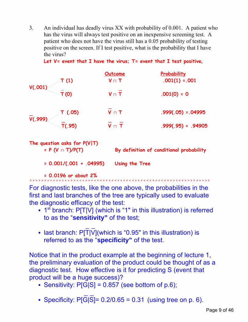
3. An individual has deadly virus XX with probability of 0.001. A patient whohas the virus will always test positive on an inexpensive screening test. Apatient who does not have the virus still has a 0.05 probability of testingpositive on the screen. If I test positive, what is the probability that I havethe virus?Let V= event that I have the virus; T= event that I test positive.

Outcome Probability T (1) V 1 T .001(1) =.001

V(.001) T_

(0) V 1 T_

.001(0) = 0

T (.05) V_ 1 T .999(.05) =.04995

V_(.999)

T_(.95) V

_ 1 T

_.999(.95) = .94905

The question asks for P(V|T) = P (V 1 T)/P(T) By definition of conditional probability

= 0.001/(.001 + .04995) Using the Tree

= 0.0196 or about 2%**************************************************************

For diagnostic tests, like the one above, the probabilities in thefirst and last branches of the tree are typically used to evaluatethe diagnostic efficacy of the test: C 1st branch: P[T|V] (which is “1" in this illustration) is referred

to as the “sensitivity” of the test;

C last branch: P[T_|V_](which is “0.95" in this illustration) is

referred to as the “specificity” of the test.

Notice that in the product example at the beginning of lecture 1,the preliminary evaluation of the product could be thought of as adiagnostic test. How effective is it for predicting S (event thatproduct will be a huge success)? C Sensitivity: P[G|S] = 0.857 (see bottom of p.6);

C Specificity: P[G_|S_]= 0.2/0.65 = 0.31 (using tree on p. 6).

Page 9 of 46

Lecture 2: Random Variables and Probability Distributions

Reference: Ch. 5: 5.1-5.2, App. 5.3; Outline

C Random Variable(RV): What Is It and Why Use It?C Probability Distributions of RVC Expected Value (or Mean) of RVC Variance (and Standard Deviation) of RVC Mean and Variance of Linear Function of RV

(If Y = a + bX, then μY = a + bμX and σY = bσX)

Random Variables

A random variable (rv) is simply a way of representing numerical outcomes thatoccur with different probabilities. A discrete rv can assume only a countablenumber of values. A continuous rv assumes an uncountably infinite number ofvalues corresponding to the points on an interval (or more than one interval).

EXAMPLE:I'm a consultant whose income depends on the number of projects that I finish. Let Xrepresent the number of projects that I complete in a month:

X=# of projects completed in month.

X is an example of a discrete rv. Assume that I undertake 2 new projects in a month,there is a probability of 0.6 that I will complete each one, and the projects areindependent.

A probability tree provides one way to analyze this situation. Finish this one!

Let S successful completion of project i.i

Step 1 Step 2(1st Project) (2nd Project) Outcomes Probability

(.6) 2 successes .36S2

(.6)S1

(.4) success, failure .24S2

(.6) failure, success .24S2

(.4) S1

(.4) 2 failures .16S2

Page 10 of 46

Lecture 2 Pg. 2

The PROBABILITY DISTRIBUTION of X can be summarized with the function P(x).

x P(x) xP(x) (x-μ)2 (x-μ)2P(x) x2P(x)

0 0.16 0 (0-1.2)2 1.44(0.16) 0

=1.44

1 0.48 0.48 (1-1.2)2 0.04(0.48) 0.48

=0.04

2 0.36 0.72 (2-1.2)2 0.64(0.36) 1.44

=0.64

TOTAL: 1.2 0.48 1.92

This is the variance of X;common notation: “ . ”2

XFX = (0.48)

½ = 0.69

This is the mean of X; common notation:

“μX” Or “E(X)”

This is the mean of therandom variable X2 or“E(X2).”

Page 11 of 46

Lecture 2 Pg. 3

Expected Value (Or Mean) of X: μ / E(X) / 3 xP(x)

The expected value of a random variable is simply the weighted average of its

possible values, where each value is weighted by its probability.

In English it is often referred to as: "the population mean (or average)," "the

distribution mean," or "the expected value."

Variance of X: σ2 / E[(X-μ)2] / 3 (x-μ)2P(x)

The variance may also be calculated as σ2 = 3 x2P(x) - μ2.

Note the first term in this last expression is just the expectation or average value of

X2.

Because the variance is in squared units, people often use its square root σ, the

standard deviation, as an alternative measure of how "spread-out" the distribution is.

Standard Deviation of X: σ = [Variance of X]½

Another Example:

Suppose Y is my total income in thousands per month:

Y = 5 + 10X

where X is the number of projects completed. Use E(X) (μX), and Var(X) (σ2

X) to

find: E(Y), Var(Y) and σ Y .

μ Y = 5 + 10 μ X = 5+(10*1.2)= 17 thousand dollars

σ2 Y = 102 σ2

X = 100(0.48) =48 (thousand dollars)2

σ Y = 10 σ X = 10 (0.69) = 6.9 thousand dollarsPage 12 of 46

Lecture 2 Pg. 4

Suppose

Y = a + bX,

where "a" and "b" are just constants (not random variables). We can find the mean of

Y as the same linear function of the mean of X,

[Mean of Y] = a + b[Mean of X].

What about the variance? The variance of Y is

[Variance of Y] = b2[Variance of X],

and if we take square roots of both sides of last equation:

[Standard Deviation of Y] = b[Standard Deviation of X].

Example:

The distribution of the number of UHD TVs sold at an electronics store is shown below.

UHD TVs Sold Per Week

Prob

abili

ty

543210

0.5

0.4

0.3

0.2

0.1

0.0

Probability Distribution of UHD TVs Sold Per Week

Find the mean and standard deviation of this distribution.

E(X) = 0(.03) + 1(0.2) + 2(.5) + 3(.2) + 4(.05) + 5(.02) = 2.1;

Var(X) = (0-2.1)2(.03) + (1-2.1)2(.2) + (2-2.1)2(.5) + (3-2.1)2(.2)

+ (4-2.1)2(.05) + (5-2.1)2(.02) = 0.89 ==> σX = 0.94.

X= UHD TVsSold Per Week

Probability

0 0.03

1 0.2

2 0.5

3 0.2

4 0.05

5 0.02

Page 13 of 46

Lecture 2 Pg. 5

Consider the distribution of Y = 5 + 2X.

Y = 5 + 2X

Prob

abili

ty

151311975

0.5

0.4

0.3

0.2

0.1

0.0

Scatterplot of Probability vs C3

Note that we can simply find the mean and standard of Y directly, using the mean

and standard deviation of X:

E(Y) = 5 + 2*E(X) = 5 + 2(2.1) = 9.2 ;

σY = 2* σX = 2(0.94) = 1.9 .

Another Example

Find the mean, variance and standard deviation of the rv

X = profit on 10 thousand dollar investment (after 1 year) in thousands of dollars.

Possible Values of X: -10 0 20

Probability: 0.3 0.4 0.3

E(X) = -10(0.3) + 0(0.4) + 20(0.3) = 3 thousand dollars;

Var(X) = E(X2)-(E(X))2 = [100(0.3) + 0(0.4) +400(0.3)] -9 =141 .

Thus: σX = %141 = 11.87 thousand dollars.Also find the mean and standard deviation of the broker’s income, I, where I (in

thousands of dollars) is defined as: I = 3 + 0.1 X.

E(I) = 3 + 0.1(3) = 3.3 thousand dollars ;

σI = 0.1(σX) = 0.1(11.87)= 1.187 thousand dollars.

X Y Probability

0 5 0.03

1 7 0.2

2 9 0.5

3 11 0.2

4 13 0.05

5 15 0.02

Page 14 of 46

Summary & Addendum to Lectures 1 & 2

Big Picture So Far

Elements of Probability Theory: Lecture 1

Definitions & Notation A Central Idea: Conditional Probability

(It’s an important concept by itself, but it also provides a way of explaining independence)

Probability Trees

Provide a way of summarizing (and reviewing) all of the major ideas and notation

Great way of solving problems that require the calculation of a conditional probability

Lecture 2

Definitions of RVs Probability Distributions Means and Variances

Page 15 of 46

At the End of Lecture 2 We Looked at Applications Where It’s Useful to Remember That: If Y = a + bX Then: ●E(Y) = a + bE(X) (OR: XY ba µ+=µ ) ● XY bσ=σ Remembering this can save a lot of labor. What Happens With Sums Of RVs? • The Mean (Or Expectation) Of A Sum

Of RVs Is The Sum Of The Means Of Those RVs

• If The RVs Are Independent, Then The

Variance Of A Sum Of RVs Is The Sum Of The Variances Of Those RVs

Page 16 of 46

Example: Define independent RVs:

N1 = profit from investment 1 N2= profit from invesment 2 T= total profit = N1 + N2

Assume: E(N1) = 2, E(N2) = 3 (millions $) 5.12

1 =σN , 5.222 =σN

Find the Expectation and Standard Deviation of Total Profit:

E(T) = 2 + 3 = 5 million

Var(T) = 1.5 + 2.5, So σ = (4)1/2 = 2

(This Idea Applies to Any Type of RV, So That Any Specific Application Understates Its Importance.)

Imagine How Much Work This Would Be If I Had to Go Back and Calculate the Mean and Variance Directly from the Distribution of T!

Page 17 of 46

Lecture 3: The Binomial Distribution

Reference: Ch. 4: 4.6; Ch. 5: 5.3Outline:

! Bernoulli Distribution μ = p, σ2 = p(1-p)! Binomial Distribution μ = np, σ2 = np(1-p)

We Consider Means, Variances and Calculating Probabilities (Directly or withTables)

Bernoulli Distribution

Examples:

(1) X = # of times I get a “6" on one roll of a die.

P[X=1] = P[getting a “6" on a roll of a die] = 1/6

P[X=0] = 5/6.

E[X] = 0(5/6) + 1(1/6) = 1/6.

Var(X) = E(X2)- μ2 = 'x2P(x) - μ2 =[02(5/6) + 12(1/6)] -(1/6)2

= 1/6-(1/6)2 OR 1/6(1-1/6).

(2) 20% of all customers prefer brand A to brand B. I

interview just 1 customer. Consider the distribution of rv X, where: X = #

(of 1) who prefer A to B.

P[X=1] = 0.2 , P[X=0]= 0.8 , E(X) = 0.2.

Var(X)= 0.2(0.8) = 0.16.

Examples Above Are Illustrations of Bernoulli Random Variables

A Bernoulli random variable is simply a variable, X, that indicates whether or not

something happens. In general, X might be thought of as

X = # of successes in 1 trial (or attempt).

Suppose success occurs with probability p , then:

P[X=1]= “prob. of 1 success” = p; P[X=0] = 1-p

AND: E(X)= p (the prob. of success),

Var(X) = p - p2 = p(1-p) = [prob. of success]*[prob. of failure].

Bottom Line: The mean of a Bernoulli random variable is the probability of

success; its variance is the product of the probability of success and the

probability of failure.

Page 18 of 46

Binomial Distribution

Examples of Binomial Random Variables (rvs):

(1) Y = Number of times "6" comes up in 3 rolls of die.

Possible Values: 0, 1, 2, 3.

(2) Suppose there are in 4 independent business deals, & each will result in a profit

with probability of 0.7. Consider the distribution of

Y = # of profitable deals (of 4).

Possible Values: 0, 1, 2, 3, 4.

(3) Assume 20% of all customers (an infinite population) prefer brand A to brand B.

Only 10 customers are interviewed.

Consider the distribution of

Y = # of customers of 10 who prefer brand A to brand B.

Possible Values: 0, 1, 2, 3, 4, ..., 10.

A General Binomial Random Variable

As illustrated above, many applications require that we work with a rv that represents a

slight generalization the Bernoulli rv,

Y = # of successes in n trials,

where the trials are assumed to be independent & each results in a success with the same

probability p. Y is referred to as a binomial rv (& the sequence of trials is sometimes

referred to as a Bernoulli process).

Note that a binomial rv is really just the sum of n Bernoulli rvs (where n = number of

trials). Consequently, the mean and variance of Y are just n times the mean and variance

of the corresponding Bernoulli rv: E[Y] = n C p ; Var[Y] = n C p(1-p)

(because “p” and “p(1-p)” are the Bernoullli mean and variance).

Probabilities can be found in Table A.1, App. A (pp. 599-603) or probabilities can be

calculated directly using the following formula:

P[Y=y] = “prob. of y successes in n trials”

= [# of sequences of n trials that have exactly y successes]

* [probability of each such sequence]

= = (also written “ ”).yny pp

yny

n

)()!(!

!1

n

yp py n y

( )1

Page 19 of 46

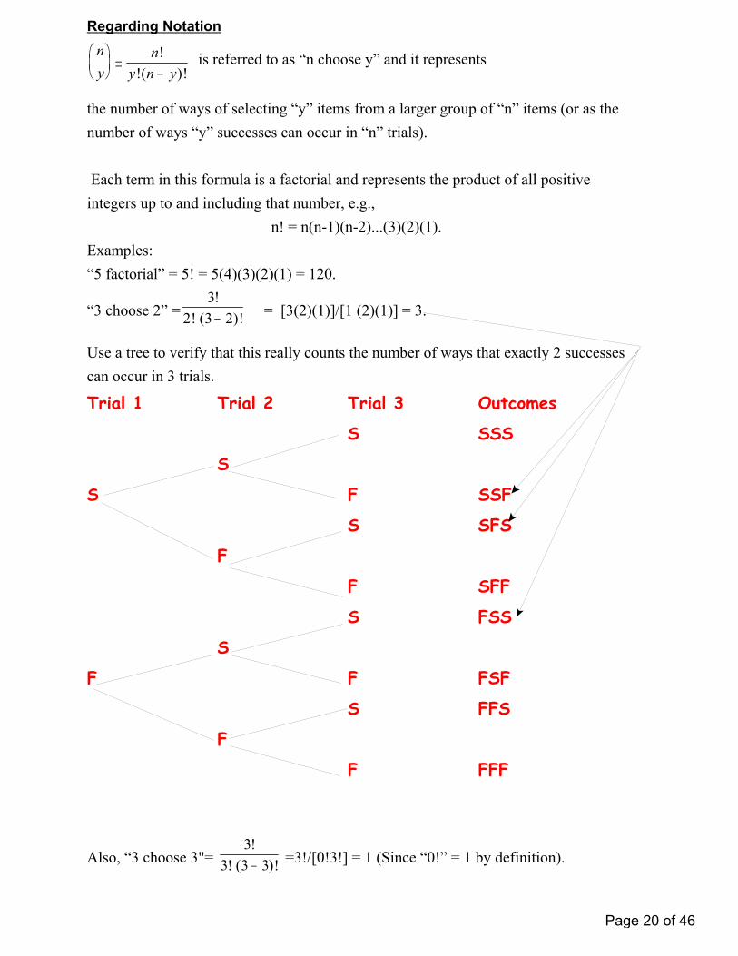
Regarding Notation

is referred to as “n choose y” and it represents n

yn

y n y

!

!( )!

the number of ways of selecting “y” items from a larger group of “n” items (or as the

number of ways “y” successes can occur in “n” trials).

Each term in this formula is a factorial and represents the product of all positive

integers up to and including that number, e.g.,

n! = n(n-1)(n-2)...(3)(2)(1).

Examples:

“5 factorial” = 5! = 5(4)(3)(2)(1) = 120.

“3 choose 2” = = [3(2)(1)]/[1 (2)(1)] = 3.3

2 3 2

!

! ( )!

Use a tree to verify that this really counts the number of ways that exactly 2 successes

can occur in 3 trials.

Trial 1 Trial 2 Trial 3 Outcomes

S SSS

S

S F SSF

S SFS

F

F SFF

S FSS

S

F F FSF

S FFS

F

F FFF

Also, “3 choose 3"= =3!/[0!3!] = 1 (Since “0!” = 1 by definition). 3

3 3 3

!

! ( )!

Page 20 of 46

“4 choose 2"= = 4!/[2!2!] = 6.4

2 4 2

!

! ( )!

Use a tree to verify this is number of ways that exactly

2 successes can occur in 4 trials.

Trial 1 Trial 2 Trail 3 Trial 4 Outcomes

S SSSS

S

F SSSF

S S SSFS

F

F SSFF

S S SFSS

S

F F SFSF

S SFFS

F

F SFFF

S FSSSS

F FSSF

S S FSFS

F

F FSFF

F S FFSS

S

F F FFSF

S FFFS

F

F FFFF

Number of ways of having exactly 2successes in 4 trials

Page 21 of 46

Sometimes the trees are much too complicated. For example, suppose I want to count the

number of ways 3 successes can occur in 10 trials. By far the easiest way is to

mechanically use the formula:

“10 choose 3"= = .)!310(!3

!10

120

!3

8*9*10

!7!3

!7*8*9*10

Notice that in general: “n choose y” is the same as “n choose (n-y).” For example,

“10 choose 3" is equal to “10 choose 7." Arithmetically, this is obviously true, but logically it also must be true: when I choose 3 from 10, I am simultaneously not choosing the other 7, so the number of subsets of size 3 must be equal to the number of subsets of size 7.

Applications to the Binomial Example 2 on Page 19:

Example 2: Write down the probability distribution of

Y = # of profitable deals (of 4), p = 0.7 .This has a Binomial distribution (n=4, p=0.7).

E(Y)= 4(0.7) = 2.8 ;Var(Y) = 4(0.7)(0.3) = 0.84; σY= (0.84)

½ = 0.92.Probability of exactly 2 profitable deals:

P[Y = 2] = (Also see Table.)26460307022

4 22 .).().(!

!

Probability of at least 2 profitable deals:

P[Y > 2] = P(2)+P(3)+P(4)= 1-[P(0)+P(1)] ;

P(0)= ; 0081030307040

4 440 .).().().(!!

!

P(1)= 07560307031

4 31 .).().(!!

!

So, P[Y > 2] = 1-(0.0081+0.0756) = 0.9163 .(Or UseTable.)Probability of at most 2 profitable deals:

P[Y < 2] = P(0)+ P(1) + P(2) =0.0081 + 0.0756 + 0.2646 =0.3483.Binomial Tables are provided on the next pages. These are in Bowerman, et al., but are originally from

Hildebrand, D. & Ott, L.(1991) Statistical Thinking for Managers, Boston: PWS-Kent.

Page 22 of 46

Page 23 of 46

Page 24 of 46

Last Example!

Define r.v. W as:

W = # of business failures (of 8 new ventures).

W is binomial with n=8, p= 0.4.

Find the following probabilities:

P[W=6] = = 0.0413.26 )6.0()4.0(

)!68(!6

!8

P[W >6] = P(7) + P(8)

= 0.0079 + 0.0007 = 0.0086.

P[ W # 6] = 1- 0.0086 = 0.9914.

What is the most probable outcome? Answer: W=3.

P[W=3] = = 0.2787.53 6040

3838 ).().(

)!(!!

Find the mean and variance of W:

E[W] = np = 8*0.4 = 3.2;

Var[W] = np(1-p)= 3.2*0.6 = 1.92.

Page 25 of 46

Lecture 4: Normal Distribution

Reference: Ch. 6: 6.1-6.3 (especially 6.3); Appendix 6.3Outline:

! Description of Normal & Standard Normal Distributions! Standardizing to Find Probabilities! Sums of Normal RVs

DescriptionThe normal distribution is a continuous, bell-shaped distribution (e.g., see the figures insection 6.3or at http://en.wikipedia.org/wiki/Normal_distribution). By standardizing anynormal rv, it is possible to calculate the probabilities with respect to a standard normaldistribution (i.e., a normal distribution with mean of 0 and standard deviation of 1). Thetables on the next two pages provides a tabulation of standard normal cumulativeprobabilities. This table is also in section 6.3 of the text, inside the back cover, and inAppendix A of the text (Table A.3).

What is the probability that a standard normal rv, Z, will lie within 1 standard deviation of

0 (its mean)?

P[-1 #Z # 1] = [Table Value at 1]- [Table value at -1]

= 0.8413 – 0.1587 = 0.6826 .Note that there is no probability content at individual points so that,

P[-1 #Z # 1] = P[-1 < Z < 1]

(i.e., whether or not we include the values at the ends of this interval, the probability

remains unchanged).

Based on the normal distribution, here are general (and somewhat dangerous) empirical

guides that are often used when people think of any symmetric and continuous

distribution:

! approximately 68% of observations fall within 1 standard deviation of the mean

! approximately 95% fall within 2 standard deviations

! nearly all fall within 3 standard deviations.

Page 26 of 46

Lecture 4 Pg. 2

Standard Normal Cumulative Probability Table 0

Cumulative probabilities for NEGATIVE z-values are shown in the following table: z .00 .01 .02 .03 .04 .05 .06 .07 .08 .09

-3.0 .0013 .0013 .0013 .0012 .0012 .0011 .0011 .0011 .0010 .0010 -2.9 .0019 .0018 .0018 .0017 .0016 .0016 .0015 .0015 .0014 .0014 -2.8 .0026 .0025 .0024 .0023 .0023 .0022 .0021 .0021 .0020 .0019 -2.7 .0035 .0034 .0033 .0032 .0031 .0030 .0029 .0028 .0027 .0026 -2.6 .0047 .0045 .0044 .0043 .0041 .0040 .0039 .0038 .0037 .0036 -2.5 .0062 .0060 .0059 .0057 .0055 .0054 .0052 .0051 .0049 .0048 -2.4 .0082 .0080 .0078 .0075 .0073 .0071 .0069 .0068 .0066 .0064 -2.3 .0107 .0104 .0102 .0099 .0096 .0094 .0091 .0089 .0087 .0084 -2.2 .0139 .0136 .0132 .0129 .0125 .0122 .0119 .0116 .0113 .0110 -2.1 .0179 .0174 .0170 .0166 .0162 .0158 .0154 .0150 .0146 .0143 -2.0 .0228 .0222 .0217 .0212 .0207 .0202 .0197 .0192 .0188 .0183 -1.9 .0287 .0281 .0274 .0268 .0262 .0256 .0250 .0244 .0239 .0233 -1.8 .0359 .0351 .0344 .0336 .0329 .0322 .0314 .0307 .0301 .0294 -1.7 .0446 .0436 .0427 .0418 .0409 .0401 .0392 .0384 .0375 .0367 -1.6 .0548 .0537 .0526 .0516 .0505 .0495 .0485 .0475 .0465 .0455 -1.5 .0668 .0655 .0643 .0630 .0618 .0606 .0594 .0582 .0571 .0559 -1.4 .0808 .0793 .0778 .0764 .0749 .0735 .0721 .0708 .0694 .0681 -1.3 .0968 .0951 .0934 .0918 .0901 .0885 .0869 .0853 .0838 .0823 -1.2 .1151 .1131 .1112 .1093 .1075 .1056 .1038 .1020 .1003 .0985 -1.1 .1357 .1335 .1314 .1292 .1271 .1251 .1230 .1210 .1190 .1170 -1.0 .1587 .1562 .1539 .1515 .1492 .1469 .1446 .1423 .1401 .1379 -0.9 .1841 .1814 .1788 .1762 .1736 .1711 .1685 .1660 .1635 .1611 -0.8 .2119 .2090 .2061 .2033 .2005 .1977 .1949 .1922 .1894 .1867 -0.7 .2420 .2389 .2358 .2327 .2296 .2266 .2236 .2206 .2177 .2148 -0.6 .2743 .2709 .2676 .2643 .2611 .2578 .2546 .2514 .2483 .2451 -0.5 .3085 .3050 .3015 .2981 .2946 .2912 .2877 .2843 .2810 .2776 -0.4 .3446 .3409 .3372 .3336 .3300 .3264 .3228 .3192 .3156 .3121 -0.3 .3821 .3783 .3745 .3707 .3669 .3632 .3594 .3557 .3520 .3483 -0.2 .4207 .4168 .4129 .4090 .4052 .4013 .3974 .3936 .3897 .3859 -0.1 .4602 .4562 .4522 .4483 .4443 .4404 .4364 .4325 .4286 .4247 0.0 .5000 .4960 .4920 .4880 .4840 .4801 .4761 .4721 .4681 .4641

Page 27 of 46

Lecture 4 Pg. 3

Cumulative probabilities for POSITIVE z-values are in the following table:

z .00 .01 .02 .03 .04 .05 .06 .07 .08 .09 0.0 .5000 .5040 .5080 .5120 .5160 .5199 .5239 .5279 .5319 .5359 0.1 .5398 .5438 .5478 .5517 .5557 .5596 .5636 .5675 .5714 .5753 0.2 .5793 .5832 .5871 .5910 .5948 .5987 .6026 .6064 .6103 .6141 0.3 .6179 .6217 .6255 .6293 .6331 .6368 .6406 .6443 .6480 .6517 0.4 .6554 .6591 .6628 .6664 .6700 .6736 .6772 .6808 .6844 .6879 0.5 .6915 .6950 .6985 .7019 .7054 .7088 .7123 .7157 .7190 .7224 0.6 .7257 .7291 .7324 .7357 .7389 .7422 .7454 .7486 .7517 .7549 0.7 .7580 .7611 .7642 .7673 .7704 .7734 .7764 .7794 .7823 .7852 0.8 .7881 .7910 .7939 .7967 .7995 .8023 .8051 .8078 .8106 .8133 0.9 .8159 .8186 .8212 .8238 .8264 .8289 .8315 .8340 .8365 .8389 1.0 .8413 .8438 .8461 .8485 .8508 .8531 .8554 .8577 .8599 .8621 1.1 .8643 .8665 .8686 .8708 .8729 .8749 .8770 .8790 .8810 .8830 1.2 .8849 .8869 .8888 .8907 .8925 .8944 .8962 .8980 .8997 .9015 1.3 .9032 .9049 .9066 .9082 .9099 .9115 .9131 .9147 .9162 .9177 1.4 .9192 .9207 .9222 .9236 .9251 .9265 .9279 .9292 .9306 .9319 1.5 .9332 .9345 .9357 .9370 .9382 .9394 .9406 .9418 .9429 .9441 1.6 .9452 .9463 .9474 .9484 .9495 .9505 .9515 .9525 .9535 .9545 1.7 .9554 .9564 .9573 .9582 .9591 .9599 .9608 .9616 .9625 .9633 1.8 .9641 .9649 .9656 .9664 .9671 .9678 .9686 .9693 .9699 .9706 1.9 .9713 .9719 .9726 .9732 .9738 .9744 .9750 .9756 .9761 .9767 2.0 .9772 .9778 .9783 .9788 .9793 .9798 .9803 .9808 .9812 .9817 2.1 .9821 .9826 .9830 .9834 .9838 .9842 .9846 .9850 .9854 .9857 2.2 .9861 .9864 .9868 .9871 .9875 .9878 .9881 .9884 .9887 .9890 2.3 .9893 .9896 .9898 .9901 .9904 .9906 .9909 .9911 .9913 .9916 2.4 .9918 .9920 .9922 .9925 .9927 .9929 .9931 .9932 .9934 .9936 2.5 .9938 .9940 .9941 .9943 .9945 .9946 .9948 .9949 .9951 .9952 2.6 .9953 .9955 .9956 .9957 .9959 .9960 .9961 .9962 .9963 .9964 2.7 .9965 .9966 .9967 .9968 .9969 .9970 .9971 .9972 .9973 .9974 2.8 .9974 .9975 .9976 .9977 .9977 .9978 .9979 .9979 .9980 .9981 2.9 .9981 .9982 .9982 .9983 .9984 .9984 .9985 .9985 .9986 .9986 3.0 .9987 .9987 .9987 .9988 .9988 .9989 .9989 .9989 .9990 .9990

From http://www2.owen.vanderbilt.edu/bruce.cooil//cumulative_standard_normal.pdf

Page 28 of 46

Lecture 4 Pg. 4

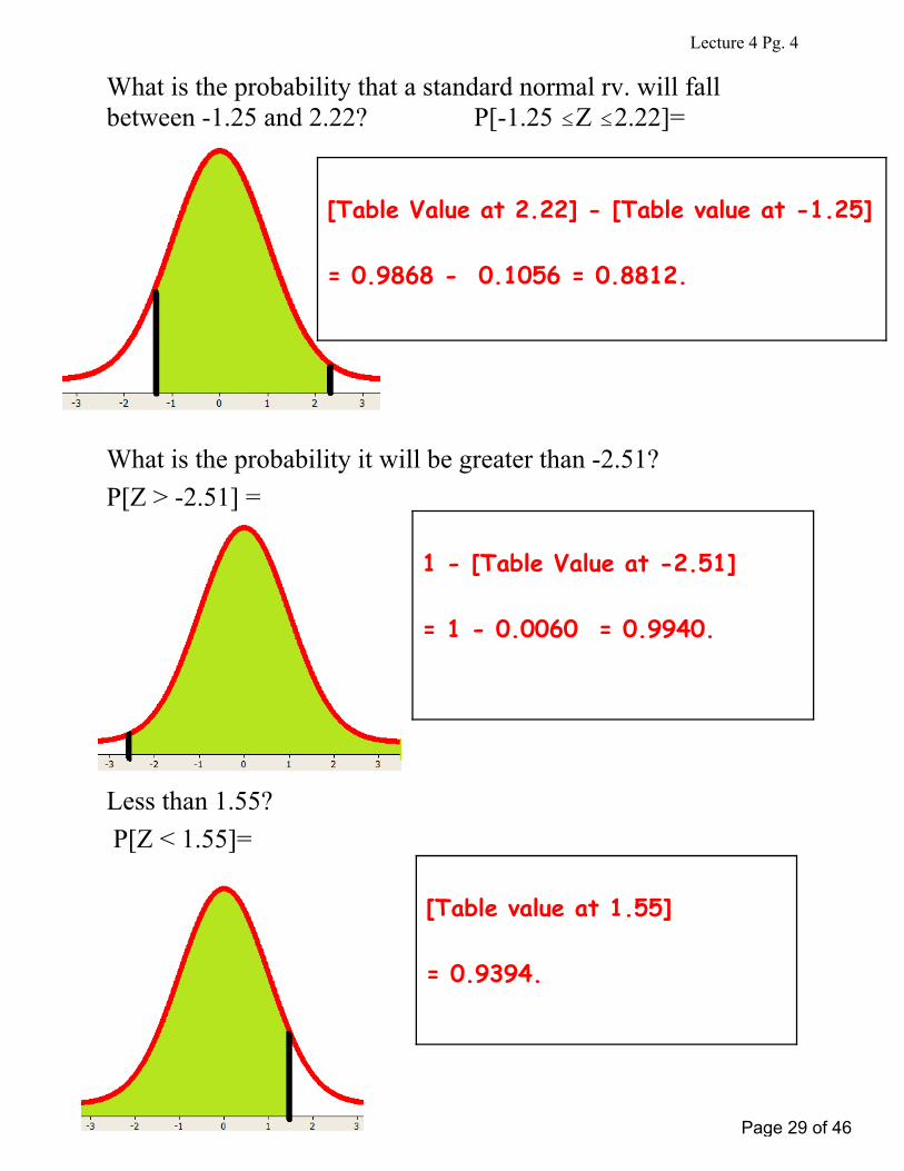
What is the probability that a standard normal rv. will fallbetween -1.25 and 2.22? P[-1.25 #Z #2.22]=

What is the probability it will be greater than -2.51?

P[Z > -2.51] =

Less than 1.55?

P[Z < 1.55]=

[Table Value at 2.22] - [Table value at -1.25]

= 0.9868 - 0.1056 = 0.8812.

1 - [Table Value at -2.51]

= 1 - 0.0060 = 0.9940.

[Table value at 1.55]

= 0.9394.

Page 29 of 46

Lecture 4 Pg. 5

EXAMPLE

Suppose X = profit (or loss) from an investment (in thousands ofdollars). Assume that we know from previous experience withthis type of investment that X is normal (μ = 5 ,σ = 2).

What is P[X > 10.5] ?

What is P[X >2.44] ?

What is the probability that I will lose money? (i.e., P[X<0]?)

What is P[3 < X < 7]?

=P[ Z > (10.5 - 5)/2 ] = P[Z > 2.75)

= 1 - [Table Value at 2.75]

= 1 - 0.9970 = 0.0030

= P[ Z > (2.44 - 5)/2 ] = P[Z > -1.28]

=1- [Table Value at -1.28] = 1 -0.1003

= 0.8997

= P[ Z < (0 - 5)/2 ] = P[Z < -2.5]

=[Table Value at -2.5] = 0.0062.

= P[ {(3-5)/2} < Z < {(7-5)/2} ]

= P[-1<Z<1]= [Table Value at 1]- [Table value at -1] = 0.8413 -0.1587 = 0.6826.

Page 30 of 46

Lecture 4 Pg. 6

Recall Two Useful Principles from Lecture 2

1) The Expectation of a Sum of RVs = Sum of the Expectations.2) If the RVs are also independent,

The Variance of the Sum of RVs = Sum of the Variances.

Normal Rvs Also Have the Following Remarkable Property

3) The RV Created By Summing Independent Normal RVs Also Has

a Normal Distribution!!!!

Application:

Assume the following RVs are in units of $1,000:

X1 = profit (or loss) from investment 1, X1 is Normal(μ = 5, σ2= 4);

X2 = profit (or loss) from investment 2, X2 is Normal(μ = 10, σ2= 5).

(Also assume these RVs are independent.)

Consider: T = total profit from both investments = X1 + X2

What is the distribution of T? (Be sure to specify its mean and variance.)

T is normal with μ = 5+10 = 15 & σ2 = 4 + 5 = 9 ( and σ = 3).

Find P[T>10].

= P[Z > (10-15)/3] = P[Z>-1.67]

= 1 - [Table Value at -1.67] = 0.9525.

Finally, what is the distribution of

I = income to a broker = 5 + 0.1X1 + 0.2X2 (in $1000)?

I has a normal distribution with

μ = 5 + (0.1)E(X1) + (0.2)E(X2) = 5+ (0.1)5 + (0.2)10 = 7.5;

σ2 = (0.1)2 Var(X1 ) + (0.2)2 Var(X2 ) = (0.1)24+ (0.2)25 = 0.24 ;

Thus: σ = (0.24)½ = 0.49. Page 31 of 46

Looking Beyond Lectures 1-4 Outline:

• The Main Reason That the Normal Distribution is SoImportant: The Central Limit Theorem (CLT)• CLT Experiments

Central Limit Theorem

Statement of CLT: Means of n independent observations from a “parent” distribution with mean μ and standard deviation σ, will have approximately a normal distribution with the same mean μ and a standard deviation of σ/√n (even if the parent distribution is very unlike the normal).

Short Statement of Theorem: Means Are Approximately Normal!

Examples: Averages of 5 customer service times (e.g., fast food restaurant) Averages of 10 product lifetimes Averages of 20 customer expenditures at retail store In each case the parent distribution of an individual observation

is positively skewed. But the histogram of 100 averages would reveal that the distribution of the averages is approximately normal.

Page 32 of 46

2

2

Illustrations: Do Your Own Experiment!The 30 averages of 4 dice thrown randomly 30 times

Stem & Leaf Display (see https://en.wikipedia.org/wiki/Stem-and-leaf_display) Units: 0.1

1 | 2 | 3 | 4 | 5 | 6 |

Results of A Previous Experiment (49 averages of 4 Dice)

Units: 0.1

1 |777 2 |277707257 3 |5220700072007552555022 4 |2207572207 5 |72220 6 |

Page 33 of 46

3

3

Discrete Parent Distribution (Outcome of One Toss of Die), and the Distributions of Means of 2, 5 & 20 Tosses

654321

300

250

200

150

100

50

0

Value of Die

Occ

urre

nces

Distribution of 1000 Tosses of a Fair Die

Graph 1

654321

300

250

200

150

100

50

0

Value of Average

Occ

urre

nces

Distribution of 1000 Averages of Two Tosses of a Fair Die

Graph 2

654321

300

250

200

150

100

50

0

Value of Average

Occ

urre

nces

Distribution of 1000 Averages of Five Tosses of a Fair Die

Graph 4

654321

300

250

200

150

100

50

0

Value of Average

Occ

urre

nces

Distribution of 1000 Averages of Twenty Tosses of a Fair Die

Graph 6

Page 34 of 46

3

4

More CLT Experiments: Four Examples

Example 1: Shows Distribution of Means of 2 Fair Dice

Example 2: Shows Distribution of Means of 12 Fair Dice

Example 3: Shows Distribution of Means of 12 “Loaded” Dice

On the loaded dice, the distribution of outcomes is symmetric but bowl shaped: #1&6 are most likely, #2&5 are next most likely, #3&4 are least likely.

Example 4: Shows Distributions of Means of 12 “Skewed” Dice Here lower numbers are more probable.

Page 35 of 46

3

4

More CLT Experiments: Four Examples (From CD-ROM at The Back of the Text)

Example 1: Shows Distribution of Means of 2 Fair Dice

Example 2: Shows Distribution of Means of 12 Fair Dice

Example 3: Shows Distribution of Means of 12 “Loaded” Dice

On the loaded dice, the distribution of outcomes is symmetric but bowl shaped: #1&6 are most likely, #2&5 are next most likely, #3&4 are least likely.

Example 4: Shows Distributions of Means of 12 “Skewed” Dice Here lower numbers are more probable.

Page 36 of 46

5

On left: This is a histogram of outcomes of 5000 tosses of a fair die. This approximates the parent distribution, which we know would be perfectly “flat” (i.e., all outcomes have probability of 1/6).

On right: This is a histogram of 500 means of 2 dice. The real distribution of means of 2 would be perfectly symmetric (of course) and it took 500 observations of means of 2 dice just to get this much approximate symmetry. Page 37 of 46

6

Each of these two histograms shows the values of 100 means of 12 dice. These are typical

simulations of 100 outcomes. We know the real distribution of means of 12 dice is symmetric, and nearly normal, but it usually takes more than a sample (or simulation) of 100 means to show this!

Page 38 of 46

7

Here is a closer approximation to what the true distribution of the mean of 12 dice looks like, based on 25000 observations.

Page 39 of 46

8

The histogram on the left shows an approximation to the actual distribution of outcomes for the loaded dice used here (based on 500 observations).

The histogram on the right shows an approximation to the distribution of the mean of 12 loaded dice, (based on 10,000 observed means of 12).

Page 40 of 46

9

The histogram on the left shows an approximation to the actual distribution of outcomes for

the positively skewed dice used here (based on 10,000 observations). Most random variables from business applications have positively skewed distributions.

The histogram on the right shows an approximation to the distribution of the mean of 12 loaded dice, (based on 5,000 observed means of 12).

Page 41 of 46

5

On left: This is a histogram of outcomes of 5000 tosses of a fair die. This approximates the

parent distribution, which we know would be perfectly “flat” (i.e., all outcomes have probability of 1/6).

On right: This is a histogram of 500 means of 2 dice. The real distribution of means of 2 would be perfectly symmetric (of course) and it took 500 observations of means of 2 dice just to get this much approximate symmetry. Page 42 of 46

6

Each of these two histograms shows the values of 100 means of 12 dice. These are typical

simulations of 100 outcomes. We know the real distribution of means of 12 dice is symmetric, and nearly normal, but it usually takes more than a sample (or simulation) of 100 means to show this!

Page 43 of 46

7

Here is a closer approximation to what the true distribution of the mean of 12 dice looks like, based on 25000 observations.

Page 44 of 46

8

The histogram on the left shows an approximation to the actual distribution of outcomes for the loaded dice used here (based on 500 observations).

The histogram on the right shows an approximation to the distribution of the mean of 12 loaded dice, (based on 10,000 observed means of 12).

Page 45 of 46

9

The histogram on the left shows an approximation to the actual distribution of outcomes for

the positively skewed dice used here (based on 10,000 observations). Most random variables from business applications have positively skewed distributions.

The histogram on the right shows an approximation to the distribution of the mean of 12 loaded dice, (based on 5,000 observed means of 12).

Page 46 of 46