Probability(Devore Chapter Two)

1016-345-01: Probability and Statistics for Engineers∗

Spring 2013

Contents

0 Preliminaries 30.1 Motivation . . . . . . . . . . . . . . . . . . . . . . . . . . . . . . . . . . . . . 30.2 Administrata . . . . . . . . . . . . . . . . . . . . . . . . . . . . . . . . . . . 40.3 Outline . . . . . . . . . . . . . . . . . . . . . . . . . . . . . . . . . . . . . . . 5

1 The Mathematics of Probability 51.1 Events . . . . . . . . . . . . . . . . . . . . . . . . . . . . . . . . . . . . . . . 5

1.1.1 Logical Definition . . . . . . . . . . . . . . . . . . . . . . . . . . . . . 61.1.2 Set Theory Definition . . . . . . . . . . . . . . . . . . . . . . . . . . . 6

1.2 The Probability of an Event . . . . . . . . . . . . . . . . . . . . . . . . . . . 71.3 Rules of Probability . . . . . . . . . . . . . . . . . . . . . . . . . . . . . . . . 81.4 Venn Diagrams . . . . . . . . . . . . . . . . . . . . . . . . . . . . . . . . . . 9

1.4.1 Example . . . . . . . . . . . . . . . . . . . . . . . . . . . . . . . . . . 121.5 Assigning Probabilities . . . . . . . . . . . . . . . . . . . . . . . . . . . . . . 12

2 Counting Techniques 132.1 Ordered Sequences . . . . . . . . . . . . . . . . . . . . . . . . . . . . . . . . 132.2 Permutations and Combinations . . . . . . . . . . . . . . . . . . . . . . . . . 14

3 Conditional Probabilities and Tree Diagrams 173.1 Example: Odds of Winning at Craps . . . . . . . . . . . . . . . . . . . . . . 173.2 Definition of Conditional Probability . . . . . . . . . . . . . . . . . . . . . . 193.3 Independence . . . . . . . . . . . . . . . . . . . . . . . . . . . . . . . . . . . 20

∗Copyright 2013, John T. Whelan, and all that

1

4 Bayes’s Theorem 204.1 Approach Considering a Hypothetical Population . . . . . . . . . . . . . . . 204.2 Approach Using Axiomatic Probability . . . . . . . . . . . . . . . . . . . . . 22

2

Tuesday 5 March 2013

0 Preliminaries

0.1 Motivation

Probability and Statistics are powerful tools, because they let us talk in quantitative waysabout things that are uncertain or random. We may not be able to say whether the firstperson listed on page 47 of next year’s phone book will be male or female, left-handed,right-handed or ambidextrous, but we can assign probabilities to those alternatives. Andif we choose a large number of people at random we can predict that the number who areleft-handed will fall within a certain range. Conversely, if we make many observations, wecan use those to model the underlying probabilities of alternatives, and to predict the likelyresults of future observations. All of this can be done without deterministic predictions thatone particular observation will definitely have a given result. (More than ever in this era of“Big Data”, these tools are the key to interpreting the information to which we have access.)

With the concepts and methods we learn this quarter, we’ll be able to answer questionslike:

• One-tenth of one percent of the members of my ethnic group have a particular condi-tion. I take a test for the condition which has a two percent false positive rate and aone percent false negatice rate, and it comes back positive. How likely is it that I havethe disease? (Conditional Probabilities and Bayes’s Theorem, week 1)

• If I flip a fair coin 100 times, what are the odds that it will come up heads 60 times ormore? (Binomial Distribution, week 2)

• Historically, major earthquakes have occurred at an average rate of 13 per decade.What are the odds that there will be three or more in 2014? (Poisson Distribution,week 3)

• An experiment measures three quantities with specified uncertainties associated witheach measurement. I construct a normalized “squared error distance” by scaling theerror in each quantity by the measurement uncertainty, squaring these three numbers,and adding them. How likely is it that this number will be 6 or more? (Chi-SquareDistribution, week 4)

• If I take ten independent measurements of the same quantity, each with the sameuncertainty, and average them together, what will be the uncertainty associated withthis combined measurement? (Random Samples, week 8)

• Some unknown fraction of the overall voting population prefers Candidate A to Can-didate B. We survey 1000 of them at random, and 542 of them prefer Candidate A.What is the range of values for the unknown overall fraction of Candidate A supportersfor which this is a reasonable result? (Interval Estimation, week 9)

Different branches of probability and statistics describe different parts of the problem:

3

• The rules of Probability allow us to make predictions about the relative likelihoodof different possible samples, given properties of the underlying (real or hypothetical)population. This is the subject of Chapters Two to Five of Devore, and makes upmuch of this course.

• Descriptive statistics provides ways of describing properties of a sample to betterunderstand it. This is the subject of Chapter One of Devore, which we’ll turn to inthe second half of the course.

• The field of Inferential Statistics is concerned with deducing the properties of anunderlying population from the properties of a sample. This is the subject of ChaptersSix and beyond of Devore, including Chapter Seven, which we will cover at the end ofthis course.

0.2 Administrata

• Syllabus

• Instructor’s name (Whelan) rhymes with “wailin’”.

• Text: Devore, Probability and Statistics for Engineering and the Sciences. The officialversion is the 8th edition, but the 7th edition is nearly identical. However, a few ofthe problems from the 7th edition have been replaced with different ones in the 8thedition, so make sure you’re doing the correct homework problems. The 7th edition ison reserve at the Library.

• Course website: http://ccrg.rit.edu/~whelan/1016-345/

– Contains links to quizzes and exams from previous sections of Probability andStatistics for Engineers (1016-345) and Probability (1016-351), which had a sim-ilar curriculum. (The corresponding course calendars will be useful for lining upthe quizzes.)

• Course calendar: tentative timetable for course.

• Structure:

– Read relevant sections of textbook before class

– Lectures to reinforce and complement the textbook

– Practice problems (odd numbers; answers in back but more useful if you try thembefore looking!).

– Problem sets to hand in: practice at writing up your own work neatly & coherently.Note: doing the problems is very important step in mastering the material.

– Quizzes: closed book, closed notes, use scientific calculator (not graphing calcu-lator, not your phone!)

– Prelim exam (think midterm, but there are two of them) in class at end of each halfof course: closed book, one handwritten formula sheet, use scientific calculator(not your phone!)

– Final exam to cover both halves of course

4

• Grading:

5% Problem Sets

10% Quizzes

25% First Prelim Exam

25% Second Prelim Exam

35% Final Exam

You’ll get a separate grade on the “quality point” scale (e.g., 2.5–3.5 is the B range)for each of these five components; course grade is weighted average.

0.3 Outline

Part One (Probability):

1. Probability (Chapter Two)

2. Discrete Random Variables (Chapter Three)

3. Continuous Random Variables (Chapter Four)

Part Two (Statistics):

1. Descriptive Statistics (Chapter One)

2. Probability Plots (Section 4.6)

3. Joint Probability Distributions & Random Samples (Chapter Five)

4. Interval Estimation (Chapter Seven)

Warning: this class will move pretty fast, and in particular we’ll rely on your knowledgeof calculus.

1 The Mathematics of Probability

Many of the rules of probability appear to be self-evident, but it’s useful to have a preciselanguage in which they can be described. To that end, Devore develops with some care amathematical theory of probability. Here we’ll mostly summarize the key definitions andresults, and try to make contact with their practical uses.

Ultimately, the whole game is about assigning a probability, i.e., a number between 0 and1, to each event associated with a problem.

1.1 Events

“Event” is a technical term; there are two equivalent definitions, one related to how we defineevents in practice, and one related to the set theory manipulations that help us calculateprobabilities. An event can be thought of as either

• a statement which could be either true or false, or

• a set of possible outcomes to an experiment.

5

1.1.1 Logical Definition

In practice, when we approach a problem, we will define events to which we need to associateprobabilities, like “this roll of a pair of six-sided dice will total seven” or “four or more of thethousand circuit boards which I test will fail quality control” or “the patient being testedhas cancer”. These are all declarative statements which could be true or false. The mostinteresting events are those which are not definitely true or definitely false. We usuallyconsider this uncertainty to be a result of some randomness in the problem. Ideally, weshould be considering an experiment which can be repeated under identical circumstances,and in some repetitions the statement associated with the event will be true, and in othersit will be false. Alternatively we could have some large population of individuals, and thestatement will be true for some individuals and false for others; picking an individual atrandom means we have some probability of the statement being true. The uncertainty canalso arise from our incomplete knowledge of the system. Even though each molecule in achamber of gas obeys deterministic laws of physics, and we could determine its trajectoryfrom its initial conditions, we treat thermodynamics as a statistical science, since we onlycan really keep track of the bulk description of the system.

If we think about events in terms of statements about a system or the world as a whole,we can combine the events according to some familiar rules of logic:

• The event A′ (“not A”) corresponds to a statement which is true if A’s statement isfalse, and false if A’s statement is true. This is also known as the complement of A.

• The event A ∪ B (“A or B”) is defined by an inclusive or. Its statement is true if A’sstatement, or B’s, or both, are true. This is also known as the union of A and B.

• The event A ∩ B (“A and B”) is defined by a logical and. Its statement is true if A’sstatement and B’s are both true. This is also known as the intersection of A and B.

Finally, events A and B are called mutually exclusive if they corresponding statementscannot both be true.

1.1.2 Set Theory Definition

The notation for these combined events comes from the other interpretation, using set theory,which is Devore’s starting point. Devore defines probability in terms of an experimentwhich can have one of a set of possible outcomes.

• The sample space of an experiment, written S, is the set of all possible outcomes.

• An event is a subset of S, a set of possible outcomes to the experiment. Special casesare:

– The null event ∅ is an event consisting of no outcomes (the empty set)

– A simple event consists of exactly one outcome

– A compound event consists of more than one outcome

6

The sample space S itself an event, of course.The way in which the two definitions are equivalent is that the event A is the set of all

outcomes for which the corresponding statement is true.One example of an experiment is flipping a coin three times. The outcomes in that case

are HHH, HHT , HTH, HTT , THH, THT , TTH, and TTT . Possible events include:

• Exactly two heads: {HHT,HTH, THH}• The first flip is heads: {HHH,HHT,HTH,HTT}• The second and third flips are the same: {HHH,HTT, THH, TTT}

Note that each of these events is associated with a statement, as described in the logicalapproach.

The various logical operations for combining events can be phrased in terms of set theoryoperations:

• The complement A′ (“not A”) of an event A, is the set of all outcomes in S whichare not in A.

• The union A ∪B (“A or B”) of two events A and B, is the set of all outcomes whichare in A or B, including those which are in both.

• The intersection A ∩ B (“A and B”) is the set of all outcomes which are in both Aand B.

In the case of coin flips, if the events are A = {HHT,HTH, THH} (exactly two heads)and B = {HHH,HHT,HTH,HTT} (first flip heads), we can construct, among otherthings,

A′ = {HHH,HTT, THT, TTH, TTT}A ∪B = {HHH,HHT,HTH,HTT, THH}

A ∩B = {HHT,HTH}

Another useful definition is that A and B are disjoint or mutually exclusive eventsif A ∩ B = ∅. In the logical picture, two disjoint events correspond to statements whichcannot both be true (e.g., “an individual is under five feet tall” and “an individual is oversix feet tall”).

Note that the trickiest part of many problems is actually keeping straightwhat the events are to which you’re assigning probabilities!

1.2 The Probability of an Event

Mathematically speaking, probability is a number between 0 ans 1 which is assigned to eachevent. I.e., the event A has probability P (A). If we think about the logical definition ofevents, then we have

• P (A) = 1 means the statement corresponding to A is definitely true.

7

• P (A) = 0 means the statement corresponding to A is definitely false.

• 0 < P (A) < 1 means the statement corresponding to A could be true or false.

The standard numerical interpretation of the probability P (A) is in terms of a repeatableexperiment with some random element. Imagine that we repeat the same experiment overand over again many times under identical conditions. In each iteration of the experiment(each game of craps, sequence of coin flips, opinion survey, etc), a given outcome or eventwill represent a statement that is either true or false. Over the long run, the fraction ofexperiments in which the statement is true will be approximately given by the probability ofthe corresponding outcome or event. If we write the number of repetitions of the experimentas N , and the number of experiments out of those N in which A is true as NA(N), then

limN→∞

NA(N)

N= P (A) (1.1)

You can test this proposition on the optional numerical exercise on this week’s problemset. This interpretation of probability is sometimes called the “frequentist” interpretation,since it involves the relative frequency of outcomes in repeated experiements. It’s actuallya somewhat more limited interpretation than the “Bayesian” interpretation, in which theprobability of an event corresponds to a quantitative degree of certainty that the correspond-ing statement is true. (Devore somewhat pejoratively calls this “subjective probability”.)These finer points are beyond the scope of this course, but if you’re interested, you may wantto look up e.g., Probability Theory: The Logic of Science by E. T. Jaynes.

1.3 Rules of Probability

Devore develops a formal theory of probability starting from a few axioms, and derives othersensible results from those. This is an interesting intellectual exercise, but for our purposes,it’s enough to note certain simple properties which make sense for our understanding ofprobability as the likelihood that a statement is true:

1. For any event A, 0 ≤ P (A) ≤ 1

2. P (S) = 1 and P (∅) = 0 (something always happens)

3. P (A′) = 1−P (A) (the probability that a statement is false is one minus the probabilitythat it’s true.

4. If A and B are disjoint events, P (A ∪B) = P (A) + P (B)

One useful non-trivial result concerns the probability of the union of any two events.Since A ∪B = (A ∩B′) ∪ (A ∩B) ∪ (A′ ∩B), the union of three disjoint events,

P (A ∪B) = P (A ∩B′) + P (A ∩B) + P (A′ ∩B) (1.2)

On the other hand, A = (A ∩B′) ∪ (A ∩B) and B = (A ∩B) ∪ (A′ ∩B), so

P (A) = P (A ∩B′) + P (A ∩B) (1.3a)

P (B) = P (A ∩B) + P (A′ ∩B) (1.3b)

8

which means that

P (A) + P (B) = P (A ∩B′) + 2P (A ∩B) + P (A′ ∩B) = P (A ∪B) + P (A ∩B) (1.4)

soP (A ∪B) = P (A) + P (B)− P (A ∩B) (1.5)

1.4 Venn Diagrams

“University Website” http://xkcd.com/773/

Note that this Venn diagram illustrates the relationship between two sets of items, so it’s amore general set theory application rather than one specific to outcomes and events.

9

We can often gain insight into addition of probabilities with Venn diagrams, a tool fromset theory in which sets, in this case events, are represented pictorially as regions in a plane.For example, here the two overlapping circles represent the events A and B:

The intersection of those two events is shaded here:

10

The union the two events is shaded here:

Thus we see that if we add P (A) and P (B) by counting all of the outcomes in each circle,we’ve double-counted the outcomes in the overlap, which is why we have to subtract P (A∩B)in (1.5)

It’s sometimes useful to keep track of the probabilities of various intersections of eventsby writing those probabilities in a Venn diagram like this:

11

1.4.1 Example

Suppose we’re told that P (A) = .5, P (B) = .6, and P (A ∩ B) = .4 and asked to calculatesomething like P (A ∪ B). We could just use the formula, of course, or we could fill in theprobabilities on a Venn diagram. Since P (A∩B) = .4, we must have P (A∩B′) = .1 in orderthat the two will add up to P (A) = .5, and likewise we can deduce that P (A′ ∩B) = .2 andfill in the probabilities like so:

Note that the four regions of the Venn diagram represent an exhaustive set of mutuallyexclusive events, so their probabilities have to add up to 1.

1.5 Assigning Probabilities

If we have a way of assigning probabilities to each outcome, and therefore each simple event,then we can use the sum rule for disjoint events to write the probability of any event as thesum of the probabilities of the simple events which make it up. I.e.,

P (A) =∑

Ei in A

P (Ei) (1.6)

One possibility is that each outcome, i.e., each simple event, might be equally likely.In that case, if there are N outcomes total, the probability of each of the simple events isP (Ei) = 1/N (so that

∑Ni=1 P (Ei) = P (S) = 1), and in that case

P (A) =∑

Ei in A

1

N=

N(A)

N(1.7)

12

where N(A) is the number of outcomes which make up the event A.Note, however, that one has to consider whether it’s appropriate to take all of the out-

comes to be equally likely. For instance, in our craps example, we considered each roll, e.g.,2 and 4 to be its own outcome. But you can also consider the rolls of the individual dice, andthen the two dice totalling 4 would be a composite event consisting of the outcomes (1, 3),(2, 2), and (3, 1). For a pair of fair dice, the 36 possible outcomes defined by the numbers onthe two dice taken in order (suppose one die is green and the other red) are equally likelyoutcomes.

2 Counting Techniques

2.1 Ordered Sequences

We can come up with 36 as the number of possible results on a pair of fair dice in a coupleof ways. We could make a table

1 2 3 4 5 6

1 2 3 4 5 6 72 3 4 5 6 7 83 4 5 6 7 8 94 5 6 7 8 9 105 6 7 8 9 10 116 7 8 9 10 11 12

which is also useful for counting the number of occurrences of each total. Or we could usesomething called a tree diagram:

13

This works well for counting a small number of possible outcomes, but already with 36outcomes it is becoming unwieldy. So instead of literally counting the possible outcomes, weshould calculate how many there will be. In this case, where the outcome is an ordered pairof numbers from 1 to 6, there are 6 possibilities for the first number, and corresponding toeach of those there are 6 possibilities for the second number. So the total is 6× 6 = 36.

More generally, if we have an ordered set of k objects, with n1 possibilities for the first,n2 for the second, etc, the number of possible ordered k-tuples is n1n2 . . . nk, which we canalso write as

k∏i=1

ni . (2.1)

2.2 Permutations and Combinations

Consider the probability of getting a poker hand (5 cards out of the 52-card deck) whichconsists entirely of hearts.1 Since there are four different suits, you might think the odds are(1/4)(1/4)(1/4)(1/4)(1/4) = (1/4)5 = 1/45. However, once a heart has been drawn on thefirst card, there are only 12 hearts left in the deck out of 51; after two hearts there are 11out of 50, etc., so the actual odds are

P (♥♥♥♥♥) =

(13

52

)(12

51

)(11

50

)(10

49

)(9

48

)(2.2)

1This is, hopefully self-apparently, one-quarter of the probability of getting a flush of any kind.

14

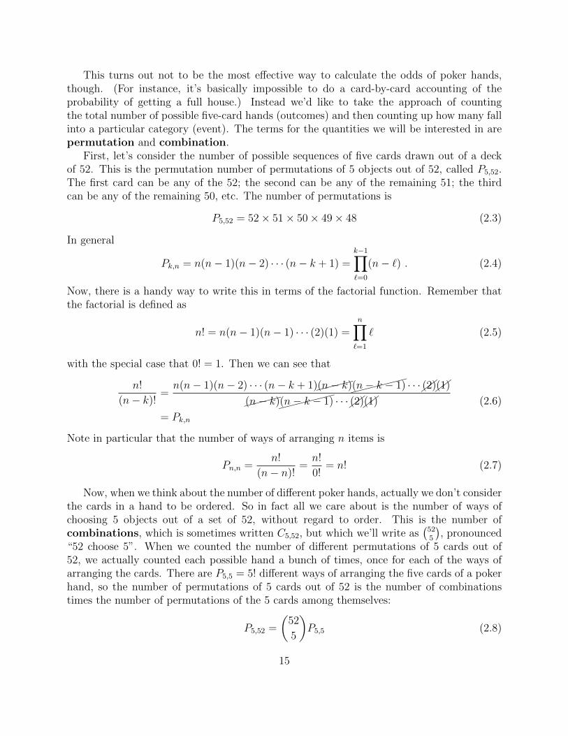
This turns out not to be the most effective way to calculate the odds of poker hands,though. (For instance, it’s basically impossible to do a card-by-card accounting of theprobability of getting a full house.) Instead we’d like to take the approach of countingthe total number of possible five-card hands (outcomes) and then counting up how many fallinto a particular category (event). The terms for the quantities we will be interested in arepermutation and combination.

First, let’s consider the number of possible sequences of five cards drawn out of a deckof 52. This is the permutation number of permutations of 5 objects out of 52, called P5,52.The first card can be any of the 52; the second can be any of the remaining 51; the thirdcan be any of the remaining 50, etc. The number of permutations is

P5,52 = 52× 51× 50× 49× 48 (2.3)

In general

Pk,n = n(n− 1)(n− 2) · · · (n− k + 1) =k−1∏`=0

(n− `) . (2.4)

Now, there is a handy way to write this in terms of the factorial function. Remember thatthe factorial is defined as

n! = n(n− 1)(n− 1) · · · (2)(1) =n∏

`=1

` (2.5)

with the special case that 0! = 1. Then we can see that

n!

(n− k)!=

n(n− 1)(n− 2) · · · (n− k + 1)����(n− k)������(n− k − 1) · · ·��(2)��(1)

����(n− k)������(n− k − 1) · · ·��(2)��(1)

= Pk,n

(2.6)

Note in particular that the number of ways of arranging n items is

Pn,n =n!

(n− n)!=

n!

0!= n! (2.7)

Now, when we think about the number of different poker hands, actually we don’t considerthe cards in a hand to be ordered. So in fact all we care about is the number of ways ofchoosing 5 objects out of a set of 52, without regard to order. This is the number ofcombinations, which is sometimes written C5,52, but which we’ll write as

(525

), pronounced

“52 choose 5”. When we counted the number of different permutations of 5 cards out of52, we actually counted each possible hand a bunch of times, once for each of the ways ofarranging the cards. There are P5,5 = 5! different ways of arranging the five cards of a pokerhand, so the number of permutations of 5 cards out of 52 is the number of combinationstimes the number of permutations of the 5 cards among themselves:

P5,52 =

(52

5

)P5,5 (2.8)

15

The factor of P5,5 = 5! is the factor by which we overcounted, so we divide by it to get(52

5

)=

P5,52

P5,5

=52!

47!5!= 2598960 (2.9)

or in general (n

k

)=

n!

(n− k)!k!(2.10)

So to return to the question of the odds of getting five hearts, there are(525

)different

poker hands, and(135

)different hands of all hearts (since there are 13 hearts in the deck),

which means the probability of the event A = ♥♥♥♥♥ is

P (A) =N(A)

N=

(135

)(525

) =13!8!5!52!47!5!

=13!47!

8!52!=

(13)(12)(11)(10)(9)

(52)(51)(50)(49)(48)(2.11)

which is of course what we calculated before. Numerically, P (A) ≈ 4.95 × 10−4, while1/45 ≈ 9.77× 10−4. The odds of getting any flush are four times the odds of getting an allheart flush, i.e., 1.98× 10−3.

Actually, if we want to calculate the odds of getting a flush, we have over-counted some-what, since we have also included straight flushes, e.g., 4♥-5♥-6♥-7♥-8♥. If we want tocount only hands which are flushes, we need to subtract those. Since aces can count aseither high or low, there are ten different all-heart straight flushes, which means the numberof different all-heart flushes which are not straight flushes is(

13

5

)− 10 =

13!

8!5!− 10 = 1287− 10 = 1277 (2.12)

and the probability of getting an all-heart flush is 4.92× 10−4, or 1.97× 10−3 for any flush.Exercise: work out the number of possible straights and therefore the odds of getting a

straight.

Practice Problems

2.5, 2.9, 2.13, 2.17, 2.29, 2.33, 2.43

16

Thursday 7 March 2013

3 Conditional Probabilities and Tree Diagrams

“Conditional Risk” http://xkcd.com/795/

3.1 Example: Odds of Winning at Craps

Although there are an infinite number of possible outcomes to a craps game, we can stillcalculate the probability of winning.

First, the sample space can be divided up into mutually exclusive events based on theresult of the first roll:

17

Event Probability Result of game

2, 3 or 12 on 1st roll 1+2+136

= 436≈ 11.1% lose

7 or 11 on 1st roll 6+236

= 836≈ 22.2% win

4 or 10 on 1st roll 3+336

= 636≈ 16.7% ???

5 or 9 on 1st roll 4+436

= 836≈ 22.2% ???

6 or 8 on 1st roll 5+536

= 1036≈ 27.8% ???

The last three events each contain some outcomes that correspond to winning, and somethat correspond to losing. We can figure out the probability of winning if, for example, youroll a 4 initially. Then you will win if another 4 comes up before a 7, and lose if a 7 comesup before a 4. On any given roll, a 7 is twice as likely to come up as a 4 (6/36 vs 3/36), sothe odds are 6/9 = 2/3 ≈ 66.7% that you will roll a 7 before a 4 and lose. Thus the odds oflosing after starting with a 4 are 66.7%, while the odds of winning after starting with a 4 are33.3%. The same calculation applies if you get a 10 on the first roll. This means that the6/36 ≈ 16.7% probability of rolling a 4 or 10 initially can be divided up into a 4/36 ≈ 11.1%probability to start with a 4 or 10 and eventually lose, and a 2/36 ≈ 5.6% probability tostart with a 4 or 10 and eventually win.

We can summarize this branching of probabilities with a tree diagram:

The probability of winning given that you’ve rolled a 4 or 10 initially is an example of aconditional probability. If A is the event “roll a 4 or 10 initially” and B is the event “win

18

the game”, we write the conditional probability for event B given that A occurs as P (B|A).We have argued that the probability for both A and B to occur, P (A ∩ B), should be theprobability of A times the conditional probability of B given A, i.e.,

P (A ∩B) = P (B|A)P (A) (3.1)

We can use this to fill out a table of probabilities for different sets of outcomes of a crapsgame, analogous to the tree diagram.

A P (A) B P (B|A) P (A ∩B) = P (B|A)P (A)

2, 3 or 12 on 1st roll .111 lose 1 .1117 or 11 on 1st roll .222 win 1 .222

4 or 10 on 1st roll .167lose .667 .111win .333 .056

5 or 9 on 1st roll .222lose .6 .133win .4 .089

6 or 8 on 1st roll .278lose .545 .152win .455 .126

Since the rows all describe disjoint events whose union is the sample space S, we can addthe probabilities of winning and find that

P (win) ≈ .222 + .056 + .089 + .126 ≈ .493 (3.2)

andP (lose) ≈ .111 + .111 + .133 + .152 ≈ .507 (3.3)

3.2 Definition of Conditional Probability

We’ve motivated the concept of conditional probability and applied it via (3.1). In fact, froma formal point of view, conditional probability is defined as

P (B|A) =P (A ∩B)

P (A). (3.4)

We actually used that definition in another context above without realizing it, when we werecalculating the probability of rolling a 7 before rolling a 4. We know that P (7) = 6/36 andP (4) = 3/36 on any given roll. The probability of rolling a 7 given that the game ends onthat throw is

P (7|7 ∪ 4) =P (7)

P (7 ∪ 4)=

P (7)

P (7) + P (4)=

6/36

9/36=

6

9(3.5)

We calculated that using the definition of conditional probability.

19

3.3 Independence

We will often say that two events A and B are independent, which means that the probabilityof A happening is the same whether or not B happens. This can be stated mathematicallyin several equivalent ways:

1. P (A|B) = P (A)

2. P (B|A) = P (B)

3. P (A ∩B) = P (A)P (B)

The first two tie most obviously to the notion of independence (the probability of A given Bis the same as the probability of A), but the third is more convenient. To show that they’reequivalent, suppose that P (A ∩B) = P (A)P (B). In that case, it’s easy to show

P (A|B) =P (A ∩B)

P (B)=

P (A)���P (B)

���P (B)= P (A) if P (A ∩B) = P (A)P (B) (3.6)

The symmetrical definition also works even if P (A) or P (B) are zero, and it extends obviouslyto more than two events:

A, B, and C are mutually independent ≡ P (A ∩B ∩ C) = P (A)P (B)P (C) (3.7)

4 Bayes’s Theorem

Some of the arguments in this section are adapted fromhttp: // yudkowsky. net/ rational/ bayes

which gives a nice explanation of Bayes’s theorem.The laws of probability are pretty good at predicting how likely something is to happen

given certain underlying circumstances. But often what you really want to know is the op-posite: given that some thing happened, what were the circumstances? The classic exampleof this is a test for a disease.

Suppose that one one-thousandth of the population has a disease. There is a test thatcan detect the disease, but it has a 2% false positive rate (on average one out of fifty healthypeople will test positive) and as 1% false negative rate (on average one out of one hundredsick people will test negative). The question we ultimately want to answer is: if someonegets a positive test result, what is the probability that they actually have the disease. Note,it is not 98%!

4.1 Approach Considering a Hypothetical Population

The standard treatment of Bayes’s Theorem and the Law of Total Probability can be sortof abstract, so it’s useful to keep track of what’s going on by considering a hypothetical

20

population which tracks the various probabilities. So, assume the probabilities arise froma population of 100,000 individuals. Of those, one one-one-thousandth, or 100, have thedisease. The other 99,900 do not. The 2% false positive rate means that of the 99,900healthy individuals, 2% of them, or 1,998, will test positive. The other 97,902 will testnegative. The 1% false negative rate means that of the 100 sick individuals, one will testnegative and the other 99 will test positive. So let’s collect this into a table:

Positive Negative Total

Sick 99 1 100Healthy 1,998 97,902 99,900

Total 2,097 97,903 100,000

(As a reminder, if we choose a sample of 100,000 individuals out of a larger population, wewon’t expect to get exactly this number of results, but the 100,000-member population is auseful conceptual construct.)

Translating from numbers in this hypothetical population, we can confirm that it capturesthe input information:

P (sick) =100

100, 000= .001 (4.1a)

P (positive|healthy) =1, 998

99, 900= .02 (4.1b)

P (negative|sick) =1

100= .01 (4.1c)

But now we can also calculate what we want, the conditional probability of being sick givena positive result. That is the fraction of the total number of individuals with positive testresults that are in the “sick and positive” category:

P (sick|positive) =99

2, 097≈ .04721 (4.2)

or about 4.7%.Note that we can forego the artificial construct of a 100,000-member hypothetical pop-

ulation. If we divide all the numbers in the table by 100,000, they become probabilities forthe corresponding events. For example,

P (sick ∩ positive) =99

100, 000= .00099

That is the approach of the slightly more axiomatic (and general) method described in thenext section.

21

4.2 Approach Using Axiomatic Probability

The quantity we’re looking for (the probability of being sick, given a positive test result) isa conditional probability. To evaluate it, we need to define some events about which we’lldiscuss the probability. First, consider the events

A1 ≡ “individual has the disease” (4.3a)

A2 ≡ “individual does not have the disease” (4.3b)

These make a mutually exclusive, exhaustive set of events, i.e., A1∩A2 = ∅ and A1∩A2 = S.(We call them A1 and A2 because in a more general case there might be more than two eventsin the mutually exclusive, exhaustive set.) We are told in the statement of the problem thatone person in 1000 has the disease, which means that

P (A1) = .001 (4.4a)

P (A2) = 1− P (A1) = .999 (4.4b)

(4.4c)

Now consider the events associated with the test:

B ≡ “individual tests positive” (4.5a)

B′ ≡ “individual tests negative” (4.5b)

(We call them B and B′ because we will focus more on B.) The 2% false positive and 1%false negative rates tell us

P (B|A2) = .02 (4.6a)

P (B′|A1) = .01 (4.6b)

Note that if we want to talk about probabilities involving B, we should use the fact that

P (B|A1) + P (B′|A1) = 1 (4.7)

to state thatP (B|A1) = 1− P (B′|A1) = .99 (4.8)

Now we can write down the quantity we actually want, using the definition of conditionalprobability:

P (A1|B) =P (A1 ∩B)

P (B)(4.9)

Now, we don’t actually have an expression for P (A1 ∩ B) or P (B) yet. The fundamentalthings we know are

P (A1) = .001 (4.10a)

P (A2) = .999 (4.10b)

P (B|A2) = .02 (4.10c)

P (B|A1) = .99 (4.10d)

22

However, we know how to calculate P (A1∩B) and P (B) from the things we do know. First,to get P (A1 ∩B), we can notice that we know P (B|A1) and P (A1), so we can solve

P (B|A1) =P (A1 ∩B)

P (A1)(4.11)

forP (A1 ∩B) = P (B|A1)P (A1) = (.99)(.001) = .00099 (4.12)

Logically, the probability of having the disease and testing positive for it is the probabilityof having the disease in the first place times the probability of testing positive, given thatyou have the disease.

Since we know P (B|A2) and P (A2) we can similarly calculate the probability of nothaving the disease but testing positive anyway:

P (A2 ∩B) = P (B|A2)P (A2) = (.02)(.999) = .01998 (4.13)

But now we have enough information to calculate P (B), since the overall probability oftesting positive for the disease has to be the probability of having the disease and testingpositive plus the probability of not having the disease and testing positive:

P (B) = P (A1 ∩B) + P (A2 ∩B) = .00099 + .01998 = .02097 (4.14)

This is an application of the Law of total probability, which says, in the more general case ofk mutually exclusive, exhaustive events A1, . . . , Ak,

P (B) = P (B ∩ A1) + · · ·+ P (B ∩ Ak) = P (B|A1)P (A1) + · · ·+ P (B|Ak)P (Ak) (4.15)

Now we are ready to calculate

P (A1|B) =P (A1 ∩B)

P (B)=

.0099

.02097≈ .04721 (4.16)

So only about 4.7% of people who test positive have the disease. It’s a lot more than one ina thousand, but a lot less than 99%.

This is an application of Bayes’s theorem, which says

P (A1|B) =P (A1 ∩B)

P (B)=

P (B|A1)P (A1)

P (B|A1)P (A1) + P (B|A2)P (A2)(4.17)

or, for k mutually exclusive, exhaustive alternatives,

P (A1|B) =P (B|A1)P (A1)∑ki=1 P (B|Ai)P (Ai)

(4.18)

Practice Problems

2.45, 2.59, 2.63, 2.67, 2.71, 2.105 parts a & b

23