Probabilistic Reliability Analysis of Electric Power

University of Wisconsin MilwaukeeUWM Digital Commons

Theses and Dissertations

August 2016

Probabilistic Reliability Analysis of Electric PowerSystems with Smart Grid Technologies and WaterDistribution Networks: Modeling, Assessment,and ComparisonRuosong XiaoUniversity of Wisconsin-Milwaukee

Follow this and additional works at: https://dc.uwm.edu/etdPart of the Civil Engineering Commons, and the Electrical and Electronics Commons

This Thesis is brought to you for free and open access by UWM Digital Commons. It has been accepted for inclusion in Theses and Dissertations by anauthorized administrator of UWM Digital Commons. For more information, please contact [email protected].

Recommended CitationXiao, Ruosong, "Probabilistic Reliability Analysis of Electric Power Systems with Smart Grid Technologies and Water DistributionNetworks: Modeling, Assessment, and Comparison" (2016). Theses and Dissertations. 1322.https://dc.uwm.edu/etd/1322

https://dc.uwm.edu/?utm_source=dc.uwm.edu%2Fetd%2F1322&utm_medium=PDF&utm_campaign=PDFCoverPages

https://dc.uwm.edu/etd?utm_source=dc.uwm.edu%2Fetd%2F1322&utm_medium=PDF&utm_campaign=PDFCoverPages

https://dc.uwm.edu/etd?utm_source=dc.uwm.edu%2Fetd%2F1322&utm_medium=PDF&utm_campaign=PDFCoverPages

http://network.bepress.com/hgg/discipline/252?utm_source=dc.uwm.edu%2Fetd%2F1322&utm_medium=PDF&utm_campaign=PDFCoverPages

http://network.bepress.com/hgg/discipline/270?utm_source=dc.uwm.edu%2Fetd%2F1322&utm_medium=PDF&utm_campaign=PDFCoverPages

https://dc.uwm.edu/etd/1322?utm_source=dc.uwm.edu%2Fetd%2F1322&utm_medium=PDF&utm_campaign=PDFCoverPages

mailto:[email protected]

PROBABILISTIC RELIABILITY ANALYSIS OF ELECTRIC POWER SYSTEMS WITH

SMART GRID TECHNOLOGIES AND WATER DISTRIBUTION NETWORKS:

MODELING, ASSESSMENT, AND COMPARISON

by

Ruosong Xiao

A Thesis Submitted in

Partial Fulfillment of the

Requirements for the Degree of

Master of Science

in Engineering

at

The University of Wisconsin-Milwaukee

August 2016

ii

ABSTRACT

PROBABILISTIC RELIABILITY ANALYSIS OF ELECTRIC POWER SYSTEMS WITH

SMART GRID TECHNOLOGIES AND WATER DISTRIBUTION NETWORKS:

MODELING, ASSESSMENT, AND COMPARISON

by

Ruosong Xiao

The University of Wisconsin-Milwaukee, 2016

Under the Supervision of Dr. Lingfeng Wang

With the rapid growth of population, the modern human society is becoming more and more

dependent on the proper operation of critical infrastructures - the interconnected electrical power

system, the drinking water distribution and supply system, the natural gas transmission and

distribution system, and so forth. It has become an important issue to maintain reliable functions

of these critical systems. As a result, comprehensive reliability evaluation is highly needed to

quantify their reliability in an objective manner. Conventionally, deterministic criteria were used

in reliability evaluations. However, it lacked the ability to model and quantify the stochastic

nature of system behaviors such as component failures. In light of these facts, this thesis deploys

probabilistic methodologies for conducting quantitative reliability modeling and assessment for

nation’s critical infrastructures including electrical power networks incorporating smart grid

technologies and water distribution networks.

Power system operators are faced with the increasingly complicated operating conditions in bulk

power systems. Yet due to the huge investment needed to build new power delivery facilities,

cost-effective solutions such as new operational strategies are becoming more attractive and

viable in recent years. Optimal transmission switching (OTS) and dynamic thermal rating (DTR)

iii

are two such technologies which offer a potential solution to improving the power system

reliability by more fully utilizing the existing power delivery assets. In this thesis, these two

technologies are first discussed, which are then incorporated into the power system reliability

evaluation procedure. Case studies are conducted on modified RTS-79 and RTS-96 systems

using MATLAB and IBM CPLEX. The obtained simulation results have shown that with the

enforcement of either OTS or DTR technology, the overall system reliability can be improved,

and system reliability can be further improved if both technologies are enforced.

The growing urban population has brought great stress to the aging drinking water distribution

systems. It is becoming more challenging to maintain a reliable drinking water distribution

system so as to meet the growing water demand. Thus, a comprehensive reliability evaluation of

the aging water delivery infrastructure is of critical importance to enable informed decision-

making in asset management of the potable water sector. This thesis also proposes a probabilistic

reliability evaluation methodology for water distribution systems based on Monte Carlo

simulation (MCS) that takes into account both mechanical failures and hydraulic failures.

Additionally, a C++ based software tool is developed to implement the proposed method. Case

studies based on two representative water distribution systems are performed to demonstrate the

effectiveness of the proposed method.

A comparison is made between the reliability analysis of electrical power systems and that of

water distribution systems. As interconnected capacitated networks, both systems share

similarities in certain aspects such as component modeling and adequacy constraints. However,

the specific features of the target systems should also be taken into consideration in the reliability

iv

modeling and evaluation in order to obtain a more comprehensive and accurate estimation of the

actual system reliability.

v

© Copyright by Ruosong Xiao, 2016

All Rights Reserved

vi

TABLE OF CONTENTS

Introduction .................................................................................................................... 1

1.1 Research Background ........................................................................................................... 1

1.2 Introduction to Reliability Analysis of Electric Power Systems Incorporating Cost-effective

Smart Grid Technologies ............................................................................................................ 3

1.2.1 Dynamic Thermal Rating ............................................................................................... 4

1.2.2 Optimal Transmission Switching ................................................................................... 5

1.3 Introduction to Reliability Analysis of Water Distribution Networks .................................. 6

1.4 Research Objectives and Thesis Layout ............................................................................... 7

Bulk Power System Reliability Analysis Considering DTR and OTS Techniques ....... 9

2.1 Introduction ........................................................................................................................... 9

2.2 Methodology of OHL Dynamic Thermal Rating ................................................................. 9

2.3 Methodology of Optimal Transmission Switching ............................................................. 12

2.4 Reliability Evaluation Framework Incorporating DTR and OTS ....................................... 15

2.5 Case Studies ........................................................................................................................ 18

2.6 Conclusions ......................................................................................................................... 26

Reliability Evaluation of Drinking Water Distribution Systems Using Monte Carlo

Simulation ..................................................................................................................................... 27

3.1 Introduction ......................................................................................................................... 27

3.2 Reliability Evaluation Background ..................................................................................... 27

3.3 Methodology of Reliability Evaluation of Drinking Water Distribution System ............... 30

3.4 Case Studies ........................................................................................................................ 33

3.5 Conclusions ......................................................................................................................... 42

vii

Discussions, Conclusions and Future Work ................................................................. 43

4.1 Similarities between Reliability Analysis of the Electrical Power System and the Water

Distribution System .................................................................................................................. 43

4.2 Differences between Reliability Analysis of Electric Power System and Water Distribution

System ....................................................................................................................................... 44

4.3 Conclusions and Future Work ............................................................................................ 45

References ..................................................................................................................................... 47

viii

LIST OF FIGURES

Figure 2-1 Flowchart diagram of reliability evaluation considering OTS & DTR....................... 17

Figure 2-2 Test system A: one-line diagram of modified IEEE RTS-79 [43] .............................. 19

Figure 2-3 Hourly air temperature of Milwaukee, WI, 2010 [45] ................................................ 20

Figure 2-4 Hourly wind speed of Milwaukee, WI, 2010 [45] ...................................................... 20

Figure 2-5 Test system A: LOLP of four test scenarios ............................................................... 21

Figure 2-6 Test system A: EDNS of four test scenarios ............................................................... 21

Figure 2-7 Test system A: EENS of four test scenarios ............................................................... 22

Figure 2-8 Test system A: Times that OTS takes effect per year in the four test scenarios ......... 22

Figure 2-9 Test system B: LOLP of four test scenarios................................................................ 24

Figure 2-10 Test system B: EDNS of four test scenarios ............................................................. 24

Figure 2-11 Test system B: EENS of four test scenarios .............................................................. 25

Figure 2-12 Test system B: Times that OTS takes effect per year in the four test scenarios ....... 25

Figure 3-1 Component statuses and system states ........................................................................ 28

Figure 3-2 Flow chart of MCS based reliability evaluation ......................................................... 30

Figure 3-3 Procedure of the software tool .................................................................................... 34

Figure 3-4 Main interface of the software tool ............................................................................. 34

Figure 3-5 Test system A [50] ...................................................................................................... 35

Figure 3-6 Test system B [50] ...................................................................................................... 36

Figure 3-7 Nodal demand profiles for test system A (48 hours) .................................................. 37

Figure 3-8 Nodal demand profiles for test system B (24 hours)................................................... 37

Figure 3-9 Coefficient of variance of EWNS for test system A ................................................... 38

Figure 3-10 Coefficient of variance of EWNS for test system B ................................................. 38

ix

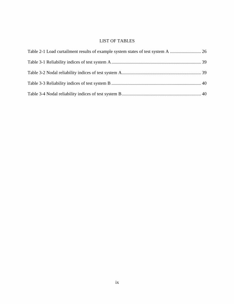
LIST OF TABLES

Table 2-1 Load curtailment results of example system states of test system A ........................... 26

Table 3-1 Reliability indices of test system A .............................................................................. 39

Table 3-2 Nodal reliability indices of test system A ..................................................................... 39

Table 3-3 Reliability indices of test system B .............................................................................. 40

Table 3-4 Nodal reliability indices of test system B ..................................................................... 40

x

ACKNOWLEDGEMENTS

It has been almost a year since I started my graduate study at the University of Wisconsin–

Milwaukee (UWM). Life here is truly exciting and full of challenges. It has been a so fascinating

experience for working with people here to do great things together. I really feel proud for the

accomplishment of this thesis in such a short time period with the guidance and help from people

around me.

I would first express my sincere gratitude to my advisor Prof. Lingfeng Wang, a man of integrity,

a scholar of dedication, and our leader of fearlessness, who always inspired me with his knowledge,

wisdom and energy, and with whom each discussion has been helpful and pleasant. I appreciate

his patient mentorship throughout my graduate study at UWM. Without his showing me the right

way I cannot imagine the accomplishment of this work. Also I would highly appreciate Prof. Jun

Zhang and Prof. Xiao Qin for serving on my thesis defense committee. Their comments and

suggestions are very helpful to improving the thesis. Thanks for their time and commitment from

their busy schedule. Thanks also go to all the professors and staff at UWM, who are always

professional, efficient and dependable.

I am also very grateful to the financial support from the funding agency. This project was in part

supported by National Science Foundation Industry/University Cooperative Research Center on

Water Equipment & Policy located at University of Wisconsin-Milwaukee and Marquette

University.

I would express my gratitude to Prof. David C. Yu and Prof. Kaigui Xie. I would always appreciate

Prof. Yu’s guidance and encouragement in my two periods of study at UWM. Prof. Kaigui Xie

xi

have led me to the field of reliability engineering. All my background about reliability engineering

and skills of programming are due to his professional guidance.

Special thanks to my labmates: Yingmeng Xiang, Jun Tan, Yunfan Zhang, Haodi Li, and Meiling

He. It has been a great experience to work with them. And I would always be grateful to

Yingmeng’s generous help with my research.

Also I want to say thanks to my friends in Milwaukee, Barbara and Bill. Without them I will not

have built such a strong relationship with the city of Milwaukee. And their elegance, integrity and

attitude towards life have been an inspiration to me in my studies here.

Finally, thanks are due to my parents, Wei Xiao and Yinghong Ren, who gave me life and a

marvelous 26 years of life by now. Your support has been such a bright dawn to me in this year

away from the hometown. You are always the closest friends, the best partners and the strongest

ally in my life.

1

Introduction

1.1 Research Background

The modern human society is highly dependent on the reliable operations of critical infrastructures

including electrical power systems, drinking water distribution systems, sewage and drainage

systems, natural gas transmission and distribution systems, and so forth. These complex systems

serve as fundamental infrastructures to support our daily lives. Failures or malfunctions of these

systems could cause severe problems such as economic loss, public health crisis or even big panic,

riots and human deaths.

On August 14, 2003, northeastern America experienced a catastrophic wide-area blackout. It is

reported during nearly a week the blackout affected approximately 50 million people in areas of

about 61,800 MW electrical load [1]. The associated economic cost was estimated to be between

$4.5 and $8.2 billion in US [2], while gross domestic product (GDP) of the month of August in

Canada was estimated to be down by 0.7% [1].

On July 30, 2012, India experienced two severe power blackouts which were believed to be the

largest in the history. The blackouts hit 20 of 28 India’s states, and nearly 600 million people,

namely nearly half of the India’s population or 9% of the world population at that time, were left

without power supply [3]. Hospitals stopped operating, transportation lost traffic control, and

protests with riots took place in many places [4].

In 2001, North Battleford in Canada experienced a drinking water crisis during which

approximately 14,000 people were affected [5]. This outbreak has also been believed to be the

2

cause of 5,800 to 7,100 reported diarrheal illness cases at that time [6].

More recently in January 2016, a water crisis took place in Flint, Michigan when this city chose to

switch the main drinking water source from Lake Huron and Detroit River to Flint River since

April 2014. Corrosive water in Flint River impaired old aging pipelines in the local drinking water

system, releasing lead contamination in the water supply which caused severe damages to public

health and finally led to a designated state of emergency for Genesee County. As one of the results,

it was reported later that in groups of children in Flint, the blood-lead levels were found to rise

from about 2.5% to as high as 5% [7].

List of incidents related to these critical infrastructures is still growing, and all these tragedies have

led to one truth: it is becoming more critical and urgent to improve the reliability of these critical

infrastructures. However, in view of the fact that most of these infrastructures are large-scale

interconnected networks, it is commonly believed to be unrealistic to mathematically model all

aspects of these systems. Conventionally deterministic reliability criteria are adopted for the

reliability evaluation of many systems. For example, in electric power systems, the N-1 or N-z

criteria, which requires the whole power system to perform its full functionality to deliver

electricity with the demanded amount and quality in the presence of one or z component failures,

has long been used as the reliability criteria in practical system designs, planning, and operations

[8]. Similarly in drinking water distribution system, traditionally the system is designed to be, if

not completely reliable, highly dependable with deterministic reliability design guidelines – e.g.,

each demand point must be supplied by at least two supply paths or the system should maintain its

reliable operation with no more than one pump failure [9]. Research about the similar concept –

availability can also be found in [10, 11]. However, in real systems the reliability characteristics

3

of typical components, such as the widely used parameters - mean time to failures (MTTF) and

mean time to repairs (MTTR), are mostly stochastic. Deterministic criteria fail to account for these

stochastic characteristics, and therefore probabilistic reliability evaluation methodologies are

preferred in order to more comprehensively evaluate the reliability performance of critical systems

or infrastructures with high uncertainties.

In light of these considerations, this thesis adopts the probabilistic methodology to perform

reliability evaluation for both electric power systems incorporating the emerging smart grid

technologies and drinking water distribution systems.

1.2 Introduction to Reliability Analysis of Electric Power Systems Incorporating

Cost-effective Smart Grid Technologies

With the increasing uncertainties due to renewable energy resources integration, system load

uncertainties, volatile weather conditions, and so forth, electric utilities are faced with an

increasingly complex and uncertain environment for system planning and operations. In order to

maintain the desired power system reliability while making the operation more economical, power

utilities are in an urgent need of cost-effective technologies for power delivery network

enhancement. While these technologies are usually considered to be too difficult to be

implemented in practices in the past, recently with the rapid development of smart power grid,

they are becoming more and more realistic. Several such technologies are being actively

investigated in the recent years, including optimal transmission switching (OTS) [12], dynamic

thermal rating (DTR) [13], network topology optimization (NTO) [14], and so forth.

4

1.2.1 Dynamic Thermal Rating

Conventionally in the power system operation, overhead line (OHL) ratings are considered as

static quantities which are calculated in a conservative assumed condition [15, 16]. However, in

fact real ratings of OHLs are affected by the actual weather conditions. It has been reported that

line ratings could increase by 10% to 30% when they are calculated accounting for real weather

conditions. In some windy areas, this increase may even be as high as 50% [17]. Thus the DTR

technology has been deployed to calculate actual ratings of overhead lines in terms of transmission

line conductor thermal limitations based on real-time weather and conductor conditions. Various

research and field tests have already been conducted to analyze the potential benefits brought by

the DTR technology.

In early research related to DTR [18-21], algorithms for calculating the dynamic thermal rating of

OHLs are studied and examined. Field tests and simulations have proven the potential benefit of

deploying DTR and associated issues on implementing DTR in real systems are also discussed.

In [22] a practical case for DTR deployment in a UK distribution system is discussed. The DTR

prototype system is deployed over 90 km of 132 kV OHLs and serves as long-term operating

strategies.

In [15] a comparison between the current application of DTR in UK and US is made. The existing

networks, climates, load patterns and adopted standards for both of these countries are discussed

in detail, which provides very useful information on implementing DTR in practice.

5

In [23] the potential reliability benefit brought by both OHL and underground cable DTR in a

distribution system was investigated. The result not only shows the significant reliability

improvement brought by DTR, but also proves the fact that DTR enforcement on OHLs has a

greater impact than underground cables.

In [16], the economic benefits brought by enforcing DTR on a certain power system with

integrations of wind power was studied. The result shows that with the enforcement of DTR, more

wind power generation can be implemented and a great economic benefits can be brought with the

enforcement of DTR.

Furthermore in [17] the reliability performance of DTR enforced system with wind farms

integrated was examined. The simulation has been conducted on the IEEE 24-bus reliability test

network consisting of 21 DTR systems and 3 integrated wind farms. And the result shows that a

higher reliability along with a greater amount of wind power delivery can be achieved.

However, while the effect of DTR and other smart grid technologies on the overall system

reliability remains a compelling research topic, most existing literature showed only the impact of

DTR. So far, very limited studies have been performed to investigate the potential benefits and

issues when DTR and other smart grid technologies are deployed simultaneously in a power

system. Thus it remains as a very interesting, open research topic.

1.2.2 Optimal Transmission Switching

In traditional power system operations, generating units are dispatched to minimize the total

operating cost. During system operations, transmission networks are usually treated as static

6

topologies. Yet in fact, the topologies of these transmission networks could be adjusted by the

system operator in a short time period, based on this consideration OTS was proposed in order to

solve challenging problems. In [24], the mechanism of OTS was first introduced. Other goals of

deploying OTS have also been studied for reducing the cost/loss [25] and cutting costs while

satisfying the N-1 standard [26]. In [12], OTS was first formulated as a mixed integer programming

problem to optimize the dispatch cost with DC optimal power flow (DCOPF) analysis, and in [27]

OTS was extended to a multi-objective (MO) optimization problem for both minimizing

generating cost and improving system reliability. The existing literature has indicated the

significant benefits that OTS can bring to the power system. Nevertheless, the integration of OTS

and other cost-effective technologies such as DTR have not been fully explored.

1.3 Introduction to Reliability Analysis of Water Distribution Networks

Water is one of the most precious resources on earth, and the drinking water distribution system is

one of the most critical infrastructures for supporting human lives. Also, drinking water systems

in urban areas are faced with the increasing pressure of meeting the growing demand. It has been

reported in [24, 28] that by the year of 2025, most countries in the world will experience serious

problems of water supply shortage. A drinking water distribution system is a complex

interconnected system consisting of one or several water sources and a number of pipelines, valves,

reservoirs, tanks, pumps, and other components. A normal drinking water distribution system

should have the ability to fulfill the demands of all nodes within the service area with the required

pressure and desired water quality. One or more failed components may impair such ability or

even interrupt the water supply to some areas, jeopardizing human health and hindering

firefighting services, etc. Thus, it is rather urgent to maintain a reliable drinking water system in

the presence of various uncertainties. An objective reliability evaluation of drinking water

7

distribution systems is useful in enabling more informed decision making considering the aging

water delivery infrastructure.

However, comprehensive reliability evaluation of a real drinking water distribution system is a

challenging task. Conventionally, two types of failures, i.e., mechanical failures and hydraulic

failures, are taken into account in water distribution system reliability evaluation [29]. Mechanical

failures refer to the system failures due to component failures such as breakage of pipelines or loss

of pumps. Hydraulic failures refer to the system failures due to unmet user demands where the

customer demands exceed the total water system capacity [29, 30]. To model a possible hydraulic

failure, nodal demand variation curves or profiles are required. Typically, to analyze hydraulic

failures, a network analysis should be performed to determine all nodal heads and pressures.

Several useful software tools have been developed for this purpose such as KYPIPE [31] and

EPANET [32]. Various reliability studies have been conducted considering either mechanical

failures [33-35] or hydraulic failures [29, 36, 37]. In [38], both mechanical failures and hydraulic

failures are taken into consideration, yet the proposed method cannot offer a systematic reliability

performance estimation.

1.4 Research Objectives and Thesis Layout

This thesis seeks to develop and perform the probabilistic reliability evaluation method for the

power system with smart grid technologies incorporated and the drinking water distribution system.

In chapter 2 the model and the methodology for bulk power system reliability analysis

incorporating DTR and OTS will be developed. Case studies will be conducted on two test systems

to illustrate the effectiveness of the method. In chapter 3 the probabilistic method for reliability

evaluation of drinking water distribution system will be presented. The methodology starts from

8

the reliability modeling of single component and then forms a comprehensive estimation method.

A Visual C++ based simulation software tool is developed, based on which case studies are carried

out to prove the effectiveness of the method. Then, discussions, conclusions and future work will

be presented in chapter 4.

9

Bulk Power System Reliability Analysis Considering DTR

and OTS Techniques

2.1 Introduction

As previously discussed, smart grid technologies like DTR and OTS could all be potential

solutions for optimizing power system operations and improving the overall system reliability. In

this chapter the integration of these technologies into the conventional bulk power system

reliability evaluation procedure and the effects of OTS and DTR will be studied.

The rest of this chapter is organized as follows. Section of 2.2 gives a brief introduction about the

DTR methodology of OHLs. Section of 2.3 discusses model and methodology of OTS. Section of

2.4 presents the proposed reliability evaluation methodology considering OTS and DTR. Section

of 2.5 gives the case studies and results. And section of 2.6 draws the conclusion of this chapter.

2.2 Methodology of OHL Dynamic Thermal Rating

Traditional ratings of OHLs are usually calculated in an assumed conservative weather condition

where the ambient temperature is 40 °C, wind speed is 0.61m/s and full sun [39]. However, the

OHL’s rating in practical operations can be increased in some cases, such as when the ambient

temperature is lower or the wind speed is higher. Therefore, the dynamic thermal rating (DTR)

method can possibly provide the ability to loosen capacity constraints of the transmission network

and achieve an improved overall system reliability [13].

Several standards and guidelines have already been developed for deriving line ratings in terms of

conductor thermal ratings such as IEEE Standard 738 [39] and the standard stipulated by CIGRE

10

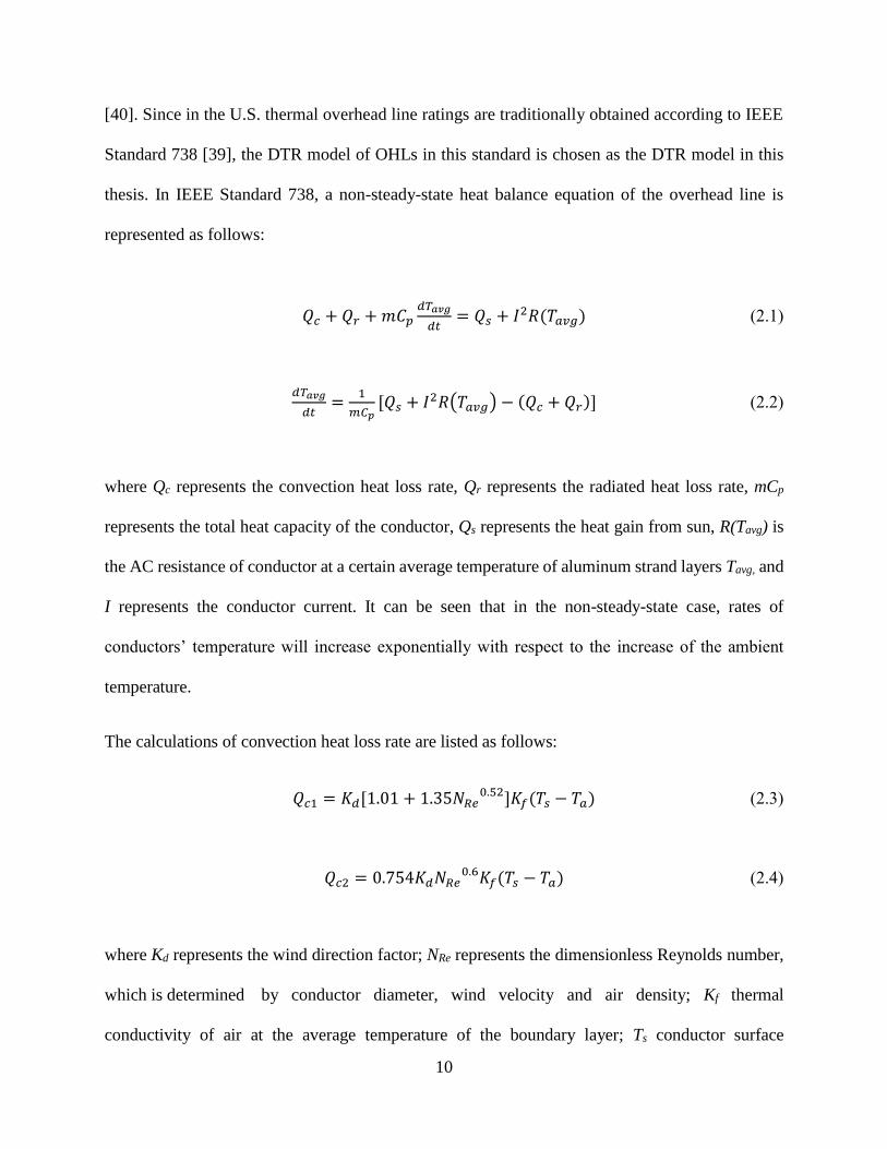
[40]. Since in the U.S. thermal overhead line ratings are traditionally obtained according to IEEE

Standard 738 [39], the DTR model of OHLs in this standard is chosen as the DTR model in this

thesis. In IEEE Standard 738, a non-steady-state heat balance equation of the overhead line is

represented as follows:

𝑄𝑐 + 𝑄𝑟 + 𝑚𝐶𝑝𝑑𝑇𝑎𝑣𝑔

𝑑𝑡= 𝑄𝑠 + 𝐼2𝑅(𝑇𝑎𝑣𝑔) (2.1)

𝑑𝑇𝑎𝑣𝑔

𝑑𝑡=

1

𝑚𝐶𝑝[𝑄𝑠 + 𝐼2𝑅(𝑇𝑎𝑣𝑔) − (𝑄𝑐 + 𝑄𝑟)] (2.2)

where Qc represents the convection heat loss rate, Qr represents the radiated heat loss rate, mCp

represents the total heat capacity of the conductor, Qs represents the heat gain from sun, R(Tavg) is

the AC resistance of conductor at a certain average temperature of aluminum strand layers Tavg, and

I represents the conductor current. It can be seen that in the non-steady-state case, rates of

conductors’ temperature will increase exponentially with respect to the increase of the ambient

temperature.

The calculations of convection heat loss rate are listed as follows:

𝑄𝑐1 = 𝐾𝑑[1.01 + 1.35𝑁𝑅𝑒0.52]𝐾𝑓(𝑇𝑠 − 𝑇𝑎) (2.3)

𝑄𝑐2 = 0.754𝐾𝑑𝑁𝑅𝑒0.6𝐾𝑓(𝑇𝑠 − 𝑇𝑎) (2.4)

where Kd represents the wind direction factor; NRe represents the dimensionless Reynolds number,

which is determined by conductor diameter, wind velocity and air density; Kf thermal

conductivity of air at the average temperature of the boundary layer; Ts conductor surface

11

temperature; Ta represents the ambient temperature. And after calculating Qc1 and Qc2, the larger

one of the two will be adopted as the value for convection heat loss rate.

The calculation of radiated heat loss rate is listed as follows:

𝑄𝑟 = 17.8𝐷𝑐𝜀[(𝑇𝑠+273

100)4 − (

𝑇𝑎+273

100)4] (2.5)

where Dc represents the conductor diameter; and ε is the emissivity factor, representing the surface

condition of the conductor.

The calculation of rate of solar heat gain is listed as follows:

𝑄𝑠 = 𝛼𝐼𝑠𝑒𝑠𝑖𝑛(𝜃)𝐴 (2.6)

where α represents the solar absorptivity factor; Ise represents the elevation corrected total solar and

sky radiated heat intensity, which is determined by total solar and sky radiated heat intensity and

solar altitude correction factor; θ represents the effective angle of incidence of the sun’s rays, which

is determined by the altitude of sun, azimuth of sun and azimuth of line; A represents the projected

area of conductor.

The calculation of conductor electrical resistance at a certain temperature will be estimated using a

liner interpolation given as follows:

𝑅(𝑇𝑎𝑣𝑔) = [𝑅(𝑇ℎ𝑖𝑔ℎ)−𝑅(𝑇𝑙𝑜𝑤)

𝑇ℎ𝑖𝑔ℎ−𝑇𝑙𝑜𝑤] (𝑇𝑎𝑣𝑔 − 𝑇𝑙𝑜𝑤) + 𝑅(𝑇𝑙𝑜𝑤) (2.7)

where R(Thigh) represents a known value of conductor resistance at a high temperature; R(Tlow)

represents a known value of conductor resistance at a low temperature. Then conductor resistance

12

value at a certain average temperature of aluminum strand layers can be calculated using this

interpolation.

Typically, for Drake ACSR, 1 hour (in most cases) is sufficient for temperatures of the conductors

to reach a steady state value [39]. The heat balance equation can then be expressed as a steady-state

form as follows:

𝑄𝑐 + 𝑄𝑟 = 𝑄𝑠 + 𝐼2𝑅(𝑇𝑎𝑣𝑔) (2.8)

Then after completing calculations of each heat loss rate and heat gain rate, the actual line rating of

OHLs in a certain hour can be expressed as:

𝐼 = √𝑄𝑐+𝑄𝑟−𝑄𝑠

𝑅(𝑇𝑎𝑣𝑔) (2.9)

In this study, a type of 795 kcmil 26/7 Drake ACSR conductor is chosen for all OHLs in the test

system. The normal operating environment of OHLs is assumed to be a weather condition with an

ambient temperature of 40 °C, full sun and a wind speed of 0.61m/s. For each hour, the ratio

between line ratings calculated using hourly environmental parameters and ratings calculated using

normal operating parameters will first be obtained. Then ratings of OHLs in the test system will be

modified as the product of this ratio and the original ratings.

2.3 Methodology of Optimal Transmission Switching

As discussed previously, OTS can be seen as a promising technology for enabling more flexible

and economical operations of electric power systems. In [12], OTS is formulated as a mixed integer

programming problem with the objective for minimizing the total generation cost. In this thesis,

13

by modifying the objective function for minimizing the total load curtailment, OTS can be

accounted for in bulk power system reliability evaluation.

With the goal of minimizing the load curtailment, the OTS problem can be modeled as follows:

min ∑ 𝑃𝐶𝑑 (2.10)

𝜃𝑛𝑚𝑖𝑛 ≤ 𝜃𝑛 ≤ 𝜃𝑛

𝑚𝑎𝑥 (2.11)

𝑃𝐺𝑔𝑚𝑖𝑛 ≤ 𝑃𝐺𝑔 ≤ 𝑃𝐺𝑔

𝑚𝑎𝑥 (2.12)

−𝑃𝐿𝑙𝑚𝑎𝑥 ≤ 𝑃𝐿𝑙 ≤ 𝑃𝐿𝑙

𝑚𝑎𝑥 (2.13)

0 ≤ 𝑃𝐶𝑑 ≤ 𝑃𝐷𝑑 (2.14)

∑ 𝑃𝐺𝑔𝑔∈𝐺𝑛 − ∑ 𝑃𝐷𝑑 𝑑∈𝐷𝑛

+ ∑ 𝑃𝐶𝑑𝑑∈𝐷𝑛 − ∑ 𝑃𝐿𝑙𝑙∈𝐿𝐹𝑛

+ ∑ 𝑃𝐿𝑙𝑙∈𝐿𝑇𝑛= 0 (2.15)

𝐵𝑙(𝜃𝑛 − 𝜃𝑚) − 𝑃𝐿𝑙 + (1 − 𝑧𝑙)𝑀 ≥ 0 (2.16)

𝐵𝑙(𝜃𝑛 − 𝜃𝑚) − 𝑃𝐿𝑙 − (1 − 𝑧𝑙)𝑀 ≤ 0 (2.17)

∑ (1 − 𝑧𝑙) ≤ 𝑀𝑙𝑙 (2.18)

where PCd is the load curtailment at load point d; θn is the voltage angle of bus n; θnmin and θn

max

is the lower and upper bounds of the angle respectively; PGg is the active power output of generator

14

g; PGgmin and PGg

max are the lower and upper power output bounds for the generator; PLl is the

power flow on line l; PLlmax is the transmission capability of line l; PDd is the load demand at load

point d; Gn is the set of generators at bus n; Dn is the set of load demands at bus n; LFn is the set

of lines of which the power flow is defined from bus n to another bus; LTn is the set of lines of

which the power flow is defined from another bus to bus n; Bl is the electrical susceptance of line

l; zl is a binary number which indicates the status of line l: if zl is 0, the line is open, otherwise it is

closed; M is a significantly large number [41]; and Ml is the maximum number of lines that are

allowed to be switched.

As shown in (2.10), the OTS problem aims to minimize the total load curtailment in the power grid

when a contingency occurs. Constraints of this programming problem are listed in expressions

(2.11)-(2.18): expressions (2.11)-(2.14) indicate the limitations associated with the bus angle,

generation output, power flow, and load curtailment, respectively; equation (2.15) ensures the

power flow balance at each bus; expressions (2.16)-(2.17) refer to the power flow of a line, which

is affected by the line switching. In expression (2.18) a limitation of maximum number of

switchable lines is defined.

Then in the reliability evaluation methodology of this thesis, OTS will be incorporated into the

reliability evaluation procedure aiming to further reduce the load curtailment, if such loss of load

exists after running an optimal power flow (OPF). For further results analysis, both the reduced

load curtailment and the original load curtailment value will be recorded, along with the number

of times that OTS actually takes effect.

15

2.4 Reliability Evaluation Framework Incorporating DTR and OTS

Based on the previous discussions about DTR and OTS, as they both have the potential to improving

the power system reliability, utilizing both technologies simultaneously could be more beneficial

to increasing the system reliability. Since DTR requires chronological weather data, sequential

Monte Carlo simulation (MCS) based reliability evaluation method will be used to tackle the

problem.

A typical sequential MCS based reliability evaluation procedure mainly contains the following

basic steps [42]. First, component reliability characteristics should be properly modeled, and the

related reliability parameters as well as the configuration data of the power system are needed. Then

system states will be randomly generated using the sequential MCS method. For each randomly

generated system state, an OPF analysis will be then conducted to calculate the amount of load

curtailment. And after a sufficient number of system states have been sampled and analyzed, based

on the sampled system states coupled with their corresponding curtailed loads, reliability indices

such as loss of load probability (LOLP), expected demand not supplied (EDNS), and expected

energy not supplied (EENS) can be calculated. These indices represent system reliability from

different perspectives.

With DTR being taken into consideration, static line ratings will be modified with hourly weather

data, then the configuration data of the system will be changed with chronologically sampled system

states thereby. And the OTS technology will take effect after running DCOPF and may affect the

curtailed load in step III. For each sampled state, if the load curtailment calculated using DCOPF is

larger than that later calculated using OTS, the load curtailment will then be updated with the

smaller value and this system state will be marked as “OTS successfully enforced” in such a case.

16

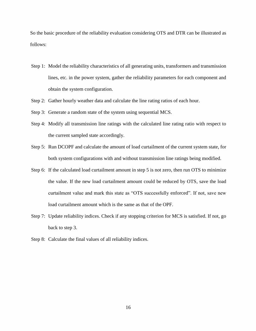
So the basic procedure of the reliability evaluation considering OTS and DTR can be illustrated as

follows:

Step 1: Model the reliability characteristics of all generating units, transformers and transmission

lines, etc. in the power system, gather the reliability parameters for each component and

obtain the system configuration.

Step 2: Gather hourly weather data and calculate the line rating ratios of each hour.

Step 3: Generate a random state of the system using sequential MCS.

Step 4: Modify all transmission line ratings with the calculated line rating ratio with respect to

the current sampled state accordingly.

Step 5: Run DCOPF and calculate the amount of load curtailment of the current system state, for

both system configurations with and without transmission line ratings being modified.

Step 6: If the calculated load curtailment amount in step 5 is not zero, then run OTS to minimize

the value. If the new load curtailment amount could be reduced by OTS, save the load

curtailment value and mark this state as “OTS successfully enforced”. If not, save new

load curtailment amount which is the same as that of the OPF.

Step 7: Update reliability indices. Check if any stopping criterion for MCS is satisfied. If not, go

back to step 3.

Step 8: Calculate the final values of all reliability indices.

17

StartStart

Gather reliability parameters of all components of the systemGather reliability parameters of all components of the system

EndEnd

Yes

No

Calculate line rating ratios with hourly weather data using DTRCalculate line rating ratios with hourly weather data using DTR

Generates a random state of system using sequential MCS Generates a random state of system using sequential MCS

Modify all transmission line ratings with the calculated ratio, with respect to the

current system state

Modify all transmission line ratings with the calculated ratio, with respect to the

current system state

Run OPF analysis for both modified and unmodified system, calculate load

curtailment amounts

Run OPF analysis for both modified and unmodified system, calculate load

curtailment amounts

Zero load curtailed?Zero load curtailed?

Run OTS, calculate the load lossRun OTS, calculate the load loss

Record load loss resultsRecord load loss results

Update reliability indexUpdate reliability index

Stop criteria satisfied?Stop criteria satisfied?

No

Yes

Calculate the final values of reliability indicesCalculate the final values of reliability indices

Load curtailed reduced?Load curtailed reduced?

No

OTS successfully

enforced times +1

OTS successfully

enforced times +1

Yes

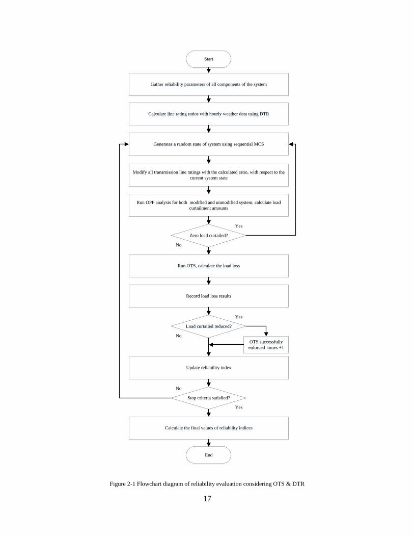
Figure 2-1 Flowchart diagram of reliability evaluation considering OTS & DTR

18

2.5 Case Studies

To illustrate the effectiveness of the proposed methodology, two systems are used as the test bulk

power systems for case studies: Test system A - IEEE RTS-79 system [43] with all capacities of

transmission components being modified to 85% of the original values in [43] (painted in Figure

2-2); Test system B - IEEE RTS-96 system [44] with all capacities of transmission components

being modified to 60% of the original values in [44]. The simulation is conducted based on

MATLAB and IBM CPLEX. Hourly weather data of Milwaukee, WI in the year 2010 [45] is used

for calculating the actual line ratings of OHLs in this thesis, which are shown in Figure 2-2 and 2-

3.

System reliability will be evaluated for the following four test scenarios:

I. Base case: original system with OPF.

II. System with OTS enforced.

III. System with DTR enforced.

IV. System with both OTS and DTR enforced.

Sequential Monte Carlo simulation time has been set to be 100 years (876,000 hours) for test

scenarios in test system A and 20 years (175,200 hours) for test scenarios in test system B. Settings

of the simulation duration will be enough to guarantee the coefficient of variation of the EDNS

index for both test systems to be less than 0.5%. And in order to analyze the exact benefits brought

by DTR, OTS or the combination of these two technologies while eliminating the uncertainty

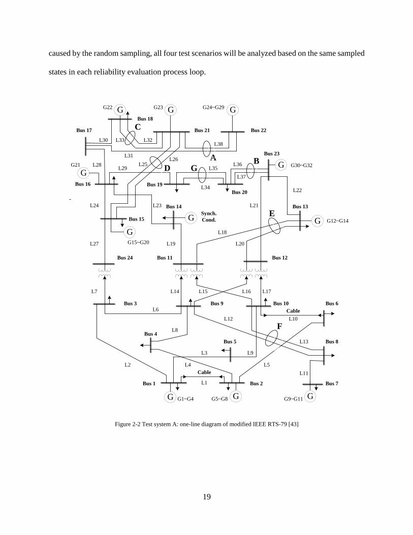
19

caused by the random sampling, all four test scenarios will be analyzed based on the same sampled

states in each reliability evaluation process loop.

G

G GBus 18

A

Bus 21 Bus 22

Bus 23

Bus 17

Bus 16 Bus 19

Bus 20

Bus 15

Bus 14 Bus 13

Bus 24 Bus 11 Bus 12

Bus 3 Bus 9 Bus 10 Bus 6

Bus 4

Bus 5 Bus 8

Bus 1 Bus 2 Bus 7

G

G

G

G G

G G G

B

C

D

E

F

G

Cable

Cable

Synch.

Cond.

L1

L2

L3

L4 L5

L6

L7

L8

L9

L10

L11

L12

L13

L14 L15 L16 L17

L18

L19 L20

L21

L22

L23L24

L25L26

L27

L28L29

L30

L31

L32L33

L34

L35L36

L37

L38

G1~G4 G5~G8 G9~G11

G12~G14

G15~G20

G21

G22 G23 G24~G29

G30~G32

Figure 2-2 Test system A: one-line diagram of modified IEEE RTS-79 [43]

20

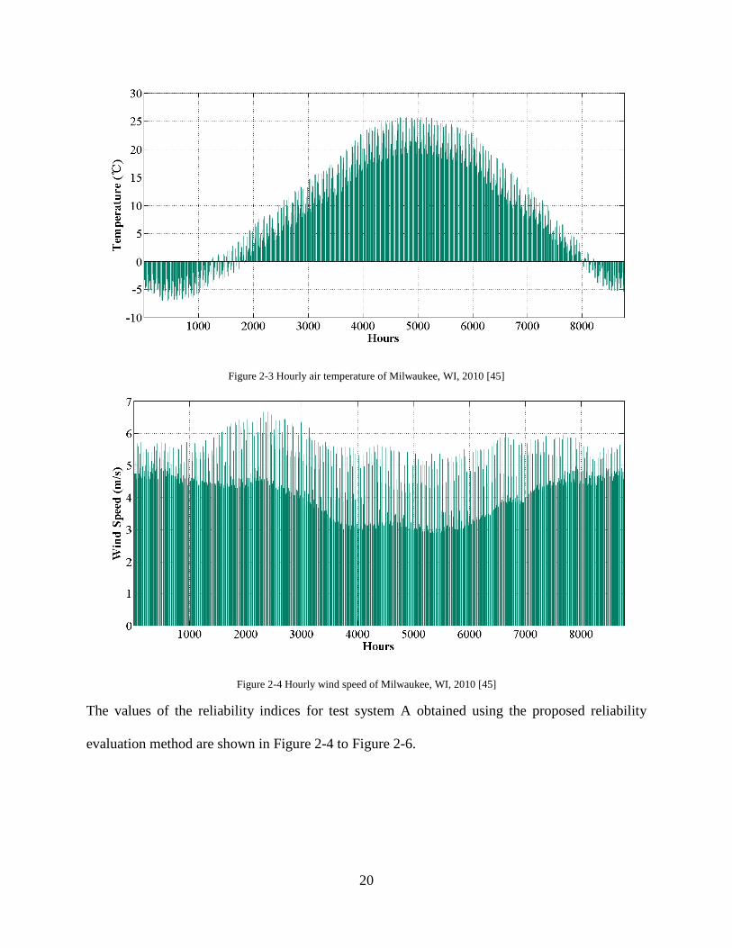
Figure 2-3 Hourly air temperature of Milwaukee, WI, 2010 [45]

Figure 2-4 Hourly wind speed of Milwaukee, WI, 2010 [45]

The values of the reliability indices for test system A obtained using the proposed reliability

evaluation method are shown in Figure 2-4 to Figure 2-6.

21

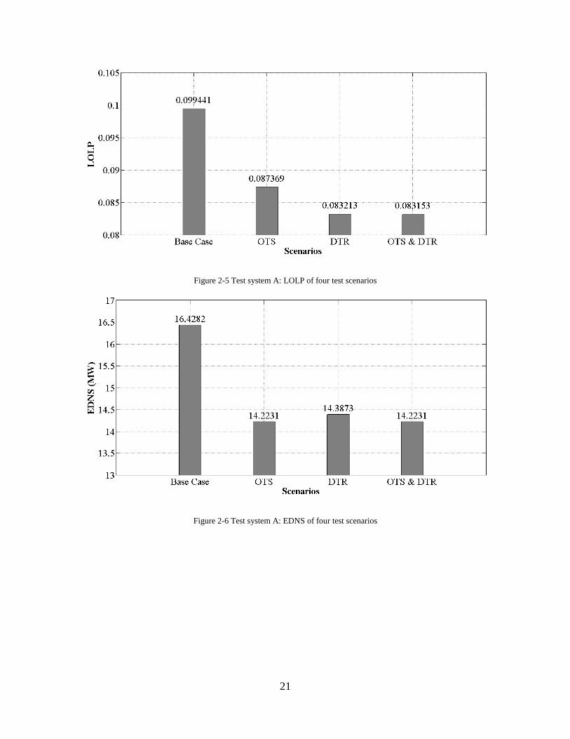
Figure 2-5 Test system A: LOLP of four test scenarios

Figure 2-6 Test system A: EDNS of four test scenarios

22

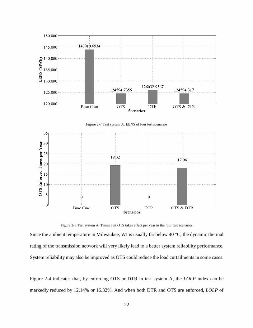
Figure 2-7 Test system A: EENS of four test scenarios

Figure 2-8 Test system A: Times that OTS takes effect per year in the four test scenarios

Since the ambient temperature in Milwaukee, WI is usually far below 40 °C, the dynamic thermal

rating of the transmission network will very likely lead to a better system reliability performance.

System reliability may also be improved as OTS could reduce the load curtailments in some cases.

Figure 2-4 indicates that, by enforcing OTS or DTR in test system A, the LOLP index can be

markedly reduced by 12.14% or 16.32%. And when both DTR and OTS are enforced, LOLP of

23

the system will be further decreased by 16.38%. Figure 2-5 and 2-6 list the system EDNS and

EENS results. The results indicate that by enforcing OTS, DTR, and both OTS and DTR, the

system EDNS index will decrease by 13.42%, 12.42%, and 13.42%, respectively.

As previously described, in the reliability evaluation methodology of this study, OTS takes effect

only when the amount of the optimized load curtailment using OTS is reduced with respect to the

original load curtailment amount. Figure 2-7 shows the average number of times per year when

OTS takes effect. For a 100-year Monte Carlo simulation, in average OTS takes effect for 17.96

and 19.32 times per year with and without DTR enforced, respectively.

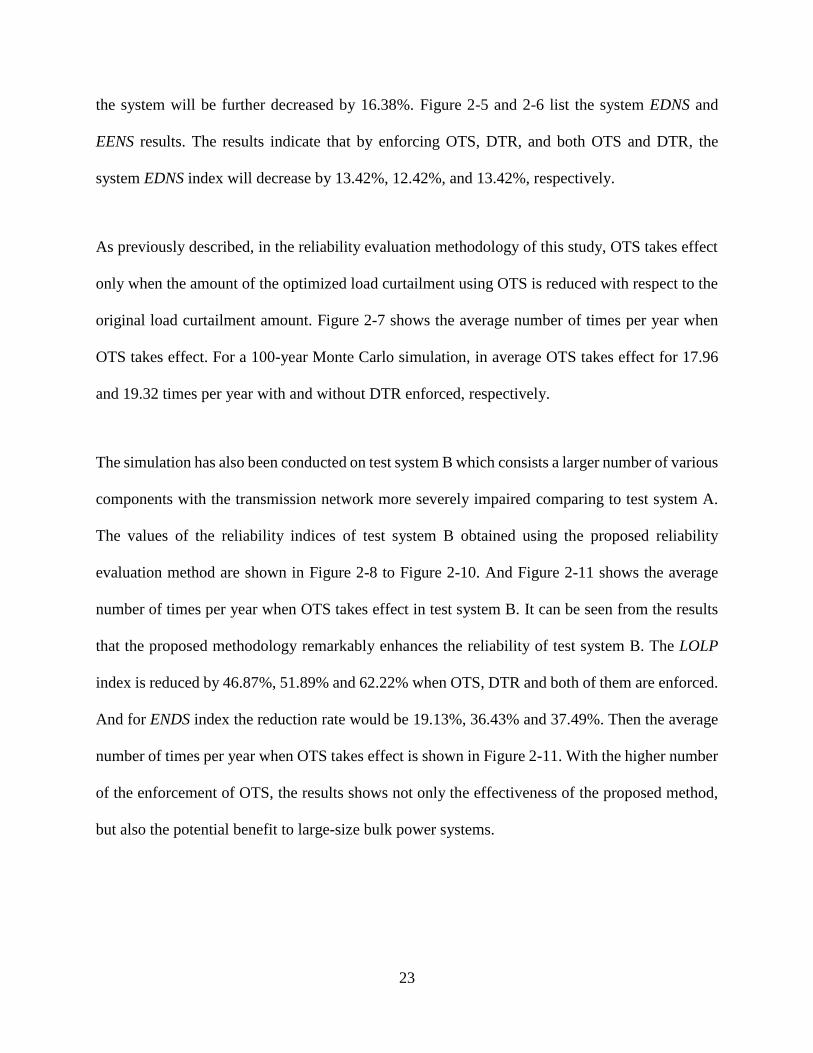
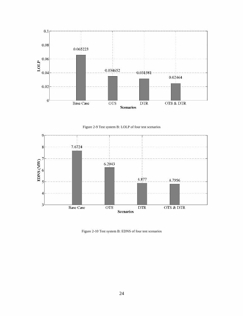
The simulation has also been conducted on test system B which consists a larger number of various

components with the transmission network more severely impaired comparing to test system A.

The values of the reliability indices of test system B obtained using the proposed reliability

evaluation method are shown in Figure 2-8 to Figure 2-10. And Figure 2-11 shows the average

number of times per year when OTS takes effect in test system B. It can be seen from the results

that the proposed methodology remarkably enhances the reliability of test system B. The LOLP

index is reduced by 46.87%, 51.89% and 62.22% when OTS, DTR and both of them are enforced.

And for ENDS index the reduction rate would be 19.13%, 36.43% and 37.49%. Then the average

number of times per year when OTS takes effect is shown in Figure 2-11. With the higher number

of the enforcement of OTS, the results shows not only the effectiveness of the proposed method,

but also the potential benefit to large-size bulk power systems.

24

Figure 2-9 Test system B: LOLP of four test scenarios

Figure 2-10 Test system B: EDNS of four test scenarios

25

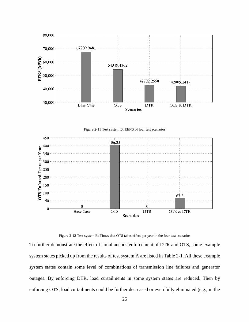
Figure 2-11 Test system B: EENS of four test scenarios

Figure 2-12 Test system B: Times that OTS takes effect per year in the four test scenarios

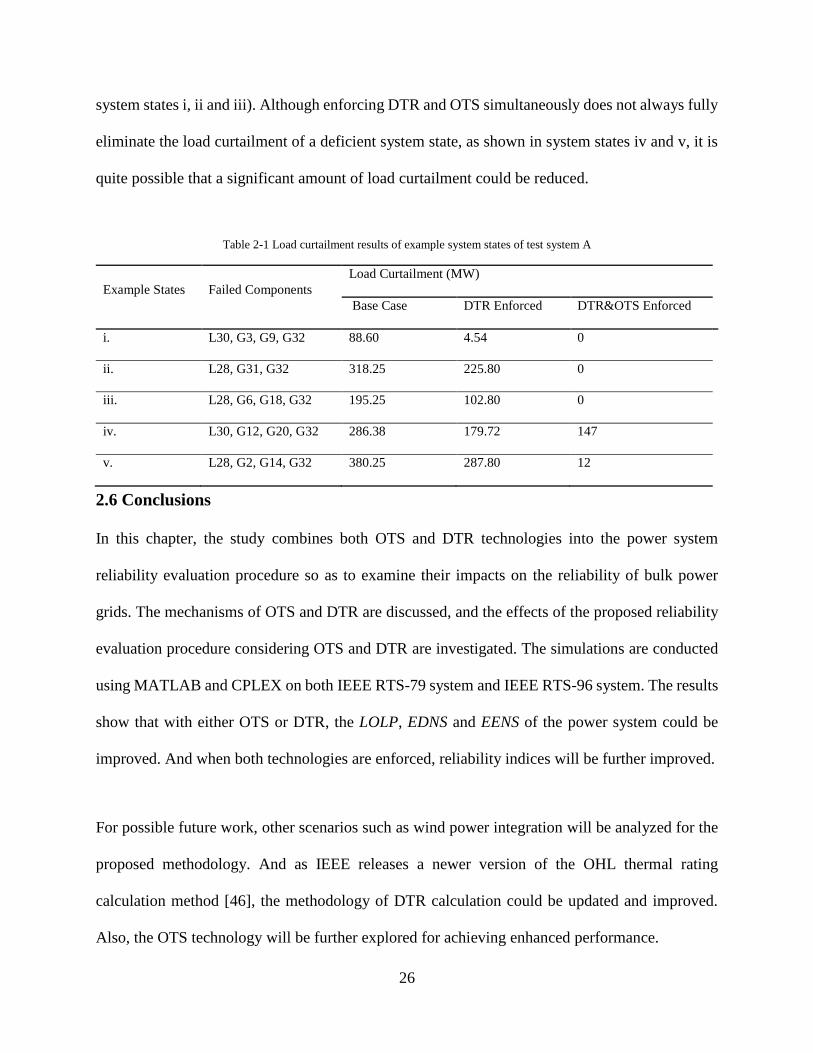
To further demonstrate the effect of simultaneous enforcement of DTR and OTS, some example

system states picked up from the results of test system A are listed in Table 2-1. All these example

system states contain some level of combinations of transmission line failures and generator

outages. By enforcing DTR, load curtailments in some system states are reduced. Then by

enforcing OTS, load curtailments could be further decreased or even fully eliminated (e.g., in the

26

system states i, ii and iii). Although enforcing DTR and OTS simultaneously does not always fully

eliminate the load curtailment of a deficient system state, as shown in system states iv and v, it is

quite possible that a significant amount of load curtailment could be reduced.

Table 2-1 Load curtailment results of example system states of test system A

Example States Failed Components

Load Curtailment (MW)

Base Case DTR Enforced DTR&OTS Enforced

i. L30, G3, G9, G32 88.60 4.54 0

ii. L28, G31, G32 318.25 225.80 0

iii. L28, G6, G18, G32 195.25 102.80 0

iv. L30, G12, G20, G32 286.38 179.72 147

v. L28, G2, G14, G32 380.25 287.80 12

2.6 Conclusions

In this chapter, the study combines both OTS and DTR technologies into the power system

reliability evaluation procedure so as to examine their impacts on the reliability of bulk power

grids. The mechanisms of OTS and DTR are discussed, and the effects of the proposed reliability

evaluation procedure considering OTS and DTR are investigated. The simulations are conducted

using MATLAB and CPLEX on both IEEE RTS-79 system and IEEE RTS-96 system. The results

show that with either OTS or DTR, the LOLP, EDNS and EENS of the power system could be

improved. And when both technologies are enforced, reliability indices will be further improved.

For possible future work, other scenarios such as wind power integration will be analyzed for the

proposed methodology. And as IEEE releases a newer version of the OHL thermal rating

calculation method [46], the methodology of DTR calculation could be updated and improved.

Also, the OTS technology will be further explored for achieving enhanced performance.

27

Reliability Evaluation of Drinking Water Distribution

Systems Using Monte Carlo Simulation

3.1 Introduction

Reliability evaluation of drinking water distribution systems remains as an important issue.

However, a comprehensive reliability estimation of such systems is difficult, and the related

studies on this topic are rather limited. A probabilistic methodology for reliability evaluation

incorporating both mechanical failures and hydraulic failures is proposed in this chapter. The

method is developed to be able to provide both system-level and node-level reliability estimations.

And a Visual C++ based software simulation tool is developed based on the proposed methodology

to enable informed decision-making.

The rest of this chapter is organized as follows. Section 3.2 presents the probabilistic reliability

evaluation background. And in section 3.3 the methodology of reliability evaluation of drinking

water distribution system is proposed. Case studies and simulation results are listed in section 3.4.

And section 3.5 draws the conclusion of this chapter.

3.2 Reliability Evaluation Background

Probabilistic reliability evaluation theory has been well established [47] and widely applied in

various fields such as electric power systems [8]. To evaluate the reliability of drinking water

distribution systems, first the status of each component within the system needs to be modeled. In

this thesis, pipes and pumps are represented by two-state models as they are physically repairable

in most conditions. As shown in Figure 3-1, “UP” status indicates the normal condition and

“DOWN” status represents the faulty condition of the component. These statuses vary with respect

28

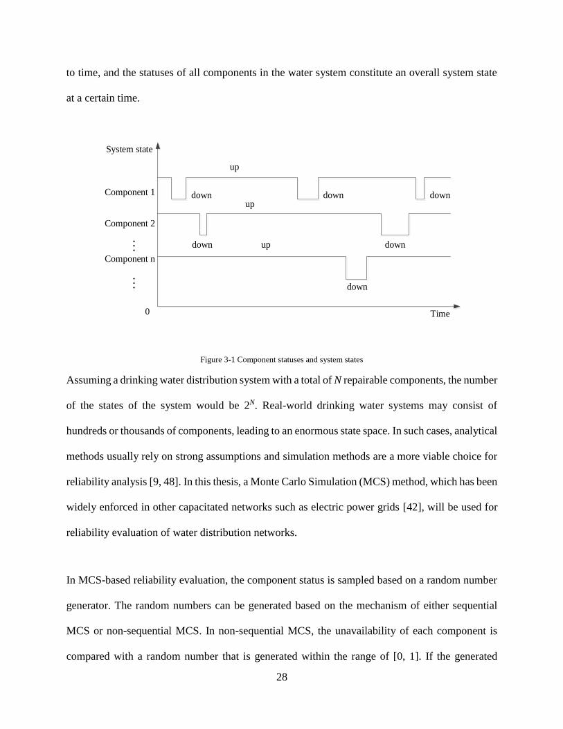
to time, and the statuses of all components in the water system constitute an overall system state

at a certain time.

Component 1

up

down

Time

System state

0

down

updown

down down down

up

Component 2

Component n

Figure 3-1 Component statuses and system states

Assuming a drinking water distribution system with a total of N repairable components, the number

of the states of the system would be 2N. Real-world drinking water systems may consist of

hundreds or thousands of components, leading to an enormous state space. In such cases, analytical

methods usually rely on strong assumptions and simulation methods are a more viable choice for

reliability analysis [9, 48]. In this thesis, a Monte Carlo Simulation (MCS) method, which has been

widely enforced in other capacitated networks such as electric power grids [42], will be used for

reliability evaluation of water distribution networks.

In MCS-based reliability evaluation, the component status is sampled based on a random number

generator. The random numbers can be generated based on the mechanism of either sequential

MCS or non-sequential MCS. In non-sequential MCS, the unavailability of each component is

compared with a random number that is generated within the range of [0, 1]. If the generated

29

random number is greater than the component unavailability, this component will be assumed to

be in the “UP” status; otherwise it is in the “DOWN” status:

𝑆𝑖 = {0 if 𝑅𝑎𝑛𝑑 > 𝑈𝑖

1 if 𝑅𝑎𝑛𝑑 ≤ 𝑈𝑖 (3.1)

where Si is the simulated status of component i, 0 represents the “UP” status and 1 represents the

“DOWN” status; Rand stands for a randomly generated number within the range of [0, 1]; and Ui

is the unavailability of component i.

In the sequential MCS, two time chains of the component (i.e., time to failure (TTF) and time to

repair (TTR)) will be randomly generated for determination of the status of the component. The

component will be assumed to be in the “UP” status within the TTF, and in the “DOWN” status

within the TTR. Then after all the TTF and TTR values are generated, system states can be

determined for each moment. The values of TTF and TTR can be calculated as follows:

𝑇𝑇𝐹 = −log (𝑅𝑎𝑛𝑑) ∙ 𝑀𝑇𝑇𝐹 (3.2)

𝑇𝑇𝑅 = −log (𝑅𝑎𝑛𝑑) ∙ 𝑀𝑇𝑇𝑅 (3.3)

where MTTF is the mean time to failure; and MTTR is the mean time to repair.

Then for each sampled system state, a network analysis will be conducted to evaluate the system

state with respect to the specified reliability criteria. After an adequate number of system states are

30

sampled and evaluated, the MCS may be halted, and the final results obtained are deemed

reasonable estimates of the desired reliability indices.

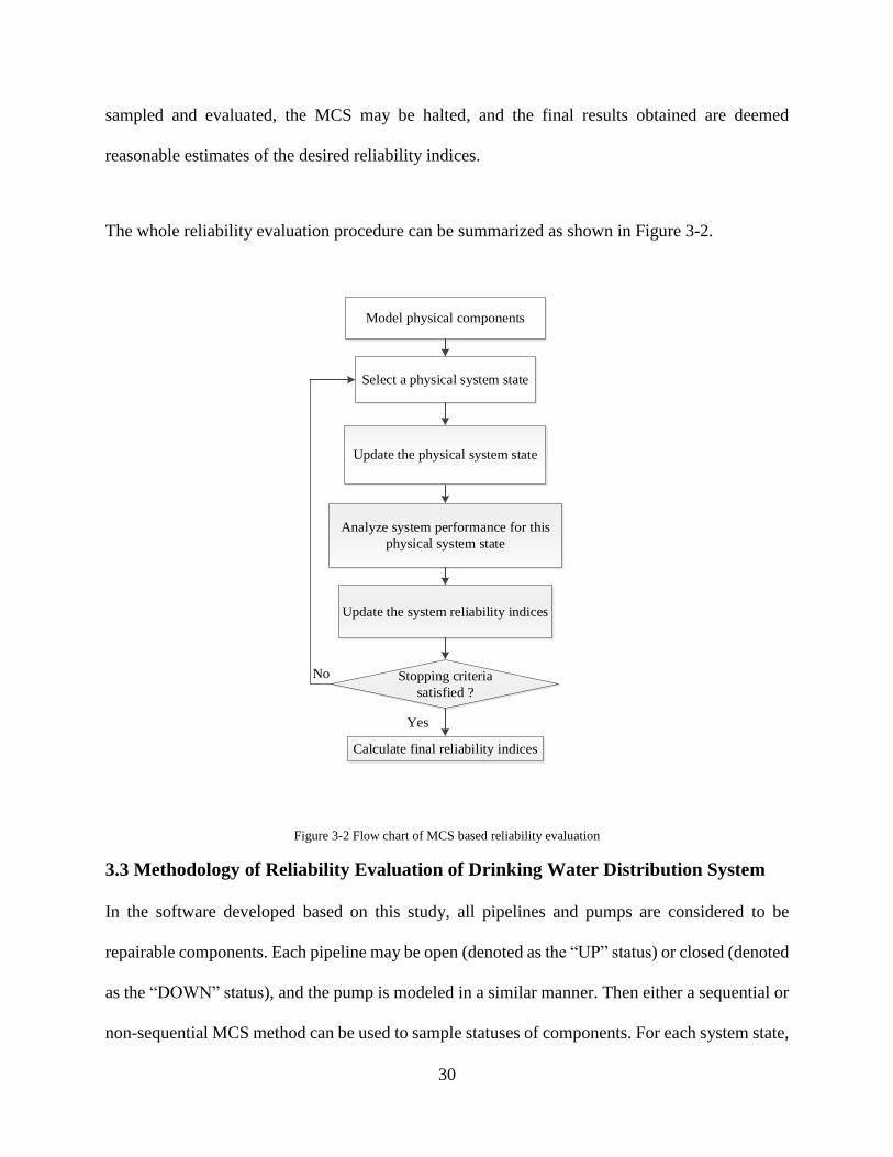
The whole reliability evaluation procedure can be summarized as shown in Figure 3-2.

Select a physical system state

Analyze system performance for this

physical system state

Update the system reliability indices

Stopping criteria

satisfied ?

Calculate final reliability indices

Model physical components

Update the physical system state

No

Yes

Figure 3-2 Flow chart of MCS based reliability evaluation

3.3 Methodology of Reliability Evaluation of Drinking Water Distribution System

In the software developed based on this study, all pipelines and pumps are considered to be

repairable components. Each pipeline may be open (denoted as the “UP” status) or closed (denoted

as the “DOWN” status), and the pump is modeled in a similar manner. Then either a sequential or

non-sequential MCS method can be used to sample statuses of components. For each system state,

31

the hydraulic simulator EPANET is integrated with the developed software for performing water

flow analysis.

Reliable water supply is dependent on the pressure, and insufficient pressure can result in water

demand loss. For each node, the actually supplied water is calculated with respect to the pressure

as follows [49]:

𝐷𝑎𝑖 = {𝐷𝑟𝑖 if 𝑃𝑐𝑖 ≥ 𝑃𝑚𝑖𝑛

𝐷𝑟𝑖√𝑃𝑐𝑖

√𝑃𝑚𝑖𝑛 if 𝑃𝑐𝑖 < 𝑃𝑚𝑖𝑛

(3.4)

where Dai is the actually supplied water at node i; Dri is the required water demand at node i; Pci

is the calculated pressure at node i; P is the threshold pressure for all nodes within the system,

which is set to be 40 psi in the following case studies.

If the minimal pressure threshold cannot be reached, the loss of nodal demand can be defined as

follows:

𝐷𝑙𝑜𝑠𝑠𝑖 = (1 −√𝑃𝑐𝑖

√𝑃𝑚𝑖𝑛)𝐷𝑟𝑖 (3.5)

where Dlossi is the loss of nodal demand at node i;

Then in this thesis, several reliability indices indicating both system-wide and nodal reliability

performance are defined in the following.

32

The percentage of unsatisfied water demand (PUWD) index is defined as follows:

𝑃𝑈𝑊𝐷 =∑ ∑ 𝐷𝑙𝑜𝑠𝑠𝑖,𝑛 𝑖𝑛

∑ ∑ 𝐷𝑟𝑖,𝑛 𝑖𝑛 (3.6)

𝑃𝑈𝑊𝐷𝑖 =∑ 𝐷𝑙𝑜𝑠𝑠𝑖,𝑛𝑛

∑ 𝐷𝑟𝑖,𝑛𝑛 (3.7)

where PUWD is the percentage of unsatisfied water demand index of the system; PUWDi is the

percentage of unsatisfied water demand of node i in the system; Dlossi,n is the nodal demand loss of

node i in the nth iteration of MCS measured in gallons per minute; and Dri,n is the water demand

at node i in the nth MCS iteration measured in gallons per minute (gpm).

The probability of loss of water service (PLWS) index is defined as follows:

𝑃𝐿𝑊𝑆 =𝑁𝑙𝑜𝑠𝑠

∑ ∙ ∑ 𝑖𝑛 (3.8)

𝑃𝐿𝑊𝑆𝑖 =𝑁𝑙𝑜𝑠𝑠𝑖

∑ ∙ ∑ 𝑖𝑛 (3.9)

where PLWS is the probability of loss of water service index of the system; PLWSi is the probability

of loss of water service index of node i within the system; Nloss is the number of system states in

which there is unsatisfied nodal demand; and Nlossi is the number of system states in which the

demand of node i is not fully satisfied.

The expected water not supplied (EWNS) index is defined as follows:

33

𝐸𝑊𝑁𝑆 =∑ ∑ 𝐷𝑙𝑜𝑠𝑠𝑖,𝑛 𝑖𝑛

∑ ∙ ∑ 𝑖𝑛 ∙ 0.5256 (3.10)

𝐸𝑊𝑁𝑆𝑖 =∑ 𝐷𝑙𝑜𝑠𝑠𝑖,𝑛𝑛

∑ ∙ ∑ 𝑖𝑛 ∙ 0.5256 (3.11)

where EWNS is the reliability index indicating the expected water not supplied in the unit of

millions of gallons per year; and EWNSi is the expected water not supplied of node i, which is

measured in millions of gallons per year.

With the quantitative reliability indices defined above, in the simulation after a reasonable number

of iterations, both the system-level and nodal reliability indices can be obtained, which indicate

the system or node level reliability characteristics of the water distribution network from different

perspectives.

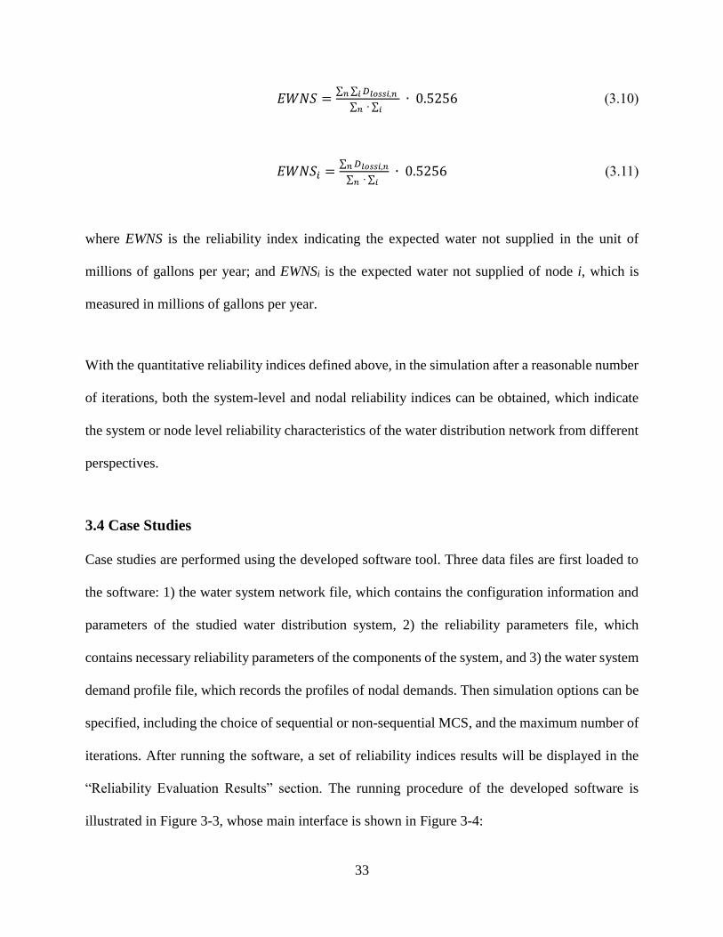
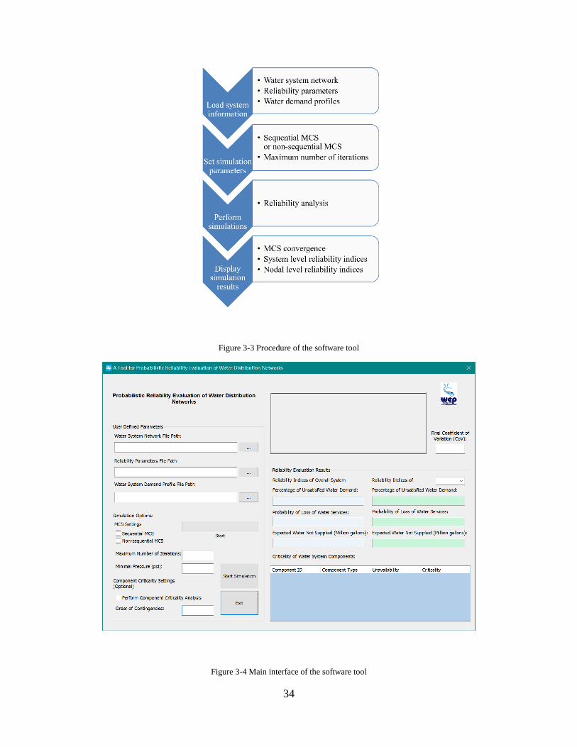
3.4 Case Studies

Case studies are performed using the developed software tool. Three data files are first loaded to

the software: 1) the water system network file, which contains the configuration information and

parameters of the studied water distribution system, 2) the reliability parameters file, which

contains necessary reliability parameters of the components of the system, and 3) the water system

demand profile file, which records the profiles of nodal demands. Then simulation options can be

specified, including the choice of sequential or non-sequential MCS, and the maximum number of

iterations. After running the software, a set of reliability indices results will be displayed in the

“Reliability Evaluation Results” section. The running procedure of the developed software is

illustrated in Figure 3-3, whose main interface is shown in Figure 3-4:

34

Figure 3-3 Procedure of the software tool

Figure 3-4 Main interface of the software tool

35

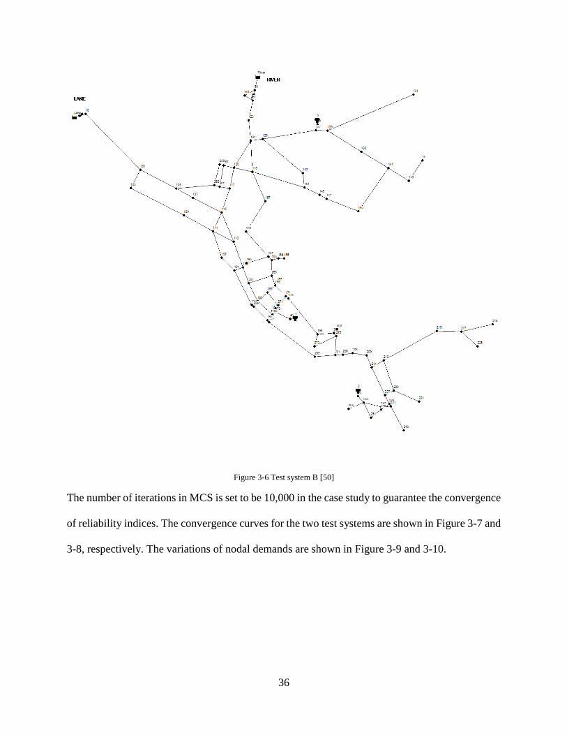
Two test systems provided by EPANET are adopted as the test systems in this thesis [50]. Test

system A comprises 40 pipes, 35 junctions and 1 tank, with a total nodal demand of 322.78 gpm.

Test system B is a larger system which comprises 117 pipes, 92 junctions, 2 pumps, 2 reservoirs

and 3 tanks, with a total nodal demand of 3,052.11 gpm. Topological diagrams of these two test

systems are shown in Figs. 5-6 and nodal demand profiles are shown in Figure 3-5 and 3-6.

Figure 3-5 Test system A [50]

1

23

4

5

6

7

8

9

10

11

12

13

14

15

16

1718

19

20

21

22

23

24

25

27

2829

3031

32

33

34

35

36

26

Pump

Station

Tank

36

Figure 3-6 Test system B [50]

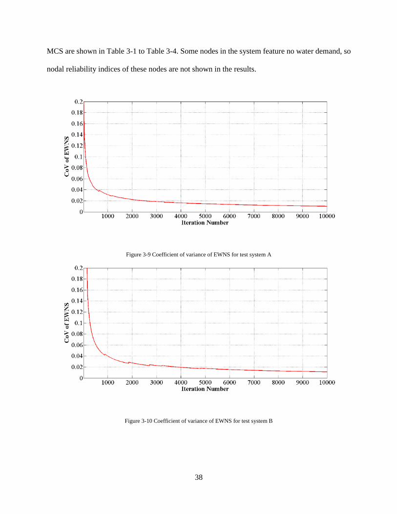
The number of iterations in MCS is set to be 10,000 in the case study to guarantee the convergence

of reliability indices. The convergence curves for the two test systems are shown in Figure 3-7 and

3-8, respectively. The variations of nodal demands are shown in Figure 3-9 and 3-10.

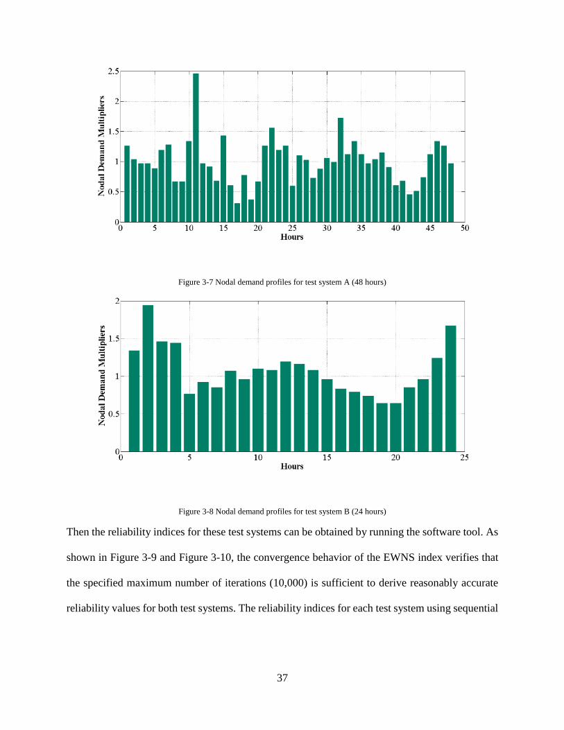
37

Figure 3-7 Nodal demand profiles for test system A (48 hours)

Figure 3-8 Nodal demand profiles for test system B (24 hours)

Then the reliability indices for these test systems can be obtained by running the software tool. As

shown in Figure 3-9 and Figure 3-10, the convergence behavior of the EWNS index verifies that

the specified maximum number of iterations (10,000) is sufficient to derive reasonably accurate

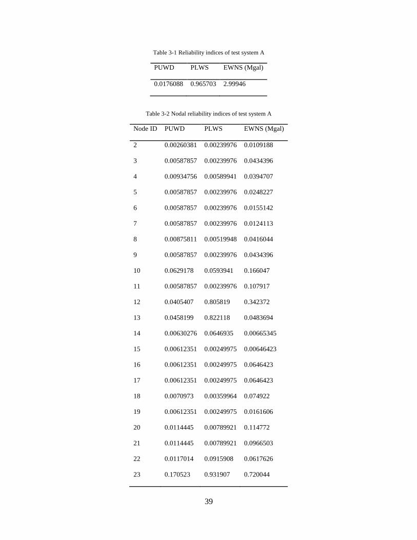
reliability values for both test systems. The reliability indices for each test system using sequential

38

MCS are shown in Table 3-1 to Table 3-4. Some nodes in the system feature no water demand, so

nodal reliability indices of these nodes are not shown in the results.

Figure 3-9 Coefficient of variance of EWNS for test system A

Figure 3-10 Coefficient of variance of EWNS for test system B

39

Table 3-1 Reliability indices of test system A

PUWD PLWS EWNS (Mgal)

0.0176088 0.965703 2.99946

Table 3-2 Nodal reliability indices of test system A

Node ID PUWD PLWS EWNS (Mgal)

2 0.00260381 0.00239976 0.0109188

3 0.00587857 0.00239976 0.0434396

4 0.00934756 0.00589941 0.0394707

5 0.00587857 0.00239976 0.0248227

6 0.00587857 0.00239976 0.0155142

7 0.00587857 0.00239976 0.0124113

8 0.00875811 0.00519948 0.0416044

9 0.00587857 0.00239976 0.0434396

10 0.0629178 0.0593941 0.166047

11 0.00587857 0.00239976 0.107917

12 0.0405407 0.805819 0.342372

13 0.0458199 0.822118 0.0483694

14 0.00630276 0.0646935 0.00665345

15 0.00612351 0.00249975 0.00646423

16 0.00612351 0.00249975 0.0646423

17 0.00612351 0.00249975 0.0646423

18 0.0070973 0.00359964 0.074922

19 0.00612351 0.00249975 0.0161606

20 0.0114445 0.00789921 0.114772

21 0.0114445 0.00789921 0.0966503

22 0.0117014 0.0915908 0.0617626

23 0.170523 0.931907 0.720044

40

24 0.00465387 0.00189981 0.0270205

25 0.176835 0.965703 0.560024

27 0.00911557 0.00819918 0.0384911

29 0.00985238 0.0089991 0.036402

30 0.0176098 0.0163984 0.0278845

31 0.00551912 0.00459954 0.0495229

32 0.00612351 0.00249975 0.054946

33 0.0301038 0.0263974 0.0238341

34 0.061021 0.0576942 0.0483123

36 0.0189981 0.0189981 0.0099854

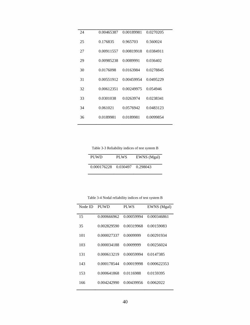
Table 3-3 Reliability indices of test system B

PUWD PLWS EWNS (Mgal)

0.000176228 0.030497 0.298043

Table 3-4 Nodal reliability indices of test system B

Node ID PUWD PLWS EWNS (Mgal)

15 0.000666962 0.00059994 0.000346861

35 0.002829590 0.00319968 0.00159083

101 0.000027337 0.0009999 0.00291934

103 0.000034188 0.0009999 0.00256024

131 0.000613219 0.00059994 0.0147385

143 0.000178544 0.00019998 0.000622353

153 0.000641868 0.0116988 0.0159395

166 0.004242990 0.00439956 0.0062022

41

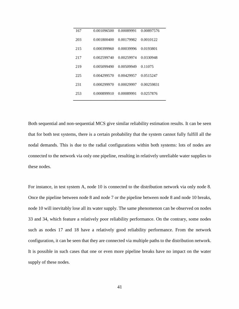
167 0.001096500 0.00089991 0.00897576

203 0.001800400 0.00179982 0.0010122

215 0.000399960 0.00039996 0.0193801

217 0.002599740 0.00259974 0.0330948

219 0.005099490 0.00509949 0.11075

225 0.004299570 0.00429957 0.0515247

231 0.000299970 0.00029997 0.00259831

253 0.000899910 0.00089991 0.0257876

Both sequential and non-sequential MCS give similar reliability estimation results. It can be seen

that for both test systems, there is a certain probability that the system cannot fully fulfill all the

nodal demands. This is due to the radial configurations within both systems: lots of nodes are

connected to the network via only one pipeline, resulting in relatively unreliable water supplies to

these nodes.

For instance, in test system A, node 10 is connected to the distribution network via only node 8.

Once the pipeline between node 8 and node 7 or the pipeline between node 8 and node 10 breaks,

node 10 will inevitably lose all its water supply. The same phenomenon can be observed on nodes

33 and 34, which feature a relatively poor reliability performance. On the contrary, some nodes

such as nodes 17 and 18 have a relatively good reliability performance. From the network

configuration, it can be seen that they are connected via multiple paths to the distribution network.

It is possible in such cases that one or even more pipeline breaks have no impact on the water

supply of these nodes.

42

Similarly, in test system B, while most of the other nodes are connected in a complex form, node

219 connects to the network via only node 217. This vulnerable connection has also made the

reliability performance of node 219 the worst among all the nodes in test system B. For the same

reason, it can also be seen that the reliability performances of nodes 225 and 217 are relatively

poor in test system B.

From the above analysis, it can be summarized that a radial network usually provides poor nodal

reliability performance. If no other factors are taken into consideration, from the design viewpoint

of a water distribution system, a single node needs to be connected to the main network via multiple

pipelines in order to achieve an improved reliability performance.

3.5 Conclusions

In this chapter a probabilistic methodology for performing quantitative reliability evaluation of

drinking water distribution systems considering both mechanical failures and hydraulic failures is

proposed. With the developed simulation software, case studies of reliability evaluation are

conducted on two test systems so as to illustrate the effectiveness of the proposed method.

For possible future work, the reliability model of individual components in the system can be

improved. In the real world, the functionalities of various components are affected by various

factors such as pipeline roughness and valve on/off statuses. In order to obtain a better estimation

of the reliability performance of the system, such factors need to be taken into consideration

comprehensively. The piped water quality could also be incorporated to define a set of more

comprehensive reliability indicators of the contemporary drinking water system.

43

Discussions, Conclusions and Future Work

In the previous chapters, reliability analysis of electrical power system and water distribution

system demonstrates some degree of similarities between these two interconnected, capacitated

systems. At the same time. differences in the reliability analysis also arise due to their own specific

characteristics. In this chapter findings obtained from conducting reliability analysis in both

electrical power system and water distribution system will be discussed and briefly compared, then

conclusion and future work of this thesis will be presented.

4.1 Similarities between Reliability Analysis of the Electrical Power System and the

Water Distribution System

The reason of the effectiveness of probabilistic reliability analysis method for both systems first

lies on the stochastic nature and similar modeling manner of the reliability characteristics of their

components. In electric power system, as discussed in [42], the reliability characteristic of each

component in the system can be modeled by a two-state representation. Probability for the

component to be in either status can be calculated, and a chronological historical operating

sequence (as used in sequential MCS method) can also be generated. In water distribution systems,

reliability modeling of components such as pipelines is performed in a similar manner. For instance,

the probability of failure can be determined by the time of repairing the pipe [51]. These similar

modeling techniques lead to the similar probabilistic reliability analysis procedures as well as the

similar statistical reliability metrics.

Reliability analysis of both systems share quite a few similarities. Since both the electric power

system and water distribution system are required to supply the customers with not only the

44

sufficient quantity but also the demanded quality, reliability analysis is in fact a multi-dimensional

problem. Apparently it is more difficult to evaluate the quality since it involves more factors. As

mentioned in [30], the quantification of the quality variation of a water distribution system is still

a complicated issue. And currently in the field of water distribution system reliability most studies

are mainly focused on the reliability concept raised in [52], which defines the acceptable water

supply as the water pressure being higher than or equal to the demanded nodal pressure. In the

power systems field, for electric utilities it is important to supply electricity to customers with both

satisfactory quality and reliability [53]. Power quality related issues remain an active research field

in a smart grid environment [54].

4.2 Differences between Reliability Analysis of Electric Power System and Water

Distribution System

The differences between electric power system and water distribution system are mainly due to

their specific physical properties and operating conditions. Although the components in these

systems can be modeled in a similar fashion, in practice these components are very different from

each other. For example, roughness for the pipelines in water distribution systems and resistances

for transmission lines in electrical power systems are comparable properties. However, in reality

they have completely different definitions, and in the reliability analysis they are also treated

differently. Resistances of transmission lines are conventionally considered as static values in the

reliability evaluation process, but in lots of the studies about water distribution system reliability,

pipeline roughness is considered as an important random variable to better characterize the

probabilistic hydraulic behaviors of the system.

45

Other differences may be more at the system level. Differences in terms of operating strategies

and network topologies could lead to different reliability performances in these systems.

Furthermore, due to the fact that electric energy cannot be stored for a long time at a large scale

and the nature of dynamics of electric power system, a number of electric quantities change very

rapidly. Therefore, it has become very important to analyze the system behavior in the transient

process. In the power system reliability field, the concept of system security is used to evaluate the

ability of the system to respond to the disturbances during these transient processes [8]. Yet things

are different in water distribution systems. Changes of nodal pressures are not as fast as changes

of electrical quantities in the electric power system. In addition, water can be stored in facilities

such as tanks and water towers for a long time.

4.3 Conclusions and Future Work

In this thesis, probabilistic reliability analysis of electric power system incorporating smart grid

technologies and water distribution system are first introduced and discussed. Then, system

reliabilities are modeled and investigated in detail. Finally, the proposed models and methods are

validated by simulation studies with a discussion on their similarities and differences.

Smart grid technologies such as DTR and OTS are becoming more and more practical nowadays,

which are believed to be viable operating strategies in a smart grid environment. In this thesis,

these two technologies are incorporated into the traditional reliability analysis procedure of electric

power systems. Simulation results have shown that by incorporating these technologies the

reliability of the overall power system can be enhanced. And the proposed methodology is also

validated via extensive simulation studies.

46

As one of the nation’s critical infrastructures, reliability performance of the water distribution

system has always been highly concerned. In this thesis, a probabilistic reliability analysis method

using Monte Carlo simulation is proposed. Case studies are performed to give the estimation of

the overall reliability of two test water systems, and also to illustrate the effectiveness of the

proposed method.

Although in this thesis the probabilistic reliability analysis method has been successfully applied

in the electric power system and the water distribution system, what this thesis presents is by no

means the final answer or the best solution to the reliability analysis in these fields. There is still

room for further extending the proposed models and algorithms. With a deep understanding of

reliability modeling at both component and system levels in other domains, the models and

methods developed in this thesis are also promising to be extended to other engineering fields.

47

References

[1] B. Liscouski and W. Elliot, "Final report on the august 14, 2003 blackout in the united

states and canada: Causes and recommendations," A report to US Department of Energy,

vol. 40, 2004.

[2] P. L. Anderson and I. K. Geckil, "Northeast blackout likely to reduce US earnings by $6.4

billion," Anderson Economic Group, 2003.

[3] S. Denyer and R. Lakshmi, "India blackout, on second day, leaves 600 million without

power," The Washington Post, 2012.

[4] H. Pidd, "India blackouts leave 700 million without power," The guardian, vol. 31, 2012.

[5] S. E. Hrudey, "Waterborne outbreak of cryptosporidiosis in North Battleford, Canada,"

Case Studies in Environmental Engineering and Science. Available via DIALOG.

http://www.aeespfoundation. org/publications/pdf/AEESP_CS_2. pdf, 2006.

[6] M. S. Islam, R. Sadiq, M. J. Rodriguez, H. Najjaran, A. Francisque, and M. Hoorfar, "Water

distribution system failure: a framework for forensic analysis," Environment Systems and

Decisions, vol. 34, pp. 168-179, 2014.

[7] M. Hanna-Attisha, J. LaChance, R. C. Sadler, and A. Champney Schnepp, "Elevated blood

lead levels in children associated with the Flint drinking water crisis: a spatial analysis of

risk and public health response," American journal of public health, vol. 106, pp. 283-290,

2016.

[8] R. Allan, Reliability evaluation of power systems: Springer Science & Business Media,

2013.

[9] J. M. Wagner, U. Shamir, and D. H. Marks, "Water distribution reliability: analytical

methods," Journal of Water Resources Planning and Management, vol. 114, pp. 253-275,

1988.

[10] M. J. Cullinane, K. E. Lansey, and L. W. Mays, "Optimization-availability-based design

of water-distribution networks," Journal of Hydraulic Engineering, vol. 118, pp. 420-441,

1992.

[11] B. Zhuang, K. Lansey, and D. Kang, "Resilience/availability analysis of municipal water

distribution system incorporating adaptive pump operation," Journal of Hydraulic

Engineering, vol. 139, pp. 527-537, 2012.

48

[12] E. B. Fisher, R. P. Neill, and M. C. Ferris, "Optimal transmission switching," Power

Systems, IEEE Transactions on, vol. 23, pp. 1346-1355, 2008.

[13] J. Ausen, B. F. Fitzgerald, E. A. Gust, D. C. Lawry, J. P. Lazar, and R. L. Oye, "Dynamic

thermal rating system relieves transmission constraint," in Transmission & Distribution

Construction, Operation and Live-Line Maintenance, 2006. ESMO 2006. IEEE 11th

International Conference on, 2006.

[14] B. Gorenstin, L. Terry, M. Pereira, and L. Pinto, "Integrated network topology optimization

and generation rescheduling for power system security applications," in IASTED Intl.

Symposium—High Tech. in the Power Industry, 1986, pp. 110-114.

[15] D. M. Greenwood, J. P. Gentle, K. S. Myers, P. J. Davison, I. J. West, J. W. Bush, et al.,

"A comparison of real-time thermal rating systems in the US and the UK," Power Delivery,

IEEE Transactions on, vol. 29, pp. 1849-1858, 2014.

[16] C. J. Wallnerstrom, Y. Huang, and L. Soder, "Impact from Dynamic Line Rating on Wind

Power Integration," Smart Grid, IEEE Transactions on, vol. 6, pp. 343-350, 2015.

[17] J. Teh and I. Cotton, "Reliability Impact of Dynamic Thermal Rating System in Wind

Power Integrated Network," IEEE Transactions on Reliability, vol. 65, pp. 1081-1089,

2016.

[18] W. J. Steeley, B. L. Norris, and A. K. Deb, "Ambient temperature corrected dynamic

transmission line ratings at two PG&E locations," IEEE Transactions on Power

Delivery, vol. 6, pp. 1234-1242, 1991.

[19] J. Engelhardt and S. Basu, "Design, installation, and field experience with an overhead

transmission dynamic line rating system," in Transmission and Distribution Conference,

1996. Proceedings., 1996 IEEE, 1996, pp. 366-370.

[20] S. D. Foss, S. H. Lin, and R. A. Fernandes, "Dynamic thermal line ratings part I dynamic

ampacity rating algorithm," IEEE Transactions on Power Apparatus and Systems, pp.

1858-1864, 1983.

[21] S. D. Foss, S. H. Lin, H. R. Stillwell, and R. A. Fernandes, "Dynamic Thermal Line Ratings

Part II Conductor Temperature Sensor and Laboratory Field test Evaluation," IEEE

Transactions on Power Apparatus and Systems, pp. 1865-1876, 1983.

[22] S. Jupe, D. Kadar, G. Murphy, M. Bartlett, and K. Jackson, "Application of a dynamic

thermal rating system to a 132kV distribution network," in Innovative Smart Grid

Technologies (ISGT Europe), 2011 2nd IEEE PES International Conference and

Exhibition on, 2011, pp. 1-8.

49

[23] A. Safdarian, M. Z. Degefa, M. Fotuhi-Firuzabad, and M. Lehtonen, "Benefits of real-time

monitoring to distribution systems: Dynamic thermal rating," Smart Grid, IEEE

Transactions on, vol. 6, pp. 2023-2031, 2015.

[24] R. P. O'Neill, R. Baldick, U. Helman, M. H. Rothkopf, and W. Stewart Jr, "Dispatchable

transmission in RTO markets," IEEE Transactions on Power Systems, vol. 20, pp. 171-179,

2005.

[25] G. Schnyder and H. Glavitsch, "Security enhancement using an optimal switching power

flow," Power Systems, IEEE Transactions on, vol. 5, pp. 674-681, 1990.

[26] K. W. Hedman, R. P. O'Neill, E. B. Fisher, and S. S. Oren, "Optimal transmission switching

with contingency analysis," Power Systems, IEEE Transactions on, vol. 24, pp. 1577-1586,

2009.

[27] C. Zhang and J. Wang, "Optimal transmission switching considering probabilistic

reliability," Power Systems, IEEE Transactions on, vol. 29, pp. 974-975, 2014.

[28] S. Diop, P. M'mayi, D. Lisbjerg, and R. Johnstone, Vital water graphics: an overview of

the state of the world's fresh and marine waters vol. 1: UNEP/Earthprint, 2002.

[29] Y. Bao and L. W. Mays, "Model for water distribution system reliability," Journal of

Hydraulic Engineering, vol. 116, pp. 1119-1137, 1990.

[30] C. Xu and I. C. Goulter, "Probabilistic model for water distribution reliability," Journal of

Water Resources Planning and Management, vol. 124, pp. 218-228, 1998.

[31] D. Wood, "KYPipe reference manual," University of Kentucky, 1995.

[32] L. A. Rossman, "The epanet programmer’s toolkit for analysis of water distribution

systems," in Annual Water Resources Planning and Management Conference, 1999, p.

10.7.

[33] S.-J. Wu, J.-H. Yoon, and R. G. Quimpo, "Capacity-weighted water distribution system

reliability," Reliability Engineering & System Safety, vol. 42, pp. 39-46, 1993.

[34] R. Gupta and P. R. Bhave, "Reliability analysis of water-distribution systems," Journal of

Environmental Engineering, vol. 120, pp. 447-461, 1994.

[35] D. Khomsi, G. Walters, A. Thorley, and D. Ouazar, "Reliability tester for water-

distribution networks," Journal of Computing in Civil Engineering, vol. 10, pp. 10-19,

1996.

50

[36] N. Duan, L. W. Mays, and K. E. Lansey, "Optimal reliability-based design of pumping and

distribution systems," Journal of Hydraulic Engineering, vol. 116, pp. 249-268, 1990.

[37] D. Li, T. Dolezal, and Y. Y. Haimes, "Capacity reliability of water distribution networks,"

Reliability Engineering & System Safety, vol. 42, pp. 29-38, 1993.

[38] F. Bouchart and I. Goulter, "Reliability improvements in design of water distribution

networks recognizing valve location," Water Resources Research, vol. 27, pp. 3029-3040,

1991.

[39] "IEEE Standard for Calculating the Current-Temperature Relationship of Bare Overhead

Conductors Institute of Electrical and Electronics Engineers standard# 738, 1993,

Calculation Module 23," Institute of Electrical and Electronics Engineers standard# 738,

1993.

[40] W. CIGRE, "The thermal behavior of overhead conductors," Electra, pp. 107-125, Oct.

1992.

[41] S. Binato, M. V. F. Pereira, and S. Granville, "A new Benders decomposition approach to

solve power transmission network design problems," IEEE Transactions on Power Systems,

vol. 16, pp. 235-240, 2001.

[42] W. Li, Reliability assessment of electric power systems using Monte Carlo methods:

Springer Science & Business Media, 2013.

[43] P. M. Subcommittee, "IEEE reliability test system," Power Apparatus and Systems, IEEE

Transactions on, pp. 2047-2054, 1979.

[44] C. Grigg, P. Wong, P. Albrecht, R. Allan, M. Bhavaraju, R. Billinton, et al., "The IEEE

reliability test system-1996. A report prepared by the reliability test system task force of

the application of probability methods subcommittee," IEEE Transactions on power

systems, vol. 14, pp. 1010-1020, 1999.

[45] (Mar. 6, 2016). Normals Hourly, Milwaukee, WI (hourly). Available:

https://www.ncdc.noaa.gov/cdo-web/datasets

[46] "IEEE Standard for Calculating the Current-Temperature Relationship of Bare Overhead

Conductors," IEEE Std 738-2012 (Revision of IEEE Std 738-2006 - Incorporates IEEE Std

738-2012 Cor 1-2013), pp. 1-72, 2013.

[47] R. Billinton and R. N. Allan, Reliability evaluation of engineering systems: Springer, 1992.

51

[48] J. M. Wagner, U. Shamir, and D. H. Marks, "Water distribution reliability: simulation

methods," Journal of Water Resources Planning and Management, vol. 114, pp. 276-294,

1988.

[49] A. Ostfeld, D. Kogan, and U. Shamir, "Reliability simulation of water distribution

systems–single and multiquality," Urban Water, vol. 4, pp. 53-61, 2002.

[50] L. A. Rossman, "EPANET 2: users manual," 2000.

[51] I. C. Goulter and A. Coals, "Quantitative approaches to reliability assessment in pipe

networks," Journal of Transportation Engineering, vol. 112, pp. 287-301, 1986.

[52] C. Xu and I. C. Goulter, "Reliability-based optimal design of water distribution networks,"

Journal of Water Resources Planning and Management, vol. 125, pp. 352-362, 1999.

[53] M. H. Bollen, Understanding power quality problems vol. 3: IEEE press New York, 2000.

[54] A. T. O. RELIABILITY, "Measurement practices for reliability and power quality," 2004.

Documents

Probabilistic Reliability Analysis of Electric Power