Probabilistic D-Clustering - Ben-Israel.netbenisrael.net/J-CLASSIFICATION-07.pdf · The probabilistic d–clustering algorithm is presented in Section 4. It is a generalization, to

Journal of Classification 25 (2007)DOI: 10.1007/s00357-007-0021-y

Probabilistic D-Clustering

Adi Ben-Israel

Rutgers University, New Jersey

Cem Iyigun

Rutgers University, New Jersey

Abstract: We present a new iterative method for probabilistic clustering of data.Given clusters, their centers and the distances of data points from these centers, theprobability of cluster membership at any point is assumed inversely proportional tothe distance from (the center of) the cluster in question. This assumption is our work-ing principle.

The method is a generalization, to several centers, of the Weiszfeld method forsolving the Fermat–Weber location problem. At each iteration, the distances (Euclid-ean, Mahalanobis, etc.) from the cluster centers are computed for all data points, andthe centers are updated as convex combinations of these points, with weights deter-mined by the above principle. Computations stop when the centers stop moving.

Progress is monitored by the joint distance function a measure of distance fromall cluster centers, that evolves during the iterations, and captures the data in its lowcontours.

The method is simple, fast (requiring a small number of cheap iterations) andinsensitive to outliers.

Keywords: Clustering; Probabilistic clustering; Mahalanobis distance; Harmonicmean; Joint distance function; Weiszfeld method; Similarity matrix.

Authors’ Address: RUTCOR–Rutgers Center for Operations Research, RutgersUniversity, 640 Bartholomew Rd., Piscataway, NJ 08854-8003, USA, e-mail: adi.benisrael@gmail. com, [email protected]

A. Ben-Israel and C. Iyigun

1. Introduction

A cluster is a set of data points that are similar, in some sense, andclustering is a process of partitioning a data set into disjoint clusters.

Clustering is a basic tool in statistics and machine learning, and hasbeen applied in pattern recognition, medical diagnostics, data mining, biol-ogy, finance and other areas.

We take data points to be vectors x = (x1, . . . , xn) ∈ Rn, and inter-

pret “similar” as “close”, in terms of a distance function d(x,y) in Rn, such

asd(x,y) = ‖x − y‖, ∀x,y ∈ R

n, (1)

where the norm ‖ · ‖ is elliptic, defined for u = (ui) by

‖u‖ = 〈u, Qu〉1/2, (2)

with 〈·, ·〉 the standard inner product, and Q a positive definite matrix. Inparticular, Q = I gives the Euclidean norm,

‖u‖ = 〈u,u〉1/2, (3)

and the Mahalanobis distance corresponds to Q = Σ−1, where Σ is thecovariance matrix of the data involved.

Example 1. A data set in R2 with N = 200 data points is shown in Figure 1.

The data was simulated, from normal distributions N(µi, Σi), with:

µ1 = (0, 0), Σ1 =(

0.1 00 1

), (100 points) ,

µ2 = (3, 0), Σ2 =(

1 00 0.1

), (100 points) .

This data will serve to illustrate Examples 2–5 below.

The clustering problem is, given a dataset D consisting of N datapoints

{x1, x2, . . . ,xN} ⊂ Rn,

and an integer K, 1<K <N , to partition D into K clusters C1, . . . , CK .Data points are assigned to clusters using a clustering criterion. In

distance clustering, abbreviated d–clustering, the clustering criterion is met-ric: With each cluster Ck we associate a center ck, for example its centroid,and each data point is assigned to the cluster to whose center it is the near-est. After each such assignment, the cluster centers may change, resulting in


−1 0 1 2 3 4 5

−2.5

−2

−1.5

−1

−0.5

0

0.5

1

1.5

2

2.5

Figure 1. A data set in R2

re–assignments. Such an algorithm will therefore iterate between updatingthe centers and re–assignments.

A commonly used clustering criterion is the sum–of–squares of Euclid-ean distances,

K∑k=1

∑xi∈Ck

‖ xi − ck ‖2, (4)

to be minimized by the sought clusters C1, . . . , CK . The well known k–means clustering algorithm [5] uses this criterion.

In probabilistic clustering the assignment of points to clusters is “soft”,in the sense that the membership of a data point x in a cluster Ck is given as aprobability, denoted by pk(x). These are subjective probabilities, indicatingstrength of belief in the event in question.

Let a distance functiondk( · , · ) (5)

be defined for each cluster Ck. These distance functions are, in general,different from one cluster to another. For each data point x ∈ D, we thencompute:

• the distance dk(x, ck), also denoted by dk(x) (since dk is used only fordistances from ck), or just dk if x is understood, and

• a probability that x is a member of Ck, denoted by pk(x), or just pk.

Various relations between probabilities and distances can be assumed,resulting in different ways of clustering the data. In our experience, the fol-lowing assumption has proved useful: For any point x, and all k = 1, · · · , K

pk(x) dk(x) = constant, depending on x .


This model is our working principle in what follows, and the basis ofthe probabilistic d–clustering approach of Section 2.

The above principle owes its versatility to the different ways of choos-ing the distances dk(·). It is also natural to consider increasing functions ofsuch distances, and one useful choice is

pk(x)edk(x) = constant, depending on x ,

giving the probabilistic exponential d–clustering approach of Section 3.The probabilistic d–clustering algorithm is presented in Section 4. It

is a generalization, to several centers, of the Weizsfeld method for solv-ing the Fermat–Weber location problem, see Section 2.5, and convergencefollows as in [15]. The updates of the centers use an extremal principle,described in Section 2.3. The progress of the algorithm is monitored by thejoint distance function, a distance function that captures the data in its lowcontours, see Section 2.2. The centers updated by the algorithm are station-ary points of the joint distance function.

The paper concludes with a small example, Section 5, analyzing theliberal–conservative divide of the U.S. Supreme Court.

For other approaches to probabilistic clustering see the surveys in [7],[18], and the seminal article [19] unifying clustering methods in the frame-work of modern optimization theory.

2. Probabilistic D–Clustering

There are several ways to model the relationship between distancesand probabilities. The simplest model, and our working principle (or ax-iom), is the following:

Principle 1. For each x ∈ D, and each cluster Ck,

pk(x) dk(x) = constant, depending on x . (6)

Cluster membership is thus more probable the closer the data pointis to the cluster center. Note that the constant in (6) is independent of thecluster k.

2.1 Probabilities

From Principle 1, and the fact that probabilities add to one, we get

Theorem 1. Let the cluster centers {c1, c2, . . . , cK} be given, let x be adata point, and let {dk(x) : k = 1, . . . , K} be its distances from the givencenters. Then the membership probabilities of x are


pk(x) =

∏j �=k

dj(x)

K∑t=1

∏j �=t

dj(x), k = 1, . . . , K. (7)

Proof. Using (6) we write for t, k

pt(x) =(

pk(x)dk(x)dt(x)

).

SinceK∑

t=1pt(x) = 1,

pk(x)K∑

t=1

(dk(x)dt(x)

)= 1.

∴ pk(x) =1

K∑t=1

(dk(x)dt(x)

) =

∏j �=k

dj(x)

K∑t=1

∏j �=t

dj(x).

�

In particular, for K=2,

p1(x) =d2(x)

d1(x) + d2(x), p2(x) =

d1(x)d1(x) + d2(x)

, (8)

and for K = 3,

p1(x) =d2(x)d3(x)

d1(x)d2(x) + d1(x)d3(x) + d2(x)d3(x), etc. (9)

Note: See [6] for related work in a different context. In particular, ourequation (8) is closely related to [6, Eq. (5)].

2.2 The Joint Distance Function

We denote the constant in (6) by D(x), a function of x. Then

pk(x) =D(x)dk(x)

, k = 1, . . . , K.


Since the probabilities add to one we get,

D(x) =

K∏k=1

dk(x, ck)

K∑t=1

∏j �=t

dj(x, cj). (10)

The function D(x), called the joint distance function (abbreviatedJDF) of x, has the dimension of distance, and measures the distance ofx from all cluster centers. Here are special cases of (10), for K = 2,

D(x) =d1(x) d2(x)

d1(x) + d2(x), (11)

and for K = 3,

D(x) =d1(x) d2(x) d3(x)

d1(x) d2(x) + d1(x) d3(x) + d2(x) d3(x). (12)

The JDF of the whole data set D is the sum of (10) over all points,and is a function of the K cluster centers, say,

F (c1, c2, · · · , cK) =N∑

i=1

K∏k=1

dk(xi, ck)

K∑t=1

∏j �=t

dj(xi, cj). (13)

Example 2. Figure 2 shows level sets of the JDF (11), with Mahalanobisdistances

dk(x, ck) =√

(x − ck)T Σ−1k (x − ck) , (14)

c1 = µ1, c2 = µ2, and Σ1, Σ2 as in Example 1.

Notes:(a) The JDF D(x) of (10) is a measure of the classifiability of the point x inquestion. It is zero if and only if x coincides with one of the cluster centers,in which case x belongs to that cluster with probability 1. If all the distancesdk(x, ck) are equal, say equal to d, then D(x) = d/k and all pk(x) = 1/K,showing indifference between the clusters. As the distances dk(x) increase,so does D(x), indicating greater uncertainty about the cluster where x be-longs.(b) The JDF (10) is, up to a constant, the harmonic mean of the distancesinvolved, see [1] for an elucidation of the role of the harmonic mean in con-tour approximation of data. A related concept in ecology is the home range,shown in [4] to be the harmonic mean of the area moments in question.


−3 −2 −1 0 1 2 3 4 5−5

−4

−3

−2

−1

0

1

2

3

4

5

0.73881

0.73

881

1.47761.4776

1.4

776

1.47

76

1.4776

2.2164

2.2164

2.21

64

2.2164

2.21

64

2.2164

2.9552

2.9552

2.9552

2.95

52

2.9552 2.95

52

2.9552

3.69

41

3.6941

3.6941

3.6941

3.6941

3.6941

3.69

41

3.6941

4.43

29

4.4329

4.4329

4.4329

4.43

29

4.4329

5.17

17

5.1717

5.1717

5.1717

5.17

17

5.1717

5.9105

5.9105

6.6493

6.6493

Figure 2. Level sets of a joint distance function

2.3 An Extremal Principle

For simplicity consider the case of two clusters (the results are easilyextended to the general case.)

Let x be a given data point with distances d1(x), d2(x) to the clustercenters. Then the probabilities in (8) are the optimal solutions p1, p2 of theextremal problem

Minimize d1(x) p21 + d2(x) p2

2 (15)

subject to p1 + p2 = 1p1, p2 ≥ 0

Indeed, the Lagrangian of this problem is

L(p1, p2, λ) = d1(x) p21 + d2(x) p2

2 − λ(p1 + p2 − 1) (16)

and setting the partial derivatives (with respect to p1, p2) equal to zero givesthe principle (6),

p1 d1(x) = p2 d2(x) .

Substituting the probabilities (8) in the Lagrangian (16) we get theoptimal value of (15),

L∗(p1(x), p2(x), λ) =d1(x) d2(x)

d1(x) + d2(x), (17)

which is the JDF (11) again.


The extremal problem for a data set D = {x1, x2, . . . , xN} ⊂ Rn

is, accordingly,

MinimizeN∑

i=1

(d1(xi) p1(xi)2 + d2(xi) p2(xi)2

)(18)

subject to p1(xi) + p2(xi) = 1,

p1(xi), p2(xi) ≥ 0, i = 1, . . . , N.

This problem separates into N problems like (15), and its optimal value is

N∑i=1

d1(xi) d2(xi)d1(xi) + d2(xi)

(19)

the JDF (13) of the data set, with K = 2.

Note: The explanation for the strange appearance of “probabilities squared”above, is that (15) is a smoothed version of the “real” clustering problem,namely,

min {d1, d2},which is nonsmooth, see [19] for a unified development of smoothed clus-tering methods.

2.4 Centers

We write (18) as a function of the cluster centers c1, c2,

f(c1, c2) =N∑

i=1

(d1(xi, c1) p1(xi)2 + d2(xi, c2) p2(xi)2

). (20)

If a point xi coincides with a center, say xi = c1, then d1(xi) =0, p1(xi) = 1 and p2(xi) = 0. This point contributes zero to the summation.

For the special case of Euclidean distances, the minimizers of (20)assume a simple form as convex combinations of the data points.

Theorem 2. Let the distance functions d1, d2 in (20) be Euclidean,

dk(x, ck) = ‖x − ck‖ , k = 1, 2 , (21)

so that

f(c1, c2) =∑

i=1,...,N

(‖xi − c1‖ p1(xi)2 + ‖xi − c2‖ p2(xi)2)

, (22)


and let the probabilities be given for i = 1, . . . , N . We make the followingassumption about the minimizers c1, c2 of (22):

c1, c2 do not coincide with any of the points xi, i = 1, . . . , N . (23)

Then the minimizers c1, c2 are given by

ck =∑

i=1,...,N

⎛⎜⎝ uk(xi)∑

j=1,...,N

uk(xj)

⎞⎟⎠xi , (24)

where

uk(xi) =pk(xi)2

dk(xi, ck), (25)

for k = 1, 2, or equivalently, using (8),

u1(xi) =d2(xi, c2)2

d1(xi, c1) (d1(xi, c1) + d2(xi, c2))2,

u2(xi) =d1(xi, c1)2

d2(xi, c2) (d1(xi, c1) + d2(xi, c2))2. (26)

Proof. The gradient of d(x, c) = ‖x − c‖ with respect to c is, for x �= c,

∇c ‖x − c‖ = − x − c‖x − c‖ = − x − c

d(x, c). (27)

By Assumption (23), the gradient of (22) with respect to ck is

∇ckf(c1, c2) = −

∑i=1,...,N

xi − ck

‖xi − ck‖ pk(xi)2

= −∑

i=1,...,N

xi − ck

dk(xi, ck)pk(xi)2 , k = 1, 2 .

(28)

Setting the gradient equal to zero, and summing like terms, we get

∑i=1,...,N

(pk(xi)2

dk(xi, ck)

)xi =

⎛⎝ ∑

i=1,...,N

pk(xi)2

dk(xi, ck)

⎞⎠ ck , (29)

proving (24)–(26).

�

The same formulas for the centers c1, c2 hold if the norm used in (22)is elliptic.


Corollary 1. Let the distance functions d1, d2 in (20) be elliptic,

dk(x, ck) = 〈(x − ck), Qk(x − ck)〉1/2 , (30)

with positive–definite matrices Qk. Then the minimizers c1, c2 of (20) aregiven by (24)–(26).

Proof. The gradient of d(x, c) = 〈(x − c), Q(x − c)〉1/2 with respect to cis, for x �= c,

∇c d(x, c) = −Q(x − c)d(x, c)

.

Therefore the analog of (28) is

∇ckf(c1, c2) = −Qk

∑i=1,...,N

xi − ck

dk(xi, ck)pk(xi)2 , (31)

and since Qk is nonsingular, it can be “cancelled” when we set the gradientequal to zero. The rest of the proof is as in Theorem 2.�

Corollary 1 applies, in particular, to the Mahalanobis distance (14)

dk(x, ck) =√

(x − ck)T Σ−1k (x − ck) ,

where Σk is the covariance matrix of the cluster Ck.The formulas (24)–(25) are also valid in the general case of K clus-

ters, where the analog of (20) is

f(c1, c2, · · · , cK) =∑

i=1,...,N

K∑k=1

dk(xi, ck) pk(xi)2 . (32)

Corollary 2. Let the distance functions dk in (32) be elliptic, as in (30), andlet the probabilities pk(xi) be given. Then the minimizers c1, c2, · · · , cK of(32) are given by (24)–(25) for k = 1, 2, · · · , K.

Proof. The proof of Corollary 1 holds in the general case, since the mini-mizers are calculated separately.�

2.5 The Weiszfeld Method

In the case of one cluster (where the probabilities are all 1 and there-fore of no interest) the center formulas (24)–(25) reduce to

c =∑

i=1,...,N

⎛⎜⎝ 1/d(xi, c)∑

j=1,...,N

1/d(xj , c)

⎞⎟⎠xi , (33)


giving the minimizer of f(c) =N∑

i=1d(xi, c). Formula (33) can be used

iteratively to update the center c (on the left) as a convex combination ofthe points xi with weights depending on the current center. This iteration isthe Weiszfeld method [20] for solving the Fermat–Weber location problem,see [20], [16]. Convergence of Weiszfeld’s method was established in Kuhn[15] by modifying the gradient ∇f(c) so that it is always defined, see [17]for further details. However, the modification is not carried out in practicesince, as shown by Kuhn, the set of initial points c for which it ever becomesnecessary is denumerable.

In what follows we use the formulas (24)–(25) iteratively to updatethe centers. Convergence can be proved by adapting the arguments of Kuhn[15], but as there it requires no special steps in practice.

2.6 The Centers and the Joint Distance Function

The centers given by (24)–(25) are related to the JDF (13) of the dataset. Consider first the case of K = 2 clusters, where (13) reduces to

F (c1, c2) =N∑

i=1

d1(xi, c1) d2(xi, c2)d1(xi, c1) + d2(xi, c2)

. (34)

The points ck where ∇ckF (c1, c2) = 0, k = 1, 2, are called stationary

points of (34).

Theorem 3. Let the distances d1, d2 in (34) be elliptic, as in (30). Then thestationary points of F (c1, c2) are given by (24)–(26).

Proof. Let the distances dk be Euclidean, dk(x) = ‖x− ck‖. It is enough toprove the theorem for one center, say c1. Using (27) we derive

∇c1 F (c1, c2) =

N∑i=1

(d1(xi) + d2(xi)) d2(xi)(−xi − c1

d1(xi)

)+ d1(xi) d2(xi)

(xi − c1

d1(xi)

)(d1(xi) + d2(xi))2

=N∑

i=1

−d2(xi)2 (xi − c1)d1(xi) (d1(xi) + d2(xi))2

. (35)


Setting (35) equal to zero, and summing like terms, we get⎛⎝ N∑

j=1

d2(xj)2

d1(xj) (d1(xj) + d2(xj))2

⎞⎠ c1 =

N∑i=1

(d2(xi)2

d1(xi) (d1(xi) + d2(xi))2

)xi ,

duplicating (24)–(26). If the distances are elliptic, as in (30), then the analogof (35) is,

∇c1 F (c1, c2) =N∑

i=1

−d2(xi)2 Q1 (xi − c1)d1(xi) (d1(xi) + d2(xi))2

and since Q1 is nonsingular, it can be “cancelled” when the gradient is setequal to zero.�

In the above proof the stationary points c1, c2 are calculated sepa-rately, and the calculation does not depend on there being 2 clusters. Wethus have:

Corollary 3. Consider a data set with K clusters, and elliptic distancesdk. Then the stationary points of the JDF (13) are the centers ck given by(24)–(25).

Note: The JDF (10) is zero exactly at the K centers {ck}, and is positiveelsewhere. These centers are therefore the global minimizers of (10). How-ever, the function (10) is not convex, not even quasi–convex, and may haveother stationary points, that are necessarily saddle points.

2.7 Why d and Not d2?

The extremal principle (18), which is the basis of our work, is linearin the distances dk,

Minimize∑

k

dk p2k.

We refer to this as the d–model.In clustering, and statistics in general, it is customary to use the dis-

tances squared in the objective function,

Minimize∑

k

d2k.

We call this the d2–model.


The d2–model has a long tradition, dating back to Gauss, and is en-dowed with a rich statistical theory. There are geometrical advantages (Pytha-goras Theorem), as well as analytical (linear derivatives).

The d–model is suggested by the analogy between clustering and lo-cation problems, where sums of distances (not distances squared) are mini-mized. Our center formulas (24)–(25) are thus generalizations of the Weisz-feld Method to several facilities, see Section 2.5.

An advantage of the d–model is its robustness. Indeed the formula(25), which does not follow from the d2–model, guarantees that outliers willnot affect the center locations.

2.8 Other Principles

There are alternative ways of modelling the relations between dis-tances and probabilities. For example:

Principle 2. For each x ∈ D, and each cluster Ck, the probability pk =pk(x) and distance dk = dk(x) are related by

pαk dβ

k = constant, depending on x . (36)

where the exponents α, β are positive.

For the case of 2 clusters we get, by analogy with (8) and (18) respec-tively, the probabilities

p1(x) =d2(x)β/α

d1(x)β/α + d2(x)β/α, p2(x) =

d1(x)β/α

d1(x)β/α + d2(x)β/α, (37)

and an extremal principle,

MinimizeN∑

i=1

(d1(xi)β p1(i)α+1 + d2(xi)β p2(i)α+1

)(38)

subject to p1(i) + p2(i) = 1p1(i), p2(i) ≥ 0

where p1(i), p2(i) are the cluster probabilities at xi.The Fuzzy Clustering Method [2], [3], which is an extension of k-

means method, uses β = 2 and allows different choices of α. For α = 2, itgives the same probabilities as (7), however the center updates are differentthan (24)–(25).


3. Probabilistic Exponential D–Clustering

Any increasing function of the distance can be used in Principle 1.The following model, with probabilities decaying exponentially as distancesincrease, has proved useful in our experience.

Principle 3. For each x ∈ D, and each cluster Ck, the probability pk(x)and distance dk(x) are related by

pk(x) edk(x) = E(x), a constant depending on x . (39)

Most results of Section 2 hold also for Principle 3, with the distance dk(x)replaced by edk(x). Thus the analog of the probabilities (8) is

p1(x) =ed2(x)

ed1(x) + ed2(x), p2(x) =

ed1(x)

ed1(x) + ed2(x), (40)

or equivalently

p1(x) =e−d1(x)

e−d1(x) + e−d2(x), p2(x) =

e−d2(x)

e−d1(x) + e−d2(x). (41)

Similarly, since the probabilities add to 1, the constant in (39) is

E(x) =ed1(x)+d2(x)

ed1(x) + ed2(x), (42)

called the exponential JDF.

3.1 An Extremal Principle

The probabilities (40) are the optimal solutions of the problem

minp1,p2

{ed1p2

1 + ed2p22 : p1 + p2 = 1 , p1, p2 ≥ 0

}, (43)

whose optimal value, obtained by substituting the probabilities (40), is againthe exponential JDF (42).

The extremal problem for a data set D = {x1, x2, . . . , xN} ⊂ Rn,

partitioned into 2 clusters, is the following analog of (18)

MinimizeN∑

i=1

(ed1(xi) p1(i)2 + ed2(xi) p2(i)2

)(44)

subject to p1(i) + p2(i) = 1p1(i), p2(i) ≥ 0


where p1(i), p2(i) are the cluster probabilities at xi. The problem separatesinto N problems like (43), and its optimal value is

N∑i=1

ed1(xi)+d2(xi)

ed1(xi) + ed2(xi), (45)

the exponential JDF of the whole data set.Alternatively, (39) follows from the “smoothed” extremal principle

minp1,p2

{2∑

k=1

pk dk +2∑

k=1

pk log pk : p1 + p2 = 1 , p1, p2 ≥ 0

}, (46)

obtained by adding an entropy term to∑

pk dk. Indeed the Lagrangian of(46) is

L(p1, p2, λ) =2∑

k=1

pk dk +2∑

k=1

pk log pk − λ (p1 + p2 − 1) .

Differentiation with respect to pk, and equating to 0, gives

dk + 1 + log pk − λ = 0

which is (39).

3.2 Centers

We write (44) as a function of the cluster centers c1, c2,

f(c1, c2) =N∑

i=1

(ed1(xi,c1) p1(xi)2 + ed2(xi,c2) p2(xi)2

)(47)

and for elliptic distances we can verify, as in Theorem 2, that the minimizersof (47) are given by,

ck =N∑i=1

⎛⎜⎜⎜⎝ uk(xi)

N∑j=1

uk(xj)

⎞⎟⎟⎟⎠xi , (48)

where (compare with (25)),

uk(xi) =pk(xi)2 edk(xi)

dk(xi), (49)


or equivalently,

u1(xi) =e−d1(xi)/d1(xi)

(e−d1(xi) + e−d2(xi))2, u2(xi) =

e−d2(xi)/d2(xi)(e−d1(xi) + e−d2(xi))2

.

(50)

As in Theorem 3, these minimizers are the stationary points of the JDF,given here as

F (c1, c2) =N∑

i=1

ed1(xi,c1)+d2(xi,c2)

ed1(xi,c1) + ed2(xi,c2). (51)

Finally we can verify, as in Corollary 2, that the results hold in the generalcase of K clusters.

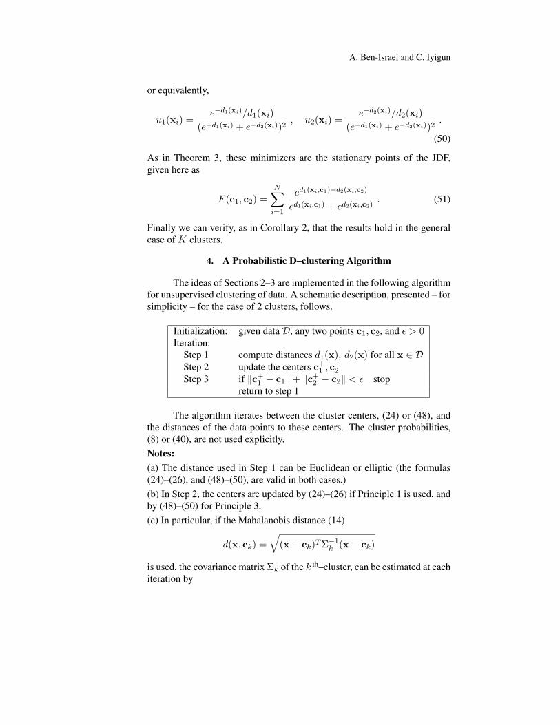
4. A Probabilistic D–clustering Algorithm

The ideas of Sections 2–3 are implemented in the following algorithmfor unsupervised clustering of data. A schematic description, presented – forsimplicity – for the case of 2 clusters, follows.

Initialization: given data D, any two points c1, c2, and ε > 0Iteration:

Step 1 compute distances d1(x), d2(x) for all x ∈ DStep 2 update the centers c+

1 , c+2

Step 3 if ‖c+1 − c1‖ + ‖c+

2 − c2‖ < ε stopreturn to step 1

The algorithm iterates between the cluster centers, (24) or (48), andthe distances of the data points to these centers. The cluster probabilities,(8) or (40), are not used explicitly.

Notes:(a) The distance used in Step 1 can be Euclidean or elliptic (the formulas(24)–(26), and (48)–(50), are valid in both cases.)

(b) In Step 2, the centers are updated by (24)–(26) if Principle 1 is used, andby (48)–(50) for Principle 3.

(c) In particular, if the Mahalanobis distance (14)

d(x, ck) =√

(x − ck)T Σ−1k (x − ck)

is used, the covariance matrix Σk of the k th–cluster, can be estimated at eachiteration by


Σk =

N∑i=1

uk(xi)(xi − ck)(xi − ck)T

N∑i=1

uk(xi)(52)

with uk(xi) given by (26) or (50).(d) The computations stop (in Step 3) when the centers stop moving, atwhich point the cluster membership probabilities may be computed by (8)or (40). These probabilities are not needed in the algorithm, but may be usedfor classifying the data points, after the cluster centers have been computed.

(e) Using the arguments of [15] it can be shown that the objective function(32) decreases at each iteration, and the Algorithm converges.

(f) The cluster centers and distance functions change at each iteration, andso does the function (13) itself, which decreases at each iteration. The JDFmay have stationary points that are not minimizers, however such pointsare necessarily saddle points, and will be missed by the Algorithm withprobability 1.

Example 3. We apply the algorithm, using d–clustering as in Section 2 andMahalanobis distance, to the data of Example 1. Figure 3 shows the evolu-tion of the joint distance function, represented by its level sets. The initialfunction, shown in the top-left pane, corresponds to the (arbitrarily chosen)initial centers and initial covariances Σ1 = Σ2 = I . The covariancesare updated at each iteration using (52), and by iteration 8 the function isalready very close to its final form, shown in the bottom-right pane. For atolerance of ε = 0.01 the algorithm terminated in 12 iterations.

Example 4. In Figure 4 we illustrate the movement of the cluster centersfor different initial centers. The centers at each run are shown with the finallevel sets of the joint distance function found in Example 3.

The algorithm gives the correct cluster centers, for all initial starts.In particular, the two initial centers may be arbitrarily close, as shown inthe top-left pane of Figure 4.

Example 5. The class membership probabilities (8) were then computed us-ing the centers determined by the algorithm. The level sets of the probabilityp1(x) are shown in Figure 5. The curve p1(x) = 0.5, the thick curve shownin the left pane of Figure 5, may serve as the clustering rule. Alternatively,the 2 clusters can be defined as

C1 = {x : p1(x) ≥ 0.6}, C2 = {x : p1(x) ≤ 0.4} ,

with points {x : 0.4 < p1(x) < 0.6} left unclassified, see the right pane ofFigure 5.


−3 −2 −1 0 1 2 3 4 5−5

−4

−3

−2

−1

0

1

2

3

4

5

−3 −2 −1 0 1 2 3 4 5−5

−4

−3

−2

−1

0

1

2

3

4

5

−3 −2 −1 0 1 2 3 4 5−5

−4

−3

−2

−1

0

1

2

3

4

5

−3 −2 −1 0 1 2 3 4 5−5

−4

−3

−2

−1

0

1

2

3

4

5

Figure 3. The level sets of the evolving joint distance function at iteration 0 (top left), iteration1 (top right), iteration 2 (bottom left) and iteration 12 (bottom right)

−3 −2 −1 0 1 2 3 4 5−5

−4

−3

−2

−1

0

1

2

3

4

5

−3 −2 −1 0 1 2 3 4 5−5

−4

−3

−2

−1

0

1

2

3

4

5

−3 −2 −1 0 1 2 3 4 5−5

−4

−3

−2

−1

0

1

2

3

4

5

−3 −2 −1 0 1 2 3 4 5−5

−4

−3

−2

−1

0

1

2

3

4

5

Figure 4. Movements of the cluster centers for different starts. The top–right pane shows thecenters corresponding to Fig. 3. The top–left pane shows very close initial centers.


−3 −2 −1 0 1 2 3 4 5−5

−4

−3

−2

−1

0

1

2

3

4

5

0.5

0.5

0.5

−3 −2 −1 0 1 2 3 4 5−5

−4

−3

−2

−1

0

1

2

3

4

5

0.4

0.4

0.4

0.6

0.6

0.6

Figure 5. The level sets of the probabilities p1(x) and two clustering rules.

5. The Liberal-Conservative Divide of the Rehnquist Court

In many applications the data is given as similarity matrices. A smallexample of this type is considered next.

The Rehnquist Supreme Court was analyzed by Hubert and Steinleyin [8], where the justices were ranked as follows, from most liberal to mostconservative.

Liberals Conservatives1. John Paul Stevens (St) 5. Sandra Day O’Connor (Oc)2. Stephen G.Breyer (Br) 6. Anthony M. Kennendy (Ke)3. Ruth Bader Ginsberg (Gi) 7. William H. Rehnquist (Re)4. David Souter (So) 8. Antonin Scalia (Sc)

9. Clarence Thomas (Th)

The data used in the analysis is a 9 × 9 similarity matrix, giving thepercentages of non-unanimous cases in which justices agreed, see Table 1(a mirror image of Table 1 in [8], listing the disagreements.)

Hubert and Steinley used two methods, unidimensional scaling (map-ping the data from R

9 to R), and hierarchical classification, see [8] for de-tails.

We applied our method to the Rehnquist Court, with Justices rep-resented by points x in R

9 (the columns of Table 1), using the Euclideandistance in R

9. Our results are given in Table 2, listing the clusters and theirmembership probabilities.

The membership probability of a Justice in a cluster is, by (6), pro-portional to the proximity to the cluster center, and is thus a measure of theagreement of the Justice with others in the cluster.

Since not all non–unanimous cases were equally important, or equallyrevealing of ideology, we should not read into these probabilities more thanis supported by the data. For example, Justice Kennedy (probability 0.7540)is not “more conservative” than Justice Scalia (probability 0.7173), but per-haps “more conformist” with the “conservative center”.


Table 1. Similarities among the nine Supreme Court justices

St Br Gi So Oc Ke Re Sc Th1 St 1.00 .62 .66 .63 .33 .36 .25 .14 .152 Br .62 1.00 .72 .71 .55 .47 .43 .25 .243 Gi .66 .72 1.00 .78 .47 .49 .43 .28 .264 So .63 .71 .78 1.00 .55 .50 .44 .31 .295 Oc .33 .55 .47 .55 1.00 .67 .71 .54 .546 Ke .36 .47 .49 .50 .67 1.00 .77 .58 .597 Re .25 .43 .43 .44 .71 .77 1.00 .66 .688 Sc .14 .25 .28 .31 .54 .58 .66 1.00 .799 Th .15 .24 .26 .29 .54 .59 .68 .79 1.00

Table 2. The liberal–conservative divide of the Rehnquist Court

Cluster Justice MembershipProbability

Liberal Ruth Bader Ginsburg 0.8685David Souter 0.8390Stephen Breyer 0.7922John Paul Stevens 0.7144

Conservative William Rehnquist 0.8966Anthony Kennedy 0.7540Clarence Thomas 0.7220Antonin Scalia 0.7173Sandra Day O’Connor 0.6740

Similarly, Justice Stevens, ranked “most liberal” in [8], is in our analy-sis the “least conformist” in the liberal cluster.

Overall, the liberal cluster is tighter, and more conformist, than theconservative cluster.

6. Related work

There are applications where the cluster sizes (ignored here) need tobe estimated. An important example is parameter estimation in mixtures ofdistributions. The above method, adjusted for cluster sizes, is applicable,and in particular presents a viable alternative to the EM method, see [9] and[11].

As noted at the end of Section 2.4, our method allows an extensionof the classical Weiszfeld method to several facilities. This is the subject of[10], giving the solution of multi-facility location problems, including thecapacitated case (which corresponds to given cluster sizes.)

A simple and practical criterion for clustering validity, determiningthe “right” number of clusters that fit a given data, is given in [12]. This


criterion is based on the monotonicity of the JDF (13) as a function of thenumber of clusters.

Semi–supervised clustering is a framework for reconciling supervisedlearning, using any prior information (“labels”) on the data, with unsuper-vised clustering, based on the intrinsic properties and geometry of the dataset. A new method for semi-supervised clustering, combining probabilisticdistance clustering for the unlabelled data points and a least squares criterionfor the labelled ones, is given in [13].

7. Conclusions

The probabilistic distance clustering algorithm presented here is sim-ple, fast (requiring a small number of cheap iterations), robust (insensitiveto outliers), and gives a high percentage of correct classifications.

It was tried on hundreds of problems with both simulated and real datasets. In simulated examples, where the answers are known, the algorithm,starting at random initial centers, always converged – in our experience – tothe true cluster centers.

Results of our numerical experiments, and comparisons with otherdistance–based clustering algorithms, will be reported elsewhere.

References

ARAV, M., “Contour Approximation of Data and the Harmonic Mean”, Mathematical In-equalities & Applications, to appear.

BEZDEK, J.C. (1973), “Fuzzy Mathematics in Pattern Classification”, Ph.D. Thesis (Ap-plied Mathematics), Cornell University, Ithaca, New York.

BEZDEK, J.C. (1981), Pattern Recognition with Fuzzy Objective Function Algorithms,New York: Plenum.

DIXON, K.R., and CHAPMAN J.A. (1980), “Harmonic Mean Measure of Animal ActivityAreas”, Ecology 61, 1040–1044.

HARTIGAN, J. (1975), Clustering Algorithms, New York: John Wiley & Sons, Inc.HEISER, W.J. (2004), “Geometric Representation of Association Between Categories”,

Psychometrika 69, 513–545.HOPPNER, F., KLAWONN, F., KRUSE, R., and RUNKLER, T. (1999), Fuzzy Cluster

Analysis, Chichester: John Wiley & Sons, Inc.HUBERT, L., and STEINLEY, D. (2005), “Agreement Among Supreme Court Justices:

Categorical vs. Continuous Representation”, SIAM News, 38(7).IYIGUN, C., and BEN-ISRAEL, A., “Probabilistic Distance Clustering Adjusted for Clus-

ter Size”, Probability in the Engineering and Informational Sciences, to appear.IYIGUN, C., and BEN-ISRAEL, A., “A Generalized Weiszfeld Method for Multifacility

Location Problems”, to appear.IYIGUN, C., and BEN-ISRAEL, A., “Probabilistic Distance Clustering, Theory and Appli-

cations”, in Clustering Challenges in Biological Networks, eds. W. Chaovalitwongseand P.M. Pardalos, World Scientific, to appear.


IYIGUN, C., and BEN-ISRAEL, A., “A New Criterion for Clustering Validity via ContourApproximation of Data”, to appear.

IYIGUN, C., and BEN-ISRAEL, A., “Probabilistic Semi-Supervised Clustering”, to appear.JAIN, A.K., and DUBES, R.C. (1988), Algorithms for Clustering Data, New Jersey: Pren-

tice Hall.KUHN, H.W. (1973), “A Note on Fermat’s Problem”, Mathematical Programming 4, 98–

107.LOVE, R., MORRIS, J., and WESOLOWSKY, G. (1988), Facilities Location: Models and

Methods, Amsterdam: North-Holland.OSTRESH Jr., L.M. (1978), “On the Convergence of a Class of Iterative Methods for Solv-

ing the Weber Location Problem”, Operations Research 26, 597–609.TAN, P., STEINBACH, M., and KUMAR, V. (2006), Introduction to Data Mining, City????:

Addison Wesley.TEBOULLE, M. (2007), “A Unified Continuous Optimization Framework for Center-Based

Clustering Methods”, Journal of Machine Learning 8, 65–102.WEISZFELD, E. (1937), “Sur le point par lequel la somme des distances de n points donnes

est minimum”, Tohoku Mathematical Journal 43, 355–386.

Documents

Probabilistic D-Clustering - Ben-Israel.netbenisrael.net/J-CLASSIFICATION-07.pdf · The probabilistic d–clustering algorithm is presented in Section 4. It is a generalization, to