Embed Size (px)
Citation preview

Probabilistic-based method for realizing safe and
reliable mechatronic systems
Von der Fakultat fur Ingenieurwissenschaften,
Abteilung Maschinenbau und Verfahrenstechnik der
Universitat Duisburg-Essen
zur Erlangung des akademischen Grades
eines
Doktors der Ingenieurwissenschaften
Dr.-Ing.
genehmigte Dissertation
von
Kai-Uwe Dettmannaus
Dusseldorf
Gutachter: Univ.-Prof. Dr.-Ing. Dirk SoffkerUniv.-Prof. Dr.-Ing. Claus-Peter Fritzen
Tag der mundlichen Prufung: 21. Dezember 2011

Acknowledgements
The research which yielded the results presented in this thesis was carried out at theChair of Dynamics and Control (SRS) at the University of Duisburg-Essen. I would like toacknowledge my debt to those who have helped me - directly and indirectly - on my pathtowards completing this work and towards finding solutions to other important things in life.In particular, I would like to thank my supervisor Univ.-Prof. Dr.-Ing. Dirk Soffker for
offering me the opportunity to work at his chair. As research sometimes works in mysteriousways and the way towards the goal is not always straight, his motivation, visionary ideas,and knowledge have opened up new paths towards novel insights and enabled me “to boldlygo where no man has gone before.” I am very grateful for his enthusiasm, support, andguidance, all of which make him a great mentor.I would also like to thank Univ.-Prof. Dr.-Ing. Claus-Peter Fritzen from the University
of Siegen for taking the place of my second supervisor. His interest and immense insightfulknowledge in the area of structural health monitoring helped to improve the value of thisthesis.I want to thank Univ.-Prof. Dr.-Ing. Klaus Solbach for enhancing my electrical knowledge,
especially in the field of high frequency applications and piezo-electric ceramics.I would also like to thank my colleagues Dr.-Ing. Elmar Ahle, Dr.-Ing. Dennis Gamrad,
Dipl.-Ing. Frank Heidtmann, Dipl.-Ing. Marcel Langer, M.Sc. (USA), Dr.-Ing. Yan Liu, andLou’i Al-Shrouf, M.Sc. - not only for the interesting discussions, valuable contributions,coffee breaks, and philosophies, but also for contributing to such an inspiring and pleasantworking atmosphere.I would like to thank my students who supported my work, Dipl.-Ing. (FH) Barbel Egenolf-
Jonkmanns, M.Sc., Dipl.-Ing. Sebastian Esch, cand. ing. Georg Hagele, Dipl.-Ing. Xin Jin,Felix Kleinherbers, B.Sc., Jenni Ravelin, B.Sc., cand. ing. Oliver Sacher, and Dipl.-Ing. Xuex-uan Xu.Thanks to Yvonne Vengels and Doris Schleithoff who made all administrative issues very
easy. Likewise, I would like to thank Kurt Thelen for his support with fundamental, non-scientific work. In addition, I really enjoyed the non-scientific conversations.In addition, I would like to thank Dipl.-Ubersetzerin Esther Wiemeyer for proofreading
relevant parts of my manuscript.I thank my mother Regina for her faith and love. She provided me with the roots to grow
and always supported my decisions.And, last but not least, I am very thankful to my patient and loving wife, Isabel, who
tolerated my moods, supported me at any time and gave me the strength and belief to finishthis work. ¡Te quiero muchısimo, mi vida! Y, Gracias por Pablo!“Solo tu corazon caliente, y nada mas.”, Deseo [GLGP08]
Duisburg, January 2012.

Contents
1 Introduction 11.1 Motivation . . . . . . . . . . . . . . . . . . . . . . . . . . . . . . . . . . . . . 11.2 Structure of Thesis . . . . . . . . . . . . . . . . . . . . . . . . . . . . . . . . 3
2 Theoretic Background 42.1 Definitions . . . . . . . . . . . . . . . . . . . . . . . . . . . . . . . . . . . . . 42.2 Reliability Analysis . . . . . . . . . . . . . . . . . . . . . . . . . . . . . . . . 6
2.2.1 Probability Distribution . . . . . . . . . . . . . . . . . . . . . . . . . 62.2.2 Reliability Characteristics . . . . . . . . . . . . . . . . . . . . . . . . 92.2.3 Reliability Methods . . . . . . . . . . . . . . . . . . . . . . . . . . . . 11
2.3 General Measurement Chain . . . . . . . . . . . . . . . . . . . . . . . . . . . 132.4 Fault Detection . . . . . . . . . . . . . . . . . . . . . . . . . . . . . . . . . . 15
2.4.1 Model-based Methods . . . . . . . . . . . . . . . . . . . . . . . . . . 162.4.2 Signal-based Methods . . . . . . . . . . . . . . . . . . . . . . . . . . 21
2.5 Fault Diagnosis . . . . . . . . . . . . . . . . . . . . . . . . . . . . . . . . . . 232.5.1 Analytic Knowledge . . . . . . . . . . . . . . . . . . . . . . . . . . . 242.5.2 Heuristic Knowledge . . . . . . . . . . . . . . . . . . . . . . . . . . . 25
2.6 Failure Prognosis . . . . . . . . . . . . . . . . . . . . . . . . . . . . . . . . . 252.6.1 Design of Experiment (DoE) . . . . . . . . . . . . . . . . . . . . . . . 272.6.2 Response Surface Method . . . . . . . . . . . . . . . . . . . . . . . . 28
3 Novel Method for Modeling and Controlling Deterioration 323.1 Safety and Reliability Control Engineering Concept (SRCE) . . . . . . . . . 33
3.1.1 Preliminary Work . . . . . . . . . . . . . . . . . . . . . . . . . . . . . 343.2 Extension and Realization of SRCE-Concept . . . . . . . . . . . . . . . . . . 353.3 Module 1: Deterioration Estimation . . . . . . . . . . . . . . . . . . . . . . . 373.4 Module 2: Probabilistic-based Deterioration Model . . . . . . . . . . . . . . 403.5 Module 3: Deterioration Prognosis . . . . . . . . . . . . . . . . . . . . . . . 443.6 Summary and Conclusions . . . . . . . . . . . . . . . . . . . . . . . . . . . . 47
4 Application to Tribological System 494.1 Motivation . . . . . . . . . . . . . . . . . . . . . . . . . . . . . . . . . . . . . 49
4.1.1 Field Failure . . . . . . . . . . . . . . . . . . . . . . . . . . . . . . . . 514.1.2 Test Rig . . . . . . . . . . . . . . . . . . . . . . . . . . . . . . . . . . 514.1.3 Acoustic Emission due to Material Change . . . . . . . . . . . . . . . 53
4.2 Acoustic Emission Measurement . . . . . . . . . . . . . . . . . . . . . . . . . 544.2.1 Transducer . . . . . . . . . . . . . . . . . . . . . . . . . . . . . . . . 544.2.2 Instrumentation Amplifier . . . . . . . . . . . . . . . . . . . . . . . . 584.2.3 A/D-Converter . . . . . . . . . . . . . . . . . . . . . . . . . . . . . . 60
4.3 Module 1: AE-based Wear Estimation . . . . . . . . . . . . . . . . . . . . . 61

Contents II
4.4 Module 2: Average Deterioration Estimation . . . . . . . . . . . . . . . . . . 684.5 Module 3: Wear Prognosis . . . . . . . . . . . . . . . . . . . . . . . . . . . . 704.6 Summary and Discussion . . . . . . . . . . . . . . . . . . . . . . . . . . . . . 71
5 Application to Electro-Chemical System 755.1 Motivation . . . . . . . . . . . . . . . . . . . . . . . . . . . . . . . . . . . . . 75
5.1.1 Accumulator Characteristics . . . . . . . . . . . . . . . . . . . . . . . 765.1.2 Lithium-Based Accumulators . . . . . . . . . . . . . . . . . . . . . . 795.1.3 Basic Principles of Accumulator Aging . . . . . . . . . . . . . . . . . 80
5.2 Measurement Chain . . . . . . . . . . . . . . . . . . . . . . . . . . . . . . . . 825.2.1 Test Rig . . . . . . . . . . . . . . . . . . . . . . . . . . . . . . . . . . 825.2.2 Aging Cycles . . . . . . . . . . . . . . . . . . . . . . . . . . . . . . . 835.2.3 Measurement of Deterioration . . . . . . . . . . . . . . . . . . . . . . 86
5.3 Module 1: SoH Estimation . . . . . . . . . . . . . . . . . . . . . . . . . . . . 885.4 Module 2: Confidence Check . . . . . . . . . . . . . . . . . . . . . . . . . . . 935.5 Module 3: SoH Progression . . . . . . . . . . . . . . . . . . . . . . . . . . . 94
5.5.1 Design of Experiment . . . . . . . . . . . . . . . . . . . . . . . . . . . 945.5.2 Results . . . . . . . . . . . . . . . . . . . . . . . . . . . . . . . . . . . 965.5.3 Discussion . . . . . . . . . . . . . . . . . . . . . . . . . . . . . . . . . 98
5.6 Summary and Discussion . . . . . . . . . . . . . . . . . . . . . . . . . . . . . 98
6 Summary and Outlook 1036.1 Summary . . . . . . . . . . . . . . . . . . . . . . . . . . . . . . . . . . . . . 1036.2 Outlook on Future Work . . . . . . . . . . . . . . . . . . . . . . . . . . . . . 105
References 105
1 Introduction
For many years now, machineries have been used in industrial processes and detached hu-mans from the direct production process. Modern machines are used for a broad range oftasks, from simple to highly complex. While automation of technical processes used to beexclusively mechanically based in the past, novel machines incorporate the fields of appliedmechanics, electronics, and informatics.Mechatronics, a cross-discipline branch of engineering, combines these three traditional
approaches (see Figure 1.1 for a schematic overview).Various definitions of Mechatronics have been developed over time, each of which em-
phasizes a slightly different origin and aim. In [Aus96], Mechatronics is “the application ofcomplex decision making to the operation of physical systems”. One fact that is underlinedis that Mechatronics is more than a simple reaction to stimuli. It involves complex decision-making processes, for example by artificial neural networks or fuzzy approaches. The aspectthat the mechanical and electrical part of the system need to be developed simultaneouslyis discussed in [Ise99]. In analogy to [Aus96], the ability to integrate sophisticated informa-tion processing techniques is presented. The novel aspect of including fault detection anddiagnosis features directly in the system is explained in detail.Since a mechatronic system is thus capable of perceiving, processing, and responding to
external stimuli, further development efforts focus on detecting and reacting appropriatelyto changes in systems’ behavior. This aspect is addressed in [FK09], “where sensor networks,actuators and computational capabilities are used to enable a structure to perform a self-diagnosis with the goal that this structure can release early warnings about a critical healthstate, locate and classify damage or even to forecast the remaining life-time.”Thus, existing (usually mechanic) systems are extended to mechatronic systems in order
to improve their functionality. The informational infrastructure is then used for sophisti-cated strategies, such as avoiding major damage to the system, environment, and operator byfault diagnosis methods. The results of the subsequent fault diagnosis are commonly used forpreventive maintenance measures and only rarely for targeted compensation by appropriatecountermeasures. Furthermore, the additional electronic and informational components di-rectly lead to an increased complexity on multiple levels due to additional sensors, numerousinner and outer dependencies, etc., and thus to a higher error-proneness.
1.1 Motivation
Due to increasing economic, ecological and safety requirements, a highly reliable operation inconjunction with high availability has become the predominant goal in industry. Mechatronicsystems are therefore developed in order to improve the efficiency of the process withoutcompromising for reliability.Depending on the industrial sector and product, nowadays maintenance strategies consider
worst-case scenarios for the occurrence of (premature) failures. Maintenance works arecarried out at predetermined intervals (periodical inspections) and are intended to reduce

1.1 Motivation 2
Figure 1.1: Scheme of Mechatronics
the probability of failure or the degradation of the functioning of an item [IEC 60050-191].Consequently, systems tend to have an excessive safety margin and/or need to be maintainedbefore they approach their planned (individual) end of life. In fact, healthy and costlycomponents are replaced and put out of service. These preventive maintenance strategies(Reliability Centered Maintenance, RCM) are time-consuming. In most cases, RCM is usedespecially for systems where failures lead to human casualties and/or immense financiallosses. While a highly reliable and safe operation is guaranteed, the life-cycle costs areincreased and the availability is reduced due to frequent inspection intervals and down-times.In case of less safety-relevant systems, novel maintenance strategies replace a critical sys-
tem as close to (or even after) its (individual) failure as possible. One main issue is to makea timely maintenance decision, based on the on-line deterioration information. This conceptis called Condition-Based Maintenance (CBM) and aims at calculating relevant informationabout the actual deterioration and further reliability characteristics, such as actual damage,probability of failure, remaining useful life, etc. The added value is that real, actual fieldoperation is considered on-line. In [Fri10] this fact is proposed to offer “many opportunitiesfor prolonging the life of a structure by the early detection of damage.”The goal of all maintenance strategies is to realize a reliable operation of a system, usually
by replacing critical components.The long-term vision is to operate a system in such a way that the deterioration is reduced,
the useful life and availability is increased (maximized), and maintenance actions are onlyperformed if necessary. In order to address these competing objectives (enhanced safety,improved reliability, reduced life-cycle costs), a holistic view of the deterioration behaviordue to the operation of the (individual) system needs to be developed. This method hasto include two aspects: estimating the effect of operational parameters on the individual

1.2 Structure of Thesis 3
state-of-deterioration and the state-of-deterioration itself.In [WS04, WS05] a generic simulation model is presented that calculates the reliability of
a component on the basis of its utilization and incorporates assumptions about its futureutilization. This is particularly important as the deterioration due to operation can varydepending on the actual state-of-deterioration, initial deterioration, etc. Thus, both thehistory of stress and actual and future operation have to be taken into account to predictthe deterioration development under possible operation scenarios. Based on literature data,the simulation results indicate that reliability can be improved by modifying the operationin a deterioration-adaptive way.This thesis gives a detailed explanation of this aspect, which helps to ensure an optimal,
safe, and reliable operation of mechatronic systems by reliability-enhancing strategies. Thus,this thesis realizes the vision of a deterioration-adaptive algorithm by means of two real,different comprehensive systems.
1.2 Structure of Thesis
The Chapter 2 contains the reliability-related, relevant definitions. Special attention isgiven to probabilistic aspects, as these reflect the stochastic nature of failure. Afterwards,the common idea of fault detection, fault diagnosis, and fault prognosis are introduced.In Chapter 3, the generic Safety and Reliability Control Engineering (SRCE)-concept
[RS96, SR97] is introduced in detail. Based on this concept and preliminary works on it,the single modules are developed and discussed in detail. The adaptive probabilistic-baseddeterioration model realizes the continuously adaptive, time-variant, probabilistic correla-tion between deterioration-proportional information and the most probable deterioration.Appropriate strategies for modifying the operation of the systems (by limiting dispropor-tionately high damaging situations, proposing alternative strategies etc.) are derived andproposed on the basis of the obtained deterioration estimations.The application of the developed modules is the core issue of this thesis. It is introduced
and discussed in Chapter 4 for a mechanical system failing due to mechanical wear (abrasivewear) and in Chapter 5 for an electro-chemical system failing due to capacity fade.In Chapter 4, the main focus is on the newly developed measurement chain and related
evaluation of deterioration-inherent quantities. As the deterioration process is highly non-linear, solely signal-based fault detection and diagnosis approaches are discussed and appro-priate, deterioration-specific countermeasures for reliability improvements are shown.In Chapter 5, a model-based fault detection and diagnosis strategy is developed and novel
aspects for appropriate deterioration countermeasures are explained in detail.Finally, Chapter 6 reviews the newly developed solutions and gives an outlook on future
work.

2 Theoretic Background
In this chapter, the main terms and most important methods as well as their theoreticalfoundations in relation to reliability engineering are introduced and embedded in the researchcontext. The main objectives of this thesis are to analyze actual reliability and to actappropriately to improve the overall reliability of the considered system.In Section 2.1, basic definitions from international standards are given to provide a uniform
basis of terminology.Following the description of the main characteristics, several quantitative measures for
the reliability of non-repairable systems are detailed in the subsequent sections. In addition,the common methods for reliability analysis are proposed in Section 2.2. The main aimof these methods is to identify the main causes of failure, as influenced by the operationof the particular system. Special attention is given to probabilistic approaches due to thestochastic nature of failures and/or operational conditions.Subsequently, methods for fault detection and diagnosis are discussed. In Section 2.4,
the relevant methods for fault detection are introduced. Afterwards, general ideas for faultdiagnosis are introduced and combined with the detection algorithms. Once the relevantaspects of reliability are evaluated, strategies for the investigation of future progress areintroduced in Section 2.6.
2.1 Definitions
To unify the manifold understandings of relevant terms used throughout this work, thedefinitions for the most important terms are given. As this thesis reports on technicalsystems, the reliability of software and/or humans is not considered.
Load and StressIn this thesis, load is understood as a measurable quantity, acting on a system. In subse-quent sections, loading is used as a synonym for the operational conditions, controlling theoperation of the particular system. The individual reaction on loading is denoted by theterm stress, which is an individual quantity and hence, system- and time-dependent.
Maintenance“The combination of all technical and administrative actions, including supervision actions,intended to retain an item in, or restore it to, a state in which it can perform a requiredfunction”, [IEC 60050-191]. The scope of this thesis is to develop a strategy to reducepreventive maintenance measures by operating the considered system deterioration-optimal.As this is not part of the (classical) definition, maintenance itself is not discussed in detailbut is the subsequent step in a holistic view of all availability-improving strategies.
FailureIn [IEC 60050-191], a failure is defined as “the termination of the ability of an item toperform a required function”, or (more general) the “permanent interruption of a system
2.1 Definitions 5
ability to perform a required function under specific operating conditions”, [BKLS06]. Thecause for the interruption due to aging is covered by these definitions but neglected in thisthesis. Only failures due to loading are considered in the following. The more relevant termof a wear-out failure is defined by [EN 13306] as “a failure whose probability of occurrenceincreases with the operating time or the number of operations of the item and the associatedapplied stress [load].” The hazard function during wear-out is increasing, the remaininguseful life (RUL) is decreasing [Ban09].
Damage, Degradation, and DeteriorationIn [WDB04], the term damage is defined as a state “when the structure is no longer operatingin its ideal condition but can still function satisfactorily, i.e. in a sub-optimal manner.” Thedefinition is particularized by [SFH+04] as “damage is not meaningful without a comparisonbetween two system states, one is often an initial or undamaged state.” The term degradationis defined by [IEC 60050-191, EN 13306] as “a detrimental change in physical condition, withtime, use or external cause. Degradation may lead to a failure.” The term deterioration isanalogous defined as a “diminish or impair in quality” and used synonymical for degradation.
FaultIn [VDI 3452], a fault “of an item can be considered to be a state in which at least oneparameter of an item lies outside of the specified tolerance.” By neglecting faults inducedduring the design phase, construction phase, manufacturing phase, etc., faults do only occurdue to deterioration and hence due to operation. In this thesis, a fault is understood as adirect consequence of a deterioration process.
Reliability“The ability of an item to perform a required function under given conditions for a given timeinterval”, [IEC 60050-191]. According to [Nac05], reliability is the “probability that a deviceproperly performs its intended function over time when operated within the environmentfor which it was designed.” The main difference to [IEC 60050-191] is that [Nac05] stressesthe stochastic aspect of the term reliability. In this thesis, the definition given by [Nac05] isextended such that reliability is understood as the probability that a device properly performsits intended function over a given time interval when operated under given, technicallypermitted conditions within the environment for which it was designed for.
RedundancyIn engineering sense, “the existence of more than one means for performing a requiredfunction”, [EN 13306]. Redundancy is the simplest way to increase the reliability of a system.A distinction is made between active redundancy (pure and shared parallel structures), k-out-of-n systems, and standby redundancy. The latter category is subdivided into cold(stand-by, passive) ([Coi01, IEC 60050-191]), warm and hot redundancy [FCGC01]. Themain drawbacks of redundant mechatronic systems are higher costs and weight due to doublypresent components. Even redundant software needs an appropriate hardware infrastructure(higher computing performance, redundant power supply, etc.). In this thesis, redundancy isnot considered as a reasonable method for reliability improvement as the deterioration andhence the failure cause is not considered and appropriately reduced.

2.2 Reliability Analysis 6
Availability“The ability of an item to be in a state to perform a required function under given conditionsat a given instant of time or over a given time interval [...]”, [IEC 60050-191, EN 13306]. Asan increasing reliability is accompanied by an increasing availability, the latter characteristicis not explicitly followed up.
DependabilityDependability is defined in [IEC 60050-191] as “the ability to perform as and when required”.The standard [EN 13306] subsequently states that dependability covers its influencing factors“reliability, fault-tolerance, recoverability, integrity, security, maintainability, durability, andmaintenance support.” The term therefore is a generic term that summarizes differentquantities, namely reliability (referring to “as required”), maintainability and availability(“when required”). Throughout this thesis, only reliability-relevant aspects are analyzed.Other failure-preventive strategies are not considered, e. g., scheduled maintenance.
SafetyAccording to [MIL-STD], safety is defined as the absence of conditions “that can causedeath, injury, occupational illness, or damage to or loss of equipment or property, or damageto the environment.” In this thesis, only safety aspects are considered that are directlyinfluenced by operation. Faults due to these operation are forced and desired but must notlead to any casualties or potential threats to health, life, and environment. Hazard to theoperational safety, e. g., by disregarding of barriers, safety regulations, etc., are excluded fromthe following considerations. Hence, a safe operation is obtained if the operating conditionsdo lead to a controlled fault without causing any harm to human and machine.
2.2 Reliability Analysis
According to [VDI 4008], reliability analysis is the generic term for several methods (basedon logical and/or mathematical models) that reveal, e. g., enhancement potentials aboutreliability characteristics. As introduced, a reliable (non-repairable) system is obtained if itperforms its intended function over a given time interval at a high probability. Since reliabil-ity is concerned with probabilities, the relevant aspects of probability are introduced at theoutset. Based on this, the mathematical description of reliability-related characteristics andcommon methods for reliability analysis of technical systems are discussed in Section 2.2.2.
2.2.1 Probability Distribution
The probability denotes the belief that an outcome of an experiment will occur. The indi-vidual outcome (result of an experiment) is denoted by xi. All possible realizations (outputquantities) of xi are indicated by the sample space Ω = x1, x2, ..., xn. As all outcomes xi
are real-valued, positive (life time is described by a real value), and finite, so the samplespace Ω is. In [BSMM05], the theory of probabilities is detailed.For many applications, the evaluation of the probability that a realized quantity X, de-
fined on the sample space Ω, is within a predefined range, is of interest. The probabilitydistribution of the real-valued random variable X in dependency on the upper interval limit

2.2 Reliability Analysis 7
x is given by
Pr(X ≤ x) = F (x) ,with−∞ ≤ x ≤ +∞ . (2.1)
For practical calculation, the frequency distribution of all possible (experimentally derived)realizations xi of the sample space Ω is required. This distribution is denoted by f( · ) andnamed as the Probability Density Function (PDF).In combination with Equation (2.1), the Cumulative Distribution Function (CDF) is ex-
pressed as
Pr(X ≤ x) = F (x) =
x∫
−∞
f(τ)dτ . (2.2)
In this context, the mean (or expected) value of the random variable X is defined as
E(X) = µ =
+∞∫
−∞
xf(x)dx . (2.3)
In addition, the variance is defined as
σ2 =
+∞∫
−∞
(x− µ)2f(x)dx . (2.4)
To evaluate the probability of an outcome X, an appropriate PDF has to be fitted (fromexperiments, etc). For many applications and quantities, the obtained distribution func-tion reveals a characteristic shape. The majority of different experiments and outcomescan therefore be covered by standard distribution functions, adapted in shape by specificparameters. The main representatives of typical distribution functions are detailed in thefollowing.
Normal DistributionIf the outcome X is distributed according to
Pr(X ≤ x) = F (x) =1
σ√2π
x∫
−∞
exp
(−(τ − µ)2
2σ2
)dτ , (2.5)
then X is normally distributed.The mean value of the distribution is defined by the parameter µ, according to Equa-
tion (2.3). The parameter σ2 represents the variance of the outcome X.The PDF of the normal distribution is
f(τ) =1
σ√2π
exp
(−(τ − µ)2
2σ2
). (2.6)
For the special case with µ = 0 and σ = 1, the Gauss distribution
f(τ) =1√2π
exp
(−τ 2
2
). (2.7)

2.2 Reliability Analysis 8
µ = −2, σ = 1 µ = −2, σ = 1
µ = −1, σ = 1.5 µ = −1, σ = 1.5
µ = 0, σ = 2 µ = 0, σ = 2
τtf(τ)
F(t)
CDF PDF
00
00
0.41
-5 -55 5
Figure 2.1: Different shapes of normal distribution function in dependency on parameters µand σ
is obtained.The principle shapes of the CDF and the corresponding PDF in dependency on different
parameters µ and σ are depicted in Figure 2.1.
Weibull DistributionIn [Wei51], a distribution function for describing the life time of technical systems, especiallyfor systems under fatigue, is introduced. The distribution function with the two parametersα and β is
F (x) = 1− exp
(−x
β
)α
x ≥ 0, α > 0, β > 0 (2.8)
with β as the scale parameter and α describing the shape parameter or Weibull modulus(for material strength investigations). By choosing the parameter α appropriate, other dis-tribution functions are obtained, e. g., for α = 1 the exponential distribution, where α = 2reveals the Rayleigh distribution, as depicted in the left plot of Figure 2.2.The PDF of the two parameter Weibull distribution is described by
f(τ) =α
β
(τ
β
)α−1
exp
(− τ
β
)α
(2.9)
as depicted in the right plot of Figure 2.2.The modal value
f(x) = βα− 1
α
1
α
(2.10)
describes the maximum value of the considered PDF.

2.2 Reliability Analysis 9
tβ
F(t)
α = 5 α = 5
α = 1 α = 1
α = 2 α = 2
τf(τ)
CDF PDF
00
00
1
1
1
12
2
23 3
Figure 2.2: Different shapes of two parameter Weibull function in dependency on parameterα; β = 1
Beside the Weibull distribution with two parameters, a third parameter γ can be intro-duced to adapt the distribution additionally in location. The CDF with three parameters isdescribed by
F (x) = 1− exp
(−x− γ
β
)α
x ≥ 0, α > 0, β > 0,− inf < γ < inf . (2.11)
Accordingly, the PDF for three parameters is given by
f(τ) =α
β
(τ − γ
β
)α−1
exp
(−τ − γ
β
)α
. (2.12)
MiscellaneousApart from the above mentioned functions, the Γ distribution, the (log)normal distribution,the χ2 distribution, and exponential distribution (Weibull distribution with α = 1) are otherimportant functions. Further details are given in [BSMM05, RH04].
2.2.2 Reliability Characteristics
From the definition given in Section 2.1, the mathematical formulation of reliability is givenas
R(t) + F (t) = 1 , (2.13)
with t denoting the (period of) time, and F (t) denoting the complementary function toreliability, which describes the failure distribution (probability of failure, see Section 2.2.1).The values of R(t) and F (t) lie within the interval [0, 1], where a value of 0 for R(t) indicatesa never-working system and R(t) = 1 a never-failing system [DW92, Wol08].

2.2 Reliability Analysis 10
Hence, the reliability depends on the considered time interval [0, t] and on the particularfailure distribution function F (t), which in turn depends on the operating conditions. Thefailure rate
λ(t) =f(t)
R(t), (2.14)
is therefore considered to describe the change of the reliability with time and operatingconditions.Rewriting Equation (2.14) with regard to Equation (2.13) and according to the relation
of Equation (2.2), the failure rate is
λ(t) =ddtF (t)
R(t)
=ddt(1−R(t))
R(t)
= − d
dtlnR(t) . (2.15)
In turn, the reliability is obtained as
R(t) = exp
−
t∫
0
λ(τ)dτ
. (2.16)
In analogy to the correlation between the particular probability distribution function f(t)and the cumulative density function F (t), the cumulative failure rate
Λ(t) =
t∫
0
λ(τ)dτ (2.17)
is obtained.To describe the depicted behavior mathematically (typically by the Weibull distribution),
a piecewise description is chosen. In dependency on the particular phase, a specific set ofparameters for α and β is chosen. In Equation 2.18 the phase-specific formulae are given.
λ(t) =
αβ
(tβ
)α−1
t ≤ t1, α < 1
const. t1 < t < t2αβ
(tβ
)α−1
t ≥ t2, α > 1
(2.18)
According to [DW92], a typical representative of an exemplary, empirically failure rate λ(t)is depicted in Figure 2.3 as the so called bathtub curve. It is commonly used to exemplaryvisualize the three major phases of system failure. Within region I, systems have a highprobability to fail. This region is called the early failure region or run-in phase. In regionII the useful life is obtained; later in Chapter 3, this phase will be denoted as the phase of

2.2 Reliability Analysis 11
λ(t)
t1 t2 t
I II III
Figure 2.3: Bathtube curve
permanent wear. The failure rate within this region is ideally constant until the wear-outfailure region III begins. Within the last region, the systems fail due to the exceedance oftheir designated life time. For the given figure, the result of the approximation are indicatedby dotted lines for each phase. In dependency on the considered system and/or domain, thefailure rate and thus, the curve shape changes significantly. Hence, the observed failure rateof an entire population of systems over time has to be approximated by the set of parameters.In summary, reliability states an estimate about the probability of failure within a con-
sidered time interval, based on the distribution of measured failures and assumptions aboutthe future usage.The individual distribution is obtained by comprehensive tests or existing data bases (from
literature). The military handbook [MIL-HDBK] offers a data base to describe the failurerate of electronic components. In [MIL-NSWC], the results of comprehensive studies (relia-bility prediction analysis) with mechanical systems are given. Subsidiary information (frommanufacturer, expert knowledge, burn-in tests, environmental stress screening) about thefailure distribution of the considered system complete the foundation of further investiga-tions.The aspect about the future usage is handled by various considerations, e. g., prospec-
tive system operation under standard, worst-case, or best-case operating conditions, etc.Beside the specification of the exact trajectory of the operating parameters, sophisticatedinformation about the future usage can be stated, e. g., requirements for minimum life time,maximum reliability until a time instant, maximum availability, etc.
2.2.3 Reliability Methods
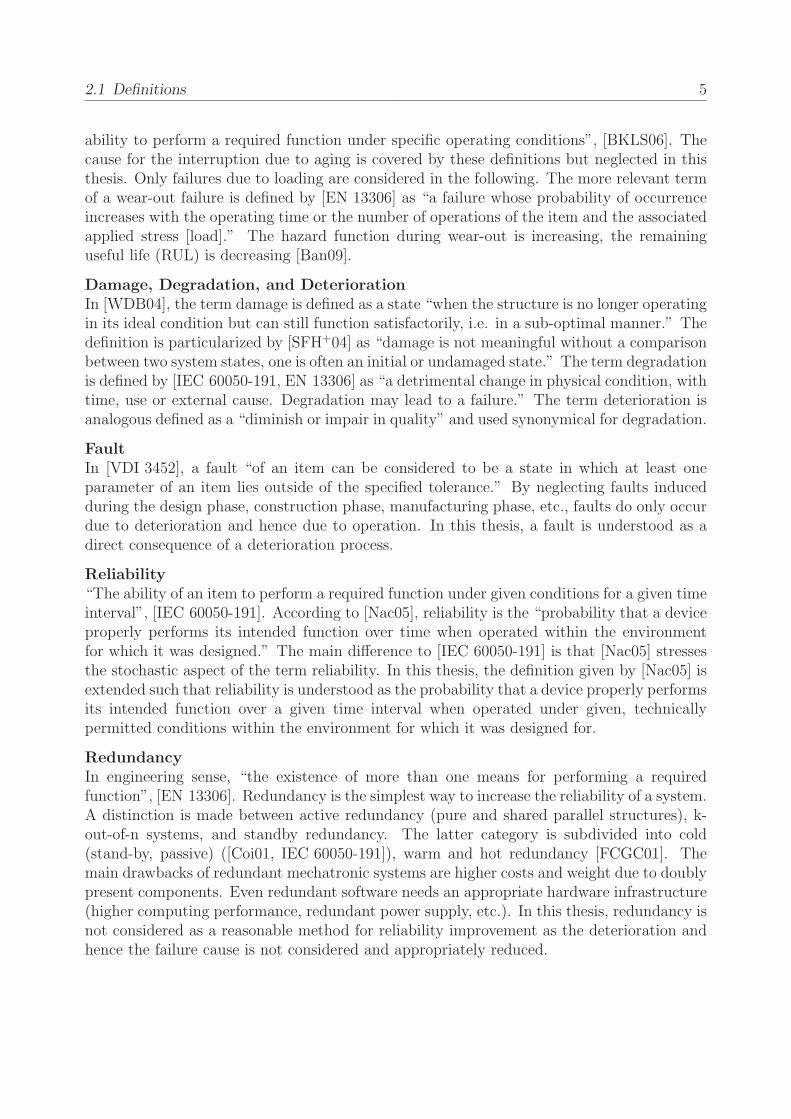
Based on these information, appropriate methods are available to investigate the future re-liability of a system. The common way in reliability analysis starts with a model of theinterdependencies (consisting of its function-relevant components). Subsequently, the in-dividual failure distributions are estimated, based on the above mentioned strategies forfailure distributions. For repairable components, Markov methods are commonly used. Fornon-repairable components, the Reliability Block Diagram (RBD) is usually more suitableto describe the function of a system. The symbols, terms and definitions are chosen accord-ing to [DIN EN 61078]. The RBD of a sample system, consisting of an architecture withcomponents in serial and parallel connection, is depicted in Figure 2.4.
2.2 Reliability Analysis 12
1
1
2
2
3
3
Figure 2.4: Reliability Block Diagram for a sample system
From this representation, the critical path, the most unreliable component, etc. can beidentified. The exemplary calculation of a non-repairable system depicted in Figure 2.4according to [RH04] is briefly shown in the following to illustrate the general scheme ofreliability calculation.The structure function of the depicted 2-out-of-3 structure is
φ(p(t)) = p1(t)p2(t) ∪ p1(t)p3(t) ∪ p2(t)p3(t)
= p1(t)p2(t) + p1(t)p3(t) + p2(t)p3(t)− 2p1(t)p2(t)p3(t) , (2.19)
with pi denoting the individual failure probability of each component i, pi = 1 denoting afully functioning component, whereas pi = 0 denotes a failed component at the consideredtime instant t. Hence, the structure function φ(p(t)) is equal to 0 if at least 2 componentsfailed.The survival function results to
RS(t) = R1(t)R2(t) +R1(t)R3(t) +R2(t)R3(t)− 2R1(t)R2(t)R3(t) . (2.20)
For simplicity, the reliability of each component is assumed as identical Ri(t) = R(t) fori = 1 . . . 3. With Equation (2.16), the reliability of the 2-out-of-3 system is
RS(t) = 3 exp(−2λt)− 2 exp(−3λt) . (2.21)
Hence, suggestions about improvements are derived in terms of more reliable components,redundancy structures, less components, etc. The effect of these actions can be calculatedand appropriate measures for reliability improvements can be initiated. These suggestionsare basically helpful during the design phase, revision activities (“facelift” in automotivesector), or maintenance planning. For an existing system, only the latter aspect forms a fea-sible solution for classical reliability improvement. In [VDI 4008, RH04], a comprehensiveintroduction to the most relevant reliability methods are given, namely Fault Tree Analysis(FTA), Markov chain, and Bayesian models. For comprehensive studies on reliability deter-mination and novel scientific applications, the European Safety and Reliability Association(ESRA) reveals an exhaustive collection of further methods and approaches to reliability

2.3 General Measurement Chain 13
Transducer Amplifier A/D-Converter CPU
DigitalElectricalElectricalMeasurandNorm.
SignalSignalSignal
Figure 2.5: Basic components of general measurement chain
engineering and related topics in their annual conferences ESREL. Additionally, the Inter-national Journal of Reliability, Quality and Safety Engineering (IJRQSE) is a relevant sourcefor reliability-concerned issues.
2.3 Measurement Chain for Acquiring Deterioration-InherentSignals
The challenge of measuring continuously (deterioration-inherent) signals with a non-destruc-tive concept is detailed in the following. In general, the measurement chain provides theinterface between the (physical, electrical, etc.) quantities and their digital correspondents(signals) and covers all relevant measurement components. In analogy to [DIN 1319], thegeneral measurement chain is depicted in Figure 2.5.At the outset of developing a novel measurement chain, the relevant measurands (physical
properties) are identified. This is realized by material examinations, field failure examina-tions, expert judgments, heuristic knowledge about the physics of failure, etc. The aim isto identify the physical, deterioration-concerned properties that cause the fault and failure,respectively. The measurement itself must not influence the measurement result and/or sys-tem. If the physical properties are directly measurable, the deterioration itself is directlymeasurable. Hence, appropriate transducers are applied to convert the deterioration into adigital signal. In general, the sensitivity of the measurement chain to marginal damages isa challenging task [Fri10].In the common case, the deterioration properties are locally distributed (e. g., surface
roughness of plate) and/or are not directly measurable (e. g., chemical reaction in accumu-lator). Then, surrogate properties are measured that correlate with the real deteriorationproperties. The indirect measurements presuppose that the surrogate quantities containdeterioration-relevant information. The connection between the surrogate quantities andthe real properties is realized by a filter. In summary, relevant physical properties (either di-rect or surrogate quantities) are measured by appropriate transducers (or complete sensors)to transform these into electrical signals.In general, a sensor is a functional element which connects a (non-)technical process (e. g.,
technical, chemical, biological) with an information processing unit (e. g., CPU). The prin-ciple of measurement assumes the existence of a reproducible, known relation between themeasurand (its physical effect, phenomenon) and the surrogate quantity. The linearity be-tween both is desirable due to less effort during the filtering process. As every sensor isan energy converter, it usually consists of a transducer and an amplifier. The transducerhas to respond to a physical property by converting the (non-)electrical measurand into anappropriate electrical signal. It provides directly measurable information about a measurandin terms of quantity, condition or property. The electrical signal can be a voltage, current

2.3 General Measurement Chain 14
or charge. The amplifier has to be electrically compatible with the output signal of thetransducer. Additionally, the electrical circuit of the amplifier must not change the electricalsignal waveform, e. g., by a noisy power supply, nonlinear transfer behaviors, power loss, notmatching input impedance, etc.Ideally, the principle of measurement is highly sensitive to the considered measurand
only. In practice, different (unknown) quantities influence the conversion process. Therefore,countermeasures for suppressing noise, reducing signal attenuation, increasing robustness,etc. are applied. Commonly, this is realized by, e. g., integrating the transducer and amplifierinto a customized housing.In general, sensors are classified according to different criterion, e. g., field of application,
principle of measurement, energy consumption, costs, etc. In [DIN 1313, DIN 1319], therelevant information about the fundamentals of metrology are given.Following [Whi87], an abridgment about a classification scheme for sensors is given in
Table 2.1.As shown in Figure 2.5, the normalized electrical signal is digitized by an analog-to-digital
converter (ADC) and passed to the CPU. An ADC digitizes an analog input signal into aseries of time and value-discrete values. The quantization in time denotes the resolution intime and is commonly expressed by a sample rate. The conversion is realized by keepingthe analog value constant for one time step (sample-and-hold element) and passing it toan high-impedance ADC. Then, the ADC quantizes the analog value into an digital value.The resolution is generally expressed in number of bits. Again, the electrical specification(in terms of bandwidth, electrical compatibility, response time, etc.) have to be adapted tothe output of the amplifier, the input of the information processing unit (CPU), and thedesired resolution for further examinations (filters, etc.). The particular practical challengesare detailed in Sections 4.2 and 5.2.As the measurement chain is the base for all subsequent investigations, special care has
to be taken by choosing, applying, and operating the equipment and components. To en-sure reliable and reproducible measurements, the following aspects have to be considered inadvance: The measurement chain
• must not affect the process itself (no feedback),
• withstand aggressive substances, environmental conditions,
• cover deterioration-relevant signals,
• measure relevant physical/chemical/... effect(s), and
• must be robust against measurement noise.
In anticipation of Chapters 4 and 5, relevant standards for piezoelectric ceramics and theiroperations are [DIN 50321-1, DIN 50321-3] as well as [DIN EN 60254] and [IEC 60050-486]for electrical measurements considering accumulators.In summary, the measurement chain provides the digitized signals (raw data) to subsequent
signal processing steps, e. g., fault detection and diagnosis algorithms. Commonly, measur-ments are involved as process inputs (operational parameters) and outputs (deterioration-inherent signals) have to be processed. The measuring principle has to be non-destructiveand the signals have to be measured continuously and with low noise.

2.4 Fault Detection 15
Measurands
Wave amplitude, phase, spectrum, etc.Acoustic Wave velocity
OtherCharge, Current
Electric Electric field (amplitude, phase, polarization, spectrum)OtherPosition (linear, angular)
Mechanical VelocityOther
Detection Means used in Sensors
Electric, Magnetic, Electromagnetic WaveMechanical Displacement or WaveOther
Technological Aspects of Sensors
SensitivityMeasurand rangeStability (short-term, long-term)ResolutionSelectivityOthers
Table 2.1: Classification aspects for sensors [Whi87]
2.4 Fault Detection
The task of fault detection is to evaluate the deterioration-related deviation from a nominal,a priori known behavior. The central prerequisite is that the deterioration mechanism effectsthe measured and/or numerically derived quantities. The evaluation can either be realizedby model- or signal-based methods.In general, quantities are defined according to their direction of action: an input covers
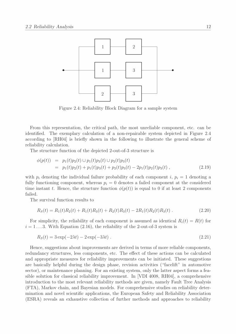
everything that acts on a system, whereas an output is defined as the causal reaction ofa system to an input. Hence, the system itself is driven by the inputs and reacts withcorresponding outputs, as depicted in Figure 2.6. The measured inputs u and outputs ycan either be continuous or discrete in time and/or values. For reasons of simplicity, theindication t for time-continuous and k for time-discrete systems are omitted in the following.Unless otherwise stated, all considerations are applicable for both, time-continuous and time-discrete approaches. Vectors and matrices are indicated by a bold notation.In dependency on the availability and applicability of a sufficiently exact mathematical
description of the system, its complexity, real-time demands, etc., an appropriate methodfor fault detection has to be chosen. The relevant methods are classified into two categories:model- and signal-based methods.
2.4 Fault Detection 16
u ySystem
FaultsFaults
Signal-basedModel-basedFault DetectionFault Detection
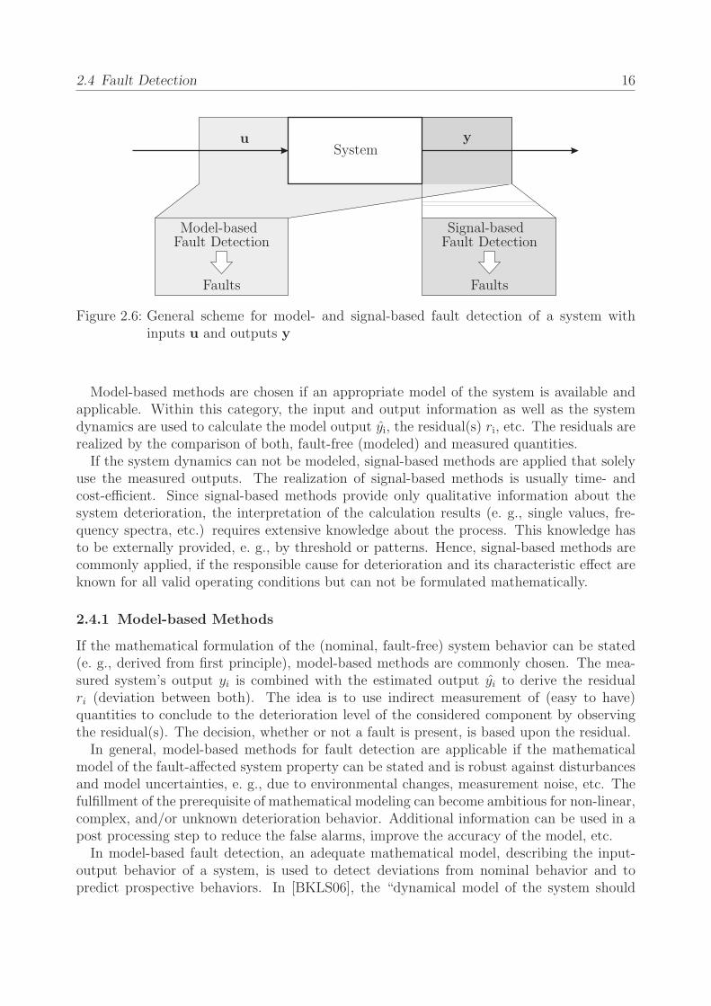
Figure 2.6: General scheme for model- and signal-based fault detection of a system withinputs u and outputs y
Model-based methods are chosen if an appropriate model of the system is available andapplicable. Within this category, the input and output information as well as the systemdynamics are used to calculate the model output yi, the residual(s) ri, etc. The residuals arerealized by the comparison of both, fault-free (modeled) and measured quantities.If the system dynamics can not be modeled, signal-based methods are applied that solely
use the measured outputs. The realization of signal-based methods is usually time- andcost-efficient. Since signal-based methods provide only qualitative information about thesystem deterioration, the interpretation of the calculation results (e. g., single values, fre-quency spectra, etc.) requires extensive knowledge about the process. This knowledge hasto be externally provided, e. g., by threshold or patterns. Hence, signal-based methods arecommonly applied, if the responsible cause for deterioration and its characteristic effect areknown for all valid operating conditions but can not be formulated mathematically.
2.4.1 Model-based Methods
If the mathematical formulation of the (nominal, fault-free) system behavior can be stated(e. g., derived from first principle), model-based methods are commonly chosen. The mea-sured system’s output yi is combined with the estimated output yi to derive the residualri (deviation between both). The idea is to use indirect measurement of (easy to have)quantities to conclude to the deterioration level of the considered component by observingthe residual(s). The decision, whether or not a fault is present, is based upon the residual.In general, model-based methods for fault detection are applicable if the mathematical
model of the fault-affected system property can be stated and is robust against disturbancesand model uncertainties, e. g., due to environmental changes, measurement noise, etc. Thefulfillment of the prerequisite of mathematical modeling can become ambitious for non-linear,complex, and/or unknown deterioration behavior. Additional information can be used in apost processing step to reduce the false alarms, improve the accuracy of the model, etc.In model-based fault detection, an adequate mathematical model, describing the input-
output behavior of a system, is used to detect deviations from nominal behavior and topredict prospective behaviors. In [BKLS06], the “dynamical model of the system should

2.4 Fault Detection 17
not only describe the faultless, but also the faulty system for all faults [...].” Accordingto [MEC02], “modeling begins by developing deterministic physical/chemical models for thefailure mechanisms. Then random and stochastic process distributions can be added [...] toaccount for important process variabilities.” That means that all fault-relevant dynamicsmust be considered during modeling. The model accuracy is subsequently evaluated bysimulation (verification) or experiments (validation).Following [SRA+08], model-based methods are divided into two groups, law-driven and
data-driven models. Other categorizations of the term model are known from literature,e. g., [Bel98].
Law-Driven ModelsThe following modeling techniques focus on an estimation of the measured, fault-relevantinput-output behavior by appropriate mathematical models (in terms of a set of mathemat-ical equations). These models have to represent sufficiently the system’s behavior with afinite number of parameters [Nel01].For linear, time-invariant systems with m inputs u and r outputs y, the input-output
behavior can be modeled as a set of ordinary differential equations [Lun08]
n∑
j=1
aijdjyidtj
=m∑
k=1
q∑
l=1
bkldluk
dtl, (i = 1, 2, . . . , r) , (2.22)
with aij and bkl as the time-invariant coefficients of the derivatives of the output and input,respectively. The index n denotes the system order and the maximum order of derivative ofthe output y( · ) where q represents the maximum order of the derivative of the input u( · ).The variables i, j, k, and l are continuous indices.The initial conditions
djyidtj
(0) = y0,ij , (i = 1, 2, . . . , r and j = 0, 1, . . . , n− 1)
have to be known.It is obvious that the description of the input-output behavior by differential equations,
especially for systems with multiple inputs and/or multiple outputs, can become very com-plex. Hence, the system dynamics is represented in the state space. For linear continuoussystems, described in time domain, the state space description is defined as
x = Ax+Bu , (2.23)
y = Cx+Du , (2.24)
with x representing the states of the system’s dynamic in dependency on the time, u cor-responding to the inputs to the systems, and y describing the outputs of the system. Thesystem matrix A represents the dynamics and couplings of the system. In combination withthe input matrix B, describing the influence of the input vector u on the system dynamics,Equation (2.23) is called the dynamical equation. The output equation (2.24) consists of thematrix C, mapping the states x to the output y, and the matrix D, realizing the direct feedthrough of inputs u on the output y.In the following, the two common mathematical models for fault detection purpose are
introduced. An overview about available methods is given in [Ise06].

2.4 Fault Detection 18
u y
System
Observer
A
B C
B
A
C
∫
∫
L
x
−
x
˙x x y
e r
Figure 2.7: General scheme of Luenberger observer
• State ObserverIn general, a state observer reconstructs internal states from measured states on basisof a mathematical model and known model parameters. For diagnosis purpose, theobserver uses measurable states (system’s outputs y) in order to conclude to internalstates x that are not directly measurable. In Figure 2.7, the general scheme of a systemwith an observer in parallel is given.
The standard Luenberger observer [Lue64] is described by
x =(A− LC
)x+ Ly , (2.25)
y = Cx , (2.26)
with D = 0. The hat notation indicates the observer matrices and signals.
The mathematical prerequisite for the applicability of an observer is the observabilityof the considered system model, which means that immeasurable states can be recon-structed from measurement of outputs and thus, eigenmotions can be reconstructed.

2.4 Fault Detection 19
For systems with few states, the observability is proven if theKalman criterion [Kal60]
rank (Qo) = rank
CCA...
CAn−1
!= n , (2.27)
is fulfilled.
To obtain a high observer performance, a high-gain L is usually chosen [Lun08, Kha02].As a result, the residual r decays rapidly. The main drawbacks of this approachare a high sensitivity against measurement noise and model and/or parameter errors.Additionally, peaking is a commonly known challenge for high-gain observers thatresults in high corrective actions and thus, overshooting of y [Kha02].
Hence, the determination of an appropriate observer gain L is the main challenge forthe observer design. The gain has to be chosen such the observer is faster than thereal system which is realized by the location of the eigenvalues of the observer. Acommon measure for a sufficiently fast response of the observer is obtained by placingthe eigenvalues three to ten times faster than the dominating eigenmotions of theobserved system [Lun08].
The model is simulated in parallel to the real system. As introduced above, the resid-uals r (deviation between measured output y and calculated output y) are used asan indicator for fault detection. A fault is defined as an intersection of the residual(one or several values) during the observation with a predefined lower or upper limit.Hence, the residual evaluation is a rule-based method in order to detect faults. Theinterpretation of the connection between cause and responding residual must be found.
In [HS09], an example for observer-based fault detection is proposed. The methodis applied to an elastic mechanical system (cantilever beam) for the localization ofcracks. A (increasing) deterioration is assumed to act as an additional input (virtualforce) on the system and hence, disturbing the nominal behavior. The solution of theinverse problem reveals fault-relevant information about the unknown force and fault,respectively.
In [FK06], an observer-based method for unknown input identification is proposed. Thefilter (law-driven model) is an analytic model (Finite Element Model) of the structurethat reconstructs external inputs (forces) to the system from measured structural re-sponses (accelerometer and strain gauges).
• Parity EquationsSimilarly to the observer technique, the parity space equations are based on the eval-uation of the computed and measured signals.
Here, models with known structure (commonly in state space representation) but un-known parameters are used. The parameters of the model are estimated based on themeasured input and output data. Subsequently, the estimated parameters are usedto simulated the model behavior, based on measured inputs. The general scheme issimilar to the one, shown in Figure 2.7 except for the feed back of the error e to the

2.4 Fault Detection 20
observed state x. As this branch is omitted, no considerations about observability andstability have to be carried out. Only the parameters of the model have to be identifiedwhich is typically formulated as an optimization task. Typical methods for parame-ter estimations are the Least Squares Estimation (LSE) and the Maximum LikelihoodEstimation (MLE), detailed in Section 3.4.
In [Kas06], parity equations and an observer are used in parallel as virtual sensors tosupervise a system. By merging these information to so called symptoms, the faultdetection sensitivity is improved. The post processing step (subsequent filter) can berealized by a fuzzy-based method.
Both law-driven models base on a mathematical model, commonly derived from first prin-ciple. From a diagnostic point of view, the main difference between the proposed approachesis the importance of the parameters. The parameters of the observer are derived from mea-surement and satisfy the physical equations (in terms of units, physically correct values, etc.).If the system is observable, the observer gain L has to be designed such that the observerreacts sufficiently fast and stable in order to calculate the output (placement of eigenvalues).This numerically complex procedure can be avoided by using the parity equations. Withinthis approach, the parameters are estimated by standard algorithms in order to reproducethe input-output behavior. The drawback is that the estimated parameters have no physi-cal meaning but only satisfy the optimization task. Hence, a cross-link between estimatedparameters and physical quantities is only possible by using an observer technique.
Data-Driven ModelsIn contrast to law-driven approaches, the data-driven models do not depend on predefinedmathematically formulated laws but derive the input-output relation from observations (e. g.,measurements). As stated in [YPL96], these models “can describe reality with a minimum ofadjustable parameters.” Furthermore, data-driven models are commonly used in the domainof non-linear systems, where most systems and/or behaviors occurring in nature are non-linear. A non-linear system performance is present if either the principle of superpositionand/or the principle of homogeneity are not fulfilled and/or do not apply. The non-linearitycan occur in the function(s) and/or the arguments. Non-linear models need an infinitenumber of parameters, in order to describe a system and/or its dynamics (see [Nel01]). Suchmodels are realized typically by means of interpolation data, set of curves, characteristicdiagrams, neural or Wavelet nets, etc. These models require preliminary information neitherabout the physical behavior of the considered system nor about its physical parameters.
• Artificial Neuronal Net (ANN)An ANN is composed of inputs that are connected via numerous individual neuronswith the output(s). The information transfer is realized by a directed communicationbetween the individual neurons. By connecting and organization these neurons intogroups, so called (input, hidden, and output) layers of the ANN are obtained. Acomprehensive introduction into ANN is given, e. g., in [Bis94].
The ANN has to be trained first to reproduce the input-output behavior (supervisedlearning). Subsequently, the training result is tested on the basis of different (un-trained) inputs. If the calculation results correspond sufficiently with a representativenumber of untrained input-output behaviors, the net is used for detection purposes.

2.4 Fault Detection 21
Otherwise, the net must be further trained or additional layers and/or activation func-tions etc. have to be added/modified. An ANN can be adapted to almost every systemwhether it is linear or non-linear without phrasing the inner (fault) dynamics mathe-matically. The disadvantage of this method is that the generated model has no physicalequivalent; the layers can not be interpreted and correlated with physical parameters.
• Fuzzy LogicWhere the well-known Boolean Logic only discriminates between two states, 0 (false)and 1 (true), the Fuzzy Logic extends the discrimination to a continuous range between0 and 1. Fuzzy Logic is commonly applied if a continuous quantity has to be assignedto different states. This assignment is realized by (overlapping) membership functions.
For fault detection purposes, Fuzzy Logic is usually applied to evaluate residuals.However, the Fuzzy Logic (basically if-then rules) can be trained by numerical dataand the support of ANNs. The advantage over the ANN method is that the modelcan be both, accurate enough and interpretable. In dependency on the degree ofcomplexity, the Fuzzy Logic can combine the ability to learn from measured data andto reveal relevant input-output connections. Hence, an insight into the unknown innerstructure (physical behavior) of the supervised system can be obtained [Mor05].
In [MMS+03], a state of damage of a combustion engine is based on the measured lubri-cation contamination by wear debris. The deterioration is subsequently estimated by amathematical data-driven Fuzzy Logic that assigns the measured debris concentrationto a level of deterioration.
Subsequently, the validation proofs the validity of the derived model within predefinedlimits. Normally this is done by propagating uncertainties in the input values, model pa-rameters, etc. through the model. Typical simulation methods are either Monte-Carlosimulation (assuming distributed input parameters, derived from observation and/or esti-mation) or Bayesian analysis. By evaluating the deviation of the estimated and observedoutputs, information about the fault’s confidence (interval) are obtained.
2.4.2 Signal-based Methods
For systems with simple or highly complex (non-linear) inner dynamics, unknown inputs, etc.signal-based methods are used that do not base on the exact, mathematically formulatedinput-output behavior of the system. The calculation results vary from single values tofrequency spectra. Thus, the subsequently introduced methods are subdivided into twomajor categories: time domain methods and (time-)frequency domain methods.
Time Domain MethodsFor many safety relevant systems, supervision of a threshold value is required to realize anemergency stop function. In [JW06], the temperature of an accumulator is supervised bya sensor. A rapid change of the cell temperature and threshold crossing is interpreted asa failure and the operation of the cell is terminated immediately. Here, the supervisionof one measurand is sufficient to conclude qualitatively to an extensive deterioration. Theknowledge about this correlation is derived from an heuristic knowledge base. A model-based method could be applied here as well, but the signal-based method is more robust,

2.4 Fault Detection 22
easy to have, and reliable. The interpretation of a variation of temperature from nominalbehavior requires a knowledge base, which can be provided as a look-up table derived frombaseline tests, etc. The temperature development over system usage can then be used asa deterioration indicator for fault detection. Commonly, solely signal-based methods arelimited to stationary processes. Otherwise, thresholds have to adapted for varying workingpoints, operating conditions, etc.In dependency on the particular domain, the following methods are commonly applied.
• Threshold MonitoringThe threshold value analysis is the simplest method for fault detection. A fault isdetected as soon as a predefined limit is intersected. For the threshold value anal-ysis there is a multiplicity of typical application possibilities, like the monitoring oftemperature, current flow, pressure, force etc.
• Trend EstimationFor a system under constant operation, this method is applied to reveal the tendencieswithin the considered time data. In combination with statistical measures, signals fromrandom and faulty behavior can be separated from each other.
The cycle-counting algorithm by [DS82], rainflow-counting algorithm by [ME68], etc.are algorithms to count the occurrence of events versus an operation phase. Theobtained histogram (e. g., rainflow-matrix), can found the base for separating normaland abnormal behaviors. Especially for the analysis of fatigue data, the rainflow-counting algorithm is used.
Beside the direct evaluation of time data, statistical quantities can be supervised bythe method as well. This is relevant for systems under repetitive operation, wheretrends between results at identical set point operations can be compared.
(Time-)Frequency Domain MethodsThe (Time-)Frequency analysis is performed if deterioration-relevant information are as-sumed to characteristically and uniquely influence the frequency spectrum and “are usedto analyze non-stationary events”, [Fri10]. All following methods decompose periodic andnon-periodic signals into single harmonic sinusoid functions.
• Fourier Transformation (FT)The Fourier Transformation F of a signal y(t) is expressed by [BSMM05] as
F (ω) = Fy(t) =
+∞∫
−∞)
y(t)e−iωtdt . (2.28)
As the frequency content of non-stationary signals will be examined later on, the time-discrete realization of the Fourier Transformation is given by
yD(iω) =N−1∑
k=0
y(kT0)e−iωkT0 (2.29)

2.5 Fault Diagnosis 23
whereN describes the number of samples at discrete time instants (e. g., measurements,data points, etc.) and T0 represents the sampling interval [Ise06]. Therefore, thecontinuous sequence y(t) is split into several sequences, each of identical length N .To avoid aliasing effects, appropriate non-overlapping window functions are applied.These window function modify the signal such that the signal is reduced to zero at itsinterval boundaries k = [0, N − 1]. Thus, no discontinuities arise from the windowing.
In the case of a present fault, the evaluation of fault-sensitive signals reveals the devi-ation from the nominal behavior and is thus applicable for fault detection purposes.
• Short Time Fourier Transformation (STFT)The consecutive calculation of the FT results in a temporal succession of spectra fromshort time intervals. This kind of transformation is called Short Time Fourier Trans-formation (STFT) and preserves the time information within the frequency analysis.In dependency on the chosen overlapping strategy, the single Fourier Transformationare lines up or overlapping. The advantage of the STFT in comparison to a FT is thatalso transient signals can be transferred into a time-dependent frequency spectrum. Awindow w function, commonly a Hann window, is introduced in Equation (2.28) andthe STFT is obtained as
ySTFT (iω) =
+∞∫
−∞)
y(t)w(t− τ)e−iωtdt . (2.30)
The parameter τ indicated the time instant of interest.
Unfavorable is that the detectability of a transient signal is depended with regard tothe chosen length N of discrete values. High frequencies (relative to the fundamentalfrequency) appear less dominant in the spectrum than lower frequencies.
In summary, fault detection evaluate the deterioration-related deviation from a nominal, apriori known behavior. The decision, whether a model- or signal-based method is applicableis only depending on the feasibility of setting up a model for the deterioration-affected input-output behavior or deterioration mechanism, respectively. If the inputs can be assignedby a mathematically formulated model to the deterioration-affected outputs, then model-based methods are chosen as these reveal direct deterioration-proportional faults and allowhigher level reasoning. If this requirement is not fulfilled or the system dynamics are toocomplex (e. g., non-linear), signal-based methods are applied. The obtained faults yield rawinformation about upward/downward trends of values, changed frequency contents, etc.
2.5 Fault Diagnosis
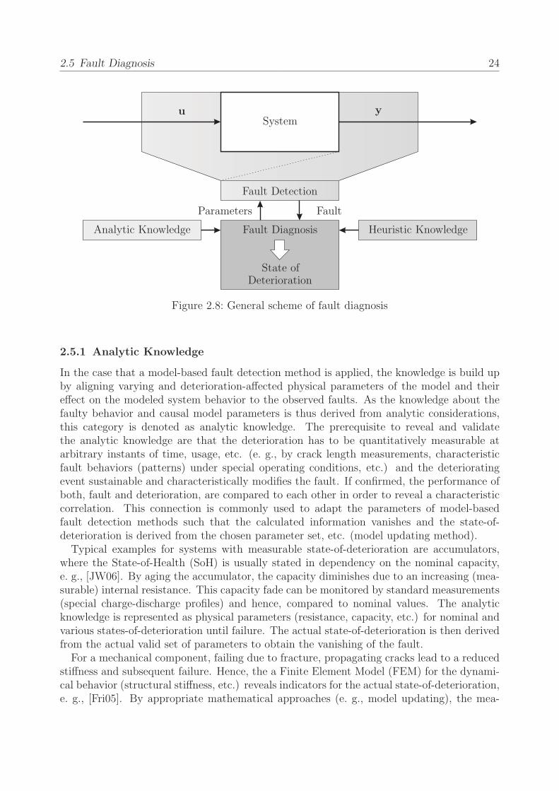
The task of fault diagnosis is to evaluate the detected fault in order to determine the originof deviation and thus, correlating the fault to the resulting state-of-deterioration. Hence,the fault diagnosis is the subsequent step to fault detection; the relation between both isdepicted in Figure 2.8. The required knowledge to interpret the fault has to be provided,e. g., in dependency on the performance of the fault, available information, etc. Accordingto the source of knowledge, the fault diagnosis methods are divided into two categories.
2.5 Fault Diagnosis 24
u ySystem
FaultParameters
State ofDeterioration
Heuristic KnowledgeAnalytic Knowledge
Fault Detection
Fault Diagnosis
Figure 2.8: General scheme of fault diagnosis
2.5.1 Analytic Knowledge
In the case that a model-based fault detection method is applied, the knowledge is build upby aligning varying and deterioration-affected physical parameters of the model and theireffect on the modeled system behavior to the observed faults. As the knowledge about thefaulty behavior and causal model parameters is thus derived from analytic considerations,this category is denoted as analytic knowledge. The prerequisite to reveal and validatethe analytic knowledge are that the deterioration has to be quantitatively measurable atarbitrary instants of time, usage, etc. (e. g., by crack length measurements, characteristicfault behaviors (patterns) under special operating conditions, etc.) and the deterioratingevent sustainable and characteristically modifies the fault. If confirmed, the performance ofboth, fault and deterioration, are compared to each other in order to reveal a characteristiccorrelation. This connection is commonly used to adapt the parameters of model-basedfault detection methods such that the calculated information vanishes and the state-of-deterioration is derived from the chosen parameter set, etc. (model updating method).Typical examples for systems with measurable state-of-deterioration are accumulators,
where the State-of-Health (SoH) is usually stated in dependency on the nominal capacity,e. g., [JW06]. By aging the accumulator, the capacity diminishes due to an increasing (mea-surable) internal resistance. This capacity fade can be monitored by standard measurements(special charge-discharge profiles) and hence, compared to nominal values. The analyticknowledge is represented as physical parameters (resistance, capacity, etc.) for nominal andvarious states-of-deterioration until failure. The actual state-of-deterioration is then derivedfrom the actual valid set of parameters to obtain the vanishing of the fault.For a mechanical component, failing due to fracture, propagating cracks lead to a reduced
stiffness and subsequent failure. Hence, the a Finite Element Model (FEM) for the dynami-cal behavior (structural stiffness, etc.) reveals indicators for the actual state-of-deterioration,e. g., [Fri05]. By appropriate mathematical approaches (e. g., model updating), the mea-

2.6 Failure Prognosis 25
sured (locally) reduced stiffness can be traced back to localize and quantize the state-of-deterioration. A similar idea of solving the inverse problem of calculating from measuredeffect to cause can be realized by an observer, as described in [HS09]. This process usestechniques based on observed (known) input-output correlations (law-driven models).Furthermore, other methods for interpreting the connection between fault and (determin-
istic) deterioration are known in literature, e. g., neural nets (see Section 2.4.2), Bayesiannets, etc.
2.5.2 Heuristic Knowledge
In the case that the deterioration behavior is not available in analytic terms, a heuristicapproach is chosen to assign the faults to the state-of-deterioration. Especially, if stochas-tically occurring deteriorating events (temporarily) effect the (deterioration-inherent) fault,but a direct correlation between a state-of-deterioration and a shift, trend, or exact (ab-solute) value of fault is not possible since immeasurable, fault diagnosis based on heuristicknowledge is applied. The relationship between deteriorating event and fault performanceare then derived from continuous supervision of fault shifts, etc.By designing appropriate test runs, heuristic knowledge is empirically derived from ob-
served failures. In dependency on the particular domain (mechanical, electrical, etc.) and(dominant) failure mechanism, a priori assumptions are used to support the evaluation ofthe measurements (known physical principles, etc.). Based on this knowledge, general load-failure connections (models) are established in order to approximate the deterioration be-havior (deterioration-proportional information).Therefore, the effect of the deterioration mechanism on the failure is investigated empiri-
cally and an heuristic knowledge (assumed effect of deterioration on failure) is build up whichincorporates information from process histories and failure statistics. Thus, the diagnosisbases on empirical data that reveal the correlation between the state-of-deterioration andthe detected failure.As the calculation can not be correlated with the real state-of-deterioration, the assump-
tions about the deterioration mechanism determine the calculation result. Due to the varioussources of uncertainties or limited number of measurements, the deterioration model can stillbe invalid or at least incomplete. To deal with these probabilities, probabilistic-based as-sumptions and validation test runs play a major role.
2.6 Failure Prognosis
The preceding sections deal with the challenges in determining the actual state-of-deteriora-tion. In failure prognosis, the prospective deterioration is considered and hence to supportthe choice of deterioration-optimal parameters. “The highest and most sophisticated level[of damage assessment] is the prognosis of the remaining useful life” [Fri10], where theRemaining Useful Life (RUL) is “the operating time between a certain time instant and anunacceptable level of degradation”, [Sye10].In contrast to fault diagnosis, the prognosis extends the consideration to the task of cor-
relating the operational parameters with the resulting state-of-deterioration. In order tomaximize the remaining useful life and hence, minimize the deterioration of a system, sur-rogate models are used to estimate the most probable deterioration behavior of a system

2.6 Failure Prognosis 26
u ySystem
Fault Detection
Faults
Fault Diagnosis Knowledge
Parameters
State ofDeterioration
Reliability TargetsFailure Prognosis
Operat.
Targets
Figure 2.9: General scheme for a reliability-supervised system
for a given (known) input trajectory (operational parameters). These models have to con-sider the actual state-of-deterioration, assumptions about the future deterioration (behavior)within predefined confidence limits, the past and prospective operational conditions, and therequired reliability targets. Several methods, describing an input-output behavior, are intro-duced above and applicable here (e. g., Neural Nets, (Neuro-)Fuzzy approaches, ARMAXmodels, etc.).The novel aspect of approximating the propagation (time evolution) of faults and hence,
instant of failure as a consequence of the prospective deterioration behavior is addressedin this section. The scheme of diagnostic-based failure prognosis and control is depicted inFigure 2.9.This chapter comprises the key challenges for failure prognosis and introduces the theo-
retical foundations for multi-dimensional models to approximate the response of a system(life time, deterioration, etc.) due to the applied (independent) operational parameters. Itis assumed in the following that statistically sufficient samples of failure data sets (past op-erational profiles and associated deterioration) are available to support the training of themodels.First, the idea is illustrated of how to design appropriate test runs that reveal the required
information of appropriate operational parameters for each identified operational (deteriora-tion) phase. Then, a functional relationship is identified that ties together the loading andthe aging and hence closes the gap between deterioration measurement and deteriorationcontrol.

2.6 Failure Prognosis 27
Length of Test Specimen [mm] ξ1 250 350Amplitude of Load Cycle [mm] ξ2 8 10Load [N] ξ3 40 50
Normalized Factors xi −1 +1
Table 2.2: Operational parameters of a sample system and assignment to normalized fac-tors [BDHH07]
2.6.1 Design of Experiment (DoE)
The primer task of test design is addressed by the Design of Experiments (DoE) [Mon09,BHH05, BDHH07] in order to obtain the required test results within a minimum numberof test runs. The secondary aim of DoE is to avoid redundant, meaningless tests, and longtest periods by appropriately designing the test matrices and procedures. The importantfactors (operational parameters) that have a major influence on the deterioration are knownfrom previous investigations. Additional methods, e. g., sensitivity analysis can be appliedto support this investigation step and to focus on the significant (in terms of usage control)parameters (factors). A first approach is the observation of typical parameter sets and theirnumber of occurrence during a representative test period.At the exploratory stage of the test design, a parameter sub-space of the possible parameter
space (spanned by all independent operational parameters) is selected to reveal significantresults about the relationship between load and deterioration. Subsequently, the relevantrange (value limits) of each parameter is determined. Again, the search space is restricted toan explicit sub-space of operational parameters in order to rapidly reveal a first insight intothe system behavior. Based on the obtained results and conclusions, adjacent investigationsaugment the test matrices and thus, the parameter sub-space.In the following, a system with three independent operational parameters u is consid-
ered that is operated under various operational conditions until failure. In Table 2.2, theoperational parameters with their relevant limits are given.As the method of DoE is independent of the type and source of operational (physical) pa-
rameters u (quantitative and/or qualitative sources can be mixed), normalized factors x areused instead, which are linear transformations of the original measure. The transformationsfor the operational parameters of the sample system are realized by
x1 =u1 − 300mm
50mm, x2 =
u2 − 9mm
1mm, and x3 =
u3 − 45N
5N. (2.31)
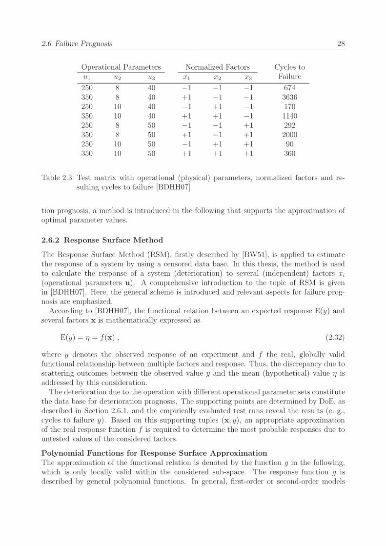
For the above introduced example with three independent factors x1, x2, and x3, a testmatrix with eight comparable systems, realizing all possible combinations of the normalizedfactors, is selected. The aging results are given in Table 2.3.Based on the results, subsequent test runs are designed appropriately. In dependency on
the aim of investigation, other parameter sets (extended limits, intermediate values, etc.)can be tested as well as additional operational parameters can be varied in order to extendthe data base.In summary, the method of DoE is a guideline to focus on the relevant test runs. In
combination with few but relevant failure tests, constituting the data base for deteriora-
2.6 Failure Prognosis 28
Operational Parameters Normalized Factors Cycles tou1 u2 u3 x1 x2 x3 Failure
250 8 40 −1 −1 −1 674350 8 40 +1 −1 −1 3636250 10 40 −1 +1 −1 170350 10 40 +1 +1 −1 1140250 8 50 −1 −1 +1 292350 8 50 +1 −1 +1 2000250 10 50 −1 +1 +1 90350 10 50 +1 +1 +1 360
Table 2.3: Test matrix with operational (physical) parameters, normalized factors and re-sulting cycles to failure [BDHH07]
tion prognosis, a method is introduced in the following that supports the approximation ofoptimal parameter values.
2.6.2 Response Surface Method
The Response Surface Method (RSM), firstly described by [BW51], is applied to estimatethe response of a system by using a censored data base. In this thesis, the method is usedto calculate the response of a system (deterioration) to several (independent) factors xi
(operational parameters u). A comprehensive introduction to the topic of RSM is givenin [BDHH07]. Here, the general scheme is introduced and relevant aspects for failure prog-nosis are emphasized.According to [BDHH07], the functional relation between an expected response E(y) and
several factors x is mathematically expressed as
E(y) = η = f(x) , (2.32)
where y denotes the observed response of an experiment and f the real, globally validfunctional relationship between multiple factors and response. Thus, the discrepancy due toscattering outcomes between the observed value y and the mean (hypothetical) value η isaddressed by this consideration.The deterioration due to the operation with different operational parameter sets constitute
the data base for deterioration prognosis. The supporting points are determined by DoE, asdescribed in Section 2.6.1, and the empirically evaluated test runs reveal the results (e. g.,cycles to failure y). Based on this supporting tuples (x, y), an appropriate approximationof the real response function f is required to determine the most probable responses due tountested values of the considered factors.
Polynomial Functions for Response Surface ApproximationThe approximation of the functional relation is denoted by the function g in the following,which is only locally valid within the considered sub-space. The response function g isdescribed by general polynomial functions. In general, first-order or second-order models

2.6 Failure Prognosis 29
are assumed to describe the response surface. Although higher-order models are possible aswell, these are seldom applied as the number of parameters increases significantly.The first-order model is described as
y = g(x)
= β0 + β1x1 + β2x2 + . . .+ βkxk + ǫ
= β0 +k∑
i=1
(βixi) + ǫ , (2.33)
with k denoting the number of inputs and βi the parameters to be identified by appropriatemethods.The second-order model for the locally valid response function g is expressed as
y = β0 + β1x1 + β2x2 + . . .+ βkxk + . . .
β1,1x21 + β2,2x
22 + . . . βk,kx
2k + . . .
β1,2x1x2 + . . . β1,kx1xk + . . . βk−1,kxk−1xk + ǫ
= β0 +k∑
i=1
(βixi) +k∑
i=1
(βi,ix
2i
)+
k∑
i=1
k∑
j=i+1
(βi,jxixj) + ǫ . (2.34)
The parameters of g are evaluated over the considered limits by appropriate approxi-mation procedures for fitting the empirical function g to the supporting tuples, e. g., bypolynomial fitting by maximum-likelihood, least squares, etc. According to [BDHH07], thetrue (unknown) underlying response function f can be approximated within this limitedregion sufficiently. Hence, it is possible to represent the relevant connection between factors(operational parameters) and response (resulting deterioration). “Although the approxima-tion can be far from perfect” [BDHH07], qualitative information can be derived from therevealed function (e. g., influence of single factors on deterioration, etc.), e. g., the direction(in terms of gradients) of factor modification in order to obtain a response-optimal value.
Application of First-Order Model to Sample DataFor relationships with up to three inputs (k = 3), the (piecewise, locally valid) functiong is graphically represented as a curve (two dimensional) or a plane (three dimensional),respectively to approximate the untested data points. For the higher-dimensional case (morethan three inputs u), geometric representations are not available to visualize the relationand is thus, realized numerically.Considering the data from Table 2.3, the parameters of the first-order polynomial from
Equation (2.33) are evaluated by the method of least squares such that
y = 1045.3 + 738.8x1 − 605.3x2 − 359.8x3 + ǫ . (2.35)
The surface for a constant value for the cycles to failure (exemplary assumed as 1000 cyclesto failure, colored in light-gray) is depicted in Figure 2.10.As narrow limits are chosen for the operational parameters, the approximation by a first-
order functional relationship can be sufficient to conclude to optimal operational parameters(in terms of maximum system usage).For deterioration prognosis, Equation (2.35) reveals the important information. As the
cycles to failure are investigated, the parameter set has to be determined that maximizes

2.6 Failure Prognosis 30
DecreasingAging
IncreasingAging
Response Surface forConstant Number ofCycles to Failure
IncreasingEfficiency
DecreasingEfficiency
Response Surface forConstant Efficiency
x1
x2
x3
−1
−1 −1
0
00
+1
+1
+1
Figure 2.10: Surfaces of deterioration (light gray) and efficiency (dark gray) response
the response y. It can easily be seen from the equation that the factor x1 has the largestimpact on the response. Hence, increasing x1 directly leads to an rapidly increasing numberof cycles to failure. Especially for systems with more independent operational parameterthan three (as considered here in this example), this information is essential to adjust themost sensitive operational parameters in the intended direction.The ultimate challenge to solve is, in which extend a modification (here: maximization
of factor x1) is contrary to additional conditions, e. g., process efficiency, product quality,etc. Hence, the objectives of the system (high throughput, minimum energy, minimumamount of material, reduced idle modes, etc.) have to be included in this considerationsto adequately modify the operation of the system and fulfill in parallel the objectives (ofproduction, functionality, etc.) Therefore, the response (here: efficiency) is derived by usingthe same operational parameters. The resulting plane is depicted in Figure 2.10 by the dark-gray colored plane. The intersection of both planes, representing the optimal parameter seton the one hand in terms of deterioration, on the other hand in terms of operation, revealsthe parameter constellation that comprises for both, deterioration and functionality.From this figure it is obvious that the operation is not optimal in terms of deterioration
but can be varied in order to increase the number of cycles to failure (decrease aging) by

2.6 Failure Prognosis 31
adjusting the parameters such that the aging plane is moved to the right until only oneintersecting point of both planes is obtained.In general, the optimum for each response may reveal conflicting setting. Hence, a balance
between the aging and the efficiency has to be found that reveals the most appropriate valuesfor all responses.Finally, the number of occurrence (of parameter sets) can be incorporated in this inves-
tigation as well (selection of sub-space, see Section 2.6.1). Thus, the distribution of typicaloperational parameter sets is evaluated. By fusing all this information, a comprehensiveoverview is obtained that forms the base for optimization.In summary, the method of RSM in combination with DoE provides a powerful measure
for optimizing the deterioration of a system by varying the relevant (or typical) operationalparameters and fulfilling in parallel production targets. The explicit formula, derived fromexperiments, is differentiable. Hence, the response can be maximized or minimized accordingto gradient examinations. This aspect is especially important to reveal an optimal trajectoryof inputs in accordance with an optimal response. Furthermore, detailed information aboutadditional, not yet accomplished test runs can be derived from this investigations to completethe data base.The location of the experimental region of most interest is identified and subsequent
test runs can economically fit a more elaborate model (in terms of degree of complexity,parameters, etc.) between the inputs and the response. This is especially important forthe design of further experiments. Conflicting goals (increasing input one leads directly toan unwanted decrease of input two) can be found within the investigation. Finally, theinvestigations can be supported by inputs, limited to predefined limits. An optimizationstrategy can subsequently be applied to reveal the appropriate input settings for a givengoal of response.

3 Novel Probabilistic-based Method for Modeling and
Controlling Systems’ Deterioration
Research within classical fault-tolerant control architectures addresses mainly the re-config-uration of the controller with regard to the functionality of the system. One example forthis interpretation of Fault Tolerant Control (FTC) is given in [BIMP04], where FTC for“a reconfiguring unit [...] adjusts the structure and the tuning of the controller in orderto preserve specified performances also for the faulty system.” A typical example of thecommon interpretation of fault-tolerant control is given by [BKLS06]. A model-based faultdiagnosis approach is “used to find remedial actions that adapt the control algorithms to thefaulty conditions in order to keep the system in operation.” The actual state-of-deterioration(classical SHM strategy) is thus estimated only with the help of model-based approaches,based on heuristic knowledge. Depending on the analyzed fault, the controller parametersand/or configuration are changed “to on-line re-design the controller” in order to adapt tothe faulty situation. The strategy of the control reconfiguration concentrated exclusively onmaintaining the functionality of the system to “satisfy the performance specifications”. Thisreactive strategy does not incorporate alternative operational strategies in order to preventfault development, but focuses on the “reconfigurability of the system or the search forredundant sensors and actuators, which can replace faulty components.” The sophisticatedaspect of controlling fault propagation is not addressed by this approach. Hence, a reliability-controlled system, based on the derived deterioration information, is not realized. Thenovel interpretation of fault-tolerant control selects appropriate operational parameters withregard to an extension of the life time and reduction of further deterioration.Generally, the life-time trajectory of a system is composed of a sequence of non-overlapp-
ing, distinct phases with particular deterioration behaviors. If the deterioration behaviordepends on the actual state-of-deterioration, these systems are called phased mission systems.Typical phases are the run-in phase, the permanent-wear phase, and the wear-out phase,as described by [San08] for fracture mechanics and [Jon09] for accumulators. Generallyspeaking, other classifications are possible; see, for example, [AB09], who divides the missionof an aircraft into the phases take-off, cruise, and landing. Other systems switch betweenoperational and maintenance phases, for example power plants.The challenge is to develop methods that consider the actual state-of-deterioration, the
previous loading history, the particular operational phases, and the time instant of investi-gation.The idea behind finding an adaptive compromise between safety, reliability, and costs over
the life time during field usage of a phased mission system is to control the affecting inputsignals (operational parameters) adequately. In this thesis, this key feature is subdividedinto three tasks which are based on one another: First, the connection between loading anddeterioration needs to be determined and expressed in an adequate mathematical model.Based on this knowledge, the operational parameters which affect the deterioration haveto be adapted in a deterioration-optimal way (while maintaining the functionality), and

3.1 Safety and Reliability Control Engineering Concept (SRCE) 33
finally, the appropriate countermeasures have to be initiated to reduce the probability offault occurrence.Besides the classical challenges of SHM, the novel aspect developed in this thesis is a
method to estimate the optimal operational parameters (determined by the actual state-of-deterioration) and their subsequent use for controlling the life time. The underlying,promising SRCE-concept [SR97] is explained in detail in the following section. Afterwards,the probabilistic part of the SRCE-concept, introduced by [Wol08], and its essential results,as derived from numerical studies, are briefly discussed.This thesis broadens the preliminary work by introducing novel aspects of appropriate
strategies for addressing and improving systems’ reliability. Additionally, the conceptualideas of the SRCE concept are brought into practice for the first time. The open tasks torealize the SRCE concept are refined in Section 3.2. They are divided into three modules,which will be adapted to special technical applications in Chapter 4 and Chapter 5. Partic-ular emphasis is put on modules 2 and 3, which realize the failure prediction, based on aninsufficient data base, and form the base for control strategies. The latter module in par-ticular is important for controlling the deterioration by adaptive operational strategies. Inthe following, only the most critical (unreliable) component with one dominant failure modeis investigated. Additionally, deterioration due to rusting, weathering, etc. is neglected, ascountermeasures are easy to take.
3.1 Safety and Reliability Control Engineering Concept (SRCE)
A sophisticated concept for reliability and safety consideration is introduced by [RS96, SR97]as the Safety and Reliability Control Engineering (SRCE)-concept.The idea is to calculate continuously (over the complete system usage) relevant reliability
characteristics. Within the SRCE-concept, the reliability characteristics are depended ontime, actual loading and past loading history (operational conditions). Especially the latteris novel in the field of reliability theory [Wol08]. Subsequently, the difference between theactual and the reference reliability is estimated. Based on these estimations and appropriatefault detection and diagnosis methods, the reliability becomes the reference value of the lifetime control-loop. Especially the measures for optimization of systems’ life time are thenconceptually realized by a “control unit integrating inner control-loop control, maintenance-and repair strategies” [SR97]. Thus, the reliable operation of the considered system untila predefined usage is guaranteed within an ensured reliability. The approach bases on theidea of modifying the operational parameter such that the deterioration is reduced but theoperation is ensured.The global concept incorporates ideas about CBM strategies during the design phase
and especially monitoring concepts for the field usage. The main scientific achievementswithin this concept describe the idea of extending the possible utilization by reducing theperformance but keeping the minimum needed functionality.The SRCE-concept can be applied to different systems, no matter which domain or degree
of complexity. The concept is depicted in Figure 3.1. In analogy to Figure 2.9, the SRCE-concept reflects the proposed idea of failure prognosis.The SRCE-concept guarantees a maximum amount of utilization by probabilistic methods.
As depicted, the operational conditions (in terms of loading) as well as stress information

3.1 Safety and Reliability Control Engineering Concept (SRCE) 34
Operational
TargetsSystem
Output
Reliability
Characteristics
Maintenance
Measures
Damage
Accumulation
Empirical
Data
Control
Assumptions
Future Usage
Relevant
Signals
RUL, etc.
Figure 3.1: SRCE concept
(in terms of a reaction of the component to the load) have to measured and provided to thealgorithm. These relevant signals are subsequently transformed into reliability characteristicsby analytic and/or heuristic knowledge. The measurement of relevant signals in combinationwith appropriate filtering techniques are the most challenging requirements.Once these information are available, probabilistic-based methods for calculating the reli-
ability characteristics become applicable and are briefly reviewed in the next section.The aspect of controlling the RUL of a system is a promising idea to realize to above
mentioned goals of adjusting the operation of a system adaptively to the actual condition(state-of-deterioration). This idea is subsequently introduced in Section 3.2.
3.1.1 Preliminary Work
In [Wol08], a complete analytic description and detailed calculation of the utilization-de-pended Reliability Characteristics (RC) is given. The inner stochastic connections betweenloading and RUL, in combination with various assumptions about the future usage U , areconsidered. The formalisms to estimate the probabilistic instant of failure (intersection ofactual reliability RCi with critical reliability RCcrit, see Figure 3.2) under consideration ofdifferent operation scenarios U are set up. For the simulation, reference data from [SH87]

3.2 Extension and Realization of SRCE-Concept 35
Reliability
Characteristics
Relevant
Signals
Assumptions
Future Usage
RUL, etc.
U0 U1 U2
∆URCi
RCcrit
Figure 3.2: Realized components of SRCE-concept, according to [Wol08]
were investigated.The simulation reveal how the current probability of failure of a unit under different oper-
ational conditions Ui can be determined and its dependency on the applied loading is shown.Different scenarios can be simulated and the probability of failure (in dependency of differ-ent simulated loading) can be estimated. The resulting difference between the deteriorationdue to different operational parameters is denoted by ∆U . Information about the actualand expected probability of failure and the maximum service life with different prognosisscenarios can be derived from the simulation.In Figure 3.2, the realized components of the SRCE-concept are depicted. The generic
concept’s functionality is detailed by the RC’s trajectory; as depicted, different trajectoriesare obtained due to varied operation.Suitable deterioration models, measured operational conditions and system responses (out-
put) and explicit adaptive, prospective deterioration behaviors are not discussed in [Wol08].
3.2 Extension and Realization of SRCE-Concept
In order to realize the Safety and Reliability Control Engineering concept, it is first mod-ularized and then extended by a probabilistic-based deterioration estimation approach. InFigure 3.3 a graphical representation of the modular, extended SRCE-concept is given.Appropriate knowledge (for example a mathematical model) of the loading-deterioration
connection is a prerequisite of deterioration-optimal operation. As shown in Section 2.5, thisknowledge can be derived either from analytic models or heuristic data. Both knowledge

3.2 Extension and Realization of SRCE-Concept 36
sources are based on measuring deterioration-inherent quantities to relate the applied loadingto the caused deterioration and to estimate the sensitivity of loading on deterioration. Therelevant measurands are processed by a suitable measurement chain, as introduced in Sec-tion 2.3. As qualitative information about the deterioration process and the main influencingfactors is usually available, the main prerequisite of measuring the deterioration-inherent sig-nals can be met by appropriate sensors and specially designed test runs (Section 2.6.1). Apragmatic approach is to conduct accelerated tests by varying different operational param-eters in a targeted manner, determining their impact on life time and then fitting the lifetime model. Since this testing covers only few variations (tests need to be completed withina reasonable time frame), the estimation of field reliability is based on extrapolation withoutany verification (comparatively low confidence).To determine the central information about the loading-deterioration relation, the opera-
tional parameters are kept constant to yield reasonable estimates of the system’s life undernominal operational conditions and comparable deterioration behaviors until failure. Therealization of specialized measurement chains will be considered by means of two completelydifferent systems in Sections 4.2 and 5.2. As a result, the deterioration-inherent signal isavailable, based on an appropriately chosen and validated measurement chain.The task of fault detection and fault diagnosis is realized in module 1 by selecting and
adapting the filtering techniques to transform the measured quantities into deterioration(-proportional) information. The filters are optimized on the basis of expert and heuristicknowledge, failure probabilities, post mortem analysis of each failed system, etc. The prob-lem of test censoring addressed by [MM10, Run10] is avoided by operating all systems untilfailure, which is (by definition) due to the same mechanism for all experiments. To avoidredundant, obsolete, time- and/or cost-intensive experiments, an appropriate Design of Ex-periments (DoE) (see Section 3.4) as well as representative loading and systems are chosen.Hence, the selection and adaption of suitable filtering techniques plays the major role, as itconnects the deterioration-inherent signal with the deterioration(-proportional) information.In Section 3.4, module 2 is introduced, which realizes the novel probabilistic-based general
deterioration model. As the deterioration(-proportional) information from module 1 doesnot reveal a deterministic relation between loading and assumed real deterioration, the scat-tering effect is addressed here. The idea is to derive an approximation about the averagedeterioration progression. Therefore, module 2 consists of an updating framework based onloading and deterioration(-proportional) information at constant loading conditions, and isadapted to the system-specific conditions.Finally, module 3 bridges the gap between fault diagnosis and life-time control by realizing
a multidimensional deterioration model. The missing information about the deteriorationprogress at unmeasured operational parameters will be addressed as well as varying oper-ational parameters. In conjunction with module 2, module 3 is continuously updated bynovel on-line measurement results (failures), so that it adapts continuously to novel situa-tions. This gives an experiments-based relation between (relevant) operational parametersand their contribution to the deterioration. This module provides insight into reasonable,phase-specific operational parameters and thus leads to optimal deterioration. As a side-effect, the sensitivity of the system’s deterioration to different loads due to chosen operationparameters at different operational phases is obtained. In addition to the information aboutphase-specific optimal operational parameters, the probable RUL (controlled by loading) canbe calculated (as shown in [Wol08]), if the relevant loading (inputs), the deterioration (out-
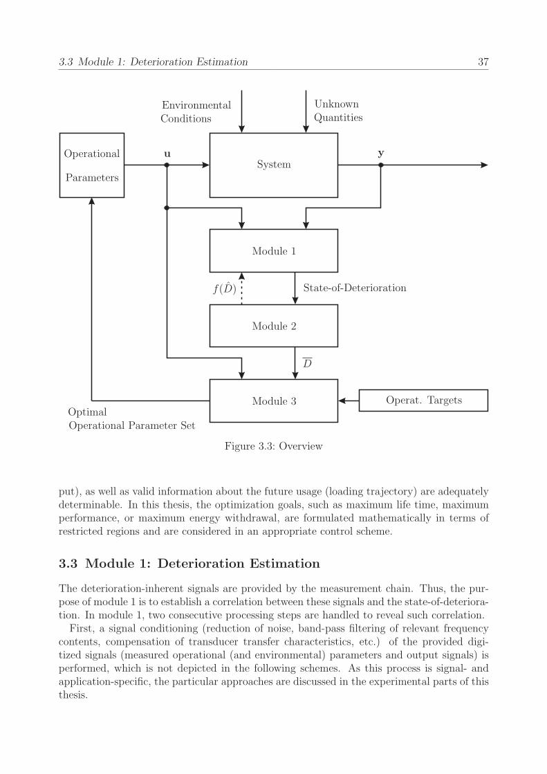
3.3 Module 1: Deterioration Estimation 37
Operational
ParametersSystem
u y
Module 1
Module 2
Module 3
f(D)
Operat. Targets
State-of-Deterioration
EnvironmentalConditions
UnknownQuantities
D
OptimalOperational Parameter Set
Figure 3.3: Overview
put), as well as valid information about the future usage (loading trajectory) are adequatelydeterminable. In this thesis, the optimization goals, such as maximum life time, maximumperformance, or maximum energy withdrawal, are formulated mathematically in terms ofrestricted regions and are considered in an appropriate control scheme.
3.3 Module 1: Deterioration Estimation
The deterioration-inherent signals are provided by the measurement chain. Thus, the pur-pose of module 1 is to establish a correlation between these signals and the state-of-deteriora-tion. In module 1, two consecutive processing steps are handled to reveal such correlation.First, a signal conditioning (reduction of noise, band-pass filtering of relevant frequency
contents, compensation of transducer transfer characteristics, etc.) of the provided digi-tized signals (measured operational (and environmental) parameters and output signals) isperformed, which is not depicted in the following schemes. As this process is signal- andapplication-specific, the particular approaches are discussed in the experimental parts of thisthesis.
3.3 Module 1: Deterioration Estimation 38
The more important second step in deterioration estimation is to convert the conditioned,deterioration-inherent signals into deterioration(-proportional) information by appropriatefilter (e. g., mathematical model). In dependency on the desired quality of output informa-tion (accuracy, performance, kind of output data, etc.), different theoretic modeling tech-niques are available. Due to the multitude of these techniques, only the general idea offilter selection and parameterization is introduced. The practical realizations are shownin Sections 4.3 and 5.3. The filter result is assumed in the following as a deterioration(-proportional) information. In dependency on the availability of (analytic and/or heuristic)knowledge, physical failure models, and/or observed deterioration symptoms of the system(process), appropriate (several sequential) filters are selected. A comprehensive overviewabout available filters (models) is given beforehand in Chapter 2, especially in Sections 2.4and 2.5.To validate the assumptions about the sequence and type of filters as well as the acquired
knowledge, baseline tests for comparable systems operated under comparable operations untilfailure are commonly performed. As operated under similar conditions, similar deteriorationdevelopments are expected. By taking only these information into account (immeasurableactual state-of-deterioration), the filter has to reveal the loading-deterioration connection,as depicted in Figure 3.5. If the real deterioration can additionally be measured at discretepoints k in system usage, a correlation between the measurements and the filtering resultreveals the accuracy of the combination and sequence of the chosen filters. This is ideais depicted in Figure 3.4. In dependency on the result, the filter have to be modified orexchanged to meet the measured deterioration level.As some faults and/or state-of-deterioration only become observable during transient oper-
ation (e. g., special maneuvers), the baseline test have to be designed such that deterioration-specific information are provided by the deterioration-inherent signals. By performing thebaseline tests at different states-of-deterioration, differences (proportional to the state-of-deterioration) are derived from the measured signals. These information are subsequentlyused to choose and adapt the filter.In general, filter results with negative deterioration tendency are implausible for non-
repairable systems as maintenance measures are not performed. Furthermore, neither self-healing effects nor faults due to sudden events (power shortage, etc.) are considered. Thelatter are commonly covered by redundancy countermeasures as described in Section 2.1.Hence, the filtering result is a monotonic increasing value over system usage as the deterio-ration is monotonic increasing.Depending on the possibility to estimate the actual state-of-deterioration (at discrete
instants of operation, etc.), one of the two following strategies is chosen.
Systems with Measurable State-of-DeteriorationFor systems with an assessable state-of-deteriorationD at discrete instants k of system usage,the assumed filter for continuous deterioration calculation is proved valid by the followingscheme, depicted in Figure 3.4.The estimated deterioration D, calculated by a filter, is compared to the measured dete-
rioration D. A measurable state-of-deterioration D can exemplary be the crack length of atensile test specimen, the thickness of an oxidation layer, etc.The deviation, calculated at instants k, between both is fed back to an algorithm, act-
ing as a controller known from classical control theory. In the ideal case, the deviation is
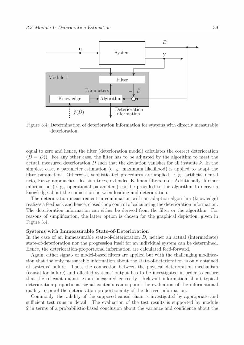
3.3 Module 1: Deterioration Estimation 39
uySystem
Filter
D
f(D)
D
Knowledge
Module 1
Parameters
DeteriorationInformation
Algorithm
−
Figure 3.4: Determination of deterioration information for systems with directly measurabledeterioration
equal to zero and hence, the filter (deterioration model) calculates the correct deterioration(D = D)). For any other case, the filter has to be adjusted by the algorithm to meet theactual, measured deterioration D such that the deviation vanishes for all instants k. In thesimplest case, a parameter estimation (e. g., maximum likelihood) is applied to adapt thefilter parameters. Otherwise, sophisticated procedures are applied, e. g., artificial neuralnets, Fuzzy approaches, decision trees, extended Kalman filters, etc. Additionally, furtherinformation (e. g., operational parameters) can be provided to the algorithm to derive aknowledge about the connection between loading and deterioration.The deterioration measurement in combination with an adaption algorithm (knowledge)
realizes a feedback and hence, closed-loop control of calculating the deterioration information.The deterioration information can either be derived from the filter or the algorithm. Forreasons of simplification, the latter option is chosen for the graphical depiction, given inFigure 3.4.
Systems with Immeasurable State-of-DeteriorationIn the case of an immeasurable state-of-deterioration D, neither an actual (intermediate)state-of-deterioration nor the progression itself for an individual system can be determined.Hence, the deterioration-proportional information are calculated feed-forward.Again, either signal- or model-based filters are applied but with the challenging modifica-
tion that the only measurable information about the state-of-deterioration is only obtainedat systems’ failure. Thus, the connection between the physical deterioration mechanism(causal for failure) and affected systems’ output has to be investigated in order to ensurethat the relevant quantities are measured correctly. Relevant information about typicaldeterioration-proportional signal contents can support the evaluation of the informationalquality to proof the deterioration-proportionality of the derived information.Commonly, the validity of the supposed causal chain is investigated by appropriate and
sufficient test runs in detail. The evaluation of the test results is supported by module2 in terms of a probabilistic-based conclusion about the variance and confidence about the

3.4 Module 2: Probabilistic-based Deterioration Model 40
u ySystem
FilterKnowledge
Module 1
f(D)
kfail
Deterioration-proportionalInformation
Figure 3.5: Determination of deterioration-proportional information for systems with im-measurable deterioration
derived deterioration-proportional information. If the validity is confirmed, the deteriorationis extracted from the measured quantities. Otherwise, the filter has to be exchanged ormodified in order to improve the information confidence.A consistent, reproducible correlation between the quantitatively derived information and
observed failures confirms the coherence between both. The result is that the deterioration-proportional information are calculated based on heuristic knowledge about the deterioratingphysical effects on the system and thus, on the measured signal.
3.4 Module 2: Probabilistic-based Deterioration Model
Based on an adequate deterioration(-proportional) information, module 2 realizes the taskof evaluating and ensuring the confidence of the proposed filter and determine the actualdeterioration phase. If the calculated deterioration can be correlated to the real deterioration(measurable state-of-deterioration), module 2 plays a minor role since the evaluation of theproposed model is realized within module 1 by adapting the deterioration-specific parame-ters. Here, module 2 mainly serves as a confidence check of the chosen filter and adaptionalgorithm for local and global operational conditions.For the estimation of a deterioration-proportional information, module 2 supports the
assumptions about the proposed/assumed connection between measured signal and derivedinformation to verify the chosen filter techniques and parameters. To compare the differ-ent progressions of the deterioration(-proportional) information with a sufficient degree ofconfidence, a sufficiently large data base (sample size of failed systems) has to be available.Since no correlation to the real deterioration is possible, the confidence check is realized bythe comparison of particular, scattering maximum values of the deterioration-proportionalinformation at failure of individual systems of one another.The influence of the stochastical concurrent events under constant operation (leading to
scattering instants of failure) have to be considered. Once a failure occurs, the individualmaximum tolerable deterioration is exceeded and a value for the maximum tolerated dete-rioration is obtained. The unification of these varying values is necessary to compare thesystems of one another. In the ideal case, many test with a large sample size of comparable
3.4 Module 2: Probabilistic-based Deterioration Model 41
systems can be performed and their individual failures can be measured. These informationabout the distribution of deterioration-proportional information over system usage will beconsidered and fed back to module 1. Assuming identical phase-specific, damaging effectsas well as identical accumulation, the accuracy of the calculation improves over the numberof failed systems.The scattering values for deterioration(-proportional) information at scattering instants
of experimentally observed failures is considered within a probabilistic-based approach.The probability distribution function is assumed as Weibull, which is a widely spread ap-proach [CFC06, GGQ, MZD03], etc. Furthermore, the Weibull analysis provides “reasonableaccurate failure analysis and failure forecast with extremely small samples” [Abe05]. Thediscrete information about the calculated deterioration(-proportional) information at theinstant of failure are the experimental basis for the estimation of an average deteriorationprogression.From statistics it is known that a sufficiently large sample size is required to state the
accuracy of the proposed distribution and its parameters. As fatigue tests, as these will beperformed in the subsequent chapters, are time- and cost-intensive, the following considera-tions reveal only an initial estimate of the Weibull parameters α and β due to a multitude ofuncertainties. Larger failure samples will detail and validate the first estimate. Nevertheless,the proposed parameters provide a base for the analysis of the propagation and influencingfactors on the fault propagation. Hence, the updated parameters (from further examinationsand observations) will slightly differ from the first approximation but will gradually stabilizeand approach the true Weibull distribution [Abe05].In [Wei51, GGQ], the estimation of the Weibull parameters from experiments is performed
for the Weibull function, given in Equation (2.8). Following [MXJ04], the Maximum Like-lihood Estimate (MLE) is used to reveal the parameters from experiment (complete data).The likelihood function is
L(α, β) =n∏
i=1
f(xi;α, β) , (3.1)
with f as the probability density function (here: Weibull) at each considered data pointxi for n systems (failures) and the unknown parameters of the chosen distribution. Theparameter estimation by MLE is performed numerically.The approach assumes that the dynamics of the Weibull parameters are slow with re-
spect to the deterioration. To prove the validity of the obtained parameters (goodness-of-fittest) typically methods are known in literature, e. g., the Chi-Square, Kolmogorov-Smirnoff,Anderson-Darling, and Nancy-Mann’s test. As introduced above, the validation requiresfurther failure samples and is hence, subject of comprehensive failure tests that are notdiscussed in this thesis.The Weibull distribution mainly serves as an approach to describe the average deteriora-
tion D within the considered phase. Additionally, the confidence interval (expressed by thestandard deviation) ensures the assumption and provides information about the applicabilityand accuracy of the proposed filter (module 1).Once an estimate for the Weibull parameters is obtained, the applicability of the assumed
distribution and numerically derived parameters is evaluated. Here, the standard deviationσ of the derived distribution is used as a measure of fit.

3.4 Module 2: Probabilistic-based Deterioration Model 42
kfail
D
Filter
Module 2
Deterioration(-proportional)Information
Figure 3.6: Module 2: Probabilistic-based evaluation of deterioration(-proportional) infor-mation
From Equation (2.4), the standard deviation
σ =
√√√√√+∞∫
−∞
(x− f(x)
)2
f(x)dx (3.2)
of the Weibull distribution is derived, describing the dispersion of the modal value f(x) (seeEquation (2.10)).The desired result is a small deviation from the modal. A sufficiently fit is obtained, if
all calculated, individual deterioration(-proportional) information vary less than σ from themodal deterioration D. This information, in terms of f(D), is fed back to module 1 inorder to falsify or verify the assumed filter and parameters. If proved valid, module 1 hasto be re-designed by an iterative, case- and application specific process to reach the bestfit. Otherwise, D represents the reference value for further estimations, i. e., trajectory ofthe modal deterioration D. This is especially important for comparing individual states-of-deterioration of different systems within the same deterioration phase with each other andthus, evaluating the initial deterioration of each system.In this thesis, a significant difference between failures due to different operational param-
eters is expected. Hence, module 2 considers varying operational parameters by particulardistributions. Each operational condition (in terms of parameters) reveal a distinct distri-bution. The general scheme of module 2 is given in Figure 3.6.Finally, module 2 realizes the determination of the actual deterioration phase (run-in,
permanent wear, or wear-out). This information is especially important for systems thatsuffer differently from certain maneuvers during different deterioration phases. The effect isthat certain maneuvers must not be performed during a particular phase as the impact ondeterioration is disproportional high than during other phases. As the amount, duration,relevance, etc. of each phase vary significantly from application to application, genericaspects of phase determination are given here. One indicator for a phase change can be achange in distribution parameters and can thus, be directly correlated to the parameters ofthe Weibull distribution. Beside that, the slope of deterioration can significantly change,e. g., from slow slope to high slope or vice versa. This effect is observed for the tribologicalsystem, discussed in Chapter 4.4.The application of the proposed module is illustrated in the following by a numerical
example. The deterioration is assumed to be depended on the chosen operational parameter

3.4 Module 2: Probabilistic-based Deterioration Model 43Modal
Deterioration
(-Proportion
al)Inform
ationD
System UsageEnd of Run-in Phase
Run-in Permanent Wear Wear-out
0
0
pset,1
pset,2
Figure 3.7: Simulated deterioration progression for comparable systems, operated under twodifferent operational parameters
set pset, and the individual behavior of the system. The parameter set consists of r individualoperational parameters (u1, u2, etc.), which are independent among each other. Since thedeterioration behavior changes, different deterioration progressions are possibly obtained foreach constant operational parameter set and deterioration phase.A mathematical model, representing the modal deterioration behaviorD, is simulated with
one parameter set pset,1 until failure. The instance of failure is described by the calculatedmodal (average) deterioration(-proportional) information D1 over system usage until failure.The next deterioration test is performed with the identical model but different parameterset pset,2. Again, the damage trace D2 is calculated. Each set of parameters, which is keptconstant over the test procedure, leads to a failure (D1,2 = Dmax) of the system after acertain system usage. The result is depicted in Figure 3.7.The dotted line represents the deterioration progression due to pset,1, the continuous line
depicts the deterioration due to pset,2.According to the significant change in deterioration progression (change in deterioration
slope), the above mentioned phases are introduced and the particular deterioration behaviorsare classified accordingly. It is notable that the end of run-in phase is identical for bothconsidered, different operational parameter sets but the transition from permanent wear
3.5 Module 3: Deterioration Prognosis 44
phase to wear-out phase is not.The effect of the chosen set of operating parameters on the deterioration process thus
depends on the particular phase. As depicted in Figure 3.7, pset,2 is less damaging during run-in phase than pset,1. The contrary is valid for phase 2. Derived from the simulation results,the operation should be modified at the transition points between the distinct phases inorder to reduce the deterioration and hence, maximize the usable remaining life (in terms ofsystem usage). The operating parameters are chosen phase-specific to maximize the possiblesystem usage.Furthermore, the maximum values for the instant of failure in system usage and the
deterioration(-proportional) information vary significantly in dependency on the particularphase. This coincides with the demand of phase-specific, optimal operational parameters forreducing the deterioration. This fact is important for module 3, as this module modifies theoperational parameters such that an optimal system usage is reachable.Summing up, module 2 realizes the approximation of an average (modal) propagation D
by a confidence interval of σ for each particular deterioration phase and thus, supports theplausibility of the filter, chosen in module 1. Furthermore, the impact of different operationalparameters on the phase-specific deterioration is determined and support module 3 by deter-mine the deterioration-optimal operation. The evaluation of the deterioration(-proportional)information is realized by a Weibull distribution and relevant statistical characteristics whoseparameters α and β are derived from observation and an appropriate algorithm (MLE). Withan increasing number of usage-failure relations, the observed behavior ((assumed) deterio-ration progression) can be described more detailed. In conjunction with sufficiently largefailure samples, a validation of the proposed filter and its accuracy can be stated. Hence, astatistically ensured data base is developed that is subsequently used in module 3 to supportthe life time control algorithm.
3.5 Module 3: Deterioration Prognosis
The aim of life time control is the extension of a possible, deterioration-minimal usage of asystem to its maximum life time along with the fulfillment of the primary function at the sametime. The trivial solution (e. g., an immediate stop of the system/process at the occurrence ofa fault) of avoiding deterioration is obviated by defining appropriate limits for the consideredoperational parameters. Hence, the task is to identify the deterioration-sensitive/-decisiveoperational parameters, possibly for each deterioration phase. The requirement and possiblesolutions of determining these operating conditions is discussed in this module.In order to control the life time, the deterministic part of the deterioration process has
to be manipulated, which mainly depends on the chosen sets of operational parametersat particular wear phases. The stochastic events that do not depend on the operationalconditions, are covered by the probabilistic-based considerations in module 2. Therefore, theoperational parameters, governing the deterioration process, have to be adjusted situation-specific. The analysis of scattering input parameters on the system performance is essentialfor dependability evaluation.Once the adjustable parameters and limits are determined, the condition-based set of
parameters has to be chosen, e. g., from a data base. The parameter sets need to encompassall applicable field conditions to ensure a sufficiently high confidence in reliability estimates
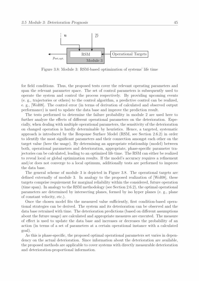
3.5 Module 3: Deterioration Prognosis 45
D
Module 3
RSM Operational Targets
u
pset,opt.
Figure 3.8: Module 3: RSM-based optimization of systems’ life time
for field conditions. Thus, the proposed tests cover the relevant operating parameters andspan the relevant parameter space. The set of control parameters is subsequently used tooperate the system and control the process respectively. By providing upcoming events(e. g., trajectories or others) to the control algorithm, a predictive control can be realized,e. g., [Wol08]. The control error (in terms of derivation of calculated and observed outputperformance) is used to update the data base and improve the prediction result.The tests performed to determine the failure probability in module 2 are used here to
further analyze the effects of different operational parameters on the deterioration. Espe-cially, when dealing with multiple operational parameters, the sensitivity of the deteriorationon changed operation is hardly determinable by heuristics. Hence, a targeted, systematicapproach is introduced by the Response Surface Model (RSM, see Section 2.6.2) in orderto identify the most significant parameters and their connection amongst each other on thetarget value (here the usage). By determining an appropriate relationship (model) betweenboth, operational parameters and deterioration, appropriate, phase-specific parameter tra-jectories can be calculated, leading to an optimized life time. The RSM can either be realizedto reveal local or global optimization results. If the model’s accuracy requires a refinementand/or does not converge to a local optimum, additionally tests are performed to improvethe data base.The general scheme of module 3 is depicted in Figure 3.8. The operational targets are
defined externally of module 3. In analogy to the proposed realization of [Wol08], thesetargets comprise requirement for marginal reliability within the considered, future operation(time span). In analogy to the RSM methodology (see Section 2.6.2), the optimal operationalparameters are determined by intersecting planes, formed by iso hyper planes (e. g., planeof constant velocity, etc.).Once the chosen model fits the measured value sufficiently, first condition-based opera-
tional strategies can be derived. The system and its deterioration can be observed and thedata base retrained with time. The deterioration predictions (based on different assumptionsabout the future usage) are calculated and appropriate measures are executed. The measureof effect is used to update the data base and increases or decreases the probability of anaction (in terms of a set of parameters at a certain operational instance with a calculatedgoal).As this is phase-specific, the proposed optimal operational parameters set varies in depen-
dency on the actual deterioration. Since information about the deterioration are available,the proposed methods are applicable to cover systems with directly measurable deteriorationand deterioration-proportional information.

3.5 Module 3: Deterioration Prognosis 46
System
Usage
[%]
0texttexttextOperational Parameter 2u2,ll
u2,ul
Operational Param
eter 1texttextex
t
u1,ll
u1,ul
100
Figure 3.9: Simulation results for maximum system usage over two-dimensional operationalparameter space
This module forms thus the missing link between classical structural health monitoring(SHM) approaches and structural health control (SRCE-concept) in order to realize thedeterioration-depended control of the life timeThe simulation example, introduced in module 2, is carried on in order to demonstrate
the general idea.The results are depicted in Figure 3.9. The upper and lower limits for each operating pa-
rameter must be determined and provided to the algorithm. Here, the individual limitationsare denoted by ur,ll for the lower limit and ur,ul for the upper limit, respectively.As shown, both parameters are varied within their specified limits. The resulting plane
represents the maximum value D for system usage at point of failure. The informationobtained by these (simulated) failure test is the optimal region for a constant parameter set.Referring to Figure 3.7, the constant set of operating parameters pset,2 leads to the maximumpossible system usage. As depicted, the usage could be extended if the operation is changedwhen entering the permanent wear phase. During the run-in phase the different extendof damage can be determined detailed. Again, interpolating planes using the measuredvalues as supporting points can help to point out the optimal set of operating conditionfor this phase. In the 2D space (only two independent parameters, r = 2), this is realizedgraphically. Once the system has more operational parameters r > 3, this method can
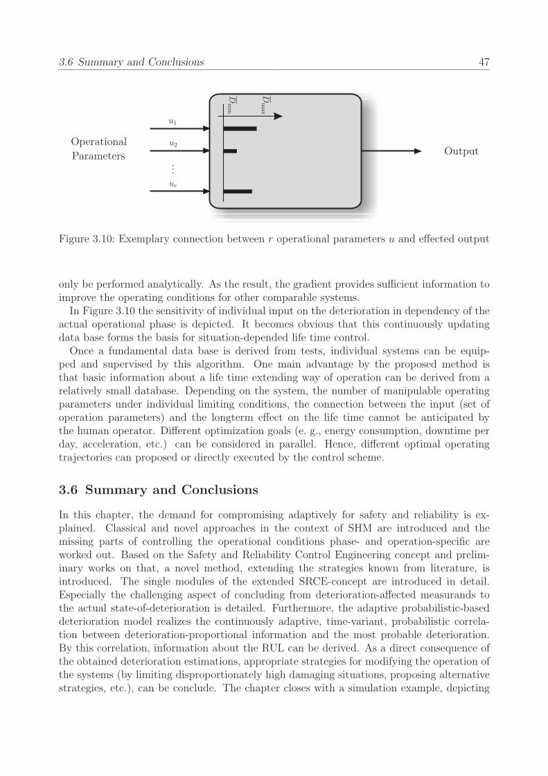
3.6 Summary and Conclusions 47
u1
u2
ur
Dmax
Dmin
OutputOperational
Parameters...
Figure 3.10: Exemplary connection between r operational parameters u and effected output
only be performed analytically. As the result, the gradient provides sufficient information toimprove the operating conditions for other comparable systems.In Figure 3.10 the sensitivity of individual input on the deterioration in dependency of the
actual operational phase is depicted. It becomes obvious that this continuously updatingdata base forms the basis for situation-depended life time control.Once a fundamental data base is derived from tests, individual systems can be equip-
ped and supervised by this algorithm. One main advantage by the proposed method isthat basic information about a life time extending way of operation can be derived from arelatively small database. Depending on the system, the number of manipulable operatingparameters under individual limiting conditions, the connection between the input (set ofoperation parameters) and the longterm effect on the life time cannot be anticipated bythe human operator. Different optimization goals (e. g., energy consumption, downtime perday, acceleration, etc.) can be considered in parallel. Hence, different optimal operatingtrajectories can proposed or directly executed by the control scheme.
3.6 Summary and Conclusions
In this chapter, the demand for compromising adaptively for safety and reliability is ex-plained. Classical and novel approaches in the context of SHM are introduced and themissing parts of controlling the operational conditions phase- and operation-specific areworked out. Based on the Safety and Reliability Control Engineering concept and prelim-inary works on that, a novel method, extending the strategies known from literature, isintroduced. The single modules of the extended SRCE-concept are introduced in detail.Especially the challenging aspect of concluding from deterioration-affected measurands tothe actual state-of-deterioration is detailed. Furthermore, the adaptive probabilistic-baseddeterioration model realizes the continuously adaptive, time-variant, probabilistic correla-tion between deterioration-proportional information and the most probable deterioration.By this correlation, information about the RUL can be derived. As a direct consequence ofthe obtained deterioration estimations, appropriate strategies for modifying the operation ofthe systems (by limiting disproportionately high damaging situations, proposing alternativestrategies, etc.), can be conclude. The chapter closes with a simulation example, depicting

3.6 Summary and Conclusions 48
the numerical applicability and potential of the proposed framework.Finally, the progression of the deterioration(-proportional) information and the probabilis-
tic evaluation have to be carried out for varying operation parameters. A similar idea hasbeen investigated in [NF99]. There, the influence of variable operating conditions on theexpected service life was evaluated by a multi-modal Weibull distribution. It is shown thatsimilar results for the distribution parameters are obtained, whether constant or variableoperation is observed.

4 Application to Tribological System
The modular concept from Chapter 3 is explained in detail by giving the example of a me-chanical system, which suffers from wear effects induced by operating conditions, local ma-terial defects, etc. To gain the relevant information about the actual state-of-deterioration,the measured signals are filtered and correlated with meaningful baselines. Hence, a roughclassification of relevant signals (signal contents, frequency range, etc.) can be stated. Fur-thermore, the connection between applied loading and resulting deterioration can be exper-imentally derived from observations and used in combination with a mathematical model topredict the remaining life time.In order to reach these ambitious goals for an industrial machine, the process of dete-
rioration is investigated in detail to determine the relevant physical failure mechanisms.Subsequently, a novel, specialized measurement chain is developed that is especially sensi-tive to the deterioration-relevant quantities. In conjunction with the material investigationsand application-specific measurement concept, filters are designed in order to derive thedeterioration-proportional information. The obtained results of different operation-to-failuretests are consolidated and evaluated by probabilistic considerations. In addition to the novelmeasurement chain and filters, optimized operational parameters are proposed for the firsttime, paving the way for an optimized, wear-reduced operation of the tribological system.
4.1 Motivation
In the following, the typical failure of a mechanical (tribological) system is considered. Gen-erally speaking, tribology is a sciences dealing with surfaces that interact which each otherdue to relative movements [GfT]. It covers the complete field of friction and wear, includinglubrication and interactions between boundary surfaces. In tribology, wear is defined as thecontinuing deterioration of a solid surface, caused by mechanical stress, e. g., contact andrelative motion of a rigid counter body. It generally involves progressive loss of material. Atribological system contains all material components and their (variable) characteristics dueto operation.As an application example of a system suffering from wear, an industrial scrap bailing
press is considered. This specific machine is mainly employed in the automotive industry,especially in car body plants. The scrap material (aluminum, steel, etc.), resulting from diecutting processes, is fed to the press and subsequently compacted into bales by hydrauliccylinders.The linear compression movements of the hydraulic cylinders are guided by wear plates.
The guidance is realized by a structural shape (corrugated washboard profile) of the wearplates. The tribological effects at the wear plate’s surface are reduced by special materials(e. g., special blooming) in combination with automated lubrication systems. Anyhow, themain reason for failure is the occurrence of plate jams caused by an excessive surface wear-out.The current (preventive) maintenance strategies focus on an avoidance of wear-out failure bychanging the wear plates in (constant) maintenance intervals. Hence, the on-line monitoring

4.1 Motivation 50
of the wear plate’s surfaces is necessary to optimize the system’s reliability by conditionbased maintenance. The aim is to equip the machine with sensors in sheltered positions thatprovide deterioration-inherent signals to a wear monitoring and control system.In order to develop a reasonable measurement chain and operational strategies, all relevant
information about the considered system and its typical failure are evaluated. Therefor, wearplates from field failure are examined and typical effects are discussed in Section 4.1.1.Based on this knowledge, a developed test rig, realizing the operational conditions, is
briefly introduced in Section 4.1.2. Subsequently, the wear plates failures, produced by thetest rig, are analyzed and the results are compared with the field failures. By showing thatthe wear plates fail due to identical deterioration mechanisms, the applicability of the testrig for failure examinations is proven.Due to the complexity of the wear process (locally and timely distributed, stochastically
occurring incremental deterioration), a signal-based approach for deterioration evaluation ischosen. As the physical failure mechanisms are investigated in detail, a direct correlationbetween abraded material (wear) and emitted acoustic emission (AE) is found to describequantitatively and qualitatively the deterioration process. Therefore, adequate sensing tech-nologies are introduced in Section 4.2 to sense these effects. Under the consideration ofapplicability and sensitivity to deterioration-indicating signals (tribological effects), an ade-quate measurement chain for acoustic emission detection is developed and applied.As module 1 is developed in close conjunction with the AE measurement chain, appropriate
filters are introduced in Section 4.3 that realize the extraction of deterioration-proportionalinformation. The revealed information are correlated with classical process information tovisualize abnormal behavior (stochastically occurring AE events). As the (progression of)deterioration is immeasurable, this correlation is especially important to identify and validatethe assumed filter characteristics and chosen parameters. The proposed filter results reveal arelation between measured AE energy and observed instant of failure and is hence assumedto be appropriate to describe the incremental deterioration.As expected, the operation reveal a stochastic life time distribution of comparable systems,
operated under comparable operating conditions. Hence, module 2 (Section 4.4) details theidea to extract typical deterioration indicators over system usage to evaluate at an earlystage an individual system with its individual deterioration behavior. It will be shownthat the deterioration behavior is clearly divided into three distinct deterioration phaseswhich are considered separately. Hence, module 2 evaluates the deterioration-proportionalinformation of a supervised system during operation and correlates its individual behaviorto history data. Based on this heuristic knowledge, the estimation of the most probabledeterioration propagation is realized.As proposed beforehand, the information about the RUL is an important quantity for
maintenance strategies. The even more valuable information is, how to extend the currentRUL by adapting the operation parameters adequately. The knowledge about the relationbetween the operational conditions (speed of cylinder movement, lubrication, etc.) and theinstant of failure (correlating with the propagation of the deterioration-proportional infor-mation) is proposed to be the key information for adaptive, reliability-centered operation.It will be shown that the quality of the wear plates predetermines the maximum life time ofthe system. A targeted adaption of operational parameters is not sufficient to significantlyinfluence the RUL. This will be illustrated based on the deterioration progression duringrun-in phase.

4.1 Motivation 51
4.1.1 Field Failure
In [Bes05], a typical field failure of a wear plate is examined by hardness measurements,light optical microscope, Energy Dispersive X-ray (EDX), and Scanning Electron Microscope(SEM) analysis. Different probes from different positions in the wear plates were taken andanalyzed by the above mentioned techniques. Three different wear mechanisms (terminologyaccording to [CH10, BB10]) were identified: adhesive wear (cold-welding, scuffing), abrasivewear (scouring abrasion), and surface fatigue (crack growth). Those mechanisms are typicalfor systems under reciprocating slide wear, e. g., described in [FK01, FLK+03].Based on these examinations, [Bes05] proposes the following causal chain of wear: during
the compression movement of the cylinder, bulk material from the wear plates is abradedof the surfaces. These hard and sharp debris (acicular martensite) gets strain-hardenedand roughens the surfaces (scuffing, scouring abrasion, fretting). Subsequently, the weardebris (and other debris from crap material, e. g., thin pieces of metal and off cuts) gallsagain at different places. Insufficient lubrication with high (local) temperatures increasesthe wear-out rate even more. This procedure of break out and galling occurs alternately andconcurrently. The washboard profile is deformed significantly and leads at some point to thefailure, observed as a plate jam. In parallel to the conclusion of [Bes05], [FLK+03] proclaimsthat wear under fretting load is the result of debris formation and ejection.Hence, the failure results from extensive, stochastically occurring material changes, i. e.,
scouring abrasion, debris, and galling. The time instant of failure is thus depended on theabrasive debris (size, amount) and disadvantageous aggregation and ejection.
4.1.2 Test Rig
To examine the factors driving the material changes, a test rig is used and extended byadditional sensors.The relevant parts of the test rig are shown in Figure 4.1. The dimensions of all components
are chosen in order to meet the field application and hence the operation conditions. The tri-bological system consists of two wear plates, the body locked into position, the counter bodyconnected to the cylinder. An electro-mechanical valve, controlling the hydraulic cylinder,realizes the linear, reciprocating movement of the body. The horizontal movement is limitedto a linear movement by the washboard profile of the wear plates. The vertical movementis prevented by an adjustable contact pressure, realized by a pneumatic cylinder and a leverarm (double T beam). An automated lubrication with field lubricant at fixed time intervalsis also realized. Typical measurements from field application (normal force, acceleration,hydraulic pressure, temperature, etc.) are recorded by the real-time system (not depicted).The valve and hence the cylinder movement are controlled such that the relevant parameters(stroke velocity, ratio between operation and idle mode, etc.) are represented. In analogy tofield operation, the counter body strokes over a distance of 1.6m within 40s and subsequentlypauses for 70s (idle mode). This cycle of 110s is repeated steadily.The test rig validation was performed by operating the test rig under application-relevant
conditions. The failures produced by the test rig were examined and compared to thefailures observed in field usage (see Section 4.1.1). According to [Bes07], the types of wear,the progress of damage, surface temperatures, thickness of accumulated material (by cold-welding, etc.) were identical, i. e., the test rig is applicable to reproduce application-relevant

4.1 Motivation 52
Figure 4.1: Test rig for wear examinations
conditions and hence field failure sufficiently accurate.Various short- and long-term tests were performed to realize different damage progressions
by varying the operational conditions. More specifically, the type of lubricant, the lubricationintervals, the hydraulic pressure (and hence the stroke velocity), the ratio between operationand idle mode, etc. were modified in a targeted manner. The worn out plates were analyzedand the results are discussed in detail, e. g., in [DS09, HDS10, RDS10, Rav11].In Figure 4.2(a), the bulk material (acicular martensite) of a wear plate before operation
is depicted. During operation and until fault, the material structure is changed by e. g.,loading. A typical profile of a worn out plate is shown in Figure 4.2(b). Beside the bulkmaterial (lower section of figure), different layers with deviating grain structures are present.Those layers consists of cold welded abraded bulk material and lubricant. The cavities(material defects) are starting points for micro and macro cracks that reduce the mechanicalstrength. When propagating through the material, the cold welded debris can abrade again.As discussed in [KRC+10], martensite needles form microstructural barriers which preventa crack propagation. In contrary to this assumption, martensite needles are assumed toprovide a preferred crack propagation direction (along phase interfaces).As stated and illustrated above, the test rig reproduces field failure. Hence, the test rig
is used to obtain deterioration-relevant information for fatigue life time examinations interms of baselines. Furthermore, specially designed experiments are used to examine thedeterioration behavior under various operation conditions.

4.1 Motivation 53
10µm
(a) Bulk material of unused wear plate
10µm
(b) Worn out plate; cold-welding, micro cracks,and bulk material
Figure 4.2: SEM results for wear plates
As the primer effect leading to failure is known and reproducible by the test rig, henceforthappropriate measurement techniques have to be evaluated to reveal unambiguous informationabout deterioration.
4.1.3 Acoustic Emission due to Material Change
As described in Section 4.1.2, the failure appears as a result of excessive material changes(scuffing, cold-welding). Especially abrasion is identified as the primary cause of deteriora-tion and hence, failure. During the various examinations of worn out plates, the positionof abrasion and subsequent cold-welding was stochastically distributed over the plate sur-face. Therefore, the deterioration is a highly stochastically process which depends on theoperational conditions and initial plate damage and has to be supervised continuously byappropriate techniques.A multiplicity of research has been done in literature on the effect of abrasion in metallic
material and its detection. Especially the detection of acoustic emissions turned out to bepromising in the context of structural health monitoring. In general, acoustic emission isdefined as “the class of phenomena whereby transient elastic waves are generated by therapid release of energy from localizes sources within a material”, [AST90, DIN EN 1330].In [Hol82] is stated that the “formation and propagation of micro cracks are associated
with the release of energy.” This energy (shock wave) propagates through the material andmoves to its surface. In [Poh03], micro-structural deformations of material are detected bymeasuring the emitted acoustic emission during deformation. These emissions offer a greatpotential for non-destructive analysis of deterioration and supervision.In [BMS90], acoustic emission analysis is used to differentiate between different wear mech-
anisms occurring in dry and lubricated sliding metallic contacts. The test conditions indicatea direct empirical relationship between the AE signal and the wear volume removed (abra-sion). Further research show that “the time-dependent nature of the acoustic signal is able

4.2 Acoustic Emission Measurement 54
to detect the presence of wear-reducing additives and the predominant wear process occur-ring” [BM91]. Hence, the correct (wear-depended) lubricant is essential for wear-minimaloperation. It is stated that “acoustic emission signals increase with alumina particle con-centration added to the lubricant.” Hence, the acoustic emission also depends on the type(quantity) of (wear) debris.The evaluation of AE events are a “possibility for continuously monitoring wear and
for basic studies of the wear process”, as these signal arise from fundamental wear pro-cesses [HK91]. Again, a dependency of acoustic emission activity and wear rate is measuredin sliding metallic contacts. It is shown by experiments that “changes in acoustic emissioncount rates correspond to changing wear rate.”In [LYY93], material change is described as the “deformation processes in solids, such
as dislocation movements, crack propagation [...] (that) produce stress waves at ultrasonicfrequencies [...].” Experimental test with metallic specimens in relative sliding motion areperformed and “clear indications that AE is intimately related to the fundamental materialand surface actions in the wear zone” are found. The measured acoustic emissions (predom-inant frequencies) are finally assigned to the severity of deformations and wear conditions.As stated by [MvKM05], “acoustic emission is a non-destructive method that is sensitive
to mechanical waves created in many materials by sudden displacements due to microscopicstress release.” Acoustic emission is not limited to deformation processes in metals but is alsowildly used in general structural health monitoring domains, e. g., carbon fiber componentsin aeronautics, etc.A crack, as a common appearance of a defect, is considered in [BFG06] as a typical
source of AE. Such burst signals are attributed to plastic deformations in metallic materials.Subsequently, SHM-related examinations are discussed for composite materials with the goalof residual life time prediction.Finally, in [BBHF07] the applicability of AE measurements for deterioration estimation is
discussed. It is stated that a change in measurement of AE on the same structure at differenttimes is related with a change in material. These changes “yields indications of defect accu-mulation or growth when keeping all other test parameters (e. g., emitter efficiency, receiversensitivity, and coupling) constant.” In conclusion, acoustic emission signals, especially inultrasonic frequency range, contain deterioration-equivalent information.
4.2 Acoustic Emission Measurement
The goal is to identify a relation between the obtained stochastically, transient occurringemissions (due to material changes) and the deterioration to reveal a unique connectionbetween both. Therefore, the three elements (see Figure fig:GenMeasChain) of the novel,problem-specific measurement chain are introduced in the following to realize the in-situmeasurements. Furthermore, these measurements are integrated into the test rig control toenable correlations to existing process information, e. g., chamber pressures of the cylinder,position and acceleration of the piston, body temperature, compressive force, etc.
4.2.1 Transducer
The measurement of material changes by acoustic emission detection is a promising butalso a challenging task. The stress waves at ultrasonic frequencies, generated by material

4.2 Acoustic Emission Measurement 55
changes, propagate through the structure and meet the (plate) surface. To measure thesepotentially very small and short-time surface displacements without any coloration or un-wanted side effects, a no-contact measurement (e. g., laser interferometer) would be best.Due to low robustness of these systems, surface-bonded transducers with high sensitivity andwide bandwidth have eo be chosen. According to [Shu02], a transducer with piezoelectricproperties is best suited for this purpose.The direct piezoelectric effect relates the (rapidly changing) mechanical load (surface dis-
placement due to shock wave) to a changing voltage on the insulated electrodes of thepiezoelectric element. The piezoelectric voltage should be measured reactionless to avoidany shifting effects like attenuation, amplification, phase shift, etc. The physical effects ofpiezoelectric materials are described in detail, e. g., in [Fra10, MvKM05, TEKP10, JBS+04].Derived from thermodynamics, the energy conversion (piezoelectric effect) is analytically
described by
D3 = d33T + ǫT33E (4.1)
as a linearly coupling of two different effects, namely electricity and mechanics [Ike90]. Theequation (4.1) describes the relation between the mechanical stress T , the electric field E ,and the electrical flux density D.The constants d, and ǫ describe the piezoelectric constant, and the dielectric permittivity,
respectively. The superscript T denotes that the parameter is obtained at constant (zero)stress T and is hanec a consant. For frequency-dependent investigations, the permittivity isused instead. The subscript 3 denote the direction of the stress axis, the index 33 that thepolarization axis is parallel to the stress axis.According to [Ike90], the electric current I is calculated from equation (4.1) by integrating
the electric field
I = jω
∫
x1,x2
D dx1 dx2 , (4.2)
with x1 and x2 both perpendicular to the stress axis S and equal to the diameter d⊘ of thechosen ceramic.The formula for the current I, induced by the direct piezoelectric effect, yields
I = jω[d33F + ǫT33d⊘U
], (4.3)
with I as the electric current, F as the applied force, and U as the voltage.All values are varying with the frequency ω of the input F . Hence, the frequency-
dependency of the permittivity ǫ is considered by replacing ǫ by the admittance Y of thepiezoelectric element.Additionally, [Ike90] proposes a constant φ to summarize the material constants, coupling
condition, etc. By operating the transducer in open circuit condition (I = 0), the transferbehavior of a piezoelectric material as a sensor is
U = −Zφv , (4.4)
with Z as the impedance, v as the velocity of surface movement, and Zφ as the governingfactor of the dynamics. It is important to notice that any movement (and hence velocity v),perpendicular to the direction of plate movement, generates a voltage U .

4.2 Acoustic Emission Measurement 56
Material type PIC 255
Curie-Temperature Tc = 350CPiezoelectric charge constant d33 = 400e−12 C/NFrequency constant
Nt = 2000Hzmof thickness oscillation
GeometryDiameter d⊘ = 10mmThickness TH = 0.55mm
Table 4.1: Data of piezoelectric material PIC255 [PI11]
Amongst a variety of piezoelectric materials, a non-resonant broadband, lead-zirconium-titanate (PZT) ceramic in disc shape with metal silver electrodes and wrapped contacts ischosen. The important geometric dimensions and directional material property for thicknessoscillations of plates are given in Table 4.1.The serial resonance frequency for the chosen PIC 255 material is
fs =Nt
TH= 3.6MHz . (4.5)
In the frequency range less than 3.6MHz, this unbonded ceramic provides an electri-cal impedance response Z as shown in Figure 4.3. The expected capacitative behavior isobserved. The frequency response measurement was performed on a Network Analyzer ac-cording to [DIN 50321-1] and validated with OEM measurements.To guarantee a minimum attenuation of the emitted acoustic signals, the transducer has
to be attached as close as possible to the wear zone. Therefore, the transducer is bondedto the backside of the moving wear plate. The requirements for the attachment are: goodmechanical coupling, low (frequency-depended) attenuation of couplant, reproducibility, andelectrical insulation.The couplant between the ceramic surface and the wear plate is required to reduce the
acoustic impedance mismatch (reflection coefficient) and guarantee an electric insulation.The latter is realized by a polyvinyl chloride (PVC) layer between the ceramic and the metalsurface (surface resistivity of PVC > 1013Ω). The layer needs to be very thin (here: approx.20µm, see Figure 4.5) to avoid an acoustical insulation and hence signal attenuation. Thesame holds true for the glue layers. To attach both, the insulating layer to the metal and theceramic to the insulating layer, a cyanoacrylate glue is used; the adherents are free of grease,dust, and adhesives. The glue cures at room temperature to avoid artificially aging of thematerial as described in [BBHF07]. The aging of the piezoelectric material, as it mainly refersto reduction in remnant polarization due to service loads, environmental exposure, etc., isnot relevant for the considered short-term experiments and hence neglected [BBHF07]. Onlyduring soldering of the contacts, the effect of aging is considered by keeping the solderingtemperature below TC
2. To reduce reflections of the acoustic emissions on the surface, the
nominal surface roughness is reduced by grinding with sandpaper P1200 (grain size accordingto [DIN 6344]).The schematic application of the ceramic, insulating layers and wear plate is depicted in
Figure 4.4.
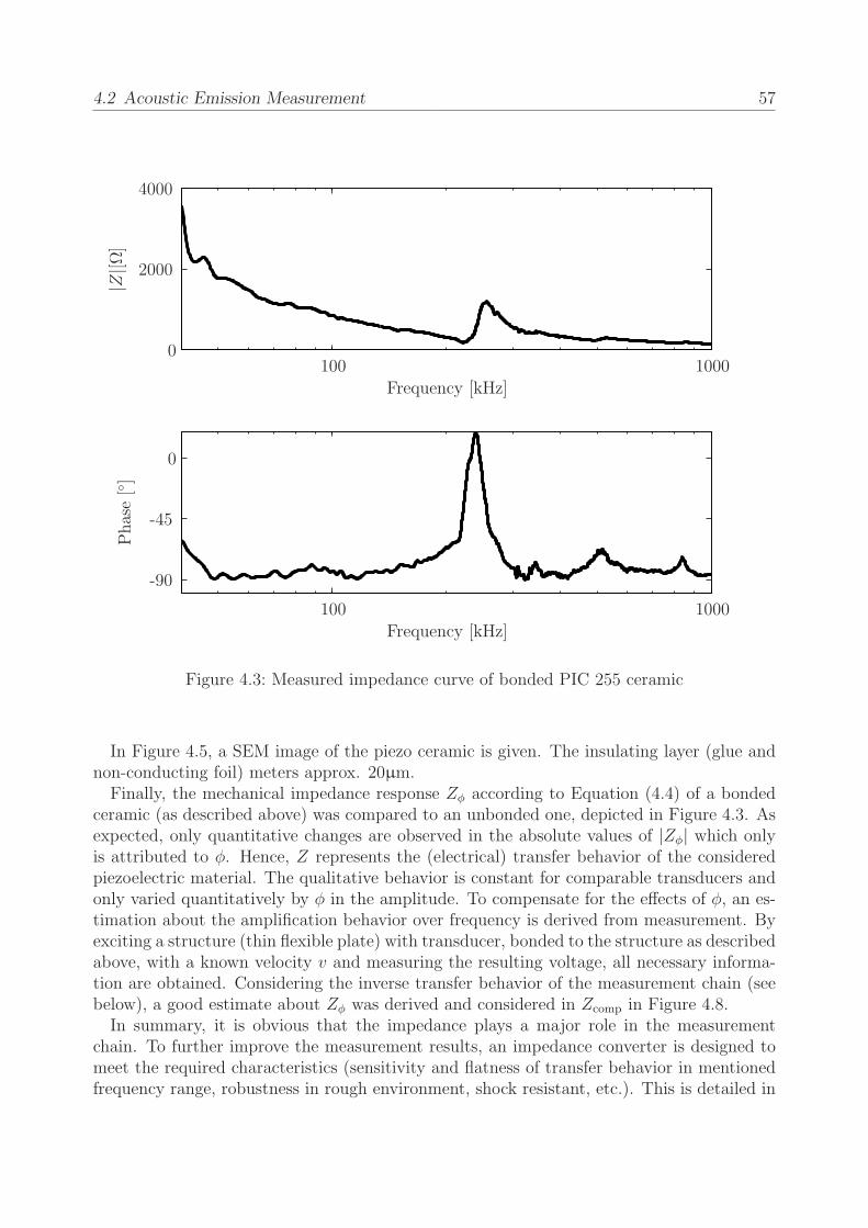
4.2 Acoustic Emission Measurement 57
Phase[]
Frequency [kHz]
Frequency [kHz]
|Z|[Ω
]
0
0
-45
-90
100
100
1000
1000
2000
4000
Figure 4.3: Measured impedance curve of bonded PIC 255 ceramic
In Figure 4.5, a SEM image of the piezo ceramic is given. The insulating layer (glue andnon-conducting foil) meters approx. 20µm.Finally, the mechanical impedance response Zφ according to Equation (4.4) of a bonded
ceramic (as described above) was compared to an unbonded one, depicted in Figure 4.3. Asexpected, only quantitative changes are observed in the absolute values of |Zφ| which onlyis attributed to φ. Hence, Z represents the (electrical) transfer behavior of the consideredpiezoelectric material. The qualitative behavior is constant for comparable transducers andonly varied quantitatively by φ in the amplitude. To compensate for the effects of φ, an es-timation about the amplification behavior over frequency is derived from measurement. Byexciting a structure (thin flexible plate) with transducer, bonded to the structure as describedabove, with a known velocity v and measuring the resulting voltage, all necessary informa-tion are obtained. Considering the inverse transfer behavior of the measurement chain (seebelow), a good estimate about Zφ was derived and considered in Zcomp in Figure 4.8.In summary, it is obvious that the impedance plays a major role in the measurement
chain. To further improve the measurement results, an impedance converter is designed tomeet the required characteristics (sensitivity and flatness of transfer behavior in mentionedfrequency range, robustness in rough environment, shock resistant, etc.). This is detailed in
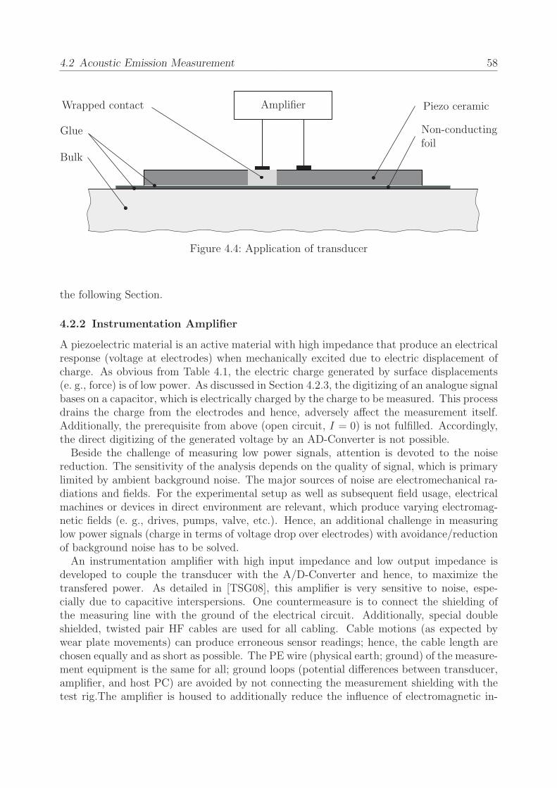
4.2 Acoustic Emission Measurement 58
Glue
Bulk
Piezo ceramic
Non-conductingfoil
AmplifierWrapped contact
Figure 4.4: Application of transducer
the following Section.
4.2.2 Instrumentation Amplifier
A piezoelectric material is an active material with high impedance that produce an electricalresponse (voltage at electrodes) when mechanically excited due to electric displacement ofcharge. As obvious from Table 4.1, the electric charge generated by surface displacements(e. g., force) is of low power. As discussed in Section 4.2.3, the digitizing of an analogue signalbases on a capacitor, which is electrically charged by the charge to be measured. This processdrains the charge from the electrodes and hence, adversely affect the measurement itself.Additionally, the prerequisite from above (open circuit, I = 0) is not fulfilled. Accordingly,the direct digitizing of the generated voltage by an AD-Converter is not possible.Beside the challenge of measuring low power signals, attention is devoted to the noise
reduction. The sensitivity of the analysis depends on the quality of signal, which is primarylimited by ambient background noise. The major sources of noise are electromechanical ra-diations and fields. For the experimental setup as well as subsequent field usage, electricalmachines or devices in direct environment are relevant, which produce varying electromag-netic fields (e. g., drives, pumps, valve, etc.). Hence, an additional challenge in measuringlow power signals (charge in terms of voltage drop over electrodes) with avoidance/reductionof background noise has to be solved.An instrumentation amplifier with high input impedance and low output impedance is
developed to couple the transducer with the A/D-Converter and hence, to maximize thetransfered power. As detailed in [TSG08], this amplifier is very sensitive to noise, espe-cially due to capacitive interspersions. One countermeasure is to connect the shielding ofthe measuring line with the ground of the electrical circuit. Additionally, special doubleshielded, twisted pair HF cables are used for all cabling. Cable motions (as expected bywear plate movements) can produce erroneous sensor readings; hence, the cable length arechosen equally and as short as possible. The PE wire (physical earth; ground) of the measure-ment equipment is the same for all; ground loops (potential differences between transducer,amplifier, and host PC) are avoided by not connecting the measurement shielding with thetest rig.The amplifier is housed to additionally reduce the influence of electromagnetic in-

4.2 Acoustic Emission Measurement 59
1µm200µm
Figure 4.5: SEM image of applied transducer; detail: zirconium titanate structure
terspersions from valves, etc. Finally, the amplifier is located as close as possible to thetransducer [MvKM05].The amplifier itself is independently powered by batteries and hence, no ripple voltages
are induced by the power supply. Additionally, no ground loop is induced by an externalpower supply in the enclosed housing. Finally, the output of the amplifier is electricallyresilient and can drive the downstream A/D-Converter (see Section 4.2.3).In Table 4.2, the input characteristics of the subsequent A/D-Converter are given. For
the design of the output characteristic of the instrumentation amplifier the valid measuringrange is important. In preliminary tests, piezoelectric voltage up to ±3V were recorded.Hence, a balanced potential divider is necessary to avoid damage to the AD-Converter.The electrical connection diagram of the amplifier with integrated balanced potential di-
vider circuit is depicted in Figure 4.6.The balanced potential divider is designed such that the ratio can be varied by DIP
switches from 1:1 to 4:1 conversion. Accordingly, the output of the amplifier can be adjustedto special applications to match the maximum input ratings of the resilient A/D-Converter.The impedance of the measurement chain (connecting cable with impedance converter
with balanced potential divider at voltage division 2:1) without the transducer is shown inFigure 4.7.This characteristic is assumed be time invariant and hence considered during signal anal-
ysis as a constant transfer behavior.

4.2 Acoustic Emission Measurement 60
DIP SW1DIP SW2
DIP SW3DIP SW4
100kΩ100kΩ
100kΩ100kΩ
1kΩ
1kΩ
0...3kΩ
0...3kΩ
100µF
100µF
100nF
100nF
3V
3V
BNC
BNC
TW
INAX
AD8137
12345 6 7 8
Figure 4.6: Electrical circuit of impedance converter and balanced potential divider
The success of these countermeasures to noise was evaluated by various test scenarios.The comparison between measurements without and with the above mentioned actions isperformed by frequency investigations.
4.2.3 A/D-Converter
The last step in the measurement chain is the digitizing of the analogue signal. In general,an A/D-Converter (ADC) quantized an analogue signal into a time and value-discrete seriesvalues. The resolution in time is called the sample rate and denotes the equidistant recordednumber of data points per second. The conversion is realized by charging a capacitor bythe input charge for one time step (sample-and-hold element) and passing it to an high-impedance ADC. Subsequently, this charge is measured over a certain time and representedin a digital manner. The reference of the measured value is normally the supply voltage ofthe ADC. Here, a differential measurement is used to improve the common mode rejection.Hence, the difference between both measurement lines is digitizes.In general, the electrical specification (in terms of bandwidth, electrical compatibility,
response time, etc.) have to be adapted to the output of the amplifier, the input of theCPU, and the desired resolution for further examinations (filters, etc.).The relevant data of the hardware being used is summarized in Table 4.2.Beside the high-speed A/D-Converter, a Field Programmable Gate Array (FPGA) is avail-
able to directly perform mathematical operations in real time. The advantage is a flexible,low-cost hardware that can easily be adapted to different applications.Summing up Section 4.2, the deterioration-proportional signals are identified as acoustic
emissions. These physical signals are adequately transformed into electrical signals by atransducer using the direct piezoelectric effect. The generally neglected but very important

4.3 Module 1: AE-based Wear Estimation 61
Magnitude[dB]
Frequency [kHz]
Frequency [kHz]
Phase[]
1000
1000
100
100
0
0
VD
-20
-45
-90
Figure 4.7: Dynamic behavior of measurement chain without piezoelectric ceramic in fre-quency domain
impedance considerations are discussed in detail to provide a reliable measurement basis forsubsequent analysis steps. One central part of the novel development was the impedancematching by adequate couplands (non-conducting foil and glue) and application-designedamplifier (instrumentation amplifier). Beside these central challenges, the problem of noisereduction (shielding, etc.) are discussed and adequately solved. To provide the sensible infor-mation to signal analysis algorithms etc., the electrical signals are digitizes by a high-speedA/D-Converter, which can perform basic standard algorithms (e. g., Fourier Transform) bya downstream FPGA.
4.3 Module 1: AE-based Wear Estimation
As introduced in Section 3.3, the filter is understood as a method that modifies a signal toextract deterioration-proportional information, e. g., in terms of wear-specific frequency con-tents, phenomena, energies, etc. For this application, the direct deterioration measurementcan not be performed (neither with sensors, nor by visual inspections). Hence, the essentialinformation about the (actual) state-of-deterioration have to be extracted by adequate filtersfrom the (loading and) deterioration-inherent signals. The choice, sequence, and parameters

4.3 Module 1: AE-based Wear Estimation 62
FPGA-based ultrasonic measurement hardware
FPGA Xilinx Spartan3A DSP, 1.8M gateADCs 8 simultaneously sampling 16-bit,
25 Mega Samples Per Second (MSPS)DACs 44 bitMax. input rating ±2VCont. data rate 180MB/ secSoftware VHDL, Matlab
R©/Simulink R©, Hardware Co-Sim
Table 4.2: Relevant data of signal acquisition and processing hardware
of (each) filter are refined in a heuristic process and introduced in the following.At first, the digitized acoustic emission signals are adjusted by the inverse transfer function
of the measurement chain (Section 3.3). This signal conditioning is derived from separatelymeasured transfer behaviors (according to Figures 4.3 and 4.7) and is shown in Figure 4.8.As the result, the falsifying effects due to the individual transfer behaviors of the transducer,adhesive layers, electrical insulation, and auxiliary elements (cable, etc.) are reduced and anappropriate estimate about the real acoustic emission signal is obtained.The adjusted acoustic emission signal is subsequently investigated for its frequency content
to identify relevant events, ranges, patterns, etc. Here, the focus is set on the plausibilitycheck of the proposed measurement chain with subsequent filtering steps. Therefore, amethod is used that easily visualizes the results.Due to the capability of the FPGA, the computationally efficient Radix-4 FFT algorithm in
decimation-in-time, introduced by [CT65], is used. To preserve the time information withinthis filtering step, the single FFT results are used for the Short Time Fourier Transform(STFT) filter. As a result from the cut-off frequency from Equation (4.5), and the sample rateof the ADC, a STFT with a non-overlapping data windows, each with N = 216 measurements(data points) at a sample rate of 10 Mega Samples Per Second (MSPS), resulting in 152 dft’sper second, with 152Hz as the lower and 5MHz as the upper frequency is used.As shown in Equation (4.4) the output voltage U is induced by any surface velocities v.
To reduce the disturbing effect of non-relevant structural movements and hence mechanicalexcitations of the piezoelectric ceramic, an additional filtering step is applied to narrow thewear-relevant frequency range to 40kHz to 1MHz. This filter can be modified to bandpassfilter special frequency ranges.The comparison between AE and filtered signal is depicted in Figure 4.9. For reasons of
consistency and comparability, the signal analysis is performed at the same position, identicalduration, and direction of movement of the cylinder. Hence, the point in AE measurementis kept identically, so the AE are taken at identical movements and positions. Accordingly,changes in the AE signals indicate a change in the process and surface condition respectively.The severity of the change can be indicated by typical transient frequencies, amplitudes, etc.Therefore, the same sections in time are compared in the following in detail to extract thecharacteristic information from the signal. The four highlighted details of Figure 4.9 areexamined for their transients events. On the left side of Figure 4.9, the wear plate duringthe run-in phase is depicted. The surface is not deteriorated yet. As a result, the wear plate

4.3 Module 1: AE-based Wear Estimation 63
Magnitude[dB]
Frequency [kHz]
Frequency [kHz]
Phase[]
1000
1000
100
100
20
0
0
90
180
Figure 4.8: Compensation function of measurement chain (potential divider at voltage divi-sion 2:1)
is smoothly moved by the cylinder (steady movement of position signal). After a certaintime of operation the surfaces deteriorate.On the right side of Figure 4.9, the wear plate is shown after being operated. The AE
activities increased and therefore the wear increased. Each signal, transformed by the STFTreveals information about this change. The deterioration-inherent information (frequencycontent, duration, position of occurrence) of short time transient events can be seen in theSTFT spectrum. A transient event is analyzed for its containing frequencies, amplitudes,and energies and is represented as a vertical contour line (comparable with the waterfalldiagram). Frequencies indicated by the blue color (-120 dB) are not found in the signal andtruncated to -120 dB, whereas red colored frequencies (-80 dB) are dominant in the analyzedsignal.As expected, the STFT information of the highlighted details in run-in phase are nearly
identical. Furthermore no transient occurrences are detected. Hence, no detectable wearoccurred in this early operation stage. In comparison to that, the highlighted details on theright side of the figure show high AE activities, varying from the normal behavior.In summary, the observed phenomenon of an increasing wear rate over system usage

4.3 Module 1: AE-based Wear Estimation 64
Typical plate surface duringTypical plate surface during
run-in phase wear-out phase
Frequency
[MHz]
Frequency
[MHz]
Time [s]Time [s]
Position[m
m]
Position[m
m]
Piezoelectric
Piezoelectric
voltage[%
]
voltage[%
]
1010
2020
3030
4040
0
00
0
1.0
1.0
1.0
1.0
0.2
0.2
0.2
0.2
0.4
0.4
0.4
0.4
0.6
0.6
0.6
0.6
0.8
0.8
0.8
0.8
100100
-100-100
34.634.6 3535 35.435.4 35.835.8
34.6834.68 34.7034.70 35.62 35.6435.68 35.70
Figure 4.9: Superposition of cylinder position and acoustic emission signals with examinationresults in time and frequency; comparison of wear plate during run-in and wear-out phase
is also indicated by the adapted combination of measurement chain and subsequent filtertechniques. The depiction of STFT results is helpful to see wear-relevant events in time(qualitative information); for the automation, quantitative information are needed to pro-cess these information with a PC. Hence, further filtering steps have to be applied. Thecorrelation with standard process information (position, velocity, etc.) supports the directedacquisition of information.Since the examinations, depicted in Figure 4.9, focused successfully on the plausibility
check of the suggested strategy, the focus is widened such that the whole movement ismeasured. This reveals a detailed insight into the wear process (increasing wear rates) bymeasuring continuously the emitted transient AE events.In [FLK+03], a linear correlation between dissipated energy (derived from Archard model
[Arc53]) and worn out material (volume) is discussed. Applied to a hard coated material un-

4.3 Module 1: AE-based Wear Estimation 65
AEEnergy
Position[%]
Time [s]
0
0
Emax
100
35.535
34.5
Figure 4.10: AE Energy over position and time
der oscillating sliding contact, a quantification of wear and hence surface life time is derived.In [BBHF07], “the acoustic emission signal energy was found to be particularly sensitive todamage increase. [...] A clear trend of increasing acoustic emission signal energy was ob-served with consecutive damage stages [...].” Further examples for successful deteriorationestimation by AE energy is found in literature. It is commonly conducted that a high AEemission (and hence energy) indicates a significant effect on the life time of the consideredsystem.The acoustic energy is derived as
E(ω) = |X(ω)|2 , (4.6)
with X(ω) as the Fourier transform of the AE signal y in time domain.The correlation of the AE energy (of each STFT time interval) with standard process
information (here: cylinder position) is depicted in Figure 4.10.This representation is useful to visually detect wear zones and abnormalities. Furthermore,
stochastically occurring events (due to wear) can be distinguished from nominal, process-induced energy events (due to normal excitations of the process itself). By adapting the filteradequately, the portion of non-wear events can be reduced to minimum and only wear-relatedinformation are depicted and further investigated.Based on this promising result for AE energy, the accumulation over system usage is finally
realized. The last filtering step is thus the accumulation of deterioration-proportional infor-mation. Based on the observed behavior, a summation of deterioration-equivalent AE ener-gies is used as the damage accumulation hypothesis to obtain the deterioration-proportionalinformation.According to Section 3.3, the purpose of this module is to acquire knowledge about the
chosen measurement chain and filter techniques in correlation with the observed deteriorationand failure behavior. The conclusion drawn from this observation are essential to evaluatethe accuracy and applicability of the above introduced modules. The determination ofthe deterioration-proportional information with immeasurable deterioration is detailed inFigure 4.11.As the major challenges of determination of deterioration-inherent information are solved,
the proposed measurement chain in conjunction with the proposed filter bank of module1 is validated by test runs. Three test runs are performed, each with a new pair of wearplates. The test procedure is designed such that the plate pairs are operated until failure.The loading is kept constant for all three test runs. After individual failure of each pair,
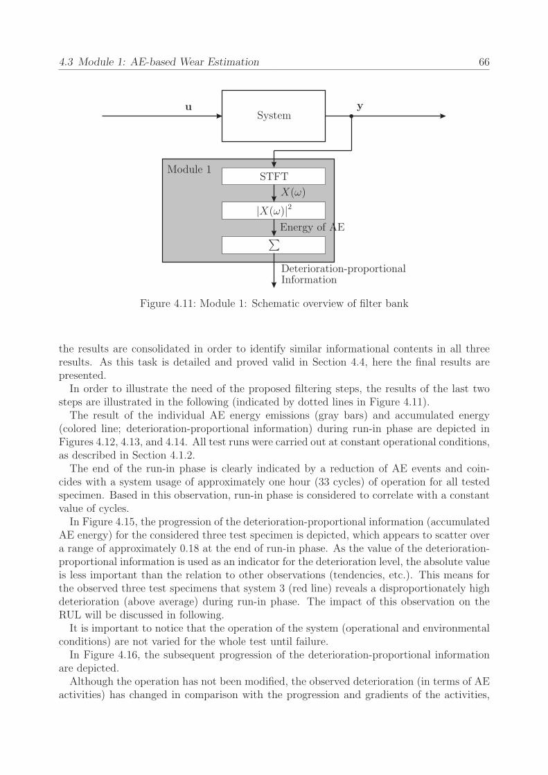
4.3 Module 1: AE-based Wear Estimation 66
u ySystem
Module 1STFT
X(ω)
|X(ω)|2
∑Energy of AE
Deterioration-proportionalInformation
Figure 4.11: Module 1: Schematic overview of filter bank
the results are consolidated in order to identify similar informational contents in all threeresults. As this task is detailed and proved valid in Section 4.4, here the final results arepresented.In order to illustrate the need of the proposed filtering steps, the results of the last two
steps are illustrated in the following (indicated by dotted lines in Figure 4.11).The result of the individual AE energy emissions (gray bars) and accumulated energy
(colored line; deterioration-proportional information) during run-in phase are depicted inFigures 4.12, 4.13, and 4.14. All test runs were carried out at constant operational conditions,as described in Section 4.1.2.The end of the run-in phase is clearly indicated by a reduction of AE events and coin-
cides with a system usage of approximately one hour (33 cycles) of operation for all testedspecimen. Based in this observation, run-in phase is considered to correlate with a constantvalue of cycles.In Figure 4.15, the progression of the deterioration-proportional information (accumulated
AE energy) for the considered three test specimen is depicted, which appears to scatter overa range of approximately 0.18 at the end of run-in phase. As the value of the deterioration-proportional information is used as an indicator for the deterioration level, the absolute valueis less important than the relation to other observations (tendencies, etc.). This means forthe observed three test specimens that system 3 (red line) reveals a disproportionately highdeterioration (above average) during run-in phase. The impact of this observation on theRUL will be discussed in following.It is important to notice that the operation of the system (operational and environmental
conditions) are not varied for the whole test until failure.In Figure 4.16, the subsequent progression of the deterioration-proportional information
are depicted.Although the operation has not been modified, the observed deterioration (in terms of AE
activities) has changed in comparison with the progression and gradients of the activities,

4.3 Module 1: AE-based Wear Estimation 67
Deterioration
-proportion
alinform
ation0.5
0
Energy
ofAEevents
[V2]
10−6
10−4
10−2
1
System usage [number of cycles]0 16 33
Figure 4.12: Acoustic emission energy events (gray bars) and derived progression of deterio-ration-proportional information over system usage for specimen 1 during run-inphase
observed during the first cycles (run-in phase). Therefore, the deterioration behavior of thesystems itself is considered to be changed and denoted by permanent wear phase.Again, system 3 shows a distinct deterioration behavior, as only few but high AE events
(and hence, measured AE energies) determine the curve progression and hence, indicatesevere wear events. The end of permanent wear phase is reached much earlier than forsystems 1 and 2. These systems deteriorate over a long period of cycles before entering thewear-out phase.The last phase of system usage is again ruled by several cycles with noticeable AE events,
ending up with the termination of movement. The exact definition of the transition frompermanent wear phase to wear-out phase is not as unambiguous as from run-in phase topermanent wear phase. Here, the last adjacent AE events are associated to wear-out phaseafter ending up with failure. The individual deterioration progression due to a changeddeterioration behavior during the last phase of system usage are depicted in Figure 4.17.Again, the stochastic aspect of material wear is observed in the scattering instant of failure,
denoted by varying maximum system usages.Once, a sufficiently large number of observations for each particular phase is available, a
quantitative statement can be stated about the correlation between the index and the realdeterioration.Based on the observed behavior, the hypotheses of a correlation between the deterioration
and the observed instant of failure is stated. The analysis result is assumed to be appropriateto describe the incremental deterioration. Hence, the summation of AE energies is a quantity,equivalent to the extent of deterioration.

4.4 Module 2: Average Deterioration Estimation 68
Deterioration
-proportion
alinform
ation0.5
0
Energy
ofAEevents
[V2]
10−6
10−4
10−2
1
System usage [number of cycles]0 16 33
Figure 4.13: Acoustic emission energy events (gray bars) and derived progression of deterio-ration-proportional information over system usage for specimen 2 during run-inphase
In summary, qualitative information are derived from these baseline test. The determi-nation of the current wear phase is important for the estimation of the impact of observedAE events on the state-of-deterioration of the system. Especially the run-in phase is rec-ognized to essentially influence the RUL by (above average) premature deterioration. Thisaspect is important for module 2 to evaluate the probable premature damage due to phase Iand to derive appropriate countermeasures in terms of prolonging the RUL by appropriateoperational conditions.According to Section 3.3, the off-line phase for module 1 is completed as a deterioration-
proportional information is derived and validated in terms of the accumulated AE energy.As observed, the information scatter over system usage as the three systems fail at different,individual instants of system usages with scattering maximum deterioration-proportionalinformation. Hence, the subsequent module 2 gathers the information and derives an appro-priate measure for average, phase-specific deterioration estimation.
4.4 Module 2: Average Deterioration Estimation
The purpose of module 2 is the determination of an average propagation of the deterioration-proportional information by evaluating the past and actual, individual propagation. Basedon the experimentally derived knowledge from module 1, the different, phase-specific deteri-oration progressions (derived under constant operating conditions) are examined. Therefore,each phase is considered and evaluated separately.As introduced in Section 3.4, the unification of the varying deterioration-proportional
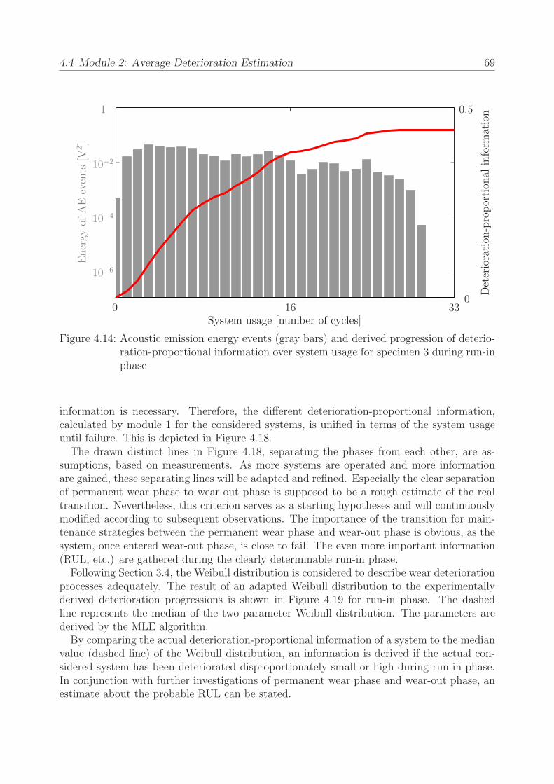
4.4 Module 2: Average Deterioration Estimation 69
Deterioration
-proportion
alinform
ation0.5
0
Energy
ofAEevents
[V2]
10−6
10−4
10−2
1
System usage [number of cycles]0 16 33
Figure 4.14: Acoustic emission energy events (gray bars) and derived progression of deterio-ration-proportional information over system usage for specimen 3 during run-inphase
information is necessary. Therefore, the different deterioration-proportional information,calculated by module 1 for the considered systems, is unified in terms of the system usageuntil failure. This is depicted in Figure 4.18.The drawn distinct lines in Figure 4.18, separating the phases from each other, are as-
sumptions, based on measurements. As more systems are operated and more informationare gained, these separating lines will be adapted and refined. Especially the clear separationof permanent wear phase to wear-out phase is supposed to be a rough estimate of the realtransition. Nevertheless, this criterion serves as a starting hypotheses and will continuouslymodified according to subsequent observations. The importance of the transition for main-tenance strategies between the permanent wear phase and wear-out phase is obvious, as thesystem, once entered wear-out phase, is close to fail. The even more important information(RUL, etc.) are gathered during the clearly determinable run-in phase.Following Section 3.4, the Weibull distribution is considered to describe wear deterioration
processes adequately. The result of an adapted Weibull distribution to the experimentallyderived deterioration progressions is shown in Figure 4.19 for run-in phase. The dashedline represents the median of the two parameter Weibull distribution. The parameters arederived by the MLE algorithm.By comparing the actual deterioration-proportional information of a system to the median
value (dashed line) of the Weibull distribution, an information is derived if the actual con-sidered system has been deteriorated disproportionately small or high during run-in phase.In conjunction with further investigations of permanent wear phase and wear-out phase, anestimate about the probable RUL can be stated.

4.5 Module 3: Wear Prognosis 70
Deterioration
-proportion
alinform
ation 0.5
0
System usage [number of cycles]0 16 33
Figure 4.15: Progression of deterioration-proportional information over system usage for allthree specimen during run-in phase
In comparison to run-in phase, a moderate slope is obtained during this phase which is anindicator for constant wear. Stochastically and severe wear events (in terms of observed AEenergy) is only observed for the this system (red line) after approximately 40% of operationin permanent wear phase.Further studies have to investigate the individual propagations in each phase in more
detail. The phase-specific distribution are modified in terms of their parameters. The mostcritical phase is the run-in phase. Hence, the tests will mainly focus on this phase as itdetermines the remaining life time.
4.5 Module 3: Wear Prognosis
As the parameter space ξ is limited, no extensive tests were carried out to evaluate theinfluence of varying operational parameters on the deterioration (progression) and instantof failure. As this investigation is relevant for further developments, future work shouldconcentrate on selectively changing the operational parameters like material, etc.The deterioration-influencing factors are identified as the type and frequency of lubrica-
tion. As the system operates in a tight industrial network, the arbitrary modification of otheroperational parameters (pressure, velocity of cylinder, etc.) would lead to a decelerated pro-cess and hence to unwanted effects for the preceding and following process steps. Therefore,the focus is set upon the estimation of deterioration and hence, giving deterioration-basedinformation about the probable remaining useful life. This information can subsequently beused to initiate appropriate maintenance strategies and to use the components up to theirmost probable end of life time.

4.6 Summary and Discussion 71
4.6 Summary and Discussion
The failure due to wear of the central functional element of an industrial machine is in-vestigated. According to a detailed material analysis, three main tribological mechanismswhich lead to failure were identified. For investigation purposes, a test rig, which reproducesthe main wear-out effects, was presented. Based on the literature, acoustic emissions wereidentified to be the most promising effect for indicating the deterioration progression.Therefore, a novel measuring chain based on the direct piezoelectric effect was devel-
oped and operated. The main challenges of and solutions for measuring piezoelectricity arediscussed. In particular, the frequency-dependent amplification from source to the digitalcorrespondent was considered within the first filter. Subsequent models used baseline in-formation about typical acoustic emission events to identify relevant signals. This processwas supported by adequate visualization, which indicated the regions and the severeness ofstochastically occurring wear. For the most typical material and lubrication combination,several comparable wear-out tests were performed. A high correlation between the point offailure and the measured damage-equivalent signal was shown.In short, the deterioration under normal operation can be estimated within sufficient
probabilistic limits on the basis of the novel measurement chain and an adequate, FPGAcompatible filter.In the future, different operating parameters can be chosen to support the strategy de-
scribed above. In particular, the database has to be enlarged to cover a larger range ofconditions than the one tested above. To improve the measurement even more, a housedpiezoelectric ceramic reduces the effort of calibration and impedance measurement. Further-more, the effort of gluing several thin layers of identical thickness and material propertieswithout inducing a mechanical strain (deformation) due to mounting can be reduced. Theintegration of the proposed admittance in the electric circuit of the impedance converterimproves the signal-to-noise ratio, and hence signal quality. The admittance of the subse-quent measurement line can be integrated in the FPGA to obtain an even high correlationbetween calculated signal energy and surface displacement. The investigation of individ-ual failure modes (different material changing effects) and correlation with characteristicfrequency ranges, amplitude patterns, etc. can be improved.

4.6 Summary and Discussion 72
Deterioration
-proportion
alinform
ation
0.283
0.288
0.261
0.266
0.443
0.448
0.453
AEEnergy
[V2]
AEEnergy
[V2]
AEEnergy
[V2]
10−6
10−6
10−6
10−4
10−4
10−4
10−2
10−2
10−2
1
1
1
System usage [number of cycles]Begin permanent wear
Begin permanent wear
Begin permanent wear
400
400
400
800
800
800
1200
1200
1200
1600
1600
1600
Figure 4.16: AE power and derived progression of deterioration-proportional informationover system usage for all three specimen, during permanent wear phase
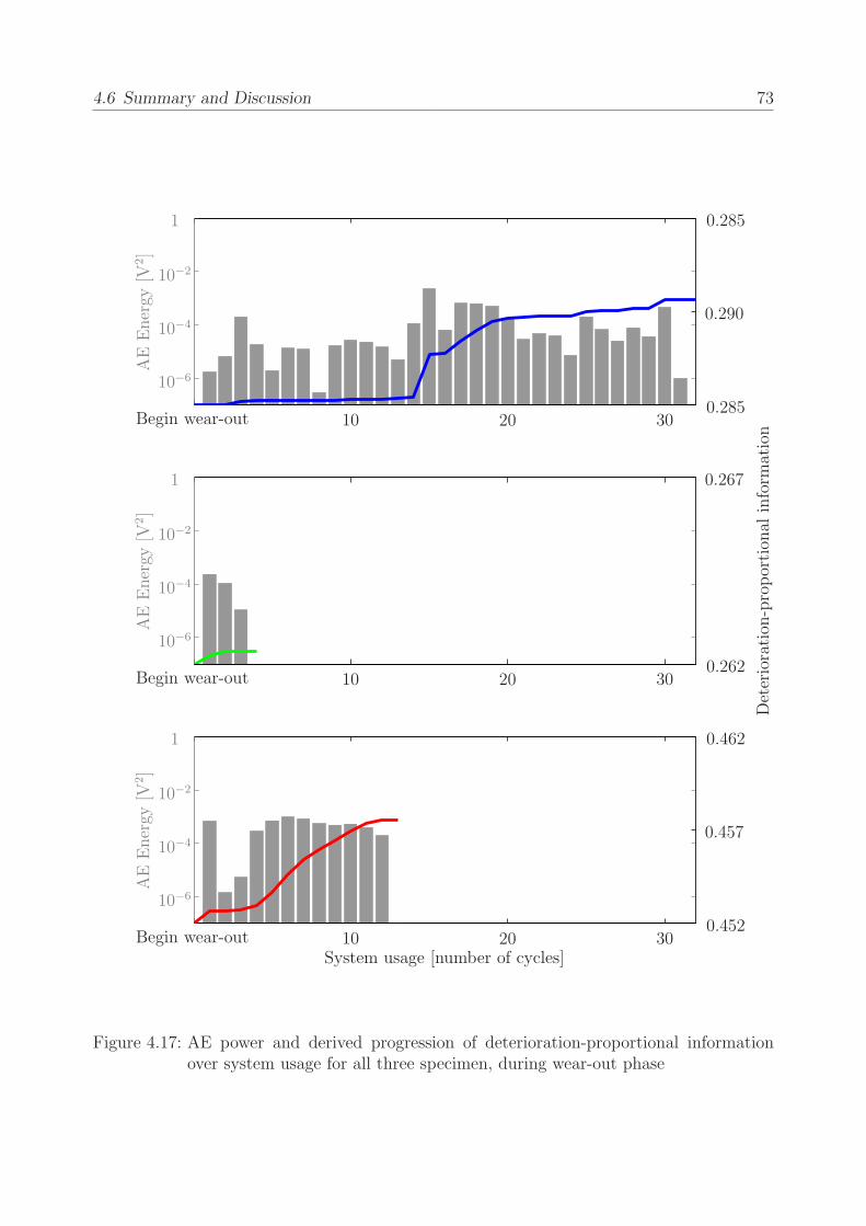
4.6 Summary and Discussion 73
Deterioration
-proportion
alinform
ation
0.285
0.285
0.290
0.262
0.267
0.452
0.457
0.462
AEEnergy
[V2]
AEEnergy
[V2]
AEEnergy
[V2]
10−6
10−6
10−6
10−4
10−4
10−4
10−2
10−2
10−2
1
1
1
System usage [number of cycles]Begin wear-out
Begin wear-out
Begin wear-out
10
10
10
20
20
20
30
30
30
Figure 4.17: AE power and derived progression of deterioration-proportional informationover system usage for all three specimen, during wear-out phase

4.6 Summary and Discussion 74
Deterioration
-proportion
alinform
ation 0.5
0.25
0
Run-in Phase Permanent Wear Phase Wear-out Phase
System usage [%]
0 5 . . . 97 100
Figure 4.18: Normalized progression of deterioration-proportional information over normal-ized system usage with focus on different wear phases
Deterioration
-proportion
alinform
ation 0.5
0.25
0
System usage [%] during run-in phase0 50 100
Figure 4.19: Run-in phase: Progression of deterioration-proportional information
5 Application to Electro-Chemical System
Today, ecological awareness and the attitude towards environmentally harmful technologiesare a central issue. Against the background of off-shore oil production (drilling platforms)and oil transportation and the dire environmental consequences of accidents, finding solutionsfor clean, sustainable energy production is becoming more and more important. Apart fromthe long-term environmental consequences of such disasters (Exxon Valdez, Gulf of Alaska in1989; Deep Water Horizon, Gulf of Mexico in 2010), carbon dioxide production, which mainlyresults from fossil fuel combustion (energy production and road transportation) [RMC+07],contributes to the greenhouse effect. Reducing the main source of these greenhouse gasesmakes a huge contribution to environmental protection.Fossil fuel is mainly used for liquid fuel production, e. g., gasoline, fuel oil, and so on.
Hence, fuel combustion should be reduced to a minimum. Furthermore, as fossil fuel re-sources diminish and an oil crisis is looming, gasoline prices are rising. Increasing pollutionfrom gasoline-powered vehicles is causing major concern about economic and environmentalconsequences. Advanced electric road transportation technologies and sustainable electricityproduction can help to reduce the environmental problems.These aspects inspired the automotive industry to develop novel power train concepts by
integrating a power source and electrical components. Different energy sources (e. g., fuelcells [Jon09], lithium ion accumulators [VNW+05, SCW+09, KBSM09], nickel metal hydrideaccumulators [SCGR05, CSGR06, BSM+07], lead-acid accumulators [SSB+07], etc.) anddifferent topologies for energy flow control were considered [Ozb10]. The advantages anddisadvantages of those concepts are discussed in [Rai09, HH09], for example. In general, allconcepts share the idea of supporting or even substituting the common combustion engineby an electric motor.As a consequence, electricity is the primary source for the novel drive propulsion system.
Besides electricity generation, its storage is obviously becoming increasingly important, asthe energy storage system decisively determines the overall availability, price, and reliabilityof the vehicle. In order to find a compromise between these competing demands and torealize a widely accepted, highly reliable solution, the life time change due to various loadings(operating conditions), individual usage, and at various instants of usage (state-of-X) haveto be evaluated first. Subsequently, smart power management solutions can help to supportthe deterioration-optimal usage of an individual storage system.
5.1 Motivation
In general, batteries are classified into two types: primary (or disposable) batteries areirreversibly discharged. Secondary (or rechargeable) batteries (also called accumulators)can handle both, negative (discharging) and positive (charging) currents. For the intendedapplication of serving as a reusable energy storage systems for novel portable applications,accumulators are considered in the following.
5.1 Motivation 76
Beside the challenge of developing novel low-cost, high-reliable, and safe accumulators thatcan serve as a real alternative to fossil energy sources, the deterioration behavior of actualaccumulators is of interest. As [MFSF09] states, “managing the degradation is particularlychallenging because the associated mechanisms (resistive film growth) [...] are currentlyimpractical as neither a direct access nor a control of the deterioration effects in the cell areavailable.” Since the usage and thus, the degradation of an accumulator, is highly individual,the arising question of how the accumulators deteriorate under varying, non-conform, andunpredictable charge-discharge cycles has to be answered in order to create confidence inthis novel technology. Therefore, the extended SRCE-concept again plays a major role tohelp realizing this ambitious goal of operating the individually aged accumulators such thata maximum usage can be realized.Since the application-specific terminology is used in the sequel, basic definitions of ac-
cumulators are detailed, followed by the description of typical aging processes and effects.Based on the clearly defined task, the SRCE methodology is applied. In Section 5.2 thedeveloped test rig is introduced and the central aspects are illustrated. In contrast to thepreceding chapter, module 1 realizes a model-based fault detection. Again, the focus is setto the estimation of a deterioration measure. In combination with the measurement chain,appropriate tests are designed that reveal relevant deterioration information (physical pa-rameters) and are applicable during field usage. As the validation phase of module 1 reveals arelatively deterministic aging behavior, module 2 plays only a minor role. This might change,if significantly more tests are performed and a scattering quality of the accumulators is ob-served. In Section 5.5, the results of the Design of Experiment (DoE) and Response SurfaceMethod (RSM) reveal a remarkable insight into the deterioration behavior of the consideredaccumulator. Especially with the support of module 1, the deterioration prediction archivesvery good results.
5.1.1 Accumulator Characteristics
Within the domain of accumulator aging phenomenas, the following life time related termsand definitions are used in literature.
Nominal and Actual CapacityThe capacity of an accumulator is a measure for the amount of stored energy that canbe withdrawn from the accumulator and is commonly denoted by C and given in AmpereHours. The capacity, determined by measurement under specific test conditions, is dependedon many operational parameters, amongst others discharge current ID and cell temperatureT [DAS06]. Furthermore, the capacity depends on the state-of-deterioration and is thuscommonly used as an indicator of deterioration. The nominal capacity Cn denotes thecapacity at the beginning of the usage (non-aged state). The actual capacity Ca is determinedat subsequent instants of usage after aging under identical test conditions as used for thedetermination of the nominal capacity.
State of Charge (SoC)The state of charge is a quantity that describes the amount of energy, remaining in the accu-mulator and is commonly given as a percentage of the accumulator’s nominal capacity Cn.As the remaining amount of energy cannot directly be measured, the SoC is approximatedby various methods, e. g., Open Circuit Voltage (OCV) measurement, ampere counting dur-
5.1 Motivation 77
ing charging/discharging, etc. For ampere counting, a higher capacity is determined whendischarging at a low rate than at a high discharge rate. On the other hand, a too low ratewill stimulate self-discharge effects and reduce the efficiency and determined capacity. Theratio between remaining and nominal (or actual) capacity does not represent the state ofcharge accurately.
Depth of Discharge (DoD)The depth of discharge denotes the amount of energy that is withdrawn from the accumu-lator. The DoD describes the complementary characteristic of the SoC and is stated as apercent of the nominal capacity Cn.
State of Health (SoH)The state of health is defined in various ways in order to provide an information about thedegree of deterioration. In general, the state of health is correlated with the actual capacityCa in comparison with the nominal capacity Cn. According to [JW06], the End of Life (EoL,SoH = 0%) time of an accumulator is reached, if the actual capacity Ca is equal than 80%of the nominal capacity Cn.
Calendar LifeThe calender life describes the maximum storage time until the accumulator becomes un-usable (usually considered as a capacity fade of 20%). The storage time is a function ofambient temperature, SoC, etc.
Cycle LifeThe number of complete charge-discharge cycles until the failure criterion is fulfilled (80% ofnominal capacity) is described by the cycle life of an accumulator. Many manufactures statethe cycle life time of an accumulator in dependency of full cycles (number of consecutivecharge-discharge cycles) under optimal operational conditions (C-rates, ambient tempera-ture, rest periods, etc.).
ImpedanceThe behavior of an accumulator as a function of frequency is investigated by the impedancemeasurement. A stimulus (current with varying frequency and alternating direction) is ap-plied to the accumulator and the reaction (voltage) is measured in terms of amplitude andphase shift. As the deterioration process has an (non-linear, state-depended) influence on thefrequency behavior of an accumulator, the Electrochemical Impedance Spectroscopy (EIS)is an appropriate measure to detect faults [Bar05]. In [SG09], “the features extracted fromEIS are used to estimate the internal parameters [...] The values of these parameters [ca-pacitance, resistance, Warburg impedance, electrolyte resistance, etc.] change with variousaging and fault processes.” The impedance curve of an lithium-based accumulator mainlyconsists of an inductive branch at high frequencies, followed by semicircles at medium andlow frequencies [LMWK01]. The intersection of the impedance curve with the imaginaryaxis represents the ohmic resistance of the cell. The physical property is later used as adeterioration measure.
PowerThe power of an accumulator is described by the product of current and voltage. Foraccumulators, the voltage is defined by the cell chemistry (material of anode, cathode, etc);

5.1 Motivation 78
c©SRS, 2011
(a) Normal shape of accumulator
c©SRS, 2011
(b) Accumulator after overcharging
Figure 5.1: Accumulator failure due to overcharging
hence, the ability to provide current makes the difference. Conversely, this means that arising resistance leads to a reduced power. Therefore, peak power tests are common forrough deterioration estimation.
Discharge and Charge Rates (C-rate)It is common practice to characterize the discharge and charge rate as a ratio of the nominalcapacity Cn. The C-rate is given in Ampere. As the field usage of accumulators is usuallyhigher than 1C, the C-rate is an important factor for life time investigations. In [Vez10],the life time of a lithium ion accumulator is reduced by 40% compared to the 1C-rate, if a4C-rate is applied.
TemperatureHigh temperatures facilitate the irreversible reaction between electrode and electrolyte. Re-ferring to the data sheet of the considered accumulators [Gro11], the cells are optimal oper-ated during charging within the range of 0C to 40C, and for discharging within −20C to60C.
Over(dis)chargeThe different, specific chemical potentials of the used materials within an accumulator arethe cause of the cell voltage. A detailed insight into this chemistry aspect of accumulator isgiven in [JW06]. By discharging the accumulator, the chemically stored energy is transformedinto electrical energy and positively charged ions (cations). Within the specified operationalconditions, the electrical energy is provided by the chemically stored energy. By proceedingwith the discharging or charging process, the cell chemistry will sustainable be damaged.The overdischarging scenario assumes a discharging process that is continued beyond the
limits of the specified voltage range. Once all the charge has been drained from the accu-mulator, the electrodes get completely reversed and hydrogen gas builds up, often causingthe accumulator to vent.On the other hand, an overcharge leads to an exothermic reaction within the cell as the
electrically provided energy cannot be stored chemically any more and is thus, transformeddirectly into thermal energy (heating). As the electrolyte starts to vaporize, the pressurewithin the cell continually increases. If the overcharging persists, the gas pressure willincrease enough to burst the cell. In Figure 5.1, the failure due to overcharging is depicted.

5.1 Motivation 79
Cell Specifications Range
End of Charge Voltage UEoC 4.2V ± 0.03VEnd of Discharge Voltage UEoD 2.7VMax. Conti. Charge Current IC,max 20AMax. Conti. Discharge Current ID,max 30AMax. Discharge Rate (30 sec) 50AhNominal Capacity Cn 10AhNominal Voltage Un 3.7VOperation Temperature T −10C . . .+ 55C
Table 5.1: Technical data of KOKAM lithium polymer cell
The aspect of over(dis)charging becomes evident, if a stack of cells is considered. Due tocapacity imbalances, individual cells may fall beneath or rise above the specified operationalconditions and can thus, be destroyed. For this reason, charge equalizing circuits (cellbalancer) takeover the function of avoiding high voltage gradients and hence, preventing anover(dis)charged cell within a stack.
5.1.2 Lithium-Based Accumulators
In the following, the actually most promising storage technology for accumulators basedon lithium is considered. Anyhow, the proposed SRCE-concept is not restricted to thislithium-based accumulators but can again be enlarged to other accumulator technologies.The accumulator investigated in this thesis is a 10Ah Superior Lithium Polymer Battery(SLPB, Model 98106100) by KOKAM in pouch bag. The technical data of the cell are givenin Table 5.1.During charging, the electrical energy is provided to the terminals of the cell. The elec-
trons and lithium ions then move from the cathode through the electrolyte and separatorto the anode. There, the anode (graphite) intercalates the electrons and ions. Beside theintercalation process, the energy is also converted (by side effects) into internal energy lossesand thus, lost in terms of chemical energy. In the opposite case of discharging the accumu-lator, the electrons move through the external load from the anode and are attracted to thecathode. For further explanations about electrodes, electrolytes, additives, and interfaces forvarious cathode and anode materials, typically used for lithium-based accumulators [Oza09]provides a detailed overview.The ideal process of energy conversion in terms of the chemical reaction of a lithium cell
with a lithium cobalt oxide cathode is given in the chemical equations
Anode LiC6
discharge−−−−−−−−−−charge
Li1−xC6 + xLi+ + xe− and
Cathode LiyCoO2 + xLi+ + xe−discharge−−−−−−−−−−charge
Liy+xCoO2 .
In anticipation of the succeeding section, the aging behavior depends “sensitively on indi-vidual cell chemistry and cell design as well as performance data and will vary from battery

5.1 Motivation 80
manufacturer to battery manufacturer”, [WM04]. Thus, the general aging aspects, valid forthe majority of lithium-based accumulators, are discussed in the sequel in order to remainthe global applicability of the subsequently presented results.
5.1.3 Basic Principles of Accumulator Aging
Depending on many factors and particular technologies, accumulators can be rechargedmany times until the recharge ability decreases significantly [BCS+01, Ram03]. Two majoreffects contribute to this aging process: degradation due to storage and due to operation.The primer aspect is not considered here, as the deterioration due to storage contributescomparatively little to the overall deterioration. Additionally, the effect of aging due tostorage can be reduced by keeping the cells close to room temperature, reduced humidityand at average state of charge [RLB+01].For aging due to operation, two main basic aging effects are encountered when dealing
with lithium-based accumulator: power and/or capacity fade [Pic07]. If only the formerdegradation effect is present, the accumulator is capable of supplying all the stored energy,but reveals the lack of capability of providing a high current. For the latter degradationeffect, a high current can still be withdrawn from the accumulator after aging but cannotdeliver all the stored amount of energy.The reasons for this aging effects are manifold but all base on different (non-linear, stochas-
tic) electro-chemical processes, taking place in parallel. “In general, the situation reportedin the literature is difficult to analyze as each lithium-ion cell system has its own chemistryand many aging effects are influenced by the nature of the cell components (e. g., activematerial and electrode design, electrolyte composition, impurities, etc.)”, [VNW+05].In Figure 5.2, a graphical overview about the main deteriorating effects is given, depicting
the major aging effects as mentioned in [MFSF09, BMFF11, RHG+04, VNW+05].At the anode side, three different deterioration effects are depicted. All effects are a result
of the chemical reaction taking place at the interface between the electrode (here: graphite)and electrolyte, particularly during charging. At the beginning of cycling, a protective layerbuilds up that covers the electrode (formation phase). The layer is a decomposition productof the reductive reaction of the electrolyte (gray circles), taking place during charging. Ifthe layer realizes a protective function, the layer is denoted as the Solid Electrolyte Interface(SEI) Film (light yellow). During this phase, a slightly increasing capacity is measured.The film is permeable for lithium ions (red circles; intercalation and deintercalation), butnearly impermeable for electrolyte components. Hence, this layer realizes a desired functionin order to reduce further reduction of the anode. On the other side, the amount of mobilelithium is reduced as chemically bonded to the SEI Film and hence, the performance of theaccumulator is reduced. The film has a time and spatially varying thickness. Accordingto [VNW+05, ACL+01, SLWW02, LMWK01, ZHD+00, ZW08], the film growth contributesto a capacity and power fade and an increased impedance. If the protective function cannotbe realized due to inhomogeneous current and potential distributions within the cell, lithiumions and electrolyte intercalate into the graphite and cause an irreversible damage to thestructure (graphite exfoliation, cracking). Already intercalated lithium ions may be trappedand thus, lost. Finally, the lithium can corrode the interface of the electrolyte and theelectrode, form a metal plating, and permanent capacity loss (wear-out phase). The metalliclithium forms dendrites that grow until penetrating the separator and contacting the cathode;

5.1 Motivation 81
+-
Oxidation of Conductive
Particles and Corrosion of
Current Collector
Micro-Cracking
Graphite Cobalt Oxide
SEI Film
Lithium Plating,
Graphite Exfoliation, Cracking
Dissolution
Separator
Lithium-Ion
CurrentCollector
CurrentCollectorwith Solvent
Corrosion
Figure 5.2: Overview on main aging mechanism within a lithium-based accumulator
a short-circuit of the cell is realized and an explosion is likely to occur.On the right side of Figure 5.2, the deteriorating effects of the cathode are depicted.
As the cathode material significantly determines the deterioration behavior, only globallyvalid statements about general effects are discussed in the sequel. In analogy to the anode,the cathode material is stressed by the intercalation and deintercalation of lithium duringcharging and discharging. As lithium ions are inserted into the active material (light blue)during discharging, the lithium may induce mechanical stress and strains to the oxide par-ticles [VNW+05]. A direct consequence is a structural change and thus, the (micro) crackformation. Encouraged by inhomogeneous chemical reactions, persisting micro cracks and adistorted crystal lattice, the bulk material can dissolute into the electrolyte. As this processescan also take place at the conductive interface between the active material and the currentcollector, the contact loss also contributes to a reduced capacity and power performance.In summary, the majority of research work accounts the changes at the interface between
the anode (graphite electrode) and the electrolyte for being mainly responsible for the ag-ing [VNW+05, BBB+05]. As manifold drivers of deterioration occur in parallel “and cannotbe discussed independently from each other” [WM04], the overall deterioration is evaluated

5.2 Measurement Chain 82
from (directly measurable) physical properties. Here, the internal resistance at specific fre-quencies is measured and is considered as the major measurable indicator of a decreasingaccumulator performance. This idea is supported by various research work in literature,e. g., in [RBM+10] where the health-governing cell degradation indicator is identified as the“increase of the internal resistance of the battery cells over the whole life time of the bat-tery.” The resistance is identified “with the special identification signals of terminal voltageand current.” Subsequently, the variation of the resistance is used to state a degradationindex.
5.2 Measurement Chain
The purpose of the test bench is to conduct reliable aging experiments on lithium accumu-lators. The test benches will be operated automatic and unattended since the tests will takelarge amounts of time. This in turn requires the test benches to be safe.After a short introduction into the test rig and its specifications, typical measurements are
discussed. The implicit measurement of deterioration (change of internal resistance, actualcapacity, etc.) is introduced and illustrated with experimental examples. By repetitivelycharging and discharging the accumulator with specifically designed aging cycles, small butpermanent damages are stimulated that cause the accumulator to never regain its originalperformance.
5.2.1 Test Rig
A novel test rig is developed such that arbitrary charge and discharge profiles can be appliedto the accumulator (KOKAM cell, technical data see Table 5.1) and special tests for param-eter estimations (see module 1) can be performed. In Figure 5.3, a schematic representationof the developed test rig for accumulator aging is depicted.The central component is the accumulator. Since the genuine aging of an accumulator
without disturbing effects due to additional balancing are investigated, a single cell is used.The surface temperature of the cell is measured by a NiCrNi temperature element (temper-ature range from −30C . . .+100C) and linearly transformed into a voltage (0V . . .+10V).The cell voltage is measured at the terminal clamps of the cell. A buffer amplifier is usedto transform the input voltage (maximum range: −5V . . . + 5V) into an adequate outputvoltage (10V . . .+ 10V).In order to automate the test procedure, an electric switching between charging and dis-
charging is realized by an electronic power switch (semiconductor, solid-state relays). Independency on the operation, the electrical circuit is closed with the power source (forcharging the accumulator), the electronic load (for discharging purpose) or left open (foridle mode). In the case of an power shortage of the processes control unit and hence, lostof control, the switch automatically opens and disconnects all devices from each other (failsafe).Charging is accomplished using a DC power supply. The power source is capable for
currents up to 20A and 65V. The nominal values and actual values for current and voltageare externally controllable and measurable.An electronic load is used to withdraw current from the accumulator. The device can
realize a discharge current between 10mA to 50A within a voltage range of 2.5V to 80V. In

5.2 Measurement Chain 83
ADC
ADC
ADC
ADC
DAC
DAC
DAC
++
+
--
-
Volt.-
Sensor
Temp.-
Sensor
Switch
Load Source
ICId
Accumulator
Figure 5.3: Test rig for accumulator testing
analogy to the power source, the relevant process signals are controllable and measurablefrom an external source. Beside the specifications for current and voltage, the reaction speedof the load is important in order to realize the required measurements (step response). Thisparticular device is able to realize a step demand within less than 100µs.The process signals are connected either by analog-digital converts (ADC) or digital-
analog converters (DAC) to a real-time process control system (dSPACE, not depicted)in order to control remotely the load and power supply. Arbitrary current profiles andcharge controllers can be realized in Matlab
R©/Simulink R© and are then applied to theaccumulator through the power supply and electronic load. The data acquisition and controlis accomplished using Matlab
R©/Simulink R© software such that the measured input signalsare processed to realize particular test sequences, e. g., discharge and charge trajectories andsupervision purposes, e. g., cell temperature. Furthermore, all relevant process signals arerecorded in order to analyze the data for deterioration content, extract relevant parametersfor subsequent models, etc. Additionally, life time models can be implemented to on-linesupervise the actual (incremental) deterioration due to applied loading.
5.2.2 Aging Cycles
The purpose of the aging cycle, consisting of charging and discharging, is to specificallystimulate the aging effects and causing an incremental deterioration at each cycle. In antici-pation of modules 1 and 3, the framework of the used aging cycles is briefly introduced here.The justification for the particularly chosen parameters (for charging, discharging, etc.) isgiven in Chapter 5.5.

5.2 Measurement Chain 84
IC,max
ID,max
0
Current
UEoC
UEoD
Voltage
t1 t2 t3 t4Time
CC-charging CV-charging Discharging
Figure 5.4: Standard aging cycle
The standard scheme of a current profile with resulting voltage curve is given in Figure 5.4.This standard cycle is varied such that different purposes are fulfilled.First, the standard charging procedure for lithium-based accumulators is described by
this standard representation. A constant current is applied until the accumulator voltageU reaches UEoC = 4.2V. Then, the voltage is kept constant until the current drops toIC ≤ 50mA. This procedure is denoted as the CC-CV (constant current-constant voltage)charging procedure. Referring to [Gro11], the optimal key data for the charging profile aregiven as 10A and UEoC = 4.15V.Secondly, the parameters, defining the key data of charging (IC, UEoC, and UEoD) can be
varied in order to optimize the usability and/or availability of the accumulator by enhancingthe recharging time, etc.The discharging profile in field usage is individual and hardly predictable. Therefore, test
parameters with maximum performance are chosen in order to test for maximum loadingcapacity. The discharging procedure is defined such that the accumulator is discharged at aconstant C-rate. As the terminal voltage U reaches the end of discharge voltage UEoD = 2.7V,the discharging is stopped. Due to the limited rate of diffusion of ions through the electrolyte,the efficiency of an accumulator varies at different discharge rates. Again, [Gro11] proposes

5.2 Measurement Chain 85
30
30
15
15
0
0
-15
-15
-30
-30
Current[A
]Current[A
]
4.5
4.5
4
4
3.5
3.5
3
3
2.5
2.5
Voltage
[V]
Voltage
[V]
0
0
0.25
0.25
0.5
0.5
0.75
0.75
1
1
1.25
1.25Time [h]
CC-charging
CC-charging CV-charging
CV-charging Discharging
Discharging Idle
Figure 5.5: Charging and discharging behavior of an accumulator;Upper plot in non-aged state, lower plot in aged state
optimal key data for the discharging that remain below the maximum ratings. The dischargeis performed with ID = 10A and UEoD = 3V.As these parameters determine the operation, the variation of the charging and discharging
parameters are considered to considerably influence the life time.In Figure 5.5, the result of the application of the aging profile is depicted. The CC-CV
charging is exemplarily shown at a C-rate of 1.5C; the subsequent discharging is performedat 3C. In the upper plot, the behavior of the accumulator at the non-aged state is illustratedwhere the lower plot depicts the result at the aged state (identical cell). The shape andduration of each charging and discharging phase varies in dependency on the SoH. By varyingthe particular operational parameters of the aging profile, the accumulator will individuallydeteriorate and provide an insight into the deterioration progression. The deterioration-depended behavior during charging and discharging is quantified in the sequel by appropriatetest procedures.

5.2 Measurement Chain 86
81.4_______100% SoH81.4% SoH
State of Charge [%]
Open
CircuitVoltage
[V]
3.0
3.5
4.0
0 10 20 30 40 50 60 70 80 90 100
Figure 5.6: Measurement of SoC-OCV curve; red line denoting non-aged cell, the gray lineaged cell
5.2.3 Measurement of Deterioration
In order to assess the individual aging of the accumulator due to the above introduced agingprofile, deterioration measurements (in terms of determination of relevant electrical parame-ters, e. g., internal resistance, actual capacity, etc.) are performed for each cell before startingthe aging cycles. For the validation of the later introduced model, these test are conductedperiodically. By comparing the results (measurement and calculation results) along withthe accumulators life time, the aging gets evident. By performing these measurements afterknown operational trajectories (in terms of operational parameters, number of successiveaging cycles) the incremental deterioration due to the applied loading can be determined atvarious (discrete) initial states of deterioration.The aim is to provide deterioration-relevant information to the subsequent module in
order to investigate the impact of the aging cycles on the accumulator performances. Alltested accumulators are selected from one batch. After the initial measurement, the agingcycles are performed several times. Then, all of the below described measurement cycles areperformed, before starting again with the aging cycles.
SoC-OCV MeasurementAs Figure 5.4 indicates, the terminal voltage rises with increasing charge. This suggests thatthe voltage can be correlated to the State of Charge. Since the State of Charge is in turnconnected to the State of Health, a typical SoH indicator is derived from the connectionbetween the Open Circuit Voltage (OCV) and the State of Charge (SoC). To measure theOCV, a measurement cycle is developed and applied as followed:
1. Discharge 5% of charge with ID = 30A for 60s.
2. Idle mode (20 minutes)
The accumulator is assumed to be fully charged and rested for a sufficient period of timein order to cool down and let chemical processes taking place. The scheme is repeated untilthe accumulator is fully depleted (UEoD reached; theoretically 20 times). For the proposedtest scheme, the SoC-OCV curve is measured every 5% of SoC. The corresponding voltage ismeasured after the idle mode. A typical result, consisting of 20 measurements, is depicted in

5.2 Measurement Chain 87
Figure 5.6. The equally spaced measurement points are connected by an interpolating line;the red curve denotes an non-aged accumulator whereas the blue curve shows the result foran aged accumulator (SoH approx. 80%).The slope of the curve is commonly denoted by the factor k. It is obvious that the
correlation between OCV and SoC is possible but not very sensitive to the deterioration asboth curves only slightly differ (in terms of k) from each other.
Capacity MeasurementAs the overall degradation is of interest, the ampere counting method is an indicator toestimate the actual capacity Ca. Although the measurement is time consuming and “leadslittle possibility for on-the-fly on-board vehicle assessment, [...] it is the best way to assessbattery life” [Pic07]. To avoid energy loss due to thermal dissipation (energy dissipatingeffects like heating due to chemical reactions [DAS06]), the discharging and charging isconducted at very slow rates (e. g., ID = C/20-rate). Additionally, the accumulator has torest in between the charging and discharging period; in literature, time periods up to 24 hoursare described as sufficient. Following these recommendation, the complete measurementcycle lasts for approximately 50 hours. By comparing the obtained value with previousmeasurement result (e. g., with nominal capacity Cn), the fade of capacity becomes obvious.In this thesis, the main interest is dedicated to the gradient (change) of deterioration due
to operation. The counted ampere hours are neither completely stored into chemical energyduring charging, nor is the drained energy completely converted to electrical energy but alsocomprises thermal energy. Thus, an average capacity is determined by ampere counting ofboth, charging and discharging currents.
Measurement of Electrical ParametersIn contrast to the application example, discussed in Chapter 4, here, physical properties,indicating the degree of deterioration, are implicit measurable by specially designed testprocedures under standardized conditions. The methods for acquiring the relevant electricalparameters are based in the research work of [WZX09].The basic idea constitutes that the impedance changes characteristically with a decreasing
SoH. Thus, the internal resistance of the cell is measured in order to investigate the result fordeterioration content. In conjunction with the equivalent circuit (model), depicted in Fig-ure 5.8, three deterioration-depended parameters have to be evaluated: the ohmic resistanceRo, the polarization capacity Cp, and the polarization resistance Rp.For the determination of the primer resistance, a peak current measurement is applied in
order to measure the voltage response of the accumulator to a discharge current step. InFigure 5.5 the effect of a peak current measurement is shown. The voltage drop of the agedaccumulator (lower plot) differs significantly from the nominal behavior (upper plot). InFigure 5.7, the voltage drop is depicted (characteristic points U0 and U1).The result is the ohmic resistance Ro, measured as the voltage drop at the current step
Ro =U1 − U0
ID. (5.1)
After the voltage drop due to the ohmic resistance, the capacitive properties become dom-inant. After stopping the discharging, the voltage raises again rapidly to U3 and propagatesasymptotically to the final (open circuit) voltage U4.

5.3 Module 1: SoH Estimation 88
Time [s]
Voltage
[V]
4.2
4.1
4.0
3.9 0 0.2 0.4 0.6 0.8 1.0
U0
U1
U2
U3
U4
Figure 5.7: Voltage drop as the reaction on a discharging current step
According to [CV05], the polarization resistance is determined by this measurement as
Rp =U2 − U1
ID, (5.2)
and the capacity is
Cp =τ
Rp
. (5.3)
According to [VPB07], the polarization time constant τ is derived by
τ = −∆t ln
(1− U4 − U3
U0 − U3
), (5.4)
with ∆t indicating the discharging time (here: 0.5s).
Measurement of TemperatureThe temperature gradient also reveals a characteristic behavior along with an increasingaging as the temperature rises more rapidly when the accumulator is aged. This symptom isreducible to the common entity, the varied internal resistance. Hence, the measurement ofthe internal resistance (as the cause of the temperature increase, varying voltage drop, etc.)is assumed to be a major indicator of deterioration.
5.3 Module 1: SoH Estimation
Referring back to the intended application (electrical storage and source for automotive ap-plication), the charge and discharge profiles are the major life time determining factors. Incontrast to manufacturer information, an accumulator in field usage will fail earlier due toindividual, non-optimal charge and discharge trajectories than specified. Hence, a model,approximating the actual state of health (SoH), needs to consider (amongst other factors)the past loading and their specific (incremental) effects on the life time. The task of mod-ule 1 is thus to provide a sufficiently precise and accurate filter that is based on availablemeasurements of deterioration-effected physical parameters.

5.3 Module 1: SoH Estimation 89
Rp
Cp
Up
+
−
U
Ro
Uo
UOCV(SoC)
I
I1
I2
Figure 5.8: Equivalent circuit diagram with lumped parameters of an accumulator [WZX09]
Several models for estimating the deterioration behavior of an accumulator are discussedin literature.In [BCL+05, SW08], an adapted model is proposed to accumulate an incremental damage.
By introducing experimentally determined factors, the deterioration behavior is approxi-mated. The main drawback of the proposed model is that it static and thus, not capable ofconsidering aging effects.In [SG08, SG09, SGPC09], a Bayesian approach is discussed. The Bayesian models are
used in order to state the probability “as the degree of belief that a proposition is true.”As the Bayesian PDF adapts to the change in data, this technique is also denoted as self-correcting. This ability to adapt to novel situation (e. g., changed data base) is used toconstruct an adaptive battery health monitoring approach. The deterioration predictionis supported by the particle filter approach that estimates “the evolution in time of thesystem under analysis.” The particle filter “is a technique for implementing a recursiveBayesian filter using Monte Carlo (MC) simulations [...].” In summary, the method considersa non-exact, non-linear, and non-stationary model with non-Gaussian noise. The shownresults are promising, but the method is time-consuming and requires intensive experimentalinvestigations of accumulator behavior.The applied model, detailed in the following, is a simplified Randles-circuit [Ran47],
introduced by [Kim10], as it reveals the main information for deterioration estimation. Themain advantage of this model is that physical properties (e. g., ohmic restistance) are mea-sured only once (at beginning of life time) and subsequently intentionally kept constant inorder to deduct the erroneous system behavior due to the deviation in calculated and mea-sured output quantity performance. Thus, the model focuses on the detection of a variedimpedance due to deterioration. Although, the (physical, chemical) sources of an increasingimpedance are manifold, only the effect is considered in the sequel. Therefore, a model ofthe accumulator is chosen that considers the relevant electrical effects at a macroscopic levelin order to reduce the modeling and numerical efforts.The main components of the model, depicted in Figure 5.8, are the non-linear voltage
source UOCV(SoC), an ohmic resistance Ro, and a RC model, constituted by the polarization
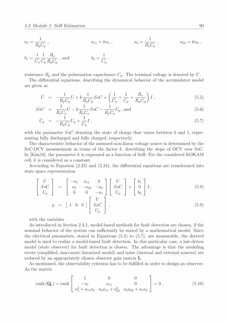
5.3 Module 1: SoH Estimation 90
a1 =1
RpCp
, a11 = ka1 , a2 =1
RoCn
, a22 = ka2 ,
b1 =1
Cn
1
Cp
Ro
RpCp
, and b2 =1
Cp
.
resistance Rp and the polarization capacitance Cp. The terminal voltage is denoted by U .The differential equations, describing the dynamical behavior of the accumulator model
are given as
U = − 1
RpCp
U + k1
RpCp
SoC +
(1
Cn
+1
Cp
+Ro
RpCp
)I , (5.5)
˙SoC =1
RoCn
U − k1
RoCn
SoC − 1
RoCn
Up , and (5.6)
Up = − 1
RpCp
Up +1
Cp
I , (5.7)
with the parameter SoC denoting the state of charge that varies between 0 and 1, repre-senting fully discharged and fully charged, respectively.The characteristic behavior of the assumed non-linear voltage source is determined by the
SoC-OCV measurement in terms of the factor k, describing the slope of OCV over SoC.In [Kim10], the parameter k is expressed as a function of SoH. For the considered KOKAMcell, k is considered as a constant.According to Equation (2.23) and (2.24), the differential equations are transformed into
state space representation
˙
USoCUp
=
−a1 a11 0a2 −a22 −a20 0 −a1
USoCUp
+
b10b2
I , (5.8)
y =[1 0 0
]
USoCUp
, (5.9)
with the variablesAs introduced in Section 2.4.1, model-based methods for fault detection are chosen, if the
nominal behavior of the system can sufficiently be stated by a mathematical model. Sincethe electrical parameters, stated in Equations (5.5) to (5.7), are measurable, the derivedmodel is used to realize a model-based fault detection. In this particular case, a law-drivenmodel (state observer) for fault detection is chosen. The advantage is that the modelingerrors (simplified, inaccurate linearized model) and noise (internal and external sources) arereduced by an appropriately chosen observer gain matrix L.As mentioned, the observability criterion has to be fulfilled in order to design an observer.
As the matrix
rank (Qo) = rank
1 0 0−a1 a11 0
a21 + a11a2 a2a11 + a222 a2a22 + a1a2
= 3 . (5.10)
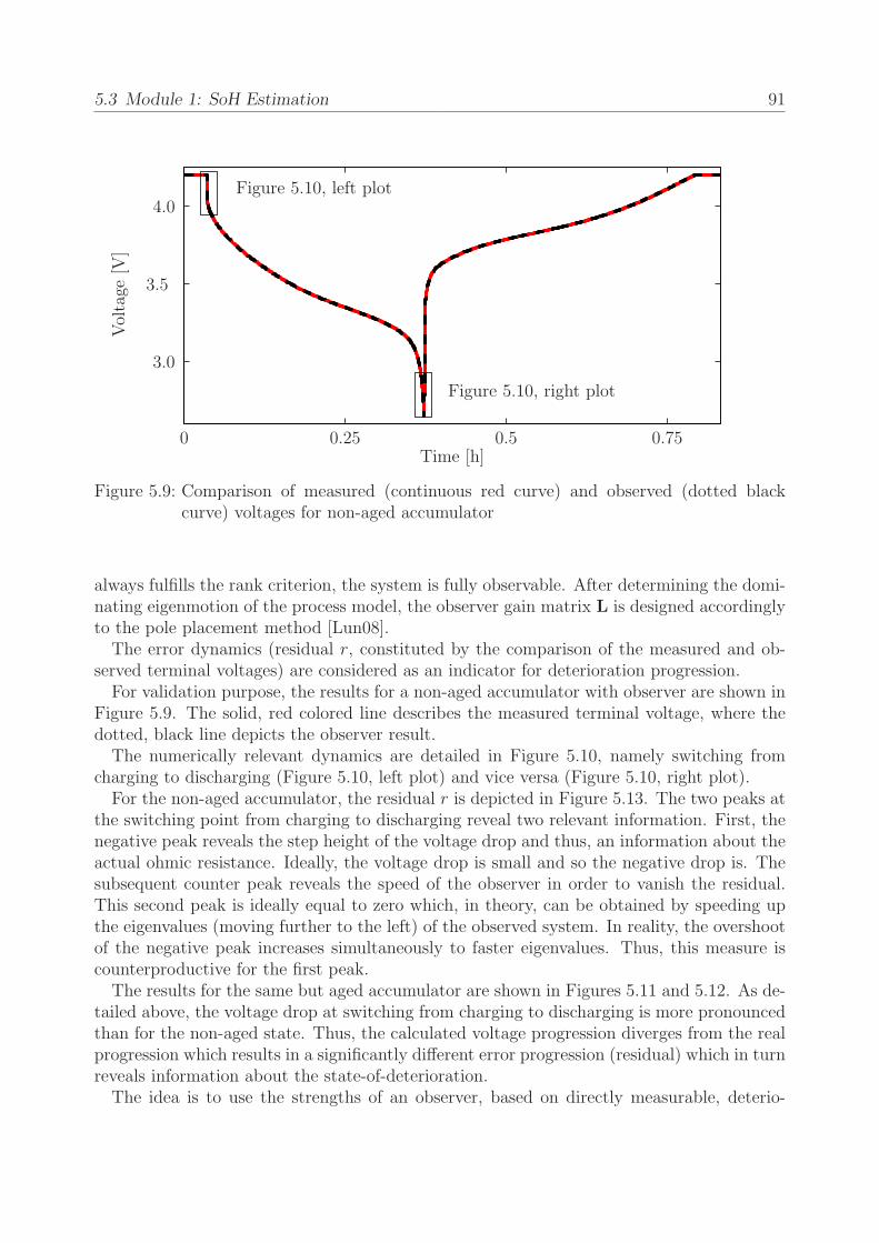
5.3 Module 1: SoH Estimation 91
Figure 5.10, left plot
Figure 5.10, right plot
Voltage
[V]
Time [h]
4.0
3.5
3.0
0 0.25 0.5 0.75
Figure 5.9: Comparison of measured (continuous red curve) and observed (dotted blackcurve) voltages for non-aged accumulator
always fulfills the rank criterion, the system is fully observable. After determining the domi-nating eigenmotion of the process model, the observer gain matrix L is designed accordinglyto the pole placement method [Lun08].The error dynamics (residual r, constituted by the comparison of the measured and ob-
served terminal voltages) are considered as an indicator for deterioration progression.For validation purpose, the results for a non-aged accumulator with observer are shown in
Figure 5.9. The solid, red colored line describes the measured terminal voltage, where thedotted, black line depicts the observer result.The numerically relevant dynamics are detailed in Figure 5.10, namely switching from
charging to discharging (Figure 5.10, left plot) and vice versa (Figure 5.10, right plot).For the non-aged accumulator, the residual r is depicted in Figure 5.13. The two peaks at
the switching point from charging to discharging reveal two relevant information. First, thenegative peak reveals the step height of the voltage drop and thus, an information about theactual ohmic resistance. Ideally, the voltage drop is small and so the negative drop is. Thesubsequent counter peak reveals the speed of the observer in order to vanish the residual.This second peak is ideally equal to zero which, in theory, can be obtained by speeding upthe eigenvalues (moving further to the left) of the observed system. In reality, the overshootof the negative peak increases simultaneously to faster eigenvalues. Thus, this measure iscounterproductive for the first peak.The results for the same but aged accumulator are shown in Figures 5.11 and 5.12. As de-
tailed above, the voltage drop at switching from charging to discharging is more pronouncedthan for the non-aged state. Thus, the calculated voltage progression diverges from the realprogression which results in a significantly different error progression (residual) which in turnreveals information about the state-of-deterioration.The idea is to use the strengths of an observer, based on directly measurable, deterio-

5.3 Module 1: SoH Estimation 92
Charging → Discharging Discharging → Charging
Voltage
[V]
Time [s]Time [s]
4.0
4.1
4.2
2.70
2.72
130.57 131.16 1342.05 1342.51
Figure 5.10: Details of relevant dynamics for non-aged accumulator
ration-effected physical properties, in combination with a subsequent signal-based decisionmaking. This method is practicable as it can be applied during operation of the accumulatorwithout connecting any additional measurement devices.The second couple of peaks at the switching from discharging to charging reveals the same
information but the other way round: first, a positive peak is obtained, as the real voltagesuddenly raises. This is subsequently compensated by the observer, again in dependencyon the designed eigenmotions. The same holds true for the above mentioned challengeof overshoot. Therefore, a balance between speed and damping is found by placing theeigenvalues two times faster than the dominating eigenvalues of A.In Figure 5.14, the correlation between two, independently from each other derived infor-
mation about the state-of-deterioration are depicted. The blue curve denotes the progressionof the actual capacity Ca (measured by ampere counting method after each 30 consecutive ag-ing cycles), approximated by linear interpolation between the discrete values. After slightlyincreasing at the first intervals (formation phase), a constant capacity loss (negative, con-stant gradient) is observed. At approximately 250 cycles, the wear-out phase is entered andthe degradation increases disproportionately. The actual capacity drops below the criticalcapacity of 8Ah (= 0% SoH).Independent of the capacity measurement, similar deterioration information are obtained
by the model-based fault detection. The depicted residual progression is obtained by string-ing together the first peak due to varying ohmic resistance (Figure 5.13) of each aging cycle.The envelope of this peaks is depicted as the bold black curve and constantly increases untilthe same characteristic point of 250 cycles. Short before that point, the curve characteristicchanges from a linear to a exponential shape. As the end of life is reached (SoH = 0%), theabsolue value of the residual is approxemately 0.32V.In the simplest case, the actual state-of-deterioration is obtained by performing the pro-
posed peak current measurements at fully charged condition and observing the residual. As

5.4 Module 2: Confidence Check 93
Figure 5.12, left plot
Figure 5.12, right plot
Voltage
[V]
Time [h]
4.0
3.5
3.0
0 0.25 0.5 0.75
Figure 5.11: Comparison of measured (continuous red curve) and observed (dotted blackcurve) voltages for aged accumulator
demonstrated, the residual behaves inversely proportional to the SoH (defined as the rationbetween actual and nominal capacity) and is thus, applicable for deterioration investigations.In summary, the proposed mathematical model, describing continuously the deterioration-
depended behavior of the considered accumulator, in combination with an appropriatelydesigned model-based fault detection method (observer) is capable of describing the voltagecurve due to a charging and discharging current. Furthermore, the obtained residual revealsinformation about the chosen eigenvalues of the observer (dynamic, overshoot) as well as thestate-of-deterioration (voltage drop due to changed, ohmic resistance) of the accumulator.The relevant physical parameters can easily be measured by standard sensors and speciallydesigned test cycles in order to validate the method. Since only the nominal capacity Cn
is relevant for the observer-based on-line fault detection, the time-consuming measurementof the actual capacity Ca, as described in Section 5.2.3, is obsolete. Nevertheless, thisinformation will additionally be provided in the subsequent modules in order to validate thisassumption.
5.4 Module 2: Confidence Check
As stated in Section 3.4, module 2 plays a minor role for this particular system as the deteri-oration (capacity fade) is measurable. Hence, module 2 is less important in this context andonly serves as a plausibility check whether or not the measured and observed deteriorationprogressions coincide.The distribution of the initially measured ohmic resistance (and hence feature) is depicted
in Figure 5.15.Although the tested cells originate from the same batch, differences in the physical param-
eters are measured. The test specimen are chosen such that the scattering is relatively small.
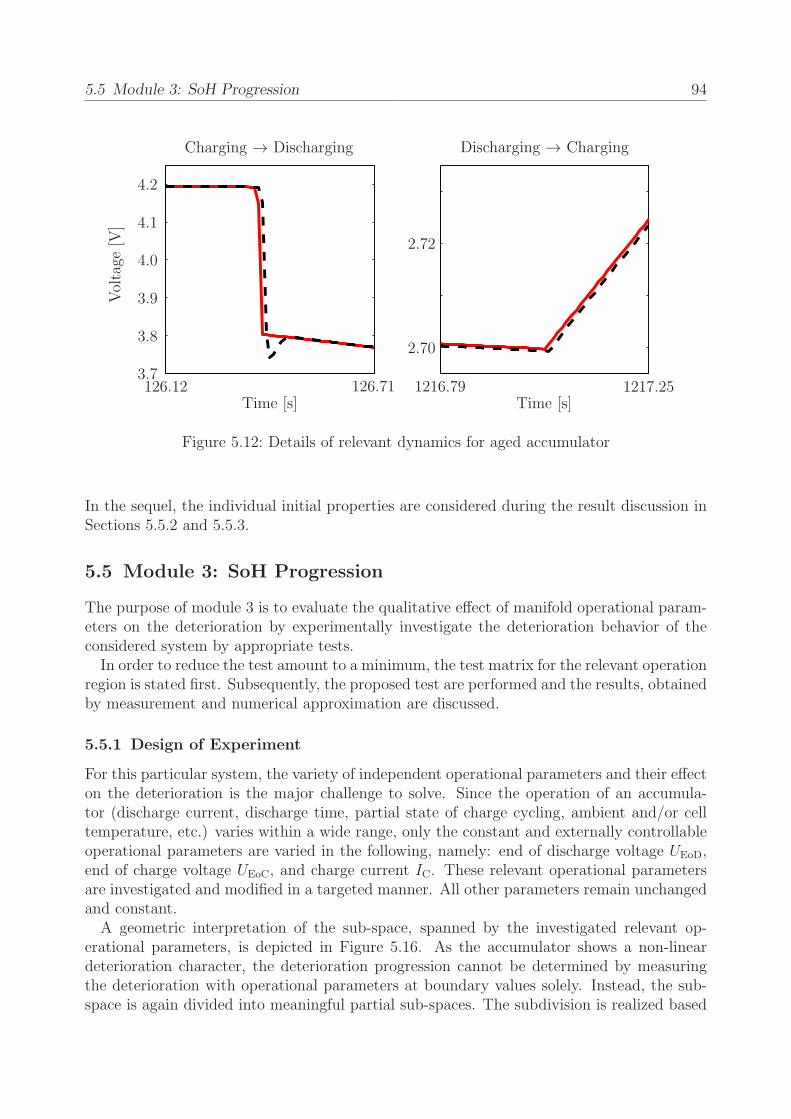
5.5 Module 3: SoH Progression 94
Charging → Discharging Discharging → Charging
Voltage
[V]
Time [s]Time [s]
3.7
3.8
3.9
4.0
4.1
4.2
2.70
2.72
126.12 126.71 1216.79 1217.25
Figure 5.12: Details of relevant dynamics for aged accumulator
In the sequel, the individual initial properties are considered during the result discussion inSections 5.5.2 and 5.5.3.
5.5 Module 3: SoH Progression
The purpose of module 3 is to evaluate the qualitative effect of manifold operational param-eters on the deterioration by experimentally investigate the deterioration behavior of theconsidered system by appropriate tests.In order to reduce the test amount to a minimum, the test matrix for the relevant operation
region is stated first. Subsequently, the proposed test are performed and the results, obtainedby measurement and numerical approximation are discussed.
5.5.1 Design of Experiment
For this particular system, the variety of independent operational parameters and their effecton the deterioration is the major challenge to solve. Since the operation of an accumula-tor (discharge current, discharge time, partial state of charge cycling, ambient and/or celltemperature, etc.) varies within a wide range, only the constant and externally controllableoperational parameters are varied in the following, namely: end of discharge voltage UEoD,end of charge voltage UEoC, and charge current IC. These relevant operational parametersare investigated and modified in a targeted manner. All other parameters remain unchangedand constant.A geometric interpretation of the sub-space, spanned by the investigated relevant op-
erational parameters, is depicted in Figure 5.16. As the accumulator shows a non-lineardeterioration character, the deterioration progression cannot be determined by measuringthe deterioration with operational parameters at boundary values solely. Instead, the sub-space is again divided into meaningful partial sub-spaces. The subdivision is realized based

5.5 Module 3: SoH Progression 95Residual
[V]
Time [h]
Peak due to observer dynamic
Peak due to ohmic resistance
0.15
0
0-0.15
0.25 0.5 0.75
Figure 5.13: Feature progression (residual r)
End of Discharge Voltage [V] UEoD 2.65 2.70End of Charge Voltage [V] UEoC 4.20 4.25Charge Current [A] IC 15 20
Normalized Factors xi −1 +1
Table 5.2: Operational parameters and assignment to normalized factors
on observed field-relevant usage profiles (accumulation of parameter constellations). Theseconstellations are depicted in Figure 5.16 as red points within the cuboid.As no field data are available, it is assumed that the accumulator will be charged as fast
as possible (high charging current IC) to the maximum possible end of charge voltage UEoC
and discharged as far as possible to the minimum possible end of discharge voltage UEoD.Thus, the region of densest accumulation of relevant operational parameter constellations islimited and given in Table 5.2.This relevant partial sub-space is depicted in detail in Figure 5.17. Within this sub-sub-
space, it is assumed that the deterioration behavior can be approximated by deteriorationinformation from measurement results at boundary values xi = −1 and xi = +1.The designed test sequence consists of the measurement of relevant deterioration infor-
mation and the subsequent aging of the cell. The primer information are the nominalcapacity Cn (before first aging cycle) and actual capacities Ca (after each aging cycles),respectively. Furthermore, the physical parameters Cp, Rp, and Ro are determined by ap-propriate measurements as described in Section 5.2.3. The aging cycles are realized by 30complete discharge and subsequent charge profiles.Each cell is tested with constant operational parameters for the complete sequence. The
test procedure is performed five times in order to age each cell with 150 discharge-chargeprofiles. Accordingly, six measurements of relevant deterioration information are obtained.

5.5 Module 3: SoH Progression 96
Residual
[V]
Cycles [1]
Cap
acityC
a[A
]
0
0.2
0.4 10
8
600 3030 6060 9090 120120 150150 180180 210210 240240 270270 300300
Figure 5.14: Correlation of calculated model-based fault detection result (residual) and mea-sured capacity loss
As three independent operational parameters are chosen, eighth cells are tested for theirdeterioration behavior due to the individual operation. The test matrix with the cell numberassignment (according to Figure 5.17) and normalized factors is given in Table 5.3.
5.5.2 Results
First results for three cells of the test procedure are depicted in Figure 5.18, namely for cell2 (minimal degradation), cell 6 (average degradation), and cell 7 (maximum degradation).In accordance with Figure 5.14, the blue curve corresponds the progression of the actual
capacity Ca. Here, the capacity is expressed in terms of the state of charge (see Section 5.1.1)and thus, as a ratio of the actual and the nominal capacity in percent. The bold black curvedenotes the envelope of the feature progression, adjusted by the individual, initial value,Figure 5.15.The deterioration behavior of all cells reveals a similar behavior. First, the formation phase
takes place (SEI film, see Section 5.1.3) and the actual capacity slightly increases (duringfirst 30 aging cycles). Subsequently, a constant capacity loss is obtained. In dependency onthe chosen operational parameters, the wear-out phase is entered (cell 7) and the capacityfades rapidly and thus, fails.The results for all tested cell are given in Table 5.4.In the second column, the nominal capacity before aging is listed, followed by the actual
capacity after aging. The resulting state of charge after aging is given in the forth column.Finally, the adjusted feature for deterioration estimation is listed in the last column.The table entries with more than 100% of capacity signify an increased actual capacity
for the particular cell. Thus, these cells are not significantly aged by the corresponding
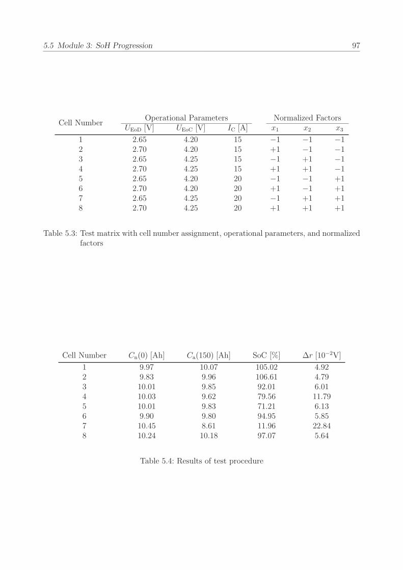
5.5 Module 3: SoH Progression 97
Cell NumberOperational Parameters Normalized Factors
UEoD [V] UEoC [V] IC [A] x1 x2 x3
1 2.65 4.20 15 −1 −1 −12 2.70 4.20 15 +1 −1 −13 2.65 4.25 15 −1 +1 −14 2.70 4.25 15 +1 +1 −15 2.65 4.20 20 −1 −1 +16 2.70 4.20 20 +1 −1 +17 2.65 4.25 20 −1 +1 +18 2.70 4.25 20 +1 +1 +1
Table 5.3: Test matrix with cell number assignment, operational parameters, and normalizedfactors
Cell Number Cn(0) [Ah] Ca(150) [Ah] SoC [%] ∆r [10−2V]
1 9.97 10.07 105.02 4.922 9.83 9.96 106.61 4.793 10.01 9.85 92.01 6.014 10.03 9.62 79.56 11.795 10.01 9.83 71.21 6.136 9.90 9.80 94.95 5.857 10.45 8.61 11.96 22.848 10.24 10.18 97.07 5.64
Table 5.4: Results of test procedure

5.6 Summary and Discussion 98
Ro [mΩ]0.05 0.10 0.15
00
20
40
Figure 5.15: Distribution of initial ohmic resistance
operational parameters but formed a stable SEI film. These cells deteriorate much slowerthan the other tested cells.A graphical overview about the test results is depicted in Figure 5.19. The values at the
tested operational parameter sets correspond to the state of charge after aging.
5.5.3 Discussion
Following the RSM methodology, introduced in Section 2.6.2, the operational parametersare normalized in order to estimate the response surface
x1 =UEoD − 2.675V
0.025V, x2 =
UEoC − 4.225V
0.025V, and x3 =
IC − 17.5A
2.5A. (5.11)
A first-order polynomial relation from Equation (2.33) is applied and parameterized bythe algorithm of least squares. The resulting response is hence obtained as
y = 82.30 + 12.25x1 − 12.15x2 − 13.50x3 . (5.12)
For the maximization of the response, the x1 (end of discharge voltage UEoD) should beincreased. The factors x2 (charge current IC) and x3 (end of charge voltage UEoC) should bedecreased. The greatest impact on the deterioration is realized by factor x3. For practicalpurpose, high charge currents at a high state of charge should be avoided as these may occurduring energy harvesting (recuperation).
5.6 Summary and Discussion
The amount of energy that can be fed to or withdrawn from an accumulator decreases withtime and usage (cycle number). The chemical processes are various and stochastically dis-tributed in time and space. A common simplification is to observe the irreversible change

5.6 Summary and Discussion 99
IC[A]
UEoD[V]
UEoC[V]
2.702.65
4.25
4.20
20
15
x1
x2x3
Figure 5.16: Graphical representation of investigated parameter sub-space, spanned by UEoD,UEoC, and IC
of the ohmic resistance, as this property corresponds to the degree and rate of deteriora-tion [SHWG05]. This phenomenon was observed experimentally by the developed test rigand used for a deterioration estimation algorithm. By using an observer for fault detectionin combination with measured, deterioration-effected physical parameters, a simple but ef-fective method was found that describes the effect of individual operational parameters onthe deterioration progression.Relevant information about tested and non-tested operational parameter sets and their
contribution to the deterioration within the considered sub-space of possible constant op-erational parameters were found. The method is so far validated for constant operationalparameters. The particular contribution of composed loading will need to be investigated infuture research work by taking into account varying additional relevant operational parame-ters, different/additional parameters, etc. The idea is to derive information about switching(varying) operational parameters on the aging and hence further information about varyingoperation. Here, further investigations with decreased maximum charging current can beprocessed, as this factor was found to have the greatest impact on deterioration. By enlarg-ing the database and thus the heuristic knowledge about accumulator aging, the accuracyof the optimal operational parameter set is refined.

5.6 Summary and Discussion 100
UEoD
UEoC
IC
20A
15A
2.65V 2.70V
4.20V
4.25V
1 2
3 4
5 6
7 8
Figure 5.17: Partial sub-space of operational parameters
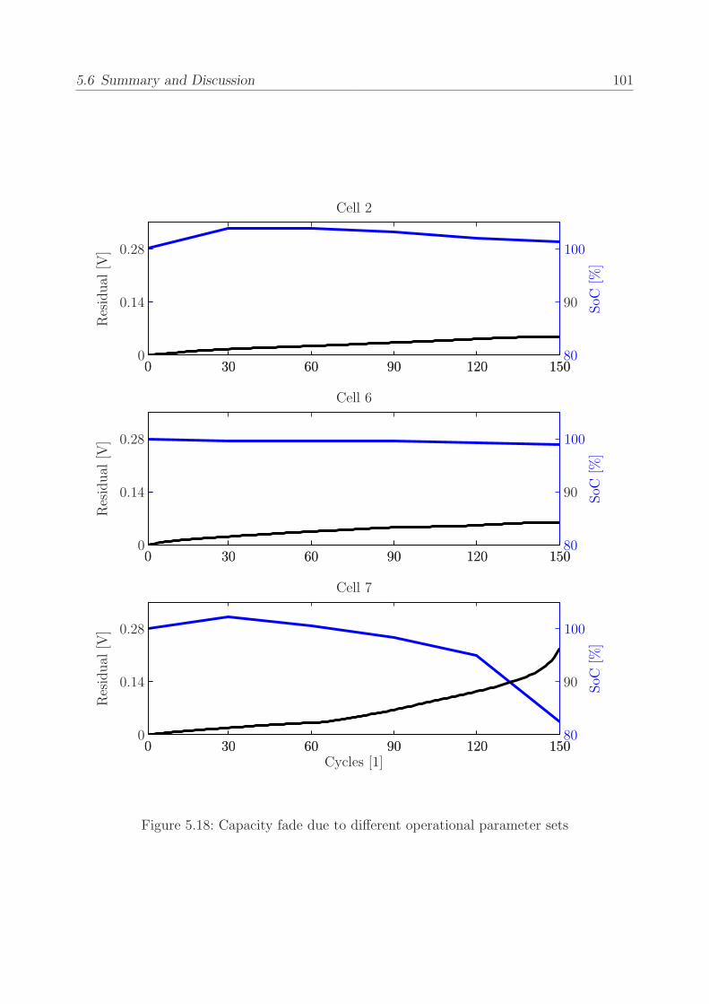
5.6 Summary and Discussion 101
Residual
[V]
Residual
[V]
Residual
[V]
Cycles [1]
SoC
[%]
SoC
[%]
SoC
[%]
0
0
0
0.14
0.14
0.14
0.28
0.28
0.28
100
100
100
80
80
80
00
00
00
3030
3030
3030
6060
6060
6060
90
90
90
90
90
90
90
90
90
120120
120120
120120
150150
150150
150150
Cell 2
Cell 6
Cell 7
Figure 5.18: Capacity fade due to different operational parameter sets

5.6 Summary and Discussion 102
x1
x2
x3
−1
−1 −1
+1
+1
+1
105.02 106.61
92.01 79.56
71.21 94.95
11.96 97.07
Figure 5.19: Partial sub-space of operational parameters

6 Summary and Outlook
The goal of this thesis was to realize and detail the descriptive Safety and Reliability ControlEngineering Concept (SRCE), developed in [RS96, SR97], as there is a demand for an adap-tive compromise between safety and reliability. After introducing reliability-related, relevantdefinitions with a special focus on probabilistic aspects, common ideas on fault detection,fault diagnosis, and fault prognosis are briefly discussed. Based on the SRCE concept andpreliminary works on that [Wol08], the single modules for a reliability-centered operation ofan arbitrary system are developed and discussed in detail.The application of the developed modules constitutes the core of this thesis; application
examples are introduced and discussed in Chapter 4 for a mechanical system failing due tomechanical wear (abrasive wear) and in Chapter 5 for an electro-chemical system failing dueto capacity fade. In Chapter 4, the main focus is on the novel, developed measurement chainand the related evaluation of deterioration-inherent quantities. As the deterioration processis highly non-linear, solely signal-based fault detection and diagnosis approaches are dis-cussed and appropriate, deterioration-specific countermeasures for reliability improvementsare shown. In Chapter 5, a model-based fault detection and diagnosis strategy is developedand novel aspects for appropriate deterioration countermeasures are detailed.
6.1 Summary
The central scientific contributions of this thesis are summarized in the following:
• In order to operate the system within a required (minimum) reliability margin, the de-terioration progression due to prospective operation has to be quantified. In additionwith the actual state-of-deterioration, various scenarios for remaining useful life can bederived and used for appropriate lifetime control strategies. Therefore, traditional andnovel SHM approaches are briefly introduced at the beginning of this thesis. The re-search goes on to describe the so far missing step towards using health information forcontrolling the remaining lifetime by changing specific operation parameters. Based onthe Safety and Reliability Control Engineering concept and preliminary works on that,a novel method, which extends the strategies known from literature, is introduced.The single modules are introduced in detail. In particular, the challenging aspect ofusing deterioration-affected measurands to draw conclusions about the actual state-of-deterioration is detailed. Furthermore, the adaptive, probabilistic-based deteriora-tion model realizes the continuously adaptive, time-variant, probabilistic correlationbetween deterioration-proportional information and the most probable deterioration.From this correlation, information about the remaining useful life can be derived. As adirect consequence of the obtained deterioration estimations, appropriate strategies canbe developed to modify the operation of the systems (by limiting disproportionatelyhigh damaging situations, proposing alternative strategies, etc.).

6.1 Summary 104
• The adaptive probabilistic-based deterioration model realizes the continuously adap-tive, time-variant, probabilistic correlation between deterioration-proportional infor-mation and the most probable deterioration. As a direct consequence of the obtaineddeterioration estimations, appropriate strategies for modifying the operation of the sys-tems (by limiting disproportionately high damaging situations, proposing alternativestrategies, etc.) are derived and proposed.
• The failure due to wear of an industrial machine is investigated. According to theresults of a detailed material analysis, three main tribological mechanisms which leadto failure were identified. For investigation purposes, a test rig which reproduces themain wear effects was presented and a novel measuring chain based on the direct piezo-electric effect for acoustic emission sensing was developed and operated. The FPGAcompatible filter, which realizes the signal analysis, was introduced and an adequatevisualization method was developed to indicate regions and severeness of stochasticallyoccurring wear. Several comparable wear tests were performed for the most typicalmaterial and lubrication combination, and the result was presented. A high correla-tion between the point of failure and the measured deterioration-equivalent signal wasshown. Under normal operation conditions, the deterioration can be estimated withinsufficient probabilistic limits.
• The challenge of estimating the accumulator deterioration and proposing optimal us-age (in terms of phase-specific operational parameters) with the help of independentparameters and non-stationary operation in field usage is demonstrated and solvedby appropriate on-line capable methods. The developed database is realized with aminimum number of required test runs. A common simplification is to observe the irre-versible change of the ohmic resistance, as this property corresponds to the degree andrate of deterioration. This phenomenon was observed experimentally by the developedtest rig and used for a deterioration estimation algorithm. By using an observer forfault detection in combination with measured, deterioration-effected physical param-eters, a simple but effective method was found that describes the effect of individualoperational parameters on the deterioration progression. Relevant information abouttested and non-tested operational parameter sets and their contribution to the dete-rioration within the considered sub-space of possible constant operational parameterswere found. The method is so far validated for constant operational parameters.
This thesis widens the preliminary work by novel aspects of appropriate strategies for ad-dressing and improving systems’ reliability. Additionally, the conceptual ideas of the SRCEconcept are brought into practice for the first time.

6.2 Outlook on Future Work 105
6.2 Outlook on Future Work
Further research should focus on
• the application of the developed algorithms and approaches on further test specimens.The development of a comprehensive data base for both test systems (consideringvariable operational conditions, etc.) is required in order to further detail and validatethe proposed correlations.
• the further improvement of the acoustic emission sensor by developing a housed piezo-electric ceramic in order to reduce the effort of calibration and impedance measurement.The integration of the proposed admittances (piezoelectric ceramic, impedance con-verter, transmission lines, etc.) in the FPGA ensures the signal quality and facilitatesthe correlation of characteristic frequency contents with individual failure modes.
• the variable operation of accumulators, especially depending on the actual state-of-deterioration. It is with a view to this proposed application in particular that thepossible improvement realized by the Response Surface Model-based module 3 can bedemonstrated. The goal is to obtain information about the effect of varying opera-tional parameters on the aging process and, in turn, further information about theeffect varying operation modes have on the lifetime. Here, further investigations withdecreased maximum charging current may be useful, as this factor was found to havethe greatest impact on deterioration.

References
[AB09] D. Astapenko and L. M. Bartlett. System design optimisation involvingphased missions. International Journal of Reliability and Safety, 3(4):331–344, 2009.
[Abe05] R. B. Abernethy. The new Weibull handbook. Reliability & statistical anal-ysis for predicting life, safety, survivability, risk, cost and warranty claims.Abernethy, North Palm Beach, Florida, USA, 4th edition, 2005.
[ACL+01] K. Amine, C. H. Chen, J. Liu, M. Hammond, A. Jansen, D. Dees, I. Bloom,D. Vissers, and G. Henriksen. Factors responsible for impedance rise inhigh power lithium ion batteries. Journal of Power Sources, 97–98:684–687, 2001.
[Arc53] J. F. Archard. Contact and rubbing of flat surfaces. Journal of appliedphysics, 24(8):981–988, 1953.
[AST90] American society for testing and materials. Standard terminology for non-destructive examinations. E 1316-90, 1990.
[Aus96] D. M. Auslander. What is mechatronics? IEEE/ASME Transaction onMechatronics, 1(1):5–9, 1996.
[Ban09] D. Banjevic. Remaining useful life in theory and practice. Metrika, 69(2–3):337–349, 2009.
[Bar05] E. Barsoukov. Impedance spectroscopy. Theory, experiment, and applica-tions. Wiley-Interscience, Hoboken, New Jersey, 2nd edition, 2005.
[BB10] K. G. Budinski and M. K. Budinski. Engineering materials: propertiesand selection. Pearson, Upper Saddle River, NJ u.a., 9. edition, 2010.
[BBB+05] M. Broussely, P. Biensan, F. Bonhomme, P. Blanchard, S. Herreyre,K. Nechev, and R. J. Staniewicz. Main aging mechanisms in Li ion bat-teries. Journal of Power Sources, 146(1-2):90–96, 2005.
[BBHF07] M. Barbezat, A. J. Brunner, C. Huber, and P. Flueler. Integrated ac-tive fiber composite elements: characterization for acoustic emission andacousto-ultrasonics. Journal of Intelligent Material Systems and Struc-tures, 18:515–525, 2007.
[BCL+05] H. Bindner, T. Cronin, P. Lundsager, J. F. Manwell, U. Abdulwahid,and I. Baring-Gould. Lifetime modelling of lead acid batteries. Technicalreport, Risø National Laboratory, 2005.
References 107
[BCS+01] I. Bloom, B. W. Cole, J. J. Sohn, S. A. Jones, E. G. Polzin, V. S. Battaglia,G. L. Henriksen, C. Motloch, R. Richardson, T. Unkelhaeuser, D. Ingersoll,and H. L. Case. An accelerated calendar and cycle life study of Li-ion cells.Journal of Power Sources, 101(2):238–247, 2001.
[BDHH07] G. E. P. Box, N. R. Draper, W. G. Hunter, and J. S. Hunter. Responsesurfaces, mixtures and ridge analyses. Wiley series in probability andstatistics. J. Wiley & Sons, Hoboken, NJ, 2nd edition, 2007.
[Bel98] D. E. Bell. Decision making: descriptive, normative, and prescriptiveinteractions. Cambridge University Press, Cambridge, 1998.
[Bes05] H. W. Bester. Untersuchung des Verschleißes von Riffelblechen - UB050905-1. Technical report, Institute of Product Engineering, Universityof Duisburg-Essen, 2005.
[Bes07] H. W. Bester. Untersuchung des Verschleißes von Riffelblechen - UB230407-1. Technical report, Institute of Product Engineering, Universityof Duisburg-Essen, 2007.
[BFG06] D. Balageas, C. P. Fritzen, and A. Guemes. Structural health monitoring.ISTE, London, 2006.
[BHH05] G. E. P. Box, J. S. Hunter, and W. G. Hunter. Statistics for experimenters:design, innovation, and discovery. Wiley series in probability and statis-tics. Wiley-Interscience, Hoboken, New Jersey, 2nd edition, 2005.
[BIMP04] C. Bonivento, A. Isidori, L. Marconi, and A. Paoli. Implicit fault toler-ant control: Application to induction motors. Automatica, 40(3):355–371,2004.
[Bis94] C. M. Bishop. Neural networks and their applications. Review of scientificinstruments, RSI, 65(6):1803–1832, 1994.
[BKLS06] M. Blanke, M. Kinnaert, J. Lunze, and M. Staroswiecki. Diagnosis andFault-Tolerant Control. Springer-Verlag Berlin Heidelberg, 2nd edition,2006.
[BM91] R. J. Boness and S. L. McBride. Adhesive and abrasive wear studiesusing acoustic emission techniques. Wear: an international journal on thescience and technology of friction, lubrication and wear, 149(1–2):41–53,1991.
[BMFF11] S. Bashash, S. J. Moura, J. C. Forman, and H. K. Fathy. Plug-in hybridelectric vehicle charge pattern optimization for energy cost and batterylongevity. Journal of Power Sources, 196(1):541–549, 2011.
[BMS90] R. J. Boness, S. L McBride, and M. Sobczyk. Wear studies using acousticemission techniques. Tribology International, 23(5):291–295, 1990.

References 108
[BSM+07] R. Bornatico, A. Storti, L. Mandrioli, A. Zappavigna, Y. Guezennec, andG. Rizzoni. NiMH battery characterization and state-of-charge estimationfor HEV applications. ASME Conference Proceedings, 2007(43106):205–214, 2007.
[BSMM05] I. N. Bronstein, K. A. Semendjajew, G. Musiol, and H. Muhlig. Taschen-buch der Mathematik. Harri Deutsch, 6th edition, 2005.
[BW51] G. E. P. Box and K. B. Wilson. On the experimental attainment ofoptimum conditions. Journal of the Royal Statistical Society. Series B(Methodological), 13(1):1–45, 1951.
[CH10] H. Czichos and K.-H. Habig. Tribologie-Handbuch. Tribometrie, Triboma-terialien, Tribotechnik. Vieweg Teubner, Wiesbaden, 3. edition, 2010.
[CFC06] E. Castillo and A. Fernandez-Canteli. A parametric lifetime model forthe prediction of high-cycle fatigue based on stress level and amplitude.Fatigue & Fracture of Engineering Materials & Structures, 29(12):1031–1038, 2006.
[Coi01] D. W. Coit. Cold-standby redundancy optimization for nonrepairable sys-tems. IIE Transactions, 33(6):471–478, 2001.
[CSGR06] Z. Chehab, L. Serrao, Y. Guezennec, and G. Rizzoni. Aging characteri-zation of nickel metal hydride batteries using electrochemical impedancespectroscopy. In ASME International Mechanical Engineering Congressand Exhibition, 2006.
[CT65] J. W. Cooley and J. W. Tukey. An algorithm for the machine calculationof complex fourier series. Mathematicas of Computation, 19:297–301, 1965.
[CV05] J. Chiasson and B. Vairamohan. Estimating the state of charge of a bat-tery. IEEE Transactions on Control Systems Technology, 13(3):465–470,2005.
[DAS06] D. Doerffel and S. Abu Sharkh. A critical review of using the peukertequation for determining the remaining capacity of lead-acid and lithium-ion batteries. Journal of Power Sources, 155(2):395–400, 2006.
[DIN 1313] Fundamental technical standards committee. Quantities (DIN 1313:1998),1998.
[DIN 1319] Fundamental technical standards committee. Fundamentals of metrology- Part 1: Basic terminology (DIN 1319-1), 1995.
[DIN 6344] Tools and clamping devices standards committee. Coated abrasives - grainsize analysis - Part 3: Determination of grain size distribution of microgritsP 240 to P 2500 (ISO 6344-3:1998), 2000.

References 109
[DIN 50321-1] German commission for electrical, electronic and information technologiesof DIN and VDE. piezoelectric properties of ceramic materials and compo-nents - Part 1: Terms and definitions; German version EN 50324-1:2002,2002.
[DIN 50321-3] German commission for electrical, electronic and information technologiesof DIN and VDE. piezoelectric properties of ceramic materials and com-ponents - Part 3: Methods of measurement; high power; German versionEN 50324-3:2002, 2002.
[DIN EN 1330] Materials testing standards committee. Non-destructive testing - Termi-nology DIN EN 1330, 1998-2010.
[DIN EN 60254] German commission for electrical, electronic and information technolo-gies of DIN and VDE. Lead-acid traction batteries - Part 1: General re-quirements and methods of tests (IEC 60254-1:2005); German version EN60254-1:2005, 2006.
[DIN EN 61078] CES-TK 56 dependability, fiabilite et maintenabbilite. Analysis techniquesfor dependability - Reliability block diagram and boolean methods (IEC61078:2006), 2006.
[DS82] S. D. Downing and D. F. Socie. Simple rainflow counting algorithms. Inter-national Journal of Fatigue: Materials, Structures, Components, 4(1):31–40, 1982.
[DS09] K.-U. Dettmann and D. Soffker. Classification of wear phenomena byspecific ultrasonic emission detection for prognostic purposes. In AnnualConference of the Prognostics and Health Management Society, PHM, SanDiego (CA, USA), 2009.
[DW92] S.-H. Dai and M.-O. Wang. Reliability analysis in engineering applications.Van Nostrand Reinhold (NY, USA), 1992.
[EN 13306] Fundamental technical standards committee. Maintenance terminology;trilingual version EN 13306:2010, 2010.
[FCGC01] A. Fei, J. Cui, M. Gerla, and D. Cavendish. A dual-tree scheme for fault-tolerant multicast. In IEEE International Conference on Communications,ICC, volume 3, pp. 690–694, 2001.
[FK01] S. Fouvry and P. Kapsa. An energy description of hard coating wearmechanisms. Surface & coatings technology, 138(2–3):141–148, 2001.
[FK06] C.-P. Fritzen and M. Klinkov. Online force identification with robustobservers. In VDI-Berichte, Band 1941, pp. 303–312, 2006.
[FK09] C.-P. Fritzen and P. Kramer. Self-diagnosis of smart structures based ondynamical properties. Mechanical systems and signal processing (MSSP),23(6):1830–1845, 2009.

References 110
[FLK+03] S. Fouvry, T. Liskiewicz, Ph. Kapsa, S. Hannel, and E. Sauger. An energydescription of wear mechanisms and its applications to oscillating slidingcontacts. Wear: an international journal on the science and technology offriction, lubrication and wear, 255(1):287–298, 2003.
[Fra10] J. Fraden. Handbook of modern sensors. Physics, designs, and applications.AIP Press, Melville, (NY, USA) 3rd edition, 2010.
[Fri05] C.-P. Fritzen. Vibration-based structural health monitoring - concepts andapplications. Key Engineering Materials, Damage Assessment of Struc-tures VI (Volumes 293–294):3–20, 2005.
[Fri10] C.-P. Fritzen. Structural health monitoring, volume 1, chapter 2, pp. 45–224. ISTE Publishing Company, London, U. K., 2010.
[GfT] Gesellschaft fur Tribologie e. V. (GfT). Tribologie Definitionen, Begriffe,Prufung. Technical Report 7, Aachen, 2002.
[GGQ] Deutsche Gesellschaft fur Qualitat e. V. (DGQ). Das Lebensdauernetz -Leitfaden zur grafischen Bestimmung von Zuverlassigkeitskenngroßen derWeibull-Verteilung. Band 17–26. Beuth Verlag; Berlin, Wien, Zurich, 1stedition, 1995.
[GLGP08] F. Garcıa Lorca and M. Garcıa-Posada. Obra completa. Universidad Pon-tificia De Salamanca, Tres Cantos, 2nd edition, 2008.
[GR10] J. Gausemeier and F. Rammig. Entwurf mechatronischer Systeme. Num-ber 272 in HNI-Verlagsschriftenreihe. Heinz-Nixdorf-Institut, Paderborn,2010.
[Gro11] Group Five - Advanced Materials & Technology. Actual list of industrialcells. online, http://kokamdirect.com/, July 2011.
[Gue08] R. M. Guedes. Creep and fatigue lifetime prediction of polymer matrixcomposites based on simple cumulative damage laws. Composites, PartA: Applied Science and Manufacturing, 39(11):1716–1725, 2008.
[HDS10] D. Hockmann, K.-U. Dettmann, and D. Soffker. Merkmalsbasierte Zus-tandsbeschreibung werkstoffseitiger Verschleißzustande. In 3. Tagung desDVM-Arbeitskreises: Zuverlassigkeit mechatronischer und adaptronischerSysteme, pp. 93–102, Darmstadt (Germany), 2010.
[Hen55] D. L. Henry. A theory of fatigue-damage accumulation in steel. Transac-tion of the ASME, 77(6):913–917, 1955.
[HH86] W. Hwang and K. S. Han. Cumulative damage models and multi-stressfatigue life prediction. Composite Materials, 20(2):125–153, 1986.

References 111
[HH09] L. Hollmotz and M. Hackmann. Lithium-Ionen Batterien: Anforderung-en und Risiken beim Einsatz aus dem Blickwinkel der Kraftfahrzeug-sicherheit. Innovativer Kfz-Insassen- und Partnerschutz - VDI-TagungFahrzeugsicherheit, 7:101–114, 2009.
[HK91] J. Hanchi and B. E. Klamecki. Acoustic emission monitoring of the wearprocess. Wear: an international journal on the science and technology offriction, lubrication and wear, 145(1):1–27, 1991.
[Hol79] J. O. Holmen. Fatigue of concrete by constant and variable amplitudeloading. University of Trondheim, Institute of Technology, Norway, 1979.
[Hol82] J. O. Holmen. Fatigue of concrete by constant and variable amplitudeloading. In S. P. Shah, editor, Fatigue of concrete structures, volume 75,pp. 71–110, 1982.
[HS09] F. Heidtmann and D. Soffker. Virtual sensors for diagnosis and prognosispurposes in the context of elastic mechanical structures. Sensors Journal,IEEE, 9(11):1577–1588, 2009.
[HWHB09] S. O. Han, K. Wolf, H. Hanselka, and T. Bein. Sensitivity evaluation ofadaptive systems with respect to scattering design and environment pa-rameters. In VDI-Berichte 2065, pp. 145–155. Fraunhofer-Institut fur Be-triebsfestigkeit und Systemzuverlassigkeit (LBF), Darmstadt, VDI-Verlag,2009.
[IEC 60050-191] German commission for electrical, electronic and information technologiesof DIN and VDE. International electrotechnical vocabulary - chapter 191:Dependability and quality of service (IEC 50(191):1990), 1994.
[IEC 60050-486] German commission for electrical, electronic and information technologiesof DIN and VDE. International electrotechnical vocabulary - part 486:Secondary cells and batteries (IEC 50(486):1991), 1994.
[Ike90] T. Ikeda. Fundamentals of piezoelectricity. Oxford science publications.Oxford University Press, 1990.
[Ise99] R. Isermann. Mechatronische Systeme: Grundlagen. Springer, Berlin[u. a.], 1999.
[Ise06] R. Isermann. Fault diagnosis systems: an introduction from fault detectionto fault tolerance. Springer Berlin Heidelberg, 2006.
[IVA90] Journal of Vibration and Acoustics. American Society of Mechanical En-gineers (ASME) and American Institute of Physics (AIP), since 1990.
[JBS+04] H. Janocha, S. Butzmann, H. D. Stolting, W. Backe, and A. Klein. Actu-ators: basics and applications. Springer, Berlin, 1st edition, 2004.

References 112
[Jon09] K. Jonas. Online-Alterungsdiagnose und belastungsabhangige Lebensdau-erprognose von Polymerelektrolyt-Brennstoffzellen. Dissertation, Techni-sche Universitat Dresden, Professur fur Energiesystemtechnik und War-mewirtschaft, Dusseldorf, VDI-Verlag, 2009.
[JW06] A. Jossen and W. Weydanz. Moderne Akkumulatoren richtig einsetzen.Reichardt, Untermeitingen, 1st edition, 2006.
[Kal60] R. E. Kalman. On the general theory of control systems. IRE Transactionson Automatic Control, 4(3):481–493, 1960.
[Kas06] K. Kashi. Development of a Fault Diagnosis System for an Active RollControl System using Observers and Virtual Sensors. Dissertation, Chairof Dynamics and Control (SRS), Department of Mechanical Engineering,Faculty of Engineering Sciences, University of Duisburg-Essen, Duisburg,Germany, 2006.
[KBSM09] M. Keller, P. Birke, M. Schiemann, and U. Mohrstadt. Lithium ion batterydevelopment for hybrid and electrical vehicle. ATZ-Elektronik, 4(2):16–23,2009.
[Kha02] H. K. Khalil. Nonlinear systems. Prentice Hall, Upper Saddle River, NJ,3rd edition, 2002.
[Kim10] I.-S. Kim. A technique for estimating the state of health of lithium bat-teries through a dual-sliding-mode observer. IEEE Transactions on PowerElectronics, 25(4):1013–1022, 2010.
[KRC+10] U. Krupp, I. Roth, H. J. Christ, M. Kubbeler, and C.-P. Fritzen. Insitu SEM observation and analysis of martensitic transformation duringshort fatigue crack propagation in metastable austenitic steel. AdvancedEngineering Materials, 12(4):255–261, 2010.
[LLO11] H. Li, J. Liu, and J. Ou. Seismic response control of a cable-stayed bridgeusing negative stiffness dampers. Structural Control and Health Monitor-ing, 18:265–288, 2011.
[LMWK01] J. Li, E. Murphy, J. Winnick, and P. A. Kohl. Studies on the cycle lifeof commercial lithium ion batteries during rapid charge-discharge cycling.Journal of Power Sources, 102(1–2):294–301, 2001.
[LSSM10] A. Ling, C. Shantz, S. Sankararaman, and S. Mahadevan. Stochastic char-acterization and update of fatigue loading for mechanical damage progno-sis. In Annual Conference of the Prognostics and Health ManagementSociety, 2010.
[Lue64] D. G. Luenberger. Observing the state of a linear system. IEEE Transac-tions on Military Electronics, 8(2):74–80, 1964.

References 113
[Lun08] J. Lunze. Regelungstechnik 2: Mehrgroßensysteme, Digitale Regelung.Springer-Verlag Berlin Heidelberg, 5th edition, 2008.
[LYY93] S. Lingard, C. W. Yu, and C. F. Yau. Sliding wear studies using acousticemission. Wear: an international journal on the science and technology offriction, lubrication and wear, 162–164(1):597–604, 1993.
[ME68] M. Matsuishi and T. Endo. Fatigue of metals subjected to varying stress.Japan Society of Mechanical Engineering, 1968.
[MEC02] Q. W. Meeker, L. A. Escobar, and V. Chan. Using accelerated tests topredict service life in highly variable environments, chapter 19, pp. 396–413. American Chemical Society, 2002.
[MFSF09] S. J. Moura, J. Forman, J. L. Stein, and H. K. Fathy. Control of filmgrowth in lithium ion battery packs via switches. 2nd Annual DynamicSystems and Control Conference, DSCC, 2009.
[MIL-HDBK] Military handbook - Reliability prediction of electronic equipment MIL-HDBK-217F. U. S. Department of Defense. Technical report, 1991.
[MIL-STD] Military handbook - Standard practice for system safety MIL-STD-882D.U. S. Department of Defense. Technical report, 2000.
[MIL-NSWC] Handbook of reliability prediction procedures for mechanical equipmentNSWC-06. Logistics technology support group, carderock division, navalsurface warfare center (CDNSWC). Technical report, 2006.
[Min45] M. A. Miner. Cumulative damage in fatigue. Journal of Applied Mechan-ics, 12(3):159–164, 1945.
[MM10] H. Ma and W. Q. Meeker. Strategy for planning accelerated life tests withsmall sample sizes. IEEE Transactions on Reliability, 59(4):610–619, 2010.
[MMS+03] N. K. Myshkin, L. V. Markova, M. S. Semenyuk, H. Kong, H.-G. Han, andE.-S. Yoon. Wear. 14th International Conference on Wear of Materials,255(7-12):1270–1275, 2003.
[Mon09] D. C. Montgomery. Design and analysis of experiments. Wiley, Hobo-ken, NJ, 7th edition, 2009.
[Mor05] C. Moraga. Data Driven Fuzzy Modelling with Neural Networks, volume179 of Studies in Fuzziness and Soft Computing, chapter 1, pp. 153–164.Springer Berlin Heidelberg, 2005.
[MS54] S. M. Marco and W. L. Starkey. A concept of fatigue damage. Transactionof the ASME, 76(4):626–662, 1954.
[MvKM05] R. K. Miller, E. v. Kill, and P. O. Moore. Acoustic emission testing.American Society for Nondestructive Testing, 2005.

References 114
[MXJ04] D. N. P. Murthy, M. Xie, and R. Jiang. Weibull models. New York: Wiley,2004.
[MZD03] B. Moreno, J. Zapatero, and J. Domınguez. An experimental analysisof fatigue crack growth under random loading. International Journal ofFatigue, 25(7):597–608, 2003.
[Nac05] J. A. Nachlas. Reliability engineering. probabilistic models and mainte-nance methods. Taylor & Francis, Boca Raton u. a., 2005.
[Nel01] O. Nelles. Nonlinear System Identification. Springer, Berlin, 2001.
[NF99] M. Nagode and M. Fajdiga. The influence of variable operating conditionsupon the general multi-modal weibull distribution. Reliability engineering& system safety, 64(3):383, 1999.
[Oza09] K. Ozawa. Lithium ion rechargeable batteries. Wiley-VCH, 2009.
[Ozb10] M. Ozbek. Modeling, Simulation, and Concept Studies of a Fuel Cell Hy-brid Electric Vehicle Powertrain. Dissertation, Chair of Dynamics andControl (SRS), Department of Mechanical Engineering, Faculty of Engi-neering Sciences, University of Duisburg-Essen, Duisburg, Germany, 2010.
[Pal24] A. Palmgren. Die Lebensdauer von Kugellagern. VDI-Z, 68(14):339–341,1924.
[PFKN09] C. Papadimitriou, C. P. Fritzen, P. Kraemer, and E. Ntotsios. Fatiguelifetime estimation in structures using ambient vibration measurements. InM. Papadrakakis, N. D. Lagaros, and M. Fragiadakis, editors, ECCOMASThematic Conference on Computational Methods in Structural Dynamicsand Earthquake Engineering (COMPDYN), 2009.
[PI11] PI Ceramic. Typical parameters of piezoelectric ceramics. Internet re-source http://www.piceramic.com/, 2011.
[Pic07] N. Picciano. Battery aging and characterization of nickel metal hydrideand lead acid batteries. Master’s thesis, Center for Automotive Research,Department of Mechanical Engineering, Ohio State University, 2007.
[Poh03] J. Pohl. Zerstorungsfreie Charakterisierung adaptiver CFK-Piezokeramik-Verbunde: konventionelle Verfahren und health monitoring. Habilitation,Fakltat fur Maschinenbau, Institut fur Werkstoff- und Fugetechnik, Otto-von-Guericke-Universitat Magdeburg, 2003.
[Rai09] G. B. Raines, editor. Electric vehicles. technology, research, and develop-ment. Nova Science Publishers Inc, New York, 2009.
[Ram03] P. Ramadass. Mathematical modeling of the capacity fade of Li-ion cells.Journal of Power Sources, 123(2):230–240, 2003.
References 115
[Ran47] J. E. Randles. Kinetics of rapid electrode reactions. Discussions Of TheFaraday Society, 1:11–19, 1947.
[RBM+10] J. Remmlinger, M. Buchholz, M. Meiler, P. Bernreuter, and K. Diet-mayer. State-of-health monitoring of lithium-ion batteries in electric vehi-cles by on-board internal resistance estimation. Journal of Power Sources,196(12):5357–5363, 2010.
[RDS10] J. Ravelin, K.-U. Dettmann, and D. Soffker. Examinations classifying wearstates using signal-based approaches. In Gordon Reserarch Conference onTribology - Challenges at the Buried Interface, 2010.
[RH04] M. Rausand and A. Høyland. System reliability theory. Models, statisticalmethods, and applications. Wiley series in probability and statistics appliedprobability and statistics. Wiley-Interscience, Hoboken, NJ, 2nd edition,2004.
[RHG+04] P. Ramadass, B. Haran, P. M. Gomadam, R. White, and B. N. Popov.Development of first principles capacity fade model for Li-ion cells. Journalof The Electrochemical Society, 151(2):A196–A203, 2004.
[RLB+01] A. G. Ritchie, B. Lakeman, P. Burr, P. Carter, P. N. Bames, and P. Bowles.Battery degradation and ageing, chapter 5, pp. 523–527. New York: KluwerAcademic/Plenum Publishers, 2001.
[RMC+07] M. R. Raupach, G. Marland, P. Ciais, C. Le Quere, J. G. Canadell,G. Klepper, and C. B. Field. Global and regional drivers of accelerat-ing CO2 emissions. In Proceedings of the National Academy of Sciences ofthe United States of America, volume 104, pp. 10288–10293, 2007.
[RS96] U. K. Rakowsky and D. Soffker. Verknupfung von Methoden derRegelungstheorie und der Technischen Zuverlassigkeit zur Modellierungdynamischer Systeme. VDI Berichte, 1282:753–763, 1996.
[Run10] A. Runge. Modellierung der Lebensdauer von Systemen. Master’s thesis,Institut fur Mathematik, Universitat Potsdam, 2010.
[San08] M. Sander. Sicherheit und Betriebsfestigkeit von Maschinen und Anlagen.Konzepte und Methoden zur Lebensdauervorhersage. Springer, Berlin u. a.,2008.
[SCGR05] L. Serrao, Z. Chehab, Y. Guezennee, and G. Rizzoni. An aging model ofNi-MH batteries for hybrid electric vehicles. pp. 78–85, 2005.
[SCW+09] M. Sternad, M. Cifrain, D. Watzenig, G. Brasseur, and M. Winter. Con-dition monitoring of lithium-ion batteries for electric and hybrid electricvehicles. e & i. Elektrotechnik und Informationstechnik, 126(5):186–193,2009.

References 116
[SFH+04] H. Sohn, C. R. Farrar, F. M. Hemez, D. D. Shunk, S. W. Stinemates,B. R. Nadler, and J. J. Czarnecki. A Review of Structural Health Monitor-ing Literature form 1996-2001. Report. Los Alamos National Laboratoryreport LA-13976-MS (2004).
[SG08] B. Saha and K. Goebel. Uncertainty management for diagnostics andprognostics of batteries using bayesian techniques. pp. 1–8, 2008.
[SG09] B. Saha and K. Goebel. Modeling Li-ion battery capacity depletion in aparticle filtering framework. In Annual Conference of the Prognostics andHealth Management Society, PHM, 2009.
[SGPC09] B. Saha, K. Goebel, S. Poll, and J. Christophersen. Prognostics methodsfor battery health monitoring using a bayesian framework. IEEE Trans-actions on Instrumentation and Measurement, 58(2):291–296, 2009.
[SH87] T. Shimokawa and Y. Hamaguchi. Statistical evaluation of fatigue lifeand fatigue strength in circular-hole notched specimens of a carbon eight-harness-satin/epoxy laminate. Statistical research on fatigue and fracture,A88-51351 22–39:159–176, 1987.
[Shu02] P. J. Shull. Nondestructive evaluation: theory, techniques, and applica-tions. Mechanical engineering; 142. Marcel Dekker, Inc., New York, Basel,2002.
[SHWG05] A. T. Stamps, C. E. Holland, R. E. White, and E. P. Gatzke. Analysis ofcapacity fade in a lithium ion battery. Journal of Power Sources, 150:229–239, 2005.
[SLWW02] J. Y. Song, H. H. Lee, Y. Y. Wang, and C. C. Wan. Two- and three-electrode impedance spectroscopy of lithium-ion batteries. Journal ofPower Sources, 111(2):255–267, 2002.
[SR97] D. Soffker and U. K. Rakowsky. Perspectives of monitoring and con-trol of vibrating structures by combining new methods of fault detectionwith new approaches of reliability engineering. In 12th ASME Conferenceon Reliability, Stress Analysis and Failure Prevention, pp. 671–682, April1997.
[SRA+08] A. Saltelli, M. Ratto, T. Andres, F. Campolongo, J. Cariboni, D. Gatelli,M. Saisana, and S. Tarantola. Global sensitivity analysis. The primer.John Wiley & Sons, Chichester, England; Hoboken, NJ, 2008.
[SSB+07] J. Schiffer, D. U. Sauer, H. Bindner, T. Cronin, P. Lundsager, andR. Kaiser. Model prediction for ranking lead-acid batteries according toexpected lifetime in renewable energy systems and autonomous power-supply systems. Journal of Power Sources - 10th European Lead BatteryConference, 168(1):66–78, 2007.

References 117
[SW08] D. U. Sauer and H. Wenzl. Comparison of different approaches for life-time prediction of electrochemical systems - using lead-acid batteries asexample. Journal of Power Sources, 176(2):534–546, 2008.
[Sye10] A. Syed. Limitations of Norris-Landzberg equation and application ofdamage accumulation based methodology for estimating acceleration fac-tors for pb free solders. In 11th International Conference on Thermal,Mechanical Multi-Physics Simulation, and Experiments in Microelectron-ics and Microsystems, (EuroSimE), pp. 1–11, 2010.
[TEKP10] J. Tichy, J. Erhart, E. Kittinger, and J. Prıvratska. Fundamentalsof Piezoelectric Sensorics. Mechanical, Dielectric, and ThermodynamicalProperties of Piezoelectric Materials. Springer-Verlag, Berlin, Heidelberg,2010.
[TSG08] U. Tietze, C. Schenk, and E. Gamm. Electronic circuits: Handbook fordesign and application. Springer, Berlin, 2nd edition, 2008.
[VDI 3452] VDI/VDE-society measurement and automation. Safety terms for automa-tion systems - Qualitative terms and definitions VDI/VDE 3542 Blatt 1,2000.
[VDI 4008] VDI society product and process design. Conditions and applicational pref-erences of reliability analyses VDI 4008, 1998.
[Vez10] A. Vezzini. Elektrofahrzeuge: Mobilitat und erneuerbare Energie. Physikin unserer Zeit, 41:36–42, 2010.
[VNW+05] J. Vetter, P. Novak, M. R. Wagner, C. Veit, K.-C. Moller, J. O. Besenhard,M. Winter, M. Wohlfahrt-Mehrens, C. Vogler, and A. Hammouche. Ageingmechanisms in lithium-ion batteries. Journal of Power Sources, 147(1–2):269–281, 2005.
[VPB07] A. Vasebi, M. Partovibakhsh, and S. M. Taghi Bathaee. A novel combinedbattery model for state-of-charge estimation in lead-acid batteries basedon extended Kalman filter for hybrid electric vehicle applications. Journalof Power Sources, 174(1):30–40, 2007.
[WDB04] K. Worden and J. M. Dulieu-Barton. An overview of intelligent faultdetection in systems and structures. Structural Health Monitoring, SHM,3(1):85–98, 2004.
[Wei51] W. Weibull. A statistical distribution function of wide applicability. Jour-nal of Applied Mechanics, 18(3):239–297, 1951.
[Whi87] R. M. White. A sensor classification scheme. Ferroelectrics and FrequencyControl, IEEE Transactions on Ultrasonics, 34(2):124–126, 1987.
[WM04] M. Wohlfahrt-Mehrens. Aging mechanisms of lithium cathode materials.Journal of Power Sources, 127(1–2):58–64, 2004.

References 118
[Woh70] A. Wohler. Uber die Festigkeitsversuche mit Eisen und Stahl. Zeitschriftfur Bauwesen XX, 20:73–106, 1870.
[Wol08] K. Wolters. Formalismen, Simulation und Potenziale eines nutzungsopti-mierenden Zuverlassigkeitskonzepts. Dissertation, Chair of Dynamics andControl (SRS), Department of Mechanical Engineering, Faculty of Engi-neering Sciences, University of Duisburg-Essen, Duisburg, Germany, 2008.
[WS04] K. Wolters and D. Soffker. The SRCE concept - a probabilistic avoidanceof failures. In Proceedings of the IAR Annual Meeting, pp. 229–234, 2004.
[WS05] K. Wolters and D. Soffker. The potential of the safety and reliabilitycontrol engineering concept as framework for reliability based utilizationstrategies. In F. K. Chang, editor, Proceedings of the 5th InternationalWorkshop on Structural Health Monitoring, SHM, pp. 1353–1360, 2005.
[WZX09] X. Wei, B. Zhu, and W. Xu. Internal resistance identification in vehiclepower lithium-ion battery and application in lifetime evaluation. In Pro-ceedings of the 2009 International Conference on Measuring Technologyand Mechatronics Automation, volume 3, pp. 388–392, Washington, D.C.,USA, 2009.
[YPL96] P. Young, S. Parkinson, and M. Lees. Simplicity out of complexity inenvironmental modelling - Occam’s razor revisited. Journal of appliedstatistics, 23(2–3):165–210, 1996.
[ZHD+00] D. Zhang, B. S. Haran, A. Durairajan, R. E. White, Y. Podrazhansky, andB. N. Popov. Studies on capacity fade of lithium-ion batteries. Journal ofPower Sources, 91(2):122–129, 2000.
[ZW08] Q. Zhang and R. E. White. Capacity fade analysis of a lithium ion cell.Journal of Power Sources, 179(2):793–798, 2008.
Im Rahmen von Forschungs- und Projektarbeiten im Lehrstuhl SRS wurden vonDr.-Ing. Kai-Uwe Dettmann und Univ.-Prof. Dr.-Ing. Dirk Soffker die nachstehendenStudien-, Diplom-, Bachelor-, Projekt- und Masterarbeiten inhaltlich betreut, wobei Be-standteile und Ergebnisse aus den Forschungs- und Projektarbeiten sowie den studentisch-en Qualifikationsarbeiten wechselseitig in die jeweiligen Arbeiten und somit auch in diesePromotionsarbeit eingeflossen sind.
[Don08] F. Dong. Design and comparison of nonlinear control methods for a hy-draulic servo system with simulation study of force tracking. Master thesis,Chair of Dynamics and Control (SRS), Department of Mechanical Engi-neering, Faculty of Engineering Sciences, University of Duisburg-Essen,Duisburg, Germany, 2008.

References 119
[EJ09] B. Egenolf Jonkmanns. Grundlagenbetrachtung fur die Erfassung ver-schleißcharakteristischer Ultraschallsignale mittels geeigneter Piezokera-miken. Master thesis, Chair of Dynamics and Control (SRS), Departmentof Mechanical Engineering, Faculty of Engineering Sciences, University ofDuisburg-Essen, Duisburg, Germany, 2009.
[Esc09] S. Esch. Signalanalyse von Ultraschallsignalen zur Extraktion von Schadi-gungsphanomenen. Projektarbeit, Chair of Dynamics and Control (SRS),Department of Mechanical Engineering, Faculty of Engineering Sciences,University of Duisburg-Essen, Duisburg, Germany, 2009.
[Jin11] X. Jin. Parametrierung von Akkumulatoralterungsmodellen mittels exper-imentell bestimmter Kenngroßen. Diplomarbeit, Chair of Dynamics andControl (SRS), Department of Mechanical Engineering, Faculty of Engi-neering Sciences, University of Duisburg-Essen, Duisburg, Germany, 2011.
[Rav11] J. Ravelin. Klassifikation von Schleißblechzustanden anhand der auftre-tenden Verschleißerscheinungsformen. Bachelor thesis, Chair of Dynamicsand Control (SRS), Department of Mechanical Engineering, Faculty ofEngineering Sciences, University of Duisburg-Essen, Duisburg, Germany,2011.
[Sac10] O. Sacher. Programmierung von Auswertealgorithmen auf einer FPGA-Messdatenanalysehardware mittels Matlab/Simulink und toolboxen. Stu-dienarbeit, Chair of Dynamics and Control (SRS), Department of Mechan-ical Engineering, Faculty of Engineering Sciences, University of Duisburg-Essen, Duisburg, Germany, 2010.
[Xu10] X. Xu. Simulation von Batterielebensdauermodellen. Diplomarbeit, Chairof Dynamics and Control (SRS), Department of Mechanical Engineering,Faculty of Engineering Sciences, University of Duisburg-Essen, Duisburg,Germany, 2010.
[Zha08] M. Zhang. Identification of time-invariant discrete and continuous math-ematical systems in Matlab/Simulink. Master thesis, Chair of Dynamicsand Control (SRS), Department of Mechanical Engineering, Faculty ofEngineering Sciences, University of Duisburg-Essen, Duisburg, Germany,2008.
![Probabilistic-based method for realizing safe and reliable … · 2012. 1. 24. · the probability of failure or the degradation of the functioning of an item [IEC 60050-191]. Consequently,](https://img.dokumen.tips/doc/110x75/612e8b231ecc51586942e164/probabilistic-based-method-for-realizing-safe-and-reliable-2012-1-24-the-probability.jpg)