Probabilistic Analysis probabilistic analysis methods, including the first and second-order reliability methods, Monte

Carlo simulation, Importance sampling, Latin Hypercube sampling, and stochastic expansions

stochastic finite element method

Solution Techniques for Structural Reliability Reliability analysis evaluates the probability of structural failure by determining whether the

limit-state functions are exceeded.

However, reliability analysis is not limited to calculation of the probability of failure.

Evaluation of various statistical properties, such as probability distribution functions and

confidence intervals of structural responses, plays an important role in reliability analysis.

Structural Reliability Assessment If, when a structure exceeds a specific limit, the structure is unable to perform as required, then

the specific limit is called a limit-state.

The structure will be considered unreliable if the failure probability of the structure limit-state

exceeds the required value. For most structures, the limit-state can be divided into two

categories:

Ultimate limit-states are related to a structural collapse of part or all of the structure. Examples of

the most common ultimate limit-states are corrosion, fatigue, deterioration, fire, plastic

mechanism, progressive collapse, fracture, etc. Such a limit-state should have a very low

probability of occurrence, since it may risk the loss of life and major financial losses.

Serviceability limit-states are related to disruption of the normal use of the structures. Examples

of serviceability limit-states are excessive deflection, excessive vibration, drainage, leakage,

local damage, etc. Since there is less danger than in the case of ultimate limit-states, a higher

probability of occurrence may be tolerated in such limit-states. However, people may not use

structures that yield too much deflections, vibrations, etc.

Generally, the limit-state indicates the margin of safety between the resistance and the load of

structures. The limit-state function, g(.) , and probability of failure, Pf , can be defined as

where R is the resistance and S is the loading of the system. Both R(.) and S(.) are functions of

random variables X. The notation g(.) < 0 denotes the failure region. Likewise, g(.) = 0 and g(.) >

0 indicate the failure surface and safe region, respectively.

The mean and standard deviation of the limit-state, g(.) , can be determined from the elementary

definition of the mean and variance. The mean of g(.) is

where, R and S are the means of R and S, respectively. And the standard deviation of g(.) is

The safety index or reliability index, β, is defined as

If the resistance and the loading are uncorrelated ( RS =0 ), the safety index becomes

The safety index indicates the distance of the mean margin of safety from g(.) = 0.

Figure shows a geometrical illustration of the safety index in a one dimensional case.

The shaded area identifies the probability of failure.

Thus, the probability density function of the limit-state function in this case is

The probability of failure is

When the normally distributed g(.) = 0, the probability of failure is computed as

where (.) is the standard normal cumulative distribution function.

For the multidimensional case, the generalization Equation becomes

Another well-known definition of reliability analysis is the safety factor, F:

Failure occurs when F = 1, and if the safety factors are assumed to be normally distributed, the

safety index is given by

Example 3.1 The figure below shows a simply-supported beam loaded at the midpoint by a concentrated force

P. The length of the beam is L, and the bending moment capacity at any point along the beam is

WT, where W is the plastic section modulus and T is the yield stress.

All four random variables P, L, W, and T are assumed to be independent normal distributions.

The mean values of P, L, W, and T are 10 kN, 8 m, 100×10-6

m3, and 600×10

3 kN/m2

respectively.

The standard deviations of P, L, W, and T are 2 kN, 0.1 m, 2 ×10-5

m3, and 10

5 kN/m

2,

respectively.

The limit-state function is given as

Solve for the safety index, β, and the probability of failure, Pf, for this problem

Solution From the given limit-state,

Using Equation

the safety index is calculated as

Historical Developments of Probabilistic Analysis

First- and Second-order Reliability Method

Due to the curse of dimensionality in the probability-of-failure calculation, numerous methods

are used to simplify the numerical treatment of the integration process.

The Taylor series expansion is often used to linearize the limit-state g(X) = 0.

the first- or second-order Taylor series expansion is used to estimate reliability.

These methods are referred to as the First Order Second Moment (FOSM) and Second Order

Second Moment (SOSM) methods, respectively.

The safety index approach to reliability analysis is actually a mathematical optimization problem

for finding the point on the structural response surface (limit-state approximation) that has the

shortest distance from the origin to the surface in the standard normal space.

In the transformation procedure, the design vector X is transformed into the vector of

standardized, independent Gaussian variables, U.

it makes the most significant contribution to the nominal failure probability Pf = (-β), this

design point is called the Most Probable failure Point (MPP).

Different approximate response surfaces g(U)=0 correspond to different methods for failure

probability calculations.

If the response surface is approached by a first-order approximation at the MPP, the method is

called the first-order reliability method (FORM);

if the response surface is approached by a secondorder approximation at the MPP, the method is

called the second-order reliability method (SORM).

In FORM, the limit-state is approximated by a tangent plane at the MPP.

Stochastic Expansions

The purpose of the stochastic expansion is to better represent uncertainties of systems by

introducing a series of polynomials aimed at characterizing the stochastic system being

investigated.

Monte Carlo Simulation (MCS)

The Monte Carlo method consists of digital generation of random variables and functions,

statistical analysis of trial outputs, and variable reduction techniques.

The computation procedure of MCS is quite simple:

1) Select a distribution type for the random variable

2) Generate a sampling set from the distribution

3) Conduct simulations using the generated sampling set

Simple random sampling is a possible tool to measure the arbitrarily selected area S from the unit

square plane (Figure a).

The area can be approximately calculated by the ratio of m/n where n is the number of sampling

points and m is the number of points that fall inside the area S.

The exact area is geometrically calculated as 0.47.

The obtained area, determined by using 50 random samples based on uniform distribution, yields

0.42, which means that 21 points appear inside the area S. It is obvious that the distribution type

and the boundary limit are decisive parts of the sampling procedure.

When the sampling scheme is aimed at the center of the unit area, a distorted result might be

obtained, as shown in Figure b. In this case, 47 points appear inside, and the ratio 47/50 yields

the overestimated area of 0.94.

Another important factor in the accuracy of the sampling method is the number of sampling

points. When the number of sampling points is increased to 500 uniformly distributed points, the

accurate result of 0.476 is obtained (Figure d).

The same idea can be extended to the analysis of structural reliability.

First, the sampling set of the corresponding random variables are generated according to the

probability density functions.

Next, we set the mathematical model of g(.) , namely the limit-state, which can determine

failures for the drawing samples of the random variables.

Then, after conducting simulations using the generated sampling set, we can easily obtain the

probabilistic characteristics of the response of the structures. In the above example, “Hit or Miss”

of the area S represents the function g(.) . If the limit-state function g(.) is violated, the structure

or structural element has “failed.”

The trial is repeated many times to guarantee convergence of the statistical results. In each trial,

sample values can be digitally generated and analyzed. If N trials are conducted, the probability

of failure is given approximately by

where Nf is the number of trials for which g(.) is violated out of the N experiments conducted.

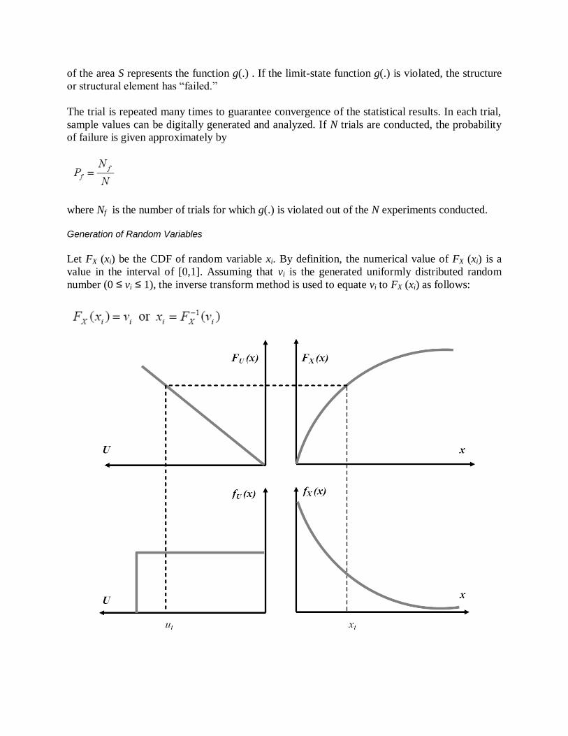
Generation of Random Variables

Let FX (xi) be the CDF of random variable xi. By definition, the numerical value of FX (xi) is a

value in the interval of [0,1]. Assuming that vi is the generated uniformly distributed random

number (0 ≤ vi ≤ 1), the inverse transform method is used to equate vi to FX (xi) as follows:

the approximate probability of failure is

but it is not the most efficient, especially in complex systems.

or

where I[X ] is an indicator function, which equals 1 if [ g(X ) ≤ 0 ] is “true” and 0 if [ g(X ) ≤ 0 ]

is “false.”

Hence,

and its variance is

In order to evaluate Pf by the Monte Carlo method, a sample value for basic variable xi with a

cumulative distribution FX (xi) must be drawn. The inverse transform method can be used to

obtain the random variate, in which a uniformly distributed random number ui (0 ≤ ui ≤ 1) is

generated and equated to FX (xi), i.e.,

Hence, independent random numbers u1,u2 ,...,un are drawn from the density fx (xi ) , and the

estimate of Pf is obtained:

and the sample variance is given as

Example 3.3

Estimate the safety index β of Example 3.1 by using the MCS method with the same limit-state

function, mean values, standard deviations, and distributions of the random variables.

As shown in the table, the MCS results are converged to three digits after 200,000 runs (β = 2.85,

Pf = 0.0021).

In structural reliability analysis, where the probability of failure is generally relatively small, the

direct (crude) Monte Carlo simulation procedure becomes inefficient. The importance sampling

method is a modification of Monte Carlo simulation in which the simulation is biased for greater

efficiency.

In importance sampling, the sampling is done primarily in the tail of the distribution, rather than

spreading it out evenly, in order to ensure that sufficient simulated failures occur.

Latin Hypercube Sampling (LHS)

Stochastic Finite Element Method (SFEM)

The FEM is used in various fields of structural engineering and deals with deterministic

parameters, despite the fact that the problems to which they are applied involve uncertainties of

considerable degree.

When there are requirements for analyzing stochastic behavior of structural systems with random

parameters, one of the applicable solutions is the Stochastic Finite Element Method (SFEM).

SFEM, which combines probability theory with deterministic FEM procedures, is becoming

robust enough to allow engineers to estimate the risk of structural systems.

Deterministic FEM in linear elasticity yields Ku = f. SFEM is an extension of deterministic FEM

for considering the fluctuation of structural properties, loads, and responses of stochastic

systems.

SFEM, which combines probability theory and statistics within FEM, provides an efficient

alternative to time-costly MCS and allows engineers to estimate the risk of structural designs.

The main difference between SFEM and deterministic FEM is in the incorporation of

randomness into the formulation.

The global stiffness matrix can be split into two parts: the deterministic part, K0 , and the

fluctuation (uncertainty) part, K .

where u is the random response of the structure and f is the possibly random excitation of the

system.

There are four typical methods for formulating the fluctuation part of the SFEM procedure:

perturbation method,

Neumann expansion method,

weighted integral method, and

spectral stochastic finite element method.

Basic Formulations of perturbation method

the derivative of displacement is obtained as

where xi are random variables and 𝑥 is the mean of random variables

To obtain the relationship KK-1

= I can be used.

then

where

According to the first-order Taylor series, the displacement vector, u, can be expanded about 𝑥 :