Embed Size (px)
Citation preview

C O N T E N T S
3.1 INTRODUCTION3.2 GAS LIFT INTRODUCTION3.3 GAS LIFT APPLICATION
3.3.1 Gas Lift Advantages and Limitations 3.3.2 Review Example Gas Lift Completion
Designs3.4 GAS LIFT DESIGN OBJECTIVES
3.4.1 Gas Lift Design Constraints3.4.2 Gas Lift Design Parameters
3.4.3 The Surface Gas Network3.5 THE UNLOADING PROCESS DESCRIBED
3.5.1 Safety Factors3.5.2 Gaslift Valve Spacing Criteria
Summarised3.6 SIDE POCKET MANDRELS
3.6.1 Other Uses of Side Pocket Mandrels3.7 GAS LIFT VALVE MECHANICS
3.7.1 Casing or Inflow Pressure Operated (IPO)Valves
3.7.2 Dome Pressure Calibration3.7.2.1 Temperature Correction3.7.3 Valve Performance3.7.3.1 Dynamic Valve Performance3.7.3.2 Valve Performance Flow Model3.7.4 Proportional Response Valves3.7.5 Dynamic Valve Response and Gas Lift
Completion Modeling3.7.6 Well Stability
3.8 GAS LIFT DESIGN PROCEDURES3.8.1 An Example Design - Optimising The
Performance of a Gas Lifted Well3.8.2 An Example Design - Gas Lift Unloading
Calculations3.8.3 Further Gas Lift System Considerations3.8.4 Further Gas Lift System Calculations
3.9 OPERATIONAL PROBLEMS3.9.1 Gas Quality3.9.2 Solids3.9.3 Changes in Reservoir Performance3.9.4 Gas Supply Problems3.9.5 Well Start - Up (Unloading)3.9.6 Well Stability3.9.7 Dual Gas Lift3.9.8 Trouble Shooting3.9.9 Trouble Shooting Techniques3.9.10 Some Field Examples of Operational
Problems
33Gas Lift
3.10 FIELD PRODUCTION OPTIMISATION3.11 NEW TECHNOLOGY FOR CONTINUOUS
FLOW GAS LIFT3.12 INTERMITTENT GAS LIFT3.13 GRAPHICAL GAS LIFT DESIGN EXERCISE
FOR WELL EDINBURGH - 23.13.1 Introduction3.13.2 Initial Condition - The "Dead" Well3.13.3 Construction of The "Equilibrium Curve"3.13.4 The Unloading Process3.13.5 Gas Lift Optimisation Exercise
3.14 FURTHER READING

2
LEARNING OBJECTIVES:
Having worked through this chapter the Student will be able to:
• Describe the gas lift process.
• Explain the impact of the key gas lift process variables.
• Identify application areas/advantages for gas lift.
• Discuss the limitations of the gas lift process.
• Describe the well unloading process.
• Identify and explain the action of gas lift hardware components.
• Design a gas lift completion.
• Identify reasons why efficient gas lift depends on availability of high qualitydata.
• Construct a methodology for revenue optimisation with limited gas availability.
• Describe the intermittent gas lift and plunger lift processes.

Department of Petroleum Engineering, Heriot-Watt University 3
33Gas Lift
3.1 INTRODUCTION
Chapter 2 introduced the concept of artificial lift and discussed the different types ofequipment that a Production Technologist can choose from. It was complete apartfrom gas lift, the subject of this chapter. The objective of installing gas lift in acompletion is to increase the drawdown on the producing formation by injecting gasinto the lower part of the tubing string and consequently reducing the flowing gradientin the production string. The concepts of multiphase flow and well performancediscussed in Chapter 1 are obviously very important here.
We will first introduce the basics of gas lift and discuss its advantages and disadvantages.The design, operation and maintenance of the gas lift valves, which control the gasinjection from the annulus into the tubing, will then be described. The procedure todesign a gas lift completion string using one of the commercially available computerprograms will be discussed. A manual design exercise will illustrate the designprocess. Typical gas lift operational problems and their solution will then be dealt withand the need for continual optimisation of the gas lift reviewed. Finally, some of themost recent developments in gas lift technology will be discussed.
3.2 GAS LIFT INTRODUCTION
A continuous flow gas lifted well completion has been sketched in figure 1. Thecompletion differs from the natural flow completions discussed earlier in that:
Injected Gas(Control and Metering)
Produced Fluid and Injected Gas to Separator
Gas Lift Valves
(c) Large Gas Bubble Displaces Liquid Slug
(b) Gas BubbleExpands as
the Hydrostatic Pressure Reduces
(a) Injected Gas ReducesAverage Fluid Density
Gas Injected at"Operating Valve"
Producing Formation
Perforations
Liquid
Gas
(a) Reduction ofFluid Density
(b) Expansion of Gas
Bubbles
Liquid
Gas
(c) Displacement of
Liquid Slugsby Gas Bubbles
Liquid
Gas
Figure 1
Gaslifted Well Completion

4
(i) Gas, at a controlled volume and pressure, is injected into the tubing/casingannulus.
(ii) The tubing string has been fitted with a number of gas lift valves. These valvesare installed at carefully spaced intervals so that any liquid present above them in thecasing/tubing annulus (e.g. due to killing of the well) can be removed by injectionof gas at the top of the well annulus leading to the liquid U-tubing into the tubing andits subsequent ejection from the well. The gas injection point into the tubing is thentransferred to successively deeper gas lift valves (see section 3.5 for details).
(iii) The gas is injected into the tubing through the “operating valve”. The injectedgas enables the well to resume production by :
(a) the injected gas reducing the average fluid density above the injectionpoint.
(b) some of the injected gas dissolving into in the produced fluids, providingthey are undersaturated with respect to the gas solubility. The remainder,in the form of bubbles, will expand due to reductions in the hydrostaticpressure as the fluids rise up the tubing.
(c) the coalescence of these gas bubbles into larger bubbles occupying thefull width of the tubing. These bubbles are separated by liquid slugs,which the gas bubbles displace to surface. This is called slug flow.
The design of a gas lift completion thus consists of two separate distinct parts:
(i) Choice of the installation depth, type and design of the gas lift valves placedabove the operating valve so that any liquid in the tubing and casing/tubing annuluscan be unloaded via the wellhead (see section 3.5).
(ii) Optimisation of the flowing gas lifted well. The well essentially behaves as aconventional flowing well, except that the gas/liquid ratio (GLR) suddenly increasesat the operating valve depth (see section 3.8).
The wellbore opposite the perforations is treated as the node pressure when the systemis analysed using the “nodal analysis” process discussed in chapter 1.12. The analysisequates the following at any given flow rate:
Inflow to Node (the perforations):
Preservoir
- Pdrawdown
= Pperforations
Outflow from Node (the perforations):
Pseparator
+ ∆Pflowline
+ ∆Pchoke
+ ∆P(tubing above operating valve)
+ ∆Ptubing below operating valve
= Pperforations
The pressure drop across the tubing below the gas injection valve is estimated withusing multiphase flow correlations (chapter 1.1.7) or pressure traverse curves (chapter

Department of Petroleum Engineering, Heriot-Watt University 5
33Gas Lift
1.1.6) using the “natural” gas liquid ratio. The pressure drop between the gas injectionvalve and the surface is calculated using the “enhanced” gas liquid ratio calculatedfrom the sum of the {lift + produced} gas rate divided by the liquid production rate.
Figure 2 illustrates a pressure traverse across the well when it has reached steady stateoperation. The gas is being injected at the wellhead at a pressure of 1100 psi. Thepressure of the gas in the annulus increases with depth due to its density (typically atthe rate of 30 psi/1000 ft). The gas is initially being injected at the valve 4 at 3800 ft.The well is producing with a 500 psi drawdown. The flowing pressure gradient fromthe producing perforations to the operating gas lift valve is equal to 0.44 psi/ft. Thereis a 250 psi pressure drop across the gas lift valve and the average fluid gradient abovethe injection valve has been reduced 0.27 psi/ft by the injected gas. The situation fordeeper gas injection is also sketched in which the gas is being injected through valve7 at 5000 ft. The gas lift pressure is now just sufficient to allow injection to occur ifthe pressure drop across the gas lift valve is restricted to 50 psi. It can also be seen thatthe deeper injection allows the drawdown to increase to 850 psi.
Producing Formation
Perforations
0 500 1000 1500 2000 2500 3000
1000
2000
3000
4000
5000
6000
7000
Wellhead Annular Gas Injection Pressure (psi)
Dep
th (
Ft.
TV
D)
Casing (Gas) Pressure Gradient
Pressure Drop Across Valves
Gas Injectionat Valve 4
Gas Injection at Valve 7
Flowing Tubing P
ressure Gradient
Above P
oint of Injection
Flowing Tubing Pressure Gradients
Below Point of Injection
Drawdown, Valve 4 gas injection
ReservoirPressure
Drawdown, Valve 7 gas injection
Flowing Bottom HolePressure, Valve 7
Flowing Bottom HolePressure, Valve 4
Injected Gas(Control and Metering)
Produced Fluid and Injected Gas to Separator
1
2
3
4
5
67
Operating Gas Lift Valve
It can be appreciated from this diagram that the gas injection pressure is the maincontrol on the depth of gas injection while the gas injection rate also contributes to theextent of the reduction in the flowing pressure gradient. These parameters can beadjusted as required on a day-to-day basis. The pressure settings of the gas lift valves
Figure 2
Pressure Traverse Through
a Well

6
(which control the pressure levels at which the valve opens and closes - see section3.7.3) can be adjusted when required using wireline techniques - see section 3.6). Thedepths at which the valves are set can only be altered by pulling the tubing andrecompleting the well with a tubing string in which the spacing between the sidepocket mandrels has been altered.
Increases in the gas injection rate through a gas lift valve set at a given depth willincrease the fluid production rate until a maximum is reached (figure 3). At this pointthe “reduction in average fluid density in the tubing due to a slight increase in the gasinjection rate” is being exactly counterbalanced by the “increased frictional pressurelosses due to the greater mass of fluid flowing in the tubing”. Further increases in thegas flow rate will result in the friction term increasing relatively faster than thehydrostatic head reduction term. This is the “technical optimum gas injection rate”at which the well production is maximised.
Gas Injection Rate
Pro
duct
ion
Rat
e
Unstable flow below thisrate due to too low
gas injection rate
Maximum liquid productionor technical optimum gasinjection rate
Economic optimum gas injection ratewhere marginal extra gas injection
cost balances marginal extraproduction revenue.
Some wells flow"naturally" withoutgas lift.
Others require"Kick off" gas toinitiate production
“The maximum economic gas injection rate” will be somewhat lower - this is the gasinjection rate at which the marginal cost of providing extra injection gas is equal to themarginal revenue from the extra well production.
Figure 3 also illustrates that gas lift may be applied to increase the production fromwells in which will flow naturally at a low(er) rate. The second case illustrated is fora well which is “dead” and does not produce without some form of artificial lift. Gasthen has to be injected at a certain rate (“kick-off” gas) before any well production ispossible.
Figure 3
Effect of gas rate on well
production

Department of Petroleum Engineering, Heriot-Watt University 7
33Gas Lift
An efficient gas lift system depends on a continuous supply of gas at the specifiedpressure. A considerable infrastructure is required for gas lift. This is normally onlyinstalled when there are a number of wells in the area using gas lift as the preferredform of artificial lift. A typical gas lift system arrangement is shown in figure 4. Thisfigure shows several wells producing into a production manifold. The gas is thenseparated, compressed and dried in a dehydration unit. Any excess gas may be soldor make up gas imported, as required by the demand of the gas lift system. The liftgas is supplied to the gas lift manifold, after which the injection gas flow rate andcasing head pressure are adjusted before injection into the individual wells.
Dehydrationunit
Compressor
3 PhaseSeparator
Oil tostorage
Water todisposal
Production manifold
Production pressure and flow ratemeasurement
Injection gaspresssure and flowrate measurement
Importmake upgas
Surplussales gas
Gas
P F P F
Injection Gas m
anifold
The metering and control equipment for a gas lifted well that is being individuallytested is illustrated in figure 5. Both manual and automatic lift gas control areillustrated.
Figure 4
Gas lift system

8
Producing Formation
Perforations
Wing Valve Safety Valve
Inlet Valve
Master Valve
Choke Box
Echometer(Measures fluidlevel in annulus)
Gas Lift Pipe Line
Casing
Tubing
Operating Gas Lift Valve
(Orifice) GasFlow Meter
(Orifice)Flow Meter
MainValve
Needle Valveto Control Lift Gas
Gas Lift Manifold
Gas
Oil
Water
Packer
Oil Pipe Line
Data Logger
UnloadingGas Lift Valves
Data Logger
Production test Separator
MainValve
Gas Lift Manifold
Flow meter thatautomatically adjustschoke setting
Manual control
Automatic control
OR
3.3 GAS LIFT APPLICATIONS
The process described above is called “continuous flow gas lift”. “Intermittent gaslift” is used in low rate production wells. This approach involves switching off theinjection gas at regular intervals so as to allow the fluid level in the well to build up.The gas injection is recommenced, and the fluid in the tubing lifted to surface, whena sufficient depth of produced fluid is present in the well. The cycle is then repeated.Intermittent gas lift is thus used for cases when the outflow capacity of the gas liftedtubing is greater than the formation’s capacity to produce fluid into the well.
Section 1.5.3 (on multiphase flow in vertical tubing) explains that the flowing gas willby-pass some of the liquid in the tubing (the slip phenomenon). This liquid will fallback down the well each time the gas lift is switched off. Fall back can be avoided byinstalling a plunger at the bottom of the well. Gas injection now occurs underneaththis plunger, which rises upwards, displacing the liquid above it to the surface. Theplunger falls to the bottom of the well when the gas is switched off. The downholecompletion is arranged so that inflowing fluid can collect above the plunger while acheck valve ensures that the injected gas can not be injected into the formation. Thecycle can now be repeated at a regular time interval. This will depending on the well
Figure 5
Metering and control of a
gas lifted well.

Department of Petroleum Engineering, Heriot-Watt University 9
33Gas Lift
productivity and the volume of liquid displaced to the surface by the plunger. Thismethod is described in greater detail in chapter 3.12.
Gas lift has been applied to a wide range of production scenarios - as can be seen fromTable 1. In fact, gas lift is the only artificial lift method that actually works better ina well that is producing at a significant gas/liquid ratio. Gas lift is often the preferredartificial lift method for wells with a:
(i) high gas-oil ratio;
(ii) high productivity index;
(iii) (relatively) high bottom hole pressure due to reservoir pressure support beingprovided by a natural or artificial water drive.
1 Production wells which will not flow naturally.
2 Increase production rate in flowing wells.
3 Unload liquid from wells that will flow naturally once on production.
4 Unload liquid in wet gas wells which would otherwise cease to flow.
5 Back flow injection wells.
6 Lift aquifer wells.
The key point of gas lift is that a reliable, adequate (in terms of pressure and flow rate)gas supply has to be available at all times. The proviso at the end of the sentence isthe key one. When the field/wells are operating normally the (lift) gas system (figure3) will be fully charged with gas. This gas will be recovered and recirculated manytimes. Extra volumes of “make-up” gas associated with the current oil production willonly be required to make good any losses from the system, as well as any gas used forcompression or other power requirements. When planning a gas lift installation fora field one should specifically allow for the:
(i) decrease in (fresh or make-up) gas supply as the field reserves are depleted andthe well water cut increases. This can result in gas being imported during the lateproject life, particularly for offshore developments when the produced gas is alsoused to generate the platform’s electrical power.
(ii) case when none of the wells flow naturally. An external gas source is thenrequired to bring the (first) well(s) onto production after a facility shutdown.(Vapourised, liquid) Nitrogen can be used for this purpose if there is no provision toimport natural gas.
(iii) fact that, if only a low rate gas supply is available, it will take a long time toreturn all the wells to production after a shutdown.
(iv) choice of lift gas injection pressure has to be made at an early stage in the projectlifetime when the gas compressor specifications are drawn up and little informationmay be available about actual well performance.
Table 1
Continuous flow gas lift
applications

10
3.3.1 Gas Lift Advantages and LimitationsThese are summarised in tables 2 and 3. They are self explanatory if read inconjunction with the above discussion.
Operation of gas lift valves is unaffected by produced solids (sand etc.)
Gas lift operation is unaffected by deviated or crooked holes.
Use of side pocket mandrels allows easy wireline replacements of (inexpensive)
gas lift valves when deviation <60 .
Provides full bore tubing access for coiled tubing or other well service work.
High fluid gas oil ratio improves lift performance rather than presenting problems
as with other artificial lift methods.
Flexible - can produce from a wide range depths & flow rates
- uses the same well equipment from 100-10,000bpd production rates
- copes with uncertainties and changes in reservoir performance,
reservoir pressure, water cut & production index over the well life.
Low surface profile important for offshore & urban locations.
Tubing & annular subsurface safety valves available when required by
safety regulations.
Gas lift tolerates "bad" design - though "good" design is more difficult.
Gas lift has a low initial (downhole) equipment cost.
Gas lift has a low operational and maintenance costs. Major workovers are
infrequent when wireline servicing is possible.
Well completions are relatively simple. This can be important in remote areas.
Gas lift operation independent of bottom hole temperature.
High back pressure on sandface due to fluid in the tubing restricting production.
- e.g. lifting a well with a Productivity Index of 1 bpd/psi from 10,000 ft with a
static bottom hole pressure of 1000 psi is difficult.
- Flowing bottom hole pressure is greater than with e.g. Electric Submersible
Pumps. This leads to potential loss of reserves.
Gas lift is inefficient in energy terms (typically 15-20%).
Gas compressors have a high capital cost. They require expensive maintenance &
require skilled operations staff. However, they may already be required for gas sales.
Annulus full of high pressure gas represents a safaty hazard.
High installation cost can result from top sides modifications to existing platforms
e.g. Compressor installation.
Adequate gas supply required throughout project life
- Decreasing BHP, increasing water cut etc.
- Sufficient gas to start up FIRST well
- Slow start up after facility shut down
- Increased gas handling requirements in facilities.
Gas lifting of viscous crude (<15 API) is difficult and less efficient.
Wax precipitation problems may increase due to cooling from (cold) gas injection &
subsequent expansion.
Hydrate blocking of surface gas injection lines can occur during cold weather if gas
inadequately dried.
Lifting of low fluid volumes is inefficient due to gas slippage.
Good data management and complete network modelling required for efficient /
maximum profitability operation.
Table 2
Gas lift advantages
Table 3
Gas lift limitations

Department of Petroleum Engineering, Heriot-Watt University 11
33Gas Lift
3.3.2 Review Example Gas Lift Completion DesignsQuestionFigure 6 shows types of completion designs for gas lifted wells. You should:
(i) identify the type of completion;
(ii) describe the completion’s advantages and disadvantages.
Each completion is discussed in turn below:
Production
Production Production
GasGas
Gas
SCSSSVSCSSSV
(a) (b) (c)
AnswersFigure 6 (a) Single String Continuous Gas Lift CompletionThis is the standard completion design. Gas is injected in the annulus and the producedfluids are lifted to the surface through the tubing. The well may be completed on asingle or on multiple formation zones. In the latter case, the separate zones may be:
(i) produced together (commingled) or
(ii) isolated from one another by packers. The required zone can then be producedselectively by opening and closing the appropriate sliding side doors.
Figure 6 (b) Annular Flow Gas Lift CompletionThe gas is injected down the tubing and the production flows up the annulus. This well
Figure 6 (a) to (c)
Gas lift completions designs

12
design can be found onshore in the Middle East. Higher production rates are achievedcompared to the conventional production configuration where the produced fluidflows up the tubing. This is due to the reduced (frictional) pressure drop in the annuluscompared to the tubing due to its annulus’s larger flow area. The disadvantages arethat corrosion of the casing by the produced fluids will lead to a loss in well integrity(see section 3.9.1). Also, a decline in the well production rate will lead to severeslugging earlier than for tubing flow.
Figure 6 (c)Continuous Gas Lift without the surface section of the Casing/TubingAnnulus being Live (filled with Gas)This completion features the gas being injected into a separate injection string with itsown Surface Controlled Sub Surface Safety Valve (SCSSV) installed below a dualpacker. The gas is then injected into a single tubing designed for conventional,continuous gas lift. This production string also has a SCSSV installed below the upper,(dual) packer. This type of well design has been installed in the North Sea.
Plunger
Gas
(d) (e) (f)
One way orcheck valve
Production
Gas
Production
Gas
Short stringproduction
Long stringproduction
Figure 6 (d)Dual, Gas Lifted CompletionThis completion allows two zones to be independently produced by gas lift throughseparate production strings. It is quite difficult to achieve optimum lift on both stringssince the action of the gas lift valves on the different strings interfere with each other- see section 3.9.7.
Figure 6 (d) to (f)
Gas lift completions designs

Department of Petroleum Engineering, Heriot-Watt University 13
33Gas Lift
Figure 6 (e)Intermittent, Plunger LiftThis is installed in low rate wells, particularly in the USA, where the inflow rate fromthe formation is low and smaller than the outflow capacity of the gas lifted tubing. Theplunger prevents fallback of the liquid when the gas is switched off. This liquid wouldnormally have been bypassed by the gas flowing up the tubing (slip) on its way tosurface.
Figure 6 (f) Single Valve (Subsea) Completion
This completion is used when intervention (change of gas lift valve settings etc) isdifficult and/or expensive. The single (orifice) operating valve minimises operationalproblems. However:
(i) the depth of lift gas injection is restricted since unloading valves are not used.
(ii) this injection depth is often maximised by increasing the gas injection pressureabove the normal 1,000-1,200 psi. A compressor capable of delivering gas at sucha higher pressure can only be provided at a substantial extra cost. Compressorpressures over 3,000 psi have been used during the unloading process so that asubstantially greater depth of injection can be achieved. Conventional, much lowerpressures will be required once gas lift has been initiated and the well is flowingsteadily.
3.4 GAS LIFT DESIGN OBJECTIVES
The gas lift system designed for installation in a specific well should meet thefollowing objectives:
(i) Maximise the (net) value of oil produced. This normally implies that the:
(a) operating valve, through which the gas will be continuously injected,should be situated as deep as possible and
(b) gas injection rate should equal the economic limit at which the marginalvalue of the extra oil produced equals the marginal cost of providing thisextra gas (figure 3).
Further optimisation is required when more than one well is being produced andthere is insufficient lift gas available to meet this economic criteria in all wells (seesection 3.10)
(ii) Maximise design flexibility. The gas lift design should be capable of copingwith the expected changes in the well producing conditions during its lifetime, aswell as the “unplanned” uncertainties in reservoir properties and performance.These changes normally involve deterioration, from a well productivity point ofview, due to decreases in the Reservoir Pressure and Well productivity Index andincreases in the Water Cut.

14
(iii) Minimise well intervention. This is particularly important in subsea or otherwells where wireline access is difficult or impossible.
Well completions with a “dry” tree and deviations less than 60o allow the option toreplace the gas lift valve by a relatively quick, wireline operation. The operatingparameters (or valve performance) of the gas lift valves installed in the side pocketmandrels can thus be adjusted at any time in the well’s life i.e. the tubing productionconditions can be adapted to take into account changes in the reservoir conditions andthe well performance. These operating parameters include the:
(a) tubing or casing pressures (depending on the type of side pocketmandrel installed) at which gas flow through the gas lift valve startsand stops and
(b) port (or choke) size, which controls the maximum volume of gas thatcan be injected as well as the associated pressure drop due to the gas flowthrough the valve.
This ability to modify the valve performance when required leads to great flexibilityin the choice of gas lift operating parameters, despite the fact that the installationdepth of the gas lift valves is fixed. {The (side pocket) gas lift mandrels within whichthe valve is placed are permanent fixtures in the completion string, having beeninstalled during the well completion process}.
The flexibility of a particular gas lift design is further increased by installing one ortwo extra gas lift valves as possible both above and below the chosen depth of theoperating valve. They should be placed as close together as possible, but sufficientlyfar apart that they do not interfere with each other’s operation (typically 150 mvertical depth apart). This is known as the “bracketing envelope”. The inclusion ofthe bracketing envelope mandrels will allow the operating valve to be moved to aslightly higher or lower depth, as dictated by the well & reservoir performancechanges during the well life. This procedure maximises the (liquid) production by,for a given gas injection rate, allowing the well to be lifted from as deep as possiblecommensurate with the current producing conditions.
(iv) Stable Well Operation. Well “heading”, in which the Tubing Head or CasingHead Pressure Shows regular changes (see figure 30 and section 3.7.7) should beavoided. Stable operation - with a constant value for the casing and tubing headpressures - should be aimed for. This is because stable well operation will alwaysproduce more oil and, often, require less lift gas than unstable gas lifted welloperation.
Casing Head pressure excursions of as little as 5 psi can indicate valve multipointing{the gas injection point changing from one valve to another or a second valve cycling(opening and closing) in addition to the operating valve}.
3.4.1 Gas lift design constraintsThere are three different sets of circumstances in which a gas lift design has to be madeand the above gas lift design objectives need to be met:

Department of Petroleum Engineering, Heriot-Watt University 15
33Gas Lift
(i) The valves are to be installed as an integral part of the tubing i.e. side pocketmandrels and retrievable gas lift valves are not used. The valve spacing andoperating parameters is then fixed until the tubing is pulled and the well recompleted.Such completions are usually used in shallow, relatively depleted land wells wherea low cost hoist can quickly carry out the operation.
(ii) Side pocket mandrels are included in the completion string. Dummy valves willbe installed in these mandrels initially if the well is to be produced for a period undernatural flow. Gas lift valves will only be installed at a later date when they arerequired to maintain the production rate. Producing the well under natural flow willprovide the information to remove much of the uncertainty in the well and reservoirperformance. This production experience can then be used to choose the valvesettings when the time comes to replace the dummy valves with real valves.
(iii) A gas lift design is to be installed in a well that was completed sometime ago.The valves are to be run into the existing side pocket mandrel locations. The wellconditions (Productivity Index, Water Cut, Reservoir Pressure etc.) may havechanged considerably compared to those when the gas lift was first designed and /or first installed. Further, these conditions may have changed in a manner which wasnot anticipated when the original design calculations were made.
The constraints, which limit the design options, increase from (i) to (iii).
3.4.2 Gas lift design parametersThe gas lift design process has to answer the following questions to meet the aboveobjectives:
(i) How many unloading valves are required and at what depths should they beplaced?
(ii) What are the required settings for the Unloading Valves?
(iii) What is the depth of the operating valve where the gas is continuously injected?
(iv) What is the gas injection (or casing head) pressure?
(v) How much lift gas should be injected?
(vi) What is the tubing head pressure for the target flow rate?
This is translated into practice by ensuring that the gas lift valve spacing and pressuresetting are such that:
(i) the operating valve should have adequate flow capacity and be placed as deepas possible,
(ii) the available lift gas pressure must be able to displace the fluid in the casing tothe operating valve depth,

16
(iii) all valves can be opened by the appropriate producing pressure gradient, whilethe other valves above it are closed.
3.4.3 The Surface Gas NetworkFigure 4 illustrated the complete gas lift system. It will have become apparent fromthe above and the following sections that the performance of the gas lift system willdepend on the pressure and flow capacity of the lift gas available at the well head. Thesurface piping network should thus be designed to:
(i) have minimal (< 100psi) pressure loss between the compressor and the mostdistant wellhead,
(ii) prevent one well from interfering with a second well by having sufficient pipevolume to dampen pressure surges and
(iii) provide individual gas measurement and flow control for each well
Large diameter piping encourages all the above - typically 4 in OD piping is used forthe main backbone of the system with individual 2 in OD flow lines installed to eachwell. A ring main system is an option for large systems employing more than onecompressor - the gas lift manifold for a group of wells and the compressors beingattached to the gas supply ring main as appropriate.
3.5 THE UNLOADING PROCESS DESCRIBED
0 500 1000 1500 2000 2500 3000
1000
2000
3000
4000
5000
6000
7000
Pressure (psi)
Tubing Pressure
Casing Pressure
True
Ver
tical
Dep
th (
Ft.
TV
D)
Producing Formation
Perforations
Injection Gas
To Separator / Storage Tank
Top Valve Open
Second Valve Open
Third Valve Open
Fourth Valve Open
Reservoir pressure
Casing Pressure
and
Tubing Pressure
Figure 7
The "dead" well

Department of Petroleum Engineering, Heriot-Watt University 17
33Gas Lift
Figure 7 shows the situation when a well planned for gas lift has just been (re)completed.The fluid level in the casing and the tubing is just below the surface and balances thereservoir pressure. The well is dead - no fluids are being produced. The hydrostatichead of the fluid column will equal the reservoir pressure, the actual fluid height willdepend on the liquid density - a column of water will have a lower height than an oilcolumn. No gas is being injected into the casing - both the tubing and casing have beendepressurised at surface to atmospheric pressure. All the gas lift valves are open dueto the hydrostatic head of the fluid.
0 500 1000 1500 2000 2500 3000
1000
2000
3000
4000
5000
6000
7000
Pressure (psi)
Tubing Pressure
Casing Pressure
True
Ver
tical
Dep
th (
Ft.
TV
D)
Injection pressure
Producing Formation
Perforations
Injection GasChoke Partially
Open
Top Valve Open
Second Valve Open
Third Valve Open
Fourth Valve Open
Reservoir pressure
To Separator / Storage Tank
Gas injection into the casing / tubing annulus has been started in Figure 8. The fluidis being U-tubed from the casing into the tubing through all the open gas lift valves.The gas lift pressure is sufficient to increase the fluid level in the tubing to the surfaceso that it flows via the surface flowlines into the separator. The pressure in thewellbore at perforation depth is greater than the reservoir pressure i.e. some of theliquid originally present in the well is being injected into the formation. This injectionof contaminated, potentially formation damaging, fluid can be prevented by installinga one way flow valve or check valve at the bottom of the tubing. It is important thatthe unloading process should occur at a controlled rate - the gas injection rate iscarefully controlled through the partially opened injection gas choke (see section3.9.5). This will prevent damage to the gas lift valves as the fluid flows from the casingand into the tubing via the open gas lift valves.
Figure 8
Gas lifted well unloading,
stage 1

18
0 500 1000 1500 2000 2500 3000
1000
2000
3000
4000
5000
6000
7000
Pressure (psi)
Tubing Pressure
Casing Pressure
True
Ver
tical
Dep
th (
Ft.
TV
D)
Producing Formation
Perforations
Injection GasChoke Partially
Open
Top Valve Open
Second Valve Open
Third Valve Open
Fourth Valve Open
Reservoir pressure
To Separator / Storage Tank
Figure 9 shows the situation when the unloading process has lowered the fluid levelin the casing annulus to the top gas lift valve. Gas injection into the tubing has nowcommenced. The injected gas partially evacuates the liquid in the tubing above thetop gas lift valve into the separator under multi-phase flow conditions. This partialevacuation reduces the fluid density in the tubing above the top gas lift valve andensures that further casing fluid to be unloaded through valves No. 2, 3 and 4; sincethe pressure in the tubing at these points is lower than the pressure in the casing. Thewell will also start to produce formation fluid if this reduction in pressure is sufficientto give a drawdown at the perforations.
N.B. Any fluid lost to the formation earlier on in the unloading process will beproduced back first. This will be “dead” i.e. not “live” formation fluid whose intrinsicgas content would reduce the hydrostatic head in the tubing and help bring the well intoproduction.
Figure 9
Gas lifted well unloading,
stage 2

Department of Petroleum Engineering, Heriot-Watt University 19
33Gas Lift
0 500 1000 1500 2000 2500 3000
1000
2000
3000
4000
5000
6000
7000
Pressure (psi)
Tubing Pressure
Casing Pressure
True
Ver
tical
Dep
th (
Ft.
TV
D)
Producing Formation
Perforations
Top Valve Open
Second Valve Open
Third Valve Open
Fourth Valve Open
Injection GasChoke Partially
Open
To Separator / Storage Tank
Reservoir pressureFlowing BottomHole Pressure
Drawdown
In Figure 10 the fluid level in the casing has now been lowered sufficiently to exposegas lift valve No. 2. The top two gas lift valves are open and gas is being injectedthrough both valves. All valves below also remain open and continue to pass casingfluid into the tubing. The tubing has now been unloaded sufficiently to reduce thebottom hole pressure below that of the reservoir pressure (SIBHP). This pressuredifference, or drawdown, induces flow of formation fluid from the reservoir into thewellbore i.e. the well is starting to produce.
Figure 10
Gas lifted well unloading,
stage 3

20
0 500 1000 1500 2000 2500 3000
1000
2000
3000
4000
5000
6000
7000
Pressure (psi)
Tubing Pressure
Casing Pressure
True
Ver
tical
Dep
th (
Ft.
TV
D)
Producing Formation
Perforations
Top Valve Closed
Second Valve Open
Third Valve Open
Fourth Valve Open
Injection GasChoke Partially
Open
To Separator / Storage Tank
Reservoir pressure
Drawdown
Flowing BottomHole Pressure
The process continues in Figure 11. The top gas lift valve has now closed due to thereduced pressure at this point. All the gas is being injected through valve No. 2.Unloading the well continues with valves 2, 3 and 4 open and casing liquid flowinginto the tubing via valves 3 and 4.
There are two basic types of gas lift valves - the valve open and closing action beingin response to either the tubing or the casing pressure. Thus the closure of the top gaslift valve was triggered by the reduction in the casing pressure (for casing pressureoperated valves) or tubing pressure (for fluid operated and proportional responsevalves) after gas lift had been established through valve number two. {See section 3.6on “Gas Lift Valve Mechanics” for a description of the construction and operation ofthese two types of valve.}
Figure 11
Gas lifted well unloading,
stage 4

Department of Petroleum Engineering, Heriot-Watt University 21
33Gas Lift
0 500 1000 1500 2000 2500 3000
1000
2000
3000
4000
5000
6000
7000
Pressure (psi)
Tubing Pressure
Casing Pressure
True
Ver
tical
Dep
th (
Ft.
TV
D)
Producing Formation
Perforations
Top Valve Closed
Second Valve Open
Third Valve Open
Fourth Valve Open
Reservoir pressure
Drawdown
Injection GasChoke Partially
Open
To Separator / Storage Tank
Flowing BottomHole Pressure
Figure 12 shows valve No. 3 having just been uncovered so that both the No. 2 and3 valves are passing gas. The bottom valve below the liquid level is also open andliquid unloading from the casing / tubing annulus into the tubing continues.NB. a deeper point of injection lowers the Flowing Bottom Hole Pressure; creating agreater drawdown and hence increasing the production rate.
Figure 12
Gas lifted well unloading,
stage 5
22
0 500 1000 1500 2000 2500 3000
1000
2000
3000
4000
5000
6000
7000
Pressure (psi)
Tubing Pressure
Casing Pressure
True
Ver
tical
Dep
th (
Ft.
TV
D)
Producing Formation
Perforations
Top Valve Closed
Second Valve Closed
Third Valve Open
Fourth Valve Open
Flowing BottomHole Pressure
Reservoir pressure
Drawdown
Injection GasChoke Partially
Open
To Separator / Storage Tank
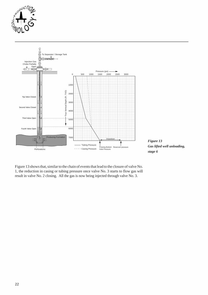
Figure 13 shows that, similar to the chain of events that lead to the closure of valve No.1, the reduction in casing or tubing pressure once valve No. 3 starts to flow gas willresult in valve No. 2 closing. All the gas is now being injected through valve No. 3.
Figure 13
Gas lifted well unloading,
stage 6

Department of Petroleum Engineering, Heriot-Watt University 23
33Gas Lift
0 500 1000 1500 2000 2500 3000
1000
2000
3000
4000
5000
6000
7000
Pressure (psi)
Tubing Pressure
Casing Pressure
True
Ver
tical
Dep
th (
Ft.
TV
D)
Producing Formation
Perforations
Top Valve Closed
Second Valve Closed
Third Valve Closed
Fourth Valve Open
Injection GasChoke Partially
Open
To Separator / Storage Tank
Reservoir pressure
Drawdown
Flowing BottomHole Pressure
The process has continued to its logical conclusion in Figure 14. Valve No. 4 has beenexposed to gas flow and valve No. 3 has shut. All the gas is being injected throughvalve No. 4 - this is the operating valve. An operating valve can be either a gas liftvalve or a simple orifice.
Figure 15 is an ideal illustration of the development of the tubing head and casing head(or gas lift) pressure with time during unloading process described in Figures 7 to 14.The sequential reduction in casing head pressure as gas is successively injectedthrough the lower gas lift valves is shown. This is not always so clearly observed inpractice. The annulus pressure is not only controlled be the settings of the gas liftvalve(s) referred to above, but also by the balance between the casing head (surface)gas injection rate and the (total) gas passage rate through the valves. Further, it canbe seen that the erratic behavior of the tubing head pressure as the well is beingunloaded is replaced by a steady value as stable production is achieved when the wellis lifted from valve No. 4.
Figure 14
The producing gas lifted
well

24
.eru
sser
Pgni
buTdnagnisaCfognidroceR
neP
niw T
DATE ON
DATE ON
TIME
TIME
AM
AM
11PMMIDNIGHT1AM
2AM
3AM
4AM
5AM
6AM
7AM
8AM
9A
M
10AM
11AMMIDDAY 1PM
2PM
3PM
4PM
5PM
6PM
7PM
8PM
9PM
10PM
1000
800
600
400
300
200
100
500
700
9001000
800
600
400300
200100
500
700
900
1000
800
600
400300
200100
500
700
900
1000800
600
400300
200 100
500
700
900
1000
800
600 40
0 300
200
100
500
700
900
1000
800
600
400
300
200
100
500
700
900
1000
800
600
400
300
200
100
500
700
900
1000
800
600
400
300
200
100
500
700
900
Open chokebleed off tubingpressure.
Liquid only beingexpelled fromtubing.
First gas to surface.
Switch ongas lift.
Stable productionvia 4th valve
Top valveuncovered
2nd valveuncovered
3rd valveuncoveredCasing head or
lift gas pressure
Tubing headpressure
4th valveuncovered
3.5.1 Safety FactorsSeveral safety factors are normally introduced when preparing gas lift designs for realwells. This is to account for:
(i) errors in the valve’s pressure settings,
(ii) errors and fluctuations in the well data, lift gas injection pressure and the estimateof the valve temperatures under flowing conditions,
(iii) the pressure drop across the valve’s choke and that required to obtain sufficientmovement of the stem.
One method by which safety factors can be built into the design is illustrated in section3.13.4
3.5.2 Gaslift Valve Spacing Criteria summarisedThe well unloading process was described in the previous section. The choseninstallation depths of valves Nos. 1 - 4 will have been based on the following criteria:
(i) Specify a minimum number of gas lift valves. This will not only reduce the costbut also the number of potential leak paths.
(ii) Gas lift valves to be installed sufficiently far apart that they do not interfere witheach other’s operation (150m suggested minimum spacing).
Figure 15
Typical casing / tubing
pressure and production
rate measurement during
unloading of a gas lifted
well.

Department of Petroleum Engineering, Heriot-Watt University 25
33Gas Lift
(iii) (continuous) Gas injection through the operating valve occurs as deep aspossible based on current producing conditions.
3.6 SIDE POCKET MANDRELS
Completion equipment is available so that gas lift valves can be permanently installedas part of the tubing. Such wells require a workover if any repairs or changes to thesettings of the gas lift system need to be made. However, most completions employside pocket mandrels (figure 16) installed at appropriate depths in the tubing string aspart of the permanent completion. Side pocket mandrels allow gas lift valves to beinstalled (and recovered) in a live well using wireline techniques. They are ovalshaped accessories with an outside diameter greater than that of the tubing {figure 16(c)}. This shape allows the gas lift valve to be installed in the pocket placed to oneside of the tubing conduit, thus maintaining fullbore access throughout the completetubing length.
Lift Gas Injection
Lift Gas InjectedVia Port in Casing Li
ft G
as In
ject
edV
ia P
ort i
n Tu
bing
Lift Gas InjectedVia Port in Casing
Pocket for GasLift Valve
Poc
ket f
or G
asLi
ft V
alve
Produced Fluidsand
Lift Gas
Gas Lift Valve
Pressure SensitiveElement (Bellows)
Seal Element
Polished Bore
Produced Fluids
Lift Gas Injection
Produced Fluidsand
Lift Gas
Produced Fluids
(a) Side pocket mandrel for injectionpressure operated valve
(b) Side pocket mandrel for tubingpressure operated valve
(c) Cross section of side pocket mandrelwith gas lift valve installed in pocket
Seal ElementFull BoreAccessThroughTubing
Gas Lift Valve Body
Polished bore
Figure 16
Schematic view of side
pocket mandrel showing
comparison of injection and
tubing pressure operated
valves
26
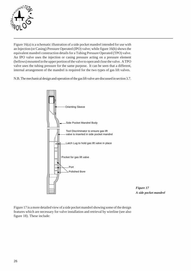
Figure 16(a) is a schematic illustration of a side pocket mandrel intended for use withan Injection (or Casing) Pressure Operated (IPO) valve; while figure 16(b) shows theequivalent mandrel construction details for a Tubing Pressure Operated (TPO) valve.An IPO valve uses the injection or casing pressure acting on a pressure element(bellows) mounted in the upper portion of the valve to open and close the valve. A TPOvalve uses the tubing pressure for the same purpose. It can be seen that a different,internal arrangement of the mandrel is required for the two types of gas lift valves.
N.B. The mechanical design and operation of the gas lift valve are discussed in section 3.7.
Orienting Sleeve
Side Pocket Mandrel Body
Tool Discriminator to ensure gas liftvalve is inserted in side pocket mandrel
Latch Lug to hold gas lift valve in place
Polished Bore
Pocket for gas lift valve
Port
Figure 17 is a more detailed view of a side pocket mandrel showing some of the designfeatures which are necessary for valve installation and retrieval by wireline (see alsofigure 18). These include:
Figure 17
A side pocket mandrel

Department of Petroleum Engineering, Heriot-Watt University 27
33Gas Lift
(a) Gas lift valve beingrun into well on wirelinetool sling.
(b) Wireline "kickover" toolplacing gas lift valve intoside pocket mandrel.
(c) Recovering wireline toolstring after latching gas liftvalve in place in side pocketmandrel.
(b) (c)(a)
(i) An orientating sleeve. This contains a device (e.g. a vertical slot) which fitsinto its counterpart (finger) on the kickover tool so that gas lift valve and knuckle ofthe kickover tool are correctly aligned with the pocket orientation. This allows thetool to insert a gas lift valve into the mandrel or to recover the gas lift valve, asappropiate.
(ii) A tool discriminator which guides the gas lift valve into the pocket whiledeflecting larger diameter tools back into the main tubing.
Figure 18
Wireline installation of a
gas lift valve in a side
pocket mandrel

28
(iii) A latch ring on the valve locks underneath the mandrel’s latch lug, securing thevalve in place. This prevents the valve becoming detached from the mandrel oncethe well is placed on production.
(iv) Fluid tight seals are created between the gas lift valve seal elements and thepocket’s polished bore. These are situated both above and below the casing port forIPO valves or the tubing port (TPO valves).
3.6.1 Other Uses of Side Pocket MandrelsThe gas lift valve Side Pocket Mandrels can also be replaced by tools with thefollowing functions:
(i) Chemical injection valves;
(ii) Differential dump/kill valves;
(iii) Circulating valves;
(iv) Circulating sleeves;
(v) Dummy valves;
(vi) Water injection control valves.
3.7 Gas Lift Valve MechanicsThe mode of action of the upper gas lift valves, in which the top valves are designedto open and close to allow the fluid in the casing/tubing annulus to be unloaded so thatdeep gas injection can be achieved, was described in the previous section. Theoperating valve is different, being designed to allow for a continuous flow of gas. Theupper gas lift valves have ports sized to pass only the required volume of gas, limitingthe rate at which the unloading takes place. A larger port is often installed in theoperating valve so that gas injection can be increased, if dictated by future well orreservoir conditions. Dummy valves are installed in the “Bracketing Envelope”where “live” valves are currently not required.
The following sections discusses the valve’s mechanical construction.
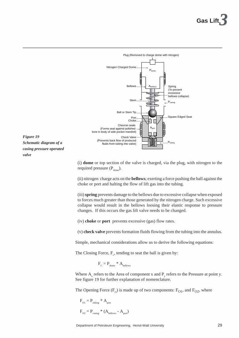
3.7.1 Casing or Inflow Pressure Operated (IPO) ValvesA schematic diagram of a casing pressure operated valve is shown in figure 19. The:
Department of Petroleum Engineering, Heriot-Watt University 29
33Gas Lift
Pdome
Abellows
Aport
Plug (Removed to charge dome with nitrogen)
Nitrogen Charged Dome
Bellows
Ptubing
Pcasing
Spring(To preventexcessivebellows collapse)
Stem
Ball or Stem Tip
Port Square Edged SeatChoke
Check Valve(Prevents back flow of produced
fluids from tubing into valve)
Chevron seals (Forms seal against polished
bore in body of side pocket mandrel)
(i) dome or top section of the valve is charged, via the plug, with nitrogen to therequired pressure (P
dome).
(ii) nitrogen charge acts on the bellows; exerting a force pushing the ball against thechoke or port and halting the flow of lift gas into the tubing.
(iii) spring prevents damage to the bellows due to excessive collapse when exposedto forces much greater than those generated by the nitrogen charge. Such excessivecollapse would result in the bellows loosing their elastic response to pressurechanges. If this occurs the gas lift valve needs to be changed.
(iv) choke or port prevents excessive (gas) flow rates.
(v) check valve prevents formation fluids flowing from the tubing into the annulus.
Simple, mechanical considerations allow us to derive the following equations:
The Closing Force, Fc, tending to seat the ball is given by:
FC = P
dome * A
bellows
Where Ax refers to the Area of component x and P
y refers to the Pressure at point y.
See figure 19 for further explanation of nomenclature.
The Opening Force (FO) is made up of two components: FO1, and FO2, where
FO1
= Ptubing
* Aport
FO2
= Pcasing
* (Abellows
- Aport
)
Figure 19
Schematic diagram of a
casing pressure operated
valve
30
and FO = F
O1 + F
O2
The Opening and Closing forces are equal just before the valve opens.
Pdome
* Abellows
= Pcasing
* (Abellows
- Aport
) + Ptubing
* Aport
or PP P (A A
(A Acasing dome tubing port bellows
port bellows
=−−
/ )
/ )1
Thus the key factors controlling the gas lift pressure required to open the valve are thedome and tubing pressures and the ratio of the bellows and port areas. IPO valvesnormally have the ratio (A
port/A
bellows) set as small as practical.
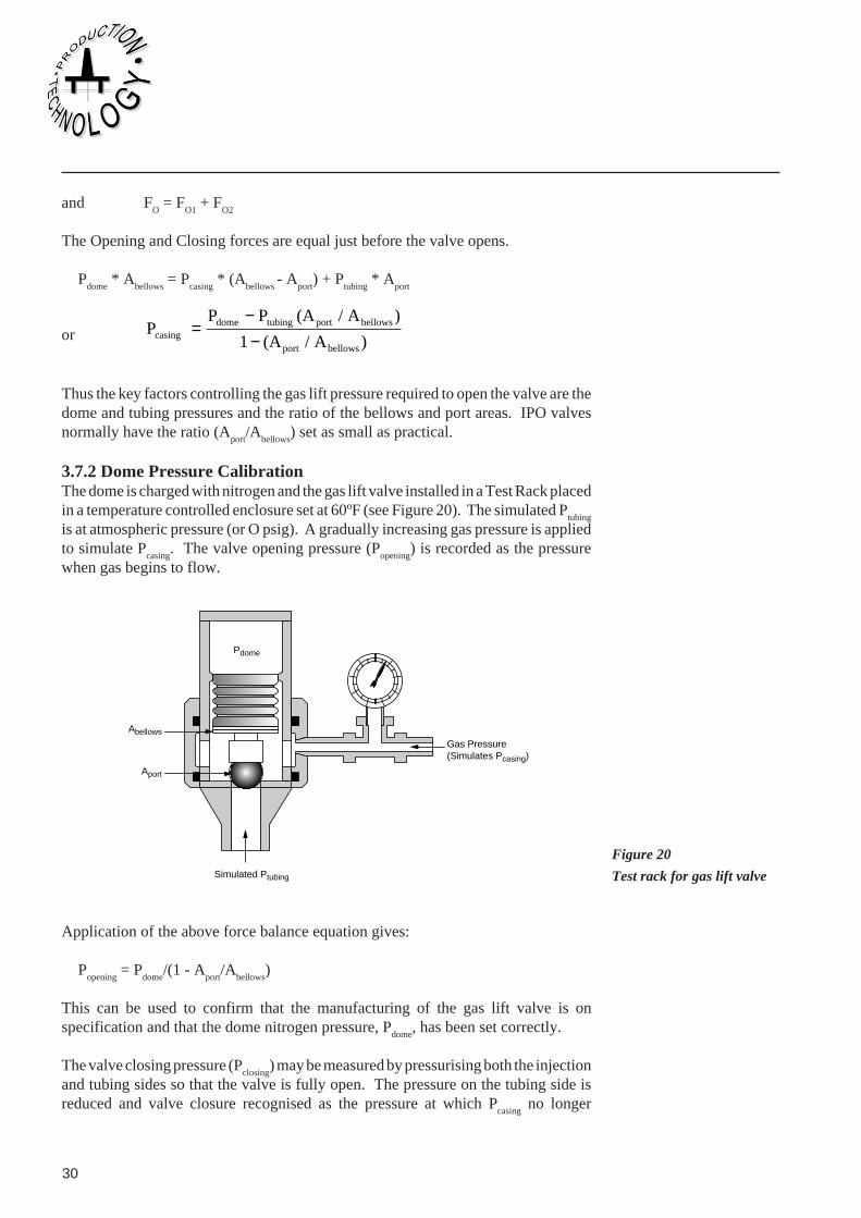
3.7.2 Dome Pressure CalibrationThe dome is charged with nitrogen and the gas lift valve installed in a Test Rack placedin a temperature controlled enclosure set at 60ºF (see Figure 20). The simulated P
tubing
is at atmospheric pressure (or O psig). A gradually increasing gas pressure is appliedto simulate P
casing. The valve opening pressure (P
opening) is recorded as the pressure
when gas begins to flow.
Gas Pressure(Simulates Pcasing)
Abellows
Aport
Simulated Ptubing
Pdome
Application of the above force balance equation gives:
Popening
= Pdome
/(1 - Aport
/Abellows
)
This can be used to confirm that the manufacturing of the gas lift valve is onspecification and that the dome nitrogen pressure, P
dome, has been set correctly.
The valve closing pressure (Pclosing
) may be measured by pressurising both the injectionand tubing sides so that the valve is fully open. The pressure on the tubing side isreduced and valve closure recognised as the pressure at which P
casing no longer
Figure 20
Test rack for gas lift valve

Department of Petroleum Engineering, Heriot-Watt University 31
33Gas Lift
decreases in line with Ptubing
. The design of the valve dictates that Pclosing
will be lowerthan P
opening, since starting from the open valve situation means that the injection
pressure acts on the complete bellows area.
The valve spread is defined as the difference between the valve test rack opening andclosing pressures i.e. (P
opening - P
closing). It is a measure of the difference between the
effective area of the bellows and the port. Figure 21 illustrates a typical valve spreadand its variation with changes in the casing pressure.
Pressure (psi)
Throttling flow region
Gas
inje
ctio
n ra
te (
MM
scf/d
)
Critical flow through a square edged orifice (same diameter as choke installed in gas lift valve)
Sub - criticalflow regionGas lift valve performance with
casing pressures (b), (c), (e) and (d)
Pcasing
P casing (b)
P casing (d)P casing (c)
Valve spread at various values of Pcasing
(e)
(a)(d)(c)(b)
3.7.2.1 Temperature CorrectionA compressible fluid (gas) is required for charging the dome (to avoid valve ruptureas the fluid heats up when it is run into the well or the well heats up when it is placedon production). Nitrogen is used for this purpose since it is non-corrosive, inflammableand the temperature effect on the pressure is well known.
P2 = P
1 * T
c
and TcTT
= + −+ −
{ . * ( )}{ . * ( )}1 0 00215 601 0 00215 60
2
1
where P1 = gas Pressure at Temperature T
1 (oR),
P2 = gas Pressure at Temperature T
2 (oR),
Tc = Temperature Correction factor
In practice, part of the dome volume is filled with a silicone liquid to dampenvibrations created by the gas flow through the valve. This silicone liquid occupies partof the volume of the dome, reducing the effective volume of the nitrogen charge.However, it will also expand as the valve heats up, giving an additional pressureincrease to that calculated above. This secondary correction becomes less importantfor the larger (1.5") valves where the volume of liquid compared to the gas volume isrelatively less important.
Figure 21
Valve performance
32
3.7.3 Valve Flow Performance
The operating valve at the bottom of the gas lift string, through which gas will becontinually passed, is normally equipped with square edged, orifice choke. Theresulting flow performance is shown in figure 21, curve (a). The gas flow rate passingthrough the choke increases with increasing pressure difference between the casingand tubing until a maximum value is reached when the critical flow rate is achieved.At this point the gas flow velocity has become supersonic and the volume of gas passeddoes not increase further with increasing pressure differential. The valve is oftenreferred to as being “choked” at this point. Orifice flow is described by the “Thornhill-Craver equation” which relates flow capacity to the difference between injection gasand tubing pressure at the valve depth and the port (orifice) size (see chapter 3.13). Theorifice size determines the maximum or “choked” volume of gas that can be injectedto aid lifting the well fluids to the surface.
This equation is often (incorrectly) used to describe the gas flow through an IPO orTPO gas lift valve. The Thornhill-Craver equation assumes that the flow through thevalve’s port is unimpeded by the presence of the ball, i.e. it assumes the valve is fullyopen and the ball does not impede the passage of gas. (Dynamic) Valve Response tests(see below) have shown that the Thornhill-Craver equation can overpredict the actualflow rate by more than 200%.
Further, simple gas lift design procedures assume that the valve will shut immediatelythe casing (IPO valve) or tubing (TPO valve) pressure drops below the preset value.This “instantaneous-closure” assumption is not correct, creating an even greater errorwhen Proportional Response Valves (see section 3.7.4) are used.
3.7.3.1 Dynamic Valve PerformanceDynamic testing of the valve, in which the injection gas flow rate is measured for afixed casing pressure and a range of tubing pressures, is required to properlyunderstand the valve’s performance. These dynamic valve performance characteristicsdescribe the:
(i) valve’s ability to start passing gas when the ball first lifts from its seat,
(ii) rate of increase in the gas flow rate as this clearance increases (flow capacity),
(iii) corresponding decrease in gas flow rate as the valve closes and
(iv) resistance to vibration under flowing conditions.
The valve's load rate (measured in units of psi/inch) is the pressure differencerequired to move the stem a given distance; while the valve spread is the differencebetween the opening and closing pressures. The shape of the performance curverepresents the valve’s sensitivity to pressure.
The American Petroleum Institute has published a Recommended Practice (NumberIIV2 or API RP IIV2) which describes a standardised testing procedure to measure aparticular gas lift valves dynamic performance. The standard is summarised as follows:

Department of Petroleum Engineering, Heriot-Watt University 33
33Gas Lift
The valve is installed in the test equipment after being set up with a suitable domepressure using the manufacturer’s recommended procedure. Measurements are madeof the:
(i) valve opening pressure,
(ii) pressure increase required to move the stem to its value of maximum travel and
(iii) position of the stem for various intermediate pressures.
The maximum effective travel distance influences the volume of gas that the valve canpass. The maximum effective stem travel (test one) needs to be measured only oncefor each valve design.
The flow capacity of the valve (as a function of stem position) is tested in a separatetest designed to measure the valve’s flow coefficient (or C
v). In this test the stem is
adjusted to various positions between 5% and 100% of its maximum value and theflow rate measured at 5 differential pressures - one of which should display chokingflow (see above). This flow coefficient test and the dynamic test (see below) need tobe carried out for each size of choke (or port) that are planned for installation in thevalve.
Pressure (psi)
Throttling flow region
Gas
inje
ctio
n ra
te (
MM
scf/d
)
Critical flow through a square edged orifice (same diameter as choke installed in gas lift valve)
Sub - criticalflow regionGas lift valve performance with
casing pressures (b), (c), (e) and (d)
Pcasing
P casing (b)
P casing (d)P casing (c)
Valve spread at various values of Pcasing
(e)
(a)(d)(c)(b)
A final test is performed for several set pressures in which the injection (or tubing)pressure is slowly decreased (or increased). The flow rate is measured at a numberof pressures until the valve closes. Either procedure should give the same result. Theresults of such a testing scheme is illustrated in figure 21. Here, the valve’s flow ratehas been measured at four casing pressures {P
casing (b), (c), (d) and (e)} and a variety of tubing
pressures. N.B. A fixed port size and dome pressure was used for all these tests.
Curve (b) shows the performance with the casing pressure adjusted to Pcasing(b)
. The gasflow rate is initially zero, even though the valve is open, since the tubing pressure isset to the same value. Gas starts to flow into the tubing when the tubing pressure isreduced, though the flow rate will not increases so rapidly as recorded for curve (a)- the equivalent test with a square edged orifice.
Figure 21
Valve performance

34
N.B. Pcasing(a)
and Pcasing(b)
have the same numerical value in figurer 21. It can be seenthat the gas flow rate passed by the valve {curve(b)} initially increases at a slightlylower rate than that for the orifice {curve (a)} of the same diameter as the gas liftvalve’s port. This difference is due to the ball, positioned slightly downstream of thevalve’s port (see figure 19), interfering with the gas flow pattern through the valve.
Further reductions in tubing pressure will increase the gas flow rate until a maximumis reached. After this point, the valve’s closing force (F
C) becomes relatively greater
than the opening force (FO); allowing the ball to move closer to its seat and reduce the
gas flow. This gas flow reduction occurs in a (relatively) linear manner (the “throttlingregion”) until it has decreased to zero at P
tubing(b). The slope of the gas flow rate / tubing
pressure plot in the throttling region is a function of the gas lift valve’s mechanicaldesign.
The dynamic valve performance at a slightly lower casing pressure {Pcasing(c)
} has asimilar shape (determined by the gas lift valve’s mechanical design). The maximumgas flow rate and the corresponding valve “spread” are now smaller since the valveopening force (F
O) has been reduced by the lower value of the casing pressure.
This process continues further when the casing pressure is reduced to Pcasing(d)
. Hereonly a small gas flow rate is recorded over a small range of tubing pressures. Oncethe casing pressure is set equal to, or lower than, P
casing(e), the valve will no longer open
and gas can not flow into the tubing.
N.B. It will be discussed later (3.13.4) that each gas lift valves in a completion stringshould be set up with an opening pressure slightly lower (typically 50 psi) than thesetting of the valve above it. This progressive lowering of the setting pressure for thedeeper valves aids the closure of the upper valves so that the gas injection isprogressively transferred to lower valves during the unloading process. It should benoted here that IPO valves do not control the annulus pressure. A drop in the annularpressure can only occur when the gas injection rate, possibly through both valves, isgreater than gas flow rate into the casing annulus at the surface.
3.7.3.2 Valve Performance Flow ModelSophisticated, computerised gas lift design programs require quantitative modelswhich describe the above flow tests. The Thornhill-Craver model {figure 21, curvea}, the previous industry standard, describes the flow through orifices reasonable wellbut does not capture the throttling action of “real” gas lift valves. (The originalpublication proposed the equation to describe flow through surface chokes with fixedbeans!) An extension of this model, by Winkler and Eads, uses the same formulae butsubstitutes the actual choke or port area open to flow rather than the fully open valveused by Thornhill-Craver. Despite using a constant discharge coefficient for all stempositions, the flow curves generated by the Winkler-Eads model have the correctshape {figure 21(b) et seq.}. It works well (accuracy 20-30% over the full pressurerange) for valves with a port size of less than 0.25", though the errors rise to >100%when ports >0.25" are installed.
Both the Thornhill-Craver and the Winkler-Eads equations have an idealised, mecha-nistic basis - the equqtions are not “tuned” using the actual flow test data measured in

Department of Petroleum Engineering, Heriot-Watt University 35
33Gas Lift
the API test procedure described above. These gas flow rate measurements can berepresented by:
(i) a Flow Coefficient (Cv). This is a measure of the gas flow rate as a function of
pressure differential across the valve
(ii) the distance of the stem from its seat.
The Flow Coefficient (Cv) also determines the pressure rates at which choke flow
occurs across the valve as a function of the stem position. This is an important factorsince most valves show choke flow when the gas injection is being transferred to thenext lower valve. A higher value of C
v implies a greater valve flow capacity. It’s value
is determined by the:
(i) valve inlet port location with respect to the seat,
(ii) actual profile of the seat or valve,
(iii) design of the cross over ports and
(iv) any flow restrictions downstream of the port e.g. the check valve.
The measured Cv values are useable over a wide range of temperature and pressure
conditions, as well as for both liquid and gas flow. They can be used for all valves ofthe same type and port size. However, any design change which alters the flow paththrough the valve will effect the value of C
v and require that the flow test be repeated.
API RP IIV2 recommends a simplified approach to analysing this flow data using Cvvalues. Alternative approaches have been proposed by:
(i) Tulsa University Artificial Lift Project (TUALP) using a statistical approach todata analysis. This can only be applied over the pressure range used for the flow tests.
(ii) Valve Performance Cleaning-house (VPC). The VPC method uses a mechanisticmodel based on the force balance equation and load rate to calculate a value of C
v;
which is then adjusted so as to be able to reproduce the dynamic test data.

36
3.7.4 Proportional Response ValvesThe design of a Proportional Response Valve (see figure 22) involves:
Pdome
Abellows
Aport
Plug (Removed to charge dome with nitrogen)
Nitrogen Charged Dome
Bellows
Ptubing
PcasingStem
"Stop" to prevent excessivebellow collapse
Large Ball
PortTaperedSeatChoke
Check Valve(prevents back flow of produced
fluids from tubing into valve)
Chevron seals(form seal against polished borein body of side pocket mandrel)
Spring(To provideproportionalresponse)
(i) The addition of a spring to counterbalance the force trying to expand the bellows,
(ii) A “stop” to prevent excessive bellows collapse,
(iii) A larger ball at the tip of the stem and
(iv) A tapered seat instead of a square edged seat.
The proportional response valve has more parts than the “traditional” valve. It usesmore “O” rings, which are not only expensive but also prone to failure i.e. ProportionalResponse Valves should only be specified when definite operational advantages havebeen identified.
3.7.5 Dynamic Valve Response and Gas Lift Completion ModelingSimple (manual) gas lift completion design programs assume that the valves will openfully at (casing or tubing) pressures slightly greater than the set value and willcompletely close when the pressure drops below this value. They assume that the well“jumps” immediately from steady state operation when lifting through one (fullyopen) valve to a second, steady state condition when lifting through the next deepervalve. In practice:
(i) the volume of gas injected through a given valve will vary with time.
(ii) the well will only reach steady state inflow a considerable period of time afterthe unloading process has finished.
Figure 22
Proportional response gas
lift valve

Department of Petroleum Engineering, Heriot-Watt University 37
33Gas Lift
(iii) the combination of changes in (i) and (ii) will result in continuous changes inthe well’s Gas Liquid Ratio (GLR) during the unloading process. This is especiallytrue when any fluid lost to the formation during the workover or the early stages ofwell unloading has to be produced first before live formation fluids can enter the welland improve the well outfllow.
(iv) there is a significant volume of gas in the casing/tubing annulus. Pressurechanges will not occur instantaneously due to the limited gas supply rate at thesurface or the finite gas flow rate through a particular valve.
(v) the valves can open and close a number of times during the unloading of a multi-valve completion string e.g. as well temperature changes.
(vi) the temperature changes during the unloading process (being neither thegeothermal nor the steady state flowing temperature gradient).
It can be appreciated that a transient rather than a steady state computer program isrequired to simulate the unloading process. Such programs must accurately predictthe development of the above parameters as a function of time. The output of theprogram will include, as a function of time, the:
(i) tubing and annulus pressure at valve depths as well as surface casing (annulus)and tubing head pressure,
(ii) flow rate of liquid and gas through open valves,
(iii) depth of liquid levels in tubing and annulus,
(iv) volume of fluids (gas and liquid) produced to the surface and
(v) inflow from the reservoir (after making allowance for any liquid lost to theformation, as discussed above).
One commercially available program is DynaliftTM marketed by Edinburgh PetroleumSystems. It has been shown to be useful for troubleshooting problematic wells e.g. theprediction of when the following difficulties can be expected during well unloading- erosion of (gas lift) valves, severe slugging, excessive well stabilisation times etc.
3.7.6 Well StabilityDynamic Well Simulation programs can also be used to evaluate potential causes oflift problems once the well has been placed on production. These valve problemsmanifest themselves by the:
(i) well not producing or producing at lower than expected rate,
(ii) unstable well behaviour (casing and/or tubing head pressures oscillate regularly)and
(iii) excessive unloading and well stabilisation times.

38
The quickest method to correct the problem is to identify which valve is the cause ofthe production difficulty and then replace it with a correctly calibrated replacement.The alternative, to replace the gas-lift valves in a random, ad hoc manner is often muchmore time consuming and may never solve the problem.
Comparison of the actual and the predicted well behavior allows identification of thetype of problem being experienced as well as which gas lift valves is the cause of theimproper operation. Typical problems which have to be diagnosed include:
(i) valves that have become either:
(a) (partially) plugged or
(b) enlarged (cut out)
(ii) valves set to:
(a) incorrect dome pressures or
(b) operating incorrectly due to mechanical problems and
(iii) multi-pointing (injection through more than one valve at the same time). Thisis often due to an upper valve opening and closing.
An example of a specific operational problem that could be diagnosed is the case whenthe surface gas injection rate is greater than the single valve flow rate calculated fromthe annular and tubing pressures. Possible causes include:
(a) gas injection through two or more valves,
(b) the valve choke (or port) of the operating valve was enlarged (cut out) duringunloading or
(c) an upper valve is opening and closing.
A quantitative evaluation of the flow rates and the tubing and casing pressure valuesand their stability are required to differentiate between the above causes, as well as toidentify the specific problem valve.
3.8 GAS LIFT DESIGN PROCEDURES
This chapter will discuss the procedure used to design the gas lifted well. It willcombine the flow performance of operating valves discussed above with the conceptsdiscussed in Section 1 on multiphase flow and Nodal Analysis. Table 4 lists the welldata required to initiate this design process which will enable us to specify theoptimum:

Department of Petroleum Engineering, Heriot-Watt University 39
33Gas Lift
Tubing Outside Diameter 4.5 in
Tubing weight 12.6 lb/ft
Deviation Survey Vertical Well
Target Production Rate 5000 bfpd
Watercut 60% vol.
Produced Water Density 1.06 g/cm3
Gas Relative Density 0.65
Packer Setting Depth 9,500ft.
Mid Perforation Depth 10,000ft.
Wellhead Flowing Pressure 100 psig
Shut In Bottom Hole Pressure 3,700 psig
Productivity Index 0.50 STB/d/psi
Oil Gravity 37 API
Bubble Point 1200 psig
Gas Oil Ratio 400
Gas Injection (Casing) Pressure 1500 psig
Gas Available For Injection 3 MM scf/d
Ambient Temperature at Surface 70 F
Flowing Temperature at Surface 140 F
Temperature at Mid Perforation 240 F
Kill Fluid Gradient 0.45 psi/ft. *
* In Annulus / Tubing for Unloading Calculations
(i) Tubing size,
(ii) Injection gas supply parameters (pressure and volume),
(iii) Installation depth of operating valve and
(iv) Separator pressure.
The first item is to check that gas lift valves can be placed at suitable distances abovethe operating valve to ensure that the well can be unloaded using the gas lift parameterschosen (see section 3.5). The gas lift design will have to be changed if it is found thatthe well cannot be unloaded. Further, the design will be influenced by the gas liftdesign philosophy. For example:
(i) A Maximum Production / Expected Case Design would:
(a) maximise production by injecting gas as deep as possible,
(b) install extra gas lift valves around the operating valve to allow the depthof the operating valve to be adjusted and
(c) budget for (some) well entries to be required since the well may stopproducing if well inflow conditions change.
(ii) Worst Case / Robust Design would be designed to:
Table 4
Data set for gas lift design

40
(a) always work by placing the operating valve at a relatively shallow depthcompared to that normally achieved with to the available gas lift pressure.
(b) results in a lower production rate. Deferred production probably alsoimplies a reduced reserve recovery.
The philosophy chosen for a particular well / field will depend on the operationalconditions and the cost scenario.
3.8.1An Example Design - optimising the performance of a gas lifted wellThe first requirement is to study the well’s in- and out-flow and confirm that artificiallift is required. This is illustrated in figure 23. It can be seen that the well productionrate will decrease rapidly once well Edinburgh-1 begins to produce water. It will stopflowing when the water cut reaches 30%. Any reduction in the flowing sand facepressure due to depletion of the reservoir pressure and / or the development of a nearwellbore “skin” due to Formation Damage (see Chapter 4 of Production TechnologyII) will reduce the well production rate. This will also reduce the critical water cut atwhich natural flow ceases. It should be remembered that the form of the InflowPerformance Relationship used to describe fluid inflow from the formation (e.g.Vogel or “straight line PI”) will have an impact on these calculations.
Well production rate
San
dfac
e flo
win
g pr
essu
re
Reservoir inflow at various water cuts
60%40%20%
80%
0%
Tubing outflow at various water cuts 80%
0%
We will assume that Gas Lift has already been identified as the most suitable form ofartificial lift for this well and an operating valve has been installed at a suitable depth.The impact of the injection of varying amounts of gas on the well production rate isevaluated in Figure 24. Figure 25, a plot of production performance against lift gasinjection rate can now be derived. It can be seen that the injection of the first 1.25MMscf/d of lift gas leads to a rapid increase in production rate. Further increases inthe rate of gas injection yields ever reducing benefits until a maximum production rateis reached at 2.5 MMscf/d. The same data are plotted in Figure 26. Here the lift gasinjection rate is represented as a Gas-Liquid Ratio - the sum of the Produced fluid gasliquid ratio and the gas injection rate divided by the (gross) liquid production rate. Asexpected, the graph shows a maximum production at the 2.5 MMscf/d gas injection rate.
Figure 23
Performance well
Edinburgh - 1 at varying
water cuts

Department of Petroleum Engineering, Heriot-Watt University 41
33Gas Lift
Well production rate
Sandfa
ce flo
win
g p
ress
ure
Natural flow
ReservoirInflow
All at40%Watercut
j
0.5
1.25
3.75
2.5
Lift gas injection rate (MM scf/d)
Lift gas injection rate (MMscf/d)
Well
pro
duct
ion r
ate
0 1.25 2.5 3.75
3.75 MM scf/d
2.5 MM scf/d
1.25 MM scf/d
0.5 MMM scf/d Maximum production rate
Well production rate
Gas
- L
iqui
d R
atio
g q
(Technical) Optimum gasinjection rate
Formation Damage - or the presence of a near wellbore skin - will reduce the wellproductivity. Figure 27 is similar to Figure 24, except that the reservoir inflow froma damaged well (skin = +6) has also been plotted. Figure 28 not only illustrates thisloss in well productivity due to the presence of the skin, but also indicate that theconclusion drawn as to the optimum gas injection rate is unchanged.
Figure 24
Sensitivity study for tubing
outflow to lift gas injection
rate at 40% water cut
Figure 25
Production performance
and gas lift injection rate
Figure 26
Production performance
against gas liquid ratio

42
Well production rate
San
dfac
e flo
win
g pr
essu
re
Natural flow
ReservoirInflowskin = 0
40%Watercut
j
0.5
1.25
3.75
2.5
Reservoirinflowskin = +6
x
x
x
x
x
x
Lift gas injection rate (MM scf/d)
Lift gas injection rate (MMscf/d)
Wel
l pro
duct
ion
rate
0 1.25 2.5 3.75
Skin = 0
Skin = +6
Figure 29 examines the effect of changing the depth of lift gas injection. A deepinjection point creates a greater drawdown leading to an increased production rate anda more efficient GUF (Gas Utilisation Factor or Gross production rate / Gas InjectionRate).
Lift gas injection rate (MMscf/d)
Wel
l pro
duct
ion
rate
0 1.25 2.5 3.75
Incr
easi
ng d
epth
of i
njec
tion
Figures 30 and 31 examine the sensitivity of the well production rate to an increase inthe diameter of the production tubing. The production increases rapidly as the tubingOD increases to 4.5 in, but then decreases for the largest tubing (5.5 in). Excessiveslip between the gas and liquid phases occurs at the lower flow velocity associatedwith the larger tubing.
Figure 28
Production performance
and lift gas injection rate
for an impaired well
Figure 29
Production performance
and lift gas injection depth
Figure 27
Sensitivity study for tubing
outflow to lift gas injection
rate at 40% water cut for
an impaired well

Department of Petroleum Engineering, Heriot-Watt University 43
33Gas Lift
San
dfac
e flo
win
gpre
ssur
e
Well production rate
2.875" Tubing OD
Well inflow at40% Water cut
3.5"4.5"
5.5"
Wel
l pro
duct
ion
rate
Tubing internal diameter (in)2 2.5 3 3.5 4 4.5 5
3.5"OD
4.5"OD 5.5"OD
2.875"OD
2 2.5 3 3.5 4 4.5 52 2.5 3 3.5 4 4.5 5
We showed in Chapter 1 (Well Performance) that separator pressure affected theoutflow performance of naturally flowing wells. The same is true for gas lifted wells- Figure 32 show how the well outflow performance improves as the separatorpressure is decreased. This is shown explicitly in Figure 33, where the production rateis plotted as a function of separator pressure. In general, the lower the separatorpressure, the higher the production rate.
San
dfac
e flo
win
g pr
essu
re
Well production rate
Separator pressure (psi)
Well inflow at40% Water cut
250200150100
5025
75
Figure 30
Sensitivity study of tubing
outflow at various to tubing
diameters
Figure 31
Production performance
and tubing diameter
Figure 32
Sensitivity study of tubing
outflow to separator
pressure

44
Wel
l pro
duct
ion
rate
Separator pressure (psi)0 50 100 150 200 250
It should be emphasised that, in addition to the separator pressure, a back pressure onthe well performance is created by pressure losses across:
(i) Valves (should be fully opening type to minimise any pressure losses)
(ii) Choke body and/or choke nipples, if installed
(iii) The flowline (particularly pipe elbows) and long narrow diameter, tortuousflow lines with the separator mounted at a higher elevation than the wellheadcause an increased back pressure.
(iv) The wellhead itself (a Y block design will have a reduced pressure losscompared to the standard T block for a high rate well)
A further parameter that needs to be optimised is the lift gas injection pressure - Figure34 illustrates the effect this has on the well outflow performance while Figure 35records the production rate with changes in injection gas pressure.
Sandfa
ce flo
win
g p
ress
ure
Well production rate
Well inflow at
40% Water cut
Gas injection lift pressure
400
600
800
1000
12001500
Figure 34
Sensitivity study of tubing
outflow curves to gas
injection pressure
Figure 33
Production performance
and separator pressure

Department of Petroleum Engineering, Heriot-Watt University 45
33Gas Lift
W
ell
pro
duct
ion r
ate
Gas injection pressure (psi)500 750 1000 1250 1500
N.B. This well is capable of production with low injection gas pressures because thedepth of the operating valve was not too deep and the well was almost capable ofproducing under natural flow.
The conclusions reached from the above sensitivity studies are valid for the Edinburgh-1 well producing under the chosen combination of Reservoir Pressure and waterproduction studied. The conclusions need to be tested for robustness by repeating thesensitivity analysis for combinations of water cut and reservoir pressures that areexpected to be encountered during the well’s lifetime. Planned recompletions e.g.extension of the perforated interval, should also be included in this. Figure 36 is atypical example of the deterioration of the Reservoir Inflow Performance at varioustimes (T
1, T
2 and T
3) under the twin influences of the decrease of reservoir pressure
and increasing water cut. The tubing (outflow) performance is plotted for theoptimum gas injection rate that maximises the well production for each reservoirinflow curve i.e. the optimum gas injection rate changes with time. The GUF willdecrease with time due to the:
Well production rate
San
dfac
e flo
win
g pr
essu
re
T1
T3
T2 Reservoirdepletion Gas injection rate adjusted
for each reservoir inflow curvein order to maximise production
Reservoir inflow
x
x
x
(i) Increasing average liquid density (increasing water cut).
(ii) Decreasing (own) gas production rate (decreasing net oil production and somereservoir drive mechanisms e.g. solution gas) and
(iii) Reducing reservoir pressure.
Figure 35
Production performance
and gas injection pressure
Figure 36
Performance of well
Edinburgh - 1 at various
times

46
Figure 37 records the decreasing well production resulting from the changing wellinflow and tubing outflow performance curves, being derived from the data presentedin Figure 36.
Wel
l pro
duct
ion
rate
TimeT1 T2 T3
x
x
x
One further variable to be discussed is the choice of the multiphase flow correlationused to calculate the well outflow performance. This can have a great influence on theresults, as discussed in Chapter 1 (Well Performance). The flow correlation can bechosen on the:
(i) basis of production experience in other, similar wells in the same field,
(ii) theoretical considerations based on a comparison of the well type with theparameters originally used to generate the correlation or
(iii) c omparison of predicted and actual well performance.
The latter is the best choice when (field) data is available. The actual and predictedgas lifted well performance need to be compared at a range of gas lift injection rates.{Chapter 1 discussed how the flow correlation for a naturally flowing well could bechosen by comparing the predicted and the measured pressure traverse (the pressure-depth profile).} Figure 38 illustrates how the use of an inappropriate correlation canlead to false expectations as far as the well production rate is concerned. Flowcorrelation number 4 refers to “Hagedorn and Brown”, probably the one mostfrequently used to describe the performance of gas lifted wells. The preferred flowcorrelation for the gas lifted well may be different from that previously used todescribe the same well’s performance under natural flow.
Figure 37
Performance of well
Edinburgh - 1 as the
reservoir pressure depletes

Department of Petroleum Engineering, Heriot-Watt University 47
33Gas Lift
Lift gas injection rate (MM scf/d)W
ell p
rodu
ctio
n ra
te
Actual well data
1
23
4,5
6
0 1.5 3 4.5
Flow correlation
Tubing Size 4.5"(O.D)
Separator Pressure As low As Possibleφ
Gas Injection Pressure 1000 or 1200 psi*
Gas Injection Rate 1MM scf/d
Flow Correlation Hagedorn and Brown
* Depends on detailed cost calculationsφ Some operators have profitably reduced back pressure on the
well by "twinning" the flow line to the separator
Table 5 summarises the conclusions from the above gas lift design exercise. Chapter10 of this module discusses the need to develop a well / field model to model currentand predict future production performance as well as to systematically monitor anydifferences between this prediction and the actual measured values. Such a monitoringprocess will gather the basic data needed to test whether the chosen inflow and outflowcorrelations are still appropriate. For example, table 6 illustrates the correlations usedby one operator to achieve the most accurate predictions based on such a monitoringprogramme.
Inflow < 50% Water Cut Vogel
>50% Water Cut "Straight Line" PI
Outflow < 10,000 bfpd Hagedorn and Brown
> 10,000 bfpd Duns and Ross
3.8.2 An Example Design - Gas Lift Unloading CalculationsThe section above describes how the operating valve location and the designobjectives for the gas lift system can be chosen. An illustrative description of theUnloading Process was given in section 3.5 and Figures 7 to 15. Concerns, to beavoided by careful design of the unloading process to be followed in a particular wellare that the:
(i) Well does not unload resulting in the gas being injected at a shallow depth. Thiscan be overcome by employing a conservative design philosophy to valve spacing.
(ii) Well does not lift at an optimal rate since the above conservative designphilosophy has resulted in the operating valve being situated at too shallow a depth.
Figure 38
Sensitivity of production
performance under gas
injection to choice of
multiphase flow correlation
Table 5
Summary of chosen gas lift
parameters
Table 6
Preferred correlations

48
This can be overcome by carrying out the gas lift design using the expected wellproperties. However, if an incorrect choice of well conditions are made, this mayresult in the well being unable to unload).
(iii) The well is stymied i.e. there is a combination of conditions under which all thegas lift valves close and no more gas can be injected.
These two approaches are compared in the worked example summarised in section 3.13.
3.8.3 Further Gas Lift System ConsiderationsTwo further points need to be evaluated.
(i) Flow Velocity. Corrosion / erosion of the tubing can become excessive if acritical flow velocity. Exceeding this limit will lead to excessive maintenance costse.g. early replacement of damaged tubing or accessories. This is particularly true ifsignificant quantities of formation solids e.g. sand are being co-produced with theformation fluids. One operator sets a maximum velocity of 12 ft/s in 3.5 in tubingfor these conditions. The American Petroleum Institute published recommendationsin this area tend to be somewhat conservative, one needs to compare them with localexperience. The critical value for the onset of corrosion / erosion can be verysensitive to the composition of the produced fluid; in particular the concentrationsof carbon dioxide and hydrogen sulphide in the gas phase.
(ii) Shear Rates. Exposing water and oil mixtures to high shear rates can lead tothe formation of emulsions. The produced fluid experiences increased velocitieswhen gas lift is introduced. This is due to the improved production rate and theincreased gas oil ratio. The increased shear rates can result in the formation ofviscous emulsions, especially when a choke or bean is included in the surface flowlines, though it is difficult to predict the precise conditions which will lead toemulsion formation. The well model will need to be adapted to the field data by“tuning” the fluid properties if emulsion formation is observed.
3.8.4 Further Gas Lift System Calculations
(i) Annulus Gas Pressure with Depth
The maximum depth at which gas can be injected into the tubing is controlled by thesurface (casing) gas pressure, the pressure drop across the gas lift valve and the tubingpressure gradient. Most lift gas systems operate at between 1000 and 1200 psi and arefilled with a natural gas with a high methane content. A useful “rule of thumb” is thatthe gas pressure gradient can be approximated to 30 psi/1000 ft. A more exact valuecan be calculated from the equation:
P PRD * L
TL Sgas
av
=
exp. * *53 34 Z
where: PL
= gas pressure at depth L (psia)P
S= surface gas pressure (psia)
L = true vertical depth (ft)

Department of Petroleum Engineering, Heriot-Watt University 49
33Gas Lift
RDgas
= gas relative density (to air)T
av= average temperature of gas column (°R)
Z = gas compressibility factor at Tav and P
av
Pav
= {PS + P
L}/2
(ii) Stored Gas Volume
A considerable volume of gas is stored in the casing/tubing annulus. It can beestimated from the gas equation:
V VP T
P Tannulusav
av
=
**
* *Z
where V = the gas volume at standard conditions (ft3)V
annulus= total annular volume (ft3)
Pav
= average gas pressure in annulus (psia)P = pressure at standard condition (14.3 psia)T = temperature at standard condition (460 °R)T
av= average temperature in annulus (°R)
and Vannulus
= 0.022 * L * {dic
2 - det
2}
where L = (along hole) length between well head and tubing packer (ft)d
ic= internal casing diameter (in)
det
= external tubing diameter (in)
(iii) Gas Compressor Power Requirements
The power required by the gas compressor which will supply gas to the lift system canbe estimated from
HHP 2.23*10 * QPP
4 out
in
=
−
−
0 2
1.
Where HHP = power required (hydraulic horse power)Q = gas injection rate (scf/d)P
out= compressor outlet pressure (psia)
Pin
= compressor inlet pressure (psia)
3.9 OPERATIONAL PROBLEMS
Typical problems associated with the operation of gas lifted wells include:
3.9.1 Gas QualityThis can lead to:

50
(i) Blockage of gas injection lines due to (solid) hydrate formation during periods oflow ambient temperatures. Such blockages are most easily removed by depressuris-ing the line since hydrates are unstable at low pressures, decomposing into theirconstituent components of gas and water. The problem can be avoided by properdrying of the gas so that water dew point is below the lowest expected ambienttemperature (see Chapter 8, Oil and Gas Processing).
(ii) Loss of casing integrity due to use of corrosive lift gas. This is associated withthe presence of the acid gases (carbon dioxide and hydrogen sulphide) in the naturalgas. Guidelines are available to determine at which concentrations corrosion can beexpected. Often part of the produced gas will be sold, only sufficient gas beingretained in the lift gas system to “top-up” losses. In this case, all the gas is normallytreated to sales gas specification. Such specifications will typically limit the carbondioxide concentration to 2 or 3%, while hydrogen sulphide levels above 4 ppm areunacceptable.
In the case that none of the produced gas is sold, it may be practical to tolerate higherlevels of these acid gases. The resulting problems, from these more relaxed, gasquality specifications which will need to be resolved include:
(i) Natural gas containing carbon dioxide is only corrosive in the presence of liquidwater rather than gaseous water. Corrosion should be looked for in those pointswhere liquid water can collect (the bottom of pipelines, low points in undulatingpipelines etc.) when the partial carbon dioxide pressure exceeds 30 psi.N.B. The partial pressure of a gas corresponds to its concentration (expressed as amolar fraction) multiplied by the total system pressure.
Higher carbon dioxide partial pressures require either the specification of specialmetallurgy e.g. 13 chrome stainless steel, tubing or the continuous injection of acorrosion inhibitor. This corrosion inhibitor will passivate metal surfaces byforming a protective layer. High gas flow velocities (typically above 30-50 ft/s) willstrip the inhibitor from the metal surfaces and remove this protection.
(ii) Hydrogen sulphide partial pressures of greater than 0.05 psia lead to sulphidestress cracking of many of the steels used in completion systems and pipelines (inparticular, those with a Rockwell C hardness of greater than 22). A partial pressureof 0.05 psia hydrogen sulphide corresponds to approximately 50 ppm hydrogensulphide in a system operating at 1000 psi. Higher hydrogen sulphide levels can becoped with by specifying the appropriate metallurgy. Injection of corrosioninhibitors to passivate metal surfaces is possible on a temporary basis to protectagainst excess hydrogen sulphide levels. It is not normally recommended on apermanent basis since the sulphide stress cracking proceeds rapidly if inhibitoraddition is accidentally halted.
3.9.2 Solids These may either be produced from the formation {e.g. sand - see Chapter 7 (SandControl) or formed from the produced fluids {inorganic and organic scales - seeChapter 4 (Formation Damage)}. Wax is the most frequently encountered solid in gaslift operations}. Whatever the cause, the presence of solids within the production

Department of Petroleum Engineering, Heriot-Watt University 51
33Gas Lift
tubing can be expected to result in operational difficulties when carrying out wirelineoperations such as changing gas lift valves.
Excessive sand production can only be prevented by a suitable completion design e.g.installing a gravel pack. It should be repeated here that gas lift is relatively toleranttowards sand production compared to other forms of artificial lift, such as electricsubmersible pumps.
Recent developments in Production Chemistry has resulted in the development ofscale inhibitors which can be injected into the lift gas at the surface and transporteddown hole to be injected, via the operating valve, with the lift gas and subsequentlymixed with the stream of produced fluids.N.B. Scale inhibitors are chemicals which, at low concentrations, inhibit (delay) theformation of massive deposits of the material in question from the minute “seed”crystals. These seed crystals are formed when the concentration of the chemicalexceeds the chemical’s solubility limit. This occurs because of temperature andpressure reductions undergone by the formation fluids as it is produced to the surface.
3.9.3 Changes in Reservoir PerformanceReservoir Performance will change as the well/field matures. Typically, the water cut(and, consequently, the hydrostatic head of the fluid in the tubing) will increase andthe reservoir pressure will decrease. These factors, which reduce the well outflowperformance, may also be accompanied by a deterioration of the well inflowperformance due to the relative permeability effect brought about by the increasingproduced water fraction. Since the production target will be to maintain the same netoil (plateau) production for as long as possible, the well will be produced at a higherdrawdown with an increased gross fluid volume produced.
All these changes will require adjustment of the gas injection system parameters e.g.increase in the gas injection rate, moving the operating valve to a different depth(bracketing envelope concept - see section 3.13) etc.
3.9.4 Gas Supply ProblemsThese usually manifest themselves in one of two ways:
(i) The volume of lift gas available is less than that required to produce every gaslifted well at its (individual) optimum rate. It then becomes necessary to allocate thegas so that the total field production is maximised. This is discussed in section 3.10and an illustrative example studied in section 3.13.
(ii) Fluctuating compressor suction and discharge pressures. This is due to unstableoperation of the process plant, which may in turn be caused by unstable producingwell operation. For example, tubing “heading” leads to the production of a large“slug” of liquid followed by a period of gas only or no production at all (see Chapter3.9.6 for further details). The surface gas distribution network should also bedesigned to minimise the propagation of such pressure transients (see Chapter 3.4.3).
Profitability will be maximised by stabilising the entire production system (wells andsurface facilities) since this will maximise the reservoir fluid production and minimisethe maintenance costs associated with these fluctuating pressures.

52
3.9.5 Well Start-Up (Unloading)
As mentioned previously, good practices are required to prevent fluid damage to thelower gas lift valves as the liquid in the casing / tubing annulus is unloaded whenstarting up a gas lifted. This is achieved by avoiding excessive fluid flow rates. Asuitable Start-Up procedure, as recommended by the American Petroleum Institute,is summarised as follows:
(i) Provision should be made to monitor the tubing and casing pressures andproduction rate (both liquid and gas) during the unloading process.
(ii) The tubing head pressure should be blown down to the separator flowline priorto starting the unloading process. Wells that produce under natural flow will be fittedwith a choke. This should be fully opened while undergoing the the “kick-off”process. Continuous gas lifted wells which do not flow naturally normally do nothave a choke installed.
(iii) The Unloading Process is commenced under casing head pressure control (eithermanual or automatic). The casing gas injection rate is adjusted so that the pressureincreases at a rate of 5 psi/min until a pressure of 400 psi is reached. An increasedpressure rise rate of 10 psi/min can then be used until the system pressure is reached.In addition, the maximum, lift gas injection rate should be less than 50% of theplanned design rate. The well’s production rate can only be used to measure theunloading rate once the liquid level in the tubing reaches the surface. The progressof the unloading process can not be followed prior to this point in time, unlessarrangements are made to measure the fluid level in the annulus e.g. with anechometer.
(iv) There is often a drop in casing head pressure when gas is first injected into theupper gas lift valve and subsequent, lower lift valves. There will be a change in thegas injection rate, even if this drop in pressure is not observed.
(v) There is often a period of instability during well start up. Apart from the need toestablish a steady state flow regime within the well, there are considerable longerterm changes occurring during well unloading e.g. due to the well heating up. Thusthe pressure exerted by the gas lift valve’s nitrogen charge will increase as thetemperature increases. This can result in a gas lift valve opening and closing morethan once during well unloading.
The gas lift valve settings are normally designed using the operating conditions andwell temperature profile for the final, planned steady production conditions. There areseveral published correlations and many commercial programs available to predictthis equilibrium temperature profile. By contrast, there are few programs capable ofmaking meaningful dynamic predictions during the unloading process, particularlysince the well conditions during unloading tend to be relatively ill-defined.
It is good practice to check that the well unloading process can still proceed with valvepressure settings based on a cooler temperature profile than that predicted for theequilibrium producing conditions. Figure 39 illustrates this situation. It indicates how
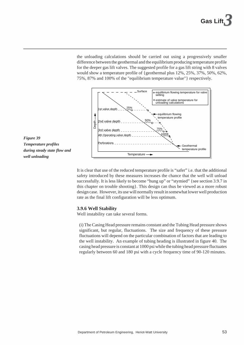
Department of Petroleum Engineering, Heriot-Watt University 53
33Gas Lift
the unloading calculations should be carried out using a progressively smallerdifference between the geothermal and the equilibrium producing temperature profilefor the deeper gas lift valves. The suggested profile for a gas lift string with 8 valveswould show a temperature profile of {geothermal plus 12%, 25%, 37%, 50%, 62%,75%, 87% and 100% of the "equilibrium temperature value"} respectively.
Temperature
Dep
th
25%
50%
75%
100%
1st valve depth
4th Operating valve depth
PerforationsGeothermaltemperature profile
equilibrium flowingtemperature profile
Surface equilibrium flowing temperature for valvesetting
estimate of valve temperature forunloading calculations
2nd valve depth
3rd valve depth
It is clear that use of the reduced temperature profile is “safer” i.e. that the additionalsafety introduced by these measures increases the chance that the well will unloadsuccessfully. It is less likely to become “hung up” or “stymied” {see section 3.9.7 inthis chapter on trouble shooting}. This design can thus be viewed as a more robustdesign case. However, its use will normally result in somewhat lower well productionrate as the final lift configuration will be less optimum.
3.9.6 Well StabilityWell instability can take several forms.
(i) The Casing Head pressure remains constant and the Tubing Head pressure showssignificant, but regular, fluctuations. The size and frequency of these pressurefluctuations will depend on the particular combination of factors that are leading tothe well instability. An example of tubing heading is illustrated in figure 40. Thecasing head pressure is constant at 1000 psi while the tubing head pressure fluctuatesregularly between 60 and 180 psi with a cycle frequency time of 90-120 minutes.
Figure 39
Temperature profiles
during steady state flow and
well unloading

54
.eru
sser
Pgni
buTdnagnisaCfognidroce
Rne
Pni
w T
DATE ON
DATE ON
TIME
TIME
AM
AM
11PM
MID
NIG
HT
1AM
2AM
3AM
4AM5AM6AM
7AM
8AM
9AM
10A
M11
AM
MID
DAY
1PM
2PM
3PM
4PM5PM 6PM
7PM
8PM
9PM
10PM
Liquid flow rate 1300 stb/dFlow rate gas 630 Mscf/dWater cut 98%Cycle frequency 90 - 120 minGas injection rate 350 Mscf/dWell depth 3500ft Vertical well
Well detailsTubing Head Pressure : 60 - 180 psi
Casing Head Pressure : 1020psi
(ii) Both the Tubing Head and the Casing Head Pressure show regularly fluctuatingvalues.
Professor Asheim of Trondheim University defined two parameters (F1 and F2)which can be used to determine whether a stable flow condition exists in either thetubing or casing / tubing annulus respectively. He showed that unstable flowconditions have to exist in both flow conduits before the overall well behavior isunstable.
The tubing (F1) parameter considers whether the changes in tubing inflow and gas
injection pressure resulting from chance fluctuations in the tubing head pressure willtend to die away and return the well to the current producing conditions (the definitionof stable flow). Thus a stable well condition (F
1 > 1) requires that a momentary
decrease in the downhole pressure will result in a greater influx of (high density)formation fluids relative to that of (low density) injection gas. The combination ofthese extra inflows result in a relative increase in the average tubing density,counteracting the original, momentary decrease in downhole pressure. The well isthus flowing with a stable condition since it tends to return to the original operatingcondition. By contrast, unstable flow (F
1 < 1) would have resulted in the well moving
to a different operating point. This stability criterion is equivalent to that discussedin Chapter 1 for naturally flowing wells.
The casing / tubing annulus (F2) parameter reflects the response of the flow of casing
gas to momentary fluctuations in the Tubing Pressure opposite the operating valvewhen the tubing flow is potentially unstable (F
1 < 1). Thus the well is unstable (F
2 < 1)
if a momentary decrease in downhole tubing pressure causes the casing pressure todecrease more slowly than the tubing pressure. The resulting increased pressure dropacross the gas lift valve will lead to a greater inflow of lift gas, providing the valve isnot “choked”. This would tend to decrease the bottom hole pressure further - movingthe well even further from its previous operating point.
Figure 40
Example of tubing heading

Department of Petroleum Engineering, Heriot-Watt University 55
33Gas Lift
Well stability can be improved by instituting choke control of the casing gas injectionpressure. It is more difficult for the well to show unstable behavior when the pressuredrop across the surface choke controlling the gas injection rate is greater than thepressure drop across the downhole operating valve. This arrangement prevents thegas flowing out of the casing annulus and into the tubing at a faster rate than it is beingreplaced by the lift gas supply to the well. {The inclusion of any extra pressure dropin the gas lift supply system will often decrease the maximum well production rate.}
Practical considerations will often result that, if a well is suffering from unstablebehavior, an operator will find it easier to adjust the surface choke rather than thechange the size of the operating valve’s downhole orifice. The pressure drop acrossthe surface choke may thus become the greater pressure drop; resulting in greatertendency for annulus heading (the reverse of what was being attempted). Amomentary drop in tubing press can then result in an excessive gas flow rate throughthe downhole orifice. There will be a delay in the pressure reduction being felt at thesurface, due to the large annular volume and high gas compressibility. The lift gassupply will not increase quickly enough to compensate for this pressure reductionsufficiently, particularly when its supply is being impeded by a small surface choke.The pressure at the bottom of the annulus will continue to drop - eventually the fallingcasing pressure will reduce the gas supply to the tubing. Once again, there will be adelay in the response of the surface choke and it will continue to supply excess gas,leading to a build up in the annulus pressure. These pressure excursions can berepeated regularly - the size and frequency of the fluctuations depending on theparticular well circumstances.
One further cause of casing and tubing head pressure fluctuations is valve multi-pointing. This occurs when more than one valve is passing gas i.e. gas is being injectedinto the tubing at several different levels. This can represent an apparently stablesituation from the point of view of the Tubing and Casing Head pressures. Howeverfluctuations may also be induced by one valve repetitively opening and closing dueto the temperature changes induced by the changing flow conditions.
3.9.7 Dual Gas LiftThe most common dual gas lift configurations are two strings of 2.375in or 3.5 in ODtubing run inside 7.0 or 9.635 in OD casing respectively. Combinations of other sizesor even concentric strings are feasible, but rarely used.
The first problem with Dual Gas Lift completions is the well completion operationitself - there is insufficient width for the gas lift mandrels in the two strings to pass oneanother. This is overcome by designing the spacing of the mandrels in the two tubingstrings and the dual tubing running procedure so that the gas lift mandrels do not needto pass one another during the well completion operation.
A well with a Dual gas Lift Completion can be treated as a normal single completionif only one tubing string requires gas lift. The difficulty arises in ensuring a properdistribution of the lift gas between the strings if both strings are to be gas lifted i.e. onestring may take most of the gas while the second tubing is starved of gas.
One solution to prevent the valves in the different strings interfering with the operationof the other one is to install valves with significantly different operating characteristics

56
in the different strings. e.g. One string uses IPO valves while TPO valves are installedin the second string. The gas allocation between the strings is then controlled by theselection of the chokes installed in the operating valves. An alternative solution is toinstall TPO valves in both strings, since they do not respond strongly to the annuluspressure. However, practical experience shows that multipointing is a commonoccurrence for this design.
3.9.8 Trouble ShootingInefficient gas lift operation can be caused by:
(i) Inflow Problems due to:
(a) Incorrect size of choke (too large or too small),
(b) Incorrect lift gas (casing) pressure (too high or too low),
(c) Fluctuating compressor lift gas pressures and
(d) Incorrect lift gas flow rate (too high or too low).
(ii) Outlet Problems can include:
(a) Inadequate or restricted (due to partial plugging) gas flow through theoperating valve,
(b) Increased hydrostatic gradient across tubing due to increasing water cut andconsequent reduction in the produced fluid’s “natural” gross Gas Oil Ratio and
(c) The wellhead choke not having been fully opened or the separator pressurebeing set too high.
(iii) Downhole Problems. These include:
(a) A hole in the tubing and the
(b) Incorrect operation of valves due to either:
(i) Mechanical problems with the valve operation itself,
(ii) Wrong pressure setting of the gas lift valve’s nitrogen charge or
(iii) Incorrect gas lift valve spacing in the tubing string.
3.9.9 Trouble Shooting TechniquesOperational problems will be resolved most quickly by carrying out a systematicinvestigation to identify the fundamental cause of sub-optimum production from a gaslifted well. The analysis techniques used and the data gathered should include the:
(i) (Computer) modeling of annulus and tubing pressure profile.

Department of Petroleum Engineering, Heriot-Watt University 57
33Gas Lift
(iii) Comparison with a flowing temperature and pressure survey.
(iv) Carrying out a production test with multi gas injection rates.
(v) Performing of an analysis of the historical well test and production data toidentify trends.
(vi) Carrying out an echometer survey to identify the fluid level in the casing /tubing annulus. The echometer is an acoustic device which measures the transit timefor a signal generated at the surface to travel down the annulus and be reflected backto the surface from the liquid level in the casing / tubing annulus. This timemeasurement can be translated into a depth if the acoustic velocity is known.
3.9.10 Some Field Examples of operational problems:
(i) Injection pressure rises to its maximum value while the injection rate drops tozero. This indicates that an upper value closed before the lower valve opened i.e. thegas injection point has not being passed to successively deeper gas lift valves. Thewell is “stymied” or “hung up” and the setting on one or more gas injection valvesneeds to be changed.
(ii) Casing head pressure fluctuates by 5 to 10 psi but the gas injection rate isconstant. The injection point is being transferred between two valves (one form ofvalve multi- pointing).
(iii) Casing head pressure fluctuates by 10-20 psi while the injection rate is alsochanging. This suggests that a lower valve is opening and closing while a second,higher valve is continually open.
It should be remembered that it is always possible that the problem is more apparentthan real i.e. the accuracy of the flow meters (in particular) and pressure gauges needsto be verified. Once it has been confirmed that the flow and pressure measurementsare correct, then one can adjust the lift gas injection rate to the casing or increase theflowing tubing head pressure by closing the surface choke. These changes can rectifythe problem, though frequently the cause is a valve problem (mechanical damage orincorrect setting) which can only be solved by its replacement i.e. a wireline wellintervention is required.
3.10 FIELD PRODUCTION OPTIMISATION
We have already discussed how to maximise the production of gas lifted for a singlewell. This involved the development of (theoretical) (computer) model of the singlewell’s performance and its calibration against the actual well data via carrying outmulti-rate well tests. (This aspect of managing Oil and Gas Field Operations iscovered in greater detail in chapter 10 of this Production II module). A calibratedmodel will allow those parameters controlled from the surface {injection gas chokesetting, injection gas pressure and separator pressure} to be set to their optimumvalues. This process requires the systematic collection, verification, storage and

58
analysis of the field data since the (computer) model of the well can never be moreaccurate than the data against which the model was calibrated.
The individual well performance models for the wells in the field should now becombined to give a total field model so that the field performance can be maximisedagainst the relevant constraints. These constraints can either be:
(i) Physical constraints imposed by the overall system e.g. the total, available lift gasinjection rate, the volume of water that can be handled by the separation system, the(net) oil production from wells producing from different reservoirs may have to bemixed in a certain ratio to ensure that the specified crude oil quality is maintained.
(ii) Individual wells or reservoir specific constraints e.g. certain wells may have tobe produced at a specified minimum rate for reservoir management purposes.
The task is then to maximise the NPV operating cash income over the life of the wells.This normally equates to maximising the oil production by ranking each individualwell’s optimum production response to incremental gas injection. This concept isexplained in figure 41, where the net oil production (or revenue) is plotted against thelift gas injection rate (or production cost). A minimum (or “kick-off”) lift gas injectionrate, (V
1) is required to bring the well on production at the initial production rate Q
1.
The well performance curve is then plotted so that the incremental productionincrease, (∆Q
n) can be evaluated for equal increments in the lift gas injection rate,
(∆xn). It can be seen that the incremental GUF {Gas Utilisation Factor or (∆Q
n / ∆x
n)}
decreases as the lift gas injection rate increases. In fact, the GUF represents the slopeof the well performance curve (see Figure 41). This slope is also related to the factor:
{incremental (net oil) production revenue} {incremental (gas lift & other production) costs}
Maximumproduction
Net
oil
prod
uctio
n or
rev
enue
Lift - gas injection rate
Q1
V1
V1 "Kick - off" lift gas injection rate
Q1 Initial oil at "kick - off"
∆xn Equal lift gas rate increments
∆Qn Corresponding incremental oilproduction or revenue.
GUFn Gas Utilisation Factor
Economic limit
∆x1
∆x2∆Q1
∆x3∆Q2
∆x4∆Q3
∆x5∆Q4
∆x6
∆x7
∆x8∆x9 ∆x10
Economic limit where marginal(net production) revenue equalsmarginal lifting costs.
*
*
GUF1
GUF7
GUF4
This factor is plotted against the gas injection rate in figure 42. The economic limitand the technical maximum oil production are the points at which this factor equals
Figure 41
The incremental gas
utilisation factor decreases
with increasing gas
injection rate

Department of Petroleum Engineering, Heriot-Watt University 59
33Gas Lift
1.0 and 0 respectively.
2.5
2.0
1.5
1.0
0.5
0
Lift gas injection rate
Incr
emen
tal (
Rev
enue
/ C
osts
)Economic limit where incrementalcosts = incremental revenue
x 1 x 2 x 3 x 4 x 5 x 6 x 7 x 8 x 9 x 1 0 x 1 1 x 1 2
Technical maximum production
"Kick - off" gasinjection rate
Lift gasincrements∆ ∆ ∆ ∆ ∆ ∆ ∆∆ ∆ ∆ ∆ ∆
Allocation of the available lift gas between wells is performed by comparing the GUFvalues. This calculation is complicated by the:
(i) Varying well “kick-off” gas requirements (figure 43 shows three wells exhibitingdifferent “kick-off” behavior).
(ii) Reservoir and well specific constraints, as well as any other production systemconstraints which also have to be honored.
(iii) The numbers of wells involved (large gathering systems can connect more than1000 production wells).
Net
oil
prod
uctio
n ra
te
Lift - gas injection rate
Nat
ural
flow
(wel
l a )
Well a
Well b
Well c
KOGcKOGb
Initial Gas Utilisation Factors
KOGb, KOGc = "Kick - off" lift - gasrequired by wells b and c.
Specialist software packages e.g. FieldfloTM, NetOptTM etc. are available from anumber of vendors which are capable of optimising such large systems. However, itmust always be borne in mind that the optimised production recommendation resultswill only be as good as the input field data. Once again, this points to the need to ensurethat a systematic data collection, validation and management system is installed at thesame time as such optimisation packages are purchased.
Figure 43
Well performance curves
for three wells
Figure 42
Gas lift incremental cost
curve.
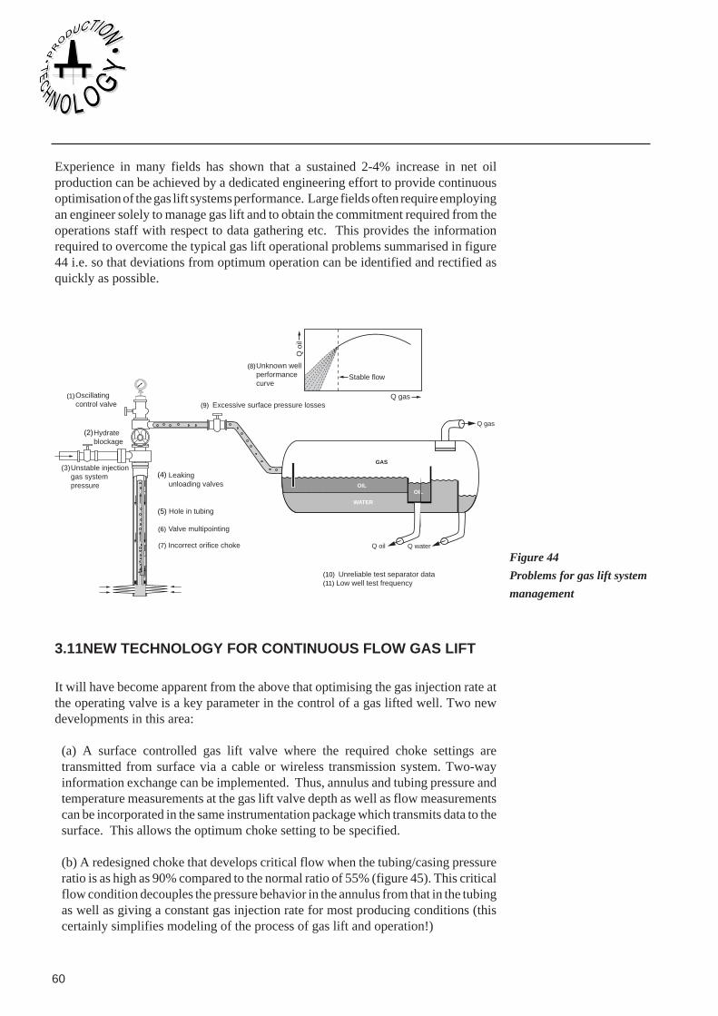
60
Experience in many fields has shown that a sustained 2-4% increase in net oilproduction can be achieved by a dedicated engineering effort to provide continuousoptimisation of the gas lift systems performance. Large fields often require employingan engineer solely to manage gas lift and to obtain the commitment required from theoperations staff with respect to data gathering etc. This provides the informationrequired to overcome the typical gas lift operational problems summarised in figure44 i.e. so that deviations from optimum operation can be identified and rectified asquickly as possible.
OIL
WATER
GAS
Q o
il
Q gas
Stable flow
Unknown wellperformancecurve
Leakingunloading valves
Hole in tubing
Unstable injectiongas systempressure
(10) Unreliable test separator data(11) Low well test frequency
(9) Excessive surface pressure lossesOscillatingcontrol valve
Hydrateblockage
Valve multipointing
Incorrect orifice choke
OIL
(1)
(6)
(2)
(4)(3)
(5)
(7)
(8)
Q waterQ oil
Q gas
3.11NEW TECHNOLOGY FOR CONTINUOUS FLOW GAS LIFT
It will have become apparent from the above that optimising the gas injection rate atthe operating valve is a key parameter in the control of a gas lifted well. Two newdevelopments in this area:
(a) A surface controlled gas lift valve where the required choke settings aretransmitted from surface via a cable or wireless transmission system. Two-wayinformation exchange can be implemented. Thus, annulus and tubing pressure andtemperature measurements at the gas lift valve depth as well as flow measurementscan be incorporated in the same instrumentation package which transmits data to thesurface. This allows the optimum choke setting to be specified.
(b) A redesigned choke that develops critical flow when the tubing/casing pressureratio is as high as 90% compared to the normal ratio of 55% (figure 45). This criticalflow condition decouples the pressure behavior in the annulus from that in the tubingas well as giving a constant gas injection rate for most producing conditions (thiscertainly simplifies modeling of the process of gas lift and operation!)
Figure 44
Problems for gas lift system
management

Department of Petroleum Engineering, Heriot-Watt University 61
33Gas Lift
Critical flow (Nova “) valves
Critical flow region Sub - criticalflow region
P tubing≈55% P casing
P tubing≈90% P casing
P casing
Tubing pressure (psi)
Conventional port valve
Gas
inje
ctio
n ra
te (
MM
scf/d
)
(c) Coiled Tubing based Gas Lift Completions in which gas lift values and mandrelscan be incorporated as an integral part of a coiled tubing string. These can beemployed in two manners:
(a) To replace the conventional production tubing (Figure 46). This particularcompletion was designed to test an exploration or appraisal well.
1" gas lift valve in 2.375" mandrel
1.75" coiled tubing
Orifice valve in 2.375" mandrel
Locator / seal assembly
Polished bore receptacle
9.625" casing shoe
18.625" casing shoe
30" casing shoeSurface controlled subsurfacesafety valve (SCSSSV)
Producing formation
Perforations
7" liner shoe
Production to separator
Lift gas
Figure 45
Orifice valve performances
compared
Figure 46
Gas lift completion where
coiled tubing has replaced
the tubing string

62
(b) As a second production string within an existing tubing (Figure 47). This allowsgas lift to be introduced to aid well production without having to mobilise a drillingrig to recomplete the well. This does however require that a polished bore receptacle,into which the coiled tubing seal assembly can be located, has included in the originaltubing string. The advantage of this approach is that it is probably the cheapestmethods of installing gas lift in a well where the casing integrity has been lost.
Producing Formation
Perforations
Gas lift valve mountedin mandrel
Surface Controlled SubsurfaceSafety Valve ( SCSSSV)
Control line hanger
Coiled tubing hanger
Control line for SCSSSV
2" coiled tubing
Orifice
Locator seal assembly
Polished bore receptacle
Gas injection to tubing/ coiled tubing annuls
Production to separator
(c) Alternatively, the orifice valve can be omitted with the coiled tubing suspendedfrom its hanger - the gas injection taking place via the coiled tubing’s open end.
3.12 INTERMITTENT GAS LIFT
All the above has discussed continuous flow gas lift. The intrinsic flexibility of thegas lift concept allows it to be adapted to a wide range of situations; however it doesbecome inefficient at low formation fluid inflow rates (<150 bf/d with a 2.375 in ODtubing rising to < 300 bf/d for a 3.5 in OD tubing). A partial answer to the problemis intermittent lift where the gas is switched on for a short period of time at regularintervals :
Figure 47
A coiled tubing inner
production string

Department of Petroleum Engineering, Heriot-Watt University 63
33Gas Lift
(i) The formation fluid level in the tubing increases during the periods that the gaslift is switched off.
(ii) The formation fluid that has collected above the valve is lifted out during a periodof lift gas injection.
(iii) The flow of lift gas to the well is halted and the cycle is repeated.
A time cycle controller opens the surface lift-gas valve for a predetermined time atregular intervals and then shuts it. The process typically produces some 2-5 bbls liquidper cycle with a frequency of 1-3 cycles per hour (Figure 48). The valve spread (ordifference between pressure needed to open and close the valve - see section 3.7.2)controls the minimum amount of gas used during each intermittent gas lift cycle.
.eru
sser
Pgni
buTdnagnisaCfognidroceR
neP
niw T
DATE ON
DATE ON
TIME
TIME
AM
AM
5AM
6AM
7AM
8AM
9A
M
10AM
11AMMIDDAY 1PM
2PM
3PM
4PM
5PM
6PM
1000
800
600
400
300
200
100
500
700
900
400300
200100
5
1000
800
600
400300
200100
500
700
900
00 00 00 400
300
200
100
500
00010
00
800
600
400
300
200
100
500
700
900
1000
800
600
400
300
200
100
500
700
900
Wellhead Pressure
Casing Pressure
Cycle time 30 minInjection time 2 minProduction rate 144 bfpdInjection gas rate 350 M scf/d
Well details
This approach is more efficient in terms of the volume of gas required to lift a givenvolume of liquid than continuous gas lift for these low rate wells. However, it stillrequires relatively high gas volumes due to the fall back of the liquid (of the order of10% of the tubing volume) present in the tubing at the time when the gas is switchedoff. This inefficiency can be removed by incorporating a plunger to displace all theliquid to the surface, the plunger itself having been displaced up the tubing by injectinglift gas underneath {see figure 6(e)}. The process is as follows:
(i) The plunger displaces the fluids that have entered the well during the period thatthe lift gas was shut off.
(ii) The flow of lift gas is halted once the plunger reaches the wellhead and the cyclerepeated.
This process is also known as Plunger Assisted Intermittent Lift (PAIL) or chamberlift. PAIL has particular advantages when the well is suffering from severe waxdeposition since the regular passage of the plunger ensures the tubing remains clearof wax.
Figure 48
Intermittent gas lift

64
3.13 GRAPHICAL GAS LIFT DESIGN EXERCISE FOR WELLEDINBURGH-2
3.13.1 Introduction
The earlier section in this chapter have showed how the well production wasinfluenced by parameters such as the gas injection rate, tubing size, depth of gasinjection, and flowing tubing head pressure etc. This sensitivity study can be used todetermine the optimum gas lift completion design parameters. It is now necessary tospace out the unloading valves so that the gas can reach the operating valve at the depthshown above. The procedure used will be illustrated by using the Edinburgh-2 wellas an example (see Table 7 for well design conditions).
Gas injection pressure 1250 psig
Gas injection rate 500 M scf/d
"Kill" brine density 0.465 psi / ft
Depth mid perforations 10,000 ft
Reservoir pressure 3600 psi
(Gross fluid) Production index 0.5 bf/d/psi
Water cut 65% vol.
Oil density 35 API or 0.37 psi/ft
Production water density 1.05 g/cm3 or 0.455 psi/ft
( Average) produced fluid density 0.426 psi/ft
(relative) gas gravity 0.6
Flowing wellhead pressure 100 psi
Average flowing gradients: For producing well
250 bf/d at GLR of 2105 scf/b 0.07 psi/ft
500 bf/d at GLR of 1105 scf/b 0.1psi/ft
750 bf/d at GLR of 770 scf/b 0.157 psi/ft
800 bf/d at GLR of 730 scf/b 0.18 psi/ft
Table 7
Well Edinburgh - 2 gas lift
design conditions

Department of Petroleum Engineering, Heriot-Watt University 65
33Gas Lift
Pressure (psi)
Dep
th (
ft)
1000
2000
3000
4000
5000
6000
7000
8000
9000
10,000
500 1000 1500 2000 2500 3000 3500Pressure (psi)
500 1000 1500 2000 2500 3000 3500
Static (kill) brine gradient
0.465 psi / ft
Reservoirpressure3600 psi
2260 ft
1600 psi surface gas injection pressure
1200 surface psi gas injection pressure
800 psi surface gas injection pressure
500 psi surface gas injection pressure
Gas SG = 0.6Gas SG = 0.8
Equilibrium
level
kill brine
600
0.08
0.9 Gas S.G.
0.8 Gas S.G.
0.7 Gas S.G.
0.6 Gas S.G.
0.07
0.06
0.05
0.04
0.03
0.02
0.01700 800 900 1000 1100 1200 1300 1400 1500
Gas
Gra
dien
t, ps
i/ft.
Surface Gas Injection Pressure (psig)
T = 70ºF at Surface190ºF at 10000 ft TVD
Figure 49b
Initial conditions for
"killed" well
Figure 49a
Injection gas gradients for
well Edinburgh 2

66
3.13.2 Initial Conditions - the “Dead” WellThe well has been completed and circulated to a “kill” brine of density 0.465 psi/ft.Figure 49 shows that the reservoir pressure is only sufficient to support the fluid levelin tubing and tubing/casing annulus to a depth of 2258 ft. Gas pressure gradients forvarious gas injection pressures have been drawn. The effect of using gases of differentrelative densities (0.6 and 0.8) for the 1200 psi surface pressure case has also beenincluded.
3.13.3 Construction of the “Equilibrium Curve”The range of production rates achievable using gas lift and the required gas injectiondepths must be calculated first. A nodal analysis calculation is carried out for aproduction rate of 500 b/d using a gas lift injection point at depth D ft as the node andthe data from Table 7.
Calculation from Surface
Pressure at gas injection point = separator pressure + 0.1 D
Calculation from Reservoir:
Pressure at gas injection point = Reservoir Pressure - drawdown - 0.426* (10000 - D)
* We have assumed that the frictional pressure losses below the gas lift valve arenegligible at this low flow rate.
These two pressures are equal and thus :
D = 5400 ft and the gas injection pressure at this depth is 640 psi.
The latter corresponds to a surface gas pressure of 560 psi. The same calculation canbe carried out for gross production rates ranging from 250 to 800 b/d - see Table 8 andfigure 50. (Remember that the flowing pressure gradient has to be changed as well asthe drawdown for each calculation.) This table shows that gas injection pressuresranging from 350 psi to 1825 psi are required. It would not be realistic to use a constantgas density for calculating the surface pressure for this wide range of conditions. Theinjection gas pressure gradient is also dependent on the average pressure. Table 8includes an approximate value which allows us to estimate the surface gas injectionpressure required. A more accurate value could have been calculated using theequation given in section 3.8.4.
Production rate (bf/d) 250 500 750 800
Gas injection depth (ft) 3540 5400 8400 9594
Gas injection pressure at gas lift valve (psi) 348 640 1419 1827
Average gas gradient at this pressure (psi/ft) 0.01 0.015 0.03 0.045
Required surface gas injection pressure (psi) 313 560 1167 1395
Table 8
Calculation of "The
Equilibrium Curve"

Department of Petroleum Engineering, Heriot-Watt University 67
33Gas Lift
Pressure (psi)
Dep
th (
ft)1000
2000
3000
4000
5000
6000
7000
8000
9000
10,000
500 1000 1500 2000 2500 3000 3500Pressure (psi)
500 1000 1500 2000 2500 3000 3500
The "Equilibrium
Inflow / O
utflow C
urve"G
as gradients SG
= 0.6
313560
11671395
Surface gas injection pressures (psi)
Reservoirpressure800 bf/d
750 bf/d
500 bf/d
250 bf/d
Figure 50 summarises the producing conditions which simultaneously satisfy thereservoir inflow and tubing outflow conditions. This line is called the “EquilibriumCurve”. It allows a quick estimate of the depth, and associated pressures, at which theoperating valve must be installed to achieve a given production rate. As expected, thehighest production rates are achieved with the deepest gas injection. The available gaslift pressure is 1250 psi (Table 7) - hence we will set a target production rate of 750bf/d for the Edinburgh -2 gas lift completion by installing the operating valve at 8400ft. It now needs to be confirmed that the well can be unloaded when completion brine(of density 0.465 psi/ft) is present in the well.
Figure 50
Construction of "The
equilibrium curve"

68
Pressure (psi)
Dep
th (
ft)
1000
2000
3000
4000
5000
6000
7000
8000
9000
10,000
400 800 1200 1600 2000 2400 2800Pressure (psi)
Injection gas gradient
Surface gas injection pressure (1250 psi)
400 800 1200 1600 2000 2400 2800
Flowing wellhead pressure
100 psi
Operating valve at 8400 ft Produced fluid
(750 bpd) gradient
= 0.426 psi / ft1500 psi drawdownrequired to produce750 bf/d
Valvenumber1
Kill brine gradient
0.465 psi / ft
2530 ft
750 bpd produced fluid + 500 MM
scfd
injection gas = 0.15 psi / ft
"The Objective G
radient"
50 psi safety margin
3.13.4 The Unloading ProcessThe unloading calculation is begun by calculating the flowing bottom hole pressure(2100 psi) required to produce 750 bf/d. The pressure profile for the flowing well isthen constructed from this point to the surface wellhead pressure (100 psi) using theflowing fluid gradients before (0.426 psi/ft) and after gas injection (0.15 psi/ft). Thisline is known as the “Objective Gradient” (Figure 51). The flowing gradients havebeen represented here as straight lines to simplify the calculations. The intersectionof these two lines is the depth at which the operating valve will be installed (8400 ft).Also shown is the intersection between a (static) brine gradient drawn from the(flowing) wellhead pressure of 100 psi to the gas gradient line for a surface pressureof 1200 psi. This pressure is 50 psi less than the nominal gas lift system operatingpressure of 1250 psi. The lower value is as an additional safety margin to ensure thatthe gas lift completion will still unload despite fluctuations in the compressor output
Figure 51
Well unloading stage 1,
maximum depth of first gas
lift valve

Department of Petroleum Engineering, Heriot-Watt University 69
33Gas Lift
pressure. It also compensates for any frictional pressure loss due to gas flow acrossthe valve.
The intersection between the gas and brine gradient lines is at 2530 ft - this is the depthat which the first unloading valve should be placed (Figure 51). The surface gaspressure is sufficient to displace the brine from the annulus into the tubing and out ofthe well.
Pressure (psi)
Dep
th (
ft)
1000
2000
3000
4000
5000
6000
7000
8000
9000
10,000
400 800 1200 1600 2000 2400 2800Pressure (psi)
400 800 1200 1600 2000 2400 2800
100
Operating valve at 8400 ftProduced fluid
(750 bpd)
= 0.426 psi / ft
1500 psi drawdownrequired to produce750 bf/d
Valvenumber1
Injection gas gradient
Surface gas injection pressure (1250 psi)Flowing wellhead pressure
Valvenumber2 4485 ft
2530 ft
Brine gradient
reducing under
the influence
lift gas injection
Brine gradient
"The objective gradient"
Gas injection reduces densityof brine above first gas lift valve.
50 psi safety margin
The gas will now enter the tubing via the gas lift valve and reduce the pressure exertedby the fluid in the tubing above the valve. This reduced pressure also ensures that the
Figure 52
Well unloading stage 2,
depth selection for 2nd gas
lift valve

70
pressure in the annulus remains greater than that in the tubing at all depths. Hence fluidcontinues to be displaced from the annulus into the tubing through the second andlower valves. This process is illustrated in figure 52 where it is shown how the brinedensity is reduced under the influence of lift gas injection until it reaches the“Objective Gradient”. The depth (4485 ft) at which the completion brine gradientintersects the gas gradient line is the maximum depth at which the second unloadingvalve can be placed.
Pressure (psi)
Dep
th (
ft)
1000
2000
3000
4000
5000
6000
7000
8000
9000
10,000
400 800 1200 1600 2000 2400 2800Pressure (psi)
400 800 1200 1600 2000 2400 2800
Operating valveat 6650 ft
Produced fluid
gradient
1070 psi drawdownrequired to produce535 bf/d
Valvenumber1
Injection gas gradient
Surface gas injection pressure (1250 psi)Flowing wellhead pressure
50 psi safety margin
2530 ft
The objective gradient
2
3
4
56
100 psi safety margin
150 psi safety margin
200 psi safety margin250 psi safety margin
2530
2530 ft
1750 ft
1200 ft
750 ft
400 ft
200 ft}
100
Valve spacing
6850 ft6650 ft
6250 ft
5500 ft
4300 ft
50 psi safety margin
Classical design procedures assume that the upper valve shuts immediately the gasreaches a lower valve. Section 3.7.3, which described valve performance, showed that
Figure 53
Well unloading stage 3,
inclusion of safety margins
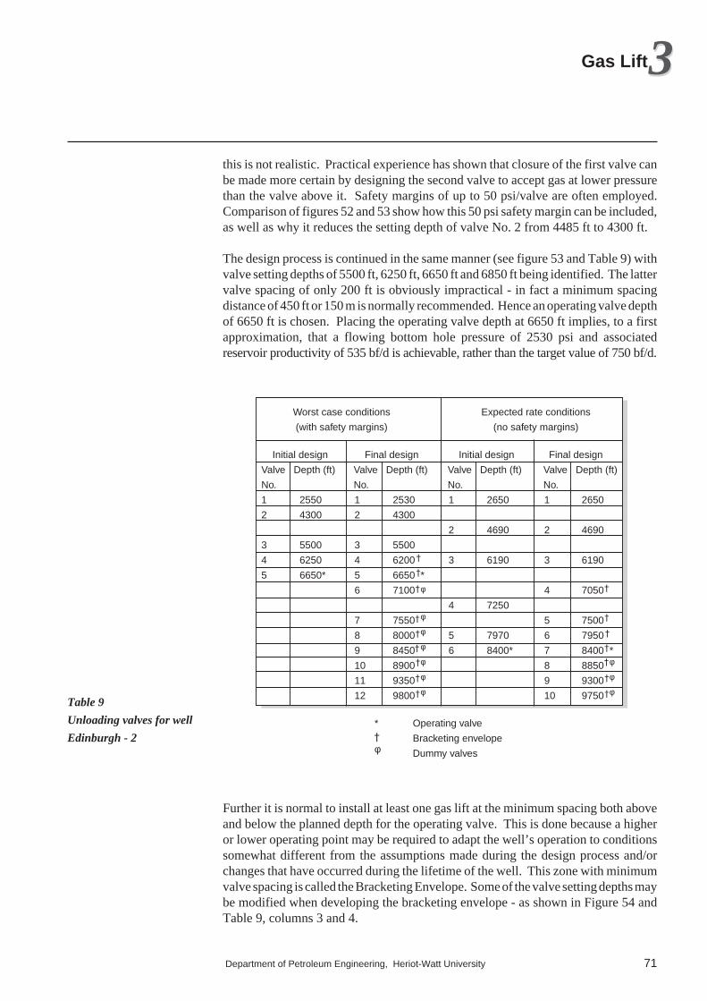
Department of Petroleum Engineering, Heriot-Watt University 71
33Gas Lift
this is not realistic. Practical experience has shown that closure of the first valve canbe made more certain by designing the second valve to accept gas at lower pressurethan the valve above it. Safety margins of up to 50 psi/valve are often employed.Comparison of figures 52 and 53 show how this 50 psi safety margin can be included,as well as why it reduces the setting depth of valve No. 2 from 4485 ft to 4300 ft.
The design process is continued in the same manner (see figure 53 and Table 9) withvalve setting depths of 5500 ft, 6250 ft, 6650 ft and 6850 ft being identified. The lattervalve spacing of only 200 ft is obviously impractical - in fact a minimum spacingdistance of 450 ft or 150 m is normally recommended. Hence an operating valve depthof 6650 ft is chosen. Placing the operating valve depth at 6650 ft implies, to a firstapproximation, that a flowing bottom hole pressure of 2530 psi and associatedreservoir productivity of 535 bf/d is achievable, rather than the target value of 750 bf/d.
Initial design Final design Initial design Final design
Valve Depth (ft) Valve Depth (ft) Valve Depth (ft) Valve Depth (ft)
No. No. No. No.
1 2550 1 2530 1 2650 1 2650
2 4300 2 4300
2 4690 2 4690
3 5500 3 5500
4 6250 4 6200 3 6190 3 6190
5 6650* 5 6650 *
6 7100 φ 4 7050
4 7250
7 7550 φ 5 7500
8 8000 φ 5 7970 6 7950
9 8450 φ 6 8400* 7 8400 *
10 8900 φ 8 8850 φ
11 9350 φ 9 9300 φ
12 9800 φ 10 9750 φ
* Operating valve
Bracketing envelopeφ Dummy valves
Expected rate conditions
(no safety margins)
Worst case conditions
(with safety margins)
Further it is normal to install at least one gas lift at the minimum spacing both aboveand below the planned depth for the operating valve. This is done because a higheror lower operating point may be required to adapt the well’s operation to conditionssomewhat different from the assumptions made during the design process and/orchanges that have occurred during the lifetime of the well. This zone with minimumvalve spacing is called the Bracketing Envelope. Some of the valve setting depths maybe modified when developing the bracketing envelope - as shown in Figure 54 andTable 9, columns 3 and 4.
Table 9
Unloading valves for well
Edinburgh - 2

72
Pressure (psi)
Dep
th (
ft)
1000
2000
3000
4000
5000
6000
7000
8000
9000
10,000
400 800 1200 1600 2000 2400 2800Pressure (psi)
400 800 1200 1600 2000 2400 2800
Actual operating valve
Produced fluid
1500 psi drawdownrequired to produce750 bf/d
Valvenumber1
Injection gas gradients
Surface gas injection pressure (1250 psi)Flowing wellhead pressure
50 psi safety margin
2530 ft
The objective gradient
2
3
4
5
6
100 psi safety margin
2530
7
8
9
10
11
12
Extendedbracketingenvelope.
150 psi safety margin6200 ft
6650 ft
7100 ft
Target operating valve depth
The bracketing envelope
1070 psi drawdownrequired to produce535 bf/d
100
4300 ft
5500 ft
50 psi safety margin
In addition, it is shown that the:
(i) bracketing envelope has been extended in the final design as far as the bottomof the well to allow deep gas lift if the reservoir pressure / well productivity decreasesufficiently. This worst case design requires 12 gas lift valves to be installed withthe operating valve placed at 6650 ft and dummy valves installed in the bottom 7mandrels.
(ii) 50 psi safety margin used between each succeeding valve has created a robustdeign with high confidence that the well will unload to a depth of 6650 ft.
(iii) depth for the operating valve is shallower than the target depth of 8400 ft. Thisreduces the well production to 535 bf/d, lower than the target value of 750 bf/d.
Figure 54
Final design: worst case
conditions

Department of Petroleum Engineering, Heriot-Watt University 73
33Gas Lift
By contrast, the target fluid production can be achieved if an “expected rateconditions” design is made (Figure 55 and Table 9). The final design shownincorporates the modifications made due to introduction of the “Bracketing Enve-lope” concept. It:
(i) uses two fewer gas lift valves.
(ii) achieves the target production rate of 750 bf/d.
(iii) depends for its success on the well conditions being exactly as prognosed. Thisis required to ensure that the unloading process works efficiently.
Pressure (psi)
Dep
th (
ft)
1000
2000
3000
4000
5000
6000
7000
8000
9000
10,000
400 800 1200 1600 2000 2400 2800Pressure (psi)
400 800 1200 1600 2000 2400 2800
1500 psi drawdownrequired to produce750 bf/d
Valvenumber1
Injection gas gradient
Surface gas injectionpressure (1250 psi)
Flowing wellhead pressure
4690 ft
2650 ft
2
3
4
5
6
6190 ft
7
8
9
Extendedbracketingenvelope.
7250 ft
9300 ft
9250 ft
7500 ft
8400 ftOperatingvalve
Recommended spacing
- 7050 ft
- 7950 ft
- 8400 ft
- 8850 ft
Finaldesign
"The Objective G
radient" for
750 bpd + 500 Msc f/d gas
7970 ft
2650 ft
2040 ft
1500 ft
1060 ft
720 ft
430 ft
Valve Spacing
The bracketingenvelope
Figure 55
Final design: expected rate
conditions

74
3.13.5 Gas Lift Optimisation Exercise
QuestionFigures 56 to 58 show the (gross) fluid production rate from three gas lifted wells. Thefollowing two exercises illustrate a procedure to manually allocate a limited volumeof gas (2 and 5 MM scf/d) so as to produce the maximum volume of oil.
6000
5600
5200
4800
4400
4000
3600
3200
2800 1 2 3 4 5 6
Gas injection rate (MM scf/d)
(Gro
ss fl
uid)
Pro
duct
ion
rate
(bf
/d)
Water cut = 25%
Figure 56
Gas lift performance - well 1

Department of Petroleum Engineering, Heriot-Watt University 75
33Gas Lift
1 2 3 4 5 6 Gas injection rate (MM scf/d)
(Gro
ss fl
uid)
Pro
duct
ion
rate
(bf
/d)
3200
2800
2400
2000
1600
1200
800
400
0
Water cut = 40%
1 2 3 4 5 6 Gas injection rate (MM scf/d)
(Gro
ss fl
uid)
Pro
duct
ion
rate
(bf
/d)
3200
2800
2400
2000
1600
1200
800
400
0
Gas Lift Performance - Well 3
Water cut = 45%
Figure 57
Gas lift performance - well 2
Figure 58
Gas lift performance - well 3
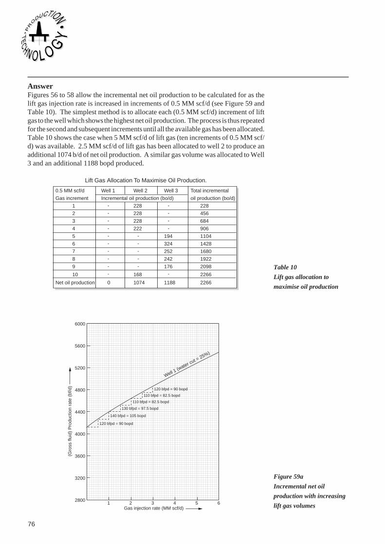
76
AnswerFigures 56 to 58 allow the incremental net oil production to be calculated for as thelift gas injection rate is increased in increments of 0.5 MM scf/d (see Figure 59 andTable 10). The simplest method is to allocate each (0.5 MM scf/d) increment of liftgas to the well which shows the highest net oil production. The process is thus repeatedfor the second and subsequent increments until all the available gas has been allocated.Table 10 shows the case when 5 MM scf/d of lift gas (ten increments of 0.5 MM scf/d) was available. 2.5 MM scf/d of lift gas has been allocated to well 2 to produce anadditional 1074 b/d of net oil production. A similar gas volume was allocated to Well3 and an additional 1188 bopd produced.
Lift Gas Allocation To Maximise Oil Production.
0.5 MM scf/d Well 1 Well 2 Well 3 Total incremental
Gas increment Incremental oil production (bo/d) oil production (bo/d)
1 228 228
2 228 456
3 228 684
4 222 906
5 194 1104
6 324 1428
7 252 1680
8 242 1922
9 176 2098
10 168 2266
Net oil production 0 1074 1188 2266
-
-
-
-
-
-
-
-
-
-
-
-
-
-
-
-
-
-
-
-
6000
5600
5200
4800
4400
4000
3600
3200
2800 1 2 3 4 5 6
Gas injection rate (MM scf/d)
(Gro
ss fl
uid)
Pro
duct
ion
rate
(bf
/d)
Well 1 (w
ater cut = 25%)
120 bfpd = 90 bopd
140 bfpd = 105 bopd
130 bfpd = 97.5 bopd
110 bfpd = 82.5 bopd
110 bfpd = 82.5 bopd
120 bfpd = 90 bopd
Figure 59a
Incremental net oil
production with increasing
lift gas volumes
Table 10
Lift gas allocation to
maximise oil production

Department of Petroleum Engineering, Heriot-Watt University 77
33Gas Lift
6000
5600
5200
4800
4400
4000
3600
3200
2800 1 2 3 4 5 6
Gas injection rate (MM scf/d)
(Gro
ss fl
uid)
Pro
duct
ion
rate
(bf
/d)
Well
2 (w
ater
cut =
40%
)
380 bfpd = 228 bopd
380 bfpd = 228 bopd
380 bfpd = 228 bopd
370 bfpd = 222 bopd
280 bfpd = 168 bopd
240 bfpd = 144 bopd
6000
5600
5200
4800
4400
4000
3600
3200
2800 1 2 3 4 5 6
Gas injection rate (MM scf/d)
(Gro
ss fl
uid)
Pro
duct
ion
rate
(bf
/d)
Well 3 (w
ater cut =
45%)
360 bfpd = 198 bopd
590 bfpd = 324.5 bopd
560 bfpd = 252 bopd
440 bfpd = 242 bopd
320 bfpd = 176 bopd
280 bfpd = 154 bopd
Figure 59b
Incremental net oil
production with increasing
lift gas volumes
Figure 59c
Incremental net oil
production with increasing
lift gas volumes

78
Table 10 shows that this calculation is not quite as simple as it appears due to the needfor a small volume of "Kick - off" gas to bring well 3 into production. This is illustratedwhen only 2 MM scf/d of lift gas is available. The simple approach used abovesuggests that it should all be allocated to Well 2 where it will recover an extra 906 bopd.However, allocating the same volume of gas to Well 3 will produce 1016 b/d of extranet oil (Table 11). This calculation illustrates why the slope of the curve (the GasUtilisation Factor) is a better optimisation factor rather than the simplistic incrementalproduction approach suggested above.
0.5 MMscfd Incremental oil production (bopd)
Gas increment Well 1 Well 2 Well 3
1 90 228 194
2 105 228 324
3 97.5 228 252
4 82.5 222 242
Total 375 906 1012
Commercial network simulation computer programs are essential to carry out thistype of optimisation calculation. There are many types of constraints that thesimulator has to honour while at the same time maximising net revenue. These caninclude:
(i) well constraints e.g. sand production,
(ii) gas/water coning or other reservoir constraints,
(iii) gas/water separation, compression or disposal facility constraints or bottle-necks,
(iv) production constraints, such as mechanical equipment failure, and
(v) export quality requirements.
Table 11
Allocation of 2MM scf/d of
lift gas
Department of Petroleum Engineering, Heriot-Watt University 79
33Gas Lift
3.14 FURTHER READING
(1) Beggs H. D.“Production Optimisation using Nodal Analysis”ISBN 0-930972-14-7published by Oil and Gas Consultants Inc., 1991.
(3) Economides M., Hill A. & Economides C.“Petroleum production Systems”ISBN 0-13-658683-Xpublished by Prentice Hall, 1994.
(4) Economides M. J., Watters L. and Dunn-Norman S.“Petroleum Well Construction”ISBN 0-471-96938-9Published by Wiley, 1998.
(5) Golan M. & Whitson C.“Well Performance” 2nd editionISBN 0-13-946609-6published by the Norwegian University of Science and Technology (NTNU), 1996.
(6) Mian M. A.“Petroleum Engineering Handbook for the Practicing Engineer”, Volume 2ISBN 0-87814-379-3Published by PennWell Books, 1992.
(7) API - EXPLORATION AND PRODUCTION DEPARTMENTAPI Gas Lift Manual. Book 6 of the Vocational Training Series, 3rd editionAPI, 1994

80