PrMet Ch01 Atmospheric Basics Basics Classical Newtonian physics can be used to de-scribe atmospheric behavior. ... tremes, tropical cyclones, floods, and their related

�

Copyright © 2015 by Roland Stull. Practical Meteorology: An Algebra-based Survey of Atmospheric Science

� atmospheric Basics

Classical Newtonian physics can be used to de-scribe atmospheric behavior. Namely, air motions obey Newton’s laws of dynamics. Heat satisfies the laws of thermodynamics. Air mass and moisture are conserved. When applied to a fluid such as air, these physical processes describe fluid mechanics. meteorology is the study of the fluid mechanics, physics, and chemistry of Earth’s atmosphere. The atmosphere is a complex fluid system — a system that generates the chaotic motions we call weather. This complexity is caused by myriad in-teractions between many physical processes acting at different locations. For example, temperature differences create pressure differences that drive winds. Winds move water vapor about. Water va-por condenses and releases heat, altering the tem-perature differences. Such feedbacks are nonlinear, and contribute to the complexity. But the result of this chaos and complexity is a fascinating array of weather phenomena — phe-nomena that are as inspiring in their beauty and power as they are a challenge to describe. Thunder-storms, cyclones, snow flakes, jet streams, rainbows. Such phenomena touch our lives by affecting how we dress, how we travel, what we can grow, where we live, and sometimes how we feel. In spite of the complexity, much is known about atmospheric behavior. This book presents some of what we know about the atmosphere, for use by sci-entists and engineers.

IntroductIon

In this book are five major components of me-teorology: (1) thermodynamics, (2) physical meteo-rology, (3) observation and analysis, (4) dynamics, and (5) weather systems (cyclones, fronts, thunder-storms). Also covered are air-pollution dispersion, numerical weather prediction, and natural climate processes. Starting into the thermodynamics topic now, the state of the air in the atmosphere is defined by its pressure, density, and temperature. Changes of state associated with weather and climate are small perturbations compared to the average (standard)

contents

Introduction 1

Meteorological Conventions 2

Earth Frameworks Reviewed 3Cartography 4Azimuth, Zenith, & Elevation Angles 4Time Zones 5

Thermodynamic State 6Temperature 6Pressure 7Density 10

Atmospheric Structure 11Standard Atmosphere 11Layers of the Atmosphere 13Atmospheric Boundary Layer 13

Equation of State– Ideal Gas Law 14

Hydrostatic Equilibrium 15

Hypsometric Equation 17

Process Terminology 17

Pressure Instruments 19

Review 19Tips 20

Homework Exercises 21Broaden Knowledge & Comprehension 21Apply 22Evaluate & Analyze 24Synthesize 25

“Practical Meteorology: An Algebra-based Survey of Atmospheric Science” by Roland Stull is licensed under a Creative Commons Attribution-NonCom-

mercial-ShareAlike 4.0 International License. View this license at http://creativecommons.org/licenses/by-nc-sa/4.0/ . This work is available at http://www.eos.ubc.ca/books/Practical_Meteorology/ .

� chapter � • atmospheric Basics

atmosphere. These changes are caused by well-de-fined processes. Equations and concepts in meteorology are simi-lar to those in physics or engineering, although the jargon and conventions might look different when applied within an Earth framework. For a review of basic science, see Appendix A.

MeteorologIcal conventIons

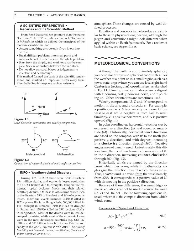
Although the Earth is approximately spherical, you need not always use spherical coordinates. For the weather at a point or in a small region such as a town, state, or province, you can use local right-hand cartesian (rectangular) coordinates, as sketched in Fig. 1.1. Usually, this coordinate system is aligned with x pointing east, y pointing north, and z point-ing up. Other orientations are sometimes used. Velocity components U, V, and W correspond to motion in the x, y, and z directions. For example, a positive value of U is a velocity component from west to east, while negative is from east to west. Similarly, V is positive northward, and W is positive upward (Fig. 1.1). In polar coordinates, horizontal velocities can be expressed as a direction (α), and speed or magni-tude (M). Historically, horizontal wind directions are based on the compass, with 0° to the north (the positive y direction), and with degrees increasing in a clockwise direction through 360°. Negative angles are not usually used. Unfortunately, this dif-fers from the usual mathematical convention of 0° in the x direction, increasing counter-clockwise through 360° (Fig. 1.2). Historically winds are named by the direction from which they come, while in mathematics an-gles give the direction toward which things move. Thus, a west wind is a wind from the west; namely, from 270°. It corresponds to a positive value of U, with air moving in the positive x direction. Because of these differences, the usual trigono-metric equations cannot be used to convert between (U, V) and (α, M). Use the following equations in-stead, where α is the compass direction from which winds come. Conversion to Speed and Direction:

M U V= +( )2 2 1 2/ •(1.1)

α α= −

+90

360°

° ·arctan

CVU o •(1.2a)

a scIentIFIc PersPectIve • descartes and the scientific Method

From René Descartes we get more than the name “Cartesian”. In 1637 he published a book Discours de la Méthode, in which he defined the principles of the modern scientific method:• Accept something as true only if you know it to be true.• Break difficult problems into small parts, and solve each part in order to solve the whole problem.• Start from the simple, and work towards the complex. Seek relationships between the variables.• Do not allow personal biases or judgements to interfere, and be thorough.This method formed the basis of the scientific renais-sance, and marked an important break away from blind belief in philosophers such as Aristotle.

Figure �.�Comparison of meteorological and math angle conventions.

Figure �.�Local Cartesian coordinates and velocity components.

InFo • Weather-related disasters

During 1970 to 2012 there were 8,835 disasters, 1.94 million deaths, and economic losses equivalent to US$ 2.4 trillion due to droughts, temperature ex-tremes, tropical cyclones, floods, and their related health epidemics. Of these totals, storms caused 79% of the disasters, 55% of lives lost, and 86% of economic losses. Individual events included: 300,000 killed in 1970 cyclone Bhola in Bangladesh; 300,000 killed in 1983 drought in Ethiopia; 150,000 killed in drought in Sudan; and 138,866 killed in 1991 cyclone Gorky in Bangladesh. Most of the deaths were in less-de-veloped countries, while most of the economic losses were in the most-developed countries (e.g. US$ 147 billion and $50 billion from hurricanes Katrina and Sandy in the USA). Source: WMO, 2014: “The Atlas of Mortality and Economic Losses from Weather, Climate and Water Extremes, 1970-2012”.

r. stull • practical meteorology �

where αo = 180° if U > 0, but is zero otherwise. C is the angular rotation in a full circle (C = 360° = 2·π radians).

[NOTE: Bullets • identify key equations that are fundamental, or are needed for understanding later chap-ters.]

Some computer languages and spreadsheets al-low a two-argument arc tangent function (atan2):

α = +360180

°atan2 °

CV U· ( , ) (1.2b)

[CAUTION: in the C and C++ programming languages, you might need to switch the order of U & V.]

Some calculators, spreadsheets or computer functions use angles in degrees, while others use radians. If you don’t know which units are used, compute the arccos(–1) as a test. If the answer is 180, then your units are degrees; otherwise, an answer of 3.14159 indicates radians. Use whichever value of C is appropriate for your units.

Conversion to U and V:

U M= − ·sin( )α •(1.3)

V M= − ·cos( )α •(1.4)

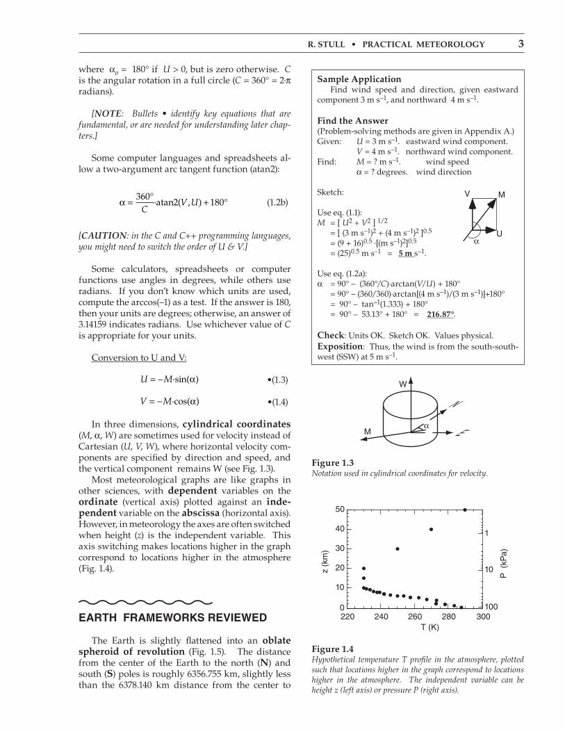
In three dimensions, cylindrical coordinates (M, α, W) are sometimes used for velocity instead of Cartesian (U, V, W), where horizontal velocity com-ponents are specified by direction and speed, and the vertical component remains W (see Fig. 1.3). Most meteorological graphs are like graphs in other sciences, with dependent variables on the ordinate (vertical axis) plotted against an inde-pendent variable on the abscissa (horizontal axis). However, in meteorology the axes are often switched when height (z) is the independent variable. This axis switching makes locations higher in the graph correspond to locations higher in the atmosphere (Fig. 1.4).

earth FraMeWorks revIeWed

The Earth is slightly flattened into an oblate spheroid of revolution (Fig. 1.5). The distance from the center of the Earth to the north (N) and south (s) poles is roughly 6356.755 km, slightly less than the 6378.140 km distance from the center to

sample application Find wind speed and direction, given eastward component 3 m s–1, and northward 4 m s–1.

Find the answer (Problem-solving methods are given in Appendix A.)Given: U = 3 m s–1. eastward wind component. V = 4 m s–1. northward wind component.Find: M = ? m s–1. wind speed α = ? degrees. wind direction

Sketch:

Use eq. (1.1):M = [ U2 + V2 ] 1/2

= [ (3 m s–1)2 + (4 m s–1)2 ]0.5 = (9 + 16)0.5 ·[(m s–1)2]0.5 = (25)0.5 m s–1 = 5 m s–1.

Use eq. (1.2a):α = 90° – (360°/C)·arctan(V/U) + 180° = 90° – (360/360)·arctan[(4 m s–1)/(3 m s–1)]+180° = 90° – tan–1(1.333) + 180° = 90° – 53.13° + 180° = ��6.87°.

check: Units OK. Sketch OK. Values physical.exposition: Thus, the wind is from the south-south-west (SSW) at 5 m s–1.

Figure �.� Notation used in cylindrical coordinates for velocity.

Figure �.4Hypothetical temperature T profile in the atmosphere, plotted such that locations higher in the graph correspond to locations higher in the atmosphere. The independent variable can be height z (left axis) or pressure P (right axis).

4 chapter � • atmospheric Basics

the equator. This 21 km difference in Earth radius causes a north-south cross section (i.e., a slice) of the Earth to be slightly elliptical. But for all practical purposes you can approximate the Earth a sphere (except for understanding Coriolis force in the Forc-es & Winds chapter).

cartography Recall that north-south lines are called merid-ians, and are numbered in degrees longitude. The prime meridian (0° longitude) is defined by inter-national convention to pass through greenwich, Great Britain. We often divide the 360° of longitude around the Earth into halves relative to Greenwich: • Western hemisphere: 0 – 180°W, • eastern hemisphere: 0 – 180°E.

Looking toward the Earth from above the north pole, the Earth rotates counterclockwise about its axis. This means that all objects on the surface of the Earth (except at the poles) move toward the east. East-west lines are called parallels, and are numbered in degrees latitude. By convention, the equator is defined as 0° latitude; the north pole is at 90°N; and the south pole is at 90°S. Between the north and south poles are 180° of latitude, although we usually divide the globe into the: • Northern hemisphere: 0 – 90°N, • southern hemisphere: 0 – 90°S.

On the surface of the Earth, each degree of lati-tude equals 111 km, or 60 nautical miles.

azimuth, Zenith, & elevation angles As a meteorological observer on the ground (black circle in Fig. 1.6), you can describe the local angle to an object (white circle) by two angles: the azimuth angle (α), and either the zenith angle (ζ) or elevation angle (ψ). The object can be physical (e.g., sun, cloud) or an image (e.g., rainbow, sun dog). By “local angle”, we mean angles measured relative to the Cartesian local horizontal plane (e.g., a lake surface, or flat level land surface such as a polder), or relative to the local vertical direction at your loca-tion. Local vertical (up) is defined as opposite to the direction that objects fall. Zenith means “directly overhead”. Zenith angle is the angle measured at your position, between a conceptual line drawn to the zenith (up) and a line drawn to the object (dark arrow in Fig. 1.6). The el-evation angle is how far above the horizon you see the object. Elevation angle and zenith angle are re-lated by: ψ = 90° – ζ , or if your calculator uses radi-ans, it is ψ = π/2 – ζ. Abbreviate both of these forms by ψ = C/4 – ζ, where C = 360° = 2π radians.

sample application A thunderstorm top is at azimuth 225° and eleva-tion angle 60° from your position. How would you describe its location in words? Also, what is the zenith angle?

Find the answer: Given: α = 225° Ψ = 60°. Find: Location in words, and find ζ . (continued next page).

Figure �.6Elevation angle Ψ , zenith angle ζ , and azimuth angle α .

Figure �.5Earth cartography.

r. stull • practical meteorology 5

For the azimuth angle, first project the object vertically onto the ground (A, in Fig. 1.6). Draw a conceptual arrow (dashed) from you to A; this is the projection of the dark arrow on to the local horizon-tal plane. Azimuth angle is the compass angle along the local horizontal plane at your location, measured clockwise from the direction to north (N) to the di-rection to A.

time Zones In the old days each town defined their own lo-cal time. Local noon was when the sun was highest in the sky. In the 1800s when trains and telegraphs allowed fast travel and communication between towns, the railroad companies created standard time zones to allow them to publish and maintain precise schedules. Time zones were eventually ad-opted worldwide by international convention. The Earth makes one complete revolution (rela-tive to the sun) in one day. One revolution contains 360° of longitude, and one day takes 24 hours, thus every hour of elapsed time spans 360°/24 = 15° of longitude. For this reason, each time zone was cre-ated to span 15° of longitude, and almost every zone is 1 hour different from its neighboring time zones. Everywhere within a time zone, all clocks are set to the same time. Sometimes the time-zone boundar-ies are modified to follow political or geographic boundaries, to enhance commerce. coordinated universal time (utc) is the time zone at the prime meridian. It is also known as greenwich mean time (gmt) and Zulu time ( Z ). The prime meridian is in the middle of the UTC time zone; namely, the zone spreads 7.5° on each side of the prime meridian. UTC is the official time used in meteorology, to help coordinate simul-taneous weather observations around the world. Internationally, time zones are given letter desig-nations A - Z, with Z at Greenwich, as already dis-cussed. East of the UTC zone, the local time zones (A, B, C, ...) are ahead; namely, local time of day is later than at Greenwich. West of the UTC zone, the local time zones (N, O, P, ...) are behind; namely, local time of day is earlier than at Greenwich. Each zone might have more than one local name, depending on the countries it spans. Most of west-ern Europe is in the Alpha (A) zone, where A = UTC + 1 hr. This zone is also known as Central Europe Time (CET) or Middle European Time (MET). In N. America are 8 time zones P* - W (see Table 1-1). Near 180° longitude (in the middle of the Pacific Ocean) is the international date line. When you fly from east to west across the date line, you lose a day (it becomes tomorrow). From west to east, you gain a day (it becomes yesterday).

table �-�. Time zones in North America. ST = standard time in the local time zone. DT = daylight time in the local time zone. UTC = coordinated universal time. For conversion, use: ST = UTC – α , DT = UTC – β

Zone Name α (h) β (h)P* Newfoundland 3.5 (NST) 2.5 (NDT)

Q Atlantic 4 (AST) 3 (ADT)

R Eastern 5 (EST) 4 (EDT)

S Central, and Mexico

6 (CST)6 (MEX)

5 (CDT)5

T Mountain 7 (MST) 6 (MDT)

U Pacific 8 (PST) 7 (PDT)

V Alaska 9 (AKST) 8 (AKDT)

W Hawaii-Aleutian

10 (HST) 9 (HDT)

(continuation)Sketch: (see above)Because south has azimuth 180°, and west has azimuth 270°, we find that 225° is exactly halfway between south and west. Hence, the object is southwest (SW) of the observer. Also, 60° elevation is fairly high in the sky. So the thunderstorm top is high in the sky to the southwest of the observer.

Rearrange equation [ Ψ = 90° – ζ ] to solve for zenith angle: ζ = 90° – ψ = 90° - 60° = �0° .

check: Units OK. Locations reasonable. Sketch good.exposition: This is a bad location for a storm chaser (the observer), because thunderstorms in North Amer-ica often move from the SW toward the northeast (NE). Hence, the observer should quickly seek shelter under-ground, or move to a different location out of the storm path.


Many countries utilize Daylight saving time (DT) during their local summer. The purpose is to shift one of the early morning hours of daylight (when people are usually asleep) to the evening (when people are awake and can better utilize the extra daylight). At the start of DT (often in March in North America), you set your clocks one hour ahead. When DT ends in Fall (November), you set your clocks one hour back. The mnemonic “Spring ahead, Fall back” is a useful way to remember. Times can be written as two or four digits. If two, then these digits are hours (e.g., 10 = 10 am, and 14 = 2 pm). If four, then the first two are hours, and the last two are minutes (e.g., 1000 is 10:00 am, and 1435 is 2:35 pm). In both cases, the hours use a 24-h clock going from 0000 (midnight) to 2359 (11:59 pm).

therModynaMIc state

The thermodynamic state of air is measured by its pressure (P), density (ρ), and temperature (T).

temperature When a group of molecules (microscopic) move predominantly in the same direction, the motion is called wind (macroscopic). When they move in random directions, the motion is associated with temperature. Higher temperatures T are associated with greater average molecular speeds v :

T a m vw= · · 2 (1.5)

where a = 4.0x10–5 K·m–2 ·s2 ·mole·g–1 is a con-stant. Molecular weights mw for the most common gases in the atmosphere are listed in Table 1-2. [CAUTION: symbol “a” represents different con-stants for different equations, in this textbook. ]

sample application A weather map is valid at 12 UTC on 5 June. What is the valid local time in Reno, Nevada USA? Hint: Reno is at roughly 120°W longitude.

Find the answer: Given: UTC = 12 , Longitude = 120°W. Find: Local valid time.

First, determine if standard or daylight time: Reno is in the N. Hem., and 5 June is after the start date (March) of DT, so it is daylight time.Hint: each 15° longitude = 1 time zone.Next, use longitude to determine the time zone. 120° / (15° / zone) = 8 zones.But 8 zones difference corresponds to the Pacific Time Zone. (using the ST column of Table 1-1, for which α also indicates the difference in time zones from UTC)Use Table 1-1 for Pacific Daylight Time: β = 7 h PDT = UTC – 7 h = 12 – 7 = 5 am pDt.

check: Units OK. 5 am is earlier than noon.exposition: In the USA, Canada, and Mexico, 12 UTC maps always correspond to morning of the same day, and 00 UTC maps correspond to late afternoon or eve-ning of the previous day.caution: The trick of dividing the longitude by 15° doesn’t work for some towns, where the time zone has been modified to follow geo-political boundaries.

InFo • escape velocity

Fast-moving air molecules that don’t hit other molecules can escape to space by trading their kinetic energy (speed) for potential energy (height). High in the atmosphere where the air is thin, there are few molecules to hit. The lowest escape altitude for Earth is about 550 km above ground, which marks the base of the exosphere (region of escaping gases). This equals 6920 km when measured from the Earth’s cen-ter, and is called the critical radius, rc. The escape velocity, ve , is given by

v

G m

rec

=

2 1 2· · /planet

where G = 6.67x10–11 m3·s–2·kg–1 is the gravitational constant, and mplanet is the mass of the planet. The mass of the Earth is 5.975 x 1024 kg. Thus, the escape velocity from Earth is roughly ve = �0,7�� m s–1. Using this velocity in eq. (1.5) gives the temperature needed for average-speed molecules to escape: 9,222 K for H2, and 18,445 K for the heavier He. Tempera-tures in the exosphere (upper thermosphere) are not hot enough for average-speed H2 and He to escape, but some are faster than average and do escape. Heavier molecules such as O2 have unreachably high escape temperatures (147,562 K), and have stayed in the Earth’s atmosphere, to the benefit of life.

sample application What is the average random velocity of nitrogen molecules at 20°C ?

Find the answer:Given: T = 273.15 + 20 = 293.15 K. Find: v = ? m s–1 (=avg mol. velocity) Sketch: Get mw from Table 1-2. Solve eq. (1.5) for v: v = [T/a·mw]1/2 = [(293.15 K)/(4.0x10–5 K·m–2·s2·mole/g) ·( 28.01g/mole)]1/2 = 5��.5 m s–1 .

check: Units OK. Sketch OK. Physics OK.exposition: Faster than a speeding bullet.

r. stull • practical meteorology 7

Absolute units such as Kelvin (K) must be used for temperature in all thermodynamic and radiative laws. Kelvin is the recommended temperature unit. For everyday use, and for temperature differences, you can use degrees Celsius (°C). [CAUTION: degrees Celsius (°C) and degrees Fahr-enheit (°F) must always be prefixed with the degree symbol (°) to avoid confusion with the electrical units of coulombs (C) and farads (F), but Kelvins (K) never take the degree symbol.] At absolute zero (T = 0 K = –273.15°C) the mol-ecules are essentially not moving. Temperature con-version formulae are:

T TF C° °= +[( / )· ]9 5 32 •(1.6a)

T TC F° °= −( / )·[ ]5 9 32 •(1.6b)

T TK C= +° 273 15. •(1.7a)

T TC K° = − 273 15. •(1.7b)

For temperature differences, you can use ΔT(°C) = ΔT(K), because the size of one degree Celsius is the same as the size of one unit of Kelvin. Hence, only in terms involving temperature differences can you arbitrarily switch between °C and K without need-ing to add or subtract 273.15. Standard (average) sea-level temperature is T = 15.0°C = 288 K = 59°F.Actual temperatures can vary considerably over the course of a day or year. Temperature variation with height is not as simple as the curves for pressure and density, and will be discussed in the Standard At-mosphere section a bit later.

Pressure Pressure P is the force F acting perpendicular (normal) to a surface, per unit surface area A: P F A= / •(1.8)

static pressure (i.e., pressure in calm winds) is caused by randomly moving molecules that bounce off each other and off surfaces they hit. In a vacuum the pressure is zero. In the international system of units (si), a Newton (N) is the unit for force, and m2 is the unit for area. Thus, pressure has units of Newtons per square meter, or N·m–2. One Pascal (Pa) is defined to equal a pressure of 1 N·m–2. The recommended unit for atmospheric pressure is the kilopascal (kpa). The average (standard) pressure at sea level is P = 101.325 kPa. Pressure decreases nearly expo-nentially with height in the atmosphere, below 105 km.

table �-�. Characteristics of gases in the air near the ground. Molecular weights are in g mole–1. The vol-ume fraction indicates the relative contribution to air in the Earth’s lower atmosphere. EPA is the USA Environ-mental Protection Agency.

symbol Name mol.Wt.

VolumeFraction%

constant gases (NASA 2015)

N2O2ArNeHeKrH2Xe

NitrogenOxygenArgonNeonHeliumKryptonHydrogenXenon

28.01 32.00 39.95 20.18 4.00 83.80 2.02131.29

78.0820.950.9340.001 8180.000 5240.000 1140.000 0550.000 009

Variable gasesH2OCO2CH4N2O

Water vaporCarbon dioxideMethaneNitrous oxide

18.0244.0116.0444.01

0 to 40.0400.000170.00003

epa National ambient air Quality standards (NAAQS. 1990 Clean Air Act Amendments. Rules through 2011)

CO

SO2

O3NO2

Carbon monoxide (8 h average) (1 h average)Sulfur dioxide (3 h average) (1 h average)Ozone (8 h average)Nitrogen dioxide (annual average) (1 h average)

28.01

64.06

48.0046.01

0.00090.0035

0.000000050.00000750.0000075

0.00000530.0000100

mean condition for airair 28.96 100.0

table �-�. Standard (average) sea-level pressure.

Value units101.325 kPa 1013.25 hPa 101,325. Pa101,325. N·m–2

101,325 kgm·m–1·s–2

1.033227 kgf·cm–2

1013.25 mb 1.01325 bar14.69595 psi2116.22 psf1.033227 atm760 Torr

kiloPascals (recommended)hectoPascalsPascalsNewtons per square meterkg-mass per meter per s2

kg-force per square cmmillibarsbarspounds-force /square inchpounds-force / square footatmosphereTorr

measured as height of fluid in a barometer:29.92126 in Hg 760 mm Hg33.89854 ft H2O10.33227 m H2O

inches of mercurymillimeters of mercuryfeet of watermeters of water


While kiloPascals will be used in this book, stan-dard sea-level pressure in other units are given in Table 1-3 for reference. Ratios of units can be formed to allow unit conversion (see Appendix A). Although meteorologists are allowed to use hectopascals (as a concession to those meteorologists trained in the previous century, who had grown accustomed to millibars), the prefix “hecto” is non-standard. If you encounter weather maps using millibars or hec-toPascals, you can easily convert to kiloPascals by moving the decimal point one place to the left. In fluids such as the atmosphere, pressure force is isotropic; namely, at any point it pushes with the same force in all directions (see Fig. 1.7a). Similarly, any point on a solid surface experiences pressure forces in all directions from the neighboring fluid elements. At such solid surfaces, all forces cancel ex-cept the forces normal (perpendicular) to the surface (Fig. 1.7b). Atmospheric pressure that you measure at any altitude is caused by the weight of all the air mol-ecules above you. As you travel higher in the at-mosphere there are fewer molecules still above you; hence, pressure decreases with height. Pressure can also compress the air causing higher density (i.e., more molecules in a given space). Compression is greatest where the pressure is greatest, at the bottom of the atmosphere. As a result of more molecules being squeezed into a small space near the bottom than near the top, ambient pressure decreases faster near the ground than at higher altitudes. Pressure change is approximately exponential with height, z. For example, if the temperature (T) were uniform with height (which it is not), then:

P P eoa T z= −· ( / )· (1.9a)

where a = 0.0342 K m–1, and where average sea-level pressure on Earth is Po = 101.325 kPa. For more re-alistic temperatures in the atmosphere, the pressure curve deviates slightly from exponential. This will be discussed in the section on atmospheric struc-ture. [CAUTION again: symbol “a” represents different constants for different equations, in this textbook. ] Equation (1.9a) can be rewritten as:

P P eoz Hp= −

·/ (1.9b)

where Hp = 7.29 km is called the scale height for pressure. Mathematically, Hp is the e-folding dis-tance for the pressure curve.

Figure �.7(a) Pressure is isotropic. (b) Dark vectors correspond to those marked with * in (a). Components parallel to the surface cancel, while those normal to the surface contribute to pressure.

sample application The picture tube of an old TV and the CRT display of an old computer are types of vacuum tube. If there is a perfect vacuum inside the tube, what is the net force pushing against the front surface of a big screen 24 inch (61 cm) display that is at sea level?

Find the answer Given: Picture tube sizes are quantified by the diago-nal length d of the front display surface. Assume the picture tube is square. The length of the side s of the tube is found from: d2 = 2 s2 . The frontal surface area isA = s2 = 0.5 · d2 = 0.5 · (61 cm)2 = 1860.5 cm2

= (1860.5 cm2)·(1 m/100 cm)2 = 0.186 m2 . At sea level, atmospheric pressure pushing against the outside of the tube is 101.325 kPa, while from the inside of the tube there is no force pushing back be-cause of the vacuum. Thus, the pressure difference across the tube face is ΔP = 101.325 kPa = 101.325x103 N m–2.

Find: ΔF = ? N,the net force across the tube.Sketch:

ΔF = Foutside – Finside , but F = P · A. from eq. (1.8) = (Poutside – Pinside )·A = ΔP · A = (101.325x103 N m–2)·( 0.186 m2) = 1.885x104 N = �8.85 kN

check: Units OK. Physically reasonable.exposition: This is quite a large force, and explains why picture tubes are made of such thick heavy glass. For comparison, a person who weighs 68 kg (150 pounds) is pulled by gravity with a force of about 667 N (= 0.667 kN). Thus, the picture tube must be able to support the equivalent of 28 people standing on it!

r. stull • practical meteorology �

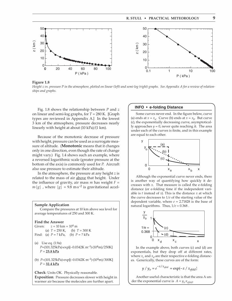
Fig. 1.8 shows the relationship between P and z on linear and semi-log graphs, for T = 280 K. [Graph types are reviewed in Appendix A.] In the lowest 3 km of the atmosphere, pressure decreases nearly linearly with height at about (10 kPa)/(1 km).

Because of the monotonic decrease of pressure with height, pressure can be used as a surrogate mea-sure of altitude. (monotonic means that it changes only in one direction, even though the rate of change might vary.) Fig. 1.4 shows such an example, where a reversed logarithmic scale (greater pressure at the bottom of the axis) is commonly used for P. Aircraft also use pressure to estimate their altitude. In the atmosphere, the pressure at any height z is related to the mass of air above that height. Under the influence of gravity, air mass m has weight F = m·|g| , where |g| = 9.8 m·s–2 is gravitational accel-

InFo • e-folding distance

Some curves never end. In the figure below, curve (a) ends at x = xa. Curve (b) ends at x = xb. But curve (c), the exponentially decreasing curve, asymptotical-ly approaches y = 0, never quite reaching it. The area under each of the curves is finite, and in this example are equal to each other.

Although the exponential curve never ends, there is another way of quantifying how quickly it de-creases with x. That measure is called the e-folding distance (or e-folding time if the independent vari-able is t instead of x). This is the distance x at which the curve decreases to 1/e of the starting value of the dependent variable, where e = 2.71828 is the base of natural logarithms. Thus, 1/e = 0.368 .

In the example above, both curves (c) and (d) are exponentials, but they drop off at different rates, where xc and xd are their respective e-folding distanc-es. Generically, these curves are of the form:

y y e x xox x

efoldefold/ exp( / )

/= = −−

Another useful characteristic is that the area A un-der the exponential curve is A = yo·xefold.

sample application Compare the pressures at 10 km above sea level for average temperatures of 250 and 300 K.

Find the answer Given: z = 10 km = 104 m (a) T = 250 K, (b) T = 300 KFind: (a) P = ? kPa, (b) P = ? kPa

(a) Use eq. (1.9a): P=(101.325kPa)·exp[(–0.0342K m–1)·(104m)/250K] P = �5.8 kpa

(b) P=(101.325kPa)·exp[(–0.0342K m–1)·(104m)/300K] P = ��.4 kpa

check: Units OK. Physically reasonable.exposition: Pressure decreases slower with height in warmer air because the molecules are further apart.

Figure �.8 Height z vs. pressure P in the atmosphere, plotted on linear (left) and semi-log (right) graphs. See Appendix A for a review of relation-ships and graphs.

�0 chapter � • atmospheric Basics

eration at the Earth’s surface. This weight is a force that squeezes air molecules closer together, increas-ing both the density and the pressure. Knowing that P = F/A, previous two expressions are combined to give

Pz = |g|·mabove z / A (1.10)

where A is horizontal cross-section area. Similarly, between two different pressure levels is mass

∆m = (A/|g|)·(Pbottom – Ptop) (1.11)

density Density ρ is defined as mass m per unit volume Vol.

ρ = m Vol/ •(1.12)

Density increases as the number and molecular weight of molecules in a volume increase. Average air density at sea level is given in Table 1-4. The rec-ommended unit for density is kg·m–3 . Because gases such as air are compressible, air density can vary over a wide range. Density de-creases roughly exponentially with height in an at-mosphere of uniform temperature.

ρ ρ= −o

a T ze· ( / )· (1.13a)or ρ ρ ρ= −

oz He· / (1.13b)

where a = 0.040 K m–1, and where average sea-level density is ρo = 1.2250 kg·m–3, at a temperature of 15°C = 288 K. The shape of the curve described by eq. (1.13) is similar to that for pressure, (see Fig. 1.9). The scale height for density is Hρ = 8.55 km. Although the air is quite thin at high altitudes, it still can affect many observable phenomena: twi-light (scattering of sunlight by air molecules) up to

table �-4. Standard atmospheric density at sea lev-el, for a standard temperature 15°C.

Value units1.2250 kg·m–3.

0.076474 lbm ft–3

1.2250 g liter–1

0.001225 g cm–3

kilograms per cubic meter (recommended)pounds-mass per cubic footgrams per litergrams per cubic centimeter

sample application At sea level, what is the mass of air within a room of size 5 m x 8 m x 2.5 m ?

Find the answer Given: L = 8 m room length, W = 5 m width H = 2.5 m height of room ρ = 1.225 kg·m-3 at sea levelFind: m = ? kg air mass

The volume of the room is Vol = W·L·H = (5m)·(8m)·(2.5m) = 100 m3. Rearrange eq. (1.12) and solve for the mass: m = ρ·Vol. = (1.225 kg·m-3)·(100 m3) = ��.5 kg.

check: Units OK. Sketch OK. Physics OK.exposition: This is 1.5 to 2 times a person’s mass.

sample application What is the air density at a height of 2 km in an atmosphere of uniform temperature of 15°C?

Find the answer Given: z =2000 m, ρo =1.225 kg m–3 , T =15°C =288.15 KFind: ρ = ? kg m–3

Use eq. (1.13): ρ=(1.225 kg m–3)· exp[(–0.04 K m–1)·(2000 m)/288 K] ρ = 0.��8 kg m–3

check: Units OK. Physics reasonable.exposition: This means that aircraft wings generate 24% less lift, and engines generate 24% less thrust be-cause of the reduced air density.

Figure �.�Density ρ vs. height z in the atmosphere.

sample application Over each square meter of Earth’s surface, how much air mass is between 80 and 30 kPa?

Find the answer:Given: Pbottom = 80 kPa, Ptop = 30 kPa, A = 1 m2 Find: ∆m = ? kg

Use eq. (1.11): ∆m = [(1 m2)/(9.8 ms–2)]·(80 – 30 kPa)· [(1000 kg·m–1·s–2 )/(1 kPa)] = 5�0� kg check: Units OK. Physics OK. Magnitude OK.exposition: About 3 times the mass of a car.

r. stull • practical meteorology ��

63 km, meteors (incandescence by friction against air molecules) from 110 to 200 km, and aurora (exci-tation of air by solar wind) from 360 to 500 km. The specific volume (α) is defined as the inverse of density (α = 1/ρ). It has units of volume/mass.

atMosPherIc structure

Atmospheric structure refers to the state of the air at different heights. The true vertical structure of the atmosphere varies with time and location due to changing weather conditions and solar activity.

standard atmosphere The “1976 U.S. Standard Atmosphere” (Table 1-5) is an idealized, dry, steady-state approximation of atmospheric state as a function of height. It has been adopted as an engineering reference. It approxi-mates the average atmospheric conditions, although it was not computed as a true average. A geopotential height, H, is defined to com-pensate for the decrease of gravitational acceleration magnitude |g| above the Earth’s surface:

H R z R zo o= +· /( ) •(1.14a)

z R H R Ho o= −· /( ) •(1.14b)

where the average radius of the Earth is Ro = 6356.766 km. An air parcel (a group of air molecules mov-ing together) raised to geometric height z would have the same potential energy as if lifted only to height H under constant gravitational acceleration. By using H instead of z, you can use |g| = 9.8 m s–2 as a constant in your equations, even though in real-ity it decreases slightly with altitude. The difference (z – H) between geometric and geopotential height increases from 0 to 16 m as height increases from 0 to 10 km above sea level. Sometimes g and H are combined into a new variable called the geopotential, Φ:

Φ = g H· (1.15)

Geopotential is defined as the work done against gravity to lift 1 kg of mass from sea level up to height H. It has units of m2 s–2.

hIgher Math • geopotential height

What is “higher math”? These boxes contain supplementary material that use calculus, differential equations, linear algebra, or other mathematical tools beyond algebra. They are not essential for understanding the rest of the book, and may be skipped. Science and engineering stu-dents with calculus backgrounds might be curious about how calculus is used in atmospheric physics.

geopotential height For gravitational acceleration magnitude, let |go| = 9.8 m s–2 be average value at sea level, and |g| be the value at height z. If Ro is Earth radius, then r = Ro + z is distance above the center of the Earth. Newton’s Gravitation Law gives the force |F| be-tween the Earth and an air parcel:

|F| = G · mEarth · mair parcel / r2 where G = 6.67x10–11 m3·s–2·kg–1 is the gravitational constant. Divide both sides by mair parcel, and recall that by definition |g| = |F|/mair parcel. Thus

|g| = G · mEarth / r2

This eq. also applies at sea level (z = 0):

|go| = G · mEarth/ Ro2

Combining these two eqs. give

|g| = |go| · [ Ro / (Ro + z) ]2

Geopotential height H is defined as the work per unit mass to lift an object against the pull of gravity, divided by the gravitational acceleration value for sea level:

Hg

g dZo Z

z

==∫1

0

·

Plugging in the definition of |g| from the previous paragraph gives:

H R R Z dZo oZ

z

= +( )−

=∫2 2

0

·

This integrates to

HR

R Zo

o Z

z

=−

+=

2

0

After plugging in the limits of integration, and put-ting the two terms over a common denominator, the answer is: H R z R zo o= +· /( ) (1.14a)

�� chapter � • atmospheric Basics

Table 1-5 gives the standard temperature, pres-sure, and density as a function of geopotential height H above sea level. Temperature variations are linear between key altitudes indicated in boldface. Stan-dard-atmosphere temperature is plotted in Fig. 1.10. Below a geopotential altitude of 51 km, eqs. (1.16) and (1.17) can be used to compute standard tempera-ture and pressure. In these equations, be sure to use absolute temperature as defined by T(K) = T(°C) + 273.15 . (1.16)

T = 288.15 K – (6.5 K km–1)·H for H ≤ 11 km

T = 216.65 K 11 ≤ H ≤ 20 km

T = 216.65 K +(1 K km–1)·(H–20km) 20 ≤ H ≤ 32 km

T = 228.65 K +(2.8 K km–1)·(H–32km) 32 ≤ H ≤ 47 km

T = 270.65 K 47 ≤ H ≤ 51 km

For the pressure equations, the absolute tempera-ture T that appears must be the standard atmosphere temperature from the previous set of equations. In fact, those previous equations can be substituted into the equations below to make them a function of H rather than T. (1.17)

P = (101.325kPa)·(288.15K/T) –5.255877 H ≤ 11 km

P = (22.632kPa)·exp[–0.1577·(H–11 km)] 11 ≤ H ≤ 20 km

table �-5. Standard atmosphere.

h (km) t (°c) p (kpa) ρ (kg m–�)-1012345678910��131517�02530��35404547505�60707�80

84.�89.7

100.4105110

21.515.08.52.0-4.5-11.0-17.5-24.0-30.5-37.0-43.5-50.0-56.5-56.5-56.5-56.5-56.5-51.5-46.5-44.5-36.1-22.1-8.1-2.5-2.5-2.5-27.7-55.7-58.5-76.5-86.3-86.3-73.6-55.5-9.2

113.920101.32589.87479.49570.10861.64054.01947.18141.06035.59930.74226.43622.63216.51012.0448.7875.4752.5111.1720.8680.5590.2780.1430.1110.0760.067

0.020310.004630.003960.000890.000370.000150.000020.000010.00001

1.34701.22501.11161.00650.90910.81910.73610.65970.58950.52520.46640.41270.36390.26550.19370.14230.08800.03950.01800.01320.00820.00390.00190.00140.0010

0.000860.0002880.0000740.0000640.0000150.0000070.000003

0.00000050.00000020.0000001

sample application Find the geopotential height and the geopotential at 12 km above sea level.

Find the answerGiven: z = 12 km, Ro = 6356.766 kmFind: H = ? km, Φ = ? m2 s–2

Use eq. (1.14a): H = (6356.766km)·(12km) / ( 6356.766km + 12km ) = ��.�8 km Use eq. (1.15): Φ = (9.8 m s–2)·(11,980 m) =�.�7x�05 m2 s–2 check: Units OK. exposition: H ≤ z as expected, because you don’t need to lift the parcel as high for constant gravity as you would for decreasing gravity, to do the same work.

sample application Find std. atm. temperature & pressure at H=2.5 km.

Find the answerGiven: H = 2.5 km. Find: T = ? K, P = ? kPaUse eq. (1.16): T = 288.15 –(6.5K/km)·(2.5km) = �7�.� KUse eq. (1.17): P =(101.325kPa)·(288.15K/271.9K)–5.255877 = (101.325kPa)· 0.737 = 74.7 kpa. check: T = –1.1°C. Agrees with Fig. 1.10 & Table 1-5.

Figure �.�0Standard temperature T profile vs. geopotential height H.


P = (5.4749kPa)·(216.65K/T) 34.16319 20 ≤ H ≤ 32 km

P = (0.868kPa)·(228.65K/T) 12.2011 32 ≤ H ≤ 47 km

P = (0.1109kPa)·exp[–0.1262·(H–47 km)] 47 ≤ H ≤ 51 km

These equations are a bit better than eq. (1.9a) be-cause they do not make the unrealistic assumption of uniform temperature with height. Knowing temperature and pressure, you can cal-culate density using the ideal gas law eq. (1.18).

layers of the atmosphere The following layers are defined based on the nominal standard-atmosphere temperature struc-ture (Fig. 1.10).

thermosphere 84.9 ≤ H km mesosphere 47 ≤ H ≤ 84.9 km stratosphere 11 ≤ H ≤ 47 km troposphere 0 ≤ H ≤ 11 km

Almost all clouds and weather occur in the tropo-sphere. The top limits of the bottom three spheres are named:

mesopause H = 84.9 km stratopause H = 47 km tropopause H = 11 km

On average, the tropopause is lower (order of 8 km) near the Earth’s poles, and higher (order of 18 km) near the equator. In mid-latitudes, the tropopause height averages about 11 km, but is slightly lower in winter, and higher in summer. The three relative maxima of temperature are a result of three altitudes where significant amounts of solar radiation are absorbed and converted into heat. Ultraviolet light is absorbed by ozone near the stratopause, visible light is absorbed at the ground, and most other radiation is absorbed in the thermo-sphere.

atmospheric Boundary layer The bottom 0.3 to 3 km of the troposphere is called the atmospheric boundary layer (aBl). It is often turbulent, and varies in thickness in space and time (Fig. 1.11). It “feels” the effects of the Earth’s surface, which slows the wind due to surface drag, warms the air during daytime and cools it at night, and changes in moisture and pollutant concentra-tion. We spend most of our lives in the ABL. Details are discussed in a later chapter.

sample application Is eq. (1.9a) a good fit to standard atmos. pressure?

Find the answerAssumption: Use T = 270 K in eq. (1.9a) because it min-imizes pressure errors in the bottom 10 km.Method: Compare on a graph where the solid line is eq. (1.9a) and the data points are from Table 1-5.

exposition: Over the lower 10 km, the simple eq. (1.9a) is in error by no more than 1.5 kPa. If more ac-curacy is needed, then use the hypsometric equation (see eq. 1.26, later in this chapter).

Figure �.��Boundary layer (shaded) within the bottom of the troposphere. Standard atmosphere is dotted. Typical temperature profiles during day (black line) and night (grey line) Boundary-layer top (dashed line) is at height zi.


equatIon oF state– Ideal gas laW

Because pressure is caused by the movement of molecules, you might expect the pressure P to be greater where there are more molecules (i.e., greater density ρ), and where they are moving faster (i.e., greater temperature T). The relationship between pressure, density, and temperature is called the equation of state. Different fluids have different equations of state, depending on their molecular properties. The gas-es in the atmosphere have a simple equation of state known as the ideal gas law. For dry air (namely, air with the usual mix of gases, except no water vapor), the ideal gas law is:

P Td= ℜρ· · •(1.18)

where ℜd = 0.287053 kPa·K–1·m3·kg–1

= 287.053 J·K–1·kg–1 .

ℜd is called the gas constant for dry air. Absolute temperatures (K) must be used in the ideal gas law. The total air pressure P is the sum of the partial pressures of nitrogen, oxygen, water vapor, and the other gases. A similar equation of state can be written for just the water vapor in air:

e Tv v= ℜρ · · (1.19)

where e is the partial pressure due to water vapor (called the vapor pressure), ρv is the density of wa-ter vapor (called the absolute humidity), and the gas constant for pure water vapor is

ℜv = 0.4615 kPa·K–1·m3·kg–1

= 461.5 J·K–1·kg–1 . For moist air (normal gases with some water va-por),

P T= ℜρ· · (1.20)

where density ρ is now the total density of the air. A difficulty with this last equation is that the “gas constant” is NOT constant. It changes as the humid-ity changes because water vapor has different mo-lecular properties than dry air. To simplify things, a virtual temperature Tv can be defined to include the effects of water vapor:

T T a rv = +·[ ( · )]1 •(1.21)

sample application In an unsaturated tropical environment with tem-perature of 35°C and water-vapor mixing ratio of 30 gwater vapor/kgdry air, what is the virtual temperature?

Find the answer:Given: T = 35°C, r = 30 gwater vapor/kgdry airFind: Tv = ? °C

First, convert T and r to proper units T = 273.15 + 35 = 308.15 K.r =(30 gwater/kg air)·(0.001 kg/g) = 0.03 gwater/g air

Next use eq. (1.21): Tv = (308.15 K)·[ 1 + (0.61 · 0.03) ] = 313.6 K = 40.6°c.

check: Units OK. Physically reasonable.exposition: Thus, high humidity reduces the density of the air so much that it acts like dry air that is 5°C warmer, for this case.

sample application What is the absolute humidity of air of temperature 20°C and water vapor pressure of 2 kPa?

Find the answer: Given: e = 2 kPa, T = 20°C = 293 K Find: ρv = ? kgwater vapor ·m-3

Solving eq. (1.19) for ρv gives: ρv = e / (ℜv·T) ρv = ( 2 kPa ) / ( 0.4615 kPa·K–1·m3·kg–1 · 293 K ) = 0.0�48 kgwater vapor ·m-3

check: Units OK. Physically reasonable.exposition: Small compared to the total air density.

sample application What is the average (standard) surface temperature for dry air, given standard pressure and density?

Find the answer: Given: P = 101.325 kPa, ρ = 1.225 kg·m-3

Find: T = ? K

Solving eq. (1.18) for T gives: T = P / (ρ·ℜd)

T = 101 325

1 225 0 287

.

( . )·( .

kPa

kg·m kPa·K ·-3 -1 mm ·kg3 -1)

= 288.2 K = �5°c

check: Units OK. Physically reasonable.exposition: The answer agrees with the standard surface temperature of 15°C discussed earlier, a cool but pleasant temperature.

r. stull • practical meteorology �5

where r is the water-vapor mixing ratio [r = (mass of water vapor)/(mass of dry air), with units gwater vapor /gdry air, see the Water Vapor chapter], a = 0.61 gdry air/gwater vapor, and all temperatures are in absolute units (K). In a nutshell, moist air of tem-perature T behaves as dry air with temperature Tv . Tv is greater than T because water vapor is less dense than dry air, and thus moist air acts like warmer dry air. If there is also liquid water or ice in the air, then this virtual temperature must be modified to in-clude the liquid-water loading (i.e., the weight of the drops falling at their terminal velocity) and ice loading:

T T a r r rv L I= + − −·[ ( · ) ]1 •(1.22)

where rL is the liquid-water mixing ratio (gliquid wa-ter / gdry air), rI is the ice mixing ratio (gice / gdry air), and a = 0.61 (gdry air / g water vapor ). Because liquid water and ice are heavy, air with liquid-water and/or ice loading acts like colder dry air. With these definitions, a more useful form of the ideal gas law can be written for air of any humid-ity: P Td v= ℜρ· · •(1.23)

where ℜd is still the gas constant for dry air. In this form of the ideal gas law, the effects of variable hu-midity are hidden in the virtual temperature factor, which allows the dry “gas constant” to be used (nice, because it really is constant).

hydrostatIc equIlIBrIuM

As discussed before, pressure decreases with height. Any thin horizontal slice from a column of air would thus have greater pressure pushing up against the bottom than pushing down from the top (Fig. 1.12). This is called a vertical pressure gradi-ent, where the term gradient means change with distance. The net upward force acting on this slice of air, caused by the pressure gradient, is F = ΔP·A, where A is the horizontal cross section area of the column, and ΔP = Pbottom – Ptop. Also acting on this slice of air is gravity, which provides a downward force (weight) given by

F m g= · •(1.24)

where g = – 9.8 m·s–2 is the gravitational accelera-tion. (See Appendix B for variation of g with lati-tude and altitude.) Negative g implies a negative

sample application In a tropical environment with temperature of 35°C, water-vapor mixing ratio of 30 gwater vapor/kgdry

air , and 10 gliquid water/kgdry air of raindrops falling at their terminal velocity through the air, what is the virtual temperature?

Find the answer:Given: T = 35°C, r = 30 gwater vapor/kgdry air rL = 10 gliquid water/kgdry air Find: Tv = ? °C

First, convert T , r and rL to proper units T = 273.15 + 35 = 308.15 K.r =(30 gvapor/kg air)·(0.001 kg/g) = 0.03 gvapor/g airrL =(10 gliquid/kg air)·(0.001 kg/g) = 0.01 gliquid/g air

Next use eq. (1.22): Tv = (308.15 K)·[ 1 + (0.61 · 0.03) – 0.01 ] = 310.7 K = �7.6°c.

check: Units OK. Physically reasonable.exposition: Compared to the previous Sample Ap-plication, the additional weight due to falling rain made the air act like it was about 3°C cooler.

Figure �.��.Hydrostatic balance of forces on a thin slice of air.

sample application What is the weight (force) of a person of mass 75 kg at the surface of the Earth?

Find the answerGiven: m = 75 kgFind: F = ? N

Sketch: Use eq. (1.24) F = m·g = (75 kg)·(– 9.8 m·s–2) = – 735 kg·m·s–2 = – 7�5 N

check: Units OK. Sketch OK. Physics OK.exposition: The negative sign means the person is pulled toward the Earth, not repelled away from it.


(downward) force. (Remember that the unit of force is 1 N = 1 kg·m·s–2 , see Appendix A). The mass m of air in the slice equals the air density times the slice volume; namely, m = ρ · (A·Δz), where Δz is the slice thickness. For situations where pressure gradient force ap-proximately balances gravity force, the air is said to be in a state of hydrostatic equilibrium. The cor-responding hydrostatic equation is:

∆ ∆P g z= ρ· · (1.25a)

or

∆∆Pz

g= – ·ρ •(1.25b)

The term hydrostatic is used because it de-scribes a stationary (static) balance in a fluid (hydro) between pressure pushing up and gravity pulling down. The negative sign indicates that pressure decreases as height increases. This equilibrium is valid for most weather situations, except for vigor-ous storms with large vertical velocities.

hIgher Math • Physical Interpretation of equations

Equations such as (1.25b) are finite-difference ap-proximations to the original equations that are in dif-ferential form: d

d– ·

Pz

g= ρ (1.25c)

The calculus form (eq. 1.25c) is useful for derivations, and is the best description of the physics. The alge-braic approximation eq. (1.25b) is often used in real life, where one can measure pressure at two different heights [i.e., ΔP/Δz = (P2 – P1)/ (z2 – z1)]. The left side of eq. (1.25c) describes the infinitesi-mal change of pressure P that is associated with an infinitesimal local change of height z. It is the vertical gradient of pressure. On a graph of P vs. z, it would be the slope of the line. The derivative symbol “d” has no units or dimensions, so the dimensions of the left side are kPa m–1. Eq. (1.25b) has a similar physical interpretation. Namely, the left side is the change in pressure associ-ated with a finite change in height. Again, it repre-sents the slope of a line, but in this case, it is a straight line segment of finite length, as an approximation to a smooth curve. Both eqs. (1.25b & c) state that rate of pressure de-crease (because of the negative sign) with height is greater if the density ρ is greater, or if the magnitude of the gravitational acceleration |g| is greater. Name-ly, if factors ρ or |g| increase, then the whole right hand side (RHS) increases because ρ and |g| are in the numerator. Also, if the RHS increases, then the left hand side (LHS) must increase as well, to preserve the equality of LHS = RHS.

sample application Near sea level, a height increase of 100 m corre-sponds to what pressure decrease?

Find the answerGiven: ρ= 1.225 kg·m–3 at sea level Δz = 100 mFind: ΔP = ? kPaSketch:

Use eq. (1.25a):ΔP = ρ·g·Δz = ( 1.225 kg·m–3)·(–9.8 m·s–2)·(100 m) = – 1200.5 kg·m–1·s–2

= – �.�0 kpa

check: Units OK. Sketch OK. Physics OK.exposition: This answer should not be extrapolated to greater heights.

a scIentIFIc PersPectIve • check for errors

As a scientist or engineer you should always be very careful when you do your calculations and de-signs. Be precise. Check and double check your calculations and your units. Don’t take shortcuts, or make unjustifiable simplifications. Mistakes you make as a scientist or engineer can kill people and cause great financial loss. Be careful whenever you encounter any equa-tion that gives the change in one variable as a func-tion of change of another. For example, in equa-tions (1.25) P is changing with z. The “change of” operator (Δ) MUST be taken in the same direction for both variables. In this example ΔP/Δz means [ P(at z2) – P(at z1) ] / [ z2 – z1 ] . We often abbreviate this as [ P2 – P1 ] / [ z2 – z1 ]. If you change the denominator to be [ z1 – z2 ], then you must also change the numerator to be in the same direction [ P1 – P2 ] . It doesn’t matter which direction you use, so long as both the numerator and denominator (or both Δ variables as in eq. 1.25a) are in the same direction. To help avoid errors in direction, you should al-ways think of the subscripts by their relative posi-tions in space or time. For example, subscripts 2 and 1 often mean top and bottom, or right and left, or later and earlier, etc. If you are not careful, then when you solve numerical problems using equations, your an-swer will have the wrong sign, which is sometimes difficult to catch.


hyPsoMetrIc equatIon

When the ideal gas law and the hydrostatic equa-tion are combined, the result is an equation called the hypsometric equation. This allows you to calculate how pressure varies with height in an at-mosphere of arbitrary temperature profile:

z z a TPPv2 1

1

2− ≈

· ·ln •(1.26a)

or

P Pz z

a Tv2 1

1 2= −

·exp·

•(1.26b)

where Tv is the average virtual temperature be-tween heights z1 and z2. The constant a = ℜd /|g| = 29.3 m K–1. The height difference of a layer bounded below and above by two pressure levels P1 (at z1) and P2 (at z2) is called the thickness of that layer. To use this equation across large height differ-ences, it is best to break the total distance into a number of thinner intervals, Δz. In each thin layer, if the virtual temperature varies little, then you can approximate by Tv. By this method you can sum all of the thicknesses of the thin layers to get the total thickness of the whole layer. For the special case of a dry atmosphere of uni-form temperature with height, eq. (1.26b) simplifies to eq. (1.9a). Thus, eq. (1.26b) also describes an expo-nential decrease of pressure with height.

Process terMInology

Processes associated with constant temperature are isothermal. For example, eqs. (1.9a) and (1.13a) apply for an isothermal atmosphere. Those occur-ring with constant pressure are isobaric. A line on a weather map connecting points of equal tem-perature is called an isotherm, while one connect-ing points of equal pressure is an isobar. Table 1-6 summarizes many of the process terms.

sample application (§) What is the thickness of the 100 to 90 kPa layer, given [P(kPa), T(K)] = [90, 275] and [100, 285].

Find the answerGiven: observations at top and bottom of the layerFind: Δz = z2 – z1Assume: T varies linearly with z. Dry air: T = Tv.

Solve eq. (1.26) on a computer spreadsheet (§) for many thin layers 0.5 kPa thick. Results for the first few thin layers, starting from the bottom, are:

P(kPa) Tv (K) Tv (K) Δz(m)

10099.599.0

285284.5284

284.75284.25etc.

41.8241.96etc.

Sum of all Δz = 864.�� m

check: Units OK. Physics reasonable.exposition: In an aircraft you must climb 864.11 m to experience a pressure decrease from 100 to 90 kPa, for this particular temperature sounding. If you com-pute the whole thickness at once from ∆z = (29.3m K–1)·(280K)·ln(100/90) = 864.38 m, this answer is less accurate than by summing over smaller thicknesses.

table �-6.Process names. (tendency = change with time)

Name constant or equaladiabatcontourisallobarisallohypseisallothermisanabatisanomalisentropeisobarisobathisobathythermisoceraunicisochroneisodopisodrosothermisoechoisogonisogramisohelisohumeisohyetisohypseisolineisonephisoplethisopycnicisoshearisostereisotachisotherm

entropy (no heat exchange)heightpressure tendencyheight tendencytemperature tendencyvertical wind speedweather anomalyentropy or potential temp.pressurewater depthdepth of constant temperaturethunderstorm activity or freq.time(Doppler) radial wind speeddew-point temperatureradar reflectivity intensitywind direction(generic, for any quantity)sunshinehumidityprecipitation accumulationheight (similar to contour)(generic, for any quantity)cloudiness(generic, for any quantity)densitywind shearspecific volume (1/ρ)speedtemperature

sample application Name the process for constant density.

Find the answer: From Table 1-6: It is an isopycnal process.

exposition: Isopycnics are used in oceanography, where both temperature and salinity affect density.


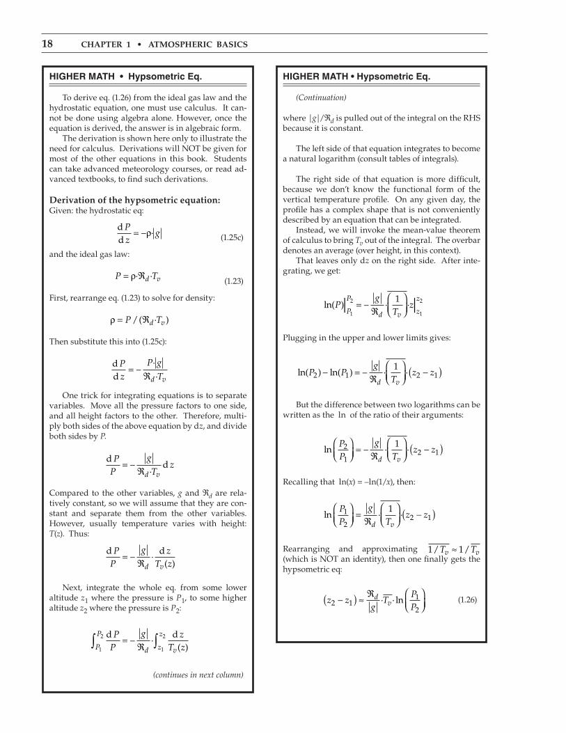
hIgher Math • hypsometric eq.

(Continuation)

where |g|/ℜd is pulled out of the integral on the RHS because it is constant.

The left side of that equation integrates to become a natural logarithm (consult tables of integrals).

The right side of that equation is more difficult, because we don’t know the functional form of the vertical temperature profile. On any given day, the profile has a complex shape that is not conveniently described by an equation that can be integrated. Instead, we will invoke the mean-value theorem of calculus to bring Tv out of the integral. The overbar denotes an average (over height, in this context). That leaves only dz on the right side. After inte-grating, we get:

ln( ) –| |P

g

Tz

P

P

d v z

z

1

2

1

21=ℜ

· ·

Plugging in the upper and lower limits gives:

ln( ) ln( ) –P Pg

Tz z

d v2 1 2 1

1− =ℜ

−( )· ·

But the difference between two logarithms can be written as the ln of the ratio of their arguments:

ln –PP

g

Tz z

d v

2

12 1

1

=ℜ

−( )· ·

Recalling that ln(x) = –ln(1/x), then:

ln ·PP

g

Tz z

d v

1

22 1

1

=ℜ

−( )·

Rearranging and approximating 1 1/ /T Tv v≈ (which is NOT an identity), then one finally gets the hypsometric eq:

z zg

TPP

dv2 1

1

2−( ) ≈

ℜ

· · ln (1.26)

hIgher Math • hypsometric eq.

To derive eq. (1.26) from the ideal gas law and the hydrostatic equation, one must use calculus. It can-not be done using algebra alone. However, once the equation is derived, the answer is in algebraic form. The derivation is shown here only to illustrate the need for calculus. Derivations will NOT be given for most of the other equations in this book. Students can take advanced meteorology courses, or read ad-vanced textbooks, to find such derivations.

Derivation of the hypsometric equation:Given: the hydrostatic eq:

dd

– ·Pz

g= ρ (1.25c)

and the ideal gas law:

P Td v= ℜρ· · (1.23)

First, rearrange eq. (1.23) to solve for density:

ρ = ℜP Td v/( · )

Then substitute this into (1.25c):

dd

–··

Pz

P g

Td v=

ℜ

One trick for integrating equations is to separate variables. Move all the pressure factors to one side, and all height factors to the other. Therefore, multi-ply both sides of the above equation by dz, and divide both sides by P.

d

–·

dP

P

g

Tz

d v=

ℜ

Compared to the other variables, g and ℜd are rela-tively constant, so we will assume that they are con-stant and separate them from the other variables. However, usually temperature varies with height: T(z). Thus:

d

–d

( )P

P

g zT zd v

=ℜ

·

Next, integrate the whole eq. from some lower altitude z1 where the pressure is P1, to some higher altitude z2 where the pressure is P2:

d

–d

( )P

P

g zT zP

P

d vz

z

1

2

1

2∫ ∫=ℜ

·

(continues in next column)


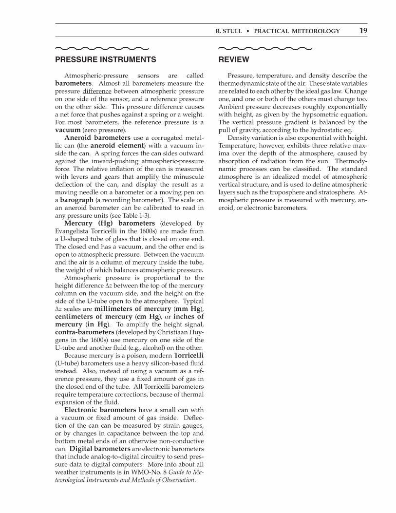
Pressure InstruMents

Atmospheric-pressure sensors are called barometers. Almost all barometers measure the pressure difference between atmospheric pressure on one side of the sensor, and a reference pressure on the other side. This pressure difference causes a net force that pushes against a spring or a weight. For most barometers, the reference pressure is a vacuum (zero pressure). aneroid barometers use a corrugated metal-lic can (the aneroid element) with a vacuum in-side the can. A spring forces the can sides outward against the inward-pushing atmospheric-pressure force. The relative inflation of the can is measured with levers and gears that amplify the minuscule deflection of the can, and display the result as a moving needle on a barometer or a moving pen on a barograph (a recording barometer). The scale on an aneroid barometer can be calibrated to read in any pressure units (see Table 1-3). mercury (hg) barometers (developed by Evangelista Torricelli in the 1600s) are made from a U-shaped tube of glass that is closed on one end. The closed end has a vacuum, and the other end is open to atmospheric pressure. Between the vacuum and the air is a column of mercury inside the tube, the weight of which balances atmospheric pressure. Atmospheric pressure is proportional to the height difference ∆z between the top of the mercury column on the vacuum side, and the height on the side of the U-tube open to the atmosphere. Typical ∆z scales are millimeters of mercury (mm hg), centimeters of mercury (cm hg), or inches of mercury (in hg). To amplify the height signal, contra-barometers (developed by Christiaan Huy-gens in the 1600s) use mercury on one side of the U-tube and another fluid (e.g., alcohol) on the other. Because mercury is a poison, modern torricelli (U-tube) barometers use a heavy silicon-based fluid instead. Also, instead of using a vacuum as a ref-erence pressure, they use a fixed amount of gas in the closed end of the tube. All Torricelli barometers require temperature corrections, because of thermal expansion of the fluid. electronic barometers have a small can with a vacuum or fixed amount of gas inside. Deflec-tion of the can can be measured by strain gauges, or by changes in capacitance between the top and bottom metal ends of an otherwise non-conductive can. Digital barometers are electronic barometers that include analog-to-digital circuitry to send pres-sure data to digital computers. More info about all weather instruments is in WMO-No. 8 Guide to Me-teorological Instruments and Methods of Observation.

revIeW

Pressure, temperature, and density describe the thermodynamic state of the air. These state variables are related to each other by the ideal gas law. Change one, and one or both of the others must change too. Ambient pressure decreases roughly exponentially with height, as given by the hypsometric equation. The vertical pressure gradient is balanced by the pull of gravity, according to the hydrostatic eq. Density variation is also exponential with height. Temperature, however, exhibits three relative max-ima over the depth of the atmosphere, caused by absorption of radiation from the sun. Thermody-namic processes can be classified. The standard atmosphere is an idealized model of atmospheric vertical structure, and is used to define atmospheric layers such as the troposphere and stratosphere. At-mospheric pressure is measured with mercury, an-eroid, or electronic barometers.


tips At the end of each chapter are four types of homework exercises: • Broaden Knowledge & Comprehension • Apply • Evaluate & Analyze • SynthesizeEach of these types are explained here in Chapter 1, at the start of their respective subsections. I also recommend how you might approach these differ-ent types of problems. One of the first tips is in the “A SCIENTIFIC PER-SPECTIVE” box. Here I recommend that you write your exercise solutions in a format very similar to the “Solved Examples” that I have throughout this book. Such meticulousness will help you earn high-er grades in most science and engineering courses, and will often give you partial credit (instead of zero credit) for exercises you solved incorrectly. Finally, most of the exercises have multiple parts to them. Your instructor need assign only one of the parts for you to gain the skills associated with that exercise. Many of the numerical problems are similar to Solved Examples presented earlier in the chapter. Thus, you can try to do the Sample Appli-cation first, and if you get the same answer as I did, then you can be more confident in getting the right answer when you re-solve the exercise part assigned by your instructor. Such re-solutions are trivial if you use a computer spreadsheet (Fig. 1.13) or other similar program to solve the numerical exercises.

a scIentIFIc PersPectIve • Be Me-ticulous

Format guidelines for your homework Good scientists and engineers are not only cre-ative, they are methodical, meticulous, and accurate. To encourage you to develop these good habits, many instructors require your homework to be written in a clear, concise, organized, and consistent format. Such a format is described below, and is illustrated in all the Solved Examples in this book. The format below closely follows steps you typically take in problem solving (Appendix A).

Format:1. Give the exercise number, & restate the problem.2. Start the solution section by listing the “Given” known variables (WITH THEIR UNITS).3. List the unknown variables to find, with units.4. Draw a sketch if it clarifies the scenario.5. List the equation(s) you will use.6. Show all your intermediate steps and calculations (to maximize your partial credit), and be sure to ALWAYS INCLUDE UNITS with the numbers when you plug them into eqs.7. Put a box around your final answer, or under- line it, so the grader can find it on your page amongst all the coffee and pizza stains.8. Always check the value & units of your answer.9. Briefly discuss the significance of the answer.

example:problem : What is air density at height 2 km in an isothermal atmosphere of temperature 15°C?

Find the answer Given: z = 2000 m ρo = 1.225 kg m–13

T = 15°C = 288.15 KFind: ρ = ? kg m–3

Use eq. (1.13a): ρ =(1.225 kg m–3)· exp[(–0.040K m–1)·(2000m)/288K]

ρ = 0.��8 kg m–3

check: Units OK. Physics reasonable.exposition: (ρo – ρ)/ρo ≈ 0.24. This means that aircraft wings generate 24% less lift, aircraft engines generate 24% less power, and propellers 24% less thrust be-cause of the reduced air density. This compounding effect causes aircraft performance to decrease rapidly with increasing altitude, until the ceiling is reached where the plane can’t climb any higher. Fig. 1.13 shows the Find the Answer of this prob-lem on a computer spreadsheet.

Figure �.��Example of a spreadsheet used to solve a numerical problem.

(1.13a), where0.040 0.928

0.928/ 1.225 = 76%

°

°


hoMeWork exercIses

Broaden knowledge & comprehension These questions allow you to solve problems us-ing current data, such as satellite images, weather maps, and weather observations that you can down-load through the internet. With current data, exer-cises can be much more exciting, timely, and rele-vant. Such questions are more vague than the others, because we can’t guarantee that you will find a par-ticular weather phenomenon on any given day. Many of these questions are worded to encour-age you to acquire the weather information for loca-tions near where you live. However, the instructor might suggest a different location if a better example of a weather event is happening elsewhere. Even if the instructor does not suggest alternative locations, you should feel free to search the country, the con-tinent, or the globe for examples of weather that are best suited for the exercise. Web URL (universal resource locator) addresses are very transient. Web sites come and go. Even a persisting site might change its web address. For this reason, the web-enhanced questions do not usually give the URL web site for any particular exercise. In-stead, you are expected to become proficient with in-ternet search engines. Nonetheless, there still might be occasions where the data does not exist anywhere on the web. The instructor should be aware of such eventualities, and be tolerant of students who can-not complete the web exercise. In many cases, you will want to print the weather map or satellite image to turn in with your home-work. Instructors should be tolerant of students who have access to only black and white printers. If you have black and white printouts, use a colored pencil or pen to highlight the particular feature or isopleths of interest, if it is otherwise difficult to dis-cern among all the other black lines on the printout. You should always list the URL web address and the date you used it from which you acquired the data or images. This is just like citing books or jour-nals from the library. At the end of each web exer-cise, include a “References” section listing the web addresses used, and any of your own annotations.

B1. Download a map of sea-level pressure, drawn as isobars, for your area. Become familiar with the units and symbols used on weather maps.

B2. Download from the web a map of near-surface air temperature, drawn is isotherms, for your area. Also, download a surface skin temperature map val-id at the same time, and compare the temperatures.

B3. Download from the web a map of wind speeds at a height near the 200 or 300 mb (= 20 or 30 kPa) jet stream level . This wind map should have isotachs drawn on it. If you can find a map that also has wind direction or streamlines in addition to the isotachs, that is even better.

B4. Download from the web a map of humidities (e.g., relative humidities, or any other type of hu-midity), preferably drawn is isohumes. These are often found at low altitudes, such as for pressures of 850 or 700 mb (85 or 70 kPa).

B5. Search the web for info on the standard atmo-sphere. This could be in the form of tables, equa-tions, or descriptive text. Compare this with the standard atmosphere in this textbook, to determine if the standard atmosphere has been revised.

B6. Search the web for the air-pollution regulation authority in your country (such as the EPA in the USA), and find the regulated concentrations of the most common air pollutants (CO, SO2, O3, NO2, vol-atile organic compounds VOCs, and particulates). Compare with the results in Table 1-2, to see if the regulations have been updated in the USA, or if they are different for your country.

B7. Search the web for surface weather station obser-vations for your area. This could either be a surface weather map with plotted station symbols, or a text table. Use the reported temperature and pressure to calculate the density.

B8. Search the web for updated information on the acceleration due to gravity, and how it varies with location on Earth.

B9. Access from the web weather maps showing thickness between two pressure surfaces. One of the most common is the 1000 - 500 mb thickness chart (i.e., the 100 - 50 kPa thickness chart). Com-ment on how thickness varies with temperature (the most obvious example is the general thickness de-crease further away from the equator).

a scIentIFIc PersPectIve • give credit

Part of the ethic of being a good scientist or engineer is to give proper credit to the sources of ideas and data, and to avoid plagiarism. Do this by citing the author and the title of their book, journal paper, or electronic content. Include the international standard book num-ber (isbn), digital object identifier (doi), or other identi-fying info.

�� chapter � • atmospheric Basics

apply These are essentially “plug & chug” exercises. They are designed to ensure that you are comfort-able with the equations, units, and physics by get-ting hands-on experience using them. None of the problems require calculus. While most of the numerical problems can be solved using a hand calculator, many students find it easier to compose all of their homework answers on a computer spreadsheet. It is easier to correct mistakes using a spreadsheet, and plotting graphs of the answer is trivial. Some exercises are flagged with the symbol (§), which means you should use a Spreadsheet or other more advanced tool such as Matlab, Mathematica, or Maple. These exercises have tedious repeated calculations to graph a curve or trend. To do them by hand calculator would be painful. If you don’t know how to use a spreadsheet (or other more ad-vanced program), now is a good time to learn. Most modern spreadsheets also allow you to add objects called text boxes, note boxes or word boxes, to allow you to include word-wrapped paragraphs of text, which are handy for the “Problem” and the “Exposition” parts of the answer. A spreadsheet example is given in Fig. 1.13. Nor-mally, to make your printout look neater, you might use the page setup or print option to turn off print-ing of the row numbers, column letters, and grid lines. Also, the borders around the text boxes can be eliminated, and color could be used if you have ac-cess to a color printer. Format all graphs to be clear and attractive, with axes labeled and with units, and with tic marks having pleasing increments.

A1. Find the wind direction (degrees) and speed (m s–1), given the (U, V) components: a. (-5, 0) knots b. (8, -2) m s–1

c. (-1, 15) mi h–1 d. (6, 6) m s–1

e. (8, 0) knots f. (5, 20) m s–1

g. (-2, -10) mi h–1 h. (3, -3) m s–1

A2. Find the U and V wind components (m s–1), given wind direction and speed: a. west at 10 knots b. north at 5 m s–1

c. 225° at 8 mi h–1 d. 300° at 15 knots e. east at 7 knots f. south at 10 m s–1

g. 110° at 8 mi h–1 h. 20° at 15 knots

A3. Convert the following UTC times to local times in your own time zone: a. 0000 b. 0330 c. 0610 d. 0920 e. 1245 f. 1515 g. 1800 h. 2150

A4. (i). Suppose that a typical airline window is cir-cular with radius 15 cm, and a typical cargo door is square of side 2 m. If the interior of the aircraft is pressured at 80 kPa, and the ambient outside pres-sure is given below in kPa, then what are the mag-nitudes of forces pushing outward on the window and door? (ii). Your weight in pounds is the force you ex-ert on things you stand on. How many people of your same weight standing on a window or door are needed to equal the forces calculated in part a. As-sume the window and door are horizontal, and are near the Earth’s surface. a. 30 b. 25 c. 20 d. 15 e. 10 f. 5 g. 0 h. 40

A5. Find the pressure in kPa at the following heights above sea level, assuming an average T = 250K: a. -100 m (below sea level) b. 1 km c. 11 km d. 25 km e. 30,000 ft f. 5 km g. 2 km h. 15,000 ft

A6. Use the definition of pressure as a force per unit area, and consider a column of air that is above a horizontal area of 1 square meter. What is the mass of air in that column: a. above the Earth’s surface. b. above a height where the pressure is 50 kPa? c. between pressure levels of 70 and 50 kPa? d. above a height where the pressure is 85 kPa? e. between pressure levels 100 and 20 kPa? f. above height where the pressure is 30 kPa? g. between pressure levels 100 and 50 kPa? h. above a height where the pressure is 10 kPa?

B10. Access from the web an upper-air sounding (e.g., Stuve, Skew-T, Tephigram, etc.) that plots temperature vs. height or pressure for a location near you. We will learn details about these charts later, but for now look at only temperature vs. height. If the sounding goes high enough (up to 100 mb or 10 kPa or so) , can you identify the troposphere, tropopause, and stratosphere.

B11. Often weather maps have isopleths of tempera-ture (isotherm), pressure (isobar), height (contour), humidity (isohume), potential temperature (adiabat or isentrope), or wind speed (isotach). Search the web for weather maps showing other isopleths. (Hint, look for isopleth maps of precipitation, visibility, snow depth, cloudiness, etc.)


A7. Find the virtual temperature (°C) for air of: a. b. c. d. e. f. g.T (°C) 20 10 30 40 50 0 –10r (g/kg) 10 5 0 40 60 2 1

A8. Given the planetary data in Table 1-7. (i). What are the escape velocities from a planet for each of their main atmospheric components? (For simplicity, use the planet radius instead of the “critical” radius at the base of the exosphere.). (ii). What are the most likely velocities of those molecules at the surface, given the average surface temperatures given in that table? Comparing these answers to part (i), which of the constituents (if any) are most likely to escape? a. Mercury b. Venus c. Mars d. Jupiter e. Saturn f. Uranus g. Neptune h. Pluto

table �-7. Planetary data.

planet radius(km)

tsfc(°c)(avg.)

mass relativeto earth

maingases inatmos.

Mercury 2440 180 0.055 H2, He

Venus 6052 480 0.814 CO2, N2

Earth 6378 8 1.0 N2, O2

Mars 3393 –60 0.107 CO2, N2

Jupiter 71400 –150 317.7 H2, He

Saturn 60330 –185 95.2 H2, He

Uranus 25560 –214 14.5 H2, He

Neptune 24764 –225 17.1 H2, He

Pluto* 1153 –236 0.0022 CH4, N2, CO* Demoted to a “dwarf planet” in 2006.

A9. Convert the following temperatures: a. 15°C = ?K b. 50°F = ?°C c. 70°F = ?K d. 15°C = ?°F e. 303 K = ?°C f. 250K = ?°F g. 2000°C = ?K h. –40°F = ?°C

A10. a. What is the density (kg·m–3) of air, given P = 80 kPa and T = 0 °C ? b. What is the temperature (°C) of air, given P = 90 kPa and ρ = 1.0 kg·m–3 ? c. What is the pressure (kPa) of air, given T = 90°F and ρ = 1.2 kg·m–3 ? d. Give 2 combinations of pressure and density that have a temperature of 30°C. e. Give 2 combinations of pressure and density that have a temperature of 0°C. f. Give 2 combinations of pressure and density that have a temperature of –20°C. g. How could you determine air density if you did not have a density meter? h. What is the density (kg·m–3) of air, given

P = 50 kPa and T = –30 °C ? i. What is the temperature (°C) of air, given P = 50 kPa and ρ = 0.5 kg·m–3 ? j. What is the pressure (kPa) of air, given T = –25°C and ρ = 1.2 kg·m–3 ?

A11. At a location in the atmosphere where the air density is 1 kg m–3, find the change of pressure (kPa) you would feel if your altitude increases by ___ km. a. 2 b. 5 c. 7 d. 9 e. 11 f. 13 g. 16 h. –0.1 i. –0.2 j. –0.3 k. –0.4 l. –0.5

A12. At a location in the atmosphere where the aver-age virtual temperature is 5°C, find the height dif-ference (i.e., the thickness in km) between the fol-lowing two pressure levels (kPa): a. 100, 90 b. 90, 80 c. 80, 70 d. 70, 60 e. 60, 50 f. 50, 40 g. 40, 30 h. 30, 20 i. 20, 10 j. 100, 80 k. 100, 70 l. 100, 60 m. 100, 50 n. 50, 30

A13. Name the isopleths that would be drawn on a weather map to indicate regions of equal a. pressure b. temperature c. cloudiness d. precipitation accumulation e. humidity f. wind speed g. dew point h. pressure tendency

A14. What is the geometric height and geopotential, given the geopotential height? a. 10 m b. 100 m c. 1 km d. 11 kmWhat is the geopotential height and geopotential, given the geometric height? e. 500 m f. 2 km g. 5 km h. 20 km

A15. What is the standard atmospheric tempera-ture, pressure, and density at each of the following geopotential heights? a. 1.5 km b. 12 km c. 50 m d. 8 km e. 200 m f. 5 km g. 40 km h. 25 km

A16. What are the geometric heights (assuming a standard atmosphere) at the top and bottom of the: a. troposphere b. stratosphere c. mesosphere d. thermosphere

A17. Is the inverse of an average of numbers equal to the average of the inverses of those number? (Hint, work out the values for just two numbers: 2 and 4.) This question helps explain where the hypsometric equation given in this chapter is only approximate.

A18(§). Using the standard atmosphere equations, re-create the numbers in Table 1-5 for 0 ≤ H ≤ 51 km.


evaluate & analyze These questions require more thought, and are extensions of material in the chapter. They might require you to combine two or more equations or concepts from different parts of the chapter, or from other chapters. You might need to critically evaluate an approach. Some questions require a numerical answer — others are “short-answer” essays. They often require you to make assumptions, be-cause insufficient data is given to solve the problem. Whenever you make assumptions, justify them first. A sample solution to such an exercise is shown be-low.

E1. What are the limitations of the “standard atmo-sphere”?

E2. For any physical variable that decreases expo-nentially with distance or time, the e-folding scale is defined as the distance or time where the physical variable is reduced to 1/e of its starting value. For the atmosphere the e-folding height for pressure de-crease is known as the scale height. Given eq. (1.9a), what is the algebraic and numerical value for atmo-spheric scale height (km)?

E3(§). Invent some arbitrary data, such as 5 data points of wind speed M vs. pressure P. Although P is the independent variable, use a spreadsheet to plot it on the vertical axis (i.e., switch axes on your graph so that pressure can be used as a surrogate measure of height), change that axis to a logarithmic scale, and then reverse the scale so that the largest value is at the bottom, corresponding to the greatest pressure at the bottom of the atmosphere. Now add to this existing graph a second curve of different data of M vs. P. Learn how to make both curves appear properly on this graph because you will use this skill repeatedly to solve problems in fu-ture chapters.

E4. Does hydrostatic equilibrium (eq. 1.25) always apply to the atmosphere? If not, when and why not?

E5. a. Plug eqs. (1.1) and (1.2a) into (1.3), and use trig to show that U = U. b. Similar, but for V = V.

E6. What percentage of the atmosphere is above a height (km) of : a. 2 b. 5 c. 11 d. 32 e. 1 f. 18 g. 47 h. 8

E7. What is the mass of air inside an airplane with a cabin size of 5 x 5 x 30 m, if the cabin is pressurized to a cabin altitude of sea level? What mass of outside air is displaced by that cabin, if the aircraft is flying at an altitude of 3 km? The difference in those two masses is the load of air that must be carried by the aircraft. How many people cannot be carried be-cause of this excess air that is carried in the cabin?

E8. Given air of initial temperature 20°C and density of 1.0 kg m–3. a. What is its initial pressure? b. If the temperature increases to 30°C in an isobaric process, what is the new density? c. If the temperature increases to 30°C in an isobaric process, what is the new pressure? d. For an isothermal process, if the pressure changes to 20 kPa, what is the new density? e. For an isothermal process, if the pressure

sample application – evaluate & analyze (e) What are the limitations of eq. (1.9a), if any? How can those limitations be eliminated?

Find the answer Eq. (1.9a) for P vs. z relies on an average tempera-ture over the whole depth of the atmosphere. Thus, eq. (1.9a) is accurate only when the actual temperature is constant with height. As we learned later in the chapter, a typical or “standard” atmosphere temperature is NOT constant with height. In the troposphere, for example, tempera-ture decreases with height. On any given day, the real temperature profile is likely to be even more compli-cated. Thus, eq. (1.9a) is inaccurate. A better answer could be found from the hypsometric equation (1.26b):

P Pz z

a Tv2 1

2 1= − −

··

exp with a = 29.3 m K–1.

By iterating up from the ground over small increments Δz = z2 – z1, one can use any arbitrary temperature pro-file. Namely, starting from the ground, set z1 = 0 and P1 = 101.325 kPa. Set z2 = 0.1 km, and use the average virtual temperature value in the hypsometric equation for that 0.1 km thick layer from z = 0 to 0.1 km. Solve for P2. Then repeat the process for the layer between z = 0.1 and 0.2 km, using the new Tv for that layer. Because eq. (1.9a) came from eq. (1.26), we find oth-er limitations. 1) Eq. (1.9a) is for dry air, because it uses temperature rather than virtual temperature.2) The constant “a” in eq. (1.9a) equals = (1/29.3) K m–1. Hence, on a different planet with different gravity and different gas constant, “a” would be different. Thus, eq. (1.9a) is limited to earth. Nonetheless, eq. (1.9a) is a reasonable first-order approximation to the variation of pressure with alti-tude, as can be seen by using standard-atmosphere P values from Table 1-5, and plotting them vs. z. The re-sult (which was shown in the Sample Application after Table 1-5) is indeed close to an exponential decrease with altitude.


changes to 20 kPa, what is the new T? f. In a large, sealed, glass bottle that is full of air, if you increase the temperature, what if anything would be conserved (P, T, or ρ)? g. In a sealed, inflated latex balloon, if you lower it in the atmosphere, what thermodynamic quantities if any, would be conserved? h. In a mylar (non stretching) balloon, suppose that it is inflated to equal the surrounding atmospheric pressure. If you added more air to it, how would the state change?

E9(§). Starting from sea-level pressure at z = 0, use the hypsometric equation to find and plot P vs. z in the troposphere, using the appropriate standard-at-mosphere temperature. Step in small increments to higher altitudes (lower pressures) within the tropo-sphere, within each increment. How is your answer affected by the size of the increment? Also solve it using a constant temperature equal to the average surface value. Plot both results on a semi-log graph, and discuss meaning of the difference.

E10. Use the ideal gas law and eq. (1.9) to derive the equation for the change of density with altitude, as-suming constant temperature.

E11. What is the standard atmospheric tempera-ture, pressure, and density at each of the following geopotential heights (km)? a. 75 b. 65 c. 55 d. 45 e. 35 f. 25 g. 15 h. 5 i. –0.5

E12. The ideal gas law and hypsometric equation are for compressible gases. For liquids (which are incompressible, to first order), density is not a func-tion of pressure. Compare the vertical profile of pressure in a liquid of constant temperature with the profile of a gas of constant temperature.

E13. At standard sea-level pressure and temperature, how does the average molecular speed compare to the speed of sound? Also, does the speed of sound change with altitude? Why?

E14. For a standard atmosphere below H = 11 km: a. Derive an equation for pressure as a function of H. b. Derive an equation for density as a function of H.

E15. Use the hypsometric equation to derive an equation for the scale height for pressure, Hp.

synthesize These are “what if” questions. They are often hypothetical — on the verge of being science fiction. By thinking about “what if” questions you can gain insight about the physics of the atmosphere, because often you cannot apply existing paradigms. “What if” questions are often asked by scientists, engineers, and policy makers. For example, “What if the amount of carbon dioxide in the atmosphere doubled, then how would world climate change?” For many of these questions, there is not a single right answer. Different students could devise dif-ferent answers that could be equally insightful, and if they are supported with reasonable arguments, should be worth full credit. Often one answer will have other implications about the physics, and will trigger a train of related ideas and arguments. A Sample Application of a synthesis question is presented in the next page. This solution might not be the only correct solution, if it is correct at all.

S1. What if the meteorological angle convention is identical to that shown in Fig. 1.2, except for wind directions which are given by where they blow towards rather than where they blow from. Cre-ate a new set of conversion equations (1.1 - 1.4) for this convention, and test them with directions and speeds from all compass quadrants.

S2. Find a translation of Aristotle’s Meteorologica in your library. Discuss one of his erroneous state-ments, and how the error might have been avoided if he had following the Scientific Method as later proposed by Descartes.

S3. As discussed in a Sample Application, the glass on the front face of CRT and old TV picture tubes is thick in order to withstand the pressure difference across it. Why is the glass not so thick on the other parts of the picture tube, such as the narrow neck near the back of the TV?

S4. Eqs. (1.9a) and (1.13a) show how pressure and density decrease nearly exponentially with height. a. How high is the top of the atmosphere? b. Search the library or the web for the effective altitude for the top of the atmosphere as experienced by space vehicles re-entering the atmosphere.

S5. What is “ideal” about the ideal gas law? Are there equations of state that are not ideal?

S6. What if temperature as defined by eq. (1.5) was not dependent on the molecular weight of the gas. Speculate on how the composition of the Earth’s


atmosphere might have evolved differently since it was first formed.

S7. When you use a hand pump to inflate a bicycle or car tire, the pump usually gets hot near the out-flow hose. Why? Since pressure in the ideal gas law is proportional to the inverse of absolute virtual temperature (P=ρ·ℜd/Tv), why should the tire-pump temperature warmer than ambient?

S8. In the definition of virtual temperature, why do water vapor and liquid water have opposite signs?

S9. How should equation (1.22) for virtual tempera-ture be modified to also include the effects of air-planes and birds flying in the sky?

S10. Meteorologists often convert actual station pressures to the equivalent “sea-level pressure” by taking into account the altitude of the weather sta-tion. The hypsometric equation can be applied to this job, assuming that the average virtual tempera-ture is known. What virtual temperature should be used below ground to do this? What are the limita-tions of the result?

S11. Starting with our Earth and atmosphere as at present, what if gravity were to become zero. What would happen to the atmosphere? Why?

S12. Suppose that gravitational attraction between two objects becomes greater, not smaller, as the dis-tance between the two objects becomes greater. a. Would the relationship between geometric altitude and geopotential altitude change? If so, what is the new relationship? b. How would the vertical pressure gradient in the atmosphere be different, if at all? c. Would the orbit of the Earth around the sun be affected? How?

sample application – synthesize What if liquid water (raindrops) in the atmosphere caused the virtual temperature to increase [rather than decrease as currently shown by the negative sign in front of rL in eq. (1.22)]. What would be different about the weather?

Find the answer More and larger raindrops would cause warmer virtual temperature. This warmer air would act more buoyant (because warm air rises). This would cause updrafts in rain clouds that might be fast enough to prevent heavy rain from reaching the ground. But where would all this rain go? Would it accumu-late at the top of thunderstorms, at the top of the tropo-sphere? If droplets kept accumulating, they might act sufficiently warm to rise into the stratosphere. Perhaps layers of liquid water would form in the stratosphere, and would block out the sunlight from reaching the surface. If less rain reached the ground, then there would be more droughts. Eventually all the oceans would evaporate, and life on Earth as we know it would die. But perhaps there would be life forms (insects, birds, fish, people) in this ocean layer aloft. The rea-son: if liquid water increases virtual temperature, then perhaps other heavy objects (such as automobiles and people) would do the same. In fact, this begs the question as to why liquid water would be associated with warmer virtual temperature in the first place. We know that liquid water is heavier than air, and that heavy things should sink. One way that heavy things like rain drops would not sink is if gravity worked backwards. If gravity worked backwards, then all things would be repelled from Earth into space. This textbook would be pushed into space, as would your instructor. So you would have never been assigned this exercise in the first place. Life is full of paradoxes. Just be careful to not get a sign wrong in any of your equations — who knows what might happen as a result.

Documents

PrMet Ch01 Atmospheric Basics Basics Classical Newtonian physics can be used to de-scribe atmospheric behavior. ... tremes, tropical cyclones, floods, and their related