Embed Size (px)
Citation preview

A Work Project presented as part of the requirements for the Award of the International Master’s
Double Degree in Finance from NOVA School of Business and FGV EESP
Private Equity and Venture capital earnings
management in IPOs. Sample from Brazil (2000-
2015)
Clemens de Meij
Student numbers: 32291
A Project carried out for the International Master’s in Finance Program, under the supervision
of:
Prof. Francisco Queiro
And
Prof. Joelson Oliveira Sampaio
January 17, 2019

2
CONTENTS
1 INTRODUCTION ______________________________________________________ 3
2 Stages of PE and VC Activities in Brazil 1995 - 2015 __________________________ 5
2.1.1 “Growth and Optimism” 1995-1999 ___________________________________ 5
2.1.2 “The Nuclear Winter” 2000-2003 _____________________________________ 6
2.1.3 “The boom years” 2004-2010 ________________________________________ 6
2.1.4 “Repeat of a familiar pattern” 2011-2015 _______________________________ 7
3 DATA _________________________________________________________________ 9
3.1 Variables ___________________________________________________________ 9
3.1.1 Measures of EM ___________________________________________________ 9
3.1.2 Phases of the IPO _________________________________________________ 10
3.1.3 Other Variables __________________________________________________ 11
3.2 Sample description __________________________________________________ 12
4 METHODOLOGY _____________________________________________________ 14
4.1 Hypotheses ________________________________________________________ 14
4.2 Regression Model ___________________________________________________ 14
5 EMPIRICAL RESULTS ________________________________________________ 15
6 CONCLUSIONS _______________________________________________________ 21
7 REFERENCES ________________________________________________________ 22
8 APPENDIX ___________________________________________________________ 23
8.1 Methodology to for Estimating Earning Management _____________________ 23
8.2 Tables and Exhibits _________________________________________________ 26

3
1 INTRODUCTION
This report will take in consideration the paper “Venture capital and earnings
management in IPOs” written by Sabrina P. Ozawa Gioielli, Antonio Gledson de Carvalho
and Joelson Oliveira Sampaio. The paper has been published in 2013 by Brazilian Business
Review and investigate the earnings management in IPOs and the role of private equity and
venture capital. EM is a purposeful intervention in the external financial reporting process
with any intention other than to represent the reality intrinsic to the business. EM is important
especially at the time of an IPO because if the earnings were artificially inflated, investors
who are unaware of this can be leading to pay an artificially high price. The paper shows that,
when analyzed the EM for PEVC and non-PEVC sponsored firms should be treated as
different samples: of one split the samples, R-squared increases drastically for both
subsamples. In the paper, the IPOs sponsored by PEVC the EM is marginal because is mostly
related to firms’ characteristics and little related to the phases of the IPOs. In the other hand,
for non-PEVC sponsored IPOs, EM is significant because is mostly related to the phases of
the IPOs and little related to firms’ characteristics. The paper concludes doing a general
analysis of the several studies concerning the EM at the time of public offering, using annual
data and investigating the behavior of EM in four two-quarter phases: pre-IPO, IPO, lock-up
and post lock-up. Estimating EM for each eight quarters and indicating that EM occurs
mainly in the IPO phase. The aim of this paper is to analyze the earnings management (EM)
in IPOs and the role of private equity or venture capital in hampering such practice,
compering the results of mine research and results with the paper mentioned above. In terms
of sample data, in order to analyze the EM, I will take a larger period of time (2000-2015)
than suggest by the paper above (2004-2010), and more quarters, going from 6 of the paper
mentioned to 12, the number of quarters that I will use in my sample. To wrap up, in this

4
paper I will analyze the EM in IPOs baked by PEVC and non-PEVC, compare the results,
and see the differences between this report and the other in terms of outcomes.
This paper is organized as follows: Section 2 makes a presentation of the Brazilian
Private Equity and Venture Capital industry. Section 3 describes the Data and variables used:
measures of EM, phases of the IPO, other explanatory variables, mine sample description and
basics descriptive statistics. Section 4 explains the hypotheses, regressions models and
treatment for endogenous choice of PEVC investments. Section 5 presents empirical results.
Finally, Section 6 concludes the paper.

5
2 Stages of PE and VC Activities in Brazil 1995 - 2015
2.1.1 “Growth and Optimism” 1995-1999
According to Roger Leeds (2015), Until around 1995 there were just a few of GPs
working in Brazil, and private equity could barely be named as a particular resource class.
There was no administration acknowledgment or support for private equity, nor did universal
private equity financial specialists show more than intermittent enthusiasm for wandering
into this unexplored domain. But in the mid-1990s the private equity scene started to change,
and there were clear signs of an industry balanced for a take-off. Locally, the Brazilian
economy hinted at recuperation and development in the fallout of the incapacitating outer
obligation emergency of the purported lost decade of the 1980s. More grounded
macroeconomic execution was impelled by a scope of new activities, including the
administration's 1994 presentation of a much-proclaimed new currency, (i.e., Plano Real) by
Minister of Finance Fernando Henrique Cardoso (who might before long progressed toward
becoming president), a progression of lawful changes that out of the blue built up systems
characterizing how investment and private equity assets ought to be sorted out and directed,
and the dispatch of a goal-oriented privatization program in 1997 that caught the
consideration of outside financial specialists. These good advancements added to a flood of
enthusiasm for private equity. In excess of 60 new private equity funds were working by
1997 with capital under management totaling more than US$8 billion, double the amount two
years earlier. Also, as a further indication of increasing momentum, a portion of the
significant international banks and private equity funds, for example, Advent International,
were opening workplaces in the nation. Brazil appeared to be ready to establish and build up
itself as a dependable private equity market with the capability to finance a broad range of
companies at a time when the economy was growing, and the private sector was rapidly
diversifying.

6
2.1.2 “The Nuclear Winter” 2000-2003
A combination of global and household factors unfolded throughout the following
couple of years that turned around the direction of both the economy and the juvenile private
equity industry. A few components were not really one of a kind to Brazil, for example,
global contagion following the Asian financial crisis in 1997, the Russian government default
a year later, and after that in 2001 the blasting of the Web bubble, causing a sudden
compression of the global pool of liquidity that had been streaming to emerging markets. In
an example that has rehashed itself as far back as money related markets existed, the financial
specialist group charged for the ways out looking for less risky resources. By 2002, first
narrative outcomes for Brazil's private equity funds that had been made during the 1990s
started to stream out. In the same way as other developing business sector nations amid this
period, Brazil's execution was well underneath speculators' grand desires, and prospects for
raising extra capital went to an unexpected end. Veteran Brazilian private equity investors
who survived those long stretches of gigantic disillusionment allude to this age as the
business' "nuclear winter," a time of soak monetary misfortunes, and all the more critically, a
mass migration of unsettled financial specialists. Many even theorized whether the benefit
class was so seriously undermined that maybe it would not recuperate.
2.1.3 “The boom years” 2004-2010
Exactly when this skeptical viewpoint appeared to probably turn into an inevitable
outcome, another sensational unforeseen development prompted a private equity resurgence.
In 2004 Brazil started to ride the peak of a developing rush of restored universal enthusiasm
for developing business sector private equity that was like 10 years earlier. This time,
nonetheless, it was not just solid worldwide monetary development and expanding liquidity
that was driving the recuperation. By for all intents and purposes each measurement, the
private equity industry's development amid this period paralleled or surpassed the nation's
7
solid macroeconomic execution. As showed in the Exhibit 1, speculation expanded at a
comparable pace, profiting organizations over an assorted cluster of divisions, including
agribusiness, consumer goods, pharmaceuticals, electricity and power, and software
development. Notwithstanding representing the nation's overwhelming size contrasted with
whatever is left of Latin America, Brazil's private equity change was impressive. A lot of
aggregate Latin American private equity activity has since a long time ago overshadowed
whatever remains of the Southern Side of the equator, and reliably spoke to 55 percent to 60
percent of aggregate gathering pledges pretty much consistently from 2002 to 2009, and more
than 50 percent of aggregate contributing (see Exhibits 2).
2.1.4 “Repeat of a familiar pattern” 2011-2015
As the macroeconomic deteriorated in terms of performances, private equity fundraising and
investments had the same deterioration (see Exhibit 3). Private equity fundraising and
investment activities did not achieve the level of 2006 to 2008, remaining below the
expectations and with an economy demonstrating encouraging resilience. Giving this reason,
Brazil was falling out of favor with investors comparing to other emerging markets. In 2011,
private equity activity was having a rebound with encouraging signs and optimism gave to
Brazil a short live. During 2012 and 2013, PE fundraising and investments had a strong
decline of 64% and 39%, respectively, and although the comparable numbers for the rest of
Latin America were also disappointing during this period (down 38 percent and 22 percent,
respectively), Brazil fared considerably worse than its neighbors. The erosion of speculator
certainty was reflected in one study about LPs' developing business sector private equity
inclinations, uncovering that Brazil had tumbled from positioning first, as far as appeal in
2011 to 6th in 2013. These frustrating numbers made it simple to reason that indeed the
advantage class had all the earmarks of being confronting a questionable future in Brazil. In

8
any case, such a negative interpretation, disregarded huge increases made amid the past two
decades. As opposed to a harbinger of an independently dreary future, a more nuanced
evaluation of the private equity industry uncovers noteworthy qualities notwithstanding
shortcomings.
9
3 DATA
In order to implement this paper on my report, I have to take in consideration two main
points for my data: Variables, and Sample description.
3.1 Variables
Variables for my report are two: Measures of EM, the phases of the IPO and other variables.
3.1.1 Measures of EM
Earning management is not directly observable, and for this reason, several models
has been developed to gauge it. These models are based on accruals: the difference between
reported earnings and cash flows from operations. The total accruals can be decomposed into
current (short-term) and non-current (long-term) components. Non-current accruals involve
only long-term net assets such as, decelerating depreciation, decreasing deferred taxes, and
realizing unusual gains. Instead, current accruals, involve only short-term assets and
liabilities supporting the day to day operations of the company. In this report, I also use
discretionary current accruals as proxy for of EM due to the fact that, short-term accounts are
vulnerable to manipulation; and to the fact that Brazilian accounting rules do not require
quarterly disclosure of some data necessary to calculate non-current accruals. If the cash flow
statements are not available, as in Brazil, accruals are calculated as the variation in current
assets minus the variation in current liabilities (Hochberg,2012; and Teoh et al., 1998a and
1998b). I have to mention also, that to calculate accruals, it is necessary at list two
consecutive balance sheets.
Positive accruals by themselves are not enough to evidence the EM. In firm’s daily
operations, some accrual adjustments are consistent with the accrual basis accounting regime,
and sometimes appropriate and necessary to provide a good picture of earnings. This give the
opportunity to managers to manipulate, especially in the cases when they increase or decrease

10
accruals with other purposes than to express the real economy and financial situation of the
business. Therefore, is necessary to decompose accruals into non-discretionary accruals,
which are derived by the company’s activities, and discretionary accrual, which are artificial
and have the only purpose of manipulating results. In order to make such decomposition,
several methodologies have been developed, for example, Healy (1985), Angelo (1986),
Jones (1991), Dechow at al. (1995), Kang and Sivaramakrishnan (1995) and Kothari et al.
(2005).
To estimate non-discretionary current accruals, I will use three econometric models:
Jones Model (Jones, 1991), Modified Jones Model (Dechow et al. (1995), with adjustments
suggested by Kothari et al. (2005)) and Modified Jones Model with ROA (Dechow et al.
(1995, with adjustments by Kothari et al., 2005). Due to my focus on IPOs, firms in my
sample do not make available accounting data series long enough to apply time series
procedure. Furthermore, Subramanyan (1996) and Bartov et al. (2000) show that the cross-
section applications of the Modified Jones Model present superior performance over the time
series ones. Appendix A details these models.
3.1.2 Phases of the IPO
Because the porpoise of this report is to study the dynamics of EM in IPOs, I focused
in 4 phases around the IPO date: Pre-IPO phases, IPO phases, Lock-up phases, Post-lock-
up phases.

11
Pre-IPO phases: comprises the two-quarterly financial statemet observations that are
calculated from the two-quarters balance sheets before the IPO. In this phase, I expect to find
lower levels of earning manipulation.
IPO phases: in this phase I repeat the previous process, adding also 12 quarterly
financial statements after the IPO has been public. According to Rangan (1998), the incentive
to manipulate earnings are stronger in the quarter immediately before the IPO, because this is
the quarter in which managers want the firm to be best-valued. I included also the first
financial statement after the IPO because an earnings reversal immediately after the public
offering could precipitate lawsuits against and other financial and reputation losses
Lock-up phases: Lock-up phase is a window of time when investors of a hedge fund
or in this case a Private equity or a Venture Capital are not allowed to redeem or sell shares.
This phase helps portfolio managers avoid liquidity problems while capital is put to work in
something illiquid investments. In this case, the composed of the 12 quarterly observations
are obtained from the balance sheets immediately subsequent to the IPO. Insiders who wish
to sell their stocks after the lock-up period have incentives to support the stock price of the
firm and, consequently, manage earnings in the period (Rangan, 1998)
Post-lock-up phases: Last phase, includes the quarterly observations immediately
subsequent to the quarters right after the lock-up period calculated from the third, fourth and
fifth quarterly balance sheets published after the IPO. In this phase, the insiders have no
longer incentives to manipulate earnings.
3.1.3 Other Variables
The variable controlling for firm’s heterogeneity are:
Auditor: a dummy variable assuming value one when firm I had their financial statements
audited by one of the Big Four auditing companies and zero otherwise.

12
Underwriter: The Cater-Manaster index of the member of the underwriting syndicate with
the highest score.
Size: Is the natural logarithm of total assets of firm I at quarter t (in millions, currency
depends from which country the information is coming from)
Growth: is the change in net operating revenues.
Leverage: The firm’s I leverage at quarter t.
ROA: return on assets between quarters t-1 and t for firm I, calculated as the ratio of net
income to total assets.
3.2 Sample description
The data of the report are coming from several sources: IPO prospectuses,
Economatica, Bloomberg Terminal, scientific papers and firms’ quarterly financial
statements available at the website of CVM. My final sample consists of IPOs from Brazil, as
previously mentioned, between January 2000 and December 2015. For the final sample and
to estimate non-discretionary accruals for quarter t the group is composed of all firms listed
on BM & FBovespa excluding firms: 1) from the financial and real-state industries; 2)
that trade OTC; 3) that had conducted either an IPO or SEO and were in the IPO or
lock-up periods; and 4) for which balance sheets were not available in the specific
quarter. Therefore, my final sample consists of 74 IPOs, comprising 825 firm-quarter
observations. This sample decomposes into 44 PEVC-sponsored firms comprising 484 firm
quarter observations and 30 non-PEVC-sponsored firms comprising 341 firm-quarter
observations (Table 1 summarizes the sample). For that it would be necessary twelve
consecutive quarterly balance sheets: four before the IPO and eight after the IPO.

13
Table 2 Instead, presents basic statistics for the variables characterizing firms’
heterogeneity. I initially observe that for these variables, PEVC-sponsored and PEVC-non-
sponsored firms are very similar. For example: The variables: Auditor is a dummy with 1 (0)
for big four (non-big four) for each auditing firm 𝑖; Size is firm 𝑖’s natural logarithm of book
value of assets at quarter 𝑡; Growth is firm 𝑖’s % change in net operating revenues at quarter
𝑡; Leverage is firm 𝑖’s % change in EBIT divided by % change in revenue at quarter 𝑡; ROA
is firm 𝑖’s return on assets calculated by net income divided by the book value of total assets
at quarter 𝑡; Underwr. is underwriter and is firm 𝑖’s Cater-Manaster index of the member of
the underwriting syndicate with the highest score. T-statistics tests the difference in means
between PEVC and non-PEVC-sponsored firms. Bold-faced t-statistics indicates statistically
significance at the 1% level.
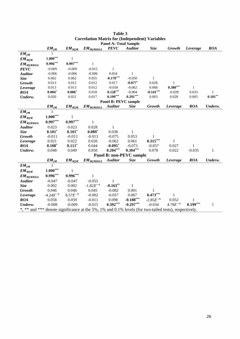
Table 3 reports correlation among the exogenous variables for PEVC and non-PEVC. In
general, correlations are quite low, although some of the correlations are statistically
significant at the 1% level. As expected, PEVC-sponsored IPOs are associated with highly
reputed auditors and underwriters. Moreover, variables Auditor and Underwriter have high
correlation indicating that firms that choses highly reputed auditors also tend to choose highly
reputed underwriters. Large firms tend to hire better underwriter, present higher leverage and
lower ROA. Firms that hire top auditors and underwriters are less indebted.

14
4 METHODOLOGY
4.1 Hypotheses
H1: PEVC-sponsored firms present lower level of earnings management at the time of
the IPO than non- PEVC-sponsored ones.
Teoh et al. (1998b) point that the IPO process gives entrepreneurs both motivation and
opportunities to engage into EM, giving by the fact that there is high information asymmetric
between investors and issuers during the time of the IPO. For instance, Rao (1993) reports the
lack of news media coverage of firms before their IPO. Therefore, prospectus id the main
source of information for IPO. However, prospectuses may contain financial statement for
some few years preceding the IPO. As consequence, investors can hardly rely on historical
data to estimate the extent to which firms engage into EM at the time at the time of the IPO.
For those reasons, managers of issuing firms have both the opportunity and the motivation to
manipulate earnings in order to inflate offering price.
4.2 Regression Model
To test the hypothesis H1, I will use panel regressions where the dependent variable is
the level of EM for firm i at time t, EMi,t (measured by the discretionary current accruals for
firm i at time t). The variable of interest PEVCi, a time unvarying dummy variable assuming
value one when the observation comes from a firm with PECV sponsorship. To confirm H1,
the coefficient of the dummy variable must be negative. The model also includes a number of
control variables that can influence the incentives for earnings manipulation:
𝐸𝑀𝑖, 𝑡 = 𝛽0 + 𝛽1𝑃𝐸𝐶𝑉𝑖 + 𝛽2𝐴𝑢𝑑𝑖𝑡𝑜𝑟 𝑖 + 𝛽4𝑆𝑖𝑧𝑒 𝑖, 𝑡 + 𝛽5𝐺𝑟𝑜𝑤𝑡ℎ 𝑖, 𝑡 + 𝛽6𝐿𝑒𝑣𝑒𝑟𝑎𝑔𝑒 𝑖, 𝑡
+ 𝛽7𝑅𝑂𝐴 + 𝜀 𝑖, 𝑡

15
5 EMPIRICAL RESULTS
In Table 4 the descriptive statistics for the outcome of each of the earnings management
models are reported by the PEVC and non-PEVC categories. In addition, the mean
differences between the two PEVC categories are tested. The 2-tailed t-statistics are given for
each model earnings management proxy, viz. for the Jones (𝑡 = −0.27), Modified Jones (𝑡 =
−0.25), and Modified Jones with ROA (𝑡 = 0.42). However, none of the earnings
management differences are significant at any of the significance levels 1, 5 or 10 per cent. In
the table the number of observations, mean, standard deviation, 25th and 75th percentile
statistics are summarized per model outcome. The total sample consists of 825 firm-quarter
EM observations, the PEVC-sponsored firms sample has 484 observations while the non-
PEVC-sponsored sample has 341 EM observations. The statistics of the Jones and Modified
Jones earnings management are approximately similar. In same way the EMs across all
models do not show very large differences (0.0098 and 0.0097 resp.). The EM variations are
approximately between 36 (0.0098/0.00021) and 47 (0.0097/0.00027) times the mean for the
total sample. The average EM lies below the middle observation for all models (resp. -
0.00021>-0.0009; -0.00027>-0.0010). According to the 25th and 75th percentiles 50 per cent
of the observations lie between the values -0.0040 and 0.0021 with a range of 0.0061 (0.0021
- -0.0040) for the Jones model. The range is resp. 0.0060 and 0.0057 for Modified Jones and
Modified Jones with ROA. The latter model has less value dispersion compared to the other 3
models (0.0057<0.0060<0.0061), with the smallest standard deviation and the largest
absolute mean EM. The mean difference between PEVC and non-PEVC sample for the Jones
(Modified Jones model) is -0.00019 (-0.00018) while this difference is much larger for the
Modified Jones with ROA EM (-0.00029). This larger dissimilarity between the two groups
results in a relatively later t-statistic (0.42) however not sufficiently large significant
16
difference. Figure 1 shows the EM means of the 3 models by sponsor category. Obviously,
the PEVC-sponsored firms have a smaller EM compared to the non-PEVC sample and the
Modified Jones with ROA shows an even smaller EM when sponsored. These findings
suggest that Jones and Modified Jones should not yield different results while the Modified
Jones with ROA is differentiated the most by the dummy variable PEVC.
In Table 5 the results of the OLS regressions for the 3 EM models are reported, for the
pooled and the random effects estimates. The mean difference between the PEVC- and non-
PEVC-sponsored firms EM, namely the beta below each model 1-6 is -0.0002, approximately
similar to the mean EM differences in Table 4 (-0.00019, -0.00018, and -0.00029).
Accordingly, EM is not significantly different between the PEVC and non-PEVC-sponsored
firms, as was revealed in the t-tests above. The firm size in all models is significant with
0.0008 for models 1-4 and 0.0006 for models 5-6. A 1 per cent increase in firm size results in
an increase of 0.0008 (p<5%) and 0.0006 for models 5-6 (p>5%). Thus, models 1-4 provide
the most sensitive EM outcome with respect to the firm size, while models 5-6 react
relatively flatter to size change. The latter two model size betas are insignificant. Dummy
Auditor, firm growth and leverage have no significant impact on the 3 EM proxies (p>5%).
ROA betas are highly significant in model 1-4 with betas 0.0152 and 0.0153 (p<1%). A 1 per
cent in crease of a firm’s scaled net income, increases the EM on average by 0.052 or 0.053.
ROA beta in models 5-6 is insignificant. Except in model 5-6, constants are significant at the
5 per cent level. The constant is the mean EM value for the non-PEVC-sponsored firms,
when controlled for the independent variables in the models. The number of observations for
all estimations is 825, which is the joint number of observations for all model variables.
Model 1-4 (5-6) estimations have an explanatory power – i.e. a 𝑅2 of 1.4 (0.5) per cent. All
models have included quarter dummy variables and the standard errors are clustered by the
firm id, to account for heterogeneous effects between firms. Before performing the random

17
effects estimations, the Hausman test is performed to test for the difference in the betas of the
fixed and random effect panel regressions. The null hypothesis states that both panel
estimates produce same coefficients, which is not rejected as it appears from the p-values
(0.667, 0.671, 0.674). While there are a few independent variables having a significant effect
on the EMs, none of the models are significant. This is shown by the p-value below the F-test
for the pooled OLS and the Wald Chi2 test for the Random effects panel regressions in the
table. All of the p-values are above 5 per cent. While there is sufficient number of
observations and a couple of significant control variables, the model cannot distinguish the
Jones, Modified Jones and Modified Jones with ROA earnings management proxy between
the PEVC and non-PEVC-sponsored firms.

18
6 CONCLUSIONS
Several studies have been concerned with EM at the time of public offerings and the role
of venture capitalists in hampering such practice. Most studies use annual data and, because
of this, do not unveil the dynamics of EM (i.e., the moments at which earnings are inflated
and subsequently deflated). Moreover, the lack such dynamics limits the understanding of the
role played by venture capitalists, i.e., at what moment there is a difference between PEVC
and non-PEVC-sponsored firms and whether such difference is only relative or whether
PEVC-sponsored firms do not manipulate earnings at all. I investigated the behaviour of the
EM in the two main phases: pre-IPO and post-IPO and combined to have an overall of the
EM at the end of those phases. Estimating the EM for each phase, taking four financial
quarters pre-IPO and eight financial quarters post-IPO for each sample (PEVC sponsored and
non-PEVC sponsored firms). As previous explained, in the section “Results”, using the
descriptive statistics, shows that the mean difference between PEVC and non-PEVC sample
for the Jones (Modified Jones model) is -0.00019 (-0.00018) while this difference is much
larger for the Modified Jones with ROA EM (-0.00029). This larger dissimilarity between the
two groups results in a relatively later t-statistic (0.42) however not sufficiently large
significant difference. Figure 1 shows the EM means of the 3 models by sponsor category.
Obviously, the PEVC-sponsored firms have a smaller EM compared to the non-PEVC
sample and the Modified Jones with ROA shows an even smaller EM when sponsored. These
findings suggest that Jones and Modified Jones should not yield different results while the
Modified Jones with ROA is differentiated the most by the dummy variable PEVC.
Moreover, the results from the OLS regressions indicates that the null hypothesis states that
both panel estimates produce same coefficients, which is not rejected as it appears from the p-
values (0.667, 0.671, 0.674). While there are a few independent variables having a significant

19
effect on the EMs, none of the models are significant. This is shown by the p-value below the
F-test for the pooled OLS and the Wald Chi2 test for the Random effects panel regressions in
the table. All of the p-values are above 5 per cent. Comparing to the paper mentioned in the
introduction, is possible to see that there are significant differences regarding the hypothesis
H1, between the two researches. Having a longer sample, in terms of period and financial
quarters and the combination of the results above, brings me to a conclusion that, EM is
shown in non-PEVC sponsored firms, confirming my hypothesis H1 giving by the facts that:
historically ups and downs in term of economy (2000-2015) and strongly relation with
scandals (Corruption-ex. Lula Government or Operation Car Wash) impacted more to
companies related to the public sector and backed as IPO from non-PEVC firms than PEVC.
In a future research, this model could be used with different proxies for the total current
accruals, in combination with different EM models.

20
7 REFERENCES
Angelo, L. E. Accounting numbers as market valuation substitute: a study of management
buyouts of public stockholders. Accounting Review, Jul.1986
Bartov, E.; Gul, F.; Tsui, J. S. L. Discretionary accruals models and audit qualifications.
Journal of Accounting and Economics. Dic.2000
Bloomberg Terminal: IPO data
Dechow, P. M.; Sloan, R.G.; Sweeney, A.P. Detecting earnings management. Accounting
Review. Apr.1995
Economatica: Quarterly financial statements for the IPOs
Healy, P. M., 1985. The effect of bonus schemes on accounting decisions. Journal of
Accounting
and Economics 7, 85-107.
Hochberg, Y. V., 2012. Venture Capital and Corporate Governance in the Newly Public
Firm.
Review of Finance, 16 (2), 429-480.
Jones, J. J., 1991. Earnings management during import relief investigations. Journal of
Accounting Research 29 (2), 193-228.
Kang, S., Sivaramakrishanan, K., 1995. Issues in testing earnings management: an
instrumental
variable approach. Journal of Accounting Research 33 (2), 353-367.
Kothari, S. P., Leone, A. J., Wasley, C. E., 2005. Performance matched discretionary accrual
measures. Journal of Accounting and Economics 39 (1), 163-197.
Leeds, R. (2016). Private equity investing in emerging markets: Opportunities for value
creation. Place of publication not identified: Palgrave Macmillan.
Rangan, S., 1998. Earnings management and the performance of seasoned equity offerings.
Journal of Financial Economics 50 (1), 101-122.
Rao, G. R., 1993. The relation between stock returns and earnings: a study of newly-public
firms.
Working paper, Kidder Peabody and Co., New York.

21
Teoh, S. H., Welch, I., Wong, T. J., 1998. Earnings management and the underperformance
of
seasoned equity offerings. Journal of Financial Economics 50 (1), 101-122.
Teoh, S. H., Welch, I., Wong, T. J., 1998. Earnings management and the long-run market
performance of initial public offerings. Journal of Finance 53 (6), 1935–1974.
Sampaio, J. O.; de Carvalho, A. G.; Gioielli, S. P. O. Venture Capital and earnings
management in IPOs. Brazilian Business Review. Dec.2013
Subramanyan, K. R., 1996. The pricing of discretionary accruals. Journal of Accounting and
Economics 22, 249-281.
22
8 APPENDIX
8.1 Methodology to for Estimating Earning Management
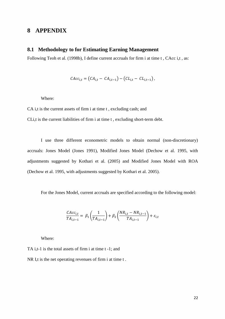
Following Teoh et al. (1998b), I define current accruals for firm i at time t , CAcc i,t , as:
𝐶𝐴𝑐𝑐𝑖,𝑡 = (𝐶𝐴𝑖,𝑡 − 𝐶𝐴𝑖,𝑡−1) − (𝐶𝐿𝑖,𝑡 − 𝐶𝐿𝑖,𝑡−1) ,
Where:
CA i,t is the current assets of firm i at time t , excluding cash; and
CLi,t is the current liabilities of firm i at time t , excluding short-term debt.
I use three different econometric models to obtain normal (non-discretionary)
accruals: Jones Model (Jones 1991), Modified Jones Model (Dechow et al. 1995, with
adjustments suggested by Kothari et al. (2005) and Modified Jones Model with ROA
(Dechow et al. 1995, with adjustments suggested by Kothari et al. 2005).
For the Jones Model, current accruals are specified according to the following model:
𝐶𝐴𝑐𝑐𝑖,𝑡
𝑇𝐴𝑖,𝑡−1= 𝛽1 (
1
𝑇𝐴𝑖,𝑡−1) + 𝛽2 (
𝑁𝑅𝑖,𝑡 − 𝑁𝑅𝑖,𝑡−1
𝑇𝐴𝑖,𝑡−1) + 𝜀𝑖,𝑡
Where:
TA i,t-1 is the total assets of firm i at time t -1; and
NR I,t is the net operating revenues of firm i at time t .

23
For the Modified Jones Model, current accruals are specified according to the
following model:
𝐶𝐴𝑐𝑐𝑖,𝑡
𝑇𝐴𝑖,𝑡−1= 𝛽1 (
1
𝑇𝐴𝑖,𝑡−1) + 𝛽2 (
(𝑁𝑅𝑖,𝑡 − 𝑁𝑅𝑖,𝑡−1) − (𝑇𝑅𝑖,𝑡 − 𝑇𝑅𝑖,𝑡−1)
𝑇𝐴𝑖,𝑡−1) + 𝜀𝑖,𝑡
Where
TR i,t is the trade accounting receivables of firm i at time t .
Finally, for the Modified Jones Model with ROA, current accruals are specified
according to the following model:
𝐶𝐴𝑐𝑐𝑖,𝑡
𝑇𝐴𝑖,𝑡−1= 𝛽1 (
1
𝑇𝐴𝑖,𝑡−1) + 𝛽2 (
(𝑁𝑅𝑖,𝑡 − 𝑁𝑅𝑖,𝑡−1) − (𝑇𝑅𝑖,𝑡 − 𝑇𝑅𝑖,𝑡−1)
𝑇𝐴𝑖,𝑡−1) + 𝛽3(𝑅𝑂𝐴𝑖,𝑡) + 𝜀𝑖,𝑡
Where
ROA i,t, is the return on assets of firm i at time t .
To compute non-discretionary current accruals for IPO firm i at time t, NDCA i,t , we
estimate the regressions above cross-sectionally for a sample (control group) of firms at
quarter t . The control group for each quarter is formed of all firms listed on BM&FBovespa
excluding: 1) financial firms and real-estate investment trusts; 2) firms that trade OTC; 3)
firms that had conducted either an IPO or SEO and were in the IPO or lock-up periods; 4)
firms for which balance sheets were not available in the specific quarter; and 5) firms for
which the accruals were in the 1st and 99th percentiles in the specific quarter (in order to

24
minimize the influence of outliers). For instance, using the Jones Model, non-discretionary
current accruals (NDCA i,t ) are calculated as:
𝑁𝐷𝐶𝐴𝑖,𝑡 = �̂�1 (1
𝑇𝐴𝑖,𝑡−1) + �̂�2 (
𝑁𝑅𝑖,𝑡 − 𝑁𝑅𝑖,𝑡−1
𝑇𝐴𝑖,𝑡−1) + 𝜀𝑖,𝑡
Where:
�̂�1 and �̂�2 are the estimates from the Regression from the Jones Model.
Finally, earnings management for IPO firm i at time t (EM i,t , ) are calculated as the
difference between CAcc i,t , (scaled by lagged total assets) and NDCA i,t :
𝐸𝑀𝑖,𝑡 = 𝐶𝐴𝑐𝑐𝑖,𝑡
𝑇𝐴𝑖,𝑡−1− 𝑁𝐷𝐶𝐴𝑖,𝑡

25
8.2 Tables and Exhibits
Table 2
Descriptive Statistics of Financial Characteristics
The variables: Auditor is a dummy with 1 (0) for big four (non-big four) for each auditing firm 𝑖; Size is
firm 𝑖’s natural logarithm of book value of assets at quarter 𝑡; Growth is firm 𝑖’s % change in net operating
revenues at quarter 𝑡; Leverage is firm 𝑖’s % change in EBIT divided by % change in revenue at quarter 𝑡;
ROA is firm 𝑖’s return on assets calculated by net income divided by the book value of total assets at
quarter 𝑡; Underwr. is underwriter and is firm 𝑖’s Cater-Manaster index of the member of the underwriting
syndicate with the highest score. T-statistics tests the difference in means between PEVC and non-PEVC-
sponsored firms. Bold-faced t-statistics indicates statistically significance at the 1% level. All Firms PEVC-Sponsored Firms Non-PEVC-Sponsored Firms
N=825 N=484 N=341
74 IPOs 44 IPOs 30 IPOs
Mean Median Std. Dev. Mean Median Std. Dev. Mean Median Std. Dev. t-Stat
Auditor 0.70 1.00 0.53 0.73 1.00 0.54 0.67 1.00 0.52 -1.56
Size 14.52 14.49 0.97 14.38 14.38 0.98 14.72 14.67 0.93 4.95
Growth -0.90 -0.71 1.86 -0.87 -0.72 1.80 -0.94 -0.69 1.94 -0.48
Leverage -0.26 -0.10 3.76 -0.36 -0.11 3.84 -0.10 -0.07 3.63 0.98
ROA 0.03 0.03 0.07 0.04 0.03 0.06 0.02 0.02 0.07 -3.71
Underwr. 0.69 1.00 0.52 0.77 1.00 0.47 0.56 1.00 0.56 5.83
26
Table 3
Correlation Matrix for (Independent) Variables
Panel A: Total Sample
𝑬𝑴𝑱𝑴 𝑬𝑴𝑴𝑱𝑴 𝑬𝑴𝑴𝑱𝑴𝑹𝑶𝑨 PEVC Auditor Size Growth Leverage ROA
𝑬𝑴𝑱𝑴 1
𝑬𝑴𝑴𝑱𝑴 1.000*** 1
𝑬𝑴𝑴𝑱𝑴𝑹𝑶𝑨 0.996*** 0.997*** 1
PEVC -0.009 -0.009 -0.015 1
Auditor -0.006 -0.006 -0.006 0.054 1
Size 0.062 0.062 0.055 -0.170*** -0.050 1
Growth 0.013 0.012 0.012 0.017 -0.077* 0.028 1
Leverage 0.013 0.013 0.012 -0.034 -0.062 0.068 0.380*** 1
ROA 0.084* 0.086* 0.018 0.128*** -0.004 -0.141*** -0.028 0.033 1
Underw. 0.020 0.021 0.017 0.199*** 0.291*** 0.003 0.028 0.005 0.101**
Panel B: PEVC sample
𝑬𝑴𝑱𝑴 𝑬𝑴𝑴𝑱𝑴 𝑬𝑴𝑴𝑱𝑴𝑹𝑶𝑨 Auditor Size Growth Leverage ROA Underw.
𝑬𝑴𝑱𝑴 1
𝑬𝑴𝑴𝑱𝑴 1.000*** 1
𝑬𝑴𝑴𝑱𝑴𝑹𝑶𝑨 0.997*** 0.997*** 1
Auditor 0.023 0.023 0.028 1
Size 0.101* 0.101* 0.089* 0.038 1
Growth -0.011 -0.013 -0.013 -0.075 0.053 1
Leverage 0.021 0.022 0.020 -0.062 0.061 0.315*** 1
ROA 0.108* 0.111* 0.044 -0.095* -0.073 -0.057 0.027 1
Underw. 0.048 0.049 0.050 0.204*** 0.304*** 0.078 0.022 -0.035 1
Panel B: non-PEVC sample
𝑬𝑴𝑱𝑴 𝑬𝑴𝑴𝑱𝑴 𝑬𝑴𝑴𝑱𝑴𝑹𝑶𝑨 Auditor Size Growth Leverage ROA Underw.
𝑬𝑴𝑱𝑴 1
𝑬𝑴𝑴𝑱𝑴 1.000*** 1
𝑬𝑴𝑴𝑱𝑴𝑹𝑶𝑨 0.996*** 0.996*** 1
Auditor -0.047 -0.047 -0.055 1
Size 0.002 0.002 -1.82𝐸−4 -0.163** 1
Growth 0.046 0.046 0.045 -0.082 0.001 1
Leverage -4.24𝐸−5 8.57𝐸−5 -0.002 -0.057 0.067 0.473*** 1
ROA 0.058 0.059 -0.011 0.098 -0.188*** -2.85𝐸−6 0.052 1
Underw. -0.008 -0.009 -0.015 0.392*** -0.297*** -0.034 4.78𝐸−4 0.199*** 1
*, ** and *** denote significance at the 5%, 1% and 0.1% levels (for two-tailed tests), respectively.

27
Figure 1
Table 4
Earnings management in PEVC and Non-PEVC
Descriptive statistics for the level of earnings management (EM). The sample consists of 825 firm-
quarter observations from 74 IPOs at BM & FBovespa from 30 September 2004 to 30 September 2017.
The three measurements of EM are based on Jones, Modified Jones and Modified Jones with ROA
models. EM is in percentage of total assets. None of the differences are significant.
Model Sample N Mean Standard
Deviation
25th
percentile Median
75th
percen
tile
Jones
All observations 825 -0.00021 0.0098 -0.0040 -0.0009 0.0021
PEVC-Sponsored 484 -0.00029 0.0098 -0.0040 -0.0008 0.0021
Non-PEVC-Sponsored 341 -0.00010 0.0098 -0.0037 -0.0010 0.0021
Difference -0.00019 𝑡 −Statistic = -0.27
Modifie
d Jones
All observations 825 -0.00021 0.0098 -0.0040 -0.0009 0.0020
PEVC-Sponsored 484 -0.00029 0.0098 -0.0041 -0.0008 0.0020
Non-PEVC-Sponsored 341 -0.00011 0.0098 -0.0037 -0.0011 0.0021
Difference -0.00018 𝑡 −Statistic = -0.25
Modifie
d Jones
with
ROA
All observations 825 -0.00027 0.0097 -0.0039 -0.0010 0.0018
PEVC-Sponsored 484 -0.00039 0.0097 -0.0042 -0.0009 0.0018
Non-PEVC-Sponsored 341 -0.00010 0.0098 -0.0036 -0.0011 0.0020
Difference -0.00029 𝑡 −Statistic = 0.42

28
Table 5
PEVC-Sponsorship and Earnings Management
Panel regressions analysis. The dependent variable is earnings management for firm 𝑖 in the quarter 𝑡 as
percentage of the total assets. It was calculated using three different models (Jones, Modified Jones and
Modified Jones with ROA). The sample consists of 825 firm-quarter observations from 74 IPOs at
BM&FBovespa from 30 September 2004 to 30 September 2017. Robust heteroskedastic-consistent
standard errors are between parentheses.
Jones Modified Jones Modified Jones with ROA
Variable Pooled
OLS
Random
Effects
Pooled
OLS
Random
Effects
Pooled
OLS
Random
Effects
Model: (1) (2) (3) (4) (5) (6)
PEVC -0.0002 -0.0002 -0.0002 -0.0002 -0.0002 -0.0002
(0.0007) (0.0007) (0.0007) (0.0007) (0.0007) (0.0007)
Auditor -0.0000 -0.0000 -0.0000 -0.0000 -0.0000 -0.0000
(0.0005) (0.0005) (0.0005) (0.0005) (0.0005) (0.0005)
Size 0.0008** 0.0008** 0.0008** 0.0008** 0.0006* 0.0006*
(0.0003) (0.0003) (0.0003) (0.0003) (0.0003) (0.0003)
Growth -0.0000 -0.0000 0.0000 0.0000 0.0000 0.0000
(0.0002) (0.0002) (0.0002) (0.0002) (0.0002) (0.0002)
Leverage 0.0000 0.0000 0.0000 0.0000 0.0000 0.0000
(0.0001) (0.0001) (0.0001) (0.0001) (0.0001) (0.0001)
ROA 0.0152*** 0.0152*** 0.0153*** 0.0153*** 0.0043 0.0043
(0.0055) (0.0055) (0.0055) (0.0055) (0.0053) (0.0053)
Constant -0.0111** -0.0111** -0.0113** -0.0113** -0.0085* -0.0085*
(0.0048) (0.0048) (0.0048) (0.0048) (0.0048) (0.0048)
Quarter Dummies Yes Yes Yes Yes Yes Yes
Firm Clusters Yes Yes Yes Yes Yes Yes
# of Observations 825 825 825 825 825 825
𝑅2 0.014 0.014 0.014 0.014 0.005 0.005
F-Test (Pooled OLS) and Wald Chi2test (Random Effects)
Statistic 1.684 15.155 1.692 15.230 0.547 4.919
p-value 0.108 0.713 0.106 0.708 0.836 0.999
Hausman Test for Random Effects
p-value 0.667 0.671 0.674
*, ** and *** denote significance at the 10%, 5% and 1% levels (for two-tailed tests), respectively.
Hausman test: The null is that the two estimation methods are both OK and that therefore they
should yield coefficients that are "similar". The alternative hypothesis is that the fixed effects
estimation is OK, and the random effects estimation is not; if this is the case, then we would expect to
see differences between the two sets of coefficients.
What this text above is saying is that both fixed and random effects regression are ok.

29
Exhibits 1: Brazil Private Equity Fundraising, 2002-2008 (US$ Billions)

30
Exhibits 2: Latin America Private Equity Fundraising, 2004-2008 (US$ Billions)
Exhibits 3: Private Equity Fundraising and Investment in Brazil, 2009-2013 (US$ Billions)