Priority Queues and Heapsort MANY APPLICATIONS REQUIRE ... · Priority Queues and Heapsort MANY APPLICATIONS REQUIRE that we process records with keys in order, but not necessarily

C H A P T E R N I N E

Priority Queues and Heapsort

M ANY APPLICATIONS REQUIRE that we process records withkeys in order, but not necessarily in full sorted order and not

necessarily all at once. Often, we collect a set of records, then processthe one with the largest key, then perhaps collect more records, thenprocess the one with the current largest key, and so forth. An appropri-ate data structure in such an environment supports the operations ofinserting a new element and deleting the largest element. Such a datastructure is called a priority queue. Using priority queues is similarto using queues (remove the oldest) and stacks (remove the newest),but implementing them efficiently is more challenging. The priorityqueue is the most important example of the generalized queue ADTthat we discussed in Section 4.7. In fact, the priority queue is a propergeneralization of the stack and the queue, because we can implementthese data structures with priority queues, using appropriate priorityassignments (see Exercises 9.3 and 9.4).

Definition 9.1 A priority queue is a data structure of items with keyswhich supports two basic operations: insert a new item, and removethe item with the largest key.

Applications of priority queues include simulation systems, where thekeys might correspond to event times, to be processed in chronologi-cal order; job scheduling in computer systems, where the keys mightcorrespond to priorities indicating which users are to be served first;and numerical computations, where the keys might be computationalerrors, indicating that the largest should be dealt with first.

373

374 C H A P T E R N I N E

We can use any priority queue as the basis for a sorting algorithmby inserting all the records, then successively removing the largest toget the records in reverse order. Later on in this book, we shall seehow to use priority queues as building blocks for more advanced algo-rithms. In Part 5, we shall see how priority queues are an appropriateabstraction for helping us understand the relationships among severalfundamental graph-searching algorithms; and in Part 6, we shall de-velop a file-compression algorithm using routines from this chapter.These are but a few examples of the important role played by thepriority queue as a basic tool in algorithm design.

In practice, priority queues are more complex than the simpledefinition just given, because there are several other operations thatwe may need to perform to maintain them under all the conditionsthat might arise when we are using them. Indeed, one of the mainreasons that many priority-queue implementations are so useful is theirflexibility in allowing client application programs to perform a varietyof different operations on sets of records with keys. We want to buildand maintain a data structure containing records with numerical keys(priorities) that supports some of the following operations:• Construct a priority queue from N given items.• Insert a new item.• Remove the maximum item.• Change the priority of an arbitrary specified item.• Remove an arbitrary specified item.• Join two priority queues into one large one.

If records can have duplicate keys, we take “maximum” to mean “anyrecord with the largest key value.” As with many data structures, wealso need to add a standard test if empty operation and perhaps a copy(clone) operation to this set.

There is overlap among these operations, and it is sometimes con-venient to define other, similar operations. For example, certain clientsmay need frequently to find the maximum item in the priority queue,without necessarily removing it. Or, we might have an operation toreplace the maximum item with a new item. We could implementoperations such as these using our two basic operations as buildingblocks: Find the maximum could be remove the maximum followedby insert, and replace the maximum could be either insert followed byremove the maximum or remove the maximum followed by insert. We

P R I O R I T Y Q U E U E S A N D H E A P S O R T 375

Program 9.1 Basic priority-queue ADT

This interface defines operations for the simplest type of priority queue:initialize, test if empty, add a new item, remove the largest item. Elemen-tary implementations of these methods using arrays and linked lists canrequire linear time in the worst case, but we shall see implementationsin this chapter where all operations are guaranteed to run in time atmost proportional to the logarithm of the number of items in the queue.The constructor’s parameter specifies the maximum number of itemsexpected in the queue and may be ignored by some implementations.

class PQ // ADT interface

{ // implementations and private members hidden

PQ(int)

boolean empty()

void insert(ITEM)

ITEM getmax()

};

normally get more efficient code, however, by implementing such op-erations directly, provided that they are needed and precisely specified.Precise specification is not always as straightforward as it might seem.For example, the two options just given for replace the maximum arequite different: the former always makes the priority queue grow tem-porarily by one item, and the latter always puts the new item on thequeue. Similarly, the change priority operation could be implementedas a remove followed by an insert, and construct could be implementedwith repeated uses of insert.

For some applications, it might be slightly more convenient toswitch around to work with the minimum, rather than with the maxi-mum. We stick primarily with priority queues that are oriented towardaccessing the maximum key. When we do need the other kind, we shallrefer to it (a priority queue that allows us to remove the minimum item)as a minimum-oriented priority queue.

The priority queue is a prototypical abstract data type (ADT) (seeChapter 4): It represents a well-defined set of operations on data, andit provides a convenient abstraction that allows us to separate appli-cations programs (clients) from various implementations that we willconsider in this chapter. The interface given in Program 9.1 defines themost basic priority-queue operations; we shall consider a more com-

376 C H A P T E R N I N E

plete interface in Section 9.5. Strictly speaking, different subsets ofthe various operations that we might want to include lead to differentabstract data structures, but the priority queue is essentially character-ized by the remove-the-maximum and insert operations, so we shallfocus on them.

Different implementations of priority queues afford different per-formance characteristics for the various operations to be performed,and different applications need efficient performance for different setsof operations. Indeed, performance differences are, in principle, theonly differences that can arise in the abstract-data-type concept. Thissituation leads to cost tradeoffs. In this chapter, we consider a vari-ety of ways of approaching these cost tradeoffs, nearly reaching theideal of being able to perform the remove the maximum operation inlogarithmic time and all the other operations in constant time.

First, in Section 9.1, we illustrate this point by discussing a fewelementary data structures for implementing priority queues. Next,in Sections 9.2 through 9.4, we concentrate on a classical data struc-ture called the heap, which allows efficient implementations of all theoperations but join. In Section 9.4, we also look at an importantsorting algorithm that follows naturally from these implementations.In Sections 9.5 and 9.6, we look in more detail at some of the prob-lems involved in developing complete priority-queue ADTs. Finally,in Section 9.7, we examine a more advanced data structure, called thebinomial queue, that we use to implement all the operations (includingjoin) in worst-case logarithmic time.

During our study of all these various data structures, we shallbear in mind both the basic tradeoffs dictated by linked versus sequen-tial memory allocation (as introduced in Chapter 3) and the problemsinvolved with making packages usable by applications programs. Inparticular, some of the advanced algorithms that appear later in thisbook are client programs that make use of priority queues.

Exercises

.9.1 A letter means insert and an asterisk means remove the maximum inthe sequence

P R I O * R * * I * T * Y * * * Q U E * * * U * E.

Give the sequence of values returned by the remove the maximum operations.

.9.2 Add to the conventions of Exercise 9.1 a plus sign to mean join andparentheses to delimit the priority queue created by the operations within

P R I O R I T Y Q U E U E S A N D H E A P S O R T §9.1 377

them. Give the contents of the priority queue after the sequence

( ( ( P R I O *) + ( R * I T * Y * ) ) * * * ) + ( Q U E * * * U * E ).

◦9.3 Explain how to use a priority queue ADT to implement a stack ADT.

◦9.4 Explain how to use a priority queue ADT to implement a queue ADT.

9.1 Elementary Implementations

The basic data structures that we discussed in Chapter 3 provide uswith numerous options for implementing priority queues. Program 9.2is an implementation that uses an unordered array as the underlyingdata structure. The find the maximum operation is implemented byscanning the array to find the maximum, then exchanging the maxi-mum item with the last item and decrementing the queue size. Fig-ure 9.1 shows the contents of the array for a sample sequence ofoperations. This basic implementation corresponds to similar im-plementations that we saw in Chapter 4 for stacks and queues (seePrograms 4.7 and 4.17) and is useful for small queues. The significantdifference has to do with performance. For stacks and queues, wewere able to develop implementations of all the operations that takeconstant time; for priority queues, it is easy to find implementationswhere either the insert or the remove the maximum operations takesconstant time, but finding an implementation where both operationswill be fast is a more difficult task, and it is the subject of this chapter.

We can use unordered or ordered sequences, implemented aslinked lists or as arrays. The basic tradeoff between leaving the itemsunordered and keeping them in order is that maintaining an orderedsequence allows for constant-time remove the maximum and find themaximum but might mean going through the whole list for insert,whereas an unordered sequence allows a constant-time insert but mightmean going through the whole sequence for remove the maximum andfind the maximum. The unordered sequence is the prototypical lazyapproach to this problem, where we defer doing work until necessary(to find the maximum); the ordered sequence is the prototypical eagerapproach to the problem, where we do as much work as we canup front (keep the list sorted on insertion) to make later operationsefficient. We can use an array or linked-list representation in eithercase, with the basic tradeoff that the (doubly) linked list allows a

378 §9.1 C H A P T E R N I N E

B BE B E* E BS B ST B S TI B S T I* T B S IN L S I N* S B N IF B N I FI B N I F IR B N I F I R* R B N I F IS B N I F I ST B N I F I S T* T B N I F I S* S B N I F IO B N I F I OU B N I F I O U* U B N I F I OT B N I F I O T* T B N I F I O* O B N I F I* N B I I F* I B F I* I B F* F B* B

Figure 9.1Priority-queue example (un-

ordered array representa-tion)

This sequence shows the result ofthe sequence of operations in theleft column (top to bottom), wherea letter denotes insert and an aster-isk denotes remove the maximum.Each line displays the operation,the letter removed for the remove-the-maximum operations, and thecontents of the array after the oper-ation.

Program 9.2 Array implementation of a priority queue

This implementation, which may be compared with the array imple-mentations for stacks and queues that we considered in Chapter 4 (seePrograms 4.7 and 4.17), keeps the items in an unordered array. Itemsare added to and removed from the end of the array, as in a stack.

class PQ{

static boolean less(ITEM v, ITEM w)

{ return v.less(w); }

static void exch(ITEM[] a, int i, int j)

{ ITEM t = a[i]; a[i] = a[j]; a[j] = t; }

private ITEM[] pq;

private int N;

PQ(int maxN)

{ pq = new ITEM[maxN]; N = 0; }

boolean empty()

{ return N == 0; }

void insert(ITEM item)

{ pq[N++] = item; }

ITEM getmax(){ int max = 0;

for (int j = 1; j < N; j++)

if (less(pq[max], pq[j])) max = j;

exch(pq, max, N-1);

return pq[--N];

}

};

constant-time remove (and, in the unordered case, join), but requiresmore space for the links.

The worst-case costs of the various operations (within a constantfactor) on a priority queue of size N for various implementations aresummarized in Table 9.1.

Developing a full implementation requires paying careful atten-tion to the interface—particularly to how client programs access nodesfor the remove and change priority operations, and how they accesspriority queues themselves as data types for the join operation. These


Table 9.1 Worst-case costs of priority-queue operations

Implementations of the priority queue ADT have widely varying perfor-mance characteristics, as indicated in this table of the worst-case time(within a constant factor for large N) for various methods. Elementarymethods (first four lines) require constant time for some operations andlinear time for others; more advanced methods guarantee logarithmic-or constant-time performance for most or all operations.

remove find changeinsert maximum remove maximum priority join

ordered array N 1 N 1 N N

ordered list N 1 1 1 N N

unordered array 1 N 1 N 1 N

unordered list 1 N 1 N 1 1

heap lgN lgN lgN 1 lgN N

binomial queue lgN lgN lgN lgN lgN lgN

best in theory 1 lgN lgN 1 1 1

issues are discussed in Sections 9.4 and 9.7, where two full implemen-tations are given: one using doubly linked unordered lists, and anotherusing binomial queues.

The running time of a client program using priority queues de-pends not just on the keys but also on the mix of the various operations.It is wise to keep in mind the simple implementations because theyoften can outperform more complicated methods in many practicalsituations. For example, the unordered-list implementation might beappropriate in an application where only a few remove the maximumoperations are performed, as opposed to a huge number of insertions,whereas an ordered list would be appropriate if a huge number of findthe maximum operations are involved, or if the items inserted tend tobe larger than those already in the priority queue.

Exercises

.9.5 Criticize the following idea: To implement find the maximum in con-stant time, why not keep track of the maximum value inserted so far, thenreturn that value for find the maximum?

380 §9.1 C H A P T E R N I N E

.9.6 Give the contents of the array after the execution of the sequence ofoperations depicted in Figure 9.1.

9.7 Provide an implementation for the basic priority-queue interface thatuses an ordered array for the underlying data structure.

9.8 Provide an implementation for the basic priority-queue interface thatuses an unordered linked list for the underlying data structure. Hint: SeePrograms 4.8 and 4.16.

9.9 Provide an implementation for the basic priority-queue interface thatuses an ordered linked list for the underlying data structure. Hint: See Pro-gram 3.11.

◦9.10 Consider a lazy implementation where the list is ordered only when aremove the maximum or a find the maximum operation is performed. Inser-tions since the previous sort are kept on a separate list, then are sorted andmerged in when necessary. Discuss advantages of such an implementationover the elementary implementations based on unordered and ordered lists.

• 9.11 Write a performance driver client program that uses insert to fill apriority queue, then uses getmax to remove half the keys, then uses insertto fill it up again, then uses getmax to remove all the keys, doing so multipletimes on random sequences of keys of various lengths ranging from small tolarge; measures the time taken for each run; and prints out or plots the averagerunning times.

• 9.12 Write a performance driver client program that uses insert to fill apriority queue, then does as many getmax and insert operations as it can doin 1 second, doing so multiple times on random sequences of keys of variouslengths ranging from small to large; and prints out or plots the average numberof getmax operations it was able to do.

9.13 Use your client program from Exercise 9.12 to compare the unordered-array implementation in Program 9.2 with your unordered-list implementa-tion from Exercise 9.8.

9.14 Use your client program from Exercise 9.12 to compare your ordered-array and ordered-list implementations from Exercises 9.7 and 9.9.

• 9.15 Write an exercise driver client program that uses the methods in ourpriority-queue interface Program 9.1 on difficult or pathological cases thatmight turn up in practical applications. Simple examples include keys that arealready in order, keys in reverse order, all keys the same, and sequences of keyshaving only two distinct values.

9.16 (This exercise is 24 exercises in disguise.) Justify the worst-case boundsfor the four elementary implementations that are given in Table 9.1, by ref-erence to the implementation in Program 9.2 and your implementations fromExercises 9.7 through 9.9 for insert and remove the maximum; and by infor-mally describing the methods for the other operations. For remove, changepriority, and join, assume that you have a handle that gives you direct accessto the referent.


X

T O

G S M N

A E R A I

1 1

2 2 3 3

4 4 5 5 6 6 7 7

8 8 9 9 1010 1111 1212

Figure 9.2Array representation of a

heap-ordered completebinary tree

1 2 3 4 5 6 7 8 9 10 11 12X T O G S M N A E R A I

Considering the element in posi-tion bi/2c in an array to be theparent of the element in positioni, for 2 ≤ i ≤ N (or, equiva-lently, considering the ith elementto be the parent of the 2ith ele-ment and the (2i + 1)st element),corresponds to a convenient rep-resentation of the elements as atree. This correspondence is equiv-alent to numbering the nodes in acomplete binary tree (with nodeson the bottom as far left as possi-ble) in level order. A tree is heap-ordered if the key in any givennode is greater than or equal tothe keys of that node’s children. Aheap is an array representation of acomplete heap-ordered binary tree.The ith element in a heap is largerthan or equal to both the 2ith andthe (2i+ 1)st elements.

9.2 Heap Data Structure

The main topic of this chapter is a simple data structure called theheap that can efficiently support the basic priority-queue operations.In a heap, the records are stored in an array such that each key isguaranteed to be larger than the keys at two other specific positions.In turn, each of those keys must be larger than two more keys, and soforth. This ordering is easy to see if we view the keys as being in abinary tree structure with edges from each key to the two keys knownto be smaller.

Definition 9.2 A tree is heap-ordered if the key in each node islarger than or equal to the keys in all of that node’s children (if any).Equivalently, the key in each node of a heap-ordered tree is smallerthan or equal to the key in that node’s parent (if any).

Property 9.1 No node in a heap-ordered tree has a key larger thanthe key at the root.

We could impose the heap-ordering restriction on any tree. It is partic-ularly convenient, however, to use a complete binary tree. Recall fromChapter 3 that we can draw such a structure by placing the root nodeand then proceeding down the page and from left to right, connect-ing two nodes beneath each node on the previous level until N nodeshave been placed. We can represent complete binary trees sequentiallywithin an array by simply putting the root at position 1, its children atpositions 2 and 3, the nodes at the next level in positions 4, 5, 6 and7, and so on, as illustrated in Figure 9.2.

Definition 9.3 A heap is a set of nodes with keys arranged in acomplete heap-ordered binary tree, represented as an array.

We could use a linked representation for heap-ordered trees, but com-plete trees provide us with the opportunity to use a compact arrayrepresentation where we can easily get from a node to its parent andchildren without needing to maintain explicit links. The parent ofthe node in position i is in position bi/2c, and, conversely, the twochildren of the node in position i are in positions 2i and 2i+ 1. Thisarrangement makes traversal of such a tree even easier than if the treewere implemented with a linked representation, because, in a linkedrepresentation, we would need to have three links associated with eachkey to allow travel up and down the tree (each element would have

382 §9.2 C H A P T E R N I N E

one pointer to its parent and one to each child). Complete binary treesrepresented as arrays are rigid structures, but they have just enoughflexibility to allow us to implement efficient priority-queue algorithms.

We shall see in Section 9.3 that we can use heaps to implementall the priority-queue operations (except join) such that they requirelogarithmic time in the worst case. The implementations all operatealong some path inside the heap (moving from parent to child towardthe bottom or from child to parent toward the top, but not switchingdirections). As we discussed in Chapter 3, all paths in a complete treeofN nodes have about lgN nodes on them: there are aboutN/2 nodeson the bottom, N/4 nodes with children on the bottom, N/8 nodeswith grandchildren on the bottom, and so forth. Each generation hasabout one-half as many nodes as the next, and there are at most lgNgenerations.

We can also use explicit linked representations of tree structuresto develop efficient implementations of the priority-queue operations.Examples include triply linked heap-ordered complete trees (see Sec-tion 9.5), tournaments (see Program 5.19), and binomial queues (seeSection 9.7). As with simple stacks and queues, one important reasonto consider linked representations is that they free us from having toknow the maximum queue size ahead of time, as is required with anarray representation. In certain situations, we also can make use ofthe flexibility provided by linked structures to develop efficient algo-rithms. Readers who are inexperienced with using explicit tree struc-tures are encouraged to read Chapter 12 to learn basic methods for theeven more important symbol-table ADT implementation before tack-ling the linked tree representations discussed in the exercises in thischapter and in Section 9.7. However, careful consideration of linkedstructures can be reserved for a second reading, because our primarytopic in this chapter is the heap (linkless array representation of theheap-ordered complete tree).

Exercises.9.17 Is an array that is sorted in descending order a heap?

◦9.18 The largest element in a heap must appear in position 1, and the secondlargest element must be in position 2 or position 3. Give the list of positions ina heap of size 15 where the kth largest element (i) can appear, and (ii) cannotappear, for k = 2, 3, 4 (assuming the values to be distinct).

• 9.19 Answer Exercise 9.18 for general k, as a function of N , the heap size.


• 9.20 Answer Exercises 9.18 and 9.19 for the kth smallest element.

9.3 Algorithms on Heaps

The priority-queue algorithms on heaps all work by first making asimple modification that could violate the heap condition, then trav-eling through the heap, modifying the heap as required to ensure thatthe heap condition is satisfied everywhere. This process is sometimescalled heapifying, or just fixing the heap. There are two cases. Whenthe priority of some node is increased (or a new node is added at thebottom of a heap), we have to travel up the heap to restore the heapcondition. When the priority of some node is decreased (for example,if we replace the node at the root with a new node), we have to traveldown the heap to restore the heap condition. First, we consider howto implement these two basic methods; then, we see how to use themto implement the various priority-queue operations.

If the heap property is violated because a node’s key becomeslarger than that node’s parent’s key, then we can make progress towardfixing the violation by exchanging the node with its parent. After theexchange, the node is larger than both its children (one is the oldparent, and the other is smaller than the old parent because it was achild of that node) but may still be larger than its parent. We can fixthat violation in the same way, and so forth, moving up the heap untilwe reach a node with a larger key, or the root. An example of thisprocess is shown in Figure 9.3. The code is straightforward, basedon the notion that the parent of the node at position k in a heap isat position k/2. Program 9.3 is an implementation of a method thatrestores a possible violation due to increased priority at a given nodein a heap by moving up the heap.

If the heap property is violated because a node’s key becomessmaller than one or both of that node’s childrens’ keys, then we canmake progress toward fixing the violation by exchanging the node withthe larger of its two children. This switch may cause a violation atthe child; we fix that violation in the same way, and so forth, movingdown the heap until we reach a node with both children smaller, orthe bottom. An example of this process is shown in Figure 9.4. Thecode again follows directly from the fact that the children of the nodeat position k in a heap are at positions 2k and 2k+1. Program 9.4 is an

384 §9.3 C H A P T E R N I N E

X

T P

G S O N

A E R A I M

X

S P

G R O N

A E T A I M

Figure 9.3Bottom-up heapify (swim)The tree depicted on the top isheap-ordered except for the nodeT on the bottom level. If we ex-change T with its parent, the treeis heap-ordered, except possiblythat T may be larger than its newparent. Continuing to exchange Twith its parent until we encounterthe root or a node on the pathfrom T to the root that is largerthan T, we can establish the heapcondition for the whole tree. Wecan use this procedure as the basisfor the insert operation on heaps inorder to reestablish the heap con-dition after adding a new elementto a heap (at the rightmost positionon the bottom level, starting a newlevel if necessary).

Program 9.3 Bottom-up heapify

To restore the heap condition when an item’s priority is increased, wemove up the heap, exchanging the item at position k with its parent (atposition k/2) if necessary, continuing as long as the item at position k/2is less than the node at position k or until we reach the top of the heap.The methods less and exch compare and exchange (respectively) theitems at the heap indices specified by their parameters (see Program 9.5for implementations).

private void swim(int k)

{

while (k > 1 && less(k/2, k))

{ exch(k, k/2); k = k/2; }

}

implementation of a method that restores a possible violation due toincreased priority at a given node in a heap by moving down the heap.This method needs to know the size of the heap (N) in order to be ableto test when it has reached the bottom.

These two operations are independent of the way that the treestructure is represented, as long as we can access the parent (for thebottom-up method) and the children (for the top-down method) of anynode. For the bottom-up method, we move up the tree, exchangingthe key in the given node with the key in its parent until we reachthe root or a parent with a larger (or equal) key. For the top-downmethod, we move down the tree, exchanging the key in the givennode with the largest key among that node’s children, moving downto that child, and continuing down the tree until we reach the bottomor a point where no child has a larger key. Generalized in this way,these operations apply not just to complete binary trees but also toany tree structure. Advanced priority-queue algorithms usually usemore general tree structures but rely on these same basic operations tomaintain access to the largest key in the structure, at the top.

If we imagine the heap to represent a corporate hierarchy, witheach of the children of a node representing subordinates (and the par-ent representing the immediate superior), then these operations haveamusing interpretations. The bottom-up method corresponds to apromising new manager arriving on the scene, being promoted up


XT P

G S O N

A E R A I M

OT X

G S P N

A E R A I M

Figure 9.4Top-down heapify (sink)The tree depicted on the top isheap-ordered, except at the root. Ifwe exchange the O with the largerof its two children (X), the tree isheap-ordered, except at the sub-tree rooted at O. Continuing to ex-change O with the larger of its twochildren until we reach the bottomof the heap or a point where O islarger than both its children, wecan establish the heap conditionfor the whole tree. We can use thisprocedure as the basis for the re-move the maximum operation onheaps in order to reestablish theheap condition after replacing thekey at the root with the rightmostkey on the bottom level.

Program 9.4 Top-down heapify

To restore the heap condition when a node’s priority is decreased, wemove down the heap, exchanging the node at position k with the largerof that node’s two children if necessary and stopping when the node atk is not smaller than either child or the bottom is reached. Note that ifN is even and k is N/2, then the node at k has only one child—this casemust be treated properly!

The inner loop in this program has two distinct exits: one for thecase that the bottom of the heap is hit, and another for the case that theheap condition is satisfied somewhere in the interior of the heap. It is aprototypical example of the need for the break construct.

private void sink(int k, int N)

{

while (2*k <= N)

{ int j = 2*k;

if (j < N && less(j, j+1)) j++;

if (!less(k, j)) break;

exch(k, j); k = j;

}

}

the chain of command (by exchanging jobs with any lower-qualifiedboss) until the new person encounters a higher-qualified boss. Mixingmethaphors, we also think about the new arrival having to swim tothe surface. The top-down method is analogous to the situation whenthe president of the company is replaced by someone less qualified.If the president’s most powerful subordinate is stronger than the newperson, they exchange jobs, and we move down the chain of com-mand, demoting the new person and promoting others until the levelof competence of the new person is reached, where there is no higher-qualified subordinate (this idealized scenario is rarely seen in the realworld). Again mixing metaphors, we also think about the new personhaving to sink to the bottom.

These two basic operations allow efficient implementation of thebasic priority-queue ADT, as given in Program 9.5. With the priorityqueue represented as a heap-ordered array, using the insert operationamounts to adding the new element at the end and moving that elementup through the heap to restore the heap condition; the remove the

386 §9.3 C H A P T E R N I N E

SA O

SA

A

TS O

A R I N

TS O

A R I

TS O

A R

S

R O

A

TS O

G R I N

A

Figure 9.5Top-down heap constructionThis sequence depicts the insertionof the keys A S O R T I N G intoan initially empty heap. New itemsare added to the heap at the bot-tom, moving from left to right onthe bottom level. Each insertionaffects only the nodes on the pathbetween the insertion point andthe root, so the cost is proportionalto the logarithm of the size of theheap in the worst case.

Program 9.5 Heap-based priority queue

To implement insert, we increment N, add the new element at the end,then use swim to restore the heap condition. For getmax we take thevalue to be returned from pq[1], then decrement the size of the heap bymoving pq[N] to pq[1] and using sink to restore the heap condition.The first position in the array, pq[0], is not used.

class PQ

{private boolean less(int i, int j)

{ return pq[i].less(pq[j]); }

private void exch(int i, int j)

{ ITEM t = pq[i]; pq[i] = pq[j]; pq[j] = t; }


// Program 9.3


// Program 9.4

private ITEM[] pq;

private int N;

PQ(int maxN)

{ pq = new ITEM[maxN+1]; N = 0; }

boolean empty()

{ return N == 0; }void insert(ITEM v)

{ pq[++N] = v; swim(N); }

ITEM getmax()

{ exch(1, N); sink(1, N-1); return pq[N--]; }

};

maximum operation amounts to taking the largest value off the top,then putting in the item from the end of the heap at the top and movingit down through the array to restore the heap condition.

Property 9.2 The insert and remove the maximum operations forthe priority queue abstract data type can be implemented with heap-ordered trees such that insert requires no more than lgN comparisonsand remove the maximum no more than 2 lgN comparisons, whenperformed on an N -item queue.


XT P

G S O NA E R A I M L E

XT P

G S O NA E R A I M L

XT P

G S O NA E R A I M

XT O

G S M NA E R A I

XT O

G S I NA E R A

XT O

G S I NA E R

TS O

G R I NA E

Figure 9.6Top-down heap construction

(continued)This sequence depicts insertion ofthe keys E X A M P L E into theheap started in Figure 9.5. The to-tal cost of constructing a heap ofsize N is less than

lg 1 + lg 2 + . . .+ lgN,which is less than N lgN .

Both operations involve moving along a path between the root and thebottom of the heap, and no path in a heap of sizeN includes more thanlgN elements (see, for example, Property 5.8 and Exercise 5.77). Theremove the maximum operation requires two comparisons for eachnode: one to find the child with the larger key, the other to decidewhether that child needs to be promoted.

Figures 9.5 and 9.6 show an example in which we construct aheap by inserting items one by one into an initially empty heap. In thearray representation that we have been using for the heap, this processcorresponds to heap ordering the array by moving sequentially throughthe array, considering the size of the heap to grow by 1 each time thatwe move to a new item, and using swim to restore the heap order. Theprocess takes time proportional to N logN in the worst case (if eachnew item is the largest seen so far, it travels all the way up the heap),but it turns out to take only linear time on the average (a random newitem tends to travel up only a few levels). In Section 9.4 we shall see away to construct a heap (to heap order an array) in linear worst-casetime.

The basic swim and sink operations in Programs 9.3 and 9.4also allow direct implementation for the change priority and removeoperations. To change the priority of an item somewhere in the mid-dle of the heap, we use swim to move up the heap if the priority isincreased, and sink to go down the heap if the priority is decreased.Full implementations of such operations, which refer to specific dataitems, make sense only if a handle is maintained for each item to thatitem’s place in the data structure. In order to do so, we need to de-fine an ADT for that purpose. We shall consider such an ADT andcorresponding implementations in detail in Sections 9.5 through 9.7.

Property 9.3 The change priority, remove, and replace the max-imum operations for the priority queue abstract data type can beimplemented with heap-ordered trees such that no more than 2 lgNcomparisons are required for any operation on an N -item queue.

Since they require handles to items, we defer considering implementa-tions that support these operations to Section 9.6 (see Program 9.12and Figure 9.14). They all involve moving along one path in the heap,perhaps all the way from top to bottom or from bottom to top in theworst case.

388 §9.3 C H A P T E R N I N E

NM I

G L E AA E

OM N

G L I AA E E

PM O

G L I NA E E A

RM P

G L O NA E E A I

SR P

G L O NA E E A I M

TS P

G R O NA E E A I M L

XT P

G S O NA E R A I M L E

Figure 9.7Sorting from a heapAfter replacing the largest elementin the heap by the rightmost ele-ment on the bottom level, we canrestore the heap order by siftingdown along a path from the root tothe bottom.

Program 9.6 Sorting with a priority queue

This class uses our priority-queue ADT to implement the standard Sortclass that was introduced in Program 6.3.

To sort a subarray a[l], . . . , a[r], we construct a priority queuewith enough capacity to hold all of its items, use insert to put all theitems on the priority queue, and then use getmax to remove them, indecreasing order. This sorting algorithm runs in time proportional toN lgN but uses extra space proportional to the number of items to besorted (for the priority queue).

class Sort

{

static void sort(ITEM[] a, int l, int r)

{ PQsort(a, l, r); }

static void PQsort(ITEM[] a, int l, int r)

{ int k;

PQ pq = new PQ(r-l+1);

for (k = l; k <= r; k++)

pq.insert(a[k]);

for (k = r; k >= l; k--)

a[k] = pq.getmax();

}

}

Note carefully that the join operation is not included on thislist. Combining two priority queues efficiently seems to require amuch more sophisticated data structure. We shall consider such a datastructure in detail in Section 9.7. Otherwise, the simple heap-basedmethod given here suffices for a broad variety of applications. It usesminimal extra space and is guaranteed to run efficiently except in thepresence of frequent and large join operations.

As we have mentioned, we can use any priority queue to developa sorting method, as shown in Program 9.6. We insert all the keysto be sorted into the priority queue, then repeatedly use remove themaximum to remove them all in decreasing order. Using a priorityqueue represented as an unordered list in this way corresponds todoing a selection sort; using an ordered list corresponds to doing aninsertion sort.


EA E

A

GE E

A A

IG E

A E A

LG I

A E E A

ML I

G E E AA

A

AA

EA A

Figure 9.8Sorting from a heap

(continued)This sequence depicts removal ofthe rest of the keys from the heapin Figure 9.7. Even if every ele-ment goes all the way back to thebottom, the total cost of the sortingphase is less than

lgN + . . .+ lg 2 + lg 1,which is less than N logN .

Figures 9.5 and 9.6 give an example of the first phase (the con-struction process) when a heap-based priority-queue implementationis used; Figures 9.7 and 9.8 show the second phase (which we referto as the sortdown process) for the heap-based implementation. Forpractical purposes, this method is comparatively inelegant, because itunnecessarily makes an extra copy of the items to be sorted (in thepriority queue). Also, using N successive insertions is not the mostefficient way to build a heap from N given elements. Next, we addressthese two points and derive the classical heapsort algorithm.

Exercises

.9.21 Give the heap that results when the keys E A S Y Q U E S T I O N areinserted into an initially empty heap.

.9.22 Using the conventions of Exercise 9.1, give the sequence of heaps pro-duced when the operations

P R I O * R * * I * T * Y * * * Q U E * * * U * E

are performed on an initially empty heap.

9.23 Because the exch primitive is used in the heapify operations, the itemsare loaded and stored twice as often as necessary. Give more efficient imple-mentations that avoid this problem, a la insertion sort.

9.24 Why do we not use a sentinel to avoid the j<N test in sink?

◦9.25 Add the replace the maximum operation to the heap-based priority-queue implementation of Program 9.5. Be sure to consider the case when thevalue to be added is larger than all values in the queue. Note: Use of pq[0]leads to an elegant solution.

9.26 What is the minimum number of keys that must be moved during aremove the maximum operation in a heap? Give a heap of size 15 for whichthe minimum is achieved.

9.27 What is the minimum number of keys that must be moved during threesuccessive remove the maximum operations in a heap? Give a heap of size 15for which the minimum is achieved.

9.4 Heapsort

We can adapt the basic idea in Program 9.6 to sort an array withoutneeding any extra space, by maintaining the heap within the array tobe sorted. That is, focusing on the task of sorting, we abandon thenotion of hiding the representation of the priority queue, and rather

390 §9.4 C H A P T E R N I N E

XT P

R S O NG E A A M I L E

A

X PR T O N

G E S A M I L E

AS P

R X O NG E T A M I L E

AS O

R X P NG E T A M I L E

AS O

R X P NG E T A M I L E

AS O

R T P NG E X A M I L E

AS O

R T I NG E X A M P L E

Figure 9.9Bottom-up heap constructionWorking from right to left and bot-tom to top, we construct a heapby ensuring that the subtree belowthe current node is heap ordered.The total cost is linear in the worstcase, because most nodes are nearthe bottom.

than being constrained by the interface to the priority-queue ADT, weuse swim and sink directly.

Using Program 9.5 directly in Program 9.6 corresponds to pro-ceeding from left to right through the array, using swim to ensure thatthe elements to the left of the scanning pointer make up a heap-orderedcomplete tree. Then, during the sortdown process, we put the largestelement into the place vacated as the heap shrinks. That is, the sort-down process is like selection sort, but it uses a more efficient way tofind the largest element in the unsorted part of the array.

Rather than constructing the heap via successive insertions asshown in Figures 9.5 and 9.6, it is more efficient to build the heap bygoing backward through it, making little subheaps from the bottomup, as shown in Figure 9.9. That is, we view every position in the arrayas the root of a small subheap and take advantage of the fact that sinkworks as well for such subheaps as it does for the big heap. If the twochildren of a node are heaps, then calling sink on that node makesthe subtree rooted there a heap. By working backward through theheap, calling sink on each node, we can establish the heap propertyinductively. The scan starts halfway back through the array becausewe can skip the subheaps of size 1.

A full implementation is given in Program 9.7, the classical heap-sort algorithm. Although the loops in this program seem to do differenttasks (the first constructs the heap, and the second destroys the heapfor the sortdown), they are both built around the swim method, whichrestores order in a tree that is heap-ordered except possibly at theroot, using the array representation of a complete tree. Figure 9.10illustrates the contents of the array for the example corresponding toFigures 9.7 through 9.9.

Property 9.4 Bottom-up heap construction takes linear time.

This fact follows from the observation that most of the heaps processedare small. For example, to build a heap of 127 elements, we process32 heaps of size 3, 16 heaps of size 7, 8 heaps of size 15, 4 heaps ofsize 31, 2 heaps of size 63, and 1 heap of size 127, so 32 ·1 + 16 ·2 + 8 ·3 + 4 · 4 + 2 · 5 + 1 · 6 = 120 promotions (twice as many comparisons)are required in the worst case. For N = 2n − 1, an upper bound on


A S O R T I N G E X A M P L EA S O R T I N G E X A M P L EA S O R T P N G E X A M I L EA S O R X P N G E T A M I L EA S O R X P N G E T A M I L EA S P R X O N G E T A M I L EA X P R T O N G E S A M I L EX T P R S O N G E A A M I L E

T S P R E O N G E A A M I L XS R P L E O N G E A A M I T XR L P I E O N G E A A M S T XP L O I E M N G E A A R S T XO L N I E M A G E A P R S T XN L M I E A A G E O P R S T XM L E I E A A G N O P R S T XL I E G E A A M N O P R S T XI G E A E A L M N O P R S T XG E E A A I L M N O P R S T XE A E A G I L M N O P R S T XE A A E G I L M N O P R S T XA A E E G I L M N O P R S T XA A E E G I L M N O P R S T X

Figure 9.10Heapsort exampleHeapsort is an efficient selection-based algorithm. First, we build aheap from the bottom up, in-place.The top eight lines in this figurecorrespond to Figure 9.9. Next, werepeatedly remove the largest ele-ment in the heap. The unshadedparts of the bottom lines corre-spond to Figures 9.7 and 9.8; theshaded parts contain the growingsorted file.

Program 9.7 Heapsort

This code sorts a[1], . . . , a[N], using the sink method of Program 9.4(with exch and less implementations that exchange and compare, re-spectively, the items in a specified by their parameters). The for loopconstructs the heap; then, the while loop exchanges the largest element(a[1]) with a[N] and repairs the heap, continuing until the heap isempty. This implementation depends on the first element of the arraybeing at index 1 so that it can treat the array as representing a com-plete tree and compute implicit indices (see Figure 9.2); it is not difficultto shift indices to implement our standard interface to sort a subarraya[l], . . . , a[r] (see Exercise 9.30).

for (int k = N/2; k >= 1; k--)

sink(k, N);

while (N > 1)

{ exch(1, N); sink(1, --N); }

the number of promotions is∑1≤k<n

k2n−k−1 = 2n − n− 1 < N.

A similar proof holds when N + 1 is not a power of 2.

This property is not of particular importance for heapsort, be-cause its time is still dominated by the N logN time for the sortdown,but it is important for other priority-queue applications, where a linear-time construct operation can lead to a linear-time algorithm. As notedin Figure 9.6, constructing a heap with N successive insert operationsrequires a total of N logN steps in the worst case (even though thetotal turns out to be linear on the average for random files).

Property 9.5 Heapsort uses fewer than 2N lgN comparisons to sortN elements.

The slightly higher bound 3N lgN follows immediately from Prop-erty 9.2. The bound given here follows from a more careful countbased on Property 9.4.

Property 9.5 and the in-place property are the two primary rea-sons that heapsort is of practical interest: It is guaranteed to sort Nelements in place in time proportional to N logN , no matter what the

392 §9.4 C H A P T E R N I N E

input. There is no worst-case input that makes heapsort run signifi-cantly slower (unlike quicksort), and heapsort does not use any extraspace (unlike mergesort). This guaranteed worst-case performancedoes come at a price: for example, the algorithm’s inner loop (costper comparison) has more basic operations than quicksort’s, and ituses more comparisons than quicksort for random files, so heapsort islikely to be slower than quicksort for typical or random files.

Heaps are also useful for solving the selection problem of findingthe k largest of N items (see Chapter 7), particularly if k is small. Wesimply stop the heapsort algorithm after k items have been taken fromthe top of the heap.

Property 9.6 Heap-based selection allows the kth largest of N itemsto be found in time proportional to N when k is small or close to N ,and in time proportional to N logN otherwise.

One option is to build a heap, using fewer than 2N comparisons (byProperty 9.4), then to remove the k largest elements, using 2k lgNor fewer comparisons (by Property 9.2), for a total of 2N + 2k lgN .Another method is to build a minimum-oriented heap of size k, thento perform k replace the minimum (insert followed by remove theminimum) operations with the remaining elements for a total of atmost 2k+ 2(N − k) lg k comparisons (see Exercise 9.36). This methoduses space proportional to k, so is attractive for finding the k largestof N elements when k is small and N is large (or is not known inadvance). For random keys and other typical situations, the lg k upperbound for heap operations in the second method is likely to be O

(1)

when k is small relative to N (see Exercise 9.37).

Various ways to improve heapsort further have been investigated.One idea, developed by Floyd, is to note that an element reinserted intothe heap during the sortdown process usually goes all the way to thebottom. Thus, we can save time by avoiding the check for whether theelement has reached its position, simply promoting the larger of thetwo children until the bottom is reached, then moving back up the heapto the proper position. This idea cuts the number of comparisons by afactor of 2 asymptotically—close to the lgN ! ≈ N lgN−N/ ln 2 that isthe absolute minimum number of comparisons needed by any sortingalgorithm (see Part 8). The method requires extra bookkeeping, andit is useful in practice only when the cost of comparisons is relatively


Figure 9.11Dynamic characteristics of

heapsortThe construction process (left)seems to unsort the file, puttinglarge elements near the beginning.Then, the sortdown process (right)works like selection sort, keeping aheap at the beginning and buildingup the sorted array at the end ofthe file.

high (for example, when we are sorting records with strings or othertypes of long keys).

Another idea is to build heaps based on an array representationof complete heap-ordered ternary trees, with a node at position k largerthan or equal to nodes at positions 3k − 1, 3k, and 3k+ 1 and smallerthan or equal to nodes at position b(k + 1)/3c, for positions between1 and N in an array of N elements. There is a tradeoff betweenthe lower cost from the reduced tree height and the higher cost offinding the largest of the three children at each node. This tradeoff isdependent on details of the implementation (see Exercise 9.31) and onthe expected relative frequency of insert, remove the maximum, andchange priority operations.

Figure 9.11 shows heapsort in operation on a randomly orderedfile. At first, the process seems to do anything but sort, because largeelements are moving to the beginning of the file as the heap is beingconstructed. But then the method looks more like a mirror image ofselection sort, as expected. Figure 9.12 shows that different types ofinput files can yield heaps with peculiar characteristics, but they lookmore like random heaps as the sort progresses.

Naturally, we are interested in how to choose among heapsort,quicksort, and mergesort for a particular application. The choice be-tween heapsort and mergesort essentially reduces to a choice between asort that is not stable (see Exercise 9.28) and one that uses extra mem-ory; the choice between heapsort and quicksort reduces to a choicebetween average-case speed and worst-case speed. Having dealt ex-tensively with improving the inner loops of quicksort and mergesort,we leave this activity for heapsort as exercises in this chapter. Makingheapsort faster than quicksort is typically not in the cards—as indicatedby the empirical studies in Table 9.2—but people interested in fast sortson their machines will find the exercise instructive. As usual, variousspecific properties of machines and programming environments canplay an important role. For example, quicksort and mergesort have alocality property that gives them a further advantage on certain ma-chines. When comparisons are extremely expensive, Floyd’s version isthe method of choice, as it is nearly optimal in terms of time and spacecosts in such situations.

Exercises9.28 Show that heapsort is not stable.

394 §9.4 C H A P T E R N I N E

Figure 9.12Dynamic characteristics of

heapsort on varioustypes of files

The running time for heapsort isnot particularly sensitive to theinput. No matter what the inputvalues are, the largest element isalways found in less than lgNsteps. These diagrams show filesthat are random, Gaussian, nearlyordered, nearly reverse-ordered,and randomly ordered with 10 dis-tinct key values (at the top, left toright). The second diagrams fromthe top show the heap constructedby the bottom-up algorithm, andthe remaining diagrams show thesortdown process for each file. Theheaps somewhat mirror the initialfile at the beginning, but all be-come more like the heaps for arandom file as the process contin-ues.


Table 9.2 Empirical study of heapsort algorithms

The relative timings for various sorts on files of random integers in theleft part of the table confirm our expectations from the lengths of theinner loops that heapsort is slower than quicksort but competitive withmergesort. The timings for the first N words of Moby Dick in the rightpart of the table show that Floyd’s method is an effective improvementto heapsort when comparisons are expensive.

32-bit integer keys string keys

N Q M PQ H F Q H F

12500 22 21 53 23 24 106 141 109

25000 20 32 75 34 34 220 291 249

50000 42 70 156 71 67 518 756 663

100000 95 152 347 156 147 1141 1797 1584

200000 194 330 732 352 328

400000 427 708 1690 818 768

800000 913 1524 3626 1955 1851

Key:Q Quicksort with cutoff for small filesM Mergesort with cutoff for small filesPQ Priority-queue–based heapsort (Program 9.6)H Heapsort, standard implementation (Program 9.7)F Heapsort with Floyd’s improvement

• 9.29 Empirically determine the percentage of time heapsort spends in theconstruction phase for N = 103, 104, 105, and 106.

9.30 Write a heapsort-based implementation of our standard sort method,which sorts the subarray a[l], . . . , a[r].

• 9.31 Implement a version of heapsort based on complete heap-orderedternary trees, as described in the text. Compare the number of compar-isons used by your program empirically with the standard implementation,for N = 103, 104, 105, and 106.

• 9.32 Continuing Exercise 9.31, determine empirically whether or not Floyd’smethod is effective for ternary heaps.

◦9.33 Considering the cost of comparisons only, and assuming that it takes tcomparisons to find the largest of t elements, find the value of t that minimizes

396 §9.5 C H A P T E R N I N E

the coefficient of N logN in the comparison count when a t-ary heap is usedin heapsort. First, assume a straightforward generalization of Program 9.7;then, assume that Floyd’s method can save one comparison in the inner loop.

◦9.34 For N = 32, give an arrangement of keys that makes heapsort use asmany comparisons as possible.

•• 9.35 For N = 32, give an arrangement of keys that makes heapsort use asfew comparisons as possible.

9.36 Prove that building a priority queue of size k then doing N − k replacethe minimum (insert followed by remove the minimum) operations leaves thek largest of the N elements in the heap.

9.37 Implement both of the versions of heapsort-based selection referred toin the discussion of Property 9.6, using the method described in Exercise 9.25.Compare the number of comparisons they use empirically with the quicksort-based method from Chapter 7, for N = 106 and k = 10, 100, 1000, 104, 105,and 106.

• 9.38 Implement a version of heapsort based on the idea of representing theheap-ordered tree in preorder rather than in level order. Empirically comparethe number of comparisons used by this version with the number used by thestandard implementation, for randomly ordered keys with N = 103, 104, 105,and 106.

9.5 Priority-Queue ADT

For most applications of priority queues, we want to arrange to havethe priority-queue method, instead of returning values for remove themaximum, tell us which of the records has the largest key, and towork in a similar fashion for the other operations. That is, we assignpriorities and use priority queues for only the purpose of accessingother information in an appropriate order. This arrangement is akinto use of the indirect-sort or the pointer-sort concepts described inChapter 6. In particular, this approach is required for operations suchas change priority or remove to make sense. We examine an imple-mentation of this idea in detail here, both because we shall be usingpriority queues in this way later in the book and because this situationis prototypical of the problems we face when we design interfaces andimplementations for ADTs.

When we want to remove an item from a priority queue, howdo we specify which item? When we want to maintain multiple pri-ority queues, how do we organize the implementations so that we canmanipulate priority queues in the same way that we manipulate other


Program 9.8 Full priority-queue ADT

This interface for a priority-queue ADT allows client programs to deleteitems and to change priorities (using object handles provided by theimplementation) and to merge priority queues together.

class PQfull // ADT interface

{ // implementations and private members hidden

boolean empty()

Object insert(ITEM)

ITEM getmax()

void change(Object, ITEM)

void remove(Object)

void join(PQfull)

};

types of data? Questions such as these are the topic of Chapter 4. Pro-gram 9.8 gives a general interface for priority queues along the linesthat we discussed in Section 4.9. It supports a situation where a clienthas keys and associated information and, while primarily interested inthe operation of accessing the information associated with the highestkey, may have numerous other data-processing operations to performon the objects, as we discussed at the beginning of this chapter. Alloperations refer to a particular priority queue through a handle (apointer to an object whose class is not specified). The insert operationreturns a handle for each object added to the priority queue by theclient program. In this arrangement, client programs are responsiblefor keeping track of handles, which they may later use to specify whichobjects are to be affected by remove and change priority operations,and which priority queues are to be affected by all of the operations.

This arrangement places restrictions on both the client and theimplementation. The client is not given a way to access informationthrough handles except through this interface. It has the responsibilityto use the handles properly: for example, there is no good way for animplementation to check for an illegal action such as a client using ahandle to an item that is already removed. For its part, the implemen-tation cannot move around information freely, because clients havehandles that they may use later. This point will become clearer whenwe examine details of implementations. As usual, whatever level of

398 §9.5 C H A P T E R N I N E

detail we choose in our implementations, an abstract interface such asProgram 9.8 is a useful starting point for making tradeoffs betweenthe needs of applications and the needs of implementations.

Implementations of the basic priority-queue operations, using anunordered doubly linked-list representation, are given in Programs 9.9and 9.10. Most of the code is based on elementary linked list oper-ations from Section 3.3, but the implementation of the client handleabstraction is noteworthy in the present context: the insert methodreturns an Object, which the client can only take to mean “a referenceto an object of some unspecified class” since Node, the actual type of theobject, is private. So the client can do little else with the reference butkeep it in some data structure associated with the item that it providedas a parameter to insert. But if the client needs to change priority theitem’s key or to remove the item from the priority queue, this object isprecisely what the implementation needs to be able to accomplish thetask: the appropriate methods can cast the type to Node and make thenecessary modifications. It is easy to develop other, similarly straight-forward, implementations using other elementary representations (see,for example, Exercise 9.40).

As we discussed in Section 9.1, the implementation given in Pro-grams 9.9 and 9.10 is suitable for applications where the priority queueis small and remove the maximum or find the maximum operationsare infrequent; otherwise, heap-based implementations are preferable.Implementing swim and sink for heap-ordered trees with explicit linkswhile maintaining the integrity of the handles is a challenge that weleave for exercises, because we shall be considering two alternativeapproaches in detail in Sections 9.6 and 9.7.

A full ADT such as Program 9.8 has many virtues, but it is some-times advantageous to consider other arrangements, with differentrestrictions on the client programs and on implementations. In Sec-tion 9.6 we consider an example where the client program keeps theresponsibility for maintaining the records and keys, and the priority-queue routines refer to them indirectly.

Slight changes in the interface also might be appropriate. Forexample, we might want a method that returns the value of the highestpriority key in the queue, rather than just a way to reference that keyand its associated information. Also, the issues that we consideredin Sections 4.9 and 4.10 associated with memory management and


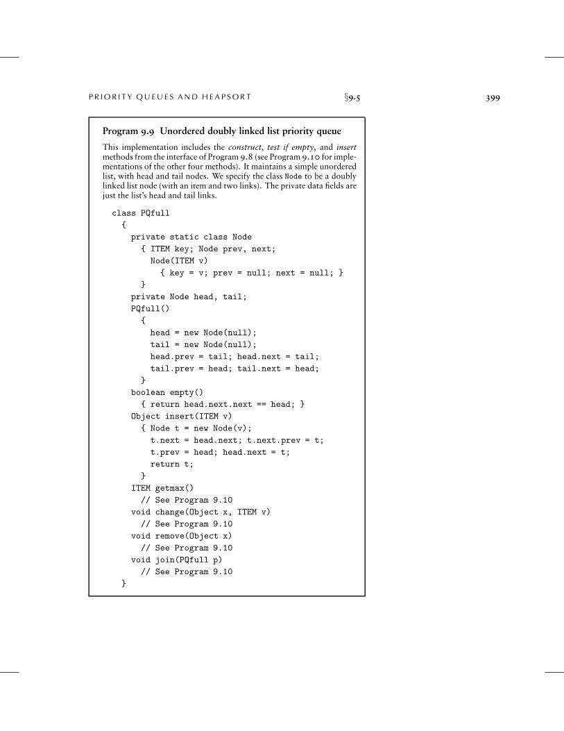
Program 9.9 Unordered doubly linked list priority queue

This implementation includes the construct, test if empty, and insertmethods from the interface of Program 9.8 (see Program 9.10 for imple-mentations of the other four methods). It maintains a simple unorderedlist, with head and tail nodes. We specify the class Node to be a doublylinked list node (with an item and two links). The private data fields arejust the list’s head and tail links.

class PQfull

{private static class Node

{ ITEM key; Node prev, next;

Node(ITEM v)

{ key = v; prev = null; next = null; }

}

private Node head, tail;

PQfull()

{

head = new Node(null);

tail = new Node(null);

head.prev = tail; head.next = tail;

tail.prev = head; tail.next = head;

}

boolean empty(){ return head.next.next == head; }

Object insert(ITEM v)

{ Node t = new Node(v);

t.next = head.next; t.next.prev = t;

t.prev = head; head.next = t;

return t;

}

ITEM getmax()

// See Program 9.10

void change(Object x, ITEM v)

// See Program 9.10

void remove(Object x)

// See Program 9.10

void join(PQfull p)// See Program 9.10

}

400 §9.5 C H A P T E R N I N E

copy semantics come into play. We are not considering the copyoperation and have chosen just one out of several possibilities for join(see Exercises 9.44 and 9.45).

It is easy to add such procedures to the interface in Program 9.8,but it is much more challenging to develop an implementation wherelogarithmic performance for all operations is guaranteed. In applica-tions where the priority queue does not grow to be large, or where themix of insert and remove the maximum operations has some specialproperties, a fully flexible interface might be desirable. But in applica-tions where the queue will grow to be large, and where a tenfold or ahundredfold increase in performance might be noticed or appreciated,it might be worthwhile to restrict to the set of operations where effi-cient performance is assured. A great deal of research has gone into thedesign of priority-queue algorithms for different mixes of operations;the binomial queue described in Section 9.7 is an important example.

Exercises

9.39 Which priority-queue implementation would you use to find the 100smallest of a set of 106 random numbers? Justify your answer.

9.40 Provide implementations similar to Programs 9.9 and 9.10 that useordered doubly linked lists. Note: Because the client has handles into the datastructure, your programs can change only links (rather than keys) in nodes.

9.41 Provide implementations for insert and remove the maximum (thepriority-queue interface in Program 9.1) using complete heap-ordered treesrepresented with explicit nodes and links. Note: Because the client has nohandles into the data structure, you can take advantage of the fact that it iseasier to exchange information fields in nodes than to exchange the nodesthemselves.

• 9.42 Provide implementations for insert, remove the maximum, change pri-ority, and remove (the priority-queue interface in Program 9.8) using heap-ordered trees with explicit links. Note: Because the client has handles intothe data structure, this exercise is more difficult than Exercise 9.41, not justbecause the nodes have to be triply linked, but also because your programscan change only links (rather than keys) in nodes.

9.43 Add a (brute-force) implementation of the join operation to your im-plementation from Exercise 9.42.

◦9.44 Suppose that we add a clone method to Program 9.8 (and specify thatevery implementation implements Cloneable). Add an implementation ofclone to Programs 9.9 and 9.10, and write a driver program that tests yourinterface and implementation.


Program 9.10 Doubly linked list priority queue (continued)

These method implementations complete the priority queue implemen-tation of Program 9.9. The remove the maximum operation requiresscanning through the whole list, but the overhead of maintaining doublylinked lists is justified by the fact that the change priority, remove, andjoin operations all are implemented in constant time, using only elemen-tary operations on the lists (see Chapter 3 for more details on doublylinked lists).

The change and remove methods take an Object reference as aparameter, which must reference an object of (private) type Node—aclient can only get such a reference from insert.

We might make this class Cloneable and implement a clonemethod that makes a copy of the whole list (see Section 4.9), but clientobject handles would be invalid for the copy. The join implementationappropriates the list nodes from the parameter to be included in theresult, but it does not make copies of them, so client handles remainvalid.

ITEM getmax()

{ ITEM max; Node x = head.next;

for (Node t = x; t.next != head; t = t.next)

if (Sort.less(x.key, t.key)) x = t;

max = x.key;

remove(x);

return max;

}

void change(Object x, ITEM v)

{ ((Node) x).key = v; }

void remove(Object x)

{ Node t = (Node) x;

t.next.prev = t.prev;t.prev.next = t.next;

}

void join(PQfull p)

{

tail.prev.next = p.head.next;

p.head.next.prev = tail.prev;

head.prev = p.tail;

p.tail.next = head;

tail = p.tail;

}

402 §9.6 C H A P T E R N I N E

• 9.45 Change the interface and implementation for the join operation in Pro-grams 9.9 and 9.10 such that it returns a PQfull (the result of joining theparameters).

9.46 Provide a priority-queue interface and implementation that supportsconstruct and remove the maximum, using tournaments (see Section 5.7).Program 5.19 will provide you with the basis for construct.

• 9.47 Add insert to your solution to Exercise 9.46.

9.6 Priority Queues for Client Arrays

Suppose that the records to be processed in a priority queue are in anexisting array. In this case, it makes sense to have the priority-queueroutines refer to items through the array index. Moreover, we can usethe array index as a handle to implement all the priority-queue oper-ations. An interface along these lines is illustrated in Program 9.11.Figure 9.13 shows how this approach might apply for a small example.Without copying or making special modifications of records, we cankeep a priority queue containing a subset of the records.

Using indices into an existing array is a natural arrangement, butit leads to implementations with an orientation opposite to that ofProgram 9.8. Now it is the client program that cannot move aroundinformation freely, because the priority-queue routine is maintainingindices into data maintained by the client. For its part, the priorityqueue implementation must not use indices without first being giventhem by the client.

To develop an implementation, we use precisely the same ap-proach as we did for index sorting in Section 6.8. We manipulateindices and define less such that comparisons reference the client’sarray. There are added complications here, because the priority-queueroutine must keep track of the objects so that it can find them when theclient program refers to them by the handle (array index). To this end,we add a second index array to keep track of the position of the keys inthe priority queue. To localize the maintenance of this array, we movedata only with the exch operation and define exch appropriately.

Program 9.12 is a heap-based implementation of this approachthat differs only slightly from Program 9.5 but is well worth studyingbecause it is so useful in practice. We refer to the data structure builtby this program as an index heap. We shall use this program as a


90

87 84

86 86

Figure 9.13Index heap data structures

k qp[k] pq[k] data[k]

0 Wilson 631 5 3 Johnson 862 2 2 Jones 873 1 4 Smith 904 3 9 Washington 845 1 Thompson 656 Brown 827 Jackson 618 White 769 4 Adams 8610 Black 71

By manipulating indices, ratherthan the records themselves, wecan build a priority queue on asubset of the records in an array.Here, a heap of size 5 in the arraypq contains the indices to thosestudents with the top five grades.Thus, data[pq[1]].name con-tains Smith, the name of the stu-dent with the highest grade, andso forth. An inverse array qp al-lows the priority-queue routines totreat the array indices as handles.For example, if we need to changeSmith’s grade to 85, we changethe entry in data[3].grade, thencall PQchange(3). The priority-queue implementation accessesthe record at pq[qp[3]] (orpq[1], because qp[3]=1) and thenew key at data[pq[1]].name(or data[3].name, becausepq[1]=3).

Program 9.11 Priority-queue ADT interface for index items

Instead of building a data structure from the items themselves, thisinterface provides for building a priority queue using indices into aclient array. The constructor takes a reference to an array as a param-eter, and the insert, remove the maximum, change priority, and removemethods all use indices into that array and compare array entries withITEM’s less method. For example, the client program might defineless so that less(i, j) is the result of comparing data[i].grade anddata[j].grade.

class PQi // ADT interface

{ // implementations and private members hiddenPQi(Array)

boolean empty()

void insert(int)

int getmax()

void change(int)

void remove(int)

};

building block for other algorithms in Parts 5 through 7. As usual,we do no error checking, and we assume (for example) that indicesare always in the proper range and that the user does not try to insertanything on a full queue or to remove anything from an empty one.Adding code for such checks is straightforward.

We can use the same approach for any priority queue that uses anarray representation (for example, see Exercises 9.50 and 9.51). Themain disadvantage of using indirection in this way is the extra spaceused. The size of the index arrays has to be the size of the data array,when the maximum size of the priority queue could be much less.

Other approaches to building a priority queue on top of existingdata in an array are either to have the client program make recordsconsisting of a key with its array index as associated information orto use a class for index keys with its own less method. Then, ifthe implementation uses a linked-allocation representation such as theone in Programs 9.9 and 9.10 or Exercise 9.42, then the space usedby the priority queue would be proportional to the maximum numberof elements on the queue at any one time. Such approaches would

404 §9.6 C H A P T E R N I N E

Program 9.12 Index-heap–based priority queue

This implementation of Program 9.11 maintains pq as an array of in-dices into a client array.

We keep the heap position corresponding to index value kin qp[k], which allows us to implement change priority (see Fig-ure 9.14) and remove (see Exercise 9.49). We maintain the invariantpq[qp[k]]=qp[pq[k]]=k for all k in the heap (see Figure 9.13). Themethods less and exch are the key to the implementation—they allowus to use the same sink and swim code as for standard heaps.

class PQi

{

private boolean less(int i, int j)

{ return a[pq[i]].less(pq[j]); }

private void exch(int i, int j)

{ int t = pq[i]; pq[i] = pq[j]; pq[j] = t;

qp[pq[i]] = i; qp[pq[j]] = j;}


// Program 9.3


// Program 9.4

private ITEM[] a;

private int[] pq, qp;

private int N;

PQi(ITEM[] items)

{ a = items; N = 0;

pq = new int[a.length+1];

qp = new int[a.length+1];

}

boolean empty(){ return N == 0; }

void insert(int v)

{ pq[++N] = v; qp[v] = N; swim(N); }

int getmax()

{ exch(1, N); sink(1, N-1); return pq[N--]; }

void change(int k)

{ swim(qp[k]); sink(qp[k], N); }

};


X

S P

G R O N

A E B A I M

YX P

G S O N

A E R A I M

X

P

G S O N

A E R A I M

Figure 9.14Changing of the priority of

a node in a heapThe top diagram depicts a heapthat is heap-ordered, except possi-bly at one given node. If the nodeis larger than its parent, then itmust move up, just as depictedin Figure 9.3. This situation is il-lustrated in the middle diagram,with Y moving up the tree (in gen-eral, it might stop before hittingthe root). If the node is smallerthan the larger of its two children,then it must move down, just asdepicted in Figure 9.4. This situ-ation is illustrated in the bottomdiagram, with B moving down thetree (in general, it might stop be-fore hitting the bottom). We canuse this procedure in two ways:as the basis for the change prior-ity operation on heaps in order toreestablish the heap condition afterchanging the key in a node, or asthe basis for the remove operationon heaps in order to reestablish theheap condition after replacing thekey in a node with the rightmostkey on the bottom level.

be preferred over Program 9.12 if space must be conserved and if thepriority queue involves only a small fraction of the data array.

Contrasting this approach to providing a complete priority-queueimplementation to the approach in Section 9.5 exposes essential dif-ferences in ADT design. In the first case (Programs 9.9 and 9.10, forexample), it is the responsibility of the priority-queue implementationto allocate and deallocate the memory for the keys, to change keyvalues, and so forth. The ADT supplies the client with handles toitems, and the client accesses items only through calls to the priority-queue routines, using the handles as parameters. In the second case(Program 9.12, for example), the client is responsible for the keysand records, and the priority-queue routines access this informationonly through handles provided by the user (array indices, in the caseof Program 9.12). Both uses require cooperation between client andimplementation.

Note that, in this book, we are normally interested in coop-eration beyond that encouraged by programming language supportmechanisms. In particular, we want the performance characteristics ofthe implementation to match the dynamic mix of operations requiredby the client. One way to ensure that match is to seek implementationswith provable worst-case performance bounds, but we can solve manyproblems more easily by matching their performance requirementswith simpler implementations.

Exercises

9.48 Suppose that an array is filled with the keys E A S Y Q U E S T I O N.Give the contents of the pq and qp arrays after these keys are inserted into aninitially empty heap using Program 9.12.

◦9.49 Add a remove operation to Program 9.12.

9.50 Implement the priority-queue ADT for index items (see Program 9.11)using an ordered-array representation for the priority queue.

9.51 Implement the priority-queue ADT for index items (see Program 9.11)using an unordered-array representation for the priority queue.

◦9.52 Given an array a of N elements, consider a complete binary tree of 2Nelements (represented as an array pq) containing indices from the array with thefollowing properties: (i) for i from 0 to N-1, we have pq[N+i]=i; and (ii) fori from 1 to N-1, we have pq[i]=pq[2*i] if a[pq[2*i]]>a[pq[2*i+1]], andwe have pq[i]=pq[2*i+1] otherwise. Such a structure is called an index heaptournament because it combines the features of index heaps and tournaments

406 §9.7 C H A P T E R N I N E

(see Program 5.19). Give the index heap tournament corresponding to thekeys E A S Y Q U E S T I O N.

◦9.53 Implement the priority-queue ADT for index items (see Program 9.11)using an index heap tournament (see Exercise 9.46).

9.7 Binomial Queues

None of the implementations that we have considered admit implemen-tations of join, remove the maximum, and insert that are all efficientin the worst case. Unordered linked lists have fast join and insert, butslow remove the maximum; ordered linked lists have fast remove themaximum, but slow join and insert; heaps have fast insert and removethe maximum, but slow join; and so forth. (See Table 9.1.) In applica-tions where frequent or large join operations play an important role,we need to consider more advanced data structures.

In this context, we mean by “efficient” that the operations shoulduse no more than logarithmic time in the worst case. This restrictionwould seem to rule out array representations, because we can jointwo large arrays apparently only by moving all the elements in atleast one of them. The unordered doubly linked-list representation ofProgram 9.9 does the join in constant time but requires that we walkthrough the whole list for remove the maximum. Use of a doublylinked ordered list (see Exercise 9.40) gives a constant-time remove themaximum but requires linear time to merge lists for join.

Numerous data structures have been developed that can supportefficient implementations of all the priority-queue operations. Mostof them are based on direct linked representation of heap-orderedtrees. Two links are needed for moving down the tree (either to bothchildren in a binary tree or to the first child and next sibling in abinary tree representation of a general tree), and one link to the parentis needed for moving up the tree. Developing implementations ofthe heap-ordering operations that work for any (heap-ordered) treeshape with explicit nodes and links or other representation is generallystraightforward. The difficulty lies in dynamic operations such asinsert, remove, and join, which require us to modify the tree structure.Different data structures are based on different strategies for modifyingthe tree structure while still maintaining balance in the tree. Thealgorithms use trees that are both more flexible than are complete


T

S N

R

O

A G

I

W

P

L

E

E

T

S

R N

O A G I

W

P

L E

E

Figure 9.15A binomial queue of size 13A binomial queue of size N is alist of left-heap-ordered power-of-2 heaps, one for each bit in thebinary representation of N . Thus,a binomial queue of size 13 =11012 consists of an 8-heap, a 4-heap, and a 1-heap. Shown hereare the left-heap-ordered power-of-2 heap representation (top) andthe heap-ordered binomial-treerepresentation (bottom) of the samebinomial queue.

trees and keep the trees sufficiently balanced to ensure a logarithmictime bound.

The overhead of maintaining a triply linked structure—ensuringthat a particular implementation correctly maintains three pointers inall circumstances—can be burdensome (see Exercise 9.41). Moreover,in many practical situations, it is difficult to demonstrate that effi-cient implementations of all the operations are required, so we mightpause before taking on such an implementation. On the other hand, itis also difficult to demonstrate that efficient implementations are notrequired, and the investment to guarantee that all the priority-queueoperations will be fast may be justified. Regardless of such consid-erations, the next step from heaps to a data structure that allows forefficient implementation of join, insert, and remove the maximum isfascinating and worthy of study in its own right.

Even with a linked representation for the trees, the heap conditionand the condition that the heap-ordered binary tree be complete aretoo strong to allow efficient implementation of the join operation.Given two heap-ordered trees, how do we merge them together intojust one tree? For example, if one of the trees has 1023 nodes andthe other has 255 nodes, how can we merge them into a tree with1278 nodes, without touching more than 10 or 20 nodes? It seemsimpossible to merge heap-ordered trees in general if the trees are tobe heap ordered and complete, but various advanced data structureshave been devised that weaken the heap-order and balance conditionsto get the flexibility that we need to devise an efficient join. Next,we consider an ingenious solution to this problem, called the binomialqueue, that was developed by Vuillemin in 1978.

To begin, we note that the join operation is trivial for one partic-ular type of tree with a relaxed heap-ordering restriction.

Definition 9.4 A binary tree comprising nodes with keys is said tobe left-heap-ordered if the key in each node is larger than or equal toall the keys in that node’s left subtree (if any).

Definition 9.5 A power-of-2 heap is a left-heap-ordered tree consist-ing of a root node with an empty right subtree and a complete leftsubtree. The tree corresponding to a power-of-2 heap by the left-child,right-sibling correspondence is called a binomial tree.

408 §9.7 C H A P T E R N I N E

XT

S WR N P M

O A G I L E A E

XW

P M

L E A E

TS

R N

O A G I

X

T W

S

R

O

A

N

G

I P

L

E

M

A

E

XW

P

M

L

E A

E

TS

R

N

O

A G

I

Figure 9.16Joining of two equal-sized

power-of-2 heaps.We join two power-of-two heaps(top) by putting the larger of theroots at the root, with that root’s(left) subtree as the right subtreeof the other original root. If theoperands have 2n nodes, the resulthas 2n+1 nodes. If the operandsare left-heap-ordered, then so isthe result, with the largest keyat the root. The heap-orderedbinomial-tree representation of thesame operation is shown below theline.

Program 9.13 Joining of two equal-sized power-of-2 heaps

We need to change only a few links to combine two equal-sized power-of-2 heaps into one power-of-2 heap that is twice that size. This method,which we define as a private method in the implementation, is one keyto the efficiency of the binomial queue algorithm.

static Node pair(Node p, Node q)

{

if (p.item.less(q.item))

{ p.r = q.l; q.l = p; return q; }

else { q.r = p.l; p.l = q; return p; }

}

Binomial trees and power-of-2 heaps are equivalent. We workwith both representations because binomial trees are slightly easierto visualize, whereas the simple representation of power-of-2 heapsleads to simpler implementations. In particular, we depend upon thefollowing facts, which are direct consequences of the definitions:• The number of nodes in a power-of-2 heap is a power of 2.• No node has a key larger than the key at the root.• Binomial trees are heap-ordered.

The trivial operation upon which binomial-queue algorithms arebased is that of joining two power-of-2 heaps that have an equal num-ber of nodes. The result is a heap with twice as many nodes which iseasy to create, as illustrated in Figure 9.16. The root node with thelarger key becomes the root of the result (with the other original rootas the result root’s left child), with its left subtree becoming the rightsubtree of the other root node. Given a linked representation for thetrees, the join is a constant-time operation: We simply adjust two linksat the top. An implementation is given in Program 9.13. This basicoperation is at the heart of Vuillemin’s general solution to the problemof implementing priority queues with no slow operations.

Definition 9.6 A binomial queue is a set of power-of-2 heaps, notwo of the same size. The structure of a binomial queue is determinedby that queue’s number of nodes, by correspondence with the binaryrepresentation of integers.


A binomial queue of N elements has one power-of-2 heap foreach 1 bit in the binary representation of N . For example, a binomialqueue of 13 nodes comprises an 8-heap, a 4-heap, and a 1-heap, asillustrated in Figure 9.15. There are at most lgN power-of-2 heaps ina binomial queue of size N , all of height no greater than lgN .

In accordance with Definitions 9.5 and 9.6, we represent power-of-2 heaps (and handles to items) as links to nodes containing keys andtwo links (like the explicit tree representation of tournaments in Fig-ure 5.10); and we represent binomial queues as arrays of power-of-2heaps, by including the following private members in our implemen-tation of Program 9.8:

private static class Node

{ ITEM item; Node l, r;

Node(ITEM v)

{ item = v; l = null; r = null; }

}

private Node[] bq;

The arrays are not large and the trees are not high; and this rep-resentation is sufficiently flexible to allow implementation of all thepriority-queue operations in less than lgN steps, as we shall now see.

Each link in the array bq is a link to a power-of-2 heap: bq[i] iseither null or a link to a 2i-heap. As the queue grows and shrinks, thelength of the array increases and decreases, but much less frequently:for example, the array length increases by 1 only after the queue sizedoubles. It will be convenient to always have the last link null, so webegin with an array of size 1, a null link:

PQfull()

{ bq = new Node[1]; bq[0] = null; }

thus adopting the convention that a queue is empty if and only if thearray is of length 1.

Now, let us consider the insert operation. The process of insert-ing a new item into a binomial queue mirrors precisely the processof incrementing a binary number. To increment a binary number, wemove from right to left, changing 1s to 0s because of the carry associ-ated with 1 + 1 = 102, until finding the rightmost 0, which we changeto 1. In the analogous way, to add a new item to a binomial queue, wemove from right to left, merging heaps corresponding to 1 bits with a

410 §9.7 C H A P T E R N I N E

WT

N P

E I L E

W

P

L E

T

I

E

N

TN

E I

NE

Figure 9.17Insertion of a new element

into a binomial queueAdding an element to a binomialqueue of 7 nodes is analogousto performing the binary addition1112 + 1 = 10002, with carries ateach bit. The result is the binomialqueue at the bottom, with an 8-heap and null 4-, 2-, and 1-heaps.

Program 9.14 Insertion into a binomial queue

To insert a node into a binomial queue, we first make the node into a 1-heap, identify it as a carry 1-heap, and then iterate the following processstarting at i = 0. If the binomial queue has no 2i-heap, we put the carry2i-heap into the queue. If the binomial queue has a 2i-heap, we combinethat with the new one (using the pair method from Program 9.13) tomake a 2i+1-heap, increment i, and iterate until finding an empty heapposition in the binomial queue. When we carry in to the null link at theend of the array, we call grow to increase the size of the array by 1 andput a null link in the new position (see text).

Object insert(ITEM v)

{ Node t = new Node(v), c = t;

for (int i = 0; i < bq.length+1; i++){

if (c == null) break;

if (i == bq.length-1) bq = grow(bq);

if (bq[i] == null) { bq[i] = c; break; }

c = pair(c, bq[i]); bq[i] = null;

}

return t;

}

carry heap, until finding the rightmost empty position to put the carryheap.

Specifically, to insert a new item into a binomial queue, we makethe new item into a 1-heap. Then, ifN is even (rightmost bit 0), we justput this 1-heap in the empty rightmost position of the binomial queue.If N is odd (rightmost bit 1), we join the 1-heap corresponding to thenew item with the 1-heap in the rightmost position of the binomialqueue to make a carry 2-heap. If the position corresponding to 2 inthe binomial queue is empty, we put the carry heap there; otherwise,we merge the carry 2-heap with the 2-heap from the binomial queue tomake a carry 4-heap, and so forth, continuing until we get to an emptyposition in the binomial queue. This process is depicted in Figure 9.17;Program 9.14 is an implementation.

When we add an element to a binomial queue with 2k − 1 itemsto make one with 2k items, we carry into the null link at the end ofthe array, replacing it with a binomial tree of size 2k (the rest of the


TS

R N

O A G I

WP

L E

MA

E

XT

S WR N P M

O A G I L E A E

Figure 9.18Removal of the maximum in a

power-of-2 heapTaking away the root gives a forestof power-of-2 heaps, all left-heapordered, with roots from the rightspine of the tree. This operationleads to a way to remove the max-imum element from a binomialqueue: Take away the root of thepower-of-2 heap that contains thelargest element, then use the joinoperation to merge the resultingbinomial queue with remainingpower-of-2 heaps in the originalbinomial queue.

Program 9.15 Removal of the maximum in a binomial queue

We first scan the root nodes to find the maximum and remove thepower-of-2 heap containing the maximum from the binomial queue.We then remove the root node containing the maximum from its power-of-2 heap and temporarily build a binomial queue that contains theremaining constituent parts of the power-of-2 heap. Finally, we usethe join operation to merge this binomial queue back into the originalbinomial queue.

ITEM getmax()

{ int i, max; ITEM v = null;

for (i = 0, max = -1; i < bq.length; i++)

if (bq[i] != null)

if ((max == -1) || v.less(bq[i].item))

{ max = i; v = bq[max].item; }

Node[] temp = new Node[max+1]; temp[max] = null;

Node x = bq[max].l; bq[max] = null;

for (i = max-1; i >= 0; i--){ temp[i] = x; x = x.r; temp[i].r = null; }

bq = BQjoin(bq, temp);

return v;

}

links are all null). To adhere to our convention in this case, we needto add a null link at the end, which necessitates increasing the size ofthe array by 1. The method grow that Program 9.14 invokes for thistask is simple to implement (see Exercise 9.62).

Other binomial-queue operations are also best understood byanalogy with binary arithmetic. As we shall see, implementing joincorresponds to implementing addition for binary numbers.

For the moment, assume that we have an (efficient) method forjoin that is organized to merge the priority-queue reference in its secondoperand with the priority-queue reference in its first operand (leavingthe result in the first operand). Using this method, we could implementthe insert operation with a call to the join method where one of theoperands is a binomial queue of size 1 (see Exercise 9.66).

We can also implement the remove the maximum operation withone call to join. To find the maximum item in a binomial queue, we

412 §9.7 C H A P T E R N I N E

TS

R N

O A G I

WP

L E

MA

E

W

P

L E

E

TS

R N

O A G I

MA

Figure 9.19Joining of two binomial

queues (no carry)When two binomial queues to bejoined do not have any power-of-2 heaps of the same size, thejoin operation is a simple merge.Doing this operation is analo-gous to adding two binary num-bers without ever encountering1 + 1 (no carry). Here, a bino-mial queue of 10 nodes is mergedwith one of 5 nodes to make oneof 15 nodes, corresponding to10102 + 01012 = 11112 .

scan the queue’s power-of-2 heaps. Each of these heaps is left-heap-ordered, so it has its maximum element at the root. The largest of theitems in the roots is the largest element in the binomial queue. Becausethere are no more than lgN heaps in the binomial queue, the totaltime to find the maximum element is less than lgN .

To perform the remove the maximum operation, we note thatremoving the root of a left-ordered 2k-heap leaves k left-ordered power-of-2 heaps—a 2k−1-heap, a 2k−2-heap, and so forth—which we caneasily restructure into a binomial queue of size 2k − 1, as illustratedin Figure 9.18. Then, we can use the join operation to combine thisbinomial queue with the rest of the original queue in order to completethe remove the maximum operation. This implementation is given inProgram 9.15.

How do we join two binomial queues? First, we note that theoperation is trivial if they do not contain two power-of-2 heaps of thesame size, as illustrated in Figure 9.19: we simply merge the heapsfrom the two binomial queues to make one binomial queue. A queueof size 10 (consisting of an 8-heap and a 2-heap) and a queue ofsize 5 (consisting of a 4-heap and a 1-heap) simply merge together tomake a queue of size 15 (consisting of an 8-heap, a 4-heap, a 2-heap,and a 1-heap). The more general case follows by direct analogy withperforming addition on two binary numbers, complete with carry, asillustrated in Figure 9.20.

For example, when we add a queue of size 7 (consisting of a4-heap, a 2-heap, and a 1-heap) to a queue of size 3 (consisting ofa 2-heap and a 1-heap), we get a queue of size 10 (consisting of an8-heap and a 2-heap); to do the addition, we need to merge the 1-heaps and carry a 2-heap, then merge the 2-heaps and carry a 4-heap,then merge the 4-heaps to get an 8-heap result, in a manner preciselyanalogous to the binary addition 0112 + 1112 = 10102. The exampleof Figure 9.19 is simpler than Figure 9.20 because it is analogous to10102 + 01012 = 11112, with no carry.

This direct analogy with binary arithmetic carries through to giveus a natural implementation for the join operation (see Program 9.16).For each bit, there are eight cases to consider, based on all the pos-sible different values for the 3 bits involved (carry and 2 bits in theoperands). The code is more complicated than that for plain addition,because we are dealing with distinguishable heaps, rather than with


WT

N P

E I L E

M

A

W

P

L E

M

A

E

T

I

N

TN

E I

NE

Figure 9.20Joining of two binomial

queuesAdding a binomial queue of 3nodes to one of 7 nodes gives oneof 10 nodes through a processthat mimics the binary addition0112 + 1112 = 10102 . Adding N toE gives an empty 1-heap in the re-sult with a carry 2-heap containingN and E. Then, adding the three2-heaps leaves a 2-heap in the re-sult with a carry 4-heap containingT N E I. This 4-heap is added tothe other 4-heap, producing the bi-nomial queue at the bottom. Fewnodes are touched in the process.

indistinguishable bits, but each case is straightforward. For example,if all 3 bits are 1, we need to leave a heap in the result binomial queueand to join the other two heaps for the carry into the next position.Indeed, this operation brings us full cycle on abstract data types: we(barely) resist the temptation to cast Program 9.16 as a purely abstractbinary addition procedure, with the binomial-queue implementationnothing more than a client program using the more complicated bitaddition procedure in Program 9.13.

We do a join operation after reducing the size of the binomialqueue by 1. If the next-to-last link in the result is null, then we canshrink the size of the array by 1, since the last link in the result will benull. The method shrink that Program 9.16 invokes for this task issimple to implement (see Exercise 9.62).

Property 9.7 All the operations for the priority-queue ADT can beimplemented with binomial queues such that O(lgN) steps are re-quired for any operations performed on an N -item queue.

These performance bounds are the goal of the design of the data struc-ture. They are direct consequences of the fact that the implementationsall have only one or two loops that iterate through the roots of thetrees in the binomial queue.

Another option, which leads to a slightly simpler implementa-tion, is to keep the number of trees in the queue constant (see Exer-cise 9.64) so that the running time of all the methods is proportionalto this number (the logarithm of the maximum size of the binomialqueue).

Property 9.8 Construction of a binomial queue with N insert oper-ations on an initially empty queue requires O(N) comparisons in theworst case.

For one-half the insertions (when the queue size is even and there isno 1-heap), no comparisons are required; for one-half the remaininginsertions (when there is no 2-heap), only 1 comparison is required;when there is no 4-heap, only 2 comparisons are required; and soforth. Thus, the total number of comparisons is less than 0 ·N/2 + 1 ·N/4 + 2 ·N/8 + . . . < N .

Binomial queues provide guaranteed fast performance, but datastructures have been designed with even better theoretical performance

414 §9.7 C H A P T E R N I N E

Program 9.16 Joining (merging) of two binomial queues

This code mimics the operation of adding two binary numbers. Pro-ceeding from right to left with an initial carry bit of 0, we treat theeight possible cases (all possible values of the operands and carry bits)in a straightforward manner. For example, case 3 corresponds to theoperand bits being both 1 and the carry 0. Then, the result is 0, but thecarry is 1 (the result of adding the operand bits).

We exchange the references if necessary to make a reference thequeue with the larger array representation, and we increase or decreasethe size of a’s array for the result, if warranted. If there is a carry intothe last (null) link in case 4, it invokes grow; if the next-to-last link isnull after the operation is complete, it invokes shrink.

Like pair, this method is a private method in the implementation,which is called by getmax and join. The implementation of the ADTmethod join(PQfull p) is the invocation BQjoin(bq, p.bq).

static int bit(Node x){ return x == null ? 0 : 1; }

static int bits(Node C, Node B, Node A)

{ return 4*bit(C) + 2*bit(B) + 1*bit(A); }

static Node[] BQjoin(Node[] a, Node[] b)

{ Node c = null;

if (a.length < b.length)

{ Node[] t = a; a = b; b = t; }

for (int i = 0; i < b.length; i++)

switch(bits(c, b[i], a[i]))

{

case 2: a[i] = b[i]; break;

case 3: c = pair(a[i], b[i]);

a[i] = null; break;

case 4: if (i == a.length-1) a = grow(a);a[i] = c; c = null; break;

case 5: c = pair(c, a[i]);

a[i] = null; break;

case 6:

case 7: c = pair(c, b[i]); break;

}

if (a[a.length-1] == null) a = shrink(a);

return a;

}


characteristics, providing guaranteed constant-time performance forcertain operations. This problem is an interesting and active area ofdata-structure design. On the other hand, the practical utility of manyof these esoteric structures is dubious. Before delving into complexdata-structure solutions, we need to be certain that performance bot-tlenecks exist that we can relieve only by reducing the running time ofsome priority-queue operation. Indeed, for practical applications, weshould prefer a trivial structure for debugging and for small queues;then, we should use heaps to speed up the operations unless fast joinoperations are required; finally, we should use binomial queues toguarantee logarithmic performance for all operations. All things con-sidered, however, a priority-queue package based on binomial queuesis a valuable addition to a software library.

Exercises.9.54 Draw a binomial queue of size 29, using the binomial-tree representa-

tion.

• 9.55 Write a program to draw the binomial-tree representation of a binomialqueue, given the size N (just nodes connected by edges, no keys).

9.56 Give the binomial queue that results when the keys E A S Y Q U E S T IO N are inserted into an initially empty binomial queue.

9.57 Give the binomial queue that results when the keys E A S Y are insertedinto an initially empty binomial queue, and give the binomial queue that resultswhen the keys Q U E S T I O N are inserted into an initially empty binomialqueue. Then give the result of remove the maximum for each queue. Finally,give the result when the join operation is performed on the resulting queues.

9.58 Using the conventions of Exercise 9.1, give the sequence of binomialqueues produced when the operations

P R I O * R * * I * T * Y * * * Q U E * * * U * E

are performed on an initially empty binomial queue.

9.59 Using the conventions of Exercise 9.2, give the sequence of binomialqueues produced when the operations

( ( ( P R I O *) + ( R * I T * Y * ) ) * * * ) + ( Q U E * * * U * E )

are performed on an initially empty binomial queue.

9.60 Prove that a binomial tree with 2n nodes has(ni

)nodes at level i for

0 ≤ i ≤ n. (This fact is the origin of the name binomial tree.)

.9.61 Give an implementation for empty() that is appropriate for thebinomial-queue implementation given in the text.

416 §9.7 C H A P T E R N I N E

9.62 Implement the grow and shrink methods that increase by one anddecrease by one, respectively, the size of a Node array leaving a null link in thelast array position (shrink should throw an exception if that is not the case).

9.63 Change the binomial-queue implementation in the text to represent thequeues with Java Vector objects instead of arrays.

◦9.64 Develop a binomial-queue implementation that uses a fixed-size arrayof representation so that grow and shrink are not needed, but the operationsall take time proportional to the array size.

◦9.65 Modify your solution such that Property 9.7 holds, by maintaining asentinel pointer to mark the point where the loops should terminate.

• 9.66 Implement insert for binomial queues by just using the join operationexplicitly.

•• 9.67 Implement change priority and remove for binomial queues. Note: Youwill need to add a third link, which points up the tree, to the nodes.

• 9.68 Add an implementation of clone to the binomial-queue implementa-tions (Programs 9.13 through 9.16) in the text, and test your implementationwith your driver program from Exercise 9.44.

• 9.69 Empirically compare binomial queues against heaps as the basis forsorting, as in Program 9.6, for randomly ordered keys with N = 1000, 104,105, and 106.

• 9.70 Develop an in-place sorting method like heapsort, but based on bino-mial queues. Hint: See Exercise 9.38.

Documents

Priority Queues and Heapsort MANY APPLICATIONS REQUIRE ... · Priority Queues and Heapsort MANY APPLICATIONS REQUIRE that we process records with keys in order, but not necessarily