Prior vs Likelihood vs Posterior Posterior Predictive ... vs Likelihood vs Posterior Posterior Predictive Distribution Poisson Data ... e.g. Normal vs tdf † Probability of events

Prior vs Likelihood vs PosteriorPosterior Predictive Distribution

Poisson Data

Statistics 220

Spring 2005

Copyright c©2005 by Mark E. Irwin

Choosing the Likelihood Model

While much thought is put into thinking about priors in a Bayesian Analysis,the data (likelihood) model can have a big effect.

Choices that need to be made involve

• Independence vs Exchangable vs More Complex Dependence

• Tail size, e.g. Normal vs tdf

• Probability of events

Choosing the Likelihood Model 1

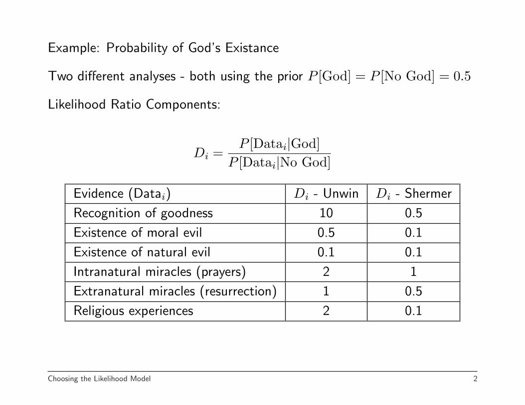
Example: Probability of God’s Existance

Two different analyses - both using the prior P [God] = P [No God] = 0.5

Likelihood Ratio Components:

Di =P [Datai|God]

P [Datai|No God]

Evidence (Datai) Di - Unwin Di - Shermer

Recognition of goodness 10 0.5

Existence of moral evil 0.5 0.1

Existence of natural evil 0.1 0.1

Intranatural miracles (prayers) 2 1

Extranatural miracles (resurrection) 1 0.5

Religious experiences 2 0.1


P [God|Data]:

• Unwin: 23

• Shermer: 0.00025

So even starting with the same prior, the difference beliefs about what thedata says gives quite different posterior probabilities.

This is based on an analysis published in an July 2004 Scientific Americanarticle. (Available on the course web site on the Articles page.)

Stephen D. Unwin is a risk management consultant who has done work inphysics on quantum gravity. He is author of the book The Probability ofGod.

Michael Shermer is the publisher of Skeptic and a regular contributor toScientific American as author of the column Skeptic.


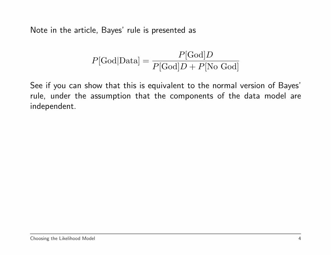
Note in the article, Bayes’ rule is presented as

P [God|Data] =P [God]D

P [God]D + P [No God]

See if you can show that this is equivalent to the normal version of Bayes’rule, under the assumption that the components of the data model areindependent.


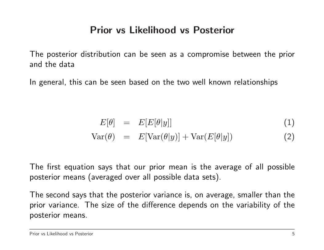
Prior vs Likelihood vs Posterior

The posterior distribution can be seen as a compromise between the priorand the data

In general, this can be seen based on the two well known relationships

E[θ] = E[E[θ|y]] (1)

Var(θ) = E[Var(θ|y)] + Var(E[θ|y]) (2)

The first equation says that our prior mean is the average of all possibleposterior means (averaged over all possible data sets).

The second says that the posterior variance is, on average, smaller than theprior variance. The size of the difference depends on the variability of theposterior means.

Prior vs Likelihood vs Posterior 5

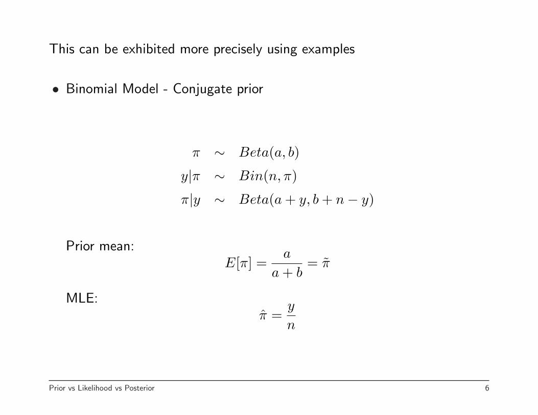
This can be exhibited more precisely using examples

• Binomial Model - Conjugate prior

π ∼ Beta(a, b)

y|π ∼ Bin(n, π)

π|y ∼ Beta(a + y, b + n− y)

Prior mean:E[π] =

a

a + b= π

MLE:π =

y

n


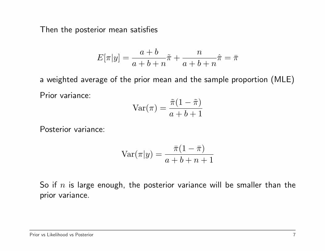
Then the posterior mean satisfies

E[π|y] =a + b

a + b + nπ +

n

a + b + nπ = π

a weighted average of the prior mean and the sample proportion (MLE)

Prior variance:

Var(π) =π(1− π)a + b + 1

Posterior variance:

Var(π|y) =π(1− π)

a + b + n + 1

So if n is large enough, the posterior variance will be smaller than theprior variance.


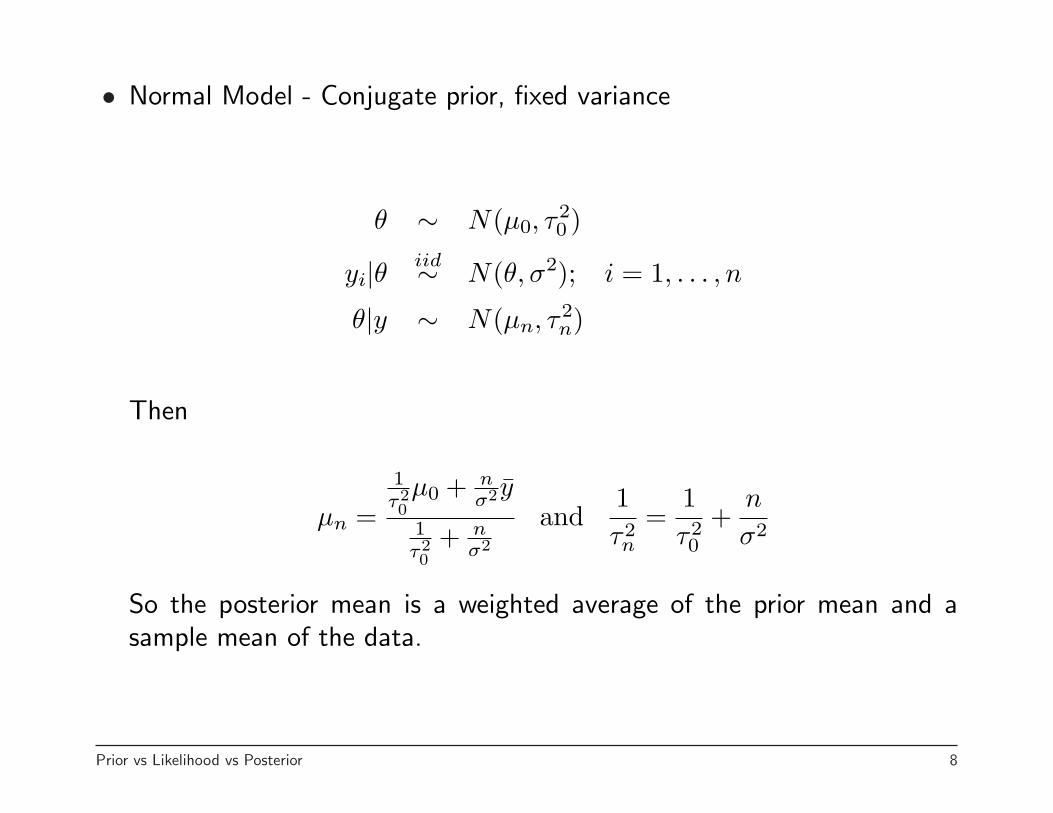
• Normal Model - Conjugate prior, fixed variance

θ ∼ N(µ0, τ20 )

yi|θ iid∼ N(θ, σ2); i = 1, . . . , n

θ|y ∼ N(µn, τ2n)

Then

µn =1τ20µ0 + n

σ2 y

1τ20

+ nσ2

and1τ2n

=1τ20

+n

σ2

So the posterior mean is a weighted average of the prior mean and asample mean of the data.


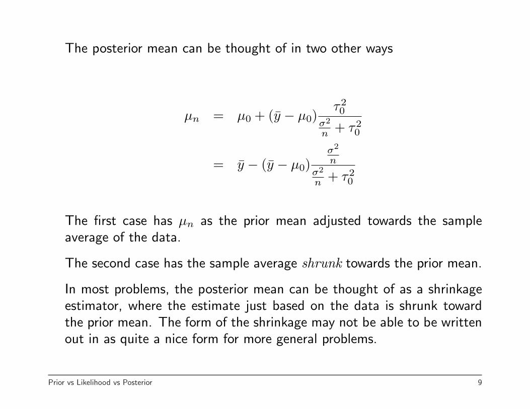
The posterior mean can be thought of in two other ways

µn = µ0 + (y − µ0)τ20

σ2

n + τ20

= y − (y − µ0)σ2

nσ2

n + τ20

The first case has µn as the prior mean adjusted towards the sampleaverage of the data.

The second case has the sample average shrunk towards the prior mean.

In most problems, the posterior mean can be thought of as a shrinkageestimator, where the estimate just based on the data is shrunk towardthe prior mean. The form of the shrinkage may not be able to be writtenout in as quite a nice form for more general problems.


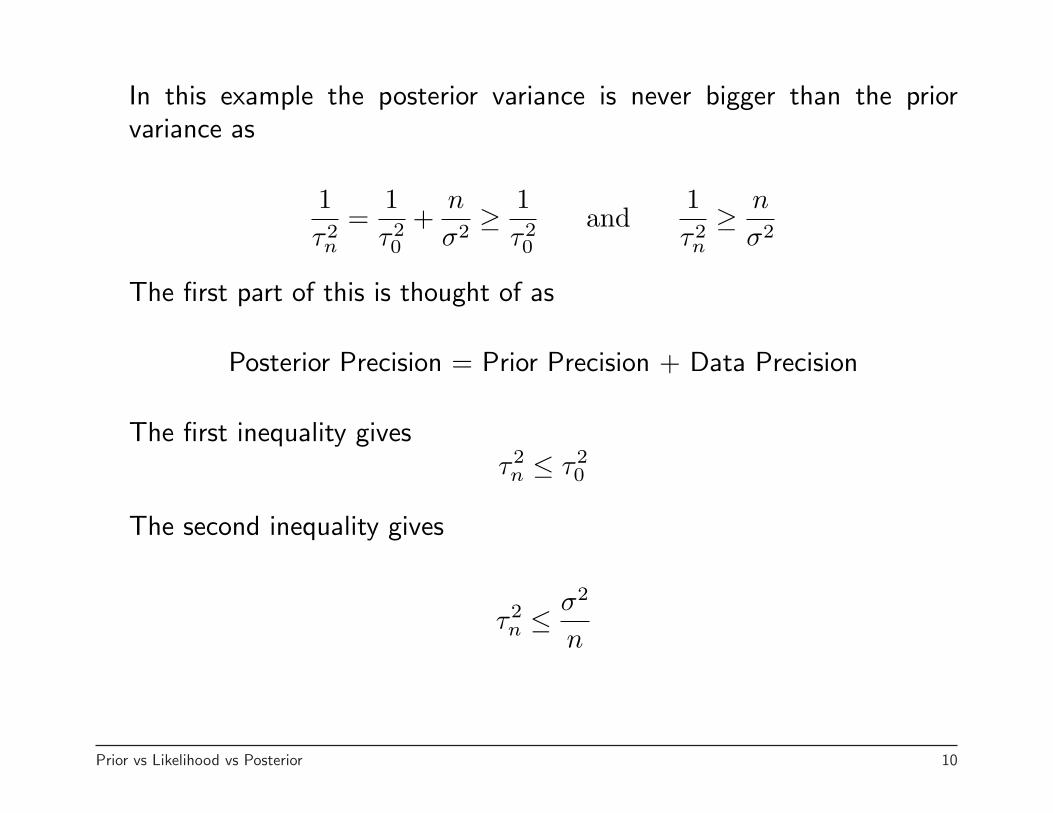
In this example the posterior variance is never bigger than the priorvariance as

1τ2n

=1τ20

+n

σ2≥ 1

τ20

and1τ2n

≥ n

σ2

The first part of this is thought of as

Posterior Precision = Prior Precision + Data Precision

The first inequality givesτ2n ≤ τ2

0

The second inequality gives

τ2n ≤

σ2

n


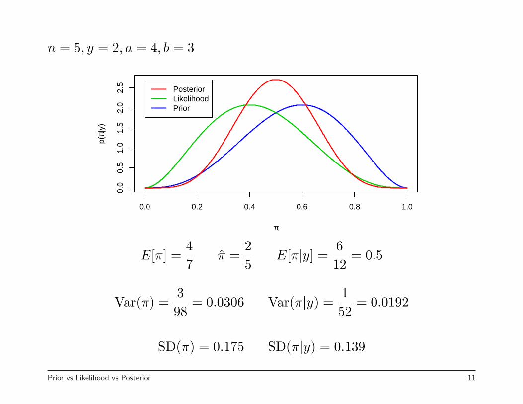
n = 5, y = 2, a = 4, b = 3

0.0 0.2 0.4 0.6 0.8 1.0

0.0

0.5

1.0

1.5

2.0

2.5

π

p(π|

y)

PosteriorLikelihoodPrior

E[π] =47

π =25

E[π|y] =612

= 0.5

Var(π) =398

= 0.0306 Var(π|y) =152

= 0.0192

SD(π) = 0.175 SD(π|y) = 0.139


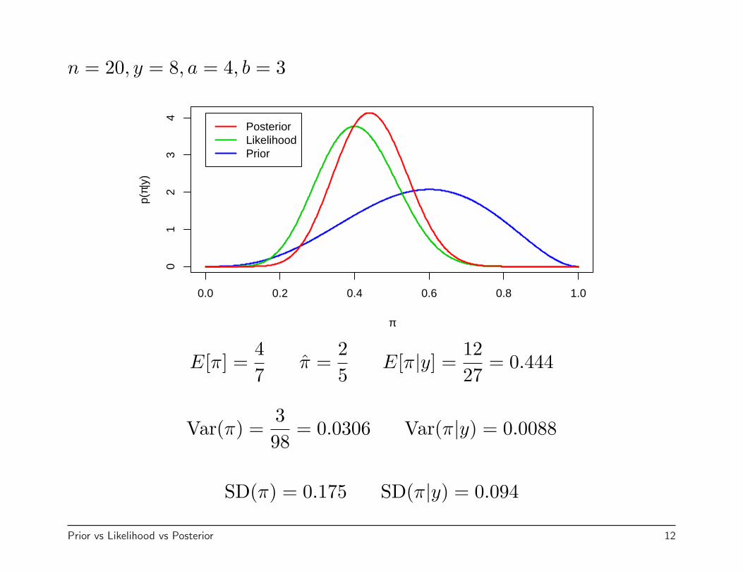
n = 20, y = 8, a = 4, b = 3

0.0 0.2 0.4 0.6 0.8 1.0

01

23

4

π

p(π|

y)


E[π] =47

π =25

E[π|y] =1227

= 0.444

Var(π) =398

= 0.0306 Var(π|y) = 0.0088

SD(π) = 0.175 SD(π|y) = 0.094


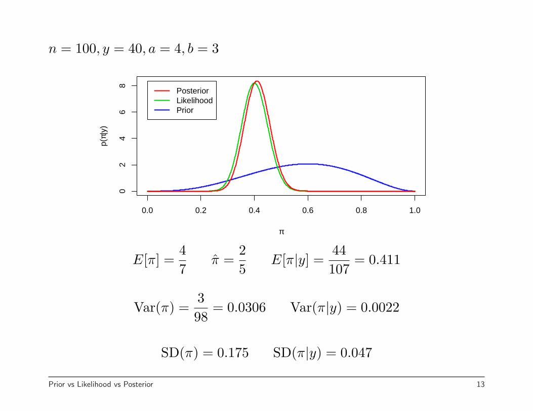
n = 100, y = 40, a = 4, b = 3

0.0 0.2 0.4 0.6 0.8 1.0

02

46

8

π

p(π|

y)


E[π] =47

π =25

E[π|y] =44107

= 0.411

Var(π) =398

= 0.0306 Var(π|y) = 0.0022

SD(π) = 0.175 SD(π|y) = 0.047


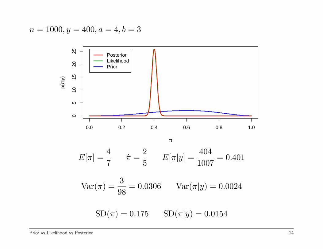
n = 1000, y = 400, a = 4, b = 3

0.0 0.2 0.4 0.6 0.8 1.0

05

1015

2025

π

p(π|

y)


E[π] =47

π =25

E[π|y] =4041007

= 0.401

Var(π) =398

= 0.0306 Var(π|y) = 0.0024

SD(π) = 0.175 SD(π|y) = 0.0154


Prediction

Another useful summary is the posterior predictive distribution of a futureobservation, y

p(y|y) =∫

p(y|y, θ)p(θ|y)dθ

In many situations, y will be conditionally independent of y given θ. Thusthe distribution in this case reduces to

p(y|y) =∫

p(y|θ)p(θ|y)dθ

In many situations this can be difficult to calculate, though it is often easywith a conjugate prior.

Prediction 15

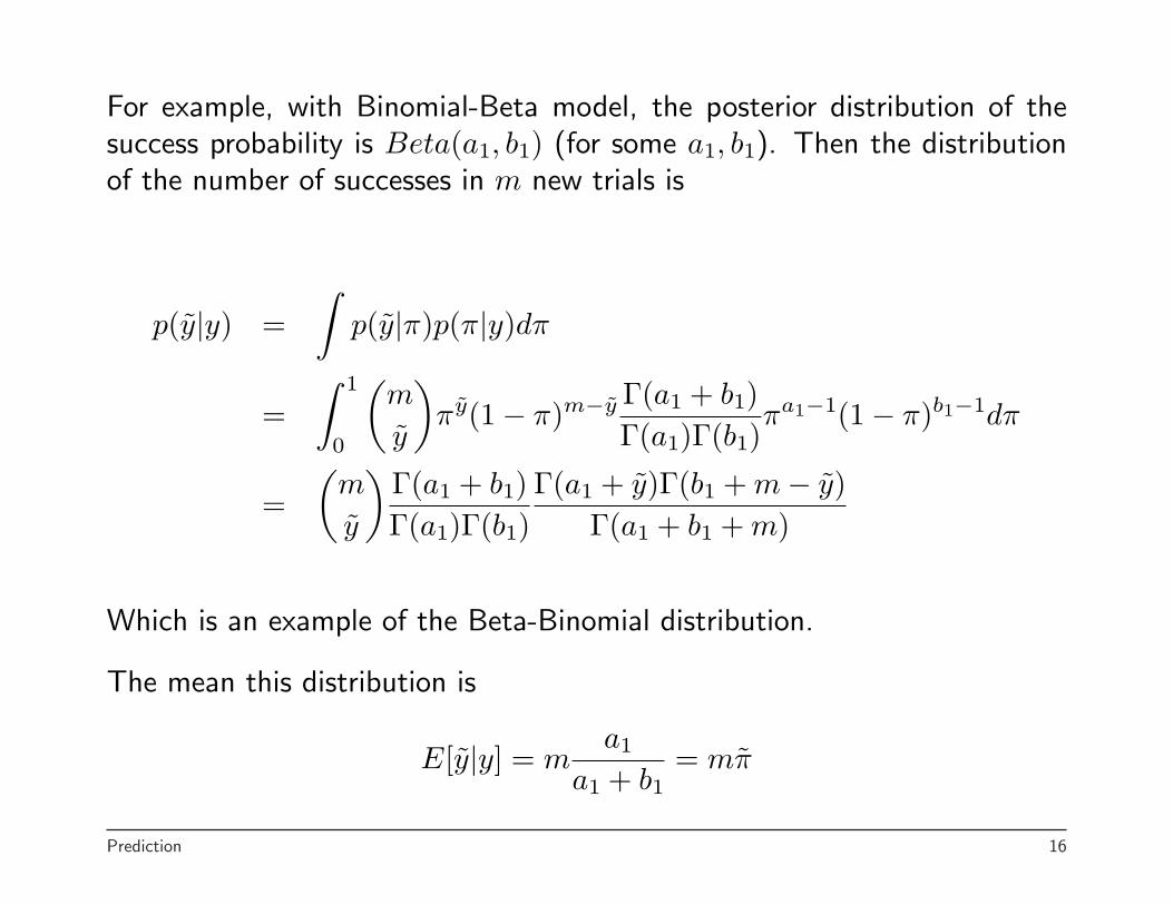
For example, with Binomial-Beta model, the posterior distribution of thesuccess probability is Beta(a1, b1) (for some a1, b1). Then the distributionof the number of successes in m new trials is

p(y|y) =∫

p(y|π)p(π|y)dπ

=∫ 1

0

(m

y

)πy(1− π)m−y Γ(a1 + b1)

Γ(a1)Γ(b1)πa1−1(1− π)b1−1dπ

=(

m

y

)Γ(a1 + b1)Γ(a1)Γ(b1)

Γ(a1 + y)Γ(b1 + m− y)Γ(a1 + b1 + m)

Which is an example of the Beta-Binomial distribution.

The mean this distribution is

E[y|y] = ma1

a1 + b1= mπ

Prediction 16

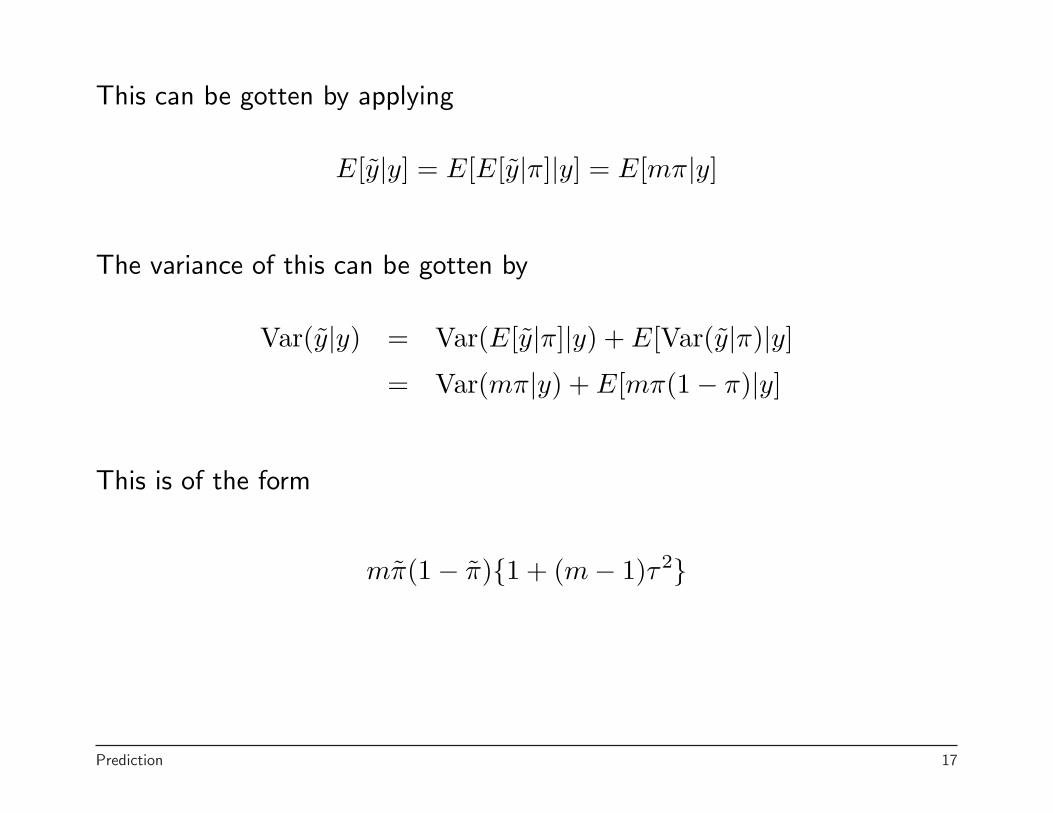
This can be gotten by applying

E[y|y] = E[E[y|π]|y] = E[mπ|y]

The variance of this can be gotten by

Var(y|y) = Var(E[y|π]|y) + E[Var(y|π)|y]

= Var(mπ|y) + E[mπ(1− π)|y]

This is of the form

mπ(1− π){1 + (m− 1)τ2}

Prediction 17

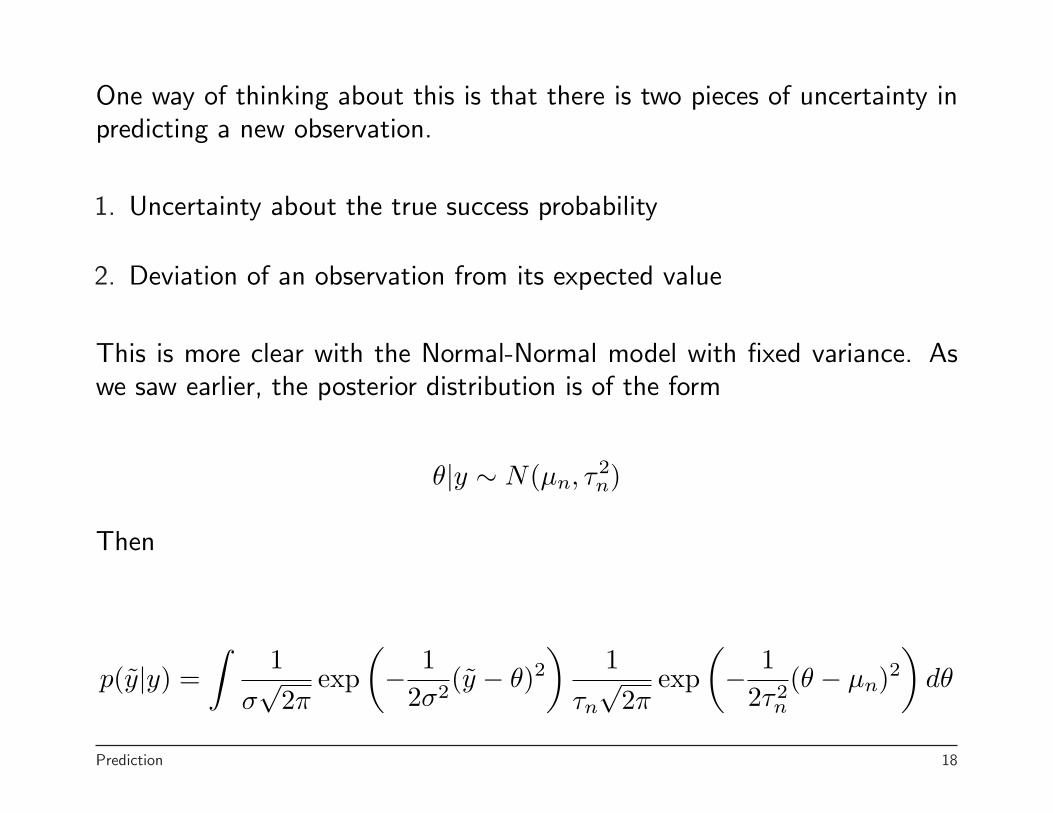
One way of thinking about this is that there is two pieces of uncertainty inpredicting a new observation.

1. Uncertainty about the true success probability

2. Deviation of an observation from its expected value

This is more clear with the Normal-Normal model with fixed variance. Aswe saw earlier, the posterior distribution is of the form

θ|y ∼ N(µn, τ2n)

Then

p(y|y) =∫

1σ√

2πexp

(− 1

2σ2(y − θ)2

)1

τn

√2π

exp(− 1

2τ2n

(θ − µn)2)

dθ

Prediction 18

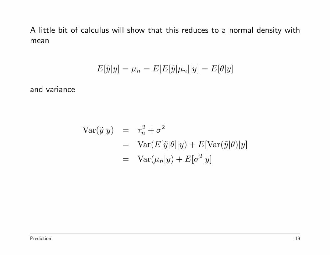
A little bit of calculus will show that this reduces to a normal density withmean

E[y|y] = µn = E[E[y|µn]|y] = E[θ|y]

and variance

Var(y|y) = τ2n + σ2

= Var(E[y|θ]|y) + E[Var(y|θ)|y]

= Var(µn|y) + E[σ2|y]

Prediction 19

An analogue to this is the variance for prediction in linear regression. It isexactly of this form

Var(y|x) = σ2

(1 +

1n

+(x− x)2

(n− 1)s2x

)

Simulating the posterior predictive distribution

This is easy to do, assuming that you can simulate from the posteriordistribution of the parameter, which is usually feasible.

To do it involves two steps:

1. Simulate θi from θ|y; i = 1, . . . , m

2. Simulate yi from y|θi (= y|θi, y); i = 1, . . . , m

The pairs (θi, yi) are draws from the joint distribution θ, y|y. Therefore theyi are draws from y|y.

Prediction 20

Why interest in the posterior predictive distribution?

• You might want to do predictions. For example, what will happen to astock in 6 months.

• Model checking: Is your model reasonable?

There are a number of ways of doing this. Future observations could becompared with the posterior predictive distribution.

Another option might be something along the lines of cross validation. Fitthe model with part of the data and compare the remaining observationto the posterior predictive distribution calculated from the sample usedfor fitting.

Prediction 21

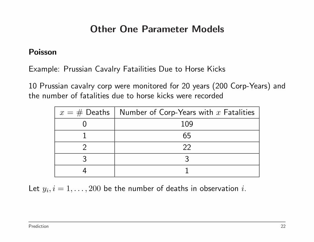
Other One Parameter Models

Poisson

Example: Prussian Cavalry Fatailities Due to Horse Kicks

10 Prussian cavalry corp were monitored for 20 years (200 Corp-Years) andthe number of fatalities due to horse kicks were recorded

x = # Deaths Number of Corp-Years with x Fatalities

0 109

1 65

2 22

3 3

4 1

Let yi, i = 1, . . . , 200 be the number of deaths in observation i.

Prediction 22

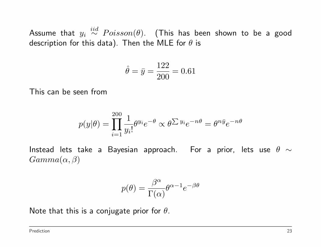
Assume that yiiid∼ Poisson(θ). (This has been shown to be a good

description for this data). Then the MLE for θ is

θ = y =122200

= 0.61

This can be seen from

p(y|θ) =200∏

i=1

1yi!

θyie−θ ∝ θP

yie−nθ = θnye−nθ

Instead lets take a Bayesian approach. For a prior, lets use θ ∼Gamma(α, β)

p(θ) =βα

Γ(α)θα−1e−βθ

Note that this is a conjugate prior for θ.

Prediction 23

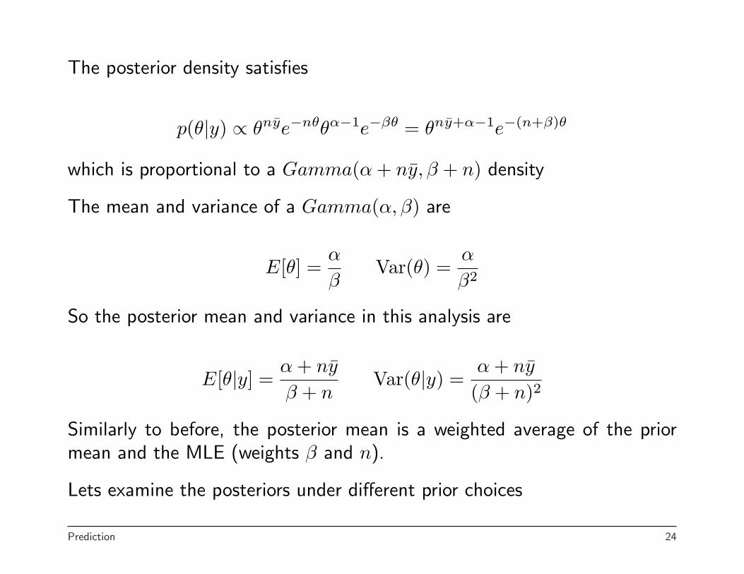
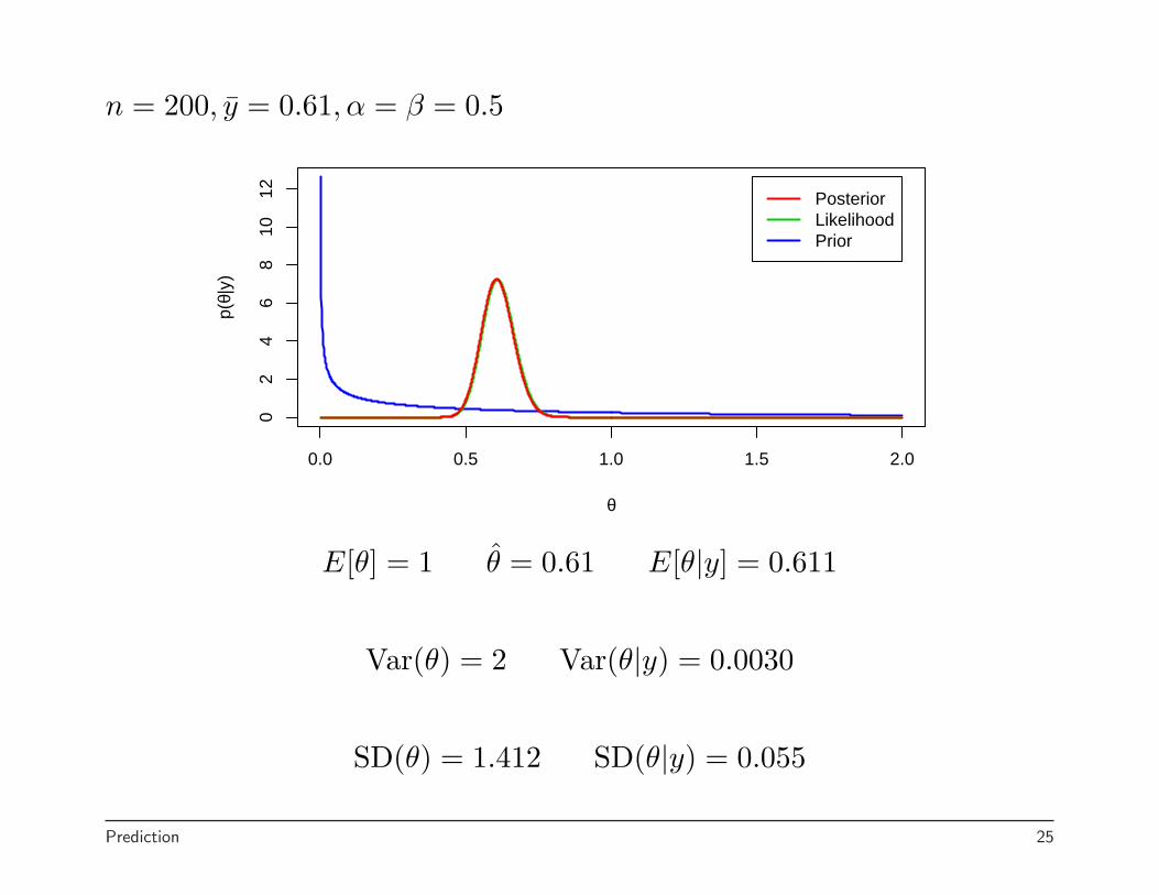
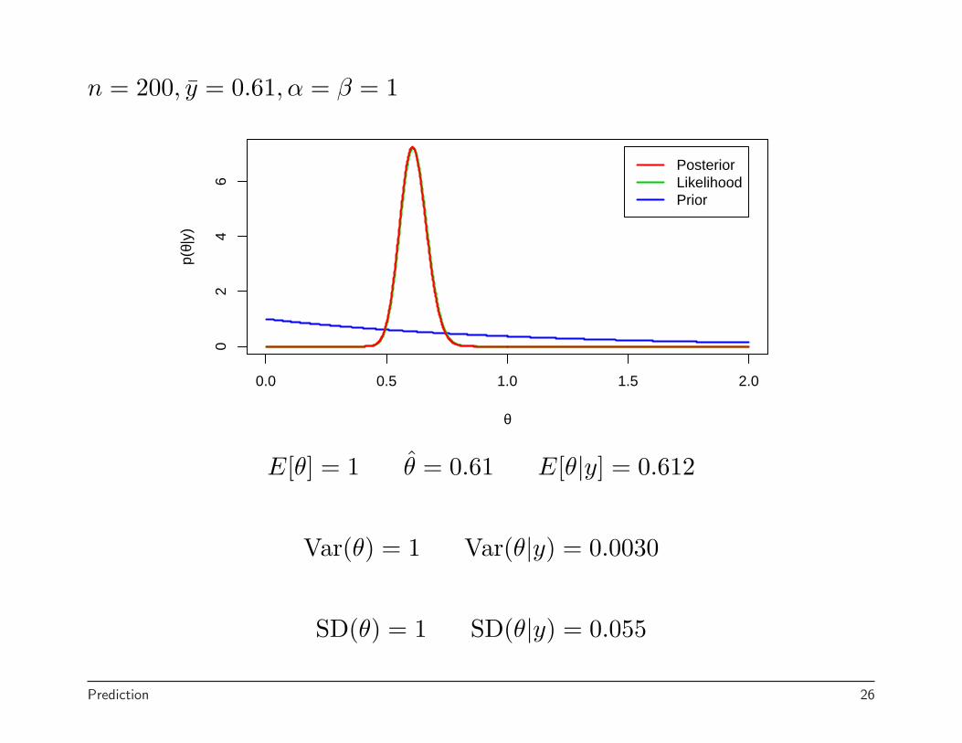
The posterior density satisfies

p(θ|y) ∝ θnye−nθθα−1e−βθ = θny+α−1e−(n+β)θ

which is proportional to a Gamma(α + ny, β + n) density

The mean and variance of a Gamma(α, β) are

E[θ] =α

βVar(θ) =

α

β2

So the posterior mean and variance in this analysis are

E[θ|y] =α + ny

β + nVar(θ|y) =

α + ny

(β + n)2

Similarly to before, the posterior mean is a weighted average of the priormean and the MLE (weights β and n).

Lets examine the posteriors under different prior choices

Prediction 24

n = 200, y = 0.61, α = β = 0.5

0.0 0.5 1.0 1.5 2.0

02

46

810

12

θ

p(θ|

y)PosteriorLikelihoodPrior

E[θ] = 1 θ = 0.61 E[θ|y] = 0.611

Var(θ) = 2 Var(θ|y) = 0.0030

SD(θ) = 1.412 SD(θ|y) = 0.055

Prediction 25

n = 200, y = 0.61, α = β = 1

0.0 0.5 1.0 1.5 2.0

02

46

θ

p(θ|


E[θ] = 1 θ = 0.61 E[θ|y] = 0.612

Var(θ) = 1 Var(θ|y) = 0.0030

SD(θ) = 1 SD(θ|y) = 0.055

Prediction 26

n = 200, y = 0.61, α = β = 10

0.0 0.5 1.0 1.5 2.0

02

46

θ

p(θ|


E[θ] = 1 θ = 0.61 E[θ|y] = 0.629

Var(θ) = 0.1 Var(θ|y) = 0.0030

SD(θ) = 0.316 SD(θ|y) = 0.055

Prediction 27

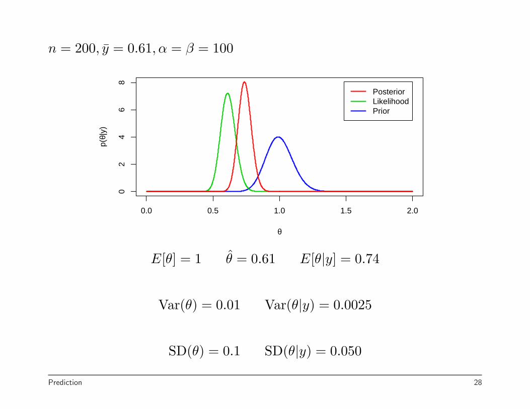
n = 200, y = 0.61, α = β = 100

0.0 0.5 1.0 1.5 2.0

02

46

8

θ

p(θ|


E[θ] = 1 θ = 0.61 E[θ|y] = 0.74

Var(θ) = 0.01 Var(θ|y) = 0.0025

SD(θ) = 0.1 SD(θ|y) = 0.050

Prediction 28

One way to think of the gamma prior in this case is that you have a dataset with β observations with and observed Poisson count of α.

Note that the Gamma distribution can be parameterized many ways.

Often the scale parameter form λ = 1β is used.

Also it can be parameterized in terms of mean, variance, and coefficient ofvariation (only two are needed).

This gives some flexibility in thinking about the desired form of the prior fora particular model.

In the example, I fixed the mean at 1 and let the variance decrease.

Prediction 29

Documents

Prior vs Likelihood vs Posterior Posterior Predictive ... vs Likelihood vs Posterior Posterior Predictive Distribution Poisson Data ... e.g. Normal vs tdf † Probability of events