Embed Size (px)
Citation preview

Princeton University
Ph410
Physics of Quantum Computation1
Kirk T. McDonald
(This version created July 13, 2017)
http://physics.princeton.edu/~mcdonald/examples/ph410problems.pdf
Reference: M.A. Nielsen and I.L. Chuang, Quantum Computation and Quantum Infor-mation (Cambridge UP, 2000)
See also the courses by Meglicki, Mermin and Preskill:
http://beige.ucs.indiana.edu/B679/
http://people.ccmr.cornell.edu/~mermin/qcomp/CS483.html
http://www.theory.caltech.edu/~preskill/
Copies of many papers relevant to this course are in the directoryhttp://physics.princeton.edu/~mcdonald/examples/QM/
in the format author journal vol page year.pdf
An electronic archive of unpublished papers on Quantum Physics (and many other topics)is at http://www.arxiv.org/
An electronic archive of published papers on Quantum Information is athttp://www.vjquantuminfo.org/quantuminfo/
1 A classic “quantum” computation: π = 3.1415 92653 58979... = “How I need a drink, alcoholic ofcourse, after the heavy lectures regarding quantum mechanics...” PC users, please change “alcoholic” to“cranberry” or “pineapple”. Skeptics can substitute “weirdness” for “mechanics”.
Problems
1. The Ultimate Laptop . . . . . . . . . . . . . . . . . . . . . . . . . . . . . . . . . . . . . . . . . . . . . . . . . . . . . . . . . . . . . 1
2. Maxwell’s Demon . . . . . . . . . . . . . . . . . . . . . . . . . . . . . . . . . . . . . . . . . . . . . . . . . . . . . . . . . . . . . . . . . 2
3. States, Bits and Unitary Operations . . . . . . . . . . . . . . . . . . . . . . . . . . . . . . . . . . . . . . . . . . . . . . . 8
4. Rotation Matrices . . . . . . . . . . . . . . . . . . . . . . . . . . . . . . . . . . . . . . . . . . . . . . . . . . . . . . . . . . . . . . . .15
5. Measurements . . . . . . . . . . . . . . . . . . . . . . . . . . . . . . . . . . . . . . . . . . . . . . . . . . . . . . . . . . . . . . . . . . . 21
6. Quantum Cloning and Quantum Teleportation . . . . . . . . . . . . . . . . . . . . . . . . . . . . . . . . . . . 28
7. Quantum Optics . . . . . . . . . . . . . . . . . . . . . . . . . . . . . . . . . . . . . . . . . . . . . . . . . . . . . . . . . . . . . . . . . 34
8. A Programmable Quantum Computer? . . . . . . . . . . . . . . . . . . . . . . . . . . . . . . . . . . . . . . . . . . 41
9. Designer Hamiltonians . . . . . . . . . . . . . . . . . . . . . . . . . . . . . . . . . . . . . . . . . . . . . . . . . . . . . . . . . . . 42
10. Deutsch’s Algorithm . . . . . . . . . . . . . . . . . . . . . . . . . . . . . . . . . . . . . . . . . . . . . . . . . . . . . . . . . . . . . 49
11. Universal Gates for Classical Computation . . . . . . . . . . . . . . . . . . . . . . . . . . . . . . . . . . . . . . . 54
12. Universal Gates for Quantum Computation . . . . . . . . . . . . . . . . . . . . . . . . . . . . . . . . . . . . . . 58
13. The Bernstein-Vazirani Problem . . . . . . . . . . . . . . . . . . . . . . . . . . . . . . . . . . . . . . . . . . . . . . . . . 65
14. Simon’s Problem . . . . . . . . . . . . . . . . . . . . . . . . . . . . . . . . . . . . . . . . . . . . . . . . . . . . . . . . . . . . . . . . . 67
15. Grover’s Search Algorithm . . . . . . . . . . . . . . . . . . . . . . . . . . . . . . . . . . . . . . . . . . . . . . . . . . . . . . . 69
16. Parity of a Function . . . . . . . . . . . . . . . . . . . . . . . . . . . . . . . . . . . . . . . . . . . . . . . . . . . . . . . . . . . . . .73
17. Quantum Fourier Transform, Shor’s Period-Finding Algorithm . . . . . . . . . . . . . . . . . . . 75
18. Nearest-Neighbor Algorithms . . . . . . . . . . . . . . . . . . . . . . . . . . . . . . . . . . . . . . . . . . . . . . . . . . . . .81
19. Spin Control . . . . . . . . . . . . . . . . . . . . . . . . . . . . . . . . . . . . . . . . . . . . . . . . . . . . . . . . . . . . . . . . . . . . . 86
20. Dephasing . . . . . . . . . . . . . . . . . . . . . . . . . . . . . . . . . . . . . . . . . . . . . . . . . . . . . . . . . . . . . . . . . . . . . . . 97
21. Quantum Error Correction . . . . . . . . . . . . . . . . . . . . . . . . . . . . . . . . . . . . . . . . . . . . . . . . . . . . . . 106
22. Fault-Tolerant Quantum Computation . . . . . . . . . . . . . . . . . . . . . . . . . . . . . . . . . . . . . . . . . . 113
23. Quantum Cryptography . . . . . . . . . . . . . . . . . . . . . . . . . . . . . . . . . . . . . . . . . . . . . . . . . . . . . . . . .120
24. The End of Quantum Information? . . . . . . . . . . . . . . . . . . . . . . . . . . . . . . . . . . . . . . . . . . . . . 125
i

Solutions
1. The Ultimate Laptop . . . . . . . . . . . . . . . . . . . . . . . . . . . . . . . . . . . . . . . . . . . . . . . . . . . . . . . . . . . 127
2. Maxwell’s Demon . . . . . . . . . . . . . . . . . . . . . . . . . . . . . . . . . . . . . . . . . . . . . . . . . . . . . . . . . . . . . . . 130
3. States, Bits and Unitary Operations . . . . . . . . . . . . . . . . . . . . . . . . . . . . . . . . . . . . . . . . . . . . 132
4. Rotation Matrices . . . . . . . . . . . . . . . . . . . . . . . . . . . . . . . . . . . . . . . . . . . . . . . . . . . . . . . . . . . . . . 140
5. Measurements . . . . . . . . . . . . . . . . . . . . . . . . . . . . . . . . . . . . . . . . . . . . . . . . . . . . . . . . . . . . . . . . . . 150
6. Quantum Cloning and Quantum Teleportation . . . . . . . . . . . . . . . . . . . . . . . . . . . . . . . . . . 155
7. Quantum Optics . . . . . . . . . . . . . . . . . . . . . . . . . . . . . . . . . . . . . . . . . . . . . . . . . . . . . . . . . . . . . . . . 165
8. A Programmable Quantum Computer? . . . . . . . . . . . . . . . . . . . . . . . . . . . . . . . . . . . . . . . . . 177
9. Designer Hamiltonians . . . . . . . . . . . . . . . . . . . . . . . . . . . . . . . . . . . . . . . . . . . . . . . . . . . . . . . . . . 178
10. Deutsch’s Algorithm . . . . . . . . . . . . . . . . . . . . . . . . . . . . . . . . . . . . . . . . . . . . . . . . . . . . . . . . . . . . 190
11. Universal Gates for Classical Computation . . . . . . . . . . . . . . . . . . . . . . . . . . . . . . . . . . . . . . 196
12. Universal Gates for Quantum Computation . . . . . . . . . . . . . . . . . . . . . . . . . . . . . . . . . . . . . 201
13. The Bernstein-Vazirani Problem . . . . . . . . . . . . . . . . . . . . . . . . . . . . . . . . . . . . . . . . . . . . . . . . 207
14. Simon’s Problem . . . . . . . . . . . . . . . . . . . . . . . . . . . . . . . . . . . . . . . . . . . . . . . . . . . . . . . . . . . . . . . . 211
15. Grover’s Search Algorithm . . . . . . . . . . . . . . . . . . . . . . . . . . . . . . . . . . . . . . . . . . . . . . . . . . . . . . 213
16. Parity of a Function . . . . . . . . . . . . . . . . . . . . . . . . . . . . . . . . . . . . . . . . . . . . . . . . . . . . . . . . . . . . 217
17. Quantum Fourier Transform, Shor’s Period-Finding Algorithm . . . . . . . . . . . . . . . . . . 218
18. Nearest-Neighbor Algorithms . . . . . . . . . . . . . . . . . . . . . . . . . . . . . . . . . . . . . . . . . . . . . . . . . . . 222
19. Spin Control . . . . . . . . . . . . . . . . . . . . . . . . . . . . . . . . . . . . . . . . . . . . . . . . . . . . . . . . . . . . . . . . . . . . 226
20. Dephasing . . . . . . . . . . . . . . . . . . . . . . . . . . . . . . . . . . . . . . . . . . . . . . . . . . . . . . . . . . . . . . . . . . . . . . 238
21. Quantum Error Correction . . . . . . . . . . . . . . . . . . . . . . . . . . . . . . . . . . . . . . . . . . . . . . . . . . . . . . 244
22. Fault-Tolerant Quantum Computation . . . . . . . . . . . . . . . . . . . . . . . . . . . . . . . . . . . . . . . . . . 248
23. Quantum Cryptography . . . . . . . . . . . . . . . . . . . . . . . . . . . . . . . . . . . . . . . . . . . . . . . . . . . . . . . . .251
i

Princeton University Ph410 Problem 1. The Ultimate Laptop 1
1. The Ultimate Laptop
A laptop computer weighs about 1 kg and occupies a volume of about 1 l.
Without knowing exactly what a quantum computer is, deduce limitations on the speed(N operations per second) and memory size (M in bits) of a laptop quantum computer,based on the uncertainty principle and thermodynamics/statistical mechanics.2 Howdoes the capability of the laptop depend on its temperature T ? Compare the operationof the laptop at room temperature to the case where all of the rest energy of the laptopis available.
It is instructive to relate the memory size of the laptop to its entropy.3
There might be some computational advantages to making the laptop as small aspossible. The ultimate compact laptop would be a 1-kg black hole. Given that theentropy of a black hole is roughly kA/L2
P , where k is Boltzmann’s constant, A is thesurface area, and LP is the Planck length, what is the memory size of the black-holelaptop?
“It from Bit” – John Archibald Wheeler
2If you feel the urge to “peek” at the literature, note that this problem is based onhttp://physics.princeton.edu/~mcdonald/examples/QM/bekenstein_prl_46_623_81.pdfSee also, http://physics.princeton.edu/~mcdonald/examples/QM/lloyd_nature_406_1047_00.pdf
3 For a high-level “reminder” about entropy (much more than needed here!), seehttp://physics.princeton.edu/~mcdonald/examples/QM/wehrl_rmp_50_221_78.pdf
Princeton University Ph410 Problem 2. Maxwell’s Demon 2
2. Maxwell’s Demon
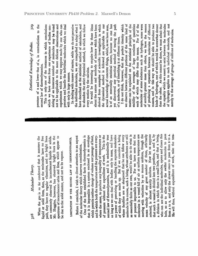
One of the earliest conceptual “supercomputers” was Maxwell’s Demon4, who uses in-telligence in sorting molecules to appear to evade the Second Law of Thermodynamics.
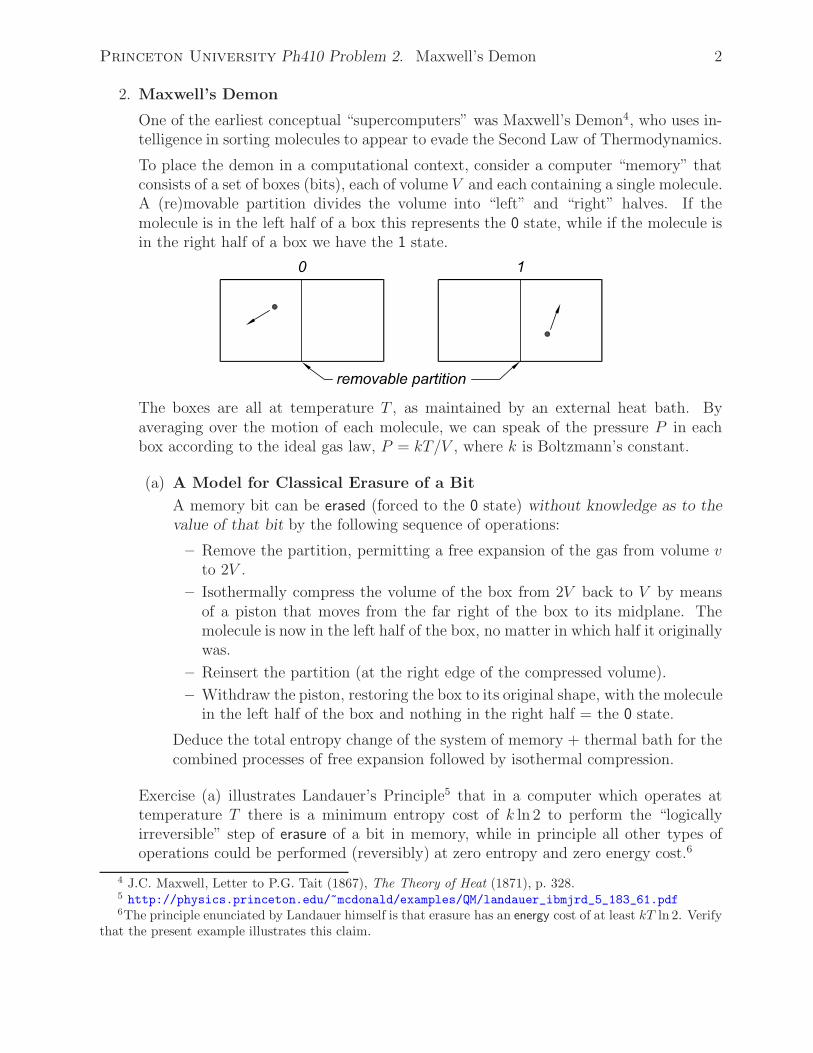
To place the demon in a computational context, consider a computer “memory” thatconsists of a set of boxes (bits), each of volume V and each containing a single molecule.A (re)movable partition divides the volume into “left” and “right” halves. If themolecule is in the left half of a box this represents the 0 state, while if the molecule isin the right half of a box we have the 1 state.
The boxes are all at temperature T , as maintained by an external heat bath. Byaveraging over the motion of each molecule, we can speak of the pressure P in eachbox according to the ideal gas law, P = kT/V , where k is Boltzmann’s constant.
(a) A Model for Classical Erasure of a Bit
A memory bit can be erased (forced to the 0 state) without knowledge as to thevalue of that bit by the following sequence of operations:
– Remove the partition, permitting a free expansion of the gas from volume vto 2V .
– Isothermally compress the volume of the box from 2V back to V by meansof a piston that moves from the far right of the box to its midplane. Themolecule is now in the left half of the box, no matter in which half it originallywas.
– Reinsert the partition (at the right edge of the compressed volume).
– Withdraw the piston, restoring the box to its original shape, with the moleculein the left half of the box and nothing in the right half = the 0 state.
Deduce the total entropy change of the system of memory + thermal bath for thecombined processes of free expansion followed by isothermal compression.
Exercise (a) illustrates Landauer’s Principle5 that in a computer which operates attemperature T there is a minimum entropy cost of k ln 2 to perform the “logicallyirreversible” step of erasure of a bit in memory, while in principle all other types ofoperations could be performed (reversibly) at zero entropy and zero energy cost.6
4 J.C. Maxwell, Letter to P.G. Tait (1867), The Theory of Heat (1871), p. 328.5 http://physics.princeton.edu/~mcdonald/examples/QM/landauer_ibmjrd_5_183_61.pdf6The principle enunciated by Landauer himself is that erasure has an energy cost of at least kT ln 2. Verify
that the present example illustrates this claim.

Princeton University Ph410 Problem 2. Maxwell’s Demon 3
An important extrapolation from Landauer’s Principle was made by Bennett7 whonoted that if a computer has a large enough memory such that no erasing need bedone during a computation, then the computation could be performed reversibly, andthe computer restored to its initial state at the end of the computation by undoing(reversing) the program once the answer was obtained.
The notion that computation could be performed by a reversible process was initiallyconsidered to be counterintuitive – and impractical. However, this idea was of greatconceptual importance because it opened the door to quantum computation, basedon quantum processes which are intrinsically reversible (except for measurement; seeprob. 5).
A second important distinction between classical and quantum computation (i.e.,physics), besides the irreversibility of quantum measurement, is that an arbitrary (un-known) quantum state cannot be copied exactly (prob. 6).
(b) Classical Copying of a Known Bit
In Bennett’s reversible computer there must be a mechanism for preserving theresult of a computation, before the computer is reversibly restored to its initialstate. Use the model of memory bits as boxes with a molecule in the left or righthalf to describe a (very simple) process whereby a bit, whose value is known, canbe copied at zero energy cost and zero entropy change onto a bit whose initialstate is 0.
A question left open by the previous discussion is whether the state of a classical bitcan be determined without an energy cost or entropy change.
In a computer, the way we show that we know the state of a bit is by making a copy ofit. To know the state of the bit, i.e., in which half of a memory box the molecule resides,we must make some kind of measurement. In principle, this can be done very slowlyand gently, by placing the box on a balance, or using the mechanical device sketchedon the following page,8 such that the energy cost is arbitrarily low, in exchange forthe measurement process being tedious, and the apparatus somewhat bulky. Thus,we accept the assertion of Bennett and Landauer that measurement and copying of aclassical bit are, in principle, cost-free operations.9
We can now contemplate another procedure for resetting a classical bit to 0. First,measure its state (making a copy in the process), and then subtract the copy from theoriginal. (We leave it as an optional exercise for you to concoct a procedure using themolecule in a box to implement the subtraction.) This appears to provide a scheme forerasure at zero energy/entropy cost, in contrast to the procedure you considered in part(a). However, at the end of the new procedure, the copy of the original bit remains,
7A thoughtful review by Bennett is athttp://physics.princeton.edu/~mcdonald/examples/QM/bennett_ibmjrd_32_16_88.pdfBennett’s original paper is athttp://physics.princeton.edu/~mcdonald/examples/QM/bennett_ibmjrd_17_525_73.pdf
8 http://physics.princeton.edu/~mcdonald/examples/QM/zurek_quant-ph-9807007.pdf9However, there is a kind of hidden entropy cost in the measurement process; namely the cost of preparing
in the 0 state the bits of memory where the results of the measurement can be stored.

Princeton University Ph410 Problem 2. Maxwell’s Demon 4
using up memory space. So to complete the erasure operation, we should also reset thecopy bit. This could be done at no energy/entropy cost by making yet another copy,and subtracting it from the first copy. To halt this silly cycle of resets, we must sooneror later revert to the procedure of part (a), which did not involve a measurement ofthe bit before resetting it. So, we must sooner or later pay the energy/entropy cost toerase a classical bit.
Recalling Maxwell’s demon, we see that his task of sorting molecules into the left half ofa partitioned box is equivalent to erasing a computer memory. The demon can performhis task with the aid of auxiliary equipment, which measures and stores informationabout the molecules. To finish his task cleanly, the demon must not only coax all themolecules into the left half of the box, but he must return his auxiliary equipmentto its original state (so that he could use it to sort a new set of molecules...poordemon). At some time during his task, the demon must perform a cleanup (erasure)operation equivalent to that of part (a), in which the entropy of the molecules/computerdecreases, but with an opposite and equal (or greater) increase in the entropy of theenvironment.
The demon obeys the Second Law of Thermodynamics10 – and performs his task mil-lions of times each second in your palm computer.
The “moral” of this problem is Landauer’s dictum:
Information is physical
.
10 For further reading, see chap. 5 of Feynman Lectures on Computation (Addison-Wesley, 1996),http://physics.princeton.edu/~mcdonald/examples/QM/bennett_ijtp_21_905_82.pdfhttp://physics.princeton.edu/~mcdonald/examples/QM/bennett_ibmjrd_32_16_88.pdfhttp://physics.princeton.edu/~mcdonald/examples/QM/bub_shpmp_32_569_01.pdf
Princeton University Ph410 Problem 2. Maxwell’s Demon 5

Princeton University Ph410 Problem 2. Maxwell’s Demon 6

Princeton University Ph410 Problem 2. Maxwell’s Demon 7

Princeton University Ph410 Problem 3. States, Bits and Unitary Operations 8
3. States, Bits and Unitary Operations
States and Bits. States of a system, or subsystem, involved in a computation willbe denoted in various equivalent ways. A Greek symbol such as ψ will sometimes beused. When considering a quantum system, we will often embed the symbol in a ket,following Dirac: |ψ〉. Our enthusiasm for this notation is such that we will often use itfor classical states as well.
We will deal almost exclusively with subsystems that have a finite number of inde-pendent (basis or eigen)states, in which case it is also useful to consider the state as avector. Thus, for a two-state system we write the state as a column vector:
ψ = |ψ〉 =
⎛⎝ ψ0
ψ1
⎞⎠ . (1)
If a classical system |ψ〉 has n states, it can be in only one of those states, say state|j〉. Then the vector components ψj of state |ψ〉,
|ψ〉 =∑j
ψj|j〉, (2)
have values ψj = 0 or 1.
A classical 2-state system could be used as a bit (or Cbit for classical bit) of a computermemory, and we define
|0〉 =
⎛⎝ 1
0
⎞⎠ , |1〉 =
⎛⎝ 0
1
⎞⎠ . (3)
An obvious mathematical generalization of a classical state is a vector in which thecomponents ψj are complex numbers (ψj = aj + ibj where aj and bj are real numbers,
and i =√−1 = eiπ/2). An ever-amazing physical fact is that quantum systems can be
well described by such vectors.
The physical meaning (as first explained by M. Born in 1927) of the complex vector
components of a quantum system is that the absolute square,∣∣∣ψj∣∣∣2, of a vector com-
ponent ψj is equal to the probability that the system will be found in state j IF ameasurement is made to determine the state of the system.
A measurement is a process that involves some kind of interaction of the quantumsystem with a more classical system such that the quantum system emerges with theclassical property of being in only one of its possible basis states. See prob. 5 for morediscussion of measurement.
An important distinction between a classical and a quantum state is that prior to ameasurement, a quantum state can be said to be in a superposition of several of itspossible basis states, while a classical system can only be in one basis state at time.This greater flexibility of quantum states compared to classical states is the core reasonwhy we might expect quantum computation, involving manipulation of quantum states,to offer greater opportunities than classical computation.
Princeton University Ph410 Problem 3. States, Bits and Unitary Operations 9
A physical restriction is that the total probability must be unity for finding a quantumsystem in some state. So we always assume the normalization condition,
|ψ|2 =∑j
∣∣∣ψj ∣∣∣2 = 1, (4)
for our quantum states (2). If we think of the state ψ as a (column) vector ψ as ineq. (1), then the normalization condition (4) could be written
ψ� ·ψ = 1, (5)
where the � implies complex conjugation. Anticipating the use of matrices along withthe state vectors, we can think of the vector ψ� in eq. (5) as a row vector,
ψ� = (ψ�0, ψ�1, . . . , ψ
�n). (6)
And, in the notation of Dirac, we introduce the bra of ψ as
ψ� = 〈ψ|. (7)
In sum, the various ways of writing the normalization condition for a quantum state are
|ψ|2 = 〈ψ|ψ〉 = ψ� ·ψ =∑j
∣∣∣ψj ∣∣∣2 = 1. (8)
Given two states |ψ〉 and |φ〉 we can define a vector dot product (inner product or scalarproduct) as
〈ψ|φ〉 = ψ� · φ =∑j
ψ�jφj. (9)
When 〈ψ|φ〉 = 0 we say that states |ψ〉 and |φ〉 are orthogonal.
The simplest quantum system of interest for computation is a 2-state system, whichcould function as a quantum bit (or Qbit). The zero and one states can be written as ineq. (3), and a general Qbit can be written as in eq. (1), together with the normalizationcondition that
|ψ0|2 + |ψ1|2 = 1. (10)
The general Qbit could also be written
|ψ〉 = ψ0|0〉 + ψ1|1〉, (11)
which is a superposition of the Qbits |0〉 and |1〉.The “meaning” of a Qbit state (11) to a (classical) observer is ascertained by a mea-surement, the results of which are that it is found to be in state |0〉 with probability|ψ0|2 and in state |1〉 with probability |ψ1|2. Hence, there is no change to this meaningif the state were multiplied by an arbitrary phase factor eiφ. Thus, there is not aunique identification of a Qbit state with its meaning as determined by measurement.For example, the Qbit |0〉 can be represented by the equivalent forms
|0〉 =
⎛⎝ 1
0
⎞⎠ ,
⎛⎝ −i
0
⎞⎠ ,
⎛⎝ (1 + i)/
√2
0
⎞⎠ , etc. (12)

Princeton University Ph410 Problem 3. States, Bits and Unitary Operations 10
Note that the complex coefficients ψ0 and ψ1 that characterize the Qbit state (11)cannot be determined by a single measurement. Only if a large number of copies of aQbit were available could its state be determined to good accuracy, via a large set ofmeasurements.11
Multiple Bit States. We digress slightly to record our notation for states involvingmultiple bits, whether classical or quantum.
The simplest states of a multiple bit system are those that can be expressed as a directproduct (= tensor product) of single bit states. For example, in a system of 3 bits |x〉,|y〉 and |z〉 we can denote the direct product state |ψ〉 using the direct-product symbol⊗ or not, as we find more convenient:
|ψ〉 = |x〉 ⊗ |y〉 ⊗ |z〉 = |x〉|y〉|z〉 = |xyz〉. (13)
The last form of eq. (13) is the most compact notation, and will be the one most used.We can also express the state |ψ〉 as a column vector of length 2n for an n-bit state.For example, a system of 3 bits could be written as
|ψ〉 =
⎛⎝ x0
x1
⎞⎠⊗
⎛⎝ y0
y1
⎞⎠⊗
⎛⎝ z0
z1
⎞⎠ =
⎛⎜⎜⎜⎜⎜⎜⎜⎜⎜⎜⎜⎜⎜⎜⎜⎜⎜⎜⎝
x0y0z0
x0y0z1
x0y1z0
x0y1z1
x1y0z0
x1y0z1
x1y1z0
x1y1z1
⎞⎟⎟⎟⎟⎟⎟⎟⎟⎟⎟⎟⎟⎟⎟⎟⎟⎟⎟⎠
. (14)
Note that the vector for a classical state of n bits has exactly one nonzero element(whose value is, of course, 1), in contrast to a quantum state vector in which allelements can be nonzero (and complex, subject to the normalization condition (8)).For example, a system of 3 Cbits, 1, 0 and 1 is written
|1〉|0〉|1〉 = |101〉 =
⎛⎝ 0
1
⎞⎠⊗
⎛⎝ 1
0
⎞⎠⊗
⎛⎝ 0
1
⎞⎠ =
⎛⎜⎜⎜⎜⎜⎜⎜⎜⎜⎜⎜⎜⎜⎜⎜⎜⎜⎜⎝
0
0
0
0
0
1
0
0
⎞⎟⎟⎟⎟⎟⎟⎟⎟⎟⎟⎟⎟⎟⎟⎟⎟⎟⎟⎠
. (15)
11This lack of “completeness” to the operational meaning of a single Qbit state is a source of unease formany people. However, our task is to master the computational and physical richness of quantum states,rather than to get bogged down over metaphysical questions of “meaning”.
While the Qbit (11) will be observed (by a suitable apparatus) to have only the value |0〉 or |1〉, the claim isthat it does not have either of these values prior to being observed, and that there is an intrinsic probabilisticcharacter to the observation of a single Qbit. This claim is counterintuitive to “classical” thinking, but itappears to be well supported by experimental evidence.

Princeton University Ph410 Problem 3. States, Bits and Unitary Operations 11
In more ordinary language, this is the integer 5.
We will often abbreviate these n-bit, direct-product basis states as |j〉n, meaning
|j〉n =n−1∏l=0
⊗|jl〉 =n−1∏l=0
|jl〉, (16)
where jl = 0 or 1. An identity that will be useful on occasion is
2n−1∑j=0
|j〉n =n−1∏l=0
1∑jl=0
|jl〉 =n−1∏l=0
(|0〉 + |1〉). (17)
In contrast to classical states, quantum states can be constructed by adding together(superposing) other quantum states.12 Multiple bit states that are the sums of directproduct states are said to be entangled. For example, the state
|ψ〉 =|00〉 + |11〉√
2(18)
is entangled, and is not meaningful in a classical system. The existence of entangledstates in quantum systems proves to be one of the richest features of such systems.13
Unitary Bit Operations. In both classical and quantum computation we consideroperations on bits. The most basic of these operations takes one bit into another (dur-ing some time interval not specified here). If symbol O represents such an operation,which takes initial state ψi into final state ψf , we write
ψf = Oψi, or |ψf 〉 = O|ψi〉. (19)
If we think of the states as n-dimensional vectors, then the operator O can be regardedas an n × n matrix whose elements Ojk are real in case of classical operations andcomplex in case of quantum operations. Thus, we can write the effect of operation Oon column vectors as
ψf,j =∑j,k
Ojkψi,k. (20)
For the corresponding row vectors, whose elements are the complex conjugates of theelements of the column vectors, the effect of operation O can be written
ψ�f,j =∑j,k
(Ojkψi,k)� =
∑j,k
ψ�i,kO�jk =
∑j,k
ψ�i,kOT�kj =
∑j,k
ψ�i,kO†kj , (21)
12To restore the normalization condition (8), the sum of n states should be rescaled by a factor. If thecomponent states are orthogonal, that factor is simply 1/
√n.
13Indeed, many of the features of quantum systems that so bothered such people as Einstein andSchrodinger can be traced to the existence of entangled states. The wonderful word entanglement wasintroduced to physics by Schrodinger in his “cat” paper of 1935, which in my opinion was the greatestcontribution of that paper. The concept of entanglement, and its intimate relation to measurement (seeprob. 5), is due to von Neumannn (1932).http://physics.princeton.edu/~mcdonald/examples/QM/einstein_pr_47_777_35.pdfhttp://physics.princeton.edu/~mcdonald/examples/QM/schroedinger_cat.pdf

Princeton University Ph410 Problem 3. States, Bits and Unitary Operations 12
Where OT is the transpose of O (OTjk = Okj), and adjoint O† is the transpose of the
complex conjugate of O (O† = OT�). Hence, in Dirac’s notation the bra of ψf is
〈ψf | = 〈ψi|O†. (22)
If operator O is to represent a physical operation, then the final state must also obeythe normalization condition (8). Thus,
1 = 〈ψf |ψf 〉 = 〈ψi|O†O|ψi〉 = 〈ψi|ψi〉 = 1. (23)
We conclude thatO†O = I, (24)
where I is the identity operator. When written as a matrix, operator I is, of course,the unit matrix. For operations on a single bit,
I =
⎛⎝ 1 0
0 1
⎞⎠ . (25)
Since the inverse O−1 of operator O obeys
O−1O = I (26)
by definition, we see that an operator O must be unitary if it represents a physicaltransformation on a classical or quantum state, meaning
O−1 = O† = OT�. (27)
An alternative notation for bit operators in terms of Dirac’s bras and kets is sometimesuseful. A general 2 × 2 unitary matrix,
U =
⎛⎝ a b
c d
⎞⎠ , (28)
that acts on states in the [|0〉, |1〉] basis can also be written as
U = a|0〉〈0| + b|0〉〈1| + c|1〉〈0| + d|1〉〈1|. (29)
Thus,
U|ψ〉 =
⎛⎝ a b
c d
⎞⎠⎛⎝ ψ0
ψ1
⎞⎠ =
⎛⎝ aψ0 + bψ1
cψ0 + dψ1
⎞⎠ = (aψ0 + bψ1)|0〉 + (cψ0 + dψ1)|1〉
= (a|0〉〈0| + b|0〉〈1| + c|1〉〈0| + d|1〉〈1|)(ψ0|0〉 + ψ1|1〉). (30)
An introduction to quantum computation that emphasizes this notation is given inhttp://physics.princeton.edu/~mcdonald/examples/QM/knill_quant-ph-0207171.pdf
Princeton University Ph410 Problem 3. States, Bits and Unitary Operations 13
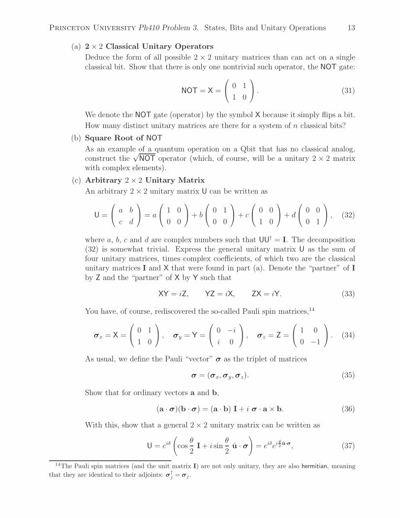
(a) 2 × 2 Classical Unitary Operators
Deduce the form of all possible 2 × 2 unitary matrices than can act on a singleclassical bit. Show that there is only one nontrivial such operator, the NOT gate:
NOT = X =
⎛⎝ 0 1
1 0
⎞⎠ . (31)
We denote the NOT gate (operator) by the symbol X because it simply flips a bit.
How many distinct unitary matrices are there for a system of n classical bits?
(b) Square Root of NOT
As an example of a quantum operation on a Qbit that has no classical analog,construct the
√NOT operator (which, of course, will be a unitary 2 × 2 matrix
with complex elements).
(c) Arbitrary 2 × 2 Unitary Matrix
An arbitrary 2 × 2 unitary matrix U can be written as
U =
⎛⎝ a b
c d
⎞⎠ = a
⎛⎝ 1 0
0 0
⎞⎠+ b
⎛⎝ 0 1
0 0
⎞⎠ + c
⎛⎝ 0 0
1 0
⎞⎠ + d
⎛⎝ 0 0
0 1
⎞⎠ , (32)
where a, b, c and d are complex numbers such that UU† = I. The decomposition(32) is somewhat trivial. Express the general unitary matrix U as the sum offour unitary matrices, times complex coefficients, of which two are the classicalunitary matrices I and X that were found in part (a). Denote the “partner” of Iby Z and the “partner” of X by Y such that
XY = iZ, YZ = iX, ZX = iY. (33)
You have, of course, rediscovered the so-called Pauli spin matrices,14
σx = X =
⎛⎝ 0 1
1 0
⎞⎠ , σy = Y =
⎛⎝ 0 −ii 0
⎞⎠ , σz = Z =
⎛⎝ 1 0
0 −1
⎞⎠ . (34)
As usual, we define the Pauli “vector” σ as the triplet of matrices
σ = (σx,σy,σz). (35)
Show that for ordinary vectors a and b,
(a · σ)(b · σ) = (a · b) I + i σ · a × b. (36)
With this, show that a general 2 × 2 unitary matrix can be written as
U = eiδ(
cosθ
2I + i sin
θ
2u · σ
)= eiδei
θ2u·σ, (37)
14The Pauli spin matrices (and the unit matrix I) are not only unitary, they are also hermitian, meaningthat they are identical to their adjoints: σ†
j = σj.

Princeton University Ph410 Problem 3. States, Bits and Unitary Operations 14
where δ and θ are real numbers and u is a real unit vector.15
What is the determinant of the matrix representation of U? The subset of 2 × 2unitary matrices with unit determinant is called the special unitary group SU(2).What is the version of eq. (37) that describes 2 × 2 special unitary operators?
Are the√
NOT operators found in part (b) special unitary operators?
You may wish to convince yourself of a factoid related to eq. (37), namely that ifA is a square matrix of any order such that A2 = I, then eiθA = cos θ I + i sin θ A,provided that θ is a real number. It follows that A can also be written in theexponential form
A = eiπ/2e−iπ2A = e−iπ/2ei
π2A. (38)
There are several unitary operators of interest, such as the Pauli matrices, thatare their own inverse. If we call such an operator V, then its exponential repre-sentation of V can be written in multiple ways,
V = eiδeiθ2v·σ = V−1 = e−iδe−i
θ2v·σ. (39)
(d) Why isn’t the operator Z of eq. (34) a valid 2 × 2 classical unitary operator?
(e) 2-Bit Classical Unitary Operations
How many 2-bit classical unitary operators are there?
While these operators can be expressed as 4 × 4 matrices, it is also instructive tocatalog them using 2× 2 matrices. For this, we regard a pair of Cbits x and y as
elements of a 2-dimensional vector,
⎛⎝ x
y
⎞⎠ .
Show that the number of 2-bit classical unitary operators is the same as thenumber of operators described by the transformations⎛
⎝ x
y
⎞⎠ →
⎛⎝ x′
y′
⎞⎠ = M
⎛⎝ x
y
⎞⎠⊕
⎛⎝ a
b
⎞⎠ , (40)
where M is an invertible 2 × 2 matrix (but not necessarily unitary), and a and bare constant Cbits. The symbol ⊕ means addition modulo 2, and the additionsresulting from the matrix multiplication are also modulo 2.
Since the matrices M are invertible, eq. (40) describes reversible transformations.Explain how/why these transformations are also unitary (and hence are represen-tations of all of the 2-bit classical unitary operators).
An important conclusion that can be drawn from the identification of 2-bit clas-sical unitary operators with the form (40) is that they are all linear functions ofthe input bits x and y.
It turns out that nonlinear, classical, unitary bit operators require 3 or moreQbits. Hence, the classical AND and OR operations will require 3 Qbits for aquantum implementation. See prob. 9.
15Note that if make the replacements θ → −θ and u → −u we obtain another valid representation of U,since the physical operation of a rotation by angle θ about an axis u is identical to a rotation by −θ aboutthe axis −u.
Princeton University Ph410 Problem 4. Rotation Matrices 15
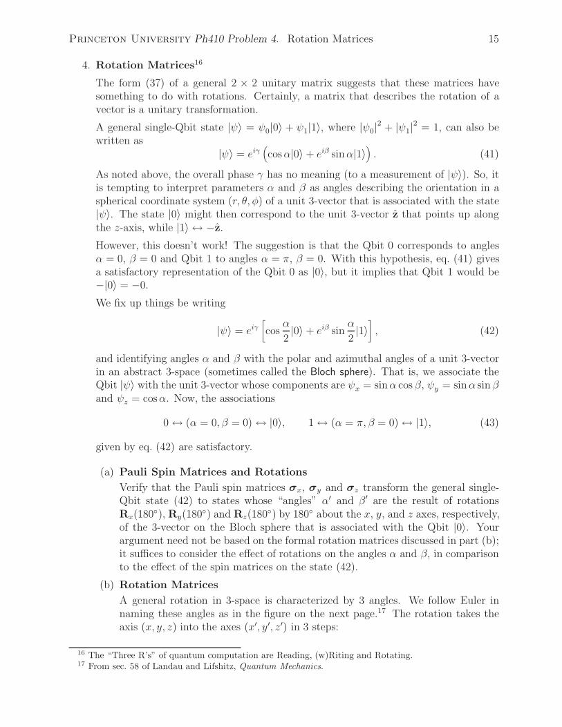
4. Rotation Matrices16
The form (37) of a general 2 × 2 unitary matrix suggests that these matrices havesomething to do with rotations. Certainly, a matrix that describes the rotation of avector is a unitary transformation.
A general single-Qbit state |ψ〉 = ψ0|0〉 + ψ1|1〉, where |ψ0|2 + |ψ1|2 = 1, can also bewritten as
|ψ〉 = eiγ(cosα|0〉 + eiβ sinα|1〉
). (41)
As noted above, the overall phase γ has no meaning (to a measurement of |ψ〉). So, itis tempting to interpret parameters α and β as angles describing the orientation in aspherical coordinate system (r, θ, φ) of a unit 3-vector that is associated with the state|ψ〉. The state |0〉 might then correspond to the unit 3-vector z that points up alongthe z-axis, while |1〉 ↔ −z.
However, this doesn’t work! The suggestion is that the Qbit 0 corresponds to anglesα = 0, β = 0 and Qbit 1 to angles α = π, β = 0. With this hypothesis, eq. (41) givesa satisfactory representation of the Qbit 0 as |0〉, but it implies that Qbit 1 would be−|0〉 = −0.
We fix up things be writing
|ψ〉 = eiγ[cos
α
2|0〉 + eiβ sin
α
2|1〉], (42)
and identifying angles α and β with the polar and azimuthal angles of a unit 3-vectorin an abstract 3-space (sometimes called the Bloch sphere). That is, we associate theQbit |ψ〉 with the unit 3-vector whose components are ψx = sinα cos β, ψy = sinα sin βand ψz = cosα. Now, the associations
0 ↔ (α = 0, β = 0) ↔ |0〉, 1 ↔ (α = π, β = 0) ↔ |1〉, (43)
given by eq. (42) are satisfactory.
(a) Pauli Spin Matrices and Rotations
Verify that the Pauli spin matrices σx, σy and σz transform the general single-Qbit state (42) to states whose “angles” α′ and β′ are the result of rotationsRx(180
◦), Ry(180◦) and Rz(180
◦) by 180◦ about the x, y, and z axes, respectively,of the 3-vector on the Bloch sphere that is associated with the Qbit |0〉. Yourargument need not be based on the formal rotation matrices discussed in part (b);it suffices to consider the effect of rotations on the angles α and β, in comparisonto the effect of the spin matrices on the state (42).
(b) Rotation Matrices
A general rotation in 3-space is characterized by 3 angles. We follow Euler innaming these angles as in the figure on the next page.17 The rotation takes theaxis (x, y, z) into the axes (x′, y′, z′) in 3 steps:
16 The “Three R’s” of quantum computation are Reading, (w)Riting and Rotating.17 From sec. 58 of Landau and Lifshitz, Quantum Mechanics.

Princeton University Ph410 Problem 4. Rotation Matrices 16
i. A rotation by angle α about the z-axis, which brings the y-axis to the y1 axis.
ii. A rotation by angle β about the y1-axis, which brings the z-axis to the z′-axis.
iii. A rotation by angle γ about the z′-axis, which brings the y1-axis to the y′-axis(and the x-axis to the x′-axis).
The 2 × 2 unitary matrix that corresponds to this rotation is
R(α, β, γ) =
⎛⎝ cos β
2ei(α+γ)/2 sin β
2ei(−α+γ)/2
− sin β2ei(α−γ)/2 cos β
2e−i(α+γ)/2
⎞⎠
=
⎛⎝ eiγ/2 0
0 e−iγ/2
⎞⎠⎛⎝ cos β
2sin β
2
− sin β2
cos β2
⎞⎠⎛⎝ eiα/2 0
0 e−iα/2
⎞⎠
= Rz′ (γ)Ry1(β)Rz(α), (44)
where the decomposition into the product of 3 rotation matrices18 follows fromthe particular rules
Rx(φ) =
⎛⎝ cos φ
2i sin φ
2
i sin φ2
cos φ2
⎞⎠ , (45)
Ry(φ) =
⎛⎝ cos φ
2sin φ
2
− sin φ2
cos φ2
⎞⎠ , (46)
Rz(φ) =
⎛⎝ eiφ/2 0
0 e−iφ/2
⎞⎠ . (47)
Convince yourself that the combined rotation (44) could also be achieved if firsta rotation is made by angle γ about the z axis, then a rotation is made by angleβ about the original y axis, and finally a rotation is made by angle α about theoriginal z axis.
18 The order of operations is that the rightmost rotation in eq. (44) is to be performed first.

Princeton University Ph410 Problem 4. Rotation Matrices 17
There is unfortunately little consistency among various authors as to the conven-tions used to describe rotations. I will now adopt the notation of Barenco et al.,19
who appear to write eq. (44) simply as
R(α, β, γ) = Rz(γ)Ry(β)Rz(α). (48)
Occasionally (for example in part (c)) we will need to remember that in eq. (48) theaxes of the second and third rotations are the results of the previous rotation(s).
Also, Nielsen and Chuang consider rotations to be by the negative of the anglesthat I do. Thus, the operator that I call Rx(φ) is called Rx(−φ) by them.
Note that according to eqs. (45)-(47),
σx = −iRx(180◦), σy = −iRy(180◦), σz = −iRz(180◦), (49)
and also
σx = iRx(−180◦), σy = iRy(−180◦), σz = iRz(−180◦), (50)
so that the Pauli spin matrices are equivalent to the formal matrices for 180◦
rotations only up to a phase factor i.
Show that a more systematic relation between the Pauli spin matrices and therotation matrices is that eqs. (45)-(47) can be written as
Ru(φ) = eiφ2u·σ, (51)
which describes a rotation of the coordinate axes in Bloch space by angle φ aboutthe u axis (in a right-handed convention).
Rather than rotating the coordinate axes, we may wish to rotate vectorsin Bloch space by an angle φ about a given axis u, while leaving thecoordinate axes fixed. The operator
Ru(−φ) = e−iφ2u·σ (52)
performs this type of rotation.
Equations (50) and (51) can be combined to write20
σj = ie−iπ2σj = ei
π2 e−i
π2σj , (53)
which permits us to define an arbitrary power of a Pauli matrix as21
σαj = (eiπ2 e−i
π2σj )α = ei
πα2 e−i
πα2
σj . (54)
Show that the phase gate with phase angle φ = πα can be written as⎛⎝ 1 0
0 eiπα
⎞⎠ = σαz = Zα. (55)
19 http://physics.princeton.edu/~mcdonald/examples/QM/barenco_pra_52_3457_95.pdf20This also follows from eq. (38).21Since the Pauli matrices are their own inverses, it is tempting to write σα
j = e−i πα2 ei πα
2 σj = σ−αj .
However, this relation is not true in general, because fractional powers of the Pauli matrices correspond torotations by angles that are a fraction of π, so the direction of the rotation matters.

Princeton University Ph410 Problem 4. Rotation Matrices 18
(c) More Square Roots of NOT
Use the facts about rotation matrices presented in part (b) to construct additionalrepresentations of the NOT and
√NOT operators that act on Qbit
|ψ〉 = ψ0|0〉 + ψ1|1〉, supposing that the overall phase of |ψ〉 is irrelevant. Recallthat the basic intent of the NOT operator is to flip the bits 0 and 1.
(d) Rotation Matrices and the General Form (37)
From eq. (44) we see that the determinant of R(α, β, γ) is unity, so that there isa one-to-one correspondence between rotation matrices and 2× 2 special unitaryoperators. Recalling the general form (37), we also infer that a general 2 × 2unitary operator U can be written as
U = eiδR(α, β, γ) = eiδRz(γ)Ry(β)Rz(α). (56)
What is the relation between parameters α, β and γ of eq. (56) and the parametersθ and u of eq. (37)?
(e) Double NOT
Among the many identities involving rotation matrices, demonstrate that
σxUσx = XeiδR(α, β, γ)X = eiδR(−α,−β,−γ), (57)
which will be used later in the course.
(f) Basis Change
The result of a rotation R in 3-space can be thought of as a change of basis fromthe orthonormal triad (x, y, z) to a new orthonormal triad (x′, y′, z′) = R(x, y, z).
Similarly, a 2 × 2 unitary matrix
U =
⎛⎝ a b
c d
⎞⎠ (58)
can be thought of as causing a change from the basis of orthonormal states(|0〉, |1〉) to a new orthonormal basis
|ψ〉 = U|0〉 = a|0〉 + c|1〉, |φ〉 = U|1〉 = b|0〉 + d|1〉. (59)
Verify that the states |ψ〉 and |φ〉 are indeed orthonormal.
(g) Hadamard Transformation
It will be of interest on occasion to switch from the basis [|0〉, |1〉] (or simply the[0, 1] basis) to the basis [(|0〉+|1〉)/√2, (|0〉−|1〉)/√2] (which we will often call the[|+〉, |−〉] or the [+,−] basis). The unitary matrix that performs this operation iscalled the Hadamard transformation (or gate):
H =1√2
⎛⎝ 1 1
1 −1
⎞⎠ =
X + Z√2
=σx + σz√
2. (60)
We see that H is self-adjoint, so that H2 = I; a second application of the Hadamardtransformation brings us back to the original basis.

Princeton University Ph410 Problem 4. Rotation Matrices 19
Express the Hadamard transformation in the general forms (37) and (51).
It is sometimes useful to write the effect of the Hadamard transformation on abasis state |j〉, where j = 0 or 1, as
H|j〉 =|0〉 + (−1)j |1〉√
2=
|0〉 + eiπj|1〉√2
. (61)
(h) Show that the Pauli spin matrices and the Hadamard transformation are relatedby identities such as
σαx = HσαzH, (62)
σαy = σ1/2z σαxσ
−1/2z , (63)
Hα = σ1/4y σαzσ
−1/4y , (64)
which implies that all of σαx , σαy , σ
αz and Hα can be constructed from only H and
σαz .
(i) For use later in the course, it will be useful to know a relation between the
rotation Ru(θ) = eiθ2u·σ by an arbitrary angle θ about an axis u and a rotation
Rv(θ) = eiθ2v·σ by the same angle about an axis v that is perpendicular to u.
Show thatH−1/2 ei
θ2u·σ H1/2 (65)
corresponds to a rotation by angle θ about an axis v (whose components you areto find in terms of those of u), and deduce a condition on u such that u · v = 0.
(j) Basis States for the Hadamard Transformation
From the definition (60) of the Hadamard transformation H with respect to the[|0〉, |1〉] basis, we have that
H|0〉 = |+〉 =|0〉 + |1〉√
2, and H|1〉 = |−〉 =
|0〉 − |1〉√2
. (66)
From the fact that H2 = I we then find
H|+〉 = |0〉 =|+〉 + |−〉√
2, and H|−〉 = |1〉 =
|+〉 − |−〉√2
. (67)
Show that the set of all orthonormal bases [|ψ〉, |φ〉] for which
H|ψ〉 =|ψ〉 + |φ〉√
2, and H|φ〉 =
|ψ〉 − |φ〉√2
. (68)
describe a cone on the unit Bloch sphere whose axis is at 45◦ to the x and z axesin the x-z plane.
If we define the basis state |ψ〉 according to eq. (42),
|ψ〉 = eiγ[cos
α
2|0〉 + eiβ sin
α
2|1〉], (42)

Princeton University Ph410 Problem 4. Rotation Matrices 20
where (α, β) are the polar and azimuthal angles of the vector |ψ〉 on the Blochsphere, then the orthogonal vector |φ〉 has polar angle π−α and azimuthal angleβ + π. Thus, we can write
|φ〉 = eiδ[sin
α
2|0〉 − eiβ cos
α
2|1〉], (69)
where only the difference between phases γ and δ has physical significance. Hence,you can, for example, set phase γ to zero in your solution without loss of generality,but you cannot necessarily set both γ and δ to zero.

Princeton University Ph410 Problem 5. Measurements 21
5. Measurements
In a computational context, the most common kind of measurement we will make ona Qbit |ψ〉 = ψ0|0〉 + ψ1|1〉 is a determination of whether that Qbit is a |0〉 or a |1〉.For example, if we wish to find out whether |ψ〉 is |0〉 we could apply the operator
P0 = |0〉〈0| =
⎛⎝ 1 0
0 0
⎞⎠ (70)
to it, with the resultP0|ψ〉 = ψ0|0〉. (71)
What can this mean in practice?
That the quantum state |ψ〉 can be subject to an operator P0 implies that there is moreto the universe than state |ψ〉 itself. The universe must contain additional entities thatprovide the physical implementation of the operator P0, as well as some mechanism forrecording the result of that operation. We do not wish to embark now on the lengthydetour to explore the full meaning of the previous sentence. We note that Bohr andHeisenberg considered that the system which makes the measurement must have a“classical” component, but they remained somewhat vague as to the nature of thedivide between the classical and quantum parts of the system. I too will be somewhatvague now, but we will return to this topic in prob. 20.

Princeton University Ph410 Problem 5. Measurements 22
We presume that the operator P0 can be implemented in such a way that its effect onthe entire system is either1. The state |ψ〉 is projected into state |0〉 and the larger system is left with a recordthat |0〉 was found to be (or projected into, if you prefer) the state |0〉,or,2. The larger system is left with no record that state |0〉 was found to be |0〉, and thestate |ψ〉 is left as |ψ′〉 = (|ψ〉−ψ0|0〉)/〈ψ ′|ψ′〉, which is simply |ψ′〉 = |1〉 in the presentexample.If we had many copies of |ψ〉 on which to make measurements, the probability thatstate |ψ〉 was found to be |0〉 would be |ψ0|2 = 〈ψ|P†
0P0|ψ〉.
Similarly, we associate operator
P1 = |1〉〈1| =
⎛⎝ 0 0
0 1
⎞⎠ (72)
with a measurement of to what extent state |ψ〉 is state |1〉.Neither the projection operator P0 nor P1 represents a measurement by itself. Rather,a measurement should provide us with information as to what extent state |ψ〉 is ineither of its basis states |0〉 and |1〉. We express this more formally by defining ameasurement M to determine the “value” of Qbit |ψ〉 by associating the outcome withthe (“classical”) quantity 0 if |ψ〉 is found to be |0〉 and with 1 if |ψ〉 is found to be|1〉. We will write the measurement M as
M = 0 · P0 + 1 · P1, (73)
where we place the symbol · between the (“classical”) value vj and its correspondingprojection operator |j〉〈j| to remind us that the effect of the operation vj · |j〉〈j| is toproject state |ψ〉 into state |j〉 while returning value vj for the measurement.
Both operators P0 and P1 are hermitian, since P†0 = P0 and P†
0 = P1. This illus-trates a general quantum rule: measurable quantities (observables) are associated withhermitian operators.
We now generalize to states other than a single Qbit, but where a quantum state |ψ〉can be represented via a set of orthonormal basis states {|φj〉},
|ψ〉 =∑j
ψj|j〉, where 〈j|k〉 = δjk. (74)
We will only consider so-called projective measurements for which each basis state |j〉is an eigenvector of a hermitian operator Mj with eigenvalue mj:
Mj |j〉 = mj · |j〉. (75)
The hermitian operatorM =
∑j
Mj (76)

Princeton University Ph410 Problem 5. Measurements 23
is associated with a measurement to determine the value of the variable m whosepossible values are the set {mj}.22 Comparing with the discussion for the projectionoperators (70) and (72), we see that the jth measurement operator, Mj, is simplyrelated to the projection operator Pj, defined by
Pj = |j〉〈j|, for which P†j = P2
j = Pj. (77)
That is,Mj = mj · Pj = mj · |j〉〈j|. (78)
Hence, in the [|j〉] basis, the operator
M =∑j
Mj =∑j
mj · Pj =∑j
mj · |j〉〈j| (79)
is diagonal, when expressed as a matrix.
The hermitian measurement operator (79) projects the state |ψ〉 onto one of the basisstates |j〉, and returns the value mj in that case. The probability that the result of theprojection is state |j〉 is
Pj = 〈ψ|P†jPj |ψ〉 = 〈ψ|Pj|ψ〉 = 〈ψ|j〉〈j|ψ〉 = |〈j|ψ〉|2 (80)
The total probability of finding some result of the measurement is, of course, unity:
1 =∑j
Pj =∑j
〈ψ|P†jPj|ψ〉 =
∑j
|〈j|ψ〉|2 (81)
A measurement M|ψ〉 can only return a single value, say mj, in which case the finalstate of |ψ〉 (the value mj is recorded elsewhere in the measuring apparatus) is
Pj|ψ〉√〈ψ|P†
jPj|ψ〉=
Pj |ψ〉|〈j|ψ〉| , (82)
rather than Pj |ψ〉. A measurement is a physical process, and so must also be associatedwith a transformation that preserves the normalization of a state, as does the form(82).23
The probable value (or expectation value) of variable m for state |ψ〉 is thus
〈m〉 =∑j
mjPj =∑j
mj〈ψ|Pj|ψ〉 = 〈ψ|∑j
mj · Pj|ψ〉 = 〈ψ|M|ψ〉. (83)
This important relation is still true when the state |ψ〉 is expressed in some other basisthan the [|j〉] basis, in which the hermitian matrix M is no longer diagonal.
22If the index j in eq. (76) does not run over a complete set of basis states the operator M represents onlya partial measurement. A common example of this is a filter, such as a polarizing filter than can absorb(measure) photons of one polarization while transmitting photons of the orthogonal polarization.
23An aspect of the “measurement problem” of quantum mechanics is that the transformation of state|ψ〉 to state (82) is not reversible, and so is not expressible as a unitary transformation (even though totalprobability is preserved).
Princeton University Ph410 Problem 5. Measurements 24
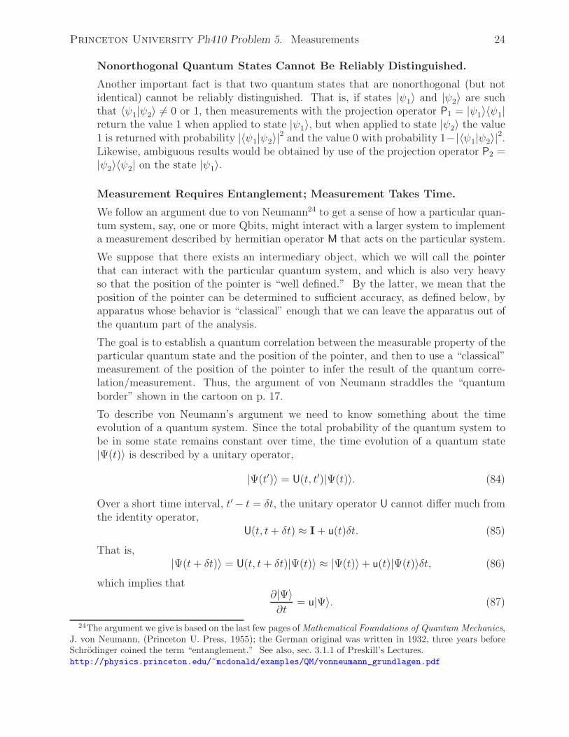
Nonorthogonal Quantum States Cannot Be Reliably Distinguished.
Another important fact is that two quantum states that are nonorthogonal (but notidentical) cannot be reliably distinguished. That is, if states |ψ1〉 and |ψ2〉 are suchthat 〈ψ1|ψ2〉 = 0 or 1, then measurements with the projection operator P1 = |ψ1〉〈ψ1|return the value 1 when applied to state |ψ1〉, but when applied to state |ψ2〉 the value1 is returned with probability |〈ψ1|ψ2〉|2 and the value 0 with probability 1−|〈ψ1|ψ2〉|2.Likewise, ambiguous results would be obtained by use of the projection operator P2 =|ψ2〉〈ψ2| on the state |ψ1〉.
Measurement Requires Entanglement; Measurement Takes Time.
We follow an argument due to von Neumann24 to get a sense of how a particular quan-tum system, say, one or more Qbits, might interact with a larger system to implementa measurement described by hermitian operator M that acts on the particular system.
We suppose that there exists an intermediary object, which we will call the pointerthat can interact with the particular quantum system, and which is also very heavyso that the position of the pointer is “well defined.” By the latter, we mean that theposition of the pointer can be determined to sufficient accuracy, as defined below, byapparatus whose behavior is “classical” enough that we can leave the apparatus out ofthe quantum part of the analysis.
The goal is to establish a quantum correlation between the measurable property of theparticular quantum state and the position of the pointer, and then to use a “classical”measurement of the position of the pointer to infer the result of the quantum corre-lation/measurement. Thus, the argument of von Neumann straddles the “quantumborder” shown in the cartoon on p. 17.
To describe von Neumann’s argument we need to know something about the timeevolution of a quantum system. Since the total probability of the quantum system tobe in some state remains constant over time, the time evolution of a quantum state|Ψ(t)〉 is described by a unitary operator,
|Ψ(t′)〉 = U(t, t′)|Ψ(t)〉. (84)
Over a short time interval, t′ − t = δt, the unitary operator U cannot differ much fromthe identity operator,
U(t, t+ δt) ≈ I + u(t)δt. (85)
That is,|Ψ(t+ δt)〉 = U(t, t+ δt)|Ψ(t)〉 ≈ |Ψ(t)〉+ u(t)|Ψ(t)〉δt, (86)
which implies that∂|Ψ〉∂t
= u|Ψ〉. (87)
24The argument we give is based on the last few pages of Mathematical Foundations of Quantum Mechanics,J. von Neumann, (Princeton U. Press, 1955); the German original was written in 1932, three years beforeSchrodinger coined the term “entanglement.” See also, sec. 3.1.1 of Preskill’s Lectures.http://physics.princeton.edu/~mcdonald/examples/QM/vonneumann_grundlagen.pdf

Princeton University Ph410 Problem 5. Measurements 25
The famous insight of Schrodinger is that if we write
u = − i
hH = −ih, (88)
then the operator H = hh is not the Hadamard transformation but is related tothe Hamiltonian of the system in a well-defined manner. Thus, eq. (87) becomesSchrodinger’s equation
id|Ψ〉dt
= h|Ψ〉. (89)
Since the operator U ≈ I − ihδt is unitary, U−1 = U† ≈ I + ih†δt. Then,
1 = U−1U ≈ (I + ih†δt)(I − ihδt) ≈ I + i(h† − h)δt, (90)
so that we must have h† = h, i.e., the Hamiltonian operator is hermitian.
Returning to the case of a particular quantum system plus the pointer, we take theHamiltonian of the combined system to be of the form
h = h0 +p2
2m+ λMp ≈ λMp, (91)
where h0 is the Hamiltonian of the particular system when in isolation, p = −i∂/∂x isthe momentum operator of the pointer (which can move only in the x direction), m isthe (large) mass of the pointer, λ is a coupling constant, and M is the measurementoperator that applies to the particular quantum system. The approximate form of theHamiltonian follows on noting that mass m is large, and that during the measurementthe effect of the interaction term λMp is much larger than that of isolated Hamiltonianh0 (otherwise the measurement could not produce a crisp result25).
The state of the particular system to be measured is
|ψ〉 =∑j
ψj|j〉, (92)
and the initial state of the pointer is |φ(x)〉, which is a Gaussian wave packet centeredon, say, x = 0, normalized such that
∫ |φ(x)|2 dx = 1. Since the pointer particle isheavy, its wave packet |φ(x)〉 is narrow (but not so narrow that the wave packet spreadssignificantly during the measurement). The initial state of the combined system is thedirect product
|Ψ(0)〉 = |ψ〉 ⊗ |φ(x)〉 =∑j
ψj |j〉 ⊗ |φ(x)〉. (93)
The basis [|j〉] for the particular system has been chosen so that the each basis state |j〉has a well-defined value mj of the measurement. That is, the measurement operatorhas the projective form
M =∑j
mj · |j〉〈j|. (94)
25See, for example, http://physics.princeton.edu/~mcdonald/examples/QM/peres_prd_32_1968_85.pdf

Princeton University Ph410 Problem 5. Measurements 26
The Hamiltonian h ≈ λMp is time independent, so Schrodinger’s equation (89) has theformal solution
|Ψ(t)〉 = e−iht|Ψ(0)〉. (95)
Now
e−iht =∞∑n=0
(−iht)nn!
=∞∑n=0
1
n!
⎡⎣−iλ∑
j
mj · |j〉〈j|(−i ∂∂x
)t
⎤⎦n
=∑j
|j〉〈j|∞∑n=0
1
n!
(−λmjt
∂
∂x
)n, (96)
recalling that 〈j|k〉 = δjk, so that the lengthy products of bras and kets all collapseback down to the projections |j〉〈j|. Inserting eqs. (93) and (96) into (95), we obtain
|Ψ(t)〉 =∑j
|j〉〈j|∑k
ψk|k〉 ⊗∞∑n=0
1
n!
(−λmjt
∂
∂x
)n|φ(x)〉
=∑j
ψj |j〉 ⊗ |φ(x− λmjt)〉, (97)
noting that the Taylor expansion of φ(x− x0) is
φ(x− x0) =∞∑n=0
1
n!
(−x0
∂
∂x
)nφ(x). (98)
The initial direct product state (93) has evolved into the entangled state (97) duringthe course of the measurement.
The supposition is that the position of the pointer at time t can be determined wellenough to distinguish the j locations λmjt from one another. If the pointer is found at(or near) position λmjt, the particular system |ψ〉 must be in state |j〉 and the value ofthe measurement is mj. The probability that this is the outcome of the measurement
is, of course,∣∣∣ψj∣∣∣2 since
∫ |φ(x− λmjt)| dx = 1.
This argument does a nice job of explaining how to entangle the state |ψ〉 =∑ψj |j〉
with a pointer such that different positions of the pointer are correlated with differentbasis states |j〉. However, it does not explain how the observation of the position of thepointer to be, say, λmjt “collapses the wave function” of |ψ〉 to the basis state |j〉.26
Von Neumann’s argument indicates that underlying every measurement process is theentanglement that bothered Einstein, Podolsky and Rosen (and Schrodinger, etc.) somuch. This deserves further discussion, some of which will be given in prob. 20.
26The transformation from |Ψ(0)〉 to |Ψ(t)〉 is unitary/reversible as eq. (97) is valid for both increasing ordecreasing t. The irreversible step in the measurement process is the “classical” reading of the position ofthe pointer at time tmeas, which selects a value of x ≈ λmjtmeas and leaves the system in the state
|Ψ(t > tmeas)〉 =|j〉 ⊗ |φ(x− λmjtmeas)〉√
N, (99)
where N is the number of possible positions of the pointer.

Princeton University Ph410 Problem 5. Measurements 27
Problems.
(a) Consider the hermitian operator (that acts on a single Qbit)
v · σ = vxX + vyY + vzZ, (100)
where v is a real unit vector, i.e., v2x + v2
y + v2z = 1. What are the eigenvalues and
eigenvectors of the operator v · σ? Hint: recall eq. (42).
What are the projection operators onto those eigenvectors?
What is the probability of obtaining the result +1 for a measurement of v · σon the state |0〉? What is the state after the measurement if the result +1 isobtained?
(b) Suppose the state |ψ〉 consists of two Qbits in the entangled form
|ψ〉 = ψ00|0〉|0〉 + ψ01|0〉|1〉 + ψ10|1〉|0〉 + ψ11|1〉|1〉. (101)
What is the state |ψ′〉 after a measurement to determine the value of the secondbit? What is the probability that the second bit is found to have value 1 in thismeasurement?
Suppose we wish to measure the values of both the first and second bits. Whatis the appropriate measurement operator? How does this operator determine theprobabilities that the two bits are |0〉|0〉, |0〉|1〉, |1〉|0〉 or |1〉|1〉?
(c) Stern-Gerlach. The argument of eqs. (91)-(98) can be generalized to the caseof a pointer whose value is described by a coordinate q by use of a Hamiltonianthat couples the system to be measured to the canonical momentum p that isconjugate to q. That is, consider h ≈ λMp where p = −i∂/∂q.Use this fact to describe how a Stern-Gerlach apparatus “measures” the z-componentof the spin of a neutral spin-1/2 particle that is moving in the x direction throughmagnetic field B ≈ B(z) z. Recall that such an apparatus gives a “kick” to theparticle in the z-direction whose sign depends on whether the spin is “up” or“down.”
It suffices to display an appropriate Hamiltonian for the system.
(d) Quantum Nondemolition Measurement.27 The prescription (97) for theentanglement of a state |ψ〉 with the pointer state |φ〉 permits, in principle, thestate |ψ〉 to be measured without being destroyed. Ideally, quantum measurementis a nondemolition process. However, in examples such as photons, the state tobe measured is typically destroyed in the process. In such cases a nondemolitionmeasurement could be made if the state |ψ〉 =
∑j aj|j〉 were first entangled with
another state |φ〉 such that the result is |ψ〉|φ〉 =∑j aj|j〉|j〉. Then, a destructive
measurement of state |φ〉 leaves state |ψ〉 in a known, and still existing, basisstate.
Deduce the form of a symmetric, unitary 4 × 4 matrix U that operates on Qbits|ψ〉 = a0|0〉 + a1|1〉 and |φ〉 = |0〉 according to U|ψ〉|φ〉 = a0|0〉|0〉 + a1|1〉|1〉.That we could not simply make a copy of the (unknown) quantum state |ψ〉 beforemeasuring it is the topic of Prob. 6.
27We use the term quantum nondemolition measurement in a slightly different way than in which it wasintroduced historically. See, http://physics.princeton.edu/~mcdonald/examples/QM/caves_rmp_52_341_80.pdf

Princeton University Ph410 Prob. 6. Quantum Cloning, Quantum Teleportation 28
6. Quantum Cloning, Quantum Teleportation
We have previously remarked that the amplitudes of the various eigenstates of a generalquantum state |ψ〉 =
∑ψj|j〉 cannot be determined by a single measurement, or even
a finite set of measurements should many copies of the state be available. It mighttherefore be considered “obvious” that an exact copy of this quantum state cannot bemade, unless the amplitudes ψj are known a priori. However, it appears that this factwas never explicitly noted prior to 1982.28
We demonstrate the no-cloning theorem by contradiction. We first suppose that aunitary cloning operator C exists that acts on the zero state |0〉 and an arbitrary Qbit|ψ〉 such that state |ψ〉 is unchanged while |0〉 turns into |ψ〉. Thus, C is defined by
C|ψ〉|0〉 = |ψ〉|ψ〉. (102)
This should work for another state |φ〉 as well:
C|φ〉|0〉 = |φ〉|φ〉. (103)
Since C is unitary, it preserves the inner product,
〈φ|ψ〉 = 〈0|〈φ|ψ〉|0〉 = 〈0|〈φ|C†C|ψ〉|0〉 = 〈φ|〈φ|ψ〉|ψ〉 = (〈φ|ψ〉)2. (104)
However, eq. (104) can be true only if 〈φ|ψ〉 = 0 or 1. If |ψ〉 and |φ〉 are not orthogonalthe operator C cannot have successfully copied them both. Hence, the general cloningoperator C does not exist.
We see that there is no problem copying an unknown single-bit state if it can only be|0〉 or |1〉. This is what classical copying does, which operation could, therefore, beimplemented by a quantum device.
However, we see that the result of a quantum computation cannot be in the form ofa general quantum state, if we are to copy it exactly for further use. The result mustbe expressed as one of a set of orthogonal states, in which case we could in principlemeasure/copy the result without altering it.29
Hence, some of the richness of information content of a general quantum state is in-evitably lost at the end of a practical quantum computation. Nonetheless, quantumcomputation can still have many advantages over classical computation.
Quantum Money. S. Wiesner anticipated the no-cloning theorem to some extentin 1970,30 when he proposed that “quantum money” could not be counterfeited if itsserial number consisted of a string of bits each of whose base is randomly chosen atthe “mint” to be either [0,1] or [+,−]. A counterfeiter who measured the bits beforeduplicating the “money” would, on average, be able to duplicate correctly only 50% ofthe bits. A “bank” must know the “mint’s” choice of bases to detect the counterfeit.
28 http://physics.princeton.edu/~mcdonald/examples/QM/wootters_nature_299_802_82.pdfhttp://physics.princeton.edu/~mcdonald/examples/QM/dieks_pl_a92_271_82.pdf
29Compare with the lesson of Maxwell’s Demon (prob. 2): to “know” a state means that we can copy it.30 http://physics.princeton.edu/~mcdonald/examples/QM/wiesner_70.pdf

Princeton University Ph410 Prob. 6. Quantum Cloning, Quantum Teleportation 29
(a) Copying of a classical bit |x〉 onto a second Cbit |y〉 whose initial state is |0〉can be accomplished by a unitary transformation Cxy that leaves bit |y〉 alone if|x〉 = 0 but flips bit |y〉 if |x〉 = |1〉. Express the two-bit operator Cxy as a 4 × 4matrix that acts on the basis
|x〉|y〉 =
⎛⎝ x0
x1
⎞⎠⊗
⎛⎝ y0
y1
⎞⎠ =
⎛⎜⎜⎜⎜⎜⎜⎝
x0y0
x0y1
x1y0
x1y1
⎞⎟⎟⎟⎟⎟⎟⎠, such that |0〉|1〉 =
⎛⎜⎜⎜⎜⎜⎜⎝
0
1
0
0
⎞⎟⎟⎟⎟⎟⎟⎠, etc.
(105)
The operator Cxy is called the Controlled-NOT because it flips the second bit, |y〉,only on the condition that the first bit, |x〉, is 1.31
We take this occasion to introduce a graphical representation of bit operationsthat will be used extensively throughout the course. The history of a bit is shownon a horizontal line, and bit operations are indicated in boxes. Thus, the figureon the left below indicates that the NOT operation, X, is applied to a Qbit |a〉.The Controlled-NOT operation Cab, shown schematically in the righthand figure,involves 2 Qbits, |a〉 and |b〉. The first bit is called the control bit, whose effect isindicated by a solid circle with a vertical line connected to the box representingthe NOT operation on the second bit (the target bit), meaning that target bit issubject to the NOT operation only if the control bit is in the |1〉 state.
I will use the convention that the flow of logic is from left to right in the bit-operation diagrams. Note, however, that some people use a right-to-left flow(without arrows to guide the eye), perhaps because in Dirac’s bra-ket notation theinput ket is on the right. Of course, since quantum bit operations are reversible,the flow of logic can be in either direction.
What is the state |y〉 obtained by applying the Controlled-NOT operation to |x〉|0〉when |x〉 is the general Qbit a|0〉+ b|1〉? For what states |x〉 is |y〉 an exact copy?
Despite the failure of the Controlled-NOT operator to copy successfully a generalQbit, it will become our favorite 2-bit operator.
Show that if we have two copies, |x〉 and |y〉, of a Cbit (perhaps obtained by useof the Controlled-NOT operation), then applying Cxy to the pair will delete thesecond bit, i.e., transform it to the bit |0〉. Show, however, that the Controlled-NOT operation cannot be used to delete the second of two copies (obtaining bypreparation rather than by copying!) of a general Qbit. This illustrates theno-deleting theorem.32
(b) Successful Cloning Would Imply Faster-Than-Light Communication
Show that exact cloning of an arbitrary quantum state could lead to a schemefor faster-than-light communication. In particular, consider an entangled state of
31In the language of classical computation, the Controlled-NOT operation is the XOR = exclusive ORoperation (logic gate).
32 http://physics.princeton.edu/~mcdonald/examples/QM/pati_nature_404_164_00.pdf

Princeton University Ph410 Prob. 6. Quantum Cloning, Quantum Teleportation 30
two Qbits:|ψ〉 =
|00〉 + |11〉√2
=|0〉A|0〉B + |1〉A|1〉B√
2, (106)
such that after creation of this state the physical realizations of the first andsecond bits become separated in space. A famous example of this is the S-wavedecay of an excited atom via two back-to-back photons.
Observer A (Alice) can chose to observe bit A in the basis [|0〉, |1〉], or in the basis[(|0〉 + |1〉)/√2, (|0〉 − |1〉)/√2] ≡ [|+〉, |−〉] (among the infinite set of bases for asingle Qbit), and the choice of which basis she uses can be delayed; i.e., Alice canwait to choose her observational basis until after the bits A and B have separatedin space.
The “message” that Alice wishes to send to observer B (Bob) is her choice of basisfor observation of bit A, and the result of her observation.
If the state (106) cannot be cloned, Bob can make only a single observation, andmust choose a single basis (either [|0〉, |1〉] or [|+〉, |−〉]) for this.
Describe the possible correlations between the results of measurements by Aliceon bit A with the results of measurements by Bob on bit B, given that both Aliceand Bob can choose to use either the [|0〉, |1〉] or the [|+〉, |−〉] bases. Can themeasurements made by Bob, in the absence of classical communication from Aliceas to the nature of her measurements, be interpreted by Bob as certain knowledgeby him as to which choice of basis was made by Alice? To answer this, it is helpfulto re-express state (106) in the [|+〉, |−〉] basis.
You may or may not find it helpful to construct and apply measurement operatorsto the appropriate representations of the entangled state of bits A and B.
Now suppose that Bob could clone his bit B in such a manner that the clonesretained the entangled structure of state (106). Describe a set of measurementson these clones that would permit Bob to know with certainty (i.e., with veryhigh probability) what choice of basis had been made by Alice. Since Alice andBob could, in principle, be separated by arbitrarily large distances at the timesthat they make their measurements, successful deduction by Bob as to Alice’schoice of basis would imply an “instantaneous” communication from Alice
The above scenario was presented in 1982 by Herbert,33 which appears to havebeen a strong motivation for the formulation of the no-cloning theorem.34
Note: You may not be able to reproduce Herbert’s logic that led to his claim thatfaster-than-light communication is possible, as he never wrote down the form of
33 http://physics.princeton.edu/~mcdonald/examples/QM/herbert_fp_12_1171_82.pdf34To me, the statement of the no-cloning theorem in 1982 marks the end of a somewhat nonproductive
era in which numerous people used variants on the Einstein-Podolsky-Rosen argument (footnote 8, p. 12) tolook for defects in quantum mechanics. A popular hope was that there might exist “hidden variables” thatmore completely characterized a quantum state than a description such as eq. (11). But if a more completecharacterization existed, we might expect that cloning of an arbitrary quantum state would be possible.Hence, to me, the no-cloning theorem is a simple yet strong indication (much simpler than the convolutedarguments related to Bell’s inequalities) that the search for hidden variables is misguided. After 1982 therehas been a much healthier emphasis on uses of entanglement to explore the greater richness of quantumcompared to classical phenomena.

Princeton University Ph410 Prob. 6. Quantum Cloning, Quantum Teleportation 31
his quantum state including clones of bit B. He desires that all the clones of bitB are entangled with a single bit A.35
Consider the option that Bob makes a “copy” of bit B via a Controlled-NOT gatewhose second input line, bit C, is initially |0〉. The resulting entangled state ofbits A, B and C is as good a copy of state (106) as possible. Show, however, thatmeasurements by Bob of bit B in the [0,1] basis and of bit C in the [+,−] basis,as proposed by Herbert, do not add Bob’s knowledge of bit A.36
(c) Bit Swapping
We cannot make an exact copy of an arbitrary quantum state, but we can swaptwo arbitrary states (that consist of the same number of Qbits).
Construct an operation Sab (a 4×4 unitary matrix) that swaps two Cbits a and b.Show how Sab can be implemented as a sequence of Controlled-NOT operations,noting that Cab and Cba are distinct.37 Draw a bit-flow diagram for this sequence.38
Verify that Sab swaps two arbitrary Qbits |a〉 = α|0〉+ β|1〉 and |b〉 = γ|0〉+ δ|1〉.(d) Quantum Teleportation
In 1993, Bennett et al.39 developed a scheme for transforming an arbitrary Qbitin a very intriguing fashion that they described as quantum teleportation (althoughthis provocative name perhaps overdramatizes the significance of this transforma-tion). We illustrate this with a variant due to Brassard et al.40
Consider the sequence of operations on 3 Qbits sketched in the figure below. Theinitial Qbit |a〉 is arbitrary, while the initial Qbits |b〉 and |c〉 are both |0〉.
Show that despite the entangling effects of the Hadamard transformations, thefinal state is a direct product, |a′b′c′〉 = |a′〉|b′〉|c′〉, where |a′〉 and |b′〉 are indepen-dent of |a〉, and |c′〉 = |a〉. Thus, this process transfers the (unknown) character
35It is, of course, possible to prepare numerous copies of the entire state (106), each with its own set ofbits A and B. There would be no correlations between these various copies, and measurements of the variouscopies of bits A and B would simply build up the probability distributions underlying the measurement ofjust one of these copies.
36For a historical survey of debates about faster-than-light effects in quantum theory, and a somewhatsimpler paradox than Herbert’s, see http://physics.princeton.edu/~mcdonald/examples/epr/epr_colloq_81.pdf
37This decomposition is meant to illustrate how the Controlled-NOT operation is a logical building blockfor quantum computation. However, the hardware realization of a SWAP gate may be simpler than that ofa single Controlled-NOT gate. Try (not for credit) making a Controlled-NOT gate out of SWAP gates.
38In the literature, the SWAP gate, here called S, is often symbolized asThe gate called S by Nielsen and Chuang will be called Z1/2 = σ
1/2z here.
39 http://physics.princeton.edu/~mcdonald/examples/QM/bennett_prl_70_1895_93.pdf40
http://physics.princeton.edu/~mcdonald/examples/QM/brassard_physica_d120_43_98.pdf

Princeton University Ph410 Prob. 6. Quantum Cloning, Quantum Teleportation 32
of state |a〉 to |c′〉. Hint: Work out the successive effects of the 8 operations onthe 3-Qbit state |abc〉.So far, the process shown above is just a more cumbersome way of swappingbits than you found in part (c). The subtlety is that the process may be splitinto 3 steps, that can in principle be carried out at different times and in widelyseparated places.
In the first step (corresponding to the region labeled “Alice + Bob” in the figurebelow) Qbits b and c are transformed from their |0〉 states into an entangledcombination. At the end of this step (shown as the vertical line A), one observer(Alice) takes Qbit b with her, and the other observer (Bob) takes Qbit c withhim. These two Qbits retain their quantum correlation over arbitrarily largespatial separation, so long as they are not “disturbed” or “measured”.
In the second step (corresponding to the region labeled “Alice” in the figure above)Alice creates (or receives) the arbitrary Qbit a, which she further entangles withher already entangled Qbit b via the operation C-NOTab.
She then does something that might at first seem to destroy the quantum corre-lations: she measures Qbits a and b (at the position of the dashed line B above).
Alice then sends the classical results of her measurements to Bob (which trans-mission might be fast or slow, but surely not faster than the speed of light).
In the third step (corresponding to the region labeled “Bob” in the figure above)Bob uses the Cbits a and b that he has received from Alice, together with hispreviously entangled Qbit c to perform the remaining transformations.
Show algebraically that at the end, Bob’s Qbit c (now in the state |c′〉) is anexact copy of the aribtrary initial Qbit a of Alice.41 Since the original Qbit a wasrendered classical by Alice’s measurement, this operation is not cloning.
However, it is impressive that the full quantum state of the initial Qbit |a〉 canbe reconstructed at |c′〉 via the transmission of two classical bits derived from |a〉.This process is convoluted enough to deserve some special description, and so theterm quantum teleportation has come into common use.
A generalization of the above scheme is the teleportation of a quantum gate42 oran entire quantum computer.43
If Alice did not measure bits a and b at time B, then it might seem that the only
41 For a graphical proof, see Fig. 2 of Chap. 6 of Mermin’s lectures on quantum computation.42 http://physics.princeton.edu/~mcdonald/examples/QM/gottesman_nature_402_390_99.pdf43 http://physics.princeton.edu/~mcdonald/examples/QM/raussendorf_prl_86_5188_01.pdf
http://physics.princeton.edu/~mcdonald/examples/QM/raussendof_pra_68_022312_03.pdf
http://physics.princeton.edu/~mcdonald/examples/QM/nielsen_prl_93_040503_04.pdf
http://physics.princeton.edu/~mcdonald/examples/QM/childs_quant-ph-0404132.pdf
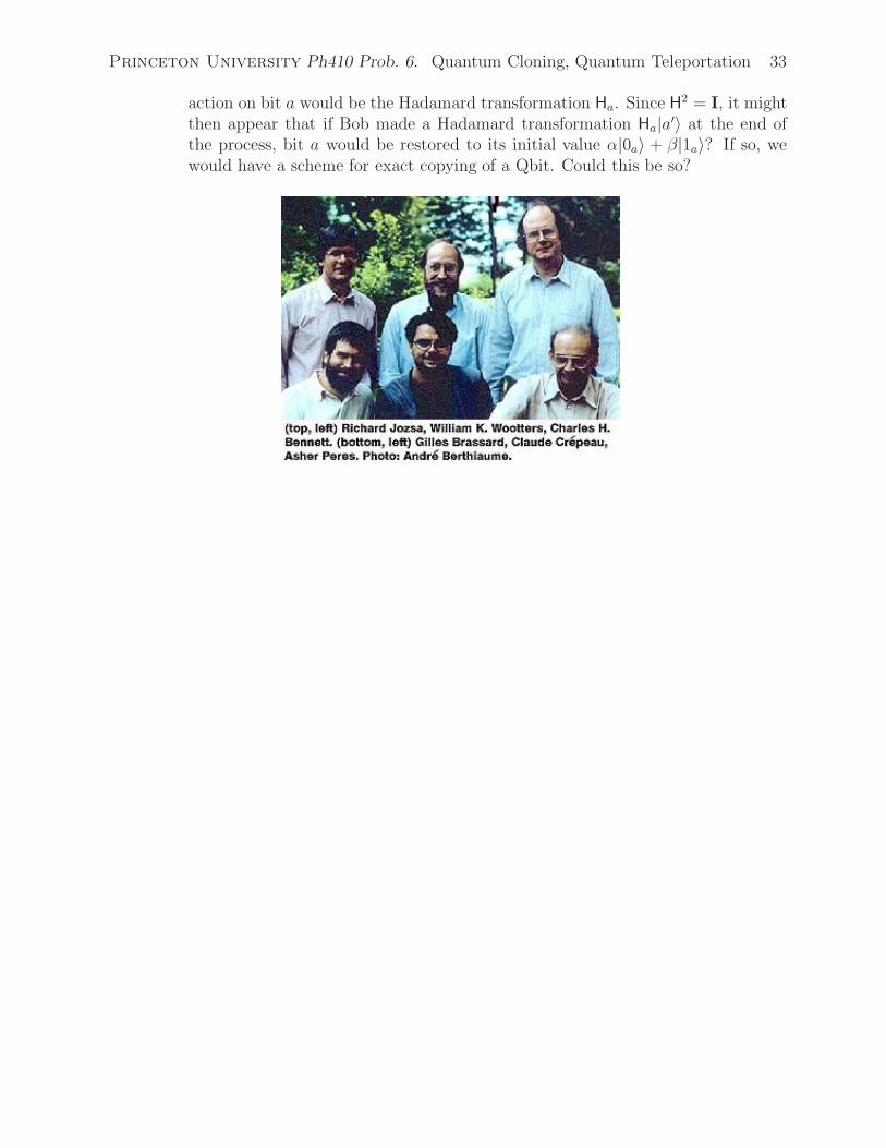
Princeton University Ph410 Prob. 6. Quantum Cloning, Quantum Teleportation 33
action on bit a would be the Hadamard transformation Ha. Since H2 = I, it mightthen appear that if Bob made a Hadamard transformation Ha|a′〉 at the end ofthe process, bit a would be restored to its initial value α|0a〉 + β|1a〉? If so, wewould have a scheme for exact copying of a Qbit. Could this be so?

Princeton University Ph410 Problem 7. Quantum Optics 34
7. Quantum Optics
A properly prepared quantum system can exhibit interference, which adds to the rich-ness of quantum computation. We illustrate this possibility with one or more photons indevices that contain various combinations of beam splitters, mirrors and phase-shiftingplates.
Dirac has written44 “Each photon then interferes only with itself. Interference betweentwo different photons never occurs.” Indeed, a practical definition is that “classical”optics consists of phenomena due to the interference of photons only with themselves.45
However, photons obey Bose statistics (which can be interpreted as a subtle kind ofinterference) which implies a “nonclassical” tendency for them to “bunch”.
(a) Phase Shift in a Lossless Beam Splitter
Give a classical argument based on a version of a Mach-Zehnder interferometer,as shown in the figure below, that there is a 90◦ phase shift between the reflectedand transmitted beams in a lossless, symmetric beam splitter. Then, followingDirac’s dictum, your result will apply to a single photon.
A beam of light of unit amplitude is incident on the interferometer from theupper left. The reflected and transmitted amplitudes are reiφr and teiφt , wherethe magnitudes r and t are real numbers. The condition of a lossless beam splitteris that
r2 + t2 = 1. (107)
The reflected and transmitted beams are reflected off mirrors and recombined ina second lossless beam splitter, identical to the first. The mirrors introduce anidentical phase changes φm into both beams, which can be ignored in the analysisof interference between the two beams. Deduce a relation between the phase shiftsφr and φt of the transmitted and reflected beams from the first splitter by notingthat the amplitudes A0 and A1 of the beams out of the second splitter also obey|A0|2 + |A1|2 = 1.
44P.A.M. Dirac, The Principles of Quantum Mechanics, 4th ed. (Clarendon Press, London, 1958), p. 9.45For early experimental evidence of single-photon interference, see
http://physics.princeton.edu/~mcdonald/examples/QM/taylor_pcps_15_114_09.pdf

Princeton University Ph410 Problem 7. Quantum Optics 35
This relation will have two-fold ambiguity. A more detailed analysis46 shows thatφr = φt + π/2. In our applications we can ignore the overall phase of the outputstate, and we will use this freedom to define φt = 0. Hence, we use φr = π/2 inthe following.
For the special case of 50:50 beam splitters in the interferometer, what are therelative intensities of output beams 1 and 2?
(b) Bunching of Photons in a Beam Splitter
As a simple example of nonclassical optical behavior, consider two photons of asingle frequency that are simultaneously incident on two sides of a lossless, 50:50beam splitter, as shown in the figure. Deduce the probability that N1 = 0, 1 or2 output photons are observed in the direction of beam 1. The key insight of aquantum analysis compared to a classical one is that photons obey Bose statistics,which means that the quantum probability that n indistinguishable photons arein a given state is n! times the probability that n distinguishable particles wouldbe in that state.47
Use the result of part (a) in your analysis, assuming that the two incident photonsare in phase (at the midplane of the beam splitter). Compare your calculation forphotons to a classical calculation for the output intensity on the two sides of thebeam splitter in the case of two input light beams of intensities i1 and i2 whichare not necessarily equal but which are in phase.
For use in part (e), deduce the probability, and probability amplitudes, for thefate of two in-phase photons that arrive simultaneously on opposite sides of alossless beam splitter for which the probability of reflection of a single photon isR = r2. The transmission probability is, of course, T = 1 − R.
(c) A Beam Splitter as a Quantum Processor
A beam splitter can be regarded as a processor of Qbits in which the |0〉 statecorresponds to the amplitude that a photon enters the splitter from one side, andthe |1〉 state corresponds to the amplitude that the same photon enters from theother side. [This is called spatial encoding, which can be arranged by sending asingle photon through a beam splitter prior to its arrival via two different pathsat the splitter of interest.]
46 See, for example, prob. 4(b) of http://physics.princeton.edu/~mcdonald/examples/ph501set6.pdf47See, for example, chap. 4, Vol. III of The Feynman Lectures on Physics (Addison-Wesley, 1965),
http://feynmanlectures.caltech.edu/III_04.html.

Princeton University Ph410 Problem 7. Quantum Optics 36
As shown in the figure below, label a photon that enters the splitter from theleft as |0〉 and one that enters from above as |1〉. The reflection coefficient of thesplitter is R = sin2 β
2.
Include up to four wave shifting plates at the entrance and exit ports of thesplitter, also shown in the figure above. If these plates have index of refractionn, how thick does one have to be to introduce a phase shift δ (in radians) for aphoton of wavelength λ?
What is the 2 × 2 unitary matrix U that describes the effect of the splitter (+wave shifting plates) on the general input state ψ0|0〉 + ψ1|1〉?Show that an arbitrary 2 × 2 unitary matrix, given by eqs. (44) and (56), can berepresented by a beam splitter and associated wave-shifting plates for appropriatechoices of the reflection coefficient and the phases φa, φb, φc and φd. Since a general2×2 unitary matrix is described by 4 parameters (that we call α, β, γ and δ), youshould find that one of the 4 phases φa, φb, φc and φd can be set to zero. Withthe convention that φa = 0, our optical realization of an arbitrary 2 × 2 unitarymatrix can also be drawn as
Thus, we have an example of how an arbitrary quantum transformation on a singleQbit can be accomplished with a passive system consisting of 4 (or 5, countingthe large mirror at the top of the second figure) pieces of glass.
Note that a beam splitter with reflection coefficient R = 1 is essentially a two-sided mirror. Such a mirror, without any phase-shifting plates, implements theNOT (= X) transformation by swapping the paths of input states |0〉 and |1〉, asshown on the next page.

Princeton University Ph410 Problem 7. Quantum Optics 37
Deduce the reflection coefficient R and the phase shifts φb, φc and φd needed toimplement the Z = σz gate and the Hadamard gate H. Present your results infigures such as that above.
(d) A Mach-Zehnder Interferometer as a Quantum Processor
Show that an arbitrary 2×2 unitary matrix can also be realized by a Mach-Zehnderinterferometer that uses lossless 50:50 beam splitters as well as 6 phase-shiftingplates, as shown in the figure below.
A photon that enters the interferometer from the left can be defined to be the|0〉 input state, while a photon that enters from the top can be called the |1〉input state. Similarly, we define a photon the emerges from the right of theinterferometer to be in the |0′〉 output state and one that emerges from the bottomto be in the |1′〉 output state. Inside the interferometer, a photon that moves tothe right and then down is said to be in the |0〉 state, while one that moves downand then to the right is said to be in the |1〉 state.
Deduce the form of a 2×2 unitary matrix M that describes the effect of a lossless50:50 beam splitter on the input photon state. Likewise, define unitary matricesφa, φb and φc that describe the effect of the 3 pairs of phase-shifting plates. Thenthe interferometer, when used with a single input photon, can be considered to

Princeton University Ph410 Problem 7. Quantum Optics 38
be a single-Qbit processor of the form
(e) An Optical Controlled-NOT Gate
Can beam splitters be used to implement 2-Qbit operations?
We explore this question by seeking an optical version of the Controlled-NOTgate, Cxy, that was introduced in problem 6(a). Recall that the effect of Cxy is toflip bit y if bit x is |1〉. The truth table for this operation is
Cxy :
x y x′ y′
0 0 0 0
0 1 0 1
1 0 1 1
1 1 1 0
(108)
A simple implementation of the Cxy operation is shown in the figure below, whichextrapolates from the construction of the NOT operation as discussed at the endof part (c). Again, only a single photon is used, but now that photon is “split”into 4 parts that are directed onto the incident paths labeled |00〉, |10〉, |01〉 and|11〉. A single beam splitter with reflection coefficient R = 1 swaps the paths ofinput states |01〉 and |11〉.
This is an example of a more general result that an arbitrary N×N unitary matrixcan be realized by a set of at most N(N − 1)/2 beam splitters and phase-shiftingplates, together with a single photon that is directed onto N input paths,48 assketched in the figure on the next page.
48 http://physics.princeton.edu/~mcdonald/examples/QM/reck_prl_73_58_94.pdfSee also, http://physics.princeton.edu/~mcdonald/examples/QM/cerf_pra_57_R1477_98.pdf
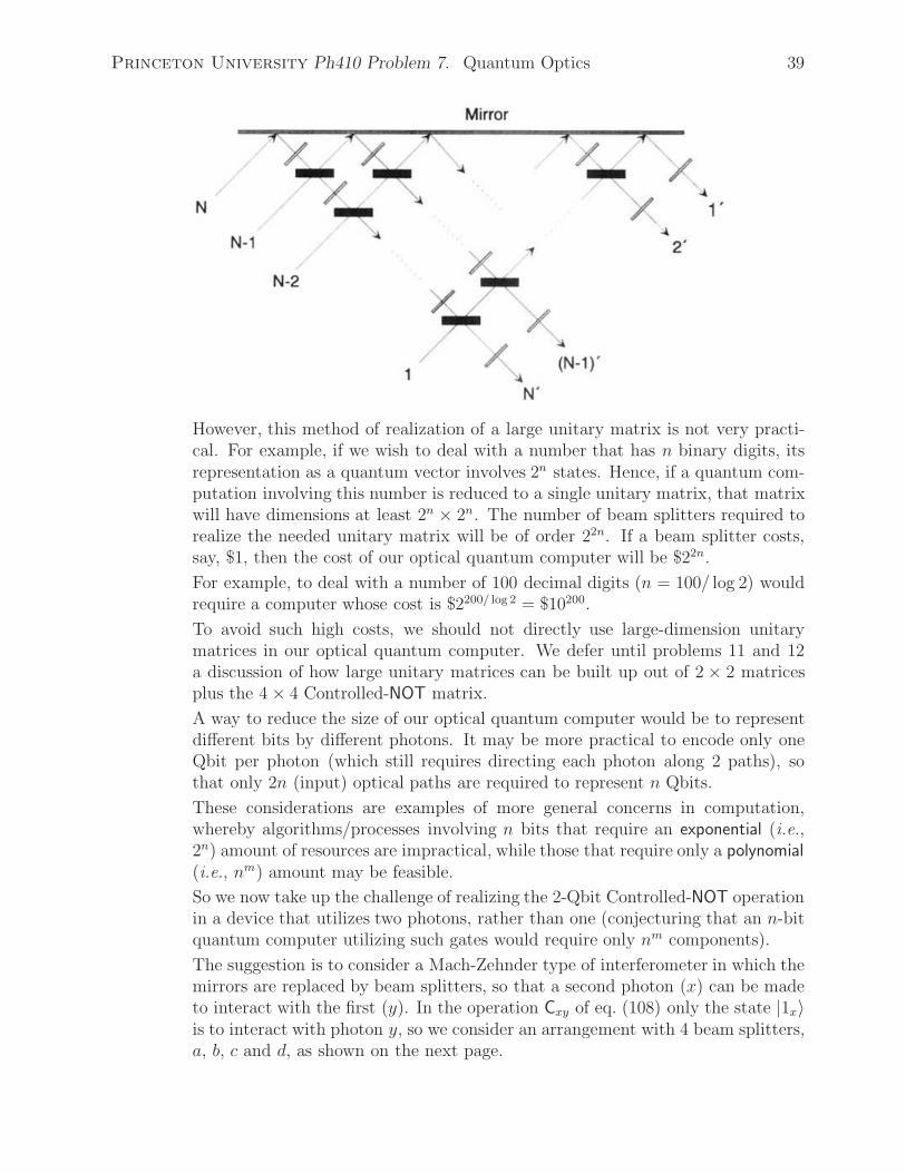
Princeton University Ph410 Problem 7. Quantum Optics 39
However, this method of realization of a large unitary matrix is not very practi-cal. For example, if we wish to deal with a number that has n binary digits, itsrepresentation as a quantum vector involves 2n states. Hence, if a quantum com-putation involving this number is reduced to a single unitary matrix, that matrixwill have dimensions at least 2n × 2n. The number of beam splitters required torealize the needed unitary matrix will be of order 22n. If a beam splitter costs,say, $1, then the cost of our optical quantum computer will be $22n.
For example, to deal with a number of 100 decimal digits (n = 100/ log 2) wouldrequire a computer whose cost is $2200/ log 2 = $10200.
To avoid such high costs, we should not directly use large-dimension unitarymatrices in our optical quantum computer. We defer until problems 11 and 12a discussion of how large unitary matrices can be built up out of 2 × 2 matricesplus the 4 × 4 Controlled-NOT matrix.
A way to reduce the size of our optical quantum computer would be to representdifferent bits by different photons. It may be more practical to encode only oneQbit per photon (which still requires directing each photon along 2 paths), sothat only 2n (input) optical paths are required to represent n Qbits.
These considerations are examples of more general concerns in computation,whereby algorithms/processes involving n bits that require an exponential (i.e.,2n) amount of resources are impractical, while those that require only a polynomial(i.e., nm) amount may be feasible.
So we now take up the challenge of realizing the 2-Qbit Controlled-NOT operationin a device that utilizes two photons, rather than one (conjecturing that an n-bitquantum computer utilizing such gates would require only nm components).
The suggestion is to consider a Mach-Zehnder type of interferometer in which themirrors are replaced by beam splitters, so that a second photon (x) can be madeto interact with the first (y). In the operation Cxy of eq. (108) only the state |1x〉is to interact with photon y, so we consider an arrangement with 4 beam splitters,a, b, c and d, as shown on the next page.

Princeton University Ph410 Problem 7. Quantum Optics 40
We immediately see that this scheme cannot represent the Controlled-NOT op-eration in all cases, because it can happen that photon y emerges at the unusedoutput, or photons x and y emerge in the states labeled |0′x〉 and |1′x〉, or in thestates |0′y〉 and |1′y〉, or both photons emerge in the state |1′x〉, etc.
However, we seek to show that when exactly one photon emerges in state |0′x〉or |1′x〉 and the other in |0′y〉 or |1′y〉, then the operation is the Controlled-NOT.This success occurs only part of the time, but the success can be identified by thepresence of exactly one final-state photon in the x′ states and exactly one in they′ states.
First, deduce the values of the reflection coefficients Ra, Rb, Rc and Rd of the 4beam splitters such that the two-photon initial state |0x〉|0y〉 cannot reach finalstate |0′x〉|1′y〉, and initial state |0x〉|1y〉 cannot reach final state |0′x〉|0′y〉. There ismore that one solution for this; it suffices to consider only the simplest. Verifythat the sum of the probabilities for all final states of the initial state |0x〉|0y〉 isunity.
Then, deduce additional constraints on the reflection coefficients such that thetwo-photon initial state |1x〉|0y〉 cannot reach final state |1′x〉|0′y〉 (and initial state|1x〉|1y〉 cannot reach final state |1′x〉|1′y〉).What fraction of the time does this interferometer function successfully as aControlled-NOT operation? Answer: Psuccess = 1/9.

Princeton University Ph410 Problem 8. Programmable Quantum Computer 41
8. A Programmable Quantum Computer?
In this problem you will show that there cannot be a completely general, programmablequantum computer, in contrast to the case for classical computation.
A classical n-to-n-bit function maps each of the 2n initial n-bit words, into one of 2n
possible final words. Such a function is completely specified by n2n bits. A generaln-bit classical computer (or programmable gate array) can be built that uses a list ofn2n bits (the program) to implement any desired function.
In quantum computation, the general n-bit function is described by an 2n×2n unitarymatrix U, which in turn can be described by 22n complex numbers subject to the 22n
constraints that U†U = I; i.e., a total of 22n independent real numbers define U. Sincea Qbit |ψ〉 = ψ0|0〉+ψ1|1〉 is described by 4−1 = 3 real numbers, it might seem that alist of 22n−1 Qbits could be sufficient to serve as the program of a general programmablequantum gate array to implement an arbitrary 2n × 2n unitary matrix U.
To this end, consider an m-Qbit program register |p〉 and an n-bit data register |d〉 ina direct-product state,
|p〉 ⊗ |d〉. (109)
Quantum operations on this state are described by (m+n)× (m+n) unitary matricesV. A programmable quantum gate array requires the operator V to obey
V[|pU〉 ⊗ |d〉] = |pU 〉 ⊗ U|d〉, (110)
where U is an arbitrary n × n unitary matrix, and |pU 〉 is the state of the programregister such that eq. (110) holds for each of the 2n data words |d〉.Consider two n× n unitary matrices Up and Uq and their associated program registerstates |p〉 and |q〉,
V[|p〉 ⊗ |d〉] = |p〉 ⊗ Up|d〉, (111)
V[|q〉 ⊗ |d〉] = |q〉 ⊗ Uq |d〉, (112)
to show that |p〉 and |q〉 are orthogonal whenever operators Up and Uq are distinct.
Hint: Take the scalar product of eqs. (111) and (112).
There are only 2m different orthogonal states in an m-Qbit register, but there are aninfinite number of different unitary matrices U. Hence, a finite-sized quantum gatearray can only be programmed for a small subset of possible quantum computations.
A consequence of this result is that the discussion of quantum computation in theremainder of this course will emphasize special-purpose quantum gate arrays, ratherthan programmable ones.

Princeton University Ph410 Problem 9. Designer Hamiltonians 42
9. Designer Hamiltonians
This problem is something of a historical digression on early visions of quantum com-putation.
One of the first motivations for consideration of quantum computers may have been thedesire for ever more compact processors, which leads us to contemplate processors onthe atomic scale. The realization by Bennett and Landauer that computation can beintrinsically reversible, except for erasure, encouraged Benioff49 to consider a spin-1/2lattice as the basis of a computer. Benioff only considered algorithms based on Cbits,but with a quantum implementation. A possible worry was that classical systems aresome kind of large-n limit of quantum systems, such that a quantum system mightnot successfully perform a “classical” algorithm. Benioff gave a formal argument thatHamiltonians for spin systems can be constructed such that the system behaves like aclassical processor.
A largely independent approach was taken by Feynman50 who appears to have beenmotivated by the challenge of computer simulation of quantum systems. For example,a system of n quantum subsystems which each have m states has a total of mn states.A single “cycle” of such a system has m2n possible transitions. Hence, a simulation ofeven a single cycle of this quantum system on a classical computer requires processingpower that is exponential in the size n of the system. Clearly a classical computer haslimited capability to simulate a quantum system. Perhaps a quantum computer wouldbe more appropriate for this task.
However, Feynman’s examples, like those of Benioff, were restricted to quantum im-plementation of classical algorithms. So, these early efforts served mainly to bringattention to the challenge of quantum computation.51
Both Benioff and Feynman emphasized the Hamiltonian of a quantum computer. Thisis, of course, inspired by Schrodinger’s equation for the time development of a quantumstate |ψ〉,
ih∂
∂t|ψ(t)〉 = H(t)|ψ〉 = hh(t)|ψ〉, (113)
where H(t) is not the Hadamard transformation but is the Hamiltonian operator. Aformal solution for the time dependence of state |ψ〉 is then
|ψ(t)〉 = e−i∫
h(t)dt|ψ(0)〉 = U(t)|ψ(0)〉. (114)
49 http://physics.princeton.edu/~mcdonald/examples/QM/benioff_prl_48_1581_82.pdf50 Chap. 6 of Feynman Lectures on Computation (Addison-Wesley, 1996), which was written in 1985.
http://physics.princeton.edu/~mcdonald/examples/QM/feynman_computation_chap6.pdfSee also http://physics.princeton.edu/~mcdonald/examples/QM/feynman_fp_16_507_86.pdfThe challenge of simulation of quantum systems by other quantum systems was identified in the ’70’s byPoplavskii and by Manin,http://physics.princeton.edu/~mcdonald/examples/QM/manin_quant-ph-9903008.pdf
51 Somewhat surprisingly, Feynman wrote (p. 185 of the book cited above) that as to the question of thelimitations to computing due to quantum mechanics and the uncertainty principle, “I have found that, asidefrom the obvious limitation to size if the working parts are to be made of atoms, there is no fundamentallimits from these sources.”

Princeton University Ph410 Problem 9. Designer Hamiltonians 43
In case the Hamiltonian is time independent, as will be considered below, the timeevolution becomes more simply
|ψ(t)〉 = e−iht|ψ(0)〉. (115)
The meaning of the formal expression (115) is clarified by making the Taylor expansion,
e−iht =∞∑n=0
(−iht)nn!
= I − iht− h2t2
2+ih3t3
6+ · · · (116)
A way of thinking about this expansion is that during the time evolution of the state|ψ〉 the Hamiltonian operator is applied over and over in groups of various numbers n ofrepetitions (products of h), with the set of n repetitions being weighted by (−it)n/n!.
Feynman addressed the task of finding a Hamiltonian h that implements a (reversible)quantum computation that is described by a unitary matrix M. That is, the desiredcomputation is |ψ′〉 = M|ψ〉. In general, the computation is built up out of a sequenceof m steps, each of which is described by a unitary matrix Mj . Then, the overallcomputation is represented by the product of the Mj
M =m∏j=1
Mj = MmMm−1 · · ·M2M1. (117)
The computation involves, say, n Qbits, so that the matrices Mj are of size 2n × 2n.
If a Hamiltonian can be constructed so that its jth application executes operator Mj,then a group of m repetitions of this Hamiltonian would correspond to the desiredcomputation. The time evolution operator (116) would include this action, amongothers. The remaining task would be to make some kind of measurement on the state|ψ(t)〉 that reveals the result of the computation.
Feynman increased the working size of the system to m+n+1 Qbits. He described then Qbits on which the computation M is made as the data register, and the additionalm + 1 Qbits as the program counter.52 The goal is to have the program counter in areadily identifiable state when the quantum computation has been completed.
Annihilation and Creation Operators.
To play with the Qbits in the program counter it is useful to introduce matrices thatserve as annihilation and creation operators. The annihilation operator a for a singleQbit is defined as
a =
⎛⎝ 0 1
0 0
⎞⎠ (annihilation). (118)
Its action on |1〉 is to turn it into |0〉, while it takes |0〉 to the “|vacuum〉” state,
a|1〉 =
⎛⎝ 0 1
0 0
⎞⎠⎛⎝ 0
1
⎞⎠ =
⎛⎝ 1
0
⎞⎠ = |0〉, a|0〉 =
⎛⎝ 0 1
0 0
⎞⎠⎛⎝ 1
0
⎞⎠ =
⎛⎝ 0
0
⎞⎠ = |vac〉, (119)
52Feynman’s quantum computer illustrates the result of prob. 8 that a program register of (at least) mbits is needed to program a computation that involves m different unitary operations.

Princeton University Ph410 Problem 9. Designer Hamiltonians 44
It is conventional to say that the effect of the annihilation operator on the |0〉 state isto return the number 0:
a|0〉 = 0|0〉. (120)
The hermitian conjugate (adjoint) of the annihilation operator a is the creation oper-ator a†,
a† =
⎛⎝ 0 0
1 0
⎞⎠ (creation), (121)
a†|0〉 =
⎛⎝ 0 0
1 0
⎞⎠⎛⎝ 1
0
⎞⎠ =
⎛⎝ 0
1
⎞⎠ = |1〉, a†|1〉 =
⎛⎝ 0 0
1 0
⎞⎠⎛⎝ 0
1
⎞⎠ =
⎛⎝ 0
0
⎞⎠ = 0.
(122)The product a†a is
a†a =
⎛⎝ 0 0
1 0
⎞⎠⎛⎝ 0 1
0 0
⎞⎠ =
⎛⎝ 0 0
0 1
⎞⎠ ≡ n, (123)
where n is the number operator,
n|1〉 = 1|1〉, n|0〉 = 0|0〉, (124)
according to the convention (120). The product aa† is
aa† =
⎛⎝ 0 1
0 0
⎞⎠⎛⎝ 0 0
1 0
⎞⎠ =
⎛⎝ 1 0
0 0
⎞⎠ = I − n ≡ n, (125)
and clearlyaa† + a†a = I. (126)
Any 2× 2 matrix can be built up out of linear combinations of a, a†, aa† and a†a, i.e.,out of sums and products of a and a†. For example, the other classical unitary 2 × 2matrix, X (NOT), can be written as
X = a + a†. (127)
(a) Express the Controlled-NOT operator Cab (that flips bit b if bit a = |1〉) in termsof the annihilation and creation operators a and a† for bit a and b and b† for bitb. Use a tensor product notation.
(b) Express the Controlled-Controlled-NOT operator (also called the Toffoli gate) Cabc(that flips bit c only if both bits a and b are |1〉) in terms of the annihilation andcreation operators a, a†, b, b†, c and c†. Your result should show the symmetryof Cabc with respect to bits a and b. For compactness, you need not expand unitmatrices in terms of annihilation and creation operators. What is the 8×8 unitarymatrix representation of the Toffoli gate?

Princeton University Ph410 Problem 9. Designer Hamiltonians 45
Feynman suggests that we construct a time-independent Hamiltonian h based on them unitary operations Mj with the aid of the annihilation and creation operators pkand p†
k for the m+ 1 program counter bits according to
h =m−1∑j=0
p†j+1 ⊗ pj ⊗ Mj+1 + pj+1 ⊗ p†
j ⊗ M†j+1. (128)
The presence of the hermitian conjugate of each term insures that the Hamiltonianis hermitian even though each term of the sum is not. The tensor product notationreminds us that the three factors of each term operate on different bits in our workingspace of m+ n + 1 bits.
This Hamiltonian is designed such that only one of the program counter bits is nonzeroat any time.
For example, if all the program counter bits are |0〉, then the h acting on this systemproduces 0, since every term of eq. (128) contains an annihilation operator.
And, if exactly one program counter bit is equal to |1〉, say bit k (and the others are all|0〉), then only the term p†
k+1 ⊗pk⊗Mk+1 among the terms containing the Mj producesa nonzero result which is to flip bit k to |0〉, flip bit k + 1 to |1〉 and apply operationMk+1 to the n data-register bits. The final result still has exactly one of the programcounter bits equal to |1〉.We see that for the program counter bit k to have been |1〉 the last previous operationon the register bits must have been Mk, which occured when program counter bitk − 1 was |1〉. By induction, after the Hamiltonian has operated when bit k is |1〉 theregister has been subject to the sequence of operations Mk+1Mk · · ·M1. Thus, repeatedapplications of the Hamiltonian increment the position of the nonzero program counterbit, and build up the computation on the register.
Once program-counter bit m+1 has been set to |1〉 (and all the other program-counterbits are |0〉), further applications of the terms of the Hamiltonian that contain the Mj
make no changes to the system.
However, the Hamiltonian h also includes the term pk ⊗ p†k−1 ⊗ M†
k, which is neededfor h to be hermitian. So if program counter bit k is |1〉, this term sets bit k back to|0〉, sets bit k − 1 to |1〉 and applies operator M†
k to the register. Now, for bit k tohave been |1〉 the last previous operation on the register must have been Mk. So thecombined action of the last two operations on the register is M†
kMk = I. This bringsthe register back to the state after operator Mk−1 was applied to it. In brief, the effectof the term pk ⊗ p†
k−1 ⊗M†k is simply to set the computation back one step.
Since the Hamiltonian contains the sum of operators p†k+1⊗pk⊗Mk+1 and pk⊗p†
k−1⊗M†k,
the register ends up in a quantum superposition of the computation up through thek + 1st step and the k − 1st step.
Indeed, after the Hamiltonian has been applied to the system a large number of times,the system is in a quantum superposition of all intermediate states of the system,including the final state that contains the desired answer to the computation.
To extract a result, we observe the state of program-counter bit m+1. If it is found tobe |0〉, we were unlucky in projecting out one of the components of the quantum state

Princeton University Ph410 Problem 9. Designer Hamiltonians 46
that did not correspond to a completed computation. But if we find program-counterbit m+1 to be |1〉, then we have observed the system in a state of completion, and wecan look at the register bit to obtain the result of the computation.
Feynman’s quantum computer therefore proceeds as follows:
• Construct the Hamiltonian h for the computation M according to eq. (128), andconstruct the time-evolution operator (116) from this.
• Initialize the program-counter bits to |0〉, except for the first counter bit, whichis set to |1〉. Initialize the data-register bits as appropriate. This defines thequantum state |ψ(0)〉.
• Apply the time evolution operator (116) to the initial state |ψ(0)〉.• Observe program-counter bit m+ 1 at suitable time intervals until it is found to
have a value of |1〉. Then observe the data-register bits to read off the result ofthe computation.
A classical computer simulation of the quantum computation of a classical one-bitcomputation of the NOT operator is available as a Mathematica .nb file,http://physics.princeton.edu/~mcdonald/examples/QM/Williams/WINDOWS/NBOOKS3/FEYNMAN.
NB for Windows PC’s. Versions for MAC and Linux are available in related directories.53
This notebook is a tutorial about constructing and running a simulation of a Feynmanquantum computer for the computation NOT =
√NOT ·√NOT. The register contains
only a single bit, and the program counter contains 2 + 1 bits, since the computation isactually made in 2 steps. The computer requires a total of 4 Qbits, so the Hamiltonianand the time-evolution operator are 16 × 16 matrices.
Work through the tutorial at your leisure. Then complete exercises (c)-(h), using the.nb file as you find convenient.
Do these exercises in the spirit of Benioff and Feynman, i.e., use only classical unitaryoperators to perform the computations themselves. In particular, use only the NOT,the Controlled-NOT, and the Controlled-Controlled-NOT operators, which are imple-mented in the .nb file as NOTGate[i,m], CNGate[i,j,m], and CCNGate[i,j,k,m],respectively. Index m describes the total number of bits in the register, while bits i,j and k indicate which bits are acted upon by a particular gate. The bits i, j and k
need not be in sequential order.
Although the exercises involve the construction of classical gates, this is to be donewith quantum gates that can function on arbitrary Qbits. Remember that an arbitraryQbit cannot be cloned, but a Controlled-NOT gate can be used to make a copy of aCbit state.
For each exercise, provide a diagram of your circuit, and use the .nb file to presentthe TruthTable for the circuit. The circuits may involve some bits that are initializedto zero. Include only those lines of output from the TruthTable in which those bits
53 To initialize the notebook, place the cursor to the right of the first executable command,Off[General::spell1], and press Shift-Enter rather than merely Enter. Answer YES to the initializa-tion popup window. To execute any of the other commands in the notebook, also press Shift-Enter afterplacing to cursor to the right of that command.

Princeton University Ph410 Problem 9. Designer Hamiltonians 47
are initially zero. If your circuit involves a sequence of gates, say, G1G2G3, note thatTruthTable[G3 . G2 . G1] is not the same as TruthTable[G1 . G2 . G3].
We defer until problem 11 the question of whether the following operations could beimplemented using only 1-bit and 2-bit gates.
(c) Construct the AND gate for 2 Cbits, which is equivalent to constructing a gatethat multiplies two Cbits. Devise a measurement operator M to observe theoutput bit. What is the effect of the multiplier circuit on general input Qbits|a〉 = a0|0〉+ a1|1〉 and |b〉 = b0|0〉 + b1|1〉 as inferred from the measurement? Forexample, what are the probabilities that the output bit is 0 or 1?
(d) Construct the OR gate for 2 Cbits.
(e) Construct a circuit that adds two Cbits. The simplest circuit to do this willinvolve one ancillary bit. Since the sum of two bits is a two-bit number, one ofthe initial bits will be overwritten by the simplest circuit. Also construct a circuitwith two ancillary bits that adds two Cbits, leaving these input bits unaltered.
Explore the effect of your circuits on general initial Qbits. Devise a measurementoperator A to observe the two output bits. What are the probabilities that thesebits corresponds to the sum being 0, 1 or 10? Note that the effect of your addercircuits on Qbits is not the same as the addition of Qbits as vectors. Note alsothat the result of a measurement of the output sum of your two circuits is in effectthe same, even though it is not possible to clone an arbitrary Qbit in the sensediscussed in problem 6. Hence, the no-cloning theorem is not quite as restrictivefor quantum computation as it may have first appeared.
(f) Construct a circuit that adds three Cbits. This circuit will be needed for “car-rying” during the addition of two multiple-bit numbers. In a particularly simplecircuit, one of the two bits of the sum overwrites, say, the third input bit.
Hint: Since bit c is to be overwritten, start with a circuit that adds bits b and c,and append one that adds bits a and c.
(g) Construct a circuit that adds two 2-Cbit numbers a and b, overwriting b in theprocess.
It would be good to have a circuit that could be generalized to add two n-Cbitnumbers. The circuit from part (f) can be an ingredient if we consider bit ato be the “carry” bit from the previous addition(s) of the lower-order bits ofa =
∑j=0 aj2
j and b =∑j=0 bj2
j .54 The high-order output bit d then becomesthe “carry” bit for the subsequent addition(s) of higher-order bits of a and b.
54In decomposing an n-bit binary number as a =∑n−1
j=0 aj2j, we indicate the lowest-order bit as a0 andthe highest-order bit at an−1. Unfortunately, many authors, including Nielsen and Chuang, use a reverseconvention in which a1 is the highest-order bit and an is the lowest-order bit: a =
∑nj=1 aj2n−j.

Princeton University Ph410 Problem 9. Designer Hamiltonians 48
The “obvious” solution has the defect that at the end of the addition, the “carry”lines may not be in their initial |0〉 states, which would prevent the circuit frombeing reused to perform other additions. Therefore, it is more elegant to augmentthe “obvious” solution with a group of gates that undoes the calculation of thelower-order “carry” bit(s), without changing the state of the b bits (which containthe sum a + b). Show that a minor variation of the circuit of part (f) does thisjob.
The hints are encouraging you to build a kind of “ripple adder”, which usesroughly 3n bits to add two n-bit numbers. The tacit assumption is that in aquantum computer bits are expensive, but speed is not an issue. The converse istrue in classical computation today, and addition is typically done by “carry-save”circuits that require of order n2 bits to add two n-bit numbers.
(h) Construct a circuit that multiplies two 2-Cbit numbers.
Again, minimize the number of bits required, and restore any ancillary bits totheir initial state.
Multiplication requires lots of bits. If bits are expensive in a quantum computer,it will be preferable to perform algorithms that multiply n-bit numbers moduloN , where N < n, since in this case the product is at most n bits long. As we willsee in prob. 17, one of the most important algorithms in quantum computationis of this type.
Besides the artificial restriction by Feynman that his computer use only classical gatesfor the computation itself, it is also overly constrictive to embed a unitary computationM inside the Hamiltonian (128) that runs the computation forwards and backwards ina probabilistic manner. If we can actually implement the computation M in suitablehardware, it will be more efficient simply to apply M once, directly to the data-registerstate |ψd〉 to obtain the result |ψ‘d〉 = M|ψd〉.As Feynman stated, his computer was designed more to draw attention to the option ofperforming computations with quantum-scale devices that to indicate how this mightbest be done.55
55An early review of the quantum computers of Benioff and Feynman is given inhttp://physics.princeton.edu/~mcdonald/examples/QM/peres_pra_32_3266_85.pdf

Princeton University Ph410 Problem 10. Deutsch’s Algorithm 49
10. Deutsch’s Algorithm
The first example of a quantum computation that could have a speed advantage overthe corresponding classical version was given by Deutsch in 1985.56
A single classical processor can only evaluate a function of a single variable for onevalue of that variable at a time. In contrast a quantum processor that can evaluate afunction for a general quantum state, i.e., a superposition of orthogonal states, obtainsinformation about that function for all orthogonal states during a single evaluation. Inan important sense, a quantum processor is intrinsically a parallel processor.
To maximize the information that can be obtained from a single evaluation of f(x) fora Qbit |x〉, we choose that Qbit to be a mixture of bits |0〉 and |1〉, namely
|x〉 = |+〉 =|0〉 + |1〉√
2= H|0〉, (129)
where H is the Hadamard transformation introduced in eq. (60).
This trick can be generalized to the case of functions of n Qbits by applying the n-fold tensor product of Hadamard transformations to the 0 state of n Qbits, |0〉n =|000 . . . 0〉,
H⊗n|0〉n = H ⊗H ⊗ · · · ⊗H|000 . . . 0〉 = H|0〉H|0〉 · · ·H|0〉=
|0〉 + |1〉√2
|0〉 + |1〉√2
· · · |0〉 + |1〉√2
=1
2n/2(|000...00〉 + |000...01〉 + |000...10〉 + . . . + |111...11〉)
=1
2n/2(|0〉n + |1〉n + |2〉n + . . .+ |2n − 1〉n)
=1
2n/2
2n−1∑j=0
|j〉n. (130)
The state (130) is still a direct product (∏n−1l=0 |+l〉), but any subsequent operation on
this state that does not affect all Qbits identically will result in an entangled state.
A single evaluation of a function f for the quantum state (130) will contain informationas to all of the values f(|j〉n), which is touted by Deutsch as “quantum parallelism”.
Of course, to learn about the result we must make a measurement, which will projectthe state f(H⊗n|0〉n) onto a single real number whose relation to the f(|j〉n) will notbe known. Only with additional cleverness will it be advantageous to use a quantumprocessor.
Deutsch illustrated this for a function f of a single bit. Classically, there are only fourpossibilities for the function f :
56 http://physics.princeton.edu/~mcdonald/examples/QM/deutsch_prsl_a400_97_85.pdfhttp://physics.princeton.edu/~mcdonald/examples/QM/deutsch_prsl_a439_553_92.pdfhttp://physics.princeton.edu/~mcdonald/examples/QM/cleve_ptrsl_454_339_98.pdfOnline lectures by Deutsch: http://cam.qubit.org/video_lectures/index.php
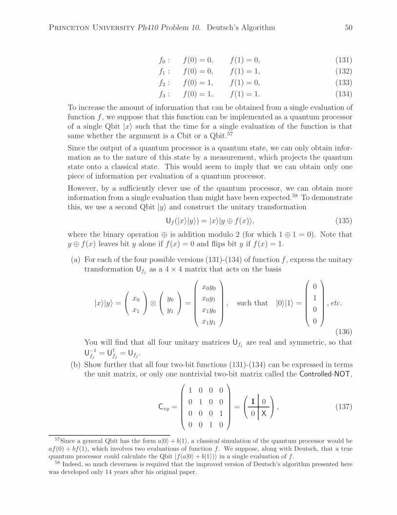
Princeton University Ph410 Problem 10. Deutsch’s Algorithm 50
f0 : f(0) = 0, f(1) = 0, (131)
f1 : f(0) = 0, f(1) = 1, (132)
f2 : f(0) = 1, f(1) = 0, (133)
f3 : f(0) = 1, f(1) = 1. (134)
To increase the amount of information that can be obtained from a single evaluation offunction f , we suppose that this function can be implemented as a quantum processorof a single Qbit |x〉 such that the time for a single evaluation of the function is thatsame whether the argument is a Cbit or a Qbit.57
Since the output of a quantum processor is a quantum state, we can only obtain infor-mation as to the nature of this state by a measurement, which projects the quantumstate onto a classical state. This would seem to imply that we can obtain only onepiece of information per evaluation of a quantum processor.
However, by a sufficiently clever use of the quantum processor, we can obtain moreinformation from a single evaluation than might have been expected.58 To demonstratethis, we use a second Qbit |y〉 and construct the unitary transformation
Uf (|x〉|y〉) = |x〉|y ⊕ f(x)〉, (135)
where the binary operation ⊕ is addition modulo 2 (for which 1 ⊕ 1 = 0). Note thaty ⊕ f(x) leaves bit y alone if f(x) = 0 and flips bit y if f(x) = 1.
(a) For each of the four possible versions (131)-(134) of function f , express the unitarytransformation Ufj as a 4 × 4 matrix that acts on the basis
|x〉|y〉 =
⎛⎝ x0
x1
⎞⎠⊗
⎛⎝ y0
y1
⎞⎠ =
⎛⎜⎜⎜⎜⎜⎜⎝
x0y0
x0y1
x1y0
x1y1
⎞⎟⎟⎟⎟⎟⎟⎠, such that |0〉|1〉 =
⎛⎜⎜⎜⎜⎜⎜⎝
0
1
0
0
⎞⎟⎟⎟⎟⎟⎟⎠, etc.
(136)
You will find that all four unitary matrices Ufj are real and symmetric, so that
U−1fj
= U†fj
= Ufj .
(b) Show further that all four two-bit functions (131)-(134) can be expressed in termsthe unit matrix, or only one nontrivial two-bit matrix called the Controlled-NOT,
Cxy =
⎛⎜⎜⎜⎜⎜⎜⎝
1 0 0 0
0 1 0 0
0 0 0 1
0 0 1 0
⎞⎟⎟⎟⎟⎟⎟⎠
=
⎛⎝ I 0
0 X
⎞⎠ , (137)
57Since a general Qbit has the form a|0〉 + b|1〉, a classical simulation of the quantum processor would beaf(0) + bf(1), which involves two evaluations of function f . We suppose, along with Deutsch, that a truequantum processor could calculate the Qbit |f(a|0〉 + b|1〉)〉 in a single evaluation of f .
58 Indeed, so much cleverness is required that the improved version of Deutsch’s algorithm presented herewas developed only 14 years after his original paper.
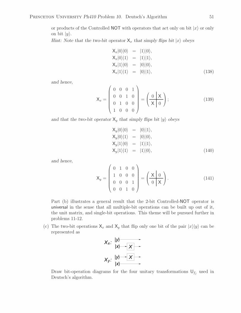
Princeton University Ph410 Problem 10. Deutsch’s Algorithm 51
or products of the Controlled NOT with operators that act only on bit |x〉 or onlyon bit |y〉.Hint: Note that the two-bit operator Xx that simply flips bit |x〉 obeys
Xx|0〉|0〉 = |1〉|0〉,Xx|0〉|1〉 = |1〉|1〉,Xx|1〉|0〉 = |0〉|0〉,Xx|1〉|1〉 = |0〉|1〉, (138)
and hence,
Xx =
⎛⎜⎜⎜⎜⎜⎜⎝
0 0 0 1
0 0 1 0
0 1 0 0
1 0 0 0
⎞⎟⎟⎟⎟⎟⎟⎠
=
⎛⎝ 0 X
X 0
⎞⎠ ; (139)
and that the two-bit operator Xy that simply flips bit |y〉 obeys
Xy|0〉|0〉 = |0〉|1〉,Xy|0〉|1〉 = |0〉|0〉,Xy|1〉|0〉 = |1〉|1〉,Xy|1〉|1〉 = |1〉|0〉, (140)
and hence,
Xy =
⎛⎜⎜⎜⎜⎜⎜⎝
0 1 0 0
1 0 0 0
0 0 0 1
0 0 1 0
⎞⎟⎟⎟⎟⎟⎟⎠
=
⎛⎝ X 0
0 X
⎞⎠ . (141)
Part (b) illustrates a general result that the 2-bit Controlled-NOT operator isuniversal in the sense that all multiple-bit operations can be built up out of it,the unit matrix, and single-bit operations. This theme will be pursued further inproblems 11-12.
(c) The two-bit operations Xx and Xy that flip only one bit of the pair |x〉|y〉 can berepresented as
Draw bit-operation diagrams for the four unitary transformations Ufj used inDeutsch’s algorithm.

Princeton University Ph410 Problem 10. Deutsch’s Algorithm 52
Suppose we implement Deutsch’s algorithm with |y〉 = (|0〉− |1〉)/√2 = H|1〉 = HX|0〉.Then we have
|y ⊕ f(x)〉 =|0 ⊕ f(x)〉 − |1 ⊕ f(x)〉√
2= (−1)f(x) |0〉 − |1〉√
2= (−1)f(x)|y〉. (142)
This is a remarkable trick, whereby the state |y〉 is unchanged except for a phase factorthat depends on the value of f(x).
The trick can be exploited by choosing state |x〉 to be H|0〉 = (|0〉 + |1〉)/√2. Then,
|x〉|y ⊕ f(x)〉 =(−1)f(0)|0〉 + (−1)f(1)|1〉√
2
|0〉 − |1〉√2
. (143)
Another remarkable thing has happened here. The phase factor that appeared ineq. (142) is now a shared property of the direct product state |x〉|y⊕ f(x)〉 = Uf |x〉|y〉.And since the state of |y〉 did not change for the particular case that |y〉 = HX|0〉, thisphase factor is now more a property of the state |x〉 than of |y〉. Yet, the operatorUf ostensibly did not change |x〉. This is one of the features that will permit (some)quantum computations to be more efficient than their classical versions.
To learn about the state (143) we don’t need to measure the second bit since it isunchanged from its initial value of (|0〉 − |1〉)/√2. So, we only measure the first bit.It is advantageous to measure this bit in the basis |±〉 = (|0〉 ± |1〉)/√2, which leadsto the result
|x〉 =
⎧⎪⎨⎪⎩
|+〉, if f(0) = f(1),
|−〉, if f(0) = f(1).(144)
While we have not learned both the values f(0) and f(1) from a single measurement,we have learned whether or not f(0) equals f(1). To obtain the latter knowledge bya classical computation would require two evaluations of function f , whereas we havelearned this from a single quantum evaluation of f .
(d) If the transformation (135) is used with classical bits, the first bit would beunchanged and in general the second bit would be changed. Note that whenwe applied this transformation to a particular set of quantum bits, the first bitwas changed in general, while the second bit was not. Clearly the behavior of aquantum processor is more subtle than that of a classical processor.
According to Bennett, it should be possible to reverse the quantum computationand restore the bits to their initial states. For the particular set of initial bits,|x〉 = |+〉 and |y〉 = |−〉, what is the procedure to restore these bits followingapplication of transformation (135) and the measurement of the first bit?
(e) Suppose we prefer to measure in the [|0〉, |1〉] basis rather than in the [|+〉, |−〉]basis as was done for the state (143). Devise a (simple) unitary transformationof state (143) such that measurement in the [|0〉, |1〉] tells us whether f(0) = f(1)or not. Draw a diagram of the revised process, with input states |x〉 = |y〉 = 0.You may indicate the transformation Uf by the symbol

Princeton University Ph410 Problem 10. Deutsch’s Algorithm 53
(f) The Deutsch-Jozsa Algorithm.
Design a circuit that generalizes Deutsch’s algorithm to address the somewhatacademic problem of determining whether a 1-bit function f(x), where x consistsof n bits, is balanced or constant when all we know about f is that it is one ofthese two types. The classical version of function f returns only 0 or 1. Thefunction is balanced if it is 0 for exactly half of all values of x and 1 for the otherhalf. And of course, the function is constant if it is either 0 for all values of x or1 for all values.
Hint 1: The spirit of this part is to make the “obvious” generalization of Deutsch’salgorithm for an n-to-1 bit function, and then to figure out what problem thisalgorithm solves.
Hint 2: Demonstrate that eq. (130) may be generalized as
H⊗n|j〉n =1
2n/2
2n−1∑k=0
(−1)j�k|k〉n, (145)
where |j〉n and |k〉n are n-bit, direct-product basis states as in eq. (16), andj � k =
∑l jlkl (mod 2) is the scalar product of j and k, modulo 2, when they are
considered to be n-dimensional vectors whose elements are only 0’s and 1’s.

Princeton University Ph410 Problem 11. Universal Classical Gates 54
11. Universal Gates for Classical Computation
Classical computations are built up from computations on pairs of Cbits. A basicclassical gate has two Cbits as input and one Cbit as output. The truth table for sucha gate has 4 entries, corresponding to the input bits having values (0,0), (0,1), (1,0)and (1,1). Since the output bit can take on two values, 0 and 1, there are 24 = 16different classical 2-bit gates. The historical name for 2-bit classical gates (logic gates)is Boolean functions.59
Symbols and truth tables for several 2-bit classical gates are shown below.
The question arises as to whether some subset of the 16 2-bit classical gates are universalin the sense that the remaining gates (and hence all classical computations) can beconstructed from products of the universal gates.
It turns out that there are 19 different minimal sets of universal 2-bit classical gates.Two of these sets contain only a single gate, 7 contains two gates, and 12 contain threegates. The NAND and NOR gates are each universal for classical computation.
59An entertaining survey of classical computation is The New Turing Omnibus by A.K. Dewdney (Com-puter Science Press, New York, 1993).

Princeton University Ph410 Problem 11. Universal Classical Gates 55
Technical aside: The 1-bit NOT gate and the 2-bit NAND gate are particularly simpleto implement with transistors, and so have a favored status. The figure below sketchesimplementations of these gates with one and two transistors, respectively.
Bits a and b are implemented by voltages with bit value 0 given by 0 volts, and bit value1 given by a positive voltage large enough to make the transistor conduct when appliedto the gate (= base). Thus in the NOT circuit, the output voltage is high when theinput voltage is low, and vice versa. Similarly, in the NAND circuit the output voltageis high unless both input voltages are high.
(a) The 2-Bit NAND Gate is Universal for Classical Computation.
Illustrate the classical universality of the 2-bit NAND gate by showing how to useit to implement the AND, OR and NOT gates. If you will accept that the latterthree gates form a universal set, you have then shown that the NAND gate aloneis universal. (Otherwise, show that the remaining 11 2-bit classical gates can alsobe implemented via NAND gates.)
(b) The Controlled-Controlled-NOT Gate is Universal for Classical Com-putation.
Turning now to implementations of computation via quantum gates, we recallthat these gates must be unitary (and so have the same number of outputs asinputs). We have seen in Prob. 9 that the Controlled-Controlled-NOT is usefulin implementing various computational functions. Show that this 3-bit gate isuniversal for classical computations by implementing the 2-bit NAND gate withit.
If we add the requirement for quantum circuits that any ancillary bits must havetheir initial state as |0〉, then we must relax our definition of classical universalityof a quantum gate to mean that it, together with any needed 1-bit quantum gates,suffices to implement any classical computation.
See sec. 6.1.3 of Preskill’s lecture notes for a discussion of how an arbitrary n-Cbittransformation can be built up out of Controlled-Controlled-NOT gates.
(c) The Controlled-NOT Gate is Universal for Classical Computation.
A 3-bit quantum gate requires the coupling of three input Qbits, which is muchmore difficult than coupling only two Qbits. Hence, it is advantageous if there isa set of 2-bit quantum gates that is universal for classical computation.
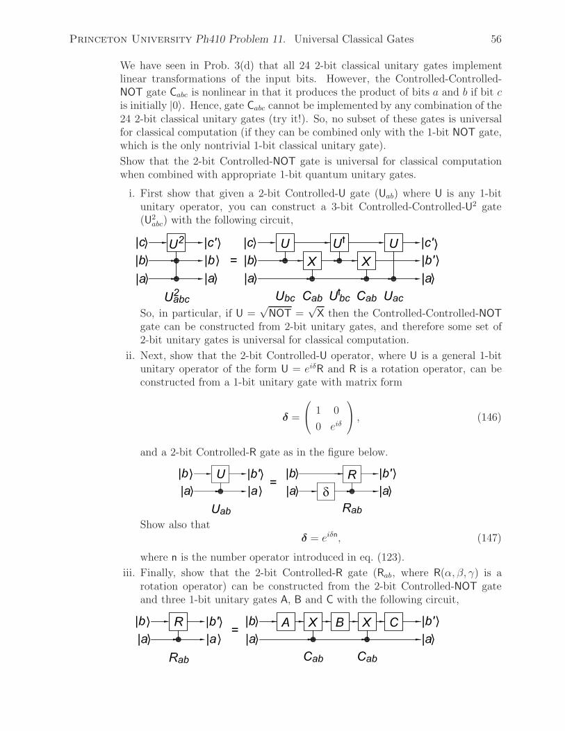
Princeton University Ph410 Problem 11. Universal Classical Gates 56
We have seen in Prob. 3(d) that all 24 2-bit classical unitary gates implementlinear transformations of the input bits. However, the Controlled-Controlled-NOT gate Cabc is nonlinear in that it produces the product of bits a and b if bit cis initially |0〉. Hence, gate Cabc cannot be implemented by any combination of the24 2-bit classical unitary gates (try it!). So, no subset of these gates is universalfor classical computation (if they can be combined only with the 1-bit NOT gate,which is the only nontrivial 1-bit classical unitary gate).
Show that the 2-bit Controlled-NOT gate is universal for classical computationwhen combined with appropriate 1-bit quantum unitary gates.
i. First show that given a 2-bit Controlled-U gate (Uab) where U is any 1-bitunitary operator, you can construct a 3-bit Controlled-Controlled-U2 gate(U2
abc) with the following circuit,
So, in particular, if U =√
NOT =√
X then the Controlled-Controlled-NOTgate can be constructed from 2-bit unitary gates, and therefore some set of2-bit unitary gates is universal for classical computation.
ii. Next, show that the 2-bit Controlled-U operator, where U is a general 1-bitunitary operator of the form U = eiδR and R is a rotation operator, can beconstructed from a 1-bit unitary gate with matrix form
δ =
⎛⎝ 1 0
0 eiδ
⎞⎠ , (146)
and a 2-bit Controlled-R gate as in the figure below.
Show also thatδ = eiδn, (147)
where n is the number operator introduced in eq. (123).
iii. Finally, show that the 2-bit Controlled-R gate (Rab, where R(α, β, γ) is arotation operator) can be constructed from the 2-bit Controlled-NOT gateand three 1-bit unitary gates A, B and C with the following circuit,

Princeton University Ph410 Problem 11. Universal Classical Gates 57
What conditions must the 1-bit gates A, B and C obey for the circuit tofunction as a Controlled-R gate?Deduce forms for operators A, B and C such that the above circuit is valid.Hint: Recall eqs. (51) and (53), and express operators A, B and C as productsof appropriate rotations about the y and z axes.
iv. What 1-bit gates A, B and C and δ are needed to construct the Controlled-Uoperator as in sec. ii-iii when U =
√NOT =
√X?
Thus, the only 2-bit unitary gate needed to implement the circuit for the Controlled-Controlled-NOT gate is the Controlled-NOT gate. But this implementation re-quires the use of nonclassical 1-bit unitary gates.
While we can now, in principle, perform all classical computations using only one typeof 2-bit quantum gate, it appears that we need a large variety of 1-bit quantum gatesas well. The question arises as to what is the minimal set of 1-bit quantum gatesrequired for our universal scheme for classical computation.
A further question is whether an arbitrary n-bit quantum gate can be built up fromsome minimal set of low-order-bit quantum gates.

Princeton University Ph410 Problem 12. Universal Quantum Gates 58
12. Universal Gates for Quantum Computation
This problem concerns the impressive formal result that all unitary transformations(2n × 2n matrices) on a set of n Qbits can be built up from products of the 2-QbitControlled-NOT gate and powers (i.e., sums of products) of two 1-Qbit gates. Thisresult has been anticipated by Prob. 7(e) and Prob. 11. We consider it here for itsintellectual interest, rather than any practical relevance to laboratory realization ofquantum computation.
We proceed in four steps. Part (a) shows that any 1-Qbit unitary gate can be wellapproximated by (irrational) powers of the 1-Qbit gates H and σ1/4
z . Part (b) introducessome useful generalizations of the Controlled-NOT operator. Part (c) shows that any“two-level” 2n × 2n unitary matrix can be represented by a set of 2-bit Controlled-NOT gates plus 1-Qbit gates. Part (d) shows that any 2n × 2n unitary matrix can bedecomposed into a product of “two-level” 2n × 2n unitary matrices.
(a) All 1-Bit Quantum Gates Can Be Built from the H and σ1/4z Gates.
We have seen in prob. 4(d) than an arbitrary 1-bit quantum gate with unit de-terminant is equal to the product of 3 gates that correspond to rotations about apair of orthogonal axes, there called y and z,
U = Rz(γ)Ry(β)Rz(α). (56)
Here, we wish to find a minimal set of 1-bit gates to implement, at least approx-imately, the decomposition (56). For this, we need a way to represent arbitraryrotations about 2 orthogonal axes using a minimal set of gates.
We have already seen in Prob. 4(i) that given a rotation represented by eiθ2u·σ
where uz = −ux, then the operation H−1/2 eiθ2u·σ H1/2 represents a rotation by
the same angle θ about an axis orthogonal to u.
We have also seen in prob. 4(h) that the operation H1/2 can be composed fromthe two gates H and σ1/4
z via the relations
H1/2 = σ1/4y (σ1/4
z )2σ−1/4y , (64)
σ1/4y = (σ1/4
z )2σ1/4x (σ−1/4
z )2, (63)
σ1/4x = Hσ1/4
z H. (62)
This suggests that we look for a gate that can be built from H and σ1/4z whose
representation in the form eiθ2u·σ corresponds to an axis of rotation with uz = −ux.
Verify that the combination
σ−1/4z σ1/4
x = Ru(θ) (148)
is of the required form. Show that the corresponding angle θ obeys a transcen-dental equation, which implies that its value is irrational (and not an integermultiple of π, although you need not show this). Deduce the orthogonal vector vthat corresponds to the operation
H−1/2 σ−1/4z σ1/4
x H1/2 = eiθ2v·σ = Rv(θ). (149)

Princeton University Ph410 Problem 12. Universal Quantum Gates 59
The prescription to construct an arbitrary 1-bit operator U (with unit determi-nant) from the gates H and σ1/4
z is now reasonably straightforward. Since axes uand v are orthogonal, there exists a decomposition
U = Rv(γ′)Ru(β ′)Rv(α′) = ei
γ′2v·σ ei
β′2u·σ ei
α′2
v·σ. (150)
As the angle θ is irrational and not an integer multiple of π, the set of values{(nθ)mod(2π), n = 1, 2, 3, ...} includes a member that is arbitrarily close to anynumber on the interval [0, 2π]. Hence, we can find integers l, m and n such that(lθ)mod(2π), (mθ)mod(2π) and (nθ)mod(2π) approximate angles α′, β′ and γ′ to anydesired accuracy. Then,
U ≈ einθ2
v·σ eimθ2
u·σ eilθ2v·σ = Rnv (θ) Rmu (θ) Rlv(θ), (151)
which involves only powers of the two gates H and σ1/4z ,
H =1√2
⎛⎝ 1 1
1 −1
⎞⎠ , σ1/4
z =
⎛⎝ 1 0
0 eiπ/4
⎞⎠ . (152)
Strictly speaking, we have only shown that 2 × 2 unitary gates with unit deter-minants (members of SU(2)) can be constructed from powers of H and σ1/4
z . Toconstruct any 2 × 2 unitary gate we need to be able to multiple an arbitraryrotation gate R by a phase gate of the form
⎛⎝ eiδ 0
0 eiδ
⎞⎠ . (153)
This matrix is not (I believe) constructible from powers of H and σ1/4z , but note
that
(σ1/4z )4δ/π =
⎛⎝ 1 0
0 eiδ
⎞⎠ . (154)
Then, recalling Prob. 11(c)ii-iii, we see that we can implement the gate U = eiδRin the form of a Controlled-U operation where the control bit is always set to |1〉,using 1-bit gates that are powers of H and σ1/4
z together with the 2-bit Controlled-NOT gate.
Since we now want to show that this combination of gates can be used to imple-ment an arbitrary 2n × 2n unitary matrix, it is no loss of generality to have firstimplemented an arbitrary 2 × 2 unitary matrix with these gates.
(b) Generalized Controlled-NOT Operations.
To aid in our construction of arbitrary unitary operators from Controlled-NOToperators, its is useful to have available several generalization of the latter.
First, we desire an operator Cab which flips bit b only when bit a is |0〉. We willsymbolize this operator in bit-flow diagrams as shown on the next page, wherethe open circle on the control bit a indicates that the target operation is appliedonly when the control bit is |0〉.
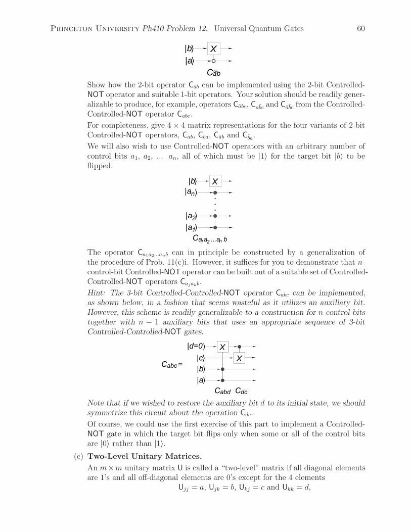
Princeton University Ph410 Problem 12. Universal Quantum Gates 60
Show how the 2-bit operator Cab can be implemented using the 2-bit Controlled-NOT operator and suitable 1-bit operators. Your solution should be readily gener-alizable to produce, for example, operators Cabc, Cabc and Cabc from the Controlled-Controlled-NOT operator Cabc.
For completeness, give 4 × 4 matrix representations for the four variants of 2-bitControlled-NOT operators, Cab, Cba, Cab and Cba.
We will also wish to use Controlled-NOT operators with an arbitrary number ofcontrol bits a1, a2, ... an, all of which must be |1〉 for the target bit |b〉 to beflipped.
The operator Ca1a2...anb can in principle be constructed by a generalization ofthe procedure of Prob. 11(c)i. However, it suffices for you to demonstrate that n-control-bit Controlled-NOT operator can be built out of a suitable set of Controlled-Controlled-NOT operators Cajakb.
Hint: The 3-bit Controlled-Controlled-NOT operator Cabc can be implemented,as shown below, in a fashion that seems wasteful as it utilizes an auxiliary bit.However, this scheme is readily generalizable to a construction for n control bitstogether with n − 1 auxiliary bits that uses an appropriate sequence of 3-bitControlled-Controlled-NOT gates.
Note that if we wished to restore the auxiliary bit d to its initial state, we shouldsymmetrize this circuit about the operation Cdc.
Of course, we could use the first exercise of this part to implement a Controlled-NOT gate in which the target bit flips only when some or all of the control bitsare |0〉 rather than |1〉.
(c) Two-Level Unitary Matrices.
An m×m unitary matrix U is called a “two-level” matrix if all diagonal elementsare 1’s and all off-diagonal elements are 0’s except for the 4 elements
Ujj = a, Ujk = b, Ukj = c and Ukk = d,
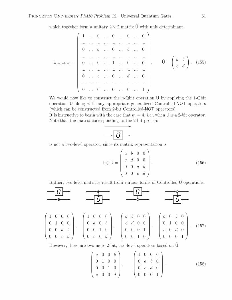
Princeton University Ph410 Problem 12. Universal Quantum Gates 61
which together form a unitary 2 × 2 matrix U with unit determinant,
Utwo−level =
⎛⎜⎜⎜⎜⎜⎜⎜⎜⎜⎜⎜⎜⎜⎜⎜⎜⎜⎜⎜⎜⎜⎝
1 ... 0 ... 0 ... 0 ... 0
... ... ... ... ... ... ... ... ...
0 ... a ... 0 ... b ... 0
... ... ... ... ... ... ... ... ...
0 ... 0 ... 1 ... 0 ... 0
... ... ... ... ... ... ... ... ...
0 ... c ... 0 ... d ... 0
... ... ... ... ... ... ... ... ...
0 ... 0 ... 0 ... 0 ... 1
⎞⎟⎟⎟⎟⎟⎟⎟⎟⎟⎟⎟⎟⎟⎟⎟⎟⎟⎟⎟⎟⎟⎠
, U =
⎛⎝ a b
c d
⎞⎠ . (155)
We would now like to construct the n-Qbit operation U by applying the 1-Qbitoperation U along with any appropriate generalized Controlled-NOT operators(which can be constructed from 2-bit Controlled-NOT operators).
It is instructive to begin with the case that m = 4, i.e., when U is a 2-bit operator.Note that the matrix corresponding to the 2-bit process
is not a two-level operator, since its matrix representation is
I ⊗ U =
⎛⎜⎜⎜⎜⎜⎜⎝
a b 0 0
c d 0 0
0 0 a b
0 0 c d
⎞⎟⎟⎟⎟⎟⎟⎠. (156)
Rather, two-level matrices result from various forms of Controlled-U operations,
⎛⎜⎜⎜⎜⎜⎜⎝
1 0 0 0
0 1 0 0
0 0 a b
0 0 c d
⎞⎟⎟⎟⎟⎟⎟⎠,
⎛⎜⎜⎜⎜⎜⎜⎝
1 0 0 0
0 a 0 b
0 0 1 0
0 c 0 d
⎞⎟⎟⎟⎟⎟⎟⎠,
⎛⎜⎜⎜⎜⎜⎜⎝
a b 0 0
c d 0 0
0 0 0 1
0 0 1 0
⎞⎟⎟⎟⎟⎟⎟⎠,
⎛⎜⎜⎜⎜⎜⎜⎝
a 0 b 0
0 1 0 0
c 0 d 0
0 0 0 1
⎞⎟⎟⎟⎟⎟⎟⎠. (157)
However, there are two more 2-bit, two-level operators based on U,⎛⎜⎜⎜⎜⎜⎜⎝
a 0 0 b
0 1 0 0
0 0 1 0
c 0 0 d
⎞⎟⎟⎟⎟⎟⎟⎠,
⎛⎜⎜⎜⎜⎜⎜⎝
1 0 0 0
0 a b 0
0 c d 0
0 0 0 1
⎞⎟⎟⎟⎟⎟⎟⎠. (158)

Princeton University Ph410 Problem 12. Universal Quantum Gates 62
Deduce transformations of one (or more) of the four basic two-level matrices (157)into the forms (158). Recall that our goal is to perform such transformations usingonly Controlled-NOT operations.
A generalization of this type of procedure to construct higher-dimensional, two-level operators such as that of eq. (155) is described in sec. 4.5.2 of Nielsen andChuang.
(d) Any Unitary Operator is a Product of Two-Level Matrices.
We can show by “brute force” than any n × n unitary matrix U = Ujk can bemultiplied on the left by a sequence of n(n − 1)/2 two-level unitary matrices Ul
such that
Un(n−1)/2 · · ·Ul · · ·U2U1U = I, and so, U = U†1U
†2 · · ·U†
l · · ·U†n(n−1)/2. (159)
The procedure has n − 1 major steps such that after m steps the first m rowsand columns of the product · · ·U2U1U have 1’s on the diagonal and 0’s off thediagonal.
If suffices to show how the first row and column of an m×m unitary matrix canbe transformed via multiplication by m−1 two-level matrices into a matrix L withL1j = Lj1 = 0) except for the first diagonal element which is unity (L11 = 1).
This task is performed using m− 1 two-level matrices of the form
Ul =
⎛⎜⎜⎜⎜⎜⎜⎜⎜⎜⎜⎜⎜⎜⎜⎜⎜⎜⎜⎜⎜⎜⎝
L�11√
|L11|2+|Ll+1,1|20 ... 0
L�l+1,1√
|L11|2+|Ll+1,1|20 ... 0
0 1 ... ... ... ... ... ...
... ... ... ... ... ... ... ...
0 ... ... 1 0 ... ... ...Ll+1,1√
|L11|2+|Ll+1,1|20 ... ... − L11√
|L11|2+|Ll+1,1|20 ... ...
0 ... ... ... 0 1 ... ...
... ... ... ... ... ... ... ...
0 ... ... ... ... ... ... 1
⎞⎟⎟⎟⎟⎟⎟⎟⎟⎟⎟⎟⎟⎟⎟⎟⎟⎟⎟⎟⎟⎟⎠
, (160)
where
L = Ul · · ·U1U =
⎛⎜⎜⎜⎜⎜⎜⎜⎜⎜⎜⎜⎜⎝
L11 L12 ...
0 L22 ...
... ... ...
0 Ll+1,2 ...
Ll+2,1 Ll+2,2 ...
... ... ...
⎞⎟⎟⎟⎟⎟⎟⎟⎟⎟⎟⎟⎟⎠. (161)
That is, each additional multiplication by an appropriate two-level matrix zeroesout one more element in the first column of the product matrix L.
A technicality is that if U1j = 0 for j < l then element L11 is actually zero untilstep l. Since a unitary matrix cannot have all elements of a column equal to zero,sooner or later we obtain L11 = 0.

Princeton University Ph410 Problem 12. Universal Quantum Gates 63
After m − 1 such steps, the product matrix L has all zeroes in its first columnexcept for element L11. Recalling that all rows and columns of a unitary matrixmust be unit vectors, we see that L11 = 1 now. This also implies that all elementsof the first row are zero (except for L11 of course). Thus, after m − 1 steps wehave
L = Um−1 · · ·U1U =
⎛⎜⎜⎜⎜⎜⎜⎝
1 0 ... 0
0 L22 ... L2m
... ... ... ...
0 Lm2 ... Lmm
⎞⎟⎟⎟⎟⎟⎟⎠. (162)
Beginning with the n×n unitary matrix U, we follow the above procedure throughn− 2 major steps (involving a total of (n− 1)+ (n− 2)+ · · ·+2 = n(n− 1)/2− 1steps), at which point the product matrix L is the two-level unitary matrix
L = Un(n−1)/2−1 · · ·U1U =
⎛⎜⎜⎜⎜⎜⎜⎜⎜⎜⎜⎜⎜⎝
1 0 ... ... ... 0
0 1 ... ... ... 0
... ... ... ... ... ...
0 ... ... 1 0 0
0 ... ... 0 Ln−1,n−1 Ln−1,n
0 ... ... 0 Ln,n−1 Lnn
⎞⎟⎟⎟⎟⎟⎟⎟⎟⎟⎟⎟⎟⎠. (163)
Choosing the last two-level matrix to be Un(n−1)/2 = L†, we arrive at eq. (159).
This completes our sketch of the universality for quantum computation of the2-bit Controlled-NOT gate together with the 1-bit gates H and σ1/4
z .
There is no assigned problem in part (d).
Entanglement is Needed for Universality.
It turns out that “almost any” 2-Qbit gate is universal for quantum computation.60
However, the very useful SWAP gate S that was introduced in prob. 6(c) is an exampleof a 2-Qbit gate that is not universal.61 Dodd et al.62 have shown that any 2-Qbit gatethat causes entanglement is universal for quantum computation. Then, Bremner et al.63
have shown that the 2-Qbit gates which are not universal for quantum computationare of only two types, neither of which creates entanglement:
(i) Gates that are direct products of 1-Qbit gates.
(ii) Gates U that are equivalent to the SWAP gate S, meaning that
U = (A ⊗ B)S(C ⊗ D), (164)
where A, B, C and D are 1-Qbit gates.
60 http://physics.princeton.edu/~mcdonald/examples/QM/lloyd_prl_75_346_95.pdfhttp://physics.princeton.edu/~mcdonald/examples/QM/deutsch_prsl_a449_669_95.pdf
61I conjecture that practical quantum computers will involve more SWAP gates than any other kind. ButSWAP gates alone are not sufficient for nontrivial quantum computation.
62 http://physics.princeton.edu/~mcdonald/examples/QM/dodd_pra_65_040301_02.pdf63 http://physics.princeton.edu/~mcdonald/examples/QM/bremner_prl_89_247902_02.pdf

Princeton University Ph410 Problem 12. Universal Quantum Gates 64
Entanglement is not necessary for all types of quantum computation (since by defi-nition any quantum transformation is a computation), but entanglement is requiredfor any approach that has the ambition to encompass all possible types of quantumcomputation (i.e., all possible types of quantum phenomena).64
64Thus, “classic” courses in quantum mechanics that barely mention entanglement exclude the concep-tual bulk of quantum phenomena, typically illustrating only one-particle systems and the small subclass ofmultiparticle interactions involving direct products.

Princeton University Ph410 Problem 13. The Bernstein-Vazirani Problem 65
13. The Bernstein-Vazirani Problem
We now have the vision of a quantum computation as any transformation on a set ofQbits as performed by a unitary operator. In this sense, quantum computation is asolution looking for a problem.
We again take up the quest, begun in prob. 10, for problems that can be solved bya quantum computation in a manner that affords potential advantages compared toclassical computation.
A second example of a quantum computation that is faster than a corresponding classi-cal computation has been given by Bernstein and Vazirani.65 This problem is somewhatartificial, but instructive.
The task is to determine the value of an n-bit integer a by appropriate use of a 1-bitfunction
fa(x) = a · x (mod 2) ≡ a� x. (165)
That is, fa(x) computes the scalar product of a and x when they are regarded asvectors with binary coefficients in an n-dimensional space, and performs the summationmodulo 2.
To determine a via classical computations of fa we would use n applications of it, themth of which sets x = 2m and thereby determines the mth bit of a.
The claim is that a quantum computation can be constructed that determines a in asingle application of fa.
(a) Give a bit-flow diagram for fa(x) as a quantum computation Ufa . The circuitwill have n lines for the n-Qbit input state |x〉n and another line, say |y〉, for the1-Qbit output of f(x). Since the function f depends on the value of the n-bitnumber a, you may find it useful to represent this dependence with an additionaln lines representing the state |a〉n.Hint: Recall prob. 9(c), and note that addition modulo 2 of a set of bits can beimplemented by a succession of bit flips, supposing that the output bit starts as|y〉 = |0〉.The output bit could, of course, begin as a |1〉. Convince yourself that the effectof your circuit can be summarized as
Ufa |a〉|x〉|y〉 = |a〉|x〉|y ⊕ fa(x)〉, (166)
which reminds us of the Deutsch-Jozsa algorithm (prob. 10(f)).
(b) As in the Deutsch-Jozsa algorithm, it is advantageous to perform a quantumcomputation of fa(x) for the n-Qbit state
|x〉n = H⊗n|0〉n =1
2n/2
2n−1∑j=0
|j〉n. (167)
65 http://physics.princeton.edu/~mcdonald/examples/QM/bernstein_siamjc_26_1411_97.pdf
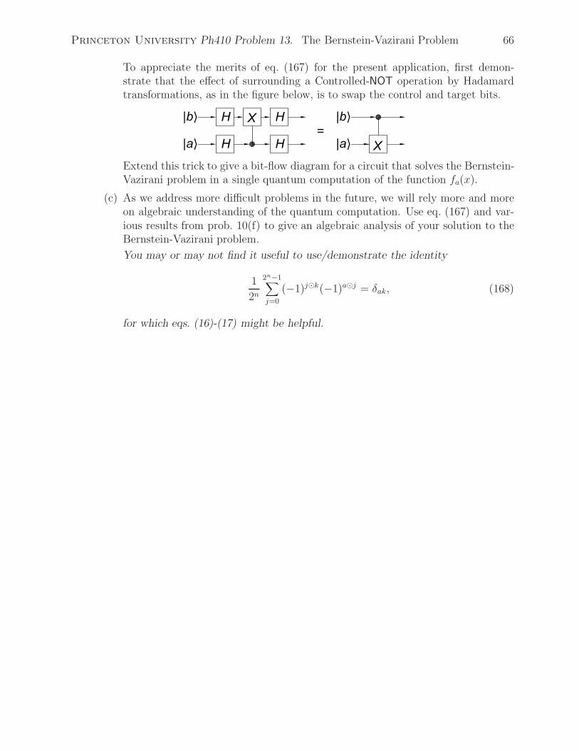
Princeton University Ph410 Problem 13. The Bernstein-Vazirani Problem 66
To appreciate the merits of eq. (167) for the present application, first demon-strate that the effect of surrounding a Controlled-NOT operation by Hadamardtransformations, as in the figure below, is to swap the control and target bits.
Extend this trick to give a bit-flow diagram for a circuit that solves the Bernstein-Vazirani problem in a single quantum computation of the function fa(x).
(c) As we address more difficult problems in the future, we will rely more and moreon algebraic understanding of the quantum computation. Use eq. (167) and var-ious results from prob. 10(f) to give an algebraic analysis of your solution to theBernstein-Vazirani problem.
You may or may not find it useful to use/demonstrate the identity
1
2n
2n−1∑j=0
(−1)j�k(−1)a�j = δak, (168)
for which eqs. (16)-(17) might be helpful.

Princeton University Ph410 Problem 14. Simon’s Problem 67
14. Simon’s Problem
In both problems 10(f) and 13 we have found it advantageous to apply Hadamard gateson all lines of n-Qbit state before and after some operation U is performed.
An additional insight as to why this procedure might be useful is obtained fromeq. (145). Since −1 = eiπ, we can write
H⊗n|j〉n =1
2n/2
2n−1∑k=0
(−1)j�k|k〉n =1
2n/2
2n−1∑k=0
eiπ(j�k)|k〉n. (169)
The second form of eq (169) is reminiscent of a Fourier transform.66 Based on ourexperience with classical Fourier analysis, we anticipate that a quantum version of aFourier transform will be a very powerful computational tool.
A further step towards quantum Fourier analysis was taken by Simon67 who showedthat a quantum algorithm is much faster than a classical one for the determination ofa kind of periodicity of a function.
Suppose we have an n-to-n-bit function fa(x) that is not a one-to-one map, but rathera two-to-one map according to
fa(x) = fa(y) iff y = x⊕ a, (170)
where the binary operation ⊕ as applied to multiple-bit states means bitwise additionmodulo 2. We can say that the function fa is periodic with period a in the restrictedsense of eq. (170).
Simon’s problem is to deduce the value of the “period” a in the minimum number ofapplications of the function f (assuming that the function f is a “black box” with thevalue of a hidden inside).
You may wish to convince yourself (without it being part of the written assignment)that y = x⊕ a implies that x⊕ y = a, and that x⊕ a · · · ⊕ a is either x or y dependingon whether there are an even or odd number of additions.
66Indeed, this operation was called a discrete quantum Fourier transform inhttp://physics.princeton.edu/~mcdonald/examples/QM/bernstein_siamjc_26_1411_97.pdfbut we now reserve that name for the operation studied in prob. 17.
67 http://physics.princeton.edu/~mcdonald/examples/QM/simon_siamjc_26_1474_97.pdf

Princeton University Ph410 Problem 14. Simon’s Problem 68
(a) Approximately how many evaluations of the classical n-bit function fa would berequired to deduce the value of the n-bit number a?
(b) Turning to a quantum computation involving Simon’s n-bit function fa(x), wenote that this function cannot be represented by a unitary transformation, since itis a two-to-one function. However, we can extend the trick of Deutsch’s algorithmto embed fa inside a unitary transformation Ufa on 2n Qbits according to
Ufa |x〉n|y〉n = |x〉n|y ⊕ fa(x)〉n, (171)
where |x〉n and |y〉n are each n-Qbit states.
You can readily convince yourself that Ufa of eq. (171) is a reversible operation,and hence unitary.
Extrapolating from our experience with Deutsch’s algorithm and the Bernstein-Vazirani problem, we anticipate that it will be useful to begin with states |x〉nand |y〉n as |0〉n, and apply Hadamard transformations before and after operationUfa to all of the x and/or the y lines.
Explore the choice of applying the Hadamard transformations only to the x lines.
Note that
Ufa
2n−1∑j=0
|j〉n|0〉n =2n−1∑j=0
|j〉n|f(j)〉n, (172)
and since fa is a two-to-one function such that fa(x) = fa(x ⊕ a), we can alsowrite eq. (172) as
Ufa
2n−1∑j=0
|j〉n|0〉n =1√2
2n−1∑j=0
(|j〉n + |j ⊕ a〉n)|fa(j)〉n. (173)
Analyze the transformation
H⊗nx UfaH
⊗nx |0〉x|0〉y (174)
to deduce a procedure to determine the value of a, based on repetitions of thisoperation, each ending with a measurement of the output state. That is, Si-mon’s problem is solved by a probabilistic quantum computation, in contrast tothe Deutsch-Jozsa problem and the Bernstein-Vazirana problem which can besolved by deterministic computation.
You should find that it would take only of order n repetitions, and hence thequantum solution to Simon’s problem is exponentially faster than the classicalsolution. This result suggests that there can be spectacular advantages of quan-tum computation over classical computation for some types of problems.
The premise of this problem is that the function fa has a period in the sense ofeq. (170). A related problem would be to show whether or not a given n-to-n-bitfunction has such a period.

Princeton University Ph410 Problem 15. Grover’s Search Algorithm 69
15. Grover’s Search Algorithm
While Simon’s problem shows that a quantum computation can be exponentially fasterthan its classical counterpart, one would probably not be willing to pay money to solvethat particular problem. An example of a computational problem that is significantenough to attract funding, and for which a quantum solution is faster than a classicalone, is the task of searching a list (a database) for a particular entry whose location isnot known.68
We will cast this problem into the form of a “randomized” list of n-bit integers (aphone book?) in which we need to locate the integer a. We suppose that we have afunction fa that can recognize the desired integer according to
fa(x) =
⎧⎪⎨⎪⎩
0, x = a,
1, x = a.(175)
To locate the number a in our randomized list with certainty via classical computationusing function fa, we need to examine every entry in the list, i.e., we must make 2n
evaluations of fa.69 If we make m < n classical evaluations, the probability of success
is, of course, only P = m/n.
(a) It should be no surprise by now that a quantum search for the number a will beassisted by the unitary function Ufa defined by
Ufa |x〉n|y〉 = |x〉n|y ⊕ fa(x)〉, (176)
where |x〉n is an n-Qbit state and |y〉 is a single Qbit.
Give a bit-flow diagram of a possible implementation of the operation Ufa . Thecircuit should include n lines for |a〉, so that it could be “programmed” to searchfor different values of a. That is, expand eq. (176) to
Ufa |a〉n|x〉n|y〉 = |a〉n|x〉n|y ⊕ fa(x)〉. (177)
A circuit for this exists that uses no ancillary lines.
(b) To search through all values of x as quickly as possible, we will certainly want touse the trick of eq. (130),
|φ〉n = H⊗n|0〉n =1
2n/2
2n−1∑j=0
|j〉n, (130)
by initializing |x〉 to |0〉n and applying Hadamard transformations to all of theinput lines.
68 http://physics.princeton.edu/~mcdonald/examples/QM/grover_prl_79_325_97.pdfhttp://physics.princeton.edu/~mcdonald/examples/QM/grover_prl_79_4709_97.pdfhttp://physics.princeton.edu/~mcdonald/examples/QM/grover_prl_80_4329_98.pdf
69 More precisely, we need 2n − 1 classical evaluations of f to locate a with certainty, since if we haveexamined all but one of the entries in the list and not found a, we are certain that the remaining entry is a,provided we have the additional knowledge that the list is complete and without duplications.

Princeton University Ph410 Problem 15. Grover’s Search Algorithm 70
Recall Deutsch’s algorithm (Prob. 10) to show that an appropriate initializationof the auxiliary bit |y〉 leads to no change in |y〉 but to a “marking” of the desiredstate |j = a〉n after Ufa is applied to the direct product state |φ〉n|y〉.This kind of marking is a nonclassical effect that arises because the amplitude ofa direct-product quantum state is a shared property of all of the components ofthat state. Of course, we cannot determine the details of an unknown quantumstate in a small number of operations, so we must still find a way to exploit the“marking” in an efficient manner.
You should find that the “marking” consists of changing the sign of the amplitudeof the state |a〉n in eq. (130), leaving all other |j〉n unchanged. A useful way tothink about the “marking” process is that when |y〉 is properly prepared, the effectof Ufa on |x〉n is a reflection in a 2n-dimensional space about the (hyper)planeperpendicular to the desired state |a〉n. That is, if we write
|φ〉n =1
2n/2|a〉n + β|b〉n, (178)
where |b〉n is orthogonal to |a〉n, then
Ufa |φ〉n|y〉 =[− 1
2n/2|a〉n + β|b〉n
]|y〉. (179)
If we observe either of the states |φ〉n or Ufa |φ〉n,70 the probability that we findit to be the desired state |a〉n is only 1/2n, so we have not immediately found agood search algorithm.
A geometric view of what we have accomplished is also very helpful.71 The desiredstate |a〉n is nearly orthogonal to the state |φ〉n, since
〈a|φ〉n =1
2n/2= cos(π/2 − θ) = sin θ, (180)
where the angle θ is a measure of the separation between the state |φ〉n and thestate |b〉n that is orthogonal to |a〉n, as shown in the figure. The state Ufa |φ〉n isthe reflection of state |φ〉n about the |b〉n axis.
70We suppress mention of the auxiliary bit |y〉 in much of the remainder of this problem.71 The geometric view given here of Grover’s algorithm first appeared in the useful review
http://physics.princeton.edu/~mcdonald/examples/QM/aharonov_quant-ph-9812037.pdfbased on an algebraic argument given inhttp://physics.princeton.edu/~mcdonald/examples/QM/boyer_fphys_46_493_98.pdf

Princeton University Ph410 Problem 15. Grover’s Search Algorithm 71
(c) Grover realized that further reflections in the state-space of |x〉n provide a meansof strengthening the “marking” of the desired state |a〉n, such that after 2n/2
reflections a measurement of the evolved state of |x〉n will result in state |a〉n withhigh probability.
Indeed, we see from the figure that if we reflect the state Ufa |φ〉n about the |φ〉naxis, using the operation U|φ〉n, the final state has been rotated by angle 2θ towardsthe |a〉n axis.
If we iterate this pair of reflections about the |b〉n and |φ〉n axes m times, thenthe state |φ〉n will have been rotated to angle (2m + 1)θ with respect to the |b〉naxis. If the final angle is close to π/2, then a measurement of the state will yield|a〉n with high probability, as desired. Thus, we need
(2m+ 1)θ ≈ 2m+ 1
2n/2≈ π
2≈ 2, (181)
That is, with m = 2n/2 =√N iterations of the transformation U|φ〉nUfa , where
N = 2n is the size of the list, a measurement of the state (U|φ〉nUfa)m|φ〉n is almost
certain to be |a〉n. The probability of failure is approximately 1/2n, so if we failto find the state |a〉n at the end of the first set of iterations, we repeat the entireprocedure. The probability of failing twice is 1/22n, etc. Thus, Grover’s searchalgorithm reduces the task of finding an item in a randomized list of length Nfrom ≈ N classical samplings of the list to only ≈ √
N quantum samplings.
Grover’s procedure does not converge for the case that n = 1, i.e., when the listcontains only 2 items. But then, we can find an item classically with only a singlelook into the list. However, for n = 2, i.e., a list of 4 items, sin θ = 1/
√22 = 1/2
so θ = 30◦. We see from the figure on the previous page that a single iterationbrings the state |φ〉2 exactly onto |a〉2. Grover’s quantum search finds 1 item in alist of 4 in a single “enquiry”.
It remains to construct the reflection U|φ〉n, based on the state |φ〉n, which has theeffect on a general state
|ψ〉n =N−1∑j=0
ψj|j〉n, (182)
where N = 2n, of reflecting it about the |φ〉n “axis”. Decompose the state (182)into its component “along” state |φ〉n and the remainder (which is thereby or-thogonal to |φ〉n), introducing the notation
⟨ψj⟩
=1
N
N−1∑j=0
ψj =1√N〈φ|ψ〉n. (183)
Then, consider the form of Uφ|ψ〉n to express U|φ〉n as a kind of projection operatorinvolving the state |φ〉n. Show that the effect of reflecting |ψ〉n about |φ〉n is to
change the sign of each amplitude ψj−⟨ψj⟩, which was called a “reflection about
the mean” by Grover.
Sketch the steps of the appropriate set of iterations for the case that n = 3,starting with the state |φ〉3 represented as a “comb” of 8 basis states of equal

Princeton University Ph410 Problem 15. Grover’s Search Algorithm 72
amplitude, as shown below. What is the probability of success of Grover’s searchalgorithm in this case?
Show also that the transformation Ufa can be expressed via a projection operatorinvolving state |a〉n.
(d) While we have expressed the transformation U|φ〉n as a projection operator, thisdoes not immediately tell us how we could construct this operator out of elemen-tary quantum gates.
Since operator U|φ〉n is a reflection about |φ〉n and
|φ〉n = H⊗n|0〉n, (130)
we can relate the reflection about |φ〉n to the reflection U|0〉n about |0〉n accordingto
U|φ〉n = H⊗nU|0〉nH⊗n. (184)
Equation (184) may be more self evident using the representation of U|φ〉n in termsof the projection operator that you have deduced in part (c).
Further, Grover’s search algorithm is unaffected if the amplitudes of all states aremultiplied by −1. That is, the operator −U|φ〉n could be used instead of U|φ〉n.Since the reflection U|φ〉n changes the sign of the amplitude of any state thatis orthogonal to |φ〉n while leaving the amplitude of the state |φ〉n unchanged,operator −U|φ〉n changes the sign of the amplitude of the state |φ〉n but does notchange the amplitude of any state that is orthogonal to |φ〉n. Thus, −U|φ〉n is areflection about the plane perpendicular to state |φ〉n.Combining this insight with eq. (184), we see that we need the operator thatdescribes a reflection about the plane perpendicular to the state |0〉n. Recallingthat the operator Ufa of part (a) is the reflection about the plane perpendicular tothe state |a〉n (Ufa = −U|a〉n), we see that using operator Uf0 in eq. (184) providesus with the desired construction of U|φ〉n.
Simplify your construction of Ufa for the particular case that |a〉n = |0〉n. Summa-rize briefly how the m iterations of Grover’s search algorithm can be built up froman appropriate initial state, followed by a minimal set of products of operators.

Princeton University Ph410 Problem 16. Parity of a Function 73
16. Parity of a Function
At this point we might be optimistic that all classical computations could be performedsignificantly faster by an appropriate quantum computation. However, this appearsnot to be so,72 as we will illustrate in this problem.
Consider an n-bit to 1-bit function f(x), i.e., f(x) = 0 or 1. The parity Πf of functionf is defined as73
Πf =2n−1∏j=0
(−1)f(j) = (−1)∑2n−1
j=0f(j)
. (185)
A classical computation of Πf requires 2n evaluations of the n-bit function f .
For a quantum computation of Πf it seems appropriate to introduce the unitary func-tion Uf defined by
Uf |x〉n|y〉 = |x〉n|y ⊕ f(x)〉, ) (186)
that we first encountered in the Deutsch-Jozsa algorithm (prob. 10(f)).
Show that use of the above circuit permits a determination of the parity of f in a singleuse of Uf for the case that n = 1. This is a good start, since 2 evaluations of f areneeded for a classical computation of Πf when n = 1.
Hint: Note that (−1)f = (−1)−f when f = 0 or 1 only. Thus,
(−1)f(1) = (−1)f(0)(−1)f(1)−f(0) = (−1)f(0)(−1)f(1)+f(0) = (−1)f(0)Πf . (187)
The example of n = 1 affords a glimpse that an application of Uf can be used togroup the phase factors (−1)f(x) into pairs. To build up Πf in this manner, the phase(−1)f(0) can be grouped together with the phases (−1)f(1).....(−1)f(2n−1−1) during 2n−1
applications of Uf (together with a shift operator Sn) into the amplitude of the first
72 http://physics.princeton.edu/~mcdonald/examples/QM/farhi_prl_81_5442_98.pdfhttp://physics.princeton.edu/~mcdonald/examples/QM/beals_quant-ph-9802049.pdf
73 Note that there are two technical meanings to the term parity. The computational definition, usedin this problem, relates to whether a bit string contains an even or odd numbers of 1’s. The quantummechanical definition (due to Wigner) relates to the sign of the eigenvalue of the transformation of spaceinversion (r → −r) that was mentioned in prob. 4(e).

Princeton University Ph410 Problem 16. Parity of a Function 74
2n−1 basis states, while at the same time the product of the second 2n−1 phase factorsbecomes the amplitude of the second 2n−1 basis states:
|0〉n → |ψ〉n =1
2n/2
2n−1−1∏k=0
(−1)f(k)2n−1−1∑j=0
|j〉n +1
2n/2
2n−1∏k=2n−1
(−1)f(k)2n−1∑j=2n−1
|j〉n. (188)
We see that if Πf = 1, then
|ψ〉n =1
2n/2
2n−1∑j=0
|j〉n = H⊗n|0〉n = |φ〉n, (Πf = 1), (189)
recalling eq. (130), so that a final Hadamard transformation will return this state to|0〉n,
H⊗n|ψ〉n = |0〉n, (Πf = 1). (190)
On the other hand, if Πf = −1, then |ψn〉 is orthogonal to |φ〉n, and the final Hadamardtransformation will bring it to some state orthogonal to |0〉n. Thus, a measurement ofthe final state reveals the parity of function f with certainty (Πf = 1 if the final stateis observed to be |0〉n, and Πf = 1 otherwise), but only after 2n−1 evaluations of thefunction f .
For details, and a demonstration that Πf cannot be determined in less than 2n−1
evaluations of f , see the references in the footnote on the previous page, sec. 6.7 ofPreskill’s lectures, or sec. 6.7 of Nielsen and Chuang.
For the record, the needed shift operator Sn (which is a generalization of the two-bitSWAP operator Sab of prob. 6(c)) obeys
Sn|j〉n =
⎧⎪⎪⎪⎪⎪⎪⎪⎪⎨⎪⎪⎪⎪⎪⎪⎪⎪⎩
|j + 1〉n, j = 0, ..., 2n−1 − 2,
|0〉n, j = 2n−1 − 1,
|j + 1〉n, j = 2n−1, ...., 2n− 2,
|2n−1〉n, j = 2n − 1,
(191)
and the full algorithm can be summarized as
(H⊗nx ⊗ XyHy)(UfSn)
2n−1−1Uf (H⊗nx ⊗HyXy)|0〉x|0〉y =
1 + Πf
2|0〉n|0〉y +
1 − Πf
2|a〉n|0〉y,
(192)where |a〉n is a normalized state orthogonal to |0〉n.
Bottom line: There are some computations for which quantum algorithms provide noadvantage classical ones.74
74 This negative conclusion makes the success of Grover’s search algorithm (for a list of 2n entries) allthe more impressive. Part of that success lies in the fact that Grover’s algorithm is only (highly) probablysuccessful after its m ≈ 2n/2 iterations. A guarantee of success, however, cannot be given unless there are atleast 2n−1 evaluations of the function f(x), which is essentially the same guarantee as available in a classicalcomputation.
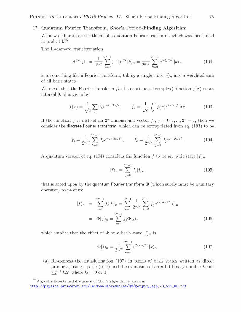
Princeton University Ph410 Problem 17. Shor’s Period-Finding Algorithm 75
17. Quantum Fourier Transform, Shor’s Period-Finding Algorithm
We now elaborate on the theme of a quantum Fourier transform, which was mentionedin prob. 14.75
The Hadamard transformation
H⊗n|j〉n =1
2n/2
2n−1∑k=0
(−1)j�k|k〉n =1
2n/2
2n−1∑k=0
eiπ(j�k)|k〉n. (169)
acts something like a Fourier transform, taking a single state |j〉n into a weighted sumof all basis states.
We recall that the Fourier transform fk of a continuous (complex) function f(x) on aninterval [0,a] is given by
f(x) =1√a
∑k
fke−2πikx/a, fk =
1√a
∫ a
0f(x)e2πikx/adx. (193)
If the function f is instead an 2n-dimensional vector fj, j = 0, 1, ..., 2n − 1, then weconsider the discrete Fourier transform, which can be extrapolated from eq. (193) to be
fj =1
2n/2
2n−1∑k=0
fke−2πijk/2n
, fk =1
2n/2
2n−1∑j=0
fje2πijk/2n
. (194)
A quantum version of eq. (194) considers the function f to be an n-bit state |f〉n,
|f〉n =2n−1∑j=0
fj|j〉n, (195)
that is acted upon by the quantum Fourier transform Φ (which surely must be a unitaryoperator) to produce
|f〉n =2n−1∑k=0
fk|k〉n =2n−1∑k=0
1
2n/2
2n−1∑j=0
fje2πijk/2n|k〉n
= Φ|f〉n =2n−1∑j=0
fjΦ|j〉n (196)
which implies that the effect of Φ on a basis state |j〉n is
Φ|j〉n =1
2n/2
2n−1∑k=0
e2πijk/2n|k〉n. (197)
(a) Re-express the transformation (197) in terms of basis states written as directproducts, using eqs. (16)-(17) and the expansion of an n-bit binary number k and∑n−1
0 kl2l where kl = 0 or 1.
75A good self-contained discussion of Shor’s algorithm is given inhttp://physics.princeton.edu/~mcdonald/examples/QM/gerjuoy_ajp_73_521_05.pdf

Princeton University Ph410 Problem 17. Shor’s Period-Finding Algorithm 76
(b) Transcribe the result of part (a) into a bit-flow diagram. The input lines can be“overwritten” to become the output lines.
Hint: Your result from part (a) should show a simple relation between the highest-order bit of the output state and the lowest-order bit of the input state. It sufficesto “read” the output lines in reverse order to the input lines, eliminating a tediousn-bit SWAP operation.76 Recall eq. (61), and use a small variation on the spiritof prob. (12) to express any needed 1-bit gates as powers of H and Z = (σ1/4
z )4.
(c) Give a bit-flow diagram for the operation Φ−1 that performs the inverse Fouriertransform,
Φ−1|f〉n = |f〉n. (198)
(d) Shor’s Period-Finding Algorithm.77
While the quantum Fourier transform requires fewer gates than the classical dis-crete Fourier transform, and so is faster in a sense, its output is a quantumstate whose value cannot be well determined in a small number of repetitions.The quantum Fourier transform will never be an all-purpose replacement for theclassical discrete Fourier transform. We are left with the task of finding specialproblems of interest for which the quantum Fourier transform is a better solutionthan the classical Fourier transform.
As a first example, consider the problem of finding the period a of an n-to-n-bitfunction f(x) that obeys
f(y) = f(x), if y = x+ma, (199)
where a and m are integers (< 2n−2). Unlike, say, a violin, the function f has onlya single period. The simplicity of this function may permit a quantum analysisto be advantageous.
This problem is similar to Simon’s problem (prob. 14), except that now the con-dition of periodicity involves ordinary addition, which is more complicated thanaddition modulo 2.
As in Simon’s problem, consider the unitary operator Uf that links two n-bitstates |x〉n and |y〉n together with the function f(x) according to
Uf |x〉n|y〉n = |x〉n|y ⊕ f(x)〉n. (171)
And also as in Simon’s problem, we begin by applying Hadamard transformationsto the x lines to produce the state
UfH⊗nx |0〉x|0〉y =
1
2n/2
2n−1∑j=0
|j〉x|f(j)〉y. (200)
Because function f is periodic with period a, there are only a distinct states of|f(j)〉y. Therefore, the sum in eq. (200) can be rearranged into a groups each
76In the following problem we consider an alternative algorithm that builds in the SWAP operation suchthat all two-Qbit gates involve neighboring lines.
77 http://physics.princeton.edu/~mcdonald/examples/QM/shor_ieeefcs_35_124_94.pdfhttp://physics.princeton.edu/~mcdonald/examples/QM/shor_siamjc_26_1484_97.pdf
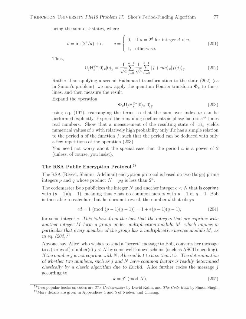
Princeton University Ph410 Problem 17. Shor’s Period-Finding Algorithm 77
being the sum of b states, where
b = int(2n/a) + c, c =
⎧⎪⎨⎪⎩
0, if a = 2d for integer d < n,
1, otherwise.(201)
Thus,
UfH⊗nx |0〉x|0〉y =
1√a
a−1∑j=0
1√b
b−1∑m=0
|j +ma〉x|f(j)〉y . (202)
Rather than applying a second Hadamard transformation to the state (202) (asin Simon’s problem), we now apply the quantum Fourier transform Φx to the xlines, and then measure the result.
Expand the operationΦxUfH
⊗nx |0〉x|0〉y (203)
using eq. (197), rearranging the terms so that the sum over index m can beperformed explicitly. Express the remaining coefficients as phase factors eiφ timesreal numbers. Show that a measurement of the resulting state of |x〉n yieldsnumerical values of x with relatively high probability only if x has a simple relationto the period a of the function f , such that the period can be deduced with onlya few repetitions of the operation (203).
You need not worry about the special case that the period a is a power of 2(unless, of course, you insist).
The RSA Public Encryption Protocol.78
The RSA (Rivest, Shamir, Adelman) encryption protocol is based on two (large) primeintegers p and q whose product N = pq is less than 2n.
The codemaster Bob publicizes the integer N and another integer c < N that is coprimewith (p− 1)(q − 1), meaning that c has no common factors with p− 1 or q − 1. Bobis then able to calculate, but he does not reveal, the number d that obeys
cd = 1 (mod (p− 1)(q − 1)) = 1 + e(p− 1)(q − 1), (204)
for some integer e. This follows from the fact that the integers that are coprime withanother integer M form a group under multiplication modulo M , which implies inparticular that every member of the group has a multiplicative inverse modulo M , asin eq. (204).79
Anyone, say, Alice, who wishes to send a “secret” message to Bob, converts her messageto a (series of) number(s) j < N by some well-known scheme (such as ASCII encoding).If the number j is not coprime withN , Alice adds 1 to it so that it is. The determinationof whether two numbers, such as j and N have common factors is readily determinedclassically by a classic algorithm due to Euclid. Alice further codes the message jaccording to
k = jc (mod N), (205)
78Two popular books on codes are The Codebreakers by David Kahn, and The Code Book by Simon Singh.79More details are given in Appendices 4 and 5 of Nielsen and Chuang.
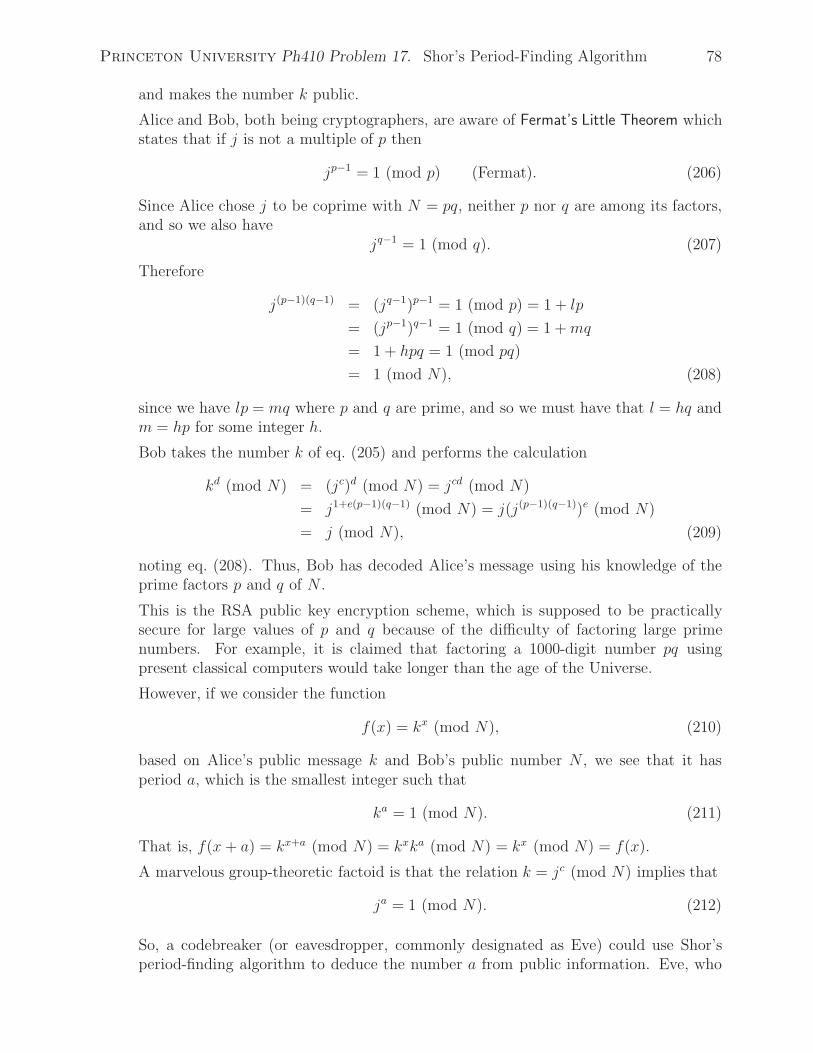
Princeton University Ph410 Problem 17. Shor’s Period-Finding Algorithm 78
and makes the number k public.
Alice and Bob, both being cryptographers, are aware of Fermat’s Little Theorem whichstates that if j is not a multiple of p then
jp−1 = 1 (mod p) (Fermat). (206)
Since Alice chose j to be coprime with N = pq, neither p nor q are among its factors,and so we also have
jq−1 = 1 (mod q). (207)
Therefore
j(p−1)(q−1) = (jq−1)p−1 = 1 (mod p) = 1 + lp
= (jp−1)q−1 = 1 (mod q) = 1 +mq
= 1 + hpq = 1 (mod pq)
= 1 (mod N), (208)
since we have lp = mq where p and q are prime, and so we must have that l = hq andm = hp for some integer h.
Bob takes the number k of eq. (205) and performs the calculation
kd (mod N) = (jc)d (mod N) = jcd (mod N)
= j1+e(p−1)(q−1) (mod N) = j(j(p−1)(q−1))e (mod N)
= j (mod N), (209)
noting eq. (208). Thus, Bob has decoded Alice’s message using his knowledge of theprime factors p and q of N .
This is the RSA public key encryption scheme, which is supposed to be practicallysecure for large values of p and q because of the difficulty of factoring large primenumbers. For example, it is claimed that factoring a 1000-digit number pq usingpresent classical computers would take longer than the age of the Universe.
However, if we consider the function
f(x) = kx (mod N), (210)
based on Alice’s public message k and Bob’s public number N , we see that it hasperiod a, which is the smallest integer such that
ka = 1 (mod N). (211)
That is, f(x+ a) = kx+a (mod N) = kxka (mod N) = kx (mod N) = f(x).
A marvelous group-theoretic factoid is that the relation k = jc (mod N) implies that
ja = 1 (mod N). (212)
So, a codebreaker (or eavesdropper, commonly designated as Eve) could use Shor’speriod-finding algorithm to deduce the number a from public information. Eve, who

Princeton University Ph410 Problem 17. Shor’s Period-Finding Algorithm 79
also knows Bob’s public number c, can now use a classical computer to calculate thenumber d′ that obeys
cd′ = 1 (mod a) = 1 + ga, (213)
for some integer g. She then calculates
kd′(mod N) = (jc)d
′(mod N) = jcd
′(mod N)
= j1+ga (mod N) = j(ja)g (mod N)
= j (mod N), (214)
noting eq. (212). Thus, Eve, with her quantum computer, has broken the supposedlyunbreakable RSA encryption scheme.
Of course, Eve’s quantum computer needs twice as many bits as there are in the numberN . If N has 1000 decimal digits, it has 3322 binary digits, so the quantum computerneed 6644 Qbits. The largest quantum computer to date has 7 Qbits.
Furthermore, the quantum Fourier transform requires two-bit gates that couple Qbitsthat are far removed from one another.
A “natural” homework assignment would be to construct the operation Uf now thatwe know what the relevant function f is. However, this exercise turns out to beconsiderably more involved that the construction of Φ = UFT, and we defer it to thefollowing problem.
Factoring
Shor’s algorithm is often described as providing a fast way to factor large numbers.But so far we have avoided the explicit task of factoring Bob’s number N , even thoughwe have succeeded in breaking the RSA code based on it. Here we give a very briefsketch of how Alice (or Eve) might factor Bob’s number N = pq.80
Alice again starts with a number j that is coprime with N , but now she simply choosesthis at random. With her quantum computer she deduces the period a of the functionf(x) = jx mod N . As in eq. (211), the period a is the smallest integer such that
ja = 1 (mod N). (215)
If a turns out to be odd, she tries another j until the corresponding a is found to beeven. She then checks the value of ja/2 (mod N), and iterates until this value is not−1, i.e., not N − 1. The claim is that the probability of choosing a “good” value of jon the first try is greater than 50%.
The meaning of “good” is illustrated by the fact that the following identity is nownontrivial,
0 = ja − 1 (mod N) = (ja/2 − 1)(ja/2 + 1) (mod N). (216)
Since a is the smallest number such that eq. (215) holds, neither ja/2 − 1 nor ja/2 + 1is a multiple of N , but their product is. As N = pq where p and q are prime, it mustbe that p is a factor of ja/2 − 1 and q is a factor of ja/2 + 1, or vice versa. Then, p (or
80Greater detail is given in sec. 5.3 of Nielsen and Chuang, and in Appendix 3 to Mermin’s Lecture 3.

Princeton University Ph410 Problem 17. Shor’s Period-Finding Algorithm 80
q) is the greatest common divisor of N and ja/2 − 1, as can be extracted efficiently bya classical algorithm due to Euclid.
Accuracy of the Quantum Fourier Transform
The quantum Fourier transform Φ|f〉n of an n-Qbit function f , where |f〉n =∑2n−1j=0 fj|j〉n,
is
Φ|f〉n =2n−1∑k=0
1
2n/2
2n−1∑j=0
fje2πijk/2n|k〉n =
2n−1∑k=0
1
2n/2
2n−1∑j=0
fjeiφjk |k〉n, (196)
which involves 22n phases φjk = 2πjk/2n most of which are extremely tiny. In practice
it will be impossible to construct accurately the quantum phase gates Z1/2mfor m of
order n as needed to implement these phase factors in the quantum Fourier transform(according to your solution to part (b).).
However, as discussed in part (d), Shor’s use of the quantum Fourier transform is onlyto find the period of a function with high probability. In particular, if the function fhas a period a, the probability of observing a state |k〉n is large (and of order 1/a) onlyfor a set of a of these states. So, the practical question is to what extent “errors” inthe phase factors of eq. (197) alter the probability
P (k) =1
2n
∣∣∣∣∣∣2n−1∑j=0
fjeiφjk
∣∣∣∣∣∣2
, (217)
that a state |k〉n would be observed during the measurement of the Fourier transformedstate (196) at the end of the period-finding algorithm.
Suppose that each of the phases φjk is altered by a small amount δjk, and δ is the
maximum of the |δjk| Then, eiφjk → ei(φjk+δjk) ≈ eiφjk(1 + iδjk), and
P (k) → 1
2n
∣∣∣∣∣∣2n−1∑j=0
fjei(φjk+δjk)
∣∣∣∣∣∣2
≈ 1
2n
∣∣∣∣∣∣2n−1∑j=0
fjeiφjk(1 + iδjk)
∣∣∣∣∣∣2
≈ P (k) +2
2nIm
⎡⎣2n−1∑j=0
δjkf�j e
−iφjk
2n−1∑j′=0
fj′eiφj′k
⎤⎦ . (218)
Now,
2
2n
∣∣∣∣∣∣Im⎡⎣2n−1∑j=0
δjkf�j e
−iφjk
2n−1∑j′=0
fj′eiφj′k
⎤⎦∣∣∣∣∣∣ ≤ 2
2n
∣∣∣∣∣∣2n−1∑j=0
δjkf�j e
−iφjk
2n−1∑j′=0
fj′eiφj′k
∣∣∣∣∣∣≤ 2δ
2n
∣∣∣∣∣∣2n−1∑j=0
fjeiφjk
∣∣∣∣∣∣2
= 2δP (k), (219)
so the effect of the “errors” δjk is to multiply the relevant probabilities by a factorbounded by 1 ± 2δ.
A corollary is that it is not necessary to implement the (controlled) phase gates Z1/2m
for m > 10 if we are content with the probabilities of the period-finding algorithm tobe accurate to 1%.81
81This was first discussed by D. Coppersmith,http://physics.princeton.edu/~mcdonald/examples/QM/coppersmith_ibm_rc19642_94.pdf

Princeton University Ph410 Problem 18. Nearest-Neighbor Algorithms 81
18. Nearest-Neighbor Algorithms
The interest in codebreaking is so great that substantial effort has gone into explorationof variations on Shor’s period-finding algorithm and into its potential implementationvia quantum gates. In this course we do not have time to review such related themesas discrete logarithms, hidden subgroups, order-finding, and phase estimation, whichare treated in Nielsen and Chuang.
Turning to the issue of implementation of Shor’s algorithm, there are two broad choices:
A. “Fast” algorithm’s that involve a minimal number of steps in the computation,i.e., smaller depth of the quantum circuit, typically at the expense of requiringlarger numbers of Qbits.82
B. Low-Qbit-count algorithms, which typically require greater circuit depth.83
An additional issue is that the “standard” algorithms that we have explored for n-bitproblems all require two-bit gates that relate “distant” Qbits.
While the optical Controlled-NOT gates studied in prob. 7(e) might indeed work equallywell for any pair of Qbits, this is not the case for a large class of proposed quantumcomputers in which Qbits are encoded on the spins of electrons, atoms or molecules.In the spin-based systems, interactions between Qbits are due to their magnetic dipolecouplings, whose strength falls off with distance as 1/r3. If these systems are to serveas viable quantum computers, the computations they perform should involve onlynearest-neighbor gates.
In general, a two-bit operation Uj,j+k involving bits j and j + k that are members of alinearly ordered set could be performed by a sequence of k− 1 nearest-neighbor SWAPoperations, Sm,m+1 (prob. 6(c)),
followed by the nearest-neighbor operation Uj,j+1,
Uj,j+k = Sj+k−1,j+kSj+k−2,j+k−1 · · · Sj+1,j+2Uj,j+1. (220)
The swapping of locations of the bits might increase the distance between pairs of bitsused in later two-bit operators, requiring ever larger numbers of SWAP operations iffurther operations are to involve only neighboring bits. Fortunately, this is not thecase for circuits that implement Shor’s algorithm.
82 http://physics.princeton.edu/~mcdonald/examples/QM/zalka_quant-ph-9806084.pdfhttp://physics.princeton.edu/~mcdonald/examples/QM/gossett_quant-ph-9808061.pdfhttp://physics.princeton.edu/~mcdonald/examples/QM/cleve_quant-ph-0006004.pdf
83 http://physics.princeton.edu/~mcdonald/examples/QM/beauregard_quant-ph-0205095.pdfhttp://physics.princeton.edu/~mcdonald/examples/QM/fowler_qic_4_237_04.pdf

Princeton University Ph410 Problem 18. Nearest-Neighbor Algorithms 82
(a) Fourier Transform.
Give a bit-flow diagram of a circuit for the quantum Fourier transform Φ (prob. 17(b))that involves only nearest-neighbor gates. By associating one nearest-neighborSWAP operation with each of the needed Controlled-Zp gates, you should be ableto implement the latter as nearest-neighbor gates also. And, you should be ableto arrange the swaps so that the order of the output lines is reversed, bringingthem into alignment with the input lines.
Begin by giving a diagram for the case of 3 Qbits, and verify that your circuitworks well for 4 Qbits.
Your diagram should show groups of gates on adjacent pairs of lines. It will bepossible in some hardware realizations of the circuit to coalesce each of these logi-cal groups into a single physical two-Qbit gate, so the nearest-neighbor algorithmwill not have excessive depth.
(b) Fourier Addition.
In prob. 9(g) we considered a quantum circuit that adds two numbers a and b.Some (slight) complexity of that circuit was needed to deal with “carrying” whenadding bits that are both |1〉. Expand the quantum Fourier transform Φ|a + b〉nin a manner similar to that for Φ|j〉n in prob. 17(a) and draw a nearest-neighborcircuit that we will call Φ+
a (b), which uses |a〉n and Φ|b〉n as its inputs, overwritingthe latter to become Φ|a+ b〉n without any “carry” operations. Note that in thisprocedure, numbers a and b must have only n− 1 bits, while their sum a+ b mayhave n bits.
Thus, at the expense of performing quantum Fourier transforms and their inverse,we obtain an adder circuit that uses 2n + 2 bits to add two n-bit numbers, incontrast to the use of 3n + 1 bits in the circuit of prob. 9(g).
It suffices to give a circuit for the case that a and b are 3-bit numbers. Of course,the sum then has 4 bits. Before deducing a nearest-neighbor version of the circuit,it may be useful to give a non-nearest-neighbor circuit modeled after your solutionto prob. 17(a).
(c) Fourier Subtraction.
By Φ−a (b) we mean the operation that uses |a〉n and Φ|b〉n as inputs, where a
and b are (n − 1)-bit numbers, and applies the inverse of the gates of operationΦ+a (b) in reverse order. Using your expansion for the Fourier transform Φ|a+b〉n,
deduce in what sense operation Φ−a (b) performs a Fourier subtraction.
Subtraction can result in negative numbers, which have been avoided in this courseup until now. When dealing with binary subtraction, we recall the concepts of1’s and 2’s complement arithmetic. While the sum of two (n − 1)-bit numberscan involve n bits, that sum can never reach the largest n-bit number, namely∑n−1l=0 2l = 2n − 1. This permits the negative of an (n − 1)-bit binary number
a =∑n−2l=0 al2
l, where al = 0 or 1, to be consistently defined as the n-bit number
− a ≡ 2n−1 +n−2∑l=0
(1 − al)2l (1’s complement). (221)
Then a + (−a) =∑n−1l=0 2l = 2n − 1 = the largest n-bit number, which we can

Princeton University Ph410 Problem 18. Nearest-Neighbor Algorithms 83
define as equivalent to zero without contradiction so long as the inputs of theaddition and subtraction operations are (n− 1)-bit numbers.
However, having two forms of zero is not elegant, and is avoided in 2’s complementarithmetic. Noting that −a1′s complement = 2n − 1 − a, we are led to define
− a ≡ 2n − a (2’s complement). (222)
Now, a + (−a) = 2n, which is the n + 1 bit number with a leading 1 followed byall zeroes. So, if we simply ignore the n+ 1th bit in the result of 2’s complementsubtraction of two positive n− 1-bit numbers, i.e., b− a → b+ (−a)2′s complement,we recover the desired n-bit sum in all cases.
Note that for (n − 1)-bit numbers a and b, the nth bit of (b − a)2′s complement is 0if b ≥ a and 1 if b < a.
(d) Controlled Fourier Addition.
It will shortly be desirable to have a circuit for Controlled Fourier addition (orsubtraction), in which the addition Φ+
a (b) is performed only if the control bit is|1〉. For this, the Controlled-Zp operators used in the Fourier-addition algorithmwill become Controlled-Controlled-Zp operators.
First, show how the circuit for a Controlled-Controlled-U2 operation that wasgiven in prob. 11(c) can be converted to a nearest-neighbor circuit. Then, givea circuit for Controlled-Fourier addition symbolizing the nearest-neighbor imple-mentation of a Controlled-Controlled-Zp operation as a single gate.
I found it convenient to group together all such operations on a given bit of Φ(b).This may be simpler to implement if the control bit |c〉 is between |a〉 and |Φ(b)〉,and the order of the bits of |a〉 is reversed.
We now consider how to implement the operation
Uf |j〉x|0〉y = |j〉x|f(j)〉y. (171)
wheref(j) = kj (mod N), (210)
as needed in Shor’s period-finding algorithm.
Writing the binary number j as
j =n−1∑l=0
jl2l, (223)
where jl = 0 or 1, eq. (210) becomes
f(j) =n−1∏l=0
kjl2l
(mod N) =n−1∏l=0
(k2l
)jl (mod N). (224)
Since jl = 0 or 1, the lth factor in the product (224) is nontrivial only if jl = 1. Thatis, the function f(k) involves multiplication by k2l
conditional on bit l of number j.

Princeton University Ph410 Problem 18. Nearest-Neighbor Algorithms 84
The implementation of eq. (224) that we pursue here follows Fowler et al., based onearlier work of Beauregard, of Draper, and of Vedral et al.84
If we have completed the first m multiplications in eq. (224), we have the quantity
Πm =m−1∏l=0
(k2l
)jl (mod N), (225)
which we next wish to multiply by k2m(mod N) only if jm = 1.
A clever way to accomplish this involves use of two registers of n Qbits, where Πm is inthe first register, and the second register is |0〉n at the beginning of each cycle. Thatis, we start from the state |Πm, 0〉2n. If jm = 0, then Πm+1 = Πm, and we can proceedto the next cycle. If jm = 1, we perform the operation
|Πm, 0〉2n → |Πm, 0 + k2m
Πm (mod N)〉2n = |Πm,Πm+1〉2n, (226)
followed by the swap|Πm,Πm+1〉2n → |Πm+1,Πm〉2n, (227)
followed by a subtraction to restore the second register to |0〉n,
|Πm+1,Πm〉2n → |Πm+1,Πm − k−2m
Πm+1 (mod N)〉2n = |Πm+1, 0〉2n. (228)
The arithmetic operations on the second register in steps (226) and (228) can be writtenout as
0 + k2m
Πm (mod N) = 0 +m−1∑l=0
k2m
Πm,l2l (mod N), (229)
Πm − k−2m
Πm+1 (mod N) = Πm −m−1∑l=0
k−2m
Πm+1,l2l (mod N), (230)
where Πm,l = 0 or 1 is the lth bit of the partial product Πm. Hence, the lth addition(or subtraction) needs to be performed only if Πm,l = 1 (or Πm+1,l = 1). And, theentire sequence (226)-(228) needs to be performed only if jm = 1.
We have developed essentially all of the circuit ingredients needed for the modularexponentiation algorithm using only nearest-neighbor gates. However, the implemen-tation is rather massive, and we content ourselves with a look at three levels of circuitryas proposed by Fowler et al., shown on the next page.
84 http://physics.princeton.edu/~mcdonald/examples/QM/fowler_qic_4_237_04.pdfhttp://physics.princeton.edu/~mcdonald/examples/QM/beauregard_quant-ph-0205095.pdfhttp://physics.princeton.edu/~mcdonald/examples/QM/draper_quant-ph-0008033.pdfhttp://physics.princeton.edu/~mcdonald/examples/QM/vedral_pra_54_147_96.pdf
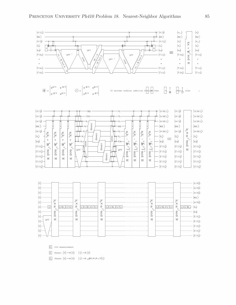
Princeton University Ph410 Problem 18. Nearest-Neighbor Algorithms 85
kx + 2mmod N, -N
j
i2
kx + 2m
mod N
ji
2
swap swap
QFT
QFT
QFT -1
QFT -1
L R
x(i)j+1
L(b)f
MS
ki
kx
0(b)f
L(c)f
ki
kx
0(c)f
MS1(b)f
kx
MS
kx
kx
1(c)f
If another modular addition follows then = = null, else = L R=eip/4 e-ip/4
e-ip/4 eip/4
e-ip/4
e-ip/4eip/4
eip/4
=
x(i)j x(i)j+1
MS
x(i)j
MS + N
kx - 2m
mod N
ji
2
xj+1
L(b)f
MS
xj
ki
kx
0(b)f
xj+1
L(c)f
MS
xj
ki
kx
0(c)f
1(b)f 1(c)f
kx + 2 a
mod N
ji
2
L R
cswap
cswap
cswap
cswap
mesh
mesh
4(0)f
MS
ki
kx
0(0)f
1(0)f
2(0)f
3(0)fQFT -1 QFT
4(0)f
MS
ki
kx
0(0)f
1(0)f
2(0)f
3(0)f
x0
x1
x2
x3
ki
kx
MS x3
x2
x1
MS
x0
ki
kx
4(0)f
MS
ki
kx
0(0)f
1(0)f
2(0)f
3(0)f
4(0)f
MS
ki
kx
0(0)f
1(0)f
2(0)f
3(0)f
x0 k
i + 2m
mod N
0i
2
x1 k
i + 2m
mod N
1i
2
x2 k
i + 2m
mod N
2i
2
x3 k
i + 2m
mod N
3i
2
x0 k
i - 2 m
mod N
0i
2(
) -1
x1 k
i - 2 m
mod N
1i
2(
) -1
x2 k
i - 2 m
mod N
2i
2(
) -1
x3 k
i - 2 m
mod N
3i
2(
) -1
3x(i)
2x(i)
1x(i)
0x(i)
3x(i)
2x(i)
1x(i)
0x(i)
3x(i+1)
2x(i+1)
1x(i+1)
0x(i+1)
3x(i+1)
2x(i+1)
1x(i+1)
0x(i+1)
ki m
mod N
i2
QFT
0
0
0
0
1
0
0
0
0
0
0
0
M i
R
Z3
4(0)f
MS
k8
kx
0(0)f
1(0)f
2(0)f
3(0)f
3x(8)
2x(8)
1x(8)
0x(8)
k0
mmod N
02
k1
mmod N
12
k2
mmod N
22
k6
mmod N
62
k7
mmod N
72H H M 1 R Z1H H R H Z2 H M 3 R H Z6 H M 7 R H Z1 H M 8M 2
ith measurement
Reset:
eipM 3M 2M 1/23
10 0 0
0 0 1 1Phase:
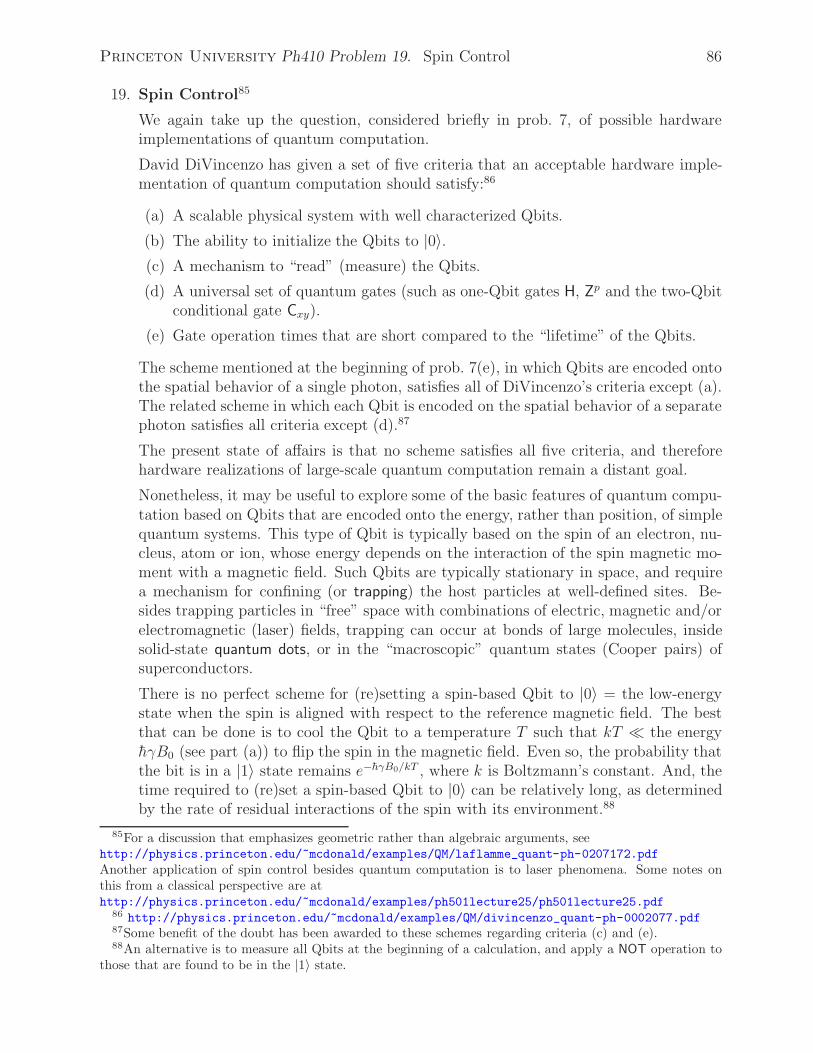
Princeton University Ph410 Problem 19. Spin Control 86
19. Spin Control85
We again take up the question, considered briefly in prob. 7, of possible hardwareimplementations of quantum computation.
David DiVincenzo has given a set of five criteria that an acceptable hardware imple-mentation of quantum computation should satisfy:86
(a) A scalable physical system with well characterized Qbits.
(b) The ability to initialize the Qbits to |0〉.(c) A mechanism to “read” (measure) the Qbits.
(d) A universal set of quantum gates (such as one-Qbit gates H, Zp and the two-Qbitconditional gate Cxy).
(e) Gate operation times that are short compared to the “lifetime” of the Qbits.
The scheme mentioned at the beginning of prob. 7(e), in which Qbits are encoded ontothe spatial behavior of a single photon, satisfies all of DiVincenzo’s criteria except (a).The related scheme in which each Qbit is encoded on the spatial behavior of a separatephoton satisfies all criteria except (d).87
The present state of affairs is that no scheme satisfies all five criteria, and thereforehardware realizations of large-scale quantum computation remain a distant goal.
Nonetheless, it may be useful to explore some of the basic features of quantum compu-tation based on Qbits that are encoded onto the energy, rather than position, of simplequantum systems. This type of Qbit is typically based on the spin of an electron, nu-cleus, atom or ion, whose energy depends on the interaction of the spin magnetic mo-ment with a magnetic field. Such Qbits are typically stationary in space, and requirea mechanism for confining (or trapping) the host particles at well-defined sites. Be-sides trapping particles in “free” space with combinations of electric, magnetic and/orelectromagnetic (laser) fields, trapping can occur at bonds of large molecules, insidesolid-state quantum dots, or in the “macroscopic” quantum states (Cooper pairs) ofsuperconductors.
There is no perfect scheme for (re)setting a spin-based Qbit to |0〉 = the low-energystate when the spin is aligned with respect to the reference magnetic field. The bestthat can be done is to cool the Qbit to a temperature T such that kT � the energyhγB0 (see part (a)) to flip the spin in the magnetic field. Even so, the probability thatthe bit is in a |1〉 state remains e−hγB0/kT , where k is Boltzmann’s constant. And, thetime required to (re)set a spin-based Qbit to |0〉 can be relatively long, as determinedby the rate of residual interactions of the spin with its environment.88
85For a discussion that emphasizes geometric rather than algebraic arguments, seehttp://physics.princeton.edu/~mcdonald/examples/QM/laflamme_quant-ph-0207172.pdfAnother application of spin control besides quantum computation is to laser phenomena. Some notes onthis from a classical perspective are athttp://physics.princeton.edu/~mcdonald/examples/ph501lecture25/ph501lecture25.pdf
86 http://physics.princeton.edu/~mcdonald/examples/QM/divincenzo_quant-ph-0002077.pdf87Some benefit of the doubt has been awarded to these schemes regarding criteria (c) and (e).88An alternative is to measure all Qbits at the beginning of a calculation, and apply a NOT operation to
those that are found to be in the |1〉 state.
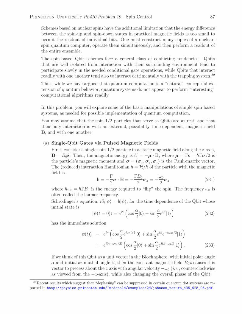
Princeton University Ph410 Problem 19. Spin Control 87
Schemes based on nuclear spins have the additional limitation that the energy differencebetween the spin-up and spin-down states in practical magnetic fields is too small topermit the readout of individual bits. One must construct many copies of a nuclear-spin quantum computer, operate them simultaneously, and then perform a readout ofthe entire ensemble.
The spin-based Qbit schemes face a general class of conflicting tendencies. Qbitsthat are well isolated from interaction with their surrounding environment tend toparticipate slowly in the needed conditional gate operations, while Qbits that interactreadily with one another tend also to interact detrimentally with the trapping system.89
Thus, while we have argued that quantum computation is a “natural” conceptual ex-tension of quantum behavior, quantum systems do not appear to perform “interesting”computational algorithms readily.
In this problem, you will explore some of the basic manipulations of simple spin-basedsystems, as needed for possible implementation of quantum computation.
You may assume that the spin-1/2 particles that serve as Qbits are at rest, and thattheir only interaction is with an external, possibility time-dependent, magnetic fieldB, and with one another.
(a) Single-Qbit Gates via Pulsed Magnetic Fields
First, consider a single spin-1/2 particle in a static magnetic field along the z-axis,B = B0z. Then, the magnetic energy is U = −μ · B, where μ = Γs = hΓσ/2 isthe particle’s magnetic moment and σ = (σx,σy,σz) is the Pauli-matrix vector.The (reduced) interaction Hamiltonian h = H/h of the particle with the magneticfield is
h = −Γ
2σ · B = −ΓB0
2σz = −ω0
2σz (231)
where hω0 = hΓB0 is the energy required to “flip” the spin. The frequency ω0 isoften called the Larmor frequency.
Schrodinger’s equation, i∂t|ψ〉 = h|ψ〉, for the time dependence of the Qbit whoseinitial state is
|ψ(t = 0)〉 = eiγ(cos
α
2|0〉 + sin
α
2eiβ|1〉
)(232)
has the immediate solution
|ψ(t)〉 = eiγ(cos
α
2eiω0t/2|0〉 + sin
α
2eiβe−iω0t/2|1〉
)
= ei(γ+ω0t/2)(cos
α
2|0〉 + sin
α
2ei(β−ω0t)|1〉
). (233)
If we think of this Qbit as a unit vector in the Bloch sphere, with initial polar angleα and initial azimuthal angle β, then the constant magnetic field B0z causes thisvector to precess about the z axis with angular velocity−ω0 (i.e., counterclockwiseas viewed from the +z-axis), while also changing the overall phase of the Qbit.
89Recent results which suggest that “dephasing” can be suppressed in certain quantum dot systems are re-ported in http://physics.princeton.edu/~mcdonald/examples/QM/johnson_nature_435_925_05.pdf

Princeton University Ph410 Problem 19. Spin Control 88
The magnetic field has no effect on our interpretation of this Qbit in the [0,1]basis, so it is convenient to adopt a viewpoint that renders this Qbit as, in effect,constant. This can be done by viewing the Qbit from a frame that rotates aboutthe z axis of Bloch space with angular velocity −ω0.
We now want to transform the Qbit in various ways, always interpreting the effectof the transformations in the rotating frame. For example, a general unitary 1-Qbit operation can be represented by a product of 3 rotations plus an overallphase change. To perform a rotation of the Qbit by angle λ about some axis u(in the rotating frame), we can use the insights of eqs. (231)-(233) and turn ona uniform magnetic field Buu (in the rotating frame), which will cause the Qbitto precess about the u with angular velocity ωu = ΓBu. So, if we turn off thefield Bu after time t = θ/ωu, we will have accomplished the desired rotation (withrespect to the rotating frame). The quantity ωu is often called the Rabi frequency.
We can establish a formal relation between the lab- and rotating-frame descrip-tions by considering eq. (232) to be the rotating-frame Qbit |ψrot〉. Using eq. (233)for the lab-frame version, |ψlab〉 of this Qbit, we have
|ψlab〉 = eiω0t/2
⎛⎝ 1 0
0 e−iω0t
⎞⎠ |ψrot〉 = eiω0t/2σ−ω0t/π
z |ψrot〉
= eiω0t/2e−iω0t/2eiω0t2
σz |ψrot〉 = eiω0t2
σz |ψrot〉, (234)
recalling eqs. (54)-(55).
We can deduce a version of Schrodinger’s equation for the rotating-frame Qbit|ψrot〉 as follows,
i∂t|ψlab〉 = i∂tei
ω0t
2σz |ψrot〉 = −ω0
2σze
iω0t
2σz |ψrot〉 + ei
ω0t
2σz(i∂t|ψrot〉)
= hlab|ψlab〉 = hlabei
ω0t
2σz |ψrot〉, (235)
which can be rearranged as90
i∂t|ψrot〉 = e−iω0t2
σz
(hlab +
ω0
2σz
)ei
ω0t2
σz |ψrot〉 = hrot|ψrot〉. (236)
Now consider the case that the lab-frame magnetic field includes a static fieldalong the z-axis, B0z, and a time-dependent field Buu that rotates (precesses)about the z-axis with angular velocity −ω0,
B = B0z+Bu[ux(cosω0t x− sinω0t y)+uy(sinω0t x+cosω0t y)+uz z], (237)
where the components (ux, uy, uz) of unit vector u are for time t = 0 (and henceare the components of u in the rotating frame).
Show that the Hamiltonian in the rotating frame has the time-independent form
hrot = −ωu2
u · σ, where ωu = ΓBu. (238)
90Experts will recognize eqs. (234) and (236) as an example of the effect of a basis transformation by aunitary operator U, namely |ψ′〉 = U|ψ〉 and h′ = U−1hU.
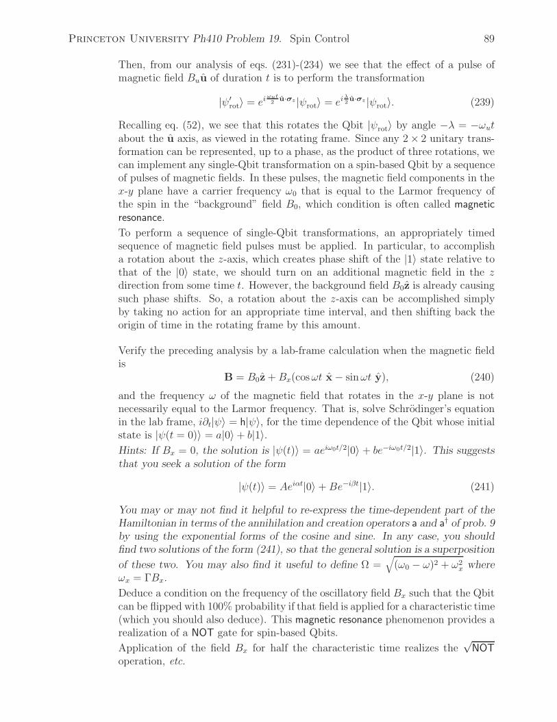
Princeton University Ph410 Problem 19. Spin Control 89
Then, from our analysis of eqs. (231)-(234) we see that the effect of a pulse ofmagnetic field Buu of duration t is to perform the transformation
|ψ′rot〉 = ei
ωut2
u·σz |ψrot〉 = eiλ2u·σz |ψrot〉. (239)
Recalling eq. (52), we see that this rotates the Qbit |ψrot〉 by angle −λ = −ωutabout the u axis, as viewed in the rotating frame. Since any 2 × 2 unitary trans-formation can be represented, up to a phase, as the product of three rotations, wecan implement any single-Qbit transformation on a spin-based Qbit by a sequenceof pulses of magnetic fields. In these pulses, the magnetic field components in thex-y plane have a carrier frequency ω0 that is equal to the Larmor frequency ofthe spin in the “background” field B0, which condition is often called magneticresonance.
To perform a sequence of single-Qbit transformations, an appropriately timedsequence of magnetic field pulses must be applied. In particular, to accomplisha rotation about the z-axis, which creates phase shift of the |1〉 state relative tothat of the |0〉 state, we should turn on an additional magnetic field in the zdirection from some time t. However, the background field B0z is already causingsuch phase shifts. So, a rotation about the z-axis can be accomplished simplyby taking no action for an appropriate time interval, and then shifting back theorigin of time in the rotating frame by this amount.
Verify the preceding analysis by a lab-frame calculation when the magnetic fieldis
B = B0z +Bx(cosωt x − sinωt y), (240)
and the frequency ω of the magnetic field that rotates in the x-y plane is notnecessarily equal to the Larmor frequency. That is, solve Schrodinger’s equationin the lab frame, i∂t|ψ〉 = h|ψ〉, for the time dependence of the Qbit whose initialstate is |ψ(t = 0)〉 = a|0〉 + b|1〉.Hints: If Bx = 0, the solution is |ψ(t)〉 = aeiω0t/2|0〉 + be−iω0t/2|1〉. This suggeststhat you seek a solution of the form
|ψ(t)〉 = Aeiαt|0〉 +Be−iβt|1〉. (241)
You may or may not find it helpful to re-express the time-dependent part of theHamiltonian in terms of the annihilation and creation operators a and a† of prob. 9by using the exponential forms of the cosine and sine. In any case, you shouldfind two solutions of the form (241), so that the general solution is a superposition
of these two. You may also find it useful to define Ω =√
(ω0 − ω)2 + ω2x where
ωx = ΓBx.
Deduce a condition on the frequency of the oscillatory field Bx such that the Qbitcan be flipped with 100% probability if that field is applied for a characteristic time(which you should also deduce). This magnetic resonance phenomenon provides arealization of a NOT gate for spin-based Qbits.
Application of the field Bx for half the characteristic time realizes the√
NOToperation, etc.

Princeton University Ph410 Problem 19. Spin Control 90
(b) Two-Qbit Coupling
The interaction of two magnetic dipoles μ1 and μ2 whose separation is r12 leadsto a configuration energy,
U12 =μ1 · μ2 − 3(μ1 · r12)(μ2 · r12)
r312
. (242)
In many realizations of spin-based Qbits, the 2-Qbit interaction energy is wellapproximated by the simpler form
U12 =μ1 · μ2
r312
. (243)
The corresponding lab-frame interaction Hamiltonian can be written
h12 =ω12
2σ(1) ·σ(2), (244)
where the coupling strength ω12 is (relatively) large only for nearest-neighborQbits. This Hamiltonian has the same functional form with respect to, say, thefirst Qbit as does the interaction (231) of that Qbit with an external magneticfield. Therefore, if we view the two Qbits in their respective rotating frames, theeffect of the Hamiltonian (244) during a time t is to evolve the 2-Qbit state |ψR〉12
according to91
|ψ′rot〉12 = e−i
ω12t
2σ(1)·σ(2)|ψrot〉12
= e−iω12t
2σ
(1)x σ
(2)x e−i
ω12t
2σ
(1)y σ
(2)y e−i
ω12t
2σ
(1)z σ
(2)z |ψrot〉12. (245)
Show that the interaction of two Qbits for a time t = π/2ω12 according to eq. (244)performs the SWAP operation S12 to within a phase.
This result gives an additional perspective as to why a collection of spins is notspontaneously a “useful” quantum computer. Namely, the dipole-dipole couplingbetween any pair of spins results in continual swapping of their states. The rate ofswapping falls off with the distance between the pair, but at some rate each spinswaps its state with all other spins. The overall behavior is somewhat “chaotic”.
A possible way to gain control over the swapping is to place each spin in a “trap”which is fairly well isolated from all other spins. Then, when an interaction isdesired between a particular pair of nearest-neighbor spins, the “trapping” forcesare adjusted to bring those two spins closer together. After a time sufficient for thedesired interaction to occur, the spins are returned to their (relatively) isolatedinitial positions.
As we discussed at the end of prob. 12, a SWAP operation is not a sufficientbuilding block for all 2-Qbit interactions. However, if we allow a pair of spins tointeract for only 1/2 the time needed for a SWAP operation, we will have achieved
91The second form of eq. (245) clarifies the meaning of the exponential of the product of two Pauli matrices
that act on different Qbits. That is, eiασ(1)j σ
(2)j = cosα I + i sinα σ(1)
j σ(2)j for j = x, y, z, but eiασ(1)·σ(2)
does not equal cosα I + i sinα σ(1) · σ(2).

Princeton University Ph410 Problem 19. Spin Control 91
the√
S12 operation, which is a universal 2-Qbit gate. Thus, we have one schemewhereby, in principle, we can construct a spin-based quantum computer capableof executing any quantum algorithm.
It turns out that in some spin systems the 2-Qbit coupling is well approximatedby a further simplification of eq. (244), namely
h12 =ω12
2σ(1)z σ
(2)z , (246)
when the system is immersed in a “background” magnetic field along the z-axis.
Show that a Controlled-NOT operation C12 can be represented by the followingsequence of magnetic-field pulses (to within an overall phase),
C12 ∝ e−iπ4σ
(1)z ei
π4σ
(2)y ei
π4σ
(2)z e−i
π4σ
(1)z σ
(2)z e−i
π4σ
(2)y . (247)
Given eq. (247), we see at once that
C21 ∝ e−iπ4σ
(2)z ei
π4σ
(1)y ei
π4σ
(1)z e−i
π4σ
(1)z σ
(2)z e−i
π4σ
(1)y . (248)
The sequence of operations (247) can be given a geometrical interpretation. Recall
from eq. (52) that an operator eiφ2σj corresponds to a rotation of a Qbit in Bloch
space by angle −φ about axis j.
i. The first operation, e−iπ4σ
(2)y , rotates the target Qbit |ψ〉2 by +90◦ about the
y2 axis. This means that |0〉2 rotates from z2 to x2, while |1〉2 rotates from−z2 to −x2.
|ψ〉2 Initial Direction
direction after step i
|0〉 z2 x2
|1〉 −z2 −x2
(249)
ii. The second operation, e−iπ4σ
(1)z σ
(2)z , provides the key conditional action. It
rotates Qbit 2 by +90◦ about the z2 axis if Qbit 1 is |0〉, but it rotates Qbit2 by −90◦ about the z2 axis if Qbit 1 is |1〉. Algebraically,
e−iπ4σ
(1)z σ
(2)z =
I − iσ(1)z σ
(2)z√
2=
⎧⎪⎨⎪⎩
I−iσ(2)z√
2= e−i
π4σ
(2)z if |ψ〉1 = |0〉1,
I+iσ(2)z√
2= ei
π4σ
(2)z if |ψ〉1 = |1〉1.
(250)
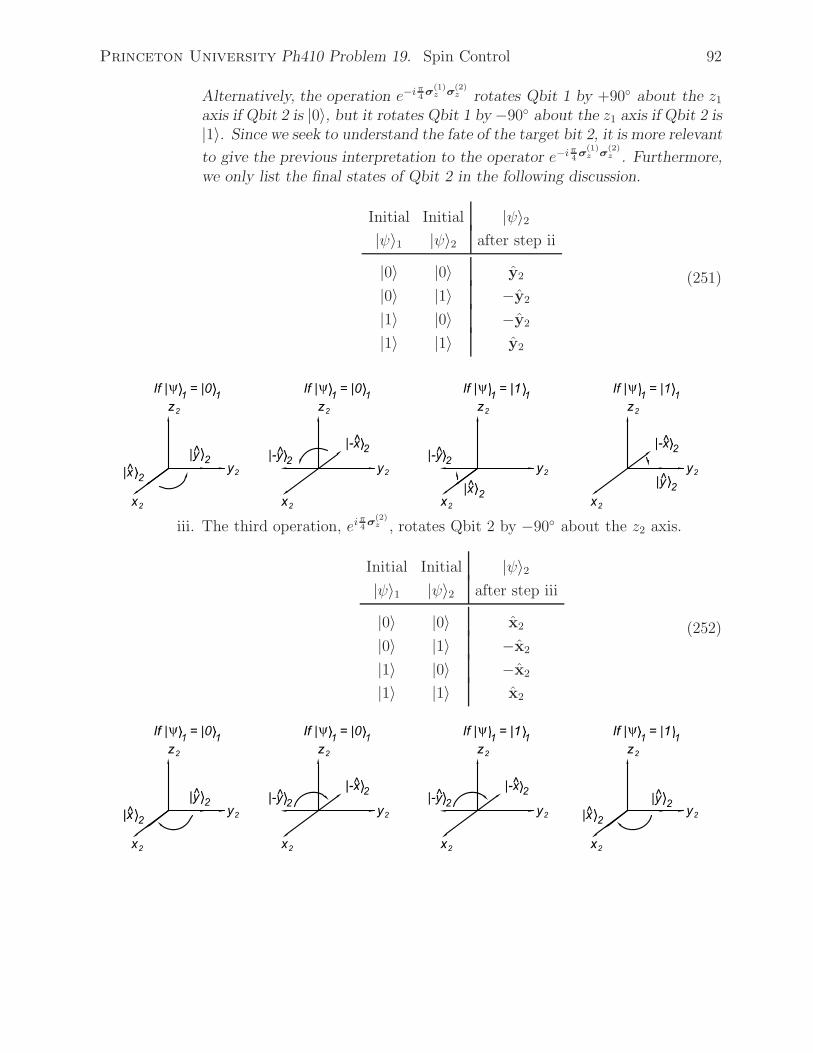
Princeton University Ph410 Problem 19. Spin Control 92
Alternatively, the operation e−iπ4σ
(1)z σ
(2)z rotates Qbit 1 by +90◦ about the z1
axis if Qbit 2 is |0〉, but it rotates Qbit 1 by −90◦ about the z1 axis if Qbit 2 is|1〉. Since we seek to understand the fate of the target bit 2, it is more relevant
to give the previous interpretation to the operator e−iπ4σ
(1)z σ
(2)z . Furthermore,
we only list the final states of Qbit 2 in the following discussion.
Initial Initial |ψ〉2|ψ〉1 |ψ〉2 after step ii
|0〉 |0〉 y2
|0〉 |1〉 −y2
|1〉 |0〉 −y2
|1〉 |1〉 y2
(251)
iii. The third operation, eiπ4σ
(2)z , rotates Qbit 2 by −90◦ about the z2 axis.
Initial Initial |ψ〉2|ψ〉1 |ψ〉2 after step iii
|0〉 |0〉 x2
|0〉 |1〉 −x2
|1〉 |0〉 −x2
|1〉 |1〉 x2
(252)

Princeton University Ph410 Problem 19. Spin Control 93
iv. The fourth operation, eiπ4σ
(2)y , rotates Qbit 2 by −90◦ about the y2 axis. This
restores Qbit 2 to its initial direction if Qbit 1 is |0〉, but inverts Qbit 2 ifQbit 1 is |1〉.
Initial Initial |ψ〉2|ψ〉1 |ψ〉2 after step iv
|0〉 |0〉 z2
|0〉 |1〉 −z2
|1〉 |0〉 −z2
|1〉 |1〉 z2
(253)
It looks like we are done, but if Qbit 1 was not in a basis state, things areslightly confused. This is fixed by the final step.
v. The fifth operation, e−iπ4σ
(1)z , rotates Qbit 1 by +90◦ about the z1 axis. This
tidies up the phases of the Qbits, as you will demonstrate in the algebraicexercise assigned above, so the complete set of steps performs the desiredControlled-NOT to within an overall phase.
Initial Initial Final Final
|ψ〉1 |ψ〉2 |ψ〉1 |ψ〉2|0〉 |0〉 |0〉 |0〉|0〉 |1〉 |0〉 |1〉|1〉 |0〉 |1〉 |1〉|1〉 |1〉 |1〉 |0〉
(254)
This analysis could have been carried out in more detail, keeping track ofthe phase of Qbit 1 at each step. But then there would be little differencebetween the “geometric” approach and an algebraic approach.
Give a similar “geometric” argument to show how the operation
e−iπ4σ(1)·σ(2)
= e−iπ4σ
(1)x ·σ(2)
x e−iπ4σ
(1)y ·σ(2)
y e−iπ4σ
(1)z ·σ(2)
z (255)
swaps Qbits 1 and 2.
It suffices to show that this operation performs a SWAP on each of the 2-Qbitbasis states |0〉1|0〉2, |0〉1|1〉2, |1〉1|0〉2 and |1〉1|1〉2 up to a phase which varies from

Princeton University Ph410 Problem 19. Spin Control 94
state to state. Your earlier algebraic argument shows that the phase change isactually independent of the 2-Qbit state.
The first step of operation (255) is e−iπ4σ
(1)z σ
(2)z which performs conditional rota-
tions by ±90◦ about the z-axes. Since all of our initial states are aligned alongthe z axes, the first step merely changes the phases of the initial states, but nottheir directions. In the geometric view, this step has no effect.
The second step of operation (255) is e−iπ4σ
(1)y σ
(2)y which performs a conditional
rotation of bit 2 by ±90◦ about the y2-axis depending on the state of bit 1 asprojected onto the y1-axis (or equivalently, a conditional rotation of bit 1 by ±90◦
about the y1-axis depending on the state of bit 2 as projected onto the y2-axis).This will result in the initial states, which were aligned along the z axes, beingtransformed into various combinations of states readily expressed with one bitalong its x-axis and the other bit along its y-axis.
The third step of operation (255) is e−iπ4σ
(1)x σ
(2)x which performs conditional rota-
tions ±90◦ about the x-axes. Since the input states to this operation are simplyexpressed with one of the two bits aligned along its x-axis, it is relatively straight-forward to keep track of this step.
Here we illustrate the case when the initial state is |0〉1|0〉2, which can be expressedin various equivalent ways,
|ψ0〉 = |0〉1|0〉2 = |z〉1|z〉2 =|y〉1 + | − y〉1√
2|z〉2 = |z〉1 |y〉2 + | − y〉2√
2. (256)
To determine the rotation of the second Qbit by the operation e−iπ4σ
(1)y σ
(2)y , which
is conditional on the state of the first Qbit, we need the first Qbit to be described
relative to the y1 axis. Recalling from eq. (52) that the operator e−iπ4σ
(2)y is a
rotation of bit 2 by +90◦ about the y2-axis, we learn that when bit 1 is |y〉1 bit2 is rotated from |z〉2 to |x〉2, and that when bit 1 is | − y〉1 bit 2 is rotated from|z〉2 to | − x〉2.
That is,
e−iπ4σ
(1)y σ
(2)y |0〉1|0〉2 = e−i
π4σ
(1)y σ
(2)y|y〉1 + | − y〉1√
2|z〉2 =
|y〉1|x〉2 + | − y〉1| − x〉2√2
.
(257)Alternatively, we could consider the 2nd bit to be the control bit, in which casethe transformation can be written
|0〉1|0〉2 = |z〉1 |y〉2 + | − y〉2√2
→ |x〉1|y〉2 + | − x〉1| − y〉2√2
, (258)

Princeton University Ph410 Problem 19. Spin Control 95
which you may wish to verify is actually the same as eq. (257).
To understand the effect of the conditional operation e−iπ4σ
(1)x σ
(2)x , one of the two
bits should be expressed in terms of its projections onto the x-axis. Both eqs. (257)and (258) are already of the desired form, so we can use either. Specifically, thetransformation of eq. (257) is that when bit 2 is |x〉2 bit 1 is rotated from |y〉1 to|z〉1, and that when bit 2 is | − x〉2 bit 1 is rotated from | − y〉1 to |z〉1.
Then,
e−iπ4σ
(1)x σ
(2)x|y〉1|x〉2 + | − y〉1| − x〉2√
2=
|z〉1|x〉2 + |z〉1| − x〉2√2
= |0〉1|0〉2, (259)
as expected for SWAP|0〉1|0〉2.
In systems where the spin-spin coupling is well described by the Hamiltonian(246), so that the corresponding time evolution of a pair of spins is
|ψ′rot〉12 = e−i
ω12t2
σ(1)z σ
(2)z |ψrot〉12, (260)
there is another way to arrange that this interaction is effective only during spec-ified time intervals. Namely, any interval in which it is desired that there be nonet effect of the spin-spin coupling, a pair of magnetic pulses can be applied at thebeginning and middle of the interval such that the evolution of the spin during thefirst half interval is reversed during the second half interval. This is a quantumcomputer version of the spin echo technique.92
The formal basis of this technique are the identities,
σxσzσx = σyσzσy = −σz, and σx = −ieiπ2σx, σy = −ieiπ
2σy , (261)
which imply that
eiπ2σ
(1)x e−i
ω12t2
σ(1)z σ
(2)z ei
π2σ
(1)x = −σ(1)
x e−iω12t
2σ
(1)z σ
(2)z σ(1)
x
= −σ(1)x
(cos
ω12t
2− i sin
ω12t
2σ(1)z σ
(2)z
)σ(1)x
= −(cos
ω12t
2+ i sin
ω12t
2σ(1)z σ
(2)z
)
= −eiω12t2
σ(1)z σ
(2)z , (262)
92 http://physics.princeton.edu/~mcdonald/examples/QM/hahn_pr_80_580_50.pdf

Princeton University Ph410 Problem 19. Spin Control 96
and therefore,
e−iω12t
2σ
(1)z σ
(2)z ei
π2σ
(1)x e−i
ω12t2
σ(1)z σ
(2)z ei
π2σ
(1)x = −I. (263)
We could also have used the operation eiπ2σx at the middle and end of the interval
to cancel the effect of the spin-spin coupling during that interval. Or, we couldhave used the operation ei
π2σy instead of ei
π2σx . Or, we could have applied the
magnetic pulses to spin 2 rather than to spin 1, etc.

Princeton University Ph410 Problem 20. Dephasing 97
20. Dephasing93
In prob. 19 we alluded to the difficulty that Qbits interact with their environment inways that are detrimental to quantum computation. This problem explores methodsof formalizing our understanding of these difficulties.
The situation is a version of Schrodinger’s cat: we desire that our Qbits remain ina pure quantum state inside our quantum computer, at least for the duration of thecalculation. But the worry is that these ideal quantum states do not survive that long,and are converted into Cbits even before we “look” at the results of our computation.
The interactions of the Qbits with their environment may perform some kind of “mea-surement” on them, the results of which we do not know in detail because we haven’tyet observed the Qbits ourselves. So, we desire a description of quantum states thatincludes the possibility that they are in one of several possible basis states as a resultof interactions beyond our control, as well as the possibility that the Qbits are still ina coherent superposition of basis states as we have assumed in this course until now.
Such a description was provided independently(?) in 1927 by Landau and by vonNeumann, and is based on the concept of the density operator, also called the densitymatrix.
Wave Function of a Pure State
If a quantum system is in an idealized pure state, we have characterized this by a wavefunction
|ψ〉 =∑j
ψj|j〉, (2)
that is a weighted sum of basis states |j〉. The time evolution of state |ψ〉 has beendescribed by a unitary transformation U(t, t′) such that
|ψ(t′)〉 = U(t, t′)|ψ(t)〉. (84)
If the state |ψ〉 is observed via a (hermitian) measurement operator M whose eigenvec-tors are the basis states |j〉 with corresponding eigenvalues mj, then we can write
M =∑j
Mj =∑j
mj · Pj =∑j
mj · |j〉〈j|, (81)
and the probability that the result of the measurement is that state |ψ〉 is found inbasis state |j〉 is
Pj = 〈ψ|P†jPj|ψ〉 = 〈ψ|Pj|ψ〉 = 〈ψ|j〉〈j|ψ〉 = |〈j|ψ〉|2 . (78)
The probable value (or expectation value) of variable m for state |ψ〉 is thus
〈m〉 =∑j
mjPj =∑j
mj〈ψ|Pj |ψ〉 = 〈ψ|∑j
mj · Pj|ψ〉 = 〈ψ|M|ψ〉. (82)
93Problem 20 is covered in sec. 2.4 and chap. 8 of Nielsen and Chuang.
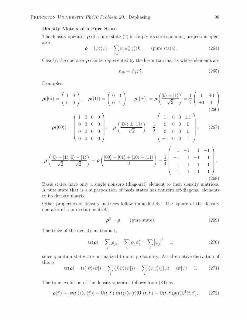
Princeton University Ph410 Problem 20. Dephasing 98
Density Matrix of a Pure State
The density operator ρ of a pure state (2) is simply its corresponding projection oper-ator,
ρ = |ψ〉〈ψ| =∑j,k
ψjψ�k|j〉〈k| (pure state). (264)
Clearly, the operator ρ can be represented by the hermitian matrix whose elements are
ρjk = ψjψ�k. (265)
Examples:
ρ(|0〉) =
⎛⎝ 1 0
0 0
⎞⎠ , ρ(|1〉) =
⎛⎝ 0 0
0 1
⎞⎠ , ρ(|±〉) = ρ
(|0〉 ± |1〉√2
)=
1
2
⎛⎝ 1 ±1
±1 1
⎞⎠ ,
(266)
ρ(|00〉) =
⎛⎜⎜⎜⎜⎜⎜⎝
1 0 0 0
0 0 0 0
0 0 0 0
0 0 0 0
⎞⎟⎟⎟⎟⎟⎟⎠, ρ
( |00〉 ± |11〉√2
)=
1
2
⎛⎜⎜⎜⎜⎜⎜⎝
1 0 0 ±1
0 0 0 0
0 0 0 0
±1 0 0 1
⎞⎟⎟⎟⎟⎟⎟⎠, (267)
ρ
( |0〉 + |1〉√2
|0〉 − |1〉√2
)= ρ
(|00〉 − |01〉 + |10〉 − |11〉2
)=
1
4
⎛⎜⎜⎜⎜⎜⎜⎝
1 −1 1 −1
−1 1 −1 1
1 −1 1 −1
−1 1 −1 1
⎞⎟⎟⎟⎟⎟⎟⎠.
(268)Basis states have only a single nonzero (diagonal) element to their density matrices.A pure state that is a superposition of basis states has nonzero off-diagonal elementsto its density matrix.
Other properties of density matrices follow immediately: The square of the densityoperator of a pure state is itself,
ρ2 = ρ (pure state). (269)
The trace of the density matrix is 1,
tr(ρ) =∑j
ρjj =∑j
ψjψ�j =
∑j
∣∣∣ψj∣∣∣2 = 1, (270)
since quantum states are normalized to unit probability. An alternative derivation ofthis is
tr(ρ) = tr(|ψ〉〈ψ|) =∑j
〈j|ψ〉〈ψ|j〉 =∑j
〈ψ|j〉〈j|ψ〉 = 〈ψ|ψ〉 = 1. (271)
The time evolution of the density operator follows from (84) as
ρ(t′) = |ψ(t′)〉〈ψ(t′)| = U(t, t′)|ψ(t)〉〈ψ(t)|U†(t, t′) = U(t, t′)ρ(t)U†(t, t′). (272)
Princeton University Ph410 Problem 20. Dephasing 99
The probability that state |ψ〉 is found in basis state |j〉 as the result of a measurementfollows from (78) as
Pj = |〈j|ψ〉|2 = 〈ψ|j〉〈j|ψ〉 = 〈j|ψ〉〈ψ|j〉 = 〈j|j〉〈j|ψ〉〈ψ|j〉 =∑k
〈k|j〉〈j|ψ〉〈ψ|k〉= tr(|j〉〈j|ψ〉〈ψ|) = tr(Pjρ), (273)
which is a special case of the general result for an operator O that
〈ψ|O|ψ〉 = tr(Oρ). (274)
The expectation value 〈m〉 for a measurement of state |ψ〉 using operator M =∑jmj ·Pj
of eq. (79) follows from eqs. (83) and (274) as
〈m〉 =∑j
mj〈ψ|Pj|ψ〉 =∑j
mjtr(Pjρ) = tr(Mρ). (275)
Density Matrix of a Mixed State
These results show that the density-matrix description of a pure quantum state recoversall the features of the usual description. However, there does not yet appear to be anyadvantage to the use of density matrices. That advantage lies in the ease with whichthe density-matrix description can be extended to include so-called mixed states inwhich the quantum state is one of a set of pure states |ψi〉 with probability Pi, wherethe total probability is, of course, unity:
∑i Pi = 1. In this case, we define
ρ =∑i
Pi|ψi〉〈ψi| =∑i
Piρi (mixed state). (276)
We readily set that the mixed-state density matrix (276) obeys all of the properties(270)-(275). However,
ρ2 = ρ (mixed state), (277)
which provides a means of determining whether a given density matrix describes a purestate or a mixed state.
Example: A 50:50 mixture of states |00〉 and |11〉 has density matrix
ρ =1
2
⎛⎜⎜⎜⎜⎜⎜⎝
1 0 0 0
0 0 0 0
0 0 0 0
0 0 0 1
⎞⎟⎟⎟⎟⎟⎟⎠. (278)
A mixture of basis states has no off-diagonal elements in its density matrix.
Example: A 50:50 mixture of states |0〉 and |1〉 has the same density matrix as a 50:50mixture of states |+〉 and |−〉. From eq. (266) we have,
ρ =ρ(|0〉) + ρ(|1〉)
2=ρ(|+〉) + ρ(|−〉)
2=
1
2
⎛⎝ 1 0
0 1
⎞⎠ =
I
2. (279)
Princeton University Ph410 Problem 20. Dephasing 100
Indeed, the rotation (46) of basis states |0〉 and |1〉 by angle θ about the y-axis in Blochspace leads to the new basis states cos θ
2|0〉 − sin θ
2|1〉 and sin θ
2|0〉 + cos θ
2|1〉. Hence, a
50:50 mixture of these new basis states also has density matrix (279).
A historic debate about the meaning of the quantum wave functions concerns whetherthey reflect that Nature is intrinsically probabilistic or that the probabilities merelyreflect our ignorance of some underlying well-defined “reality”. We argue that a purestate is one for which probabilities are intrinsic.94 In contrast, a mixed state (276) canbe regarded as actually being in one of its component pure states |ψi〉, but we don’tknow which.95 The probabilities Pi in eq. (276) summarize our ignorance/knowledgeof which pure states are present, while the coefficients ψj in eq. (2) represent intrinsicprobabilities (strictly, probability amplitudes) as to what can be observed of the purestate |ψ〉.Mixed states and their density-matrix description are therefore useful in quantumstatistical mechanics in which we are ignorant of details of the state of our system orensemble of systems.
Density Matrix of a Composite System
The density-matrix description is also useful when dealing with a system for which wehave different qualities of information about its component subsystems.
Consider a system with two subsystems A and B for which the density matrix of thewhole system is ρAB . If our knowledge of system B is limited, we may wish to considerwhat we can say about system A only. That is, we desire the density matrix ρA.
The claim is that the appropriate procedure is to calculate
ρA = trB(ρAB), (280)
where the trace over subsystem B can be accomplished with the aid of the definition
trB(|A1B1〉〈A2B2|) = trB(|A1〉〈A2| ⊗ |B1〉〈B2|) = |A1〉〈A2| trB(|B1〉〈B2|)= |A1〉〈A2| 〈B1|B2〉, (281)
recalling eq. (271).
If subsystems A and B have no nontrivial couplings, then ρAB = ρA ⊗ ρB, so thattr(ρAB) = tr(ρA ⊗ ρB) = ρA tr(ρB) = ρA, as expected.
Of greater interest is the case when subsystems A and B are entangled. For example,consider the entangled 2-Qbits states described by the righthand case in eq. (267). Toapply eq. (281) it is easier to rewrite the density matrix (267) as a density operator,
ρAB
( |00〉 ± |11〉√2
)=
|00〉 ± |11〉√2
〈00| ± 〈11|√2
=|00〉〈00| ± |00〉〈11| ± |11〉〈00| + |11〉〈11|
2.
(282)
94For a recent review of the Kochen-Specker theorem that a quantum-mechanical spin-1/2 state cannot“really” have simultaneous definite values of its spin vector along three orthogonal axes, seehttp://physics.princeton.edu/~mcdonald/examples/QM/cassinello_ajp_73_272_05.pdf
95The example of eq. (279) reminds us that a given mixed-state density matrix corresponds to differentmixtures in different bases, so considerable quantum subtlety remains even for mixed states.

Princeton University Ph410 Problem 20. Dephasing 101
Then,
ρA = trB(ρAB) =|0〉〈0| 〈0|0〉 ± |0〉〈1| 〈0|1〉 ± |1〉〈0| 〈1|0〉 + |1〉〈1| 〈1|1〉
2
=|0〉〈0| + |1〉〈1|
2=
1
2
⎛⎝ 1 0
0 1
⎞⎠ =
I
2. (283)
This noteworthy result helps us understand why Alice could not extract any infor-mation about Bob’s observations of the second Qbit of an entangled, but spatiallyseparated 2-Qbit system, as considered in prob. 6(b), by her observation of the firstQbit. Since the two Qbits are spatially separated, Alice is ignorant of the state ofBob’s Qbit, and her density-matrix description of the system is obtained by taking thetrace over the second Qbit. Although the original system was prepared as a pure state,Alice’s knowledge of that system is as if her Qbit was prepared as a 50:50 mixed stateof |0〉A and |1〉A. Nothing Bob does changes her understanding of the first Qbit, andwhen she measures it, she finds it to be a |0〉 with 50% probability, or a |1〉 with 50%probability, independent of the history of second Qbit.
Skeptics, however, might infer from the result (283) that the claim (280) is incorrect.For further justification of its validity, see Box 2.6, p. 107 of Nielsen and Chuang.96
Dephasing
As a Qbit interacts with its environment it can be perturbed in various ways. Theinformation content of the Qbit can become distributed over, or entangled with, thatenvironment, such that the quality of information of the Qbit is effectively reduced.In principle, the interactions with the environment could be reversed, and the originalinformation recovered (as in the spin-echo example given at the end of prob. 19).
But from a practical point of view, the quality of the Qbit has suffered. A quantitativemeasure of this is obtained by taking a partial trace over the environment of the densitymatrix of Qbit + environment. Analyses of this type are given the name decoherence.97
As an example, suppose the interaction of the Qbit |ψ〉 = |±〉 = (|0〉 ± |1〉)/√2 withits environment “merely” changes the relative phases of the amplitudes of |0〉 and |1〉,which causes no change in the energy of the Qbit.
Rather than construct the full density matrix of the system, we simply suppose thata phase-changing interaction with the environment can be approximated as a rotation(operator) Rz(θ) by a small angle θ that is applied to state |ψ〉. A single such interactiontransforms the density matrix of the Qbit according to eqs. (47) and (272) as,
ρ′ = Rz(θ)|ψ〉〈ψ|R†z(θ) =
1
2
⎛⎝ eiθ/2 0
0 e−iθ/2
⎞⎠⎛⎝ 1 ±1
±1 1
⎞⎠⎛⎝ e−iθ/2 0
0 eiθ/2
⎞⎠
96The density-matrix explanation of why we cannot expect controversial results from observation of one oftwo entangled subsystems could have been given by Bohr as an answer to the EPR “paradox” in 1935, butit was not. Some enthusiasts of EPR’s argument obliquely acknowledge the impact of the density matrix byreferring to it as the “destiny matrix”.
97The spokesperson for decoherence is W. Zurek,http://physics.princeton.edu/~mcdonald/examples/QM/zurek_prd_24_1516_81.pdfhttp://physics.princeton.edu/~mcdonald/examples/QM/zurek_quant-ph-0306072.pdfhttp://physics.princeton.edu/~mcdonald/examples/QM/zurek_rmp_75_715_03.pdf
Princeton University Ph410 Problem 20. Dephasing 102
=1
2
⎛⎝ 1 ±eiθ
±e−iθ 1
⎞⎠ . (284)
Typically there will be a distribution of possible phase shifts, which we approximatewith a Gaussian of variance 4λ,
P (θ) =e−θ
2/4λ
√4πλ
, so that⟨e±iθ
⟩=
1√4πλ
∫e±iθe−θ
2/4λdθ = e−λ, (285)
and hence the expectation of the density matrix (284) after one scatter is
ρ′ =1
2
⎛⎝ 1 ±e−λ
±e−λ 1
⎞⎠ . (286)
After a few times 1/λ such scatters, the phase information in the off-diagonal elementsof the density matrix has been lost, and the originally pure state has become a mixedstate,
ρ′ → 1
2
⎛⎝ 1 0
0 1
⎞⎠ =
I
2. (287)
If the state |±〉 were an input state to one of the quantum algorithms considered inprevious problems, and the dephasing (287) occurred before the main operation U ofthe algorithm has been applied, then the effect of the algorithm would be to produce
ρ′′ = Uρ′U† = UI
2U† =
I
2, (288)
just as if the algorithm had never been applied.
The major challenge in laboratory realization of quantum computation today is toincrease the dephasing time to be longer than that needed for the computation U.
(a) Show that the density matrix for a Qbit can be written as
ρ =I + r · σ
2, (289)
where r is a real 3-vector with |r| ≤ 1, and the maximum holds only if the Qbitis in a pure state. What is the unit vector r that corresponds to the pure state
|ψ〉 = eiγ[cos
α
2|0〉 + eiβ sin
α
2|1〉]? (42)
(b) In prob. 7 we considered a spatially encoded Qbit for which one path of a photon wascalled state |0〉 and another path was called state |1〉. Another type of spatiallyencoded Qbit consists of a pair (or a quartet) of quantum dots [= regions in athin silicon layer where electrodes define a potential minimum that can “trap”electrons (Earnshaw’s theorem applies in three dimensions, but not in two)]; the

Princeton University Ph410 Problem 20. Dephasing 103
states |0〉 and |1〉 are defined by the presence of an electron on one or the otherof the two quantum dots, as sketched in the figure below.98
We can also think of a spatially encoded Qbit as consisting of a pair of Qbits.Suppose that state |0〉 (|1〉) corresponds to the presence of a particle in region A(B). Then we can consider the first Qbit to have the two states |0〉A and |vac〉A,where the “vacuum” state occurs when there is no particle in region A. Similarly,the second Qbit consists of the two states |1〉B and |vac〉B. That is,
|0〉 = |0〉A|vac〉B, and |1〉 = |vac〉A|1〉B, (290)
The system AB also supports the 2-bit states |vac〉A|vac〉B and |0〉A|1〉B , but theseare not to be used for our spatially encoded Qbit.
Write down the density operator ρ for the pure states |±〉 = (|0〉±|1〉)/√2 in termsof the 2-bit states (290). What is the reduced density operator ρA = trB(ρ), thatsummarizes the knowledge of an observer who is only aware of subsystem A? Doesthis reduced density operator correspond to a pure state or to a mixed state?
(c) Recall that in the circuit for quantum teleportation, discussed in prob. 6(d), Alicemakes her measurements of bits |a〉 and |b〉 when the wave function of the systemis
|ψE〉 = α|000〉 + |100〉 + |011〉 + |111〉
2+ β
|010〉 − |110〉 + |001〉 − |101〉2
. (582)
What is the reduced density matrix of the system at this time (when |ψ〉 = |ψE〉)from Bob’s point of view? Recall that Bob has only bit |c〉 at this time, so hisknowledge of the system is described by tracing over bits |a〉 and |b〉 in the fulldensity matrix.
Your result should convince you that at this time Bob does not have knowledgeof the initial state of bit |a〉, and must await receipt of Alice’s results of hermeasurements of bits |a〉 and |b〉 of |ψE〉 before he can reconstruct the initialstate of |a〉.
98See, for example,http://physics.princeton.edu/~mcdonald/examples/QM/oi_quant-ph-0412122.pdf
Princeton University Ph410 Problem 20. Dephasing 104
(d) Other Types of Bit Errors
A more general view of interactions of a Qbit |ψ〉 with its environment begins bysupposing that initially both the Qbit and the environment are pure states, andthat the entire system is in a direct product state. Then, we write the initial stateof the environment as
|ei〉env, (291)
and the initial state of our system as
|Ψ〉 = |ei〉env ⊗ |ψ〉. (292)
The density operator ρΨ of the whole system is then
ρΨ = |Ψ〉〈Ψ| = |ei〉env ⊗ |ψ〉〈ψ| ⊗ 〈ei|env = ρenv ⊗ ρψ, (293)
where ρψ = |ψ〉〈ψ| and ρenv = |ei〉env〈ei|env.
The time evolution of the entire system is described by a unitary operator Uaccording to eq. (272),
ρ′Ψ = UρΨU† = U|ei〉env〈ei|env ⊗ ρψU†. (294)
If, as will be typical, the state of the environment is not accessible to us, we shoulddescribe the state of the Qbit |ψ′〉 = |ψ(t)〉 by the density operator ρ′
ψ that is theresult of taking the partial trace over the environment of the density operator ρΨ
of the whole system. The initial density operator ρψ is, of course, |ψ〉〈ψ|, as canbe obtained by taking the partial trace of eq. (293). The time evolution of ρ′
ψ
follows from eq. (294),
ρ′ψ = trenv(ρ
′Ψ) =
∑k
〈ek|envρ′Ψ|ek〉env =
∑k
〈ek|envU|ei〉env〈ei|env ⊗ ρψU†|ek〉env
≡ ∑k
EkρψE†k, (295)
where the |ek〉env are basis states of the environment, and the operators Ek aregiven by
Ek = 〈ek|envU|ei〉env, (296)
which are neither unitary nor hermitian, in general. However, they do obey thecondition ∑
k
E†kEk = I, (297)
which follows from taking the trace of eq. (295),
1 = tr(ρ′ψ) = tr
(∑k
EkρψE†k
)= tr
(∑k
E†kEkρψ
), (298)
and noting that eq. (297) must be true for eq. (298) to hold for arbitrary ρψ.
The operators Ek can be represented by 2 × 2 matrices, so we can write
Ek = a0I + a · σ = a0I + axσx + ayσy + azσz, (299)

Princeton University Ph410 Problem 20. Dephasing 105
recalling eq. (413). The complex coefficients aj depend on the index k, and donot, in general, satisfy the conditions that permitted us to write a 2 × 2 unitarymatrix in the form (37).
The form (299) leads to say that the Pauli operators σj describe three classes of“errors” which the environment can induce upon the Qbit |ψ〉:
i. The Pauli operator σz is associated with a phase-flip error, ψ0|0〉 + ψ1|1〉 →ψ0|0〉 − ψ1|1〉.
ii. The Pauli operator σx is associated with a bit-flip error, ψ0|0〉 + ψ1|1〉 →ψ1|0〉 + ψ0|1〉.
iii. The Pauli operator σy is associated with a bit-phase-flip error, ψ0|0〉+ψ1|1〉 →−iψ1|0〉 + iψ0|1〉.
We will use this language in prob. 21 when we discuss methods of quantum errorcorrection.
Now, the problem:
Suppose that only one of the three basic types of bit errors occurs, say thatassociated with Pauli operator σj . Then it suffices to characterize the environmentby only two states, its initial state |ei〉env, and the state |ej〉env of the environmentthat results when our Qbit |ψ〉 suffers an error due to its interaction with theenvironment. The error transformation (295) now contains only two terms,
ρ′ψ(σj) = EiρψE
†i + EjρψE
†j. (300)
The first term corresponds to no error, so we can write Ei = aI for some complexnumber a, while the second term corresponds to an error associated with the Paulimatrix σj , so we write Ej = bσj for some complex number b. The condition (297)requires that |a|2 + |b|2 = 1. There is no loss of generality to take a and b real,with b =
√p and a =
√1 − p, where p is the probability that the bit error occurs.
The bit evolution (300) for a single type of error can now be written
ρ′ψ(p,σj) = (1 − p)ρψ + p σjρψσj . (301)
The set of density operators ρψ for all possible initial pure-state Qbits can bedescribed as a sphere of unit radius in Bloch space, according to eq. (289). Whatis the corresponding surface in Bloch space for the density operator ρ′ψ(p,σj) forj = x, y and z?
Error transformations in which all three types of bit errors occur with equalstrength have special interest. In particular, consider the case that
ρ′ψ =
(1 − 3p
4
)ρψ +
p
4(σxρψσx + σyρψσy + σzρψσz). (302)
Show that this form can be also be written as
ρ′ψ = (1 − p)ρψ + p
I
2, (303)
which implies that the initial (pure) state is either left alone with probability 1−p,or turned into the mixed state I/2 with probability p. This is called a depolarizingerror.
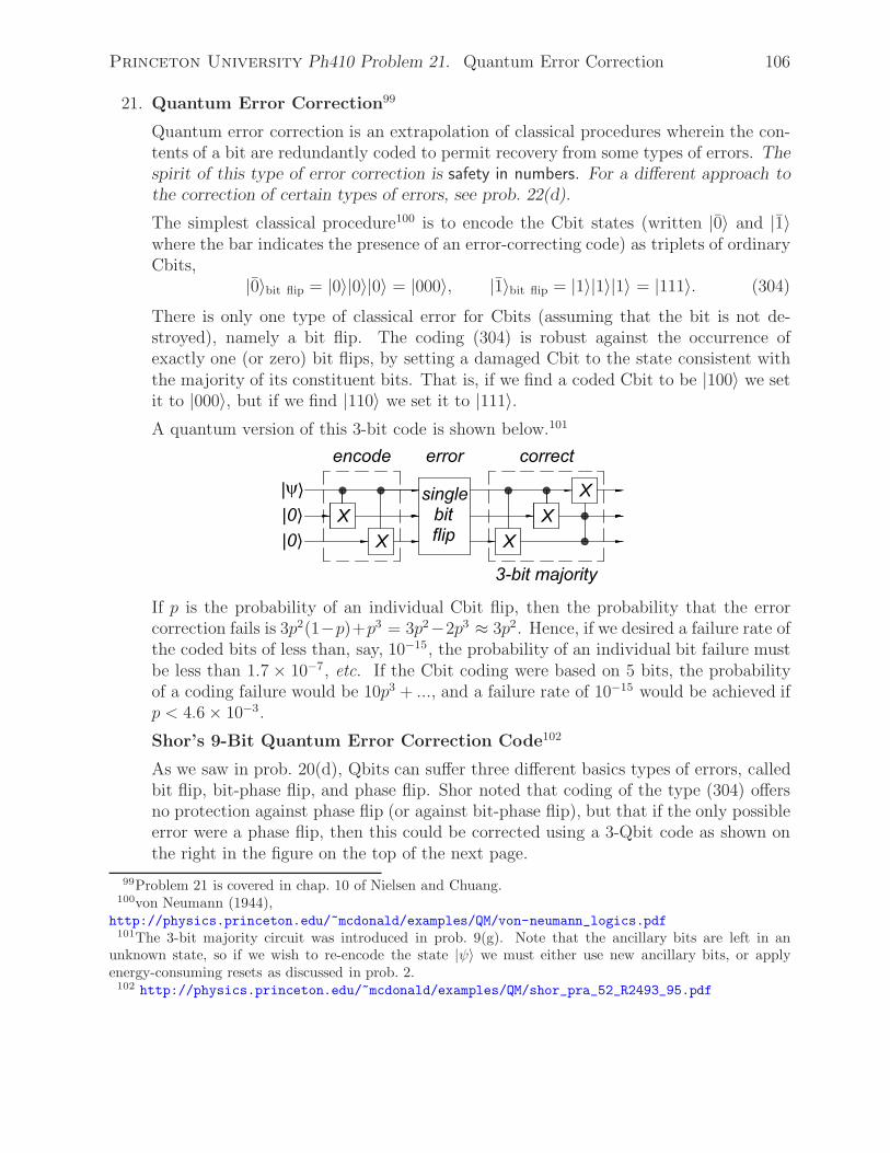
Princeton University Ph410 Problem 21. Quantum Error Correction 106
21. Quantum Error Correction99
Quantum error correction is an extrapolation of classical procedures wherein the con-tents of a bit are redundantly coded to permit recovery from some types of errors. Thespirit of this type of error correction is safety in numbers. For a different approach tothe correction of certain types of errors, see prob. 22(d).
The simplest classical procedure100 is to encode the Cbit states (written |0〉 and |1〉where the bar indicates the presence of an error-correcting code) as triplets of ordinaryCbits,
|0〉bit flip = |0〉|0〉|0〉 = |000〉, |1〉bit flip = |1〉|1〉|1〉 = |111〉. (304)
There is only one type of classical error for Cbits (assuming that the bit is not de-stroyed), namely a bit flip. The coding (304) is robust against the occurrence ofexactly one (or zero) bit flips, by setting a damaged Cbit to the state consistent withthe majority of its constituent bits. That is, if we find a coded Cbit to be |100〉 we setit to |000〉, but if we find |110〉 we set it to |111〉.A quantum version of this 3-bit code is shown below.101
If p is the probability of an individual Cbit flip, then the probability that the errorcorrection fails is 3p2(1−p)+p3 = 3p2−2p3 ≈ 3p2. Hence, if we desired a failure rate ofthe coded bits of less than, say, 10−15, the probability of an individual bit failure mustbe less than 1.7 × 10⁻⁷, etc. If the Cbit coding were based on 5 bits, the probabilityof a coding failure would be 10p3 + ..., and a failure rate of 10−15 would be achieved ifp < 4.6 × 10⁻³.
Shor’s 9-Bit Quantum Error Correction Code102
As we saw in prob. 20(d), Qbits can suffer three different basics types of errors, calledbit flip, bit-phase flip, and phase flip. Shor noted that coding of the type (304) offersno protection against phase flip (or against bit-phase flip), but that if the only possibleerror were a phase flip, then this could be corrected using a 3-Qbit code as shown onthe right in the figure on the top of the next page.
99Problem 21 is covered in chap. 10 of Nielsen and Chuang.100von Neumann (1944),
http://physics.princeton.edu/~mcdonald/examples/QM/von-neumann_logics.pdf101The 3-bit majority circuit was introduced in prob. 9(g). Note that the ancillary bits are left in an
unknown state, so if we wish to re-encode the state |ψ〉 we must either use new ancillary bits, or applyenergy-consuming resets as discussed in prob. 2.
102 http://physics.princeton.edu/~mcdonald/examples/QM/shor_pra_52_R2493_95.pdf

Princeton University Ph410 Problem 21. Quantum Error Correction 107
The coded basis states are
|0〉phase flip =|0〉 + |1〉√
2
|0〉 + |1〉√2
|0〉 + |1〉√2
= | + ++〉, (305)
|1〉phase flip =|0〉 − |1〉√
2
|0〉 − |1〉√2
|0〉 − |1〉√2
= | − −−〉. (306)
A phase-flip error turns the superposition |0〉 + |1〉 into |0〉 − |1〉, and vice versa. Shornoted that both of the logical Qbits (305)-(306) are eigenstates of the operators X1X2
and X2X3 with eigenvalue +1. If a phase-flip error had occurred on, say, the first bit ofeither |0〉phase flip or |1〉phase flip, then the “damaged” state is still an eigenstate of theoperators X1X2 and X2X3, but now the eigenvalues are −1 and +1, respectively. So ifwe apply these operators to the coded Qbits, those Qbits are not changed but we learnabout the presence of a phase-flip error from the pattern of the eigenvalues.
Shor then proposed “tripling” the phase-flip coding to the 9-bit forms
|0〉Shor =1
2√
2(|000〉 + |111〉)(|000〉 + |111〉)(|000〉 + |111〉), (307)
|1〉Shor =1
2√
2(|000〉 − |111〉)(|000〉 − |111〉)(|000〉 − |111〉), (308)
which provide protection against a single bit-flip or phase-flip error. Shor’s code couldbe realized by the circuit below.

Princeton University Ph410 Problem 21. Quantum Error Correction 108
We cannot, however, simply measure the state of Shor’s encoded Qbit (as a first step inthe error correction procedure) since this would destroy the superposition in eqs. (307)-(308), and in any case Shor’s states |0〉 and |1〉 cannot be distinguished by measure-ment.103
Shor’s suggestion is to measure the effect of various operators on the coded Qbit,
|ψ〉 = a|0〉 + b|1〉, (309)
where the operators are chosen such that states |0〉 and |1〉, as well as any state ob-tained from these via a single Qbit error, are eigenstates of the operators. (See alsoprob. 22(c).) Further, the eigenvalues should be the same for |0〉 and |1〉, and the samefor any pair of states obtained from these by a single Qbit error. Then, the codedstate |ψ〉 is unchanged, except for a possible overall phase, by the measurement. Ifthe results of the measurements permits us to deduce what kind of single-Qbit error,if any, has occurred, then that error can be corrected and the coded state restored toform (309) for any values of a and b.
As a first example, consider a single bit-flip error that occurs in the first triplet of the9-bit states. Then, the desired triplet combinations will be altered according to
|000〉± |111〉 → |100〉± |011〉, |010〉± |101〉, or |001〉± |110〉 (bit flip). (310)
Suitable operators to diagnose these errors are Z1Z2, Z2Z3 and Z1Z3, and it suffices toapply any two of them. Thus,
Z1Z2(|000〉 ± |111〉) = +(|000〉 ± |111〉), Z2Z3(|000〉 ± |111〉) = +(|000〉 ± |111〉),(311)Z1Z2(|100〉 ± |011〉) = −(|100〉 ± |011〉), Z2Z3(|100〉 ± |011〉) = +(|100〉 ± |011〉),(312)Z1Z2(|010〉 ± |101〉) = −(|010〉 ± |101〉), Z2Z3(|010〉 ± |101〉) = −(|010〉 ± |101〉),(313)Z1Z2(|001〉 ± |110〉) = +(|001〉 ± |110〉), Z2Z3(|001〉 ± |110〉) = −(|001〉 ± |110〉).(314)
The four possible sets of results of measurements of operators
Z1Z2 and Z2Z3 (315)
corresponds to the four possible error conditions in the first bit triplet: (+,+) impliesno error, (−,+) implies bit 1 was flipped, (−,−) implies bit 2 was flipped, and (+,−)implies bit 3 was flipped.
The error recovery procedure is to flip bits 1, 2 or 3 corresponding to the results (−,+),(−,−) or (+,−), respectively. Of, we do nothing when we obtain the result (+,+).
However, if two or three bits have been flipped in the first triplet of state (309), thepattern of eigenvalues of the operators (315) is:
Z1Z2(|110〉 ± |001〉) = +(|110〉 ± |001〉), Z2Z3(|110〉 ± |001〉) = −(|110〉 ± |001〉),(316)Z1Z2(|101〉 ± |010〉) = −(|101〉 ± |010〉), Z2Z3(|101〉 ± |010〉) = −(|101〉 ± |010〉),(317)Z1Z2(|011〉 ± |100〉) = −(|011〉 ± |100〉), Z2Z3(|011〉 ± |100〉) = +(|011〉 ± |100〉),(318)Z1Z2(|111〉 ± |000〉) = +(|111〉 ± |000〉), Z2Z3(|111〉 ± |000〉) = +(|111〉 ± |000〉).(319)
103Measurement is a key step in most quantum error-correction procedures. This is a kind of variant on thequantum Zeno effect whereby an unstable state can be kept from decaying if it is observed often enough.http://physics.princeton.edu/~mcdonald/examples/QM/misra_jmp_18_756_77 See also sec. 12.5 OfIntroduction to Quantum Mechanics, 2nd ed., by D.J. Griffiths (Prentice Hall, 2005).

Princeton University Ph410 Problem 21. Quantum Error Correction 109
Indeed, we see that the result (+,+) corresponds to either no error or to all 3 bitshaving flipped, while the result (+,−) occurs when either bit 3 has flipped or whenboth bits 1 and 2 have flipped, etc. If we apply the error-recovery procedure describedabove, then the results are |000〉 ± |111〉 → |111〉 ± |000〉 = ±(|000〉 ± |111〉), whichcould be described as a phase flip error in the coded bits |0〉 and |1〉.If the only type of Qbit errors were bit flips, a 3-Qbit code would suffice. As we willsee below, corrections of phase-flip errors requires use of more than 3 Qbits. In Shor’s9-bit code, (307)-(308), additional bit-flip errors can occur in the additional bits, butwe can use the two operators
Z4Z5 and Z5Z6, (320)
to detect a single error in the second bit triplet, and the two operators
Z7Z8 and Z8Z9, (321)
to spot a single error in the third triplet.
Turning to the issue of phase-flips errors, we see that the effect of such an error on anybit of a triplet state is
|000〉 ± |111〉 → |000〉 ∓ |111〉 (phase flip). (322)
To diagnose this error, we again seek operators for which both states |0〉 and |1〉 areeigenvectors with the same eigenvalue, and for which the damaged versions of thesestates are also eigenvectors with the same eigenvalue, but the eigenvalues are differentfor damaged and undamaged states.
Shor noted that the operator X1X2X3 plays the same role for his 9-Qbit code as theoperator X1 does for the 3-Qbit phase-flip code (305)-(306):
X1X2X3(|000〉 ± |111〉) = |111〉 ± |000〉 = ±(|000〉 ± |111〉). (323)
Operators for which the logical Qbits |0〉 and |1〉 are eigenstates with eigenvalue +1,and which also diagnose the presence of a single phase-flip error among the 9 physicalQbits, can be constructed out of six Xj ’s:
X1X2X3X4X5X6, X4X5X6X7X8X9, or X1X2X3X7X8X9. (324)
(a) Describe a procedure for diagnosis and correction of a single phase-flip error inShor’s coded Qbits (307)-(308).
(b) Verify that the procedures for diagnosis and correction of a single bit-flip errorand a single phase-flip error in Shor’s coded Qbits automatically correct a singlebit-phase-flip error as well. It suffices to consider a phase-flip error in the first ofthe nine Qbits of a coded Qbit.
(c) If px, py and pz are the probabilities of single-Qbit errors of types bit flip, bit-phaseflip, and phase flip, respectively, what are the leading probabilities of failure ofShor’s error-correcting scheme?

Princeton University Ph410 Problem 21. Quantum Error Correction 110
(d) We saw in prob. 20(d) that a general error on a single (physical) Qbit is describedby a set of operators {Ek} each of the form
Ek = a0I + a · σ = a0I + axX + ayY + azZ, (299)
where index k refers to a possible final state of the environment after its error-inducing interaction with the Qbit. Verify that the procedures for diagnosis andcorrection of a single bit-flip error and a single phase-flip error in Shor’s codedbits also correct for general single-bit errors. Again, it suffices to consider only anerror in the first of the nine Qbits of a coded Qbit.
Error Correction without Measurement?104
The process of error diagnosis and correction of a coded state |ψ〉 involves a set ofmeasurements, described by (hermitian) measurement operators {Mj}, and a corre-sponding set of unitary error-correction operators {Uj} that are applied conditionallyon the results of the measurements.
We can avoid the need to perform the measurements, which may be physically awk-ward, at the expense of introducing an additional n ancillary Qbits that must beinitially |0〉n at the time of each error-correction procedure.105
If there are m different measurement operators to be used, the number n of ancillaryQbits must be such that m < 2n, so that we can associate a different, nonzero basisstate of the ancillary Qbits to each measurement operator.
Then, we can create a new unitary operator U defined by
U|ψ〉|0〉n ≡ ∑j =0
(UjMj|ψ〉)|j〉n, (325)
U|ψ〉|k = 0〉n ≡ |ψ〉|k〉n. (326)
(e) Verify that the operator U is indeed unitary, i.e., it preserves inner products. Icould not actually verify this, and I worry that the claim is false.
The operation on the state |ψ〉|0〉n described by the first line of eq. (325) involves“virtual measurements” of all m types, followed by the corresponding error correction.Thus, the error is corrected without explicit measurements that force the state |ψ〉 intoone of its basis states.
However, at the end of the operation U, the ancillary Qbits are in an unknown, nonzerostate. If the error correction procedure is to be applied another time (or many timesas will be needed in general), we must either add new, initially zero, ancillary bits tothe system, or reset the ancillary Qbits. To reset these Qbits, we must either measurethem and apply the appropriate unitary reset operators, or we must invoke the energy-(and time-) consuming reset process of an unknown state that we considered in prob. 2.
104See Box 10.1, p. 439 of Nielsen and Chuang.105The 3-Qbit circuit shown at the beginning of this problem corrects single bit-flip errors without mea-
surement.

Princeton University Ph410 Problem 21. Quantum Error Correction 111
It appears that the use of quantum error correction will entail considerable costs: largenumbers of Qbits are required, as well as pauses in the calculation to make eithermeasurements or resets of ancillary Qbits. Or, if both measurements and resets are tobe avoided, a new set of ancillary Qbits is required at every error-correction cycle.
Error Correction Codes with Fewer Than Nine Qbits
Following Shor’s introduction of the 9-Qbit error correction code,106 it was quicklyrealized that quantum error-correction codes could be implemented with as few as 5physical Qbits per logical Qbit.107 Subsequent studies suggest that a 7-bit code may bethe best compromise between size and realizability.108 These codes are more complexthan Shor’s 9-Qbit code. For example, the logical Qbits of Steane’s 7-Qbit code are
|0〉Steane =1
2√
2(I + X4X5X6X7)(I + X2X3X6X7)(I + X1X3X5X7)|0000000〉
=1
2√
2(I + X1X3X5X7 + X2X3X6X7 + X4X5X6X7
+X1X2X5X6 + X1X3X4X6 + X2X3X4X5 + X1X2X4X7)
≡ 1
2√
2(I + M1 + M2 + M3 + M4 + M5 + M6 + M7)|0000000〉 ≡ 0Steane|0000000〉
=1
2√
2(|0000000〉 + |1010101〉 + |0110011〉 + |0001111〉+|1100110〉 + |1011010〉 + |0111100〉 + |1101001〉), (327)
|1〉Steane =1
2√
2(I + X4X5X6X7)(I + X2X3X6X7)(I + X1X3X5X7)|1111111〉
=1
2√
2(|1111111〉 + |0101010〉 + |1001100〉 + |1110000〉+|0011001〉 + |0100101〉 + |1000011〉 + |0010110〉) (328)
= X1X2X3X4X5X6X7|0〉Steane ≡ XSteane|0〉Steane = XSteane0Steane|0000000〉= 0Steane|1111111〉 = 0SteaneXSteane|0000000〉 ≡ 1Steane|0000000〉.
For the record, Steane’s error-correction procedure involves measurement of the sixoperators
X4X5X6X7, X2X3X6X7, X1X3X5X7, Z4Z5Z6Z7, Z2Z3Z6Z7, Z1Z3Z5Z7, (329)
for which both |0〉Steane and |1〉Steane are eigenvectors with eigenvalue +1 (while thestates resulting from a single Qbit error in |0〉Steane and |1〉Steane are eigenstates of theseoperators with eigenvalues ±1).109 If the measured eigenvalues of the first three oper-ators are all +1, then the pattern eigenvalues of the second three operators identifies
106 Shor’s code was independently developed by Steane,http://physics.princeton.edu/~mcdonald/examples/QM/steane_prl_77_793_96.pdf
107 http://physics.princeton.edu/~mcdonald/examples/QM/bennett_pra_54_3824_96.pdfhttp://physics.princeton.edu/~mcdonald/examples/QM/laflamme_prl_77_198_96.pdf
108 http://physics.princeton.edu/~mcdonald/examples/QM/calderbank_pra_54_1098_96.pdfhttp://physics.princeton.edu/~mcdonald/examples/QM/steane_prsl_a452_2551_96.pdf
109Indeed, |0〉Steane and |1〉Steane are eigenvectors with eigenvalue +1 of all seven operators Mj , as well asoperator 0Steane, introduced in eq. (327). Note also that all seven operators Mj commute with each other.

Princeton University Ph410 Problem 21. Quantum Error Correction 112
the presence of a bit-flip error. Similarly, if the measured eigenvalues of the secondthree operators are all +1, then the pattern eigenvalues of the first three operatorsidentifies the presence of a phase-flip error. And, if there are eigenvalues −1 amongthe measurements of both the first three and the second three operators, the patternof eigenvalues identifies the presence of a bit-phase-flip error.
We leave it to your discretion to verify these claims.
Error Codes That Can Recover from More Than One Error
In a recent paper, Crepeau et al. argue that approximate error correction codes can beconstructed in which a logical Qbit is encoded on n physical Qbits in such a mannerthat excellent recovery is possible from (n − 1)/2 errors.110 That is, an appropriate5-Qbit code can approximately correct for two errors, etc.
110 http://physics.princeton.edu/~mcdonald/examples/QM/crepeau_quant-ph-0503139.pdf

Princeton University Ph410 Problem 22. Fault-Tolerant Quantum Computation 113
22. Fault-Tolerant Quantum Computation111
The possibility of errors in quantum computation is by no means restricted to errors inthe Qbits themselves. Indeed, a more general type of error is the failure of a quantumoperation (gate) to perform as desired. Failures of gates can be more troublesomethan individual bit errors, since the action of a gate (such as the C-NOT) may be todistribute the information content of one bit among many others.
Fault-tolerant quantum computation follows the spirit of Qbit error correction introducedin prob. 21, which is to make multiple calculations of each quantum operation, andto take the majority result as the correct one. Typically, if the Qbit error-correctioncode involves n physical Qbits per logical Qbit, then n calculations of each quantumoperation will be made.
Again, we seek safety in numbers. For each logical gate in our basic circuit, we utilize≈ 20 physical gates in a fault-tolerant version of the circuit. Rules of thumb, optimisti-cally called threshold theorems, then suggest that there are about 104 places where anerror might occur in the fault-tolerant implementation of a quantum gate. So, if theprobability of a single error is less that 10−4, there will typically be 0 or 1 errors in theoperation of the gate, and the case of exactly 1 error will be properly corrected.
In prob. 12 we saw that any quantum computation can be built up from only 3 typesof gates, the Hadamard gate H, the Z1/4 gate, and the C-NOT gate. So, a sense ofthe methods of fault-tolerant quantum computation can be gained by demonstrationof fault-tolerant versions of each of these 3 gates, following the initial work by Shor.112
We will close with discussion of a recent suggestion by Grover for a different approachto fault-tolerant computation.
When we wish to implement a quantum operation U with logical Qbits |0〉 and |1〉, weneed to construct an operator U whose effect on the logical Qbits is the same as thatof operator U on physical Qbits. The details of the construction of U depend on thechoice of the error-correction code. The examples given here will be based on Steane’scode, eqs. (327)-(328), which has the merit that the constructions of many importantgates USteane are straightforward.
(a) Fault-Tolerant Hadamard Gate
If the logical version U of a single-Qbit operator U is obtained simply by applyingthe operator U to all n physical Qbits, we say that the logical gate U is transverse.
Not all single-Qbit operators USteane are transverse with respect to the Steanecoding of logical Qbits. It turns out that the Pauli gates XSteame (introducedin eq. (327) and ZSteane = Z1Z2Z3Z4Z4Z5Z6Z7, as well as the Hadamard gateHSteane = (XSteane + ZSteane)/
√2, are transverse for Steane’s code (327)-(328) (in
which the logical Qbit |0〉 contains an even number of |1〉’s while the logical Qbit
|1〉 contains an odd number). However, the gates YSteane and Z1/4Steane are not
transverse.
Here, we consider a transverse construction for the logical gate HSteane,
HSteane = H1H2H3H4H5H6H7. (330)
111Problem 22 is covered sec. 10.6 of Nielsen and Chuang.112 http://physics.princeton.edu/~mcdonald/examples/QM/shor_quant-ph-9605011.pdf
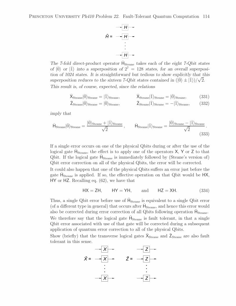
Princeton University Ph410 Problem 22. Fault-Tolerant Quantum Computation 114
The 7-fold direct-product operator HSteane takes each of the eight 7-Qbit statesof |0〉 or |1〉 into a superposition of 27 = 128 states, for an overall superposi-tion of 1024 states. It is straightforward but tedious to show explicitly that thissuperposition reduces to the sixteen 7-Qbit states contained in (|0〉 ± |1〉)/√2.
This result is, of course, expected, since the relations
XSteane|0〉Steane = |1〉Steane, XSteane|1〉Steane = |0〉Steane, (331)
ZSteane|0〉Steane = |0〉Steane, ZSteane|1〉Steane = −|1〉Steane, (332)
imply that
HSteane|0〉Steane =|0〉Steane + |1〉Steane√
2, HSteane|1〉Steane =
|0〉Steane − |1〉Steane√2
.
(333)
If a single error occurs on one of the physical Qbits during or after the use of thelogical gate HSteane, the effect is to apply one of the operators X, Y or Z to thatQbit. If the logical gate HSteane is immediately followed by (Steane’s version of)Qbit error correction on all of the physical Qbits, the error will be corrected.
It could also happen that one of the physical Qbits suffers an error just before thegate HSteane is applied. If so, the effective operation on that Qbit would be HX,HY or HZ. Recalling eq. (62), we have that
HX = ZH, HY = YH, and HZ = XH. (334)
Thus, a single Qbit error before use of HSteane is equivalent to a single Qbit error(of a different type in general) that occurs after HSteane, and hence this error wouldalso be corrected during error correction of all Qbits following operation HSteane.
We therefore say that the logical gate HSteane is fault tolerant, in that a singleQbit error associated with use of that gate will be corrected during a subsequentapplication of quantum error correction to all of the physical Qbits.
Show (briefly) that the transverse logical gates XSteane and ZSteane are also faulttolerant in this sense.

Princeton University Ph410 Problem 22. Fault-Tolerant Quantum Computation 115
(b) Fault-Tolerant C-NOT Gate
It is very agreeable that the logical operator C-NOTSteane = Cab, for use witha pair of Steane’s logical Qbits, |a〉 and |b〉, can be constructed transversely, asshown in the figure below.
Again, it is not self-evident that this construction works, but it is straightforwardto verify explicitly that the superpositions of 64 states in the output states |b〉from Cab reduce to the desired superpositions of only 8 states according to thetruth table for the C-NOT operator.
Give a (brief) analytic argument as to why the transverse construction of C-NOTSteane works, based on the operators 0Steane and 1Steane that were introducedin eqs. (327)-(328).
With the arguments of part (a) in mind, we readily see that the gate Cab is faulttolerant against a single Qbit error. The only difficult case is an error that occurson one of the physical Qbits of |a〉 before or during the C-NOT operation, becausesuch an error propagates to an error in the final state of |b〉 as well.
However, a single error in |a〉 leads to, at most, one error in each of |a〉 and |b〉.When we apply separate error-correction procedures to both the logical Qbits |a〉and |b〉 after the C-NOT operation, both of these errors are corrected.
Thus, the gate Cab is fault tolerant.
(c) Fault-Tolerant Z1/4 Gate
We first digress slightly to deduce the fractional powers p such that the gate Zp
could be implemented transversely with Steane’s 7-Qbit code. Recall that
Zp =
⎛⎝ 1 0
0 (−1)p
⎞⎠ =
⎛⎝ 1 0
0 eipπ
⎞⎠ . (335)
Hence, we must have
Zp|0〉 = |0〉, and Zp|1〉 = eipπ|1〉. (336)
It seems natural to seek a transverse construction of the form
ZpSteane = Zq1Zq2Z
q3Z
q4Z
q5Z
q6Z
q7, (337)
Princeton University Ph410 Problem 22. Fault-Tolerant Quantum Computation 116
for some power q. Since |0〉Steane is a superposition of states with either 0 or 4physical |1〉’s, while |1〉Steane is a superposition of states with either 3 or 7 physical|1〉’s, we must have
4q = 2m, so that Zp|0〉 = |0〉, (338)
3q = p+ 2n, so that Zp|1〉 = eipπ|1〉, (339)
for some integers m and n. Subtracting these, we find that q = 2(m−n)− p, andinserting this in either of eqs. (338) or (339) to eliminate q, we obtain
p =3m− 4n
2. (340)
Then, for (m,n) = (3, 2) we have p = 1/2, which is the only possible positivevalue of p less than one. In this case, q = 3/2, so we can make a transverseconstruction of the gate
Z1/2Steane = Z3/2
1 Z3/22 Z3/2
3 Z3/24 Z3/2
5 Z3/26 Z3/2
7 . (341)
However, we cannot construct the desired gate Z1/4Steane in a like manner.113 Instead,
we invoke a somewhat indirect approach, due to Boykin et al.114 They noted thatIF we can construct the state
|φ0〉 = Z1/4H|0〉 =|0〉 + eiπ/4|1〉√
2, (342)
that involves the operator Z1/4, and we combine it with a general Qbit |ψ〉 =a|0〉+ b|1〉 via a Controlled-NOT operation with |ψ〉 as the control Qbit and |φ0〉as the target Qbit,115 then we have
Cψφ0|ψ〉|φ0〉 = Cψφ0
(a|0〉 + b|1〉) |0〉 + eiπ/4|1〉√2
=a|0〉 + eiπ/4b|1〉√
2|0〉 +
eiπ/4a|0〉 + b|1〉√2
|1〉
= (Z1/4|ψ〉) |0〉√2
+ (Z−1/4|ψ〉)eiπ/4|1〉√
2. (343)
If we now measure the second Qbit (which originally was |φ0〉), we will either findit to be |0〉 (which forces the first Qbit into the state Z1/4|ψ〉), or |1〉 (which forcesthe first Qbit into the state Z−1/4|ψ〉 to within a phase).
113In principle, whenever we need to execute the logical operation Z1/4 on a logical Qbit |ψ〉 we couldconvert the coding from Steane’s version to another in which the Z1/4 can be constructed transversely, andthen convert back to Steane’s coding afterwards (A. McDonald, 4/28/05). However, I am not aware of anyerror coding in which a transverse construction of Z1/4 is possible. Since (eiπ/4)8 = 1, the coded state |0〉would have to involve 0 or 8 |1〉’s and |1〉 would have to involve 1 or 9 |1〉’s. So it seems that the code wouldneed to use at least 9 physical Qbits per logical Qbit.
114 http://physics.princeton.edu/~mcdonald/examples/QM/boykin_quant-ph-9906054.pdf115 Another version of this remarkable result is obtained if we use |φ0〉 as the control Qbit and |ψ〉 as the
target Qbit.

Princeton University Ph410 Problem 22. Fault-Tolerant Quantum Computation 117
We can bring the first Qbit to the state Z1/4|ψ〉 in both cases if we apply theoperator Z1/2 to the first Qbit conditional on the result of the measurement of thesecond Qbit being |1〉.This is a kind of quantum teleportation of the gate Z1/4 from the second Qbit tothe first Qbit!
In the above figure, the gate M represents a measurement of the second Qbit.
To successfully use this trick, we must augment it in two ways: we must create alogical state |φ0〉Steane that implements eq. (342) in the Steane code, and we mustfind a fault-tolerant version of the algorithm.
As the gate Z1/4Steane cannot be constructed transversely, we cannot create the logical
state |φ0〉Steane in an obvious manner. Boykin et al. noted that the desired state|φ0〉 is an eigenstate of the operator Uφ that can be represented two ways,
Uφ = Z1/4XZ−1/4 = e−iπ/4Z1/2X =
⎛⎝ 0 e−iπ/4
eiπ/4 0
⎞⎠ , (344)
the second form of which can be implemented in the Steane code with transverseoperators. The orthogonal eigenstate of Uφ is
|φ1〉 = Z1/4H|1〉 =|0〉 − eiπ/4|1〉√
2= Z|φ0〉, (345)
and we have Uφ|φj〉 = (−1)j |φj〉 for j = 0, 1.
Now that we have an operator Uφ whose eigenstates include the desired state|φ0〉, we can make a measurement of that operator, following a procedure due toShor,116 which will force the result into one of the eigenstates.
Show that the circuit show below (where |0〉 and |φ〉 are single physical Qbits)will take a general Qbit |φ〉 into the eigenstate |φ0〉 of operator Uφ, provided itstwo eigenvalues are ±1.
If, as holds in present case, the operator Uφ can be implemented transversely inSteane’s code, the state |φ〉 can be replaced by the 7-Qbit logical state |φ〉, andthe output of the measurement circuit will be the logical state |φ0〉. We can thenuse this state as the input to the Steane-code version of the previous circuit toobtain the gate Z
1/4Steane:
116 http://physics.princeton.edu/~mcdonald/examples/QM/shor_quant-ph-9605011.pdfShor’s measurement circuit was the prototype of the circuit of Boykin et al. shown at the top of the page.

Princeton University Ph410 Problem 22. Fault-Tolerant Quantum Computation 118
Finally, to make this procedure fault-tolerant, we apply Steane’s error correctionprocedure to the logical Qbits between every pair of logical gates.
Actually, it is more complicated than this to render the circuit fault tolerant.Extra effort must be made to protect the 7-fold measurement operator M fromerrors. In addition, we must also prepare the logical |0〉Steane states in a fault-tolerant manner. However, we leave to you pursue these details at a later time.
(d) Grover’s Fault-Tolerant Procedure117
Grover has recently proposed a procedure that addresses the possibility of a sys-tematic error in an operator U. Here, the purpose of operator U is to transform asource state |s〉 into a target state |t〉. That is, the desired operation is
U|s〉 = |t〉. (346)
However, due to defects in the construction of U, what actually happens is
U|s〉 = |t′〉 ≈ |t〉. (347)
If the operator U is reliable in the sense that it always produces the same output forthe same input, and we can also reliably construct the inverse operator U−1 = U †,then we can make an iterative use of these operators such that we come ever closerto the desired final state |t〉.To achieve this goal, Grover uses two additional operators that he calls Rs and Rt
whose effect on a general state
|ψ〉 = α|s〉 + β|u〉 = γ|t〉 + δ|v〉, (348)
where |u〉 is orthogonal to |s〉 and |v〉 is orthogonal to |t〉, is given by
Rs|ψ〉 = eiπ/3α|s〉 + β|u〉, and Rt|ψ〉 = eiπ/3γ|t〉 + δ|v〉. (349)
That is, operators Rs and Rt make selective phase shifts on the components |s〉and |t〉, respectively, of a general state.
Grover’s iteration operator is
V = URsU†Rt. (350)
Then, we claim, VU|s〉 is closer to the desired target state |t〉 than is U|s〉, andV2U|s〉 is closer still. In particular, if |〈t|U|s〉|2 = 1 − ε, then
∣∣∣〈t|URsU†RtU|s〉
∣∣∣2 = 1 − ε3, (351)
117 http://physics.princeton.edu/~mcdonald/examples/QM/grover_quant-ph-0503205.pdf

Princeton University Ph410 Problem 22. Fault-Tolerant Quantum Computation 119
and even one iteration greatly reduces the error in the calculation of the targetstate.
Show that
URsU†RtU|s〉 = [eiπ/3 + |〈t|U|s〉|2 (eiπ/3 − 1)2]U|s〉 + 〈t|U|s〉(eiπ/3 − 1)|t〉, (352)
As a measure of the deviation of this state from the target state |t〉, calculatethe square of the amplitude of the part of eq. (352) that is orthogonal to |t〉,i.e., calculate that probability that the result of the first iteration is not state |t〉.Show that this probability is
(1 − |〈t|U|s〉|2)∣∣∣eiπ/3 + |〈t|U|s〉|2 (eiπ/3 − 1)2
∣∣∣2 = ε3, (353)
if |〈t|U|s〉|2 = 1 − ε.
Grover notes that this procedure is a kind of quantum search algorithm duringwhich one monotonically converges on the goal, in contrast to the search algorithmof prob. 15, in which one is close to the goal only at various stages of a quasi-cyclicprocess. This may help dispel the perception that quantum computation is moreof an art than a science, as has been quipped: “The quantum search algorithm islike baking a souffle....you have to stop at just the right time or it gets burnt.”118
118 http://physics.princeton.edu/~mcdonald/examples/QM/brassard_science_275_627_97.pdf
Princeton University Ph410 Problem 23. Quantum Cryptography 120
23. Quantum Cryptography119
We have already discussed one aspect of quantum cryptography in problem 17, namely,how quantum computation might be used to decode so-called public keys based on largeprime numbers. Here, we explore how quantum techniques might improve the securityof private keys based on one-time pads.
The goal is the transmission of “secret” messages, which for computational purposesare taken to be strings of bits. A message is encoded (and subsequently decoded) byadding (modulo 2) each bit of the message to a corresponding bit from a private key.For maximal security, the key should consist of a random bit string of same lengthas the message, and the key should be used for one time only (Vernam, 1917). Thedifficulty with this scheme is that the key must be shared between the sender andreceiver via a communication channel that is subject to “eavesdropping”, i.e., a publicchannel.
The challenge is to devise a procedure to generate a (random) private key that can besent over a public channel.
As classical bit strings can be copied exactly (without altering the originals), the trans-mission of classical private keys over public channels is unsatisfactory. However, theno-cloning theorem (prob. 6) suggests that quantum cryptography may offer advan-tages, since an unknown quantum state cannot in general be copied exactly (and mea-surements of a large number of copies of an unknown quantum state are required todetermine its character to good accuracy).
(a) Demonstrate the following variant on the no-cloning theorem. Suppose that Eveintercepts a quantum state |ψ〉 from, say, a public communication channel, andshe wishes to determine if this state is distinct from another state |φ〉. Show thatthis cannot be done, in general, without modification to state |ψ〉.Hint: You may suppose that Eve tries to distinguish |ψ〉 from |φ〉 with the aid ofan ancillary state |a〉 and a unitary transformation U such that
U|ψ〉|a〉 = |ψ〉|b〉, and U|φ〉|a〉 = |φ〉|c〉, (354)
which leaves states |ψ〉 and |φ〉 unaltered. Show, however, that if 〈ψ|φ〉 = 0, then〈b|c〉 = 1 and thus |ψ〉 and |φ〉 cannot be distinguished by this procedure (unless|ψ〉 and |φ〉 are orthogonal).
Problem (a) alerts us to another difficulty in cryptography that uses a public channel,namely that messages and keys may be altered by an eavesdropper, or by Naturevia various forms of bit errors. To guard against the latter issue, we anticipate thatpractical quantum cryptography would be performed with logical Qbits based on error-correction codes (prob. 21). If the tampering of an n-bit key by an eavesdropper isknown to be limited to at most m < n bits, then a largely classical procedure calledprivacy amplification can be used to build a relatively secure key of length < n − mbits.120 Here, we turn directly to schemes for secure transmission of a private key overa public channel.
119See sec. 12.6 of Nielsen and Chuang.120 http://physics.princeton.edu/~mcdonald/examples/QM/bennett_siamjc_17_210_88.pdf

Princeton University Ph410 Problem 23. Quantum Cryptography 121
The BB84 Scheme for Generation of a Private Key Using a Public Chan-nel.121
i. Alice encodes an n-bit string in n Qbits where the basis of each Qbit is chosenat random among the [0,1] and [+,−] bases. In practice, these Qbits could bephotons in an optical fiber, where the [0,1] basis corresponds to horizontal andvertical linear polarization, and the [+,−] basis corresponds to 45◦ and 135◦
linear polarization; alternatively, the second basis could be left- and right-handedcircular polarization related by |L,R〉 = (|x〉 ± i|y〉)/√2.
ii. Alice sends the n Qbits to Bob over a public communication channel. For now,we ignore the possibility of bit errors and/or tampering by an eavesdropper.
iii. Bob measures each of the Qbits in either the [0,1] or the [+,−] basis, choosingthe basis at random for each bit.
iv. Alice announces over the public channel in which basis she created each of thebits (but she does not announce the values of the bits).
v. Likewise, Bob announces over the public channel which basis he used to measureeach of the bits (but he does not announce the results of the measurements)
vi. Alice and Bob now share a private key, of length roughly n/2 bits, consisting ofthose bits for which they used the same basis for creation/measurement.
(b) An eavesdropper Eve wishes to gain as much information as possible about theprivate key of Alice and Bob, so she performs a “nondemolition” measurementon each of the transmitted Qbits, as discussed in prob. 5(d). How much of thekey can Eve learn, and what effect do her actions have on the key? For yourown satisfaction, you may want to verify that the results would be the same ifEve destructively measures each Qbit, and then sends on to Bob a new Qbit ofwhatever value she measured.
The no-cloning theorem advises us that Eve cannot learn all details as to the privatekey of Alice and Bob. From prob. (a) we anticipate that Eve’s gain in knowledgecomes at the expense of alterations to the bits received by Bob. Thus, while Alice andBob can be confident that their private key cannot be completely broken by Eve, theycannot be sure, without further checking, that their own versions of the private keyare actually the same. However, as you have deduced in prob. (b), there is a boundon how much damage Eve does to the private key if she only tries to learn its details.Alice and Bob could verify the extent of the damage by publicly comparing/sacrificingsome fraction of the bits of their not-quite-private key, and then use the technique ofprivacy amplification to generate a shorter, but more truly private key.
The E91 Variant122
Among the many variants proposed for quantum key distribution, one of the moreinteresting concepts is that due to Ekert, in which the key is derived from pairs ofentangled bits generated by Alice (or by Bob or even by a third party) such that
121 http://physics.princeton.edu/~mcdonald/examples/QM/bennett_ieeecssp_175_84.pdf122 http://physics.princeton.edu/~mcdonald/examples/QM/ekert_prl_67_661_91.pdf
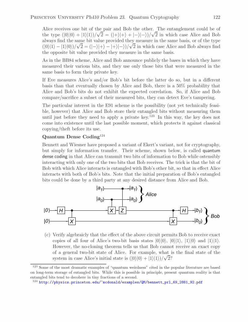
Princeton University Ph410 Problem 23. Quantum Cryptography 122
Alice receives one bit of the pair and Bob the other. The entanglement could be ofthe type (|0〉|0〉 + |1〉|1〉)/√2 = (|+〉|+〉 + |−〉|−〉)/√2 in which case Alice and Bobalways find the same bit value provided they measure in the same basis, or of the type(|0〉|1〉 − |1〉|0〉)/√2 = (|−〉|+〉 − |+〉|−〉)/√2 in which case Alice and Bob always findthe opposite bit value provided they measure in the same basis.
As in the BB84 scheme, Alice and Bob announce publicly the bases in which they havemeasured their various bits, and they use only those bits that were measured in thesame basis to form their private key.
If Eve measures Alice’s and/or Bob’s bit before the latter do so, but in a differentbasis than that eventually chosen by Alice and Bob, there is a 50% probability thatAlice and Bob’s bits do not exhibit the expected correlation. So, if Alice and Bobcompare/sacrifice a subset of their measured bits, they can detect Eve’s tampering.
The particular interest in the E91 scheme is the possibility (not yet technically feasi-ble, however) that Alice and Bob store their entangled bits without measuring themuntil just before they need to apply a private key.123 In this way, the key does notcome into existence until the last possible moment, which protects it against classicalcopying/theft before its use.
Quantum Dense Coding124
Bennett and Wiesner have proposed a variant of Ekert’s variant, not for cryptography,but simply for information transfer. Their scheme, shown below, is called quantumdense coding in that Alice can transmit two bits of information to Bob while ostensiblyinteracting with only one of the two bits that Bob receives. The trick is that the bit ofBob with which Alice interacts is entangled with Bob’s other bit, so that in effect Aliceinteracts with both of Bob’s bits. Note that the initial preparation of Bob’s entangledbits could be done by a third party at any desired distance from Alice and Bob.
(c) Verify algebraicly that the effect of the above circuit permits Bob to receive exactcopies of all four of Alice’s two-bit basis states |0〉|0〉, |0〉|1〉, |1〉|0〉 and |1〉|1〉.However, the no-cloning theorem tells us that Bob cannot receive an exact copyof a general two-bit state of Alice. For example, what is the final state of thesystem in case Alice’s initial state is (|0〉|0〉 + |1〉|1〉)/√2?
123 Some of the most dramatic examples of “quantum weirdness” cited in the popular literature are basedon long-term storage of entangled bits. While this is possible in principle, present quantum reality is thatentangled bits tend to decohere in tiny fractions of a second.
124 http://physics.princeton.edu/~mcdonald/examples/QM/bennett_prl_69_2881_92.pdf
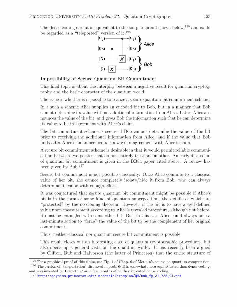
Princeton University Ph410 Problem 23. Quantum Cryptography 123
The dense coding circuit is equivalent to the simpler circuit shown below,125 and couldbe regarded as a “teleported” version of it.126
Impossibility of Secure Quantum Bit Commitment
This final topic is about the interplay between a negative result for quantum cryptog-raphy and the basic character of the quantum world.
The issue is whether is it possible to realize a secure quantum bit commitment scheme.
In a such a scheme Alice supplies an encoded bit to Bob, but in a manner that Bobcannot determine its value without additional information from Alice. Later, Alice an-nounces the value of the bit, and gives Bob the information such that he can determineits value to be in agreement with Alice’s claim.
The bit commitment scheme is secure if Bob cannot determine the value of the bitprior to receiving the additional information from Alice, and if the value that Bobfinds after Alice’s announcements is always in agreement with Alice’s claim.
A secure bit commitment scheme is desirable in that it would permit reliable communi-cation between two parties that do not entirely trust one another. An early discussionof quantum bit commitment is given in the BB84 paper cited above. A review hasbeen given by Bub.127
Secure bit commitment is not possible classically. Once Alice commits to a classicalvalue of her bit, she cannot completely isolate/hide it from Bob, who can alwaysdetermine its value with enough effort.
It was conjectured that secure quantum bit commitment might be possible if Alice’sbit is in the form of some kind of quantum superposition, the details of which are“protected” by the no-cloning theorem. However, if the bit is to have a well-definedvalue upon measurement according to Alice’s revealed procedure, although not before,it must be entangled with some other bit. But, in this case Alice could always take alast-minute action to “force” the value of the bit to be the complement of her originalcommitment.
Thus, neither classical nor quantum secure bit commitment is possible.
This result closes out an interesting class of quantum cryptographic procedures, butalso opens up a general vista on the quantum world. It has recently been arguedby Clifton, Bub and Halvorson (the latter of Princeton) that the entire structure of
125 For a graphical proof of this claim, see Fig. 1 of Chap. 6 of Mermin’s course on quantum computation.126 The version of “teleportation” discussed in prob. 6(d) is somewhat more sophisticated than dense coding,
and was invented by Bennett et al. a few months after they invented dense coding.127 http://physics.princeton.edu/~mcdonald/examples/QM/bub_fp_31_735_01.pdf

Princeton University Ph410 Problem 23. Quantum Cryptography 124
quantum theory can be deduced from three negative-sounding information-theoreticconstraints:128
• No superluminal information transfer.
• No broadcasting/cloning of an unknown (quantum) state.
• No secure bit commitment.
Of these three constraints, the first and the third hold in the classical as well asthe quantum world. Hence, it appears that the no-cloning theorem represents theessential distinction between the classical and the quantum worlds (beyond such detailsas classical bits having values of only 0 or 1, while quantum bits can be a superpositionof |0〉 and |1〉 with imaginary coefficients).
128 http://physics.princeton.edu/~mcdonald/examples/QM/clifton_quant-ph-0211089.pdf

Princeton University Ph410 Problem 24. The End of Quantum Information? 125
24. The End of Quantum Information?
In prob. 1 we referred briefly to the possibility of very compact quantum computers – ofthe size of a 1-kg black hole. Here we return to the theme of black holes and quantuminformation, and comment on unresolved issues of potentially deep significance.
In 1974 Stephen Hawking had the important insight that the interaction of (classical)black holes with quantum fluctuations of the “vacuum” leads to “evaporation” of theblack holes.129 Hawking argued that the radiation from the evaporating black hole hasa purely thermal spectrum, with temperature T related to the acceleration g of gravityat the Schwarzschild radius of the black hole by kT = hg/2π, where k is Boltzmann’sconstant.
The existence of Hawking radiation makes a dramatic change in the character of anolder paradox concerning black holes. If a black hole “swallows” a collection of par-ticles with entropy S, that entropy is no longer accessible to the Universe exterior tothe black hole.130 Hence, it might seem that black holes violate the second law ofthermodynamics. However, if the black hole is a stable object, one can say that itstores the entropy that it “swallowed”, so that the total entropy of the Universe hasnot really decreased (although some of the entropy is not very accessible), and there isnot actually a paradox.
But if/when the black hole evaporates, what has become of the entropy that was storedinside it? If the radiation that leads to the disappearance of the black hole is indeedthermal as Hawking claimed, this radiation cannot carry the information correspondingto the stored entropy. When the black hole has completely evaporated, the entropy ofthe Universe has decreased, and the paradox is severe.
The resolution of this paradox has been a major issue for theoretical physics over thepast 30 years. Various solutions have been suggested, including131
• The second law of thermodynamics is indeed violated by black holes, so that newlaws of physics are required to resolve the paradox.
• Black holes don’t evaporate completely, but “remnants” continue to store the“swallowed” entropy (perhaps in a “baby” universe).
• Hawking radiation is not thermal, such that entropy “leaks” back out of the blackhole all the time.
129 http://physics.princeton.edu/~mcdonald/examples/QED/hawking_nature_248_30_74.pdfhttp://physics.princeton.edu/~mcdonald/examples/QED/hawking_cmp_43_199_75.pdfA rough model is that the gravitational potential energy of a black hole is converts electron-positron pairs inthe QED vacuum (just outside the Schwarzschild radius of the black hole) from “virtual” to real particles,which then annihilate in to pair of real photons one of which is captured by the black hole and the other ofwhich is radiated to “infinity”.
130The entropy kA/L2P (mentioned in prob. 1) that is associated with the surface area A of a black hole is
much less, in general, than the amount of entropy that the black hole can have “swallowed”.131For a review of the situation in 1992 from an information theoretic perspective, see
http://physics.princeton.edu/~mcdonald/examples/QM/preskill_hep-th-9209058.pdfHawking’s recent views appear inhttp://physics.princeton.edu/~mcdonald/examples/QM/hawking_prd_72_084013_05.pdf
Princeton University Ph410 Problem 24. The End of Quantum Information? 126
• Black holes do evaporate, but somehow the entropy comes out in a burst at theend.132
• Black holes do evaporate, and the entropy “leaks” out continuously into a quan-tum state surrounding the black hole, such that this entropy/information is inac-cessible until a quantum key is released by the black hole at the very end of itslife.133
The last two conjectures are in the spirit of John Wheeler’s notion of “It from Bit.”Your assignment (with no time limit) is to clarify and extend these ideas to help bringabout a more unified understanding of our quantum Universe.134
132 http://physics.princeton.edu/~mcdonald/examples/QM/carlitz_prd_36_2336_87.pdfhttp://physics.princeton.edu/~mcdonald/examples/QM/horowitz_jhep_022004008.pdfhttp://physics.princeton.edu/~mcdonald/examples/QM/gottesman_hep-ph-0311269.pdf
133 http://physics.princeton.edu/~mcdonald/examples/QM/smolin_prl_96_081302_06.pdf134A sketch of a partial answer by Preskill is given at
http://www.theory.caltech.edu/people/preskill/talks/GR100-Caltech-preskill.pdf.
Princeton University Ph410 Solution 1. The Ultimate Laptop 127
1. The Ultimate Laptop
Energy Limits Speed
The time interval Δt during which a quantum process takes place is bounded by theenergy scale E associated with that process by the uncertainty principle,
Δt ≥ h
E. (355)
So if the laptop has energy E available for computation, the number N of processingcycles per second is limited by
N ≈ 1
Δt≤ E
h. (356)
In our ultimate laptop, we suppose that all of the rest energy is available to drive thecomputation. Then, according to Einstein,
E = mlaptopc2 = 1 · (3 × 108)2 ≈ 1017 J, (357)
and the speed of the laptop is
N ≈ E
h≈ 1017 J
10−34 J-s≈ 1051 bit operations/s. (358)
However, for the full rest energy to be available, the laptop must be hot enough thatthe nucleons are unbound, and can be transformed into other forms of mass/energy.That is, the temperature must be related to the mass of a proton mp by
kT ≈ mpc2, or T ≈ mpc
2
k≈ 10−27(3 × 10⁸)2
10−23≈ 1013K. (359)
For additional discussion, see, for examplehttp://physics.princeton.edu/~mcdonald/examples/QM/margolis_physica_d120_188_98.pdf
Transit Time
The above argument ignores possible restrictions due to signal propagation from onepart of the laptop to the other.
In 1 kg there are about 1027 nucleons. If there are 1051 operations per second in total,then each nucleon must perform about 1024 operations per second. Once the laptophas been converted to a plasma with temperature T ≈ 1013K, the average distancebetween nucleons is about 1 Angstrom = 10−10 m. It takes light about 3 × 10⁻¹⁹ s totravel this distance, so each nucleon could communicate with its nearest neighbor onlyabout 3 × 10¹⁸ times per second. Such communication is necessary for computation,so we should derate the ultimate laptop from 1051 operations per second to about 1045
operations per second.
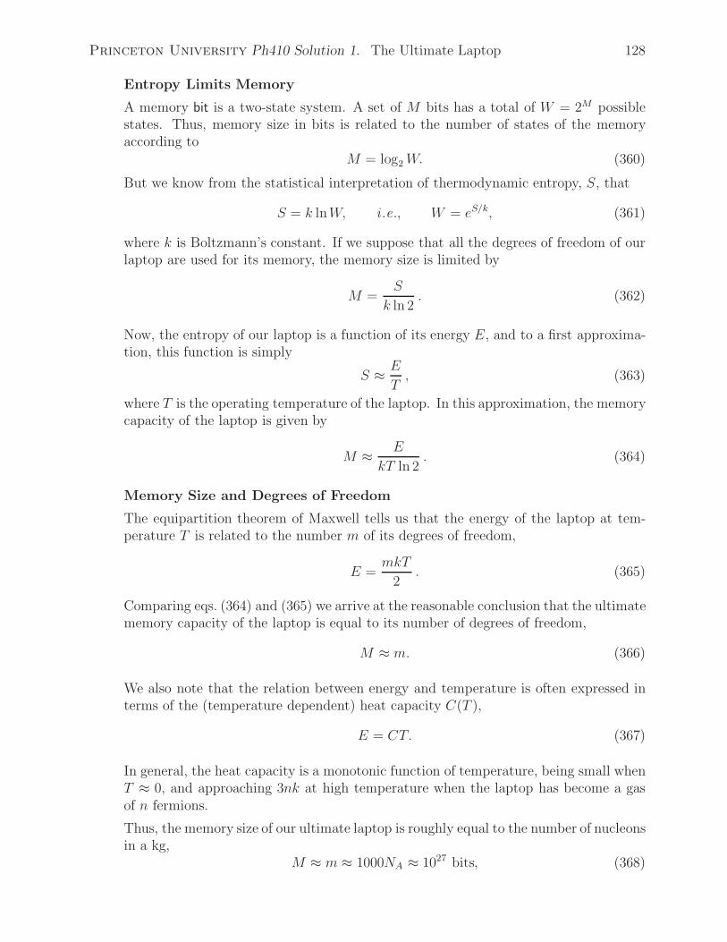
Princeton University Ph410 Solution 1. The Ultimate Laptop 128
Entropy Limits Memory
A memory bit is a two-state system. A set of M bits has a total of W = 2M possiblestates. Thus, memory size in bits is related to the number of states of the memoryaccording to
M = log2W. (360)
But we know from the statistical interpretation of thermodynamic entropy, S, that
S = k lnW, i .e., W = eS/k, (361)
where k is Boltzmann’s constant. If we suppose that all the degrees of freedom of ourlaptop are used for its memory, the memory size is limited by
M =S
k ln 2. (362)
Now, the entropy of our laptop is a function of its energy E, and to a first approxima-tion, this function is simply
S ≈ E
T, (363)
where T is the operating temperature of the laptop. In this approximation, the memorycapacity of the laptop is given by
M ≈ E
kT ln 2. (364)
Memory Size and Degrees of Freedom
The equipartition theorem of Maxwell tells us that the energy of the laptop at tem-perature T is related to the number m of its degrees of freedom,
E =mkT
2. (365)
Comparing eqs. (364) and (365) we arrive at the reasonable conclusion that the ultimatememory capacity of the laptop is equal to its number of degrees of freedom,
M ≈ m. (366)
We also note that the relation between energy and temperature is often expressed interms of the (temperature dependent) heat capacity C(T ),
E = CT. (367)
In general, the heat capacity is a monotonic function of temperature, being small whenT ≈ 0, and approaching 3nk at high temperature when the laptop has become a gasof n fermions.
Thus, the memory size of our ultimate laptop is roughly equal to the number of nucleonsin a kg,
M ≈ m ≈ 1000NA ≈ 1027 bits, (368)

Princeton University Ph410 Solution 1. The Ultimate Laptop 129
where NA is Avagadro’s number. This result could have been anticipated without thedigression about entropy.
Ultimate Speed of a Room-Temperature Laptop
Backing away from a laptop whose state of matter is something like that in the earlyuniverse, we return to room temperature. Then, the ultimate memory size is still givenby eq. (368). To estimate the speed according to eq. (356), we note that the availableenergy is roughly
Eroom temp ≈ mkT ≈ 1027 · (1/40) eV ≈ 1027 · 1
40· 10−19 J ≈ 106 J. (369)
The ultimate bit-operation speed of a room-temperature laptop is therefore
Nroom temp ≈ Eroom temp
h≈ 106
10−34≈ 1040/s, (370)
which evades our most optimistic transit-time limit.
The Black-Hole Laptop
Bekenstein’s result that inspired this problem is that the entropy of a black hole is
S ≈ kA
L2P
≈ kR2S
L2P
, (371)
where the Schwarzschild radius of an object of mass m is
RS =2Gm
c2, (372)
and the Planck length is
LP =
√Gh
c3. (373)
Combining these with eq. (362), the memory size M of a black hole is
M ≈ R2S
L2P
=Gm2
hc. (374)
The memory size of a 1-kg black-hole laptop is
Mblack−hole laptop ≈ 10−10 · 12
10−34 · 108≈ 1016 bits. (375)
While still quite large, this is a substantial reduction compared to the ultimate memorycapacity (368) of a laptop of ordinary density.
See also,http://physics.princeton.edu/~mcdonald/examples/QM/gambini_quant-ph-0507262.pdf
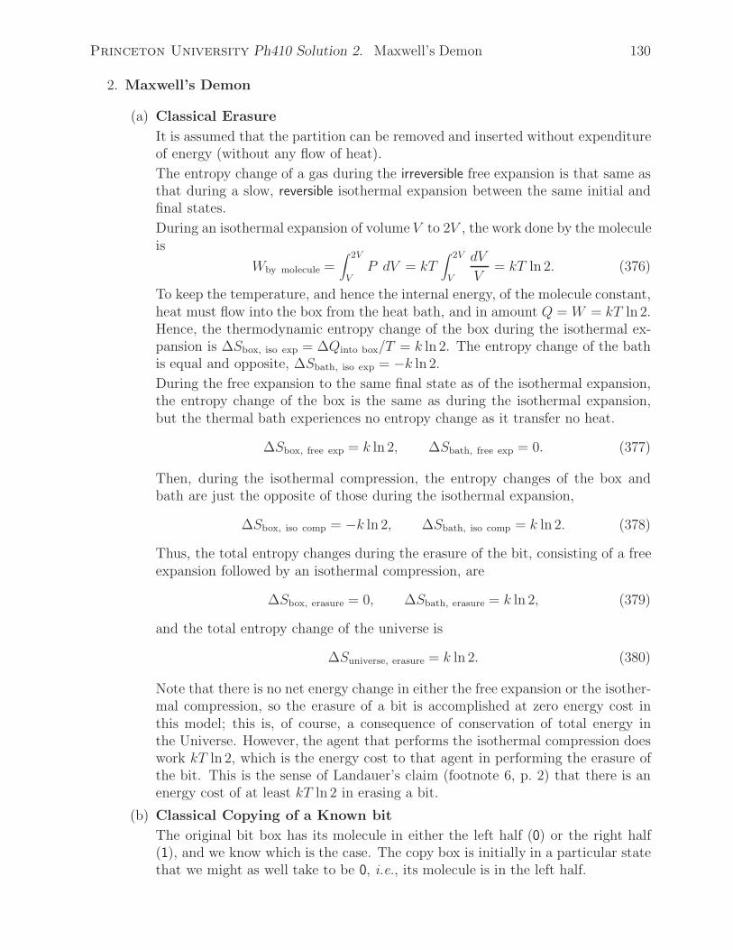
Princeton University Ph410 Solution 2. Maxwell’s Demon 130
2. Maxwell’s Demon
(a) Classical Erasure
It is assumed that the partition can be removed and inserted without expenditureof energy (without any flow of heat).
The entropy change of a gas during the irreversible free expansion is that same asthat during a slow, reversible isothermal expansion between the same initial andfinal states.
During an isothermal expansion of volume V to 2V , the work done by the moleculeis
Wby molecule =∫ 2V
VP dV = kT
∫ 2V
V
dV
V= kT ln 2. (376)
To keep the temperature, and hence the internal energy, of the molecule constant,heat must flow into the box from the heat bath, and in amount Q = W = kT ln 2.Hence, the thermodynamic entropy change of the box during the isothermal ex-pansion is ΔSbox, iso exp = ΔQinto box/T = k ln 2. The entropy change of the bathis equal and opposite, ΔSbath, iso exp = −k ln 2.
During the free expansion to the same final state as of the isothermal expansion,the entropy change of the box is the same as during the isothermal expansion,but the thermal bath experiences no entropy change as it transfer no heat.
ΔSbox, free exp = k ln 2, ΔSbath, free exp = 0. (377)
Then, during the isothermal compression, the entropy changes of the box andbath are just the opposite of those during the isothermal expansion,
ΔSbox, iso comp = −k ln 2, ΔSbath, iso comp = k ln 2. (378)
Thus, the total entropy changes during the erasure of the bit, consisting of a freeexpansion followed by an isothermal compression, are
ΔSbox, erasure = 0, ΔSbath, erasure = k ln 2, (379)
and the total entropy change of the universe is
ΔSuniverse, erasure = k ln 2. (380)
Note that there is no net energy change in either the free expansion or the isother-mal compression, so the erasure of a bit is accomplished at zero energy cost inthis model; this is, of course, a consequence of conservation of total energy inthe Universe. However, the agent that performs the isothermal compression doeswork kT ln 2, which is the energy cost to that agent in performing the erasure ofthe bit. This is the sense of Landauer’s claim (footnote 6, p. 2) that there is anenergy cost of at least kT ln 2 in erasing a bit.
(b) Classical Copying of a Known bit
The original bit box has its molecule in either the left half (0) or the right half(1), and we know which is the case. The copy box is initially in a particular statethat we might as well take to be 0, i.e., its molecule is in the left half.

Princeton University Ph410 Solution 2. Maxwell’s Demon 131
The copying can be accomplished as follows:135
i. If the original bit is 0, do nothing to the copy bit, which already was 0.
ii. If the original bit is 1, rotate the copy box by 180◦ about an axis in its left-right midplane. After this, the molecule appears to be in the right half of thecopy box, and is therefore in a 1 state as desired.
No energy is expended in any of these steps. No heat flows. Hence, there is no(thermodynamic) entropy change in either the computer or in the environment.
The rotation of the copy box by 180◦ is equivalent to the logical NOT operation.Thus, the copying procedure suggested above could be called a controlled-NOToperation, in which the NOT operation is performed only if a relevant controlbit is in the 1 state. Since all computation involves changing 0’s into 1’s andvice versa, we get a preview of the important role of controlled-NOT operations inclassical and quantum computation.
The trick of rotating a box by 180◦ if it is in a 1-state to bring it to the 0-stateis a possible process for classical erasure of a bit. However, this process requiresknowledge of the initial state of the box, whereas the method or part (a) does notrequire such knowledge. So, rotation of the box is not a solution to part (a) asposed.
Since the rotation of the box is a reversible process, it doesn’t change entropy.Could it then be that the trick of rotating the box provides a means of erasurewith no entropy cost?
The issue now whether the task of acquiring the knowledge as to the state of theboth implies an increase of entropy, of at least k ln 2.
This is a famous question, associated with the concept of negentropy – that in-formation is associated with a kind of negative entropy, and that the creation ofinformation implies a corresponding increase of entropy somewhere in the largersystem.
A sense of this was noted already in 1868 by P.T. Tait, Sketch of Thermodynamics,p. 100.136 A longer discussion was given by Brilloun.137
If the box has moment of inertia I and we wish to accomplish the erasure in time t, we givethe box constant angular acceleration θ = 4π/t2 for time t/2 and then the negative of thisfor an additional time t/2 to leave the box at rest after rotation by π radians. The torquerequired during this process is τ = Iθ = 4πI/t2, so the work done in rotating the box isW = τΔθ = πτ = 4π2I/t2.
For a box that consists of a pair of C60 “buckyballs,” of mass m = 60mC ≈ 720mp and radiusr ≈ 0.5 nm each, the moment of inertia is I ≈ 2mr2(1 + 2/3) = 10mr2/3 ≈ 6 × 10⁻¹⁶mp ≈10−42 J. If the erasure to be accomplished in time t = 0.1 ns (10 GHz), the work done in rotatingthe box is W = 4π2I/t2 ≈ 4 × 10⁻²¹ J ≈ 1/40 eV = kT for room temperature.
That is, even the rotating pair of buckyballs as a memory element obeys Landauer’s claim that
the energy cost of erasure is at least kT ln 2 for “practical” parameters.
135A scheme involving two pistons and the (re)movable partition, but no rotation, also works.136 http://physics.princeton.edu/~mcdonald/examples/statmech/tait_thermo_68_p100.txt137L. Brillouin, The Negentropy Principle of Information, J. Appl. Phys. 24, 1152 (1953),
http://physics.princeton.edu/~mcdonald/examples/statmech/brillouin_jap_24_1152_53
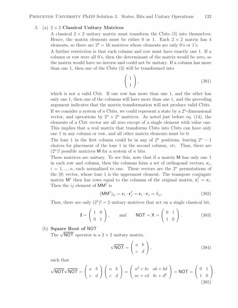
Princeton University Ph410 Solution 3. States, Bits and Unitary Operations 132
3. (a) 2 × 2 Classical Unitary Matrices
A classical 2 × 2 unitary matrix must transform the Cbits (3) into themselves.Hence, the matrix elements must be either 0 or 1. Each 2 × 2 matrix has 4elements, so there are 24 = 16 matrices whose elements are only 0’s or 1’s.
A further restriction is that each column and row must have exactly one 1. If acolumn or row were all 0’s, then the determinant of the matrix would be zero, sothe matrix would have no inverse and could not be unitary. If a column has morethan one 1, then one of the Cbits (3) will be transformed into⎛
⎝ 1
1
⎞⎠ , (381)
which is not a valid Cbit. If one row has more than one 1, and the other hasonly one 1, then one of the columns will have more than one 1, and the precedingargument indicates that the matrix transformation will not produce valid Cbits.
If we consider a system of n Cbits, we could represent a state by a 2n-dimensionalvector, and operations by 2n × 2n matrices. As noted just before eq. (14), theelements of a Cbit vector are all zero except of a single element with value one.This implies that a real matrix that transforms Cbits into Cbits can have onlyone 1 in any column or row, and all other matrix elements must be 0.
The lone 1 in the first column could be in any of 2n positions, leaving 2n − 1choices for placement of the lone 1 in the second column, etc. Thus, there are(2n)! possible matrices M for a system of n bits.
These matrices are unitary. To see this, note that if a matrix M has only one 1in each row and column, then the columns form a set of orthogonal vectors, ci,i = 1, ..., n, each normalized to one. These vectors are the 2n permutations ofthe |0〉 vector, whose lone 1 is the uppermost element. The transpose conjugatematrix M† then has rows equal to the columns of the original matrix, r†i = ci.Then the ij element of MM† is
(MM†)ij = ci · r†j = ci · cj = δij. (382)
Thus, there are only (21)! = 2 unitary matrices that act on a single classical bit,
I =
⎛⎝ 1 0
0 1
⎞⎠ , and NOT = X =
⎛⎝ 0 1
1 0
⎞⎠ . (383)
(b) Square Root of NOT
The√
NOT operator is a 2 × 2 unitary matrix,
√NOT =
⎛⎝ a b
c d
⎞⎠ , (384)
such that
√NOT
√NOT =
⎛⎝ a b
c d
⎞⎠⎛⎝ a b
c d
⎞⎠ =
⎛⎝ a2 + bc ab+ bd
ac+ cd bc+ d2
⎞⎠ = NOT =
⎛⎝ 0 1
1 0
⎞⎠ .
(385)

Princeton University Ph410 Solution 3. States, Bits and Unitary Operations 133
Thus, we obtain
a2 + bc = 0, (386)
ab+ bd = 1, (387)
ac+ cd = 1, (388)
bc+ d2 = 0. (389)
Comparing eqs. (386) and (389) we see that d = ±a. We cannot have d = −a, asthen eq. (387) we read 1 = ab− ba = 0. Hence,
d = a. (390)
Equations (387) and (388) now read
2ab = 1 = 2ac, (391)
and hence,c = b. (392)
Equation (386) then readsa2 + b2 = 0. (393)
The conditions that√
NOT be unitary are now
√NOT
†√NOT =
⎛⎝ a� b�
b� a�
⎞⎠⎛⎝ a b
b a
⎞⎠ =
⎛⎝ |a|2 + |b|2 a�b+ ab�
ab� + a�b |a|2 + |b|2⎞⎠ =
⎛⎝ 1 0
0 1
⎞⎠ ,
(394)
|a|2 + |b|2 = 1, (395)
ab� + a�b = 2Re(ab�) = 0. (396)
We write the complex numbers a and b as
a = ax + iay, and b = bx + iby, (397)
where ax, ay, bx and by are real. Then, taking the real and imaginary parts ofeqs. (391), (393), (395) and (396), we obtain
axbx − ayby = 1/2, (398)
axby = −aybx, (399)
a2x − a2
y + b2x − b2y = 0, (400)
axay = −bxby, (401)
a2x + a2
y + b2x + b2y = 1, (402)
axbx = −ayby. (403)
Equations (399) and (403) imply that
by = −ayaxbx = −ax
aybx, (404)

Princeton University Ph410 Solution 3. States, Bits and Unitary Operations 134
whence,ay = ax, by = −bx, or ay = −ax, by = bx. (405)
Equation (401) now tells us that bx = ±ax. However, eqs. (398) and (405) permitonly
ax = bx (406)
The two cases are now
ax = ay = bx = −by, (407)
ax = −ay = bx = by, (408)
In both cases we find
|ax| = |ay| = |bx| = |by| =1
2, (409)
using eq. (402). The remaining equation (400) is now also satisfied. Thus, we findfour representations of
√NOT,
√NOT = ±1
2
⎛⎝ 1 + i 1 − i
1 − i 1 + i
⎞⎠ , ±1
2
⎛⎝ 1 − i 1 + i
1 + i 1 − i
⎞⎠ . (410)
Are there a well-defined number of square roots of a 2 × 2 unitary matrix, suchas 4? Apparently not. If we write a general 2 × 2 unitary matrix as
U = aI + bX + cY + dZ, (411)
for X, Y, Z as defined in eq. (415), then
U2 = (a2 + b2 + c2 + d2)I + 2a(bX + cY + dZ) + bc(XY + YX) + · · ·= (a2 + b2 + c2 + d2)I + 2a(bX + cY + dZ), (412)
using eq. (418). So, if a = 0 and b2 + c2 + d2 = 1, then U2 = I. The conditionthat U be unitary when a = 0 is simply that |b|2 + |c|2 + |d|2 = 1, so any tripletof real numbers (b, c, d) such that b2 + c2 + d2 = 1 leads to a square root of I; i.e.,there are an infinite number of square roots of I. (C. Mugnolo, 2/8/05)
(c) Arbitrary 2 × 2 Unitary Matrix
A straightforward alternative to expansion (32) of a general 2× 2 unitary matrixU that involves the unit matrix I and the NOT matrix X is
U =
⎛⎝ a b
c d
⎞⎠
=a + d
2
⎛⎝ 1 0
0 1
⎞⎠+
a− d
2
⎛⎝ 1 0
0 −1
⎞⎠+
b+ c
2
⎛⎝ 0 1
1 0
⎞⎠+
−b+ c
2
⎛⎝ 0 −1
1 0
⎞⎠
=a + d
2I +
a− d
2Z +
b+ c
2X +
−b+ c
2Y. (413)
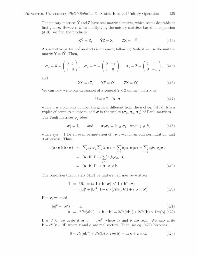
Princeton University Ph410 Solution 3. States, Bits and Unitary Operations 135
The unitary matrices Y and Z have real matrix elements, which seems desirable atfirst glance. However, when multiplying the unitary matrices based on expansion(413), we find the products
XY = Z, YZ = X, ZX = −Y. (414)
A symmetric pattern of products is obtained, following Pauli, if we use the unitarymatrix Y = iY. Then,
σx = X =
⎛⎝ 0 1
1 0
⎞⎠ , σy = Y =
⎛⎝ 0 −ii 0
⎞⎠ , σz = Z =
⎛⎝ 1 0
0 −1
⎞⎠ , (415)
andXY = iZ, YZ = iX, ZX = iY. (416)
We can now write our expansion of a general 2 × 2 unitary matrix as
U = a I + b · σ, (417)
where a is a complex number (in general different from the a of eq. (413)), b is atriplet of complex numbers, and σ is the triplet (σx,σy,σz) of Pauli matrices.
The Pauli matrices σj obey
σ2j = I, and σjσk = iεjkl σl when j = k, (418)
where εjkl = 1 for an even permutation of xyz, −1 for an odd permutation, and0 otherwise. Thus,
(a · σ)(b · σ) =∑j
aj σj∑k
bk σk =∑j=k
ajbk σjσk +∑j =k
ajbk σjσk
= (a · b) I + i∑j =k
ajbkεjkl σl
= (a · b) I + i σ · a × b. (419)
The condition that matrix (417) be unitary can now be written
I = UU† = (a I + b · σ)(a� I + b� · σ)
= (|a|2 + |b|2) I + σ · [2Re(ab�) + i b× b�]. (420)
Hence, we need
(|a|2 + |b|2) = 1, (421)
0 = 2Re(ab�) + i b × b� = 2Re(ab�) + 2Re(b) × Im(b).(422)
If a = 0, we write it as a = a0eiδ where a0 and δ are real. We also write
b = eiδ(c + id) where c and d are real vectors. Then, we eq. (422) becomes
0 = Re(ab�) +Re(b) × Im(b) = a0 c + c × d, (423)
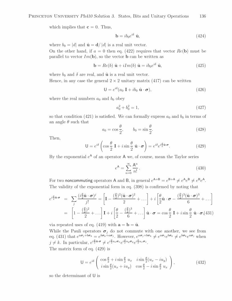
Princeton University Ph410 Solution 3. States, Bits and Unitary Operations 136
which implies that c = 0. Thus,
b = ib0eiδ u, (424)
where b0 = |d| and u = d/ |d| is a real unit vector.
On the other hand, if a = 0 then eq. (422) requires that vector Re(b) must beparallel to vector Im(b), so the vector b can be written as
b = Re(b) u + iIm(b) u = ib0eiδ u, (425)
where b0 and δ are real, and u is a real unit vector.
Hence, in any case the general 2 × 2 unitary matrix (417) can be written
U = eiδ(a0 I + ib0 u ·σ), (426)
where the real numbers a0 and b0 obey
a20 + b20 = 1, (427)
so that condition (421) is satisfied. We can formally express a0 and b0 in terms ofan angle θ such that
a0 = cosθ
2, b0 = sin
θ
2. (428)
Then,
U = eiδ(
cosθ
2I + i sin
θ
2u · σ
)= eiδei
θ2u·σ. (429)
By the exponential eA of an operator A we, of course, mean the Taylor series
eA =∞∑n=0
An
n!. (430)
For two noncommuting operators A and B, in general eA+B = eB+A = eAeB = eBeA.
The validity of the exponential form in eq. (398) is confirmed by noting that
eiθ2u·σ =
∑j
(i θ2u · σ)j
j!=
[I − ( θ
2)2(u · σ)2
2+ . . .
]+ i
[θ
2u · σ − ( θ
2)3(u · σ)3
6+ . . .
]
=
[1 − ( θ
2)2
2+ . . .
]I + i
[θ
2− ( θ
2)3
6+ . . .
]u · σ = cos
θ
2I + i sin
θ
2u · σ,(431)
via repeated uses of eq. (419) with a = b = u.
While the Pauli operators σj do not commute with one another, we see fromeq. (431) that eaσj+bσk = ebσk+aσj . However, eaσj+bσk = eaσjebσk = ebσkeaσj when
j = k. In particular, eiθ2u·σ = ei
θ2uxσxei
θ2uyσyei
θ2uzσz .
The matrix form of eq. (429) is
U = eiδ
⎛⎝ cos θ
2+ i sin θ
2ux i sin θ
2(ux − iuy)
i sin θ2(ux + iuy) cos θ
2− i sin θ
2ux
⎞⎠ , (432)
so the determinant of U is

Princeton University Ph410 Solution 3. States, Bits and Unitary Operations 137
ΔU = e2iδ
[cos2 θ
2+ sin2 θ
2
(u2x + u2
y + u2z
)]= e2iδ. (433)
Hence, the 2 × 2 special unitary operators (those for which ΔU = 1) are thosewith δ = 0 or π,
U = ±(
cosθ
2I + i sin
θ
2u · σ
)= ±ei θ
2u·σ, U ∈ SU(2). (434)
We note that the√
NOT operator, eq. (410), has determinant ±i, and so is nota special unitary operator.
As to the factoid related to eq. (38), whenever A2 = I we can make the Taylorexpansion,
eiθA =∞∑
k even
(iθA)k
k!+
∞∑k odd
(iθA)k
k!=
∞∑k even
(−1)k/2θk
k!I + i
∞∑k odd
(−1)(k−1)/2θk
k!A
= cos θ I + i sin θ A. (435)
(d) Applying the Z gate to classical bits |0〉 and |1〉 we have,
Z|0〉 =
⎛⎝ 1 0
0 −1
⎞⎠⎛⎜⎝ 1
0
⎞⎟⎠ = |0〉, Z|1〉 =
⎛⎝ 1 0
0 −1
⎞⎠⎛⎜⎝ 0
−1
⎞⎟⎠ = −|1〉. (436)
In a classical context, the state −|1〉 is either not defined, or could be considered asidentical to |1〉. Either way, the Z operator does not produce a result on classicalbits different from the two valid unitary operations I and X (N. Hu, 9/22/16).
In contrast, the effect of Z on a general Qbit |ψ〉 = a|0〉 + b|1〉 is nontrivial,
Z|ψ〉 =
⎛⎝ 1 0
0 −1
⎞⎠⎛⎜⎝ a
b
⎞⎟⎠ =
⎛⎜⎝ a
−b
⎞⎟⎠ . (437)
(e) 2-Bit Classical Unitary Operators
In part (a) we deduced that there are (2n)! classical unitary operators that act onn bits. Hence, there are (22)! = 4! = 24 classical 2-bit unitary operators.
In the form ⎛⎝ x
y
⎞⎠ →
⎛⎝ x′
y′
⎞⎠ = M
⎛⎝ x
y
⎞⎠⊕
⎛⎝ a
b
⎞⎠ , (438)
M is a 2× 2 invertible matrix, a and b are constant Cbits, and x, y, x′ and y′ arevariable Cbits.
If the output quantities x′ and y′ of eq. (438) are to be Cbits, the elementsof matrix M can only be 0’s or 1’s. With this constraint, the transformation

Princeton University Ph410 Solution 3. States, Bits and Unitary Operations 138
eq. (438) is automatically unitary, in that it takes a pair of Cbits into anotherpair of Cbits.138
Since the 2 × 2 matrix M has 4 elements, each 0 or 1, there are 24 = 16 differentM’s. The additional requirement that M be invertible implies that the determinantof M is nonzero. This eliminates those M’s in which the rows are identical, or inwhich the columns are identical, or in which a row or column contains only 0’s.The excluded matrices are⎛
⎝ 1 1
1 1
⎞⎠ ,
⎛⎝ 0 0
0 0
⎞⎠ ,
⎛⎝ 0 0
1 1
⎞⎠ ,
⎛⎝ 1 1
0 0
⎞⎠ ,
⎛⎝ 0 1
0 1
⎞⎠ ,
⎛⎝ 1 0
1 0
⎞⎠ ,
⎛⎝ 1 0
0 0
⎞⎠ ,
⎛⎝ 0 1
0 0
⎞⎠ ,
⎛⎝ 0 0
1 0
⎞⎠ ,
⎛⎝ 0 0
0 1
⎞⎠ , (439)
which leaves six viable versions of M, of which only the first two are unitary:⎛⎝ 1 0
0 1
⎞⎠ ,
⎛⎝ 0 1
1 0
⎞⎠ ,
⎛⎝ 0 1
1 1
⎞⎠ ,
⎛⎝ 1 0
1 1
⎞⎠ ,
⎛⎝ 1 1
0 1
⎞⎠ ,
⎛⎝ 1 1
1 0
⎞⎠ . (440)
There are, of course, four versions of the constant Cbit vector,⎛⎝ 1
1
⎞⎠ ,
⎛⎝ 0
0
⎞⎠ ,
⎛⎝ 1
0
⎞⎠ ,
⎛⎝ 0
1
⎞⎠ . (441)
Hence, there are 6×4 = 24 version of the linear, unitary transformation eq. (438),which exhausts the number of 2-bit classical unitary operators.
For the record, these 24 operators can be expressed as the 4 × 4 matrices⎛⎜⎝
1 0 0 0
0 1 0 0
0 0 1 0
0 0 0 1
⎞⎟⎠ ,
⎛⎜⎝
0 1 0 0
1 0 0 0
0 0 1 0
0 0 0 1
⎞⎟⎠ ,
⎛⎜⎝
0 0 1 0
0 1 0 0
1 0 0 0
0 0 0 1
⎞⎟⎠ ,
⎛⎜⎝
0 0 0 1
0 1 0 0
0 0 1 0
1 0 0 0
⎞⎟⎠ ,
⎛⎜⎝
1 0 0 0
0 1 0 0
0 0 0 1
0 0 1 0
⎞⎟⎠ ,
⎛⎜⎝
0 1 0 0
1 0 0 0
0 0 0 1
0 0 1 0
⎞⎟⎠ ,
⎛⎜⎝
0 0 0 1
0 1 0 0
1 0 0 0
0 0 1 0
⎞⎟⎠ ,
⎛⎜⎝
0 0 1 0
0 1 0 0
0 0 0 1
1 0 0 0
⎞⎟⎠ ,
⎛⎜⎝
1 0 0 0
0 0 1 0
0 1 0 0
0 0 0 1
⎞⎟⎠ ,
⎛⎜⎝
0 0 1 0
1 0 0 0
0 1 0 0
0 0 0 1
⎞⎟⎠ ,
⎛⎜⎝
0 1 0 0
0 0 1 0
1 0 0 0
0 0 0 1
⎞⎟⎠ ,
⎛⎜⎝
0 0 0 1
0 0 1 0
0 1 0 0
1 0 0 0
⎞⎟⎠ ,
⎛⎜⎝
1 0 0 0
0 0 0 1
0 1 0 0
0 0 1 0
⎞⎟⎠ ,
⎛⎜⎝
0 0 0 1
1 0 0 0
0 1 0 0
0 0 1 0
⎞⎟⎠ ,
⎛⎜⎝
0 1 0 0
0 0 0 1
1 0 0 0
0 0 1 0
⎞⎟⎠ ,
⎛⎜⎝
0 0 1 0
0 0 0 1
0 1 0 0
1 0 0 0
⎞⎟⎠ ,
⎛⎜⎝
1 0 0 0
0 0 1 0
0 0 0 1
0 1 0 0
⎞⎟⎠ ,
⎛⎜⎝
0 0 1 0
1 0 0 0
0 0 0 1
0 1 0 0
⎞⎟⎠ ,
⎛⎜⎝
0 0 0 1
0 0 1 0
1 0 0 0
0 1 0 0
⎞⎟⎠ ,
⎛⎜⎝
0 1 0 0
0 0 1 0
0 0 0 1
1 0 0 0
⎞⎟⎠ ,
138The use of addition modulo 2 in eq. (438) implies that 1 + 1 = 0, so that the sum of any two Cbits isstill a Cbit.

Princeton University Ph410 Solution 3. States, Bits and Unitary Operations 139
⎛⎜⎝
1 0 0 0
0 0 0 1
0 0 1 0
0 1 0 0
⎞⎟⎠ ,
⎛⎜⎝
0 0 0 1
1 0 0 0
0 0 1 0
0 1 0 0
⎞⎟⎠ ,
⎛⎜⎝
0 0 1 0
0 0 0 1
1 0 0 0
0 1 0 0
⎞⎟⎠ ,
⎛⎜⎝
0 1 0 0
0 0 0 1
0 0 1 0
1 0 0 0
⎞⎟⎠ . (442)
However, the matrix forms (442) obscure the fact that the 2-bit classical unitaryoperators are linear functions of the bits.
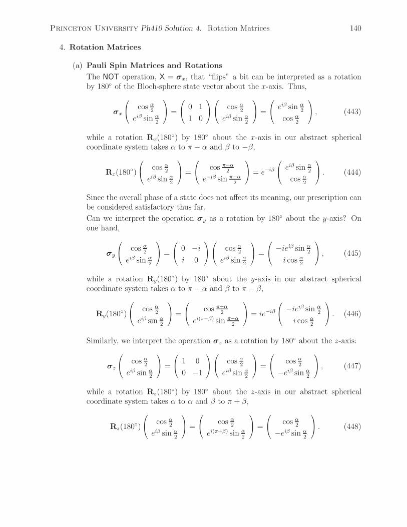
Princeton University Ph410 Solution 4. Rotation Matrices 140
4. Rotation Matrices
(a) Pauli Spin Matrices and Rotations
The NOT operation, X = σx, that “flips” a bit can be interpreted as a rotationby 180◦ of the Bloch-sphere state vector about the x-axis. Thus,
σx
⎛⎝ cos α
2
eiβ sin α2
⎞⎠ =
⎛⎝ 0 1
1 0
⎞⎠⎛⎝ cos α
2
eiβ sin α2
⎞⎠ =
⎛⎝ eiβ sin α
2
cos α2
⎞⎠ , (443)
while a rotation Rx(180◦) by 180◦ about the x-axis in our abstract spherical
coordinate system takes α to π − α and β to −β,
Rx(180◦)
⎛⎝ cos α
2
eiβ sin α2
⎞⎠ =
⎛⎝ cos π−α
2
e−iβ sin π−α2
⎞⎠ = e−iβ
⎛⎝ eiβ sin α
2
cos α2
⎞⎠ . (444)
Since the overall phase of a state does not affect its meaning, our prescription canbe considered satisfactory thus far.
Can we interpret the operation σy as a rotation by 180◦ about the y-axis? Onone hand,
σy
⎛⎝ cos α
2
eiβ sin α2
⎞⎠ =
⎛⎝ 0 −ii 0
⎞⎠⎛⎝ cos α
2
eiβ sin α2
⎞⎠ =
⎛⎝ −ieiβ sin α
2
i cos α2
⎞⎠ , (445)
while a rotation Ry(180◦) by 180◦ about the y-axis in our abstract spherical
coordinate system takes α to π − α and β to π − β,
Ry(180◦)
⎛⎝ cos α
2
eiβ sin α2
⎞⎠ =
⎛⎝ cos π−α
2
ei(π−β) sin π−α2
⎞⎠ = ie−iβ
⎛⎝ −ieiβ sin α
2
i cos α2
⎞⎠ . (446)
Similarly, we interpret the operation σz as a rotation by 180◦ about the z-axis:
σz
⎛⎝ cos α
2
eiβ sin α2
⎞⎠ =
⎛⎝ 1 0
0 −1
⎞⎠⎛⎝ cos α
2
eiβ sin α2
⎞⎠ =
⎛⎝ cos α
2
−eiβ sin α2
⎞⎠ , (447)
while a rotation Rz(180◦) by 180◦ about the z-axis in our abstract spherical
coordinate system takes α to α and β to π + β,
Rz(180◦)
⎛⎝ cos α
2
eiβ sin α2
⎞⎠ =
⎛⎝ cos α
2
ei(π+β) sin α2
⎞⎠ =
⎛⎝ cos α
2
−eiβ sin α2
⎞⎠ . (448)

Princeton University Ph410 Solution 4. Rotation Matrices 141
(b) Rotation and Pauli Spin Matrices
The rotations (45)-(47) are readily seen to be exponentials of the Pauli matrices,
Rx(φ) =
⎛⎝ cos φ
2i sin φ
2
i sin φ2
cos φ2
⎞⎠ = cos
φ
2I + i sin
φ
2σx = ei
φ2σx, (449)
Ry(φ) =
⎛⎝ cos φ
2sin φ
2
− sin φ2
cos φ2
⎞⎠ = cos
φ
2I + i sin
φ
2σy = ei
φ2σy , (450)
Rz(φ) =
⎛⎝ eiφ/2 0
0 e−iφ/2
⎞⎠ = cos
φ
2I + i sin
φ
2σz = ei
φ2σz , (451)
recalling eq. (37).
The αth power of the Pauli matrix σz follows from eq. (54) as
σαz = Zα = (eiπ2 e−i
π2σz)α = ei
πα2 e−i
πα2
σz = eiπα2
[I cos
−πα2
+ iσz sin−πα
2
]
= eiπα2
⎛⎝ cos −πα
2+ i sin −πα
20
0 cos πα2
+ i sin πα2
⎞⎠
= eiπα2
⎛⎝ e−i
πα2 0
0 eiπα2
⎞⎠ =
⎛⎝ 1 0
0 eiπα
⎞⎠ . (452)
(c) More Square Roots of NOT
If we take the NOT operation to mean flipping a bit with a possible phase change,we can accomplish this by a rotation by 180◦ about any axis in the x-y plane ofthe Bloch sphere. The corresponding
√NOT operation would be a rotation by
90◦ about the same axis.
Consider an axis y1 in the x-y plane that makes angle α to the y-axis. A prescrip-tion for rotation by angle φ about the y1-axis, based on the general procedure(44), is to make a rotation by α about the z axis, followed by a rotation by φabout the y1-axis, and finally a rotation by −α about the z′ axis:
Ry1(φ) = R(α, φ,−α) =
⎛⎝ cos(φ/2) sin(φ/2)e−iα
− sin(φ/2)eiα cos(φ/2)
⎞⎠ (453)
Note that using α = −π/2 in eq. (453) gives the matrix (45) for rotations aboutthe x-axis.
Putting φ = π and π/2 in eq. (453) we obtain new expressions for the NOT and√NOT operators:
NOT = Ry1(π) =
⎛⎝ 0 e−iα
−eiα 0
⎞⎠ , (454)
√NOT = Ry1(π/2) =
1√2
⎛⎝ 1 e−iα
−eiα 1
⎞⎠ . (455)
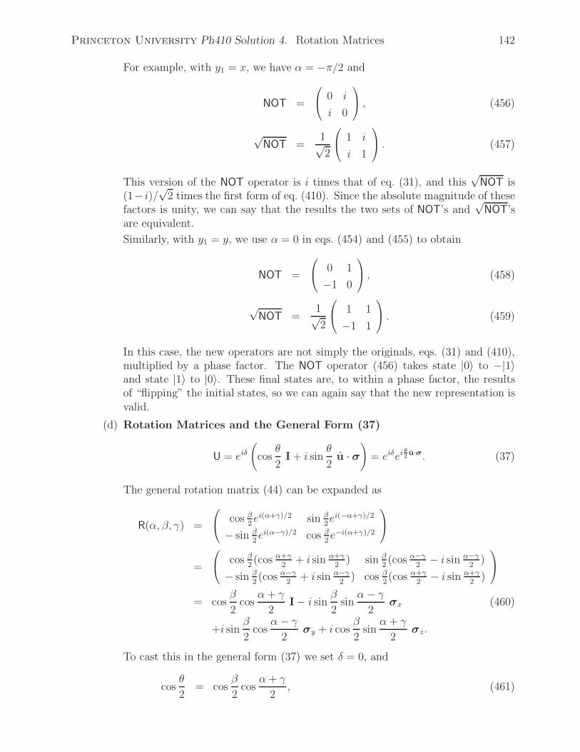
Princeton University Ph410 Solution 4. Rotation Matrices 142
For example, with y1 = x, we have α = −π/2 and
NOT =
⎛⎝ 0 i
i 0
⎞⎠ , (456)
√NOT =
1√2
⎛⎝ 1 i
i 1
⎞⎠ . (457)
This version of the NOT operator is i times that of eq. (31), and this√
NOT is(1− i)/√2 times the first form of eq. (410). Since the absolute magnitude of thesefactors is unity, we can say that the results the two sets of NOT’s and
√NOT’s
are equivalent.
Similarly, with y1 = y, we use α = 0 in eqs. (454) and (455) to obtain
NOT =
⎛⎝ 0 1
−1 0
⎞⎠ , (458)
√NOT =
1√2
⎛⎝ 1 1
−1 1
⎞⎠ . (459)
In this case, the new operators are not simply the originals, eqs. (31) and (410),multiplied by a phase factor. The NOT operator (456) takes state |0〉 to −|1〉and state |1〉 to |0〉. These final states are, to within a phase factor, the resultsof “flipping” the initial states, so we can again say that the new representation isvalid.
(d) Rotation Matrices and the General Form (37)
U = eiδ(
cosθ
2I + i sin
θ
2u · σ
)= eiδei
θ2u·σ. (37)
The general rotation matrix (44) can be expanded as
R(α, β, γ) =
⎛⎝ cos β
2ei(α+γ)/2 sin β
2ei(−α+γ)/2
− sin β2ei(α−γ)/2 cos β
2e−i(α+γ)/2
⎞⎠
=
⎛⎝ cos β
2(cos α+γ
2+ i sin α+γ
2) sin β
2(cos α−γ
2− i sin α−γ
2)
− sin β2(cos α−γ
2+ i sin α−γ
2) cos β
2(cos α+γ
2− i sin α+γ
2)
⎞⎠
= cosβ
2cos
α+ γ
2I − i sin
β
2sin
α− γ
2σx (460)
+i sinβ
2cos
α − γ
2σy + i cos
β
2sin
α+ γ
2σz.
To cast this in the general form (37) we set δ = 0, and
cosθ
2= cos
β
2cos
α+ γ
2, (461)
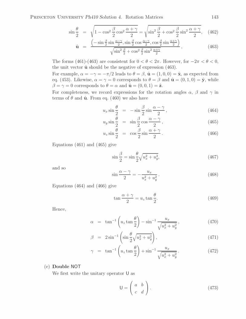
Princeton University Ph410 Solution 4. Rotation Matrices 143
sinθ
2=
√1 − cos2
β
2cos2
α + γ
2=
√sin2 β
2+ cos2
β
2sin2 α+ γ
2, (462)
u =
(− sin β
2sin α−γ
2, sin β
2cos α−γ
2, cos β
2sin α+γ
2
)√
sin2 β2
+ cos2 β2sin2 α+γ
2
, (463)
The forms (461)-(463) are consistent for 0 < θ < 2π. However, for −2π < θ < 0,the unit vector u should be the negative of expression (463).
For example, α = −γ = −π/2 leads to θ = β, u = (1, 0, 0) = x, as expected fromeq. (453). Likewise, α = γ = 0 corresponds to θ = β and u = (0, 1, 0) = y, whileβ = γ = 0 corresponds to θ = α and u = (0, 0, 1) = z.
For completeness, we record expressions for the rotation angles α, β and γ interms of θ and u. From eq. (460) we also have
ux sinθ
2= − sin
β
2sin
α− γ
2, (464)
uy sinθ
2= sin
β
2cos
α − γ
2, (465)
uz sinθ
2= cos
β
2sin
α + γ
2. (466)
Equations (461) and (465) give
sinβ
2= sin
θ
2
√u2x + u2
y, (467)
and so
sinα − γ
2= − ux
u2x + u2
y
. (468)
Equations (464) and (466) give
tanα + γ
2= uz tan
θ
2. (469)
Hence,
α = tan−1
(uz tan
θ
2
)− sin−1 ux√
u2x + u2
y
, (470)
β = 2 sin−1
(sin
θ
2
√u2x + u2
y
), (471)
γ = tan−1
(uz tan
θ
2
)+ sin−1 ux√
u2x + u2
y
. (472)
(e) Double NOT
We first write the unitary operator U as
U =
⎛⎝ a b
c d
⎞⎠ . (473)

Princeton University Ph410 Solution 4. Rotation Matrices 144
Then
XUX =
⎛⎝ 0 1
1 0
⎞⎠⎛⎝ a b
c d
⎞⎠⎛⎝ 0 1
1 0
⎞⎠ =
⎛⎝ 0 1
1 0
⎞⎠⎛⎝ b a
d c
⎞⎠ =
⎛⎝ d c
b a
⎞⎠ . (474)
Writing
U = eiδR(α, β, γ) = eiδ
⎛⎝ cos(β/2)ei(α+γ)/2 sin(β/2)ei(−α+γ)/2
− sin(β/2)ei(α−γ)/2 cos(β/2)e−i(α+γ)/2
⎞⎠ , (475)
and recalling eq. (460), we see that
XUX = eiδ
⎛⎝ cos(β/2)e−i(α+γ)/2 − sin(β/2)ei(α−γ)/2
sin(β/2)ei(−α+γ)/2 cos(β/2)ei(α+γ)/2
⎞⎠ = eiδR(−α,−β,−γ). (476)
(f) Basis Change
Since U is unitary, we have
U†U =
⎛⎝ a� c�
b� d�
⎞⎠⎛⎝ a b
c d
⎞⎠ =
⎛⎝ |a|2 + |c|2 a�b+ c�d
ab� + cd� |b|2 + |d|2⎞⎠ =
⎛⎝ 1 0
0 1
⎞⎠ . (477)
Thus the states
|ψ〉 = U|0〉 = a|0〉 + c|1〉, |φ〉 = U|1〉 = b|0〉 + d|1〉. (478)
obey
〈ψ|ψ〉 = |a|2 + |c|2 = 1, or 〈ψ|ψ〉 = 〈0|U†U|0〉 = 〈0|0〉 = 1, (479)
〈φ|φ〉 = |b|2 + |d|2 = 1, or 〈φ|φ〉 = 〈1|U†U|1〉 = 〈1|1〉 = 1, (480)
〈ψ|φ〉 = a�b+ c�d = 0, or 〈ψ|φ〉 = 〈0|U†U|1〉 = 〈0|1〉 = 0, (481)
and so they are orthonormal as claimed.
(g) Hadamard Transformation
The Hadamard transformation,
H =1√2
⎛⎝ 1 1
1 −1
⎞⎠ =
X + Z√2
=σx + σz√
2, (482)
has determinant ΔH = −1 = e2iδ, where eiδ is the phase factor in the generalforms (37) and (56),
U = eiδ(
cosθ
2I + i sin
θ
2u · σ
)= eiδei
θ2u·σ, (37)
U = eiδR(α, β, γ) = eiδRz(γ)Ry(β)Rz(α). (56)

Princeton University Ph410 Solution 4. Rotation Matrices 145
Thus, δ = ±π/2.We first examine that case that δ = π/2. To relate eq. (482) to the form (37), wewrite
H =σx + σz√
2= eiδ(−i)σx + σz√
2= eiδ(−iu · σ)
= eiδ[cos(−π/2) I + i sin(−π/2)u · σ] = eiδeiθ2u·σ, (483)
where
δ =π
2, θ = −π, and u =
(1, 0, 1)√2
. (484)
Because θ = −π, we must be careful to use the negative of expression eq. (463)for the unit vector u. First, we can set
α− γ
2=π
2(485)
to have uy = 0. Then to obtain ux = uz = 1/√
2 we need
sin β2
sin α−γ2√
sin2 β2
+ cos2 β2
sin2 α+γ2
=1√2
= − cos β2
sin α+γ2√
sin2 β2
+ cos2 β2
sin2 α+γ2
. (486)
This is satisfied by taking
β =π
2(487)
to have cos β2
= 1/√
2, andα+ γ
2= −π
2. (488)
Combining eqs. (485) and (488) we arrive at
α = 0, β =π
2, γ = −π, and δ =
π
2, (489)
so that the Hadamard transformation can also be written as
H = eiδR(α, β, γ) = eiπ/2Rz(−π)Ry
(−π
2
)
= i
⎛⎝ −i 0
0 i
⎞⎠⎛⎝ 1√
21√2
− 1√2
1√2
⎞⎠ =
1√2
⎛⎝ 1 1
1 −1
⎞⎠ . (490)
By setting δ = ±π/2 and α − γ = ±π we can obtain 3 more representations ofthe Hadamard transformation,
H = eiπ/2Ry
(−π
2
)Rz(−π) = e−iπ/2Ry
(−π
2
)Rz(π) = e−iπ/2Rz(π)Ry
(π
2
). (491)

Princeton University Ph410 Solution 4. Rotation Matrices 146
(h) The αth power of the Pauli matrix σx follows from eq. (54) as
σαx = eiπα2 e−i
πα2
σx = eiπα2 [I cos(πα/2) − iσx sin(πα/2)]
=e−i
πα2
2
[I(ei
πα2 + e−i
πα2 ) − σx(eiπα
2 − e−iπα2 )]
=1
2
[I(eiπα + 1) − σx(eiπα − 1)
]
=1
2
⎛⎝ 1 + eiπα 1 − eiπα
1 − eiπα 1 + eiπα
⎞⎠ . (492)
Meanwhile, we have
HσαzH =1
2
⎛⎝ 1 1
1 −1
⎞⎠⎛⎝ 1 0
0 eiπα
⎞⎠⎛⎝ 1 1
1 −1
⎞⎠
=1
2
⎛⎝ 1 + eiπα 1 − eiπα
1 − eiπα 1 + eiπα
⎞⎠ = σαx . (493)
Similarly,
σαy = eiπα2 e−i
πα2
σy =1
2
[I(eiπα + 1) − σy(eiπα − 1)
]
=1
2
⎛⎝ 1 + eiπα −i(1 − eiπα)
i(1 − eiπα) 1 + eiπα
⎞⎠ , (494)
while
σ1/2z σαxσ
−1/2z =
1
2
⎛⎝ 1 0
0 i
⎞⎠⎛⎝ 1 + eiπα 1 − eiπα
1 − eiπα 1 + eiπα
⎞⎠⎛⎝ 1 0
0 −i
⎞⎠
=1
2
⎛⎝ 1 + eiπα −i(1 − eiπα)
i(1 − eiπα) 1 + eiπα
⎞⎠ = σαy . (495)
Using eqs. (483)-(484) we can write the Hadamard transformation in exponentialform as139
H = eiπ2 e
−i π2√
2(σx+σz)
= eiπ2 e−i
π2H, (496)
so the αth power of this is
Hα = eiπα2 e−i
πα2
H = eiπα2 [I cos(πα/2) − iH sin(πα/2)]
=ei
πα2
2
[I(ei
πα2 + e−i
πα2 ) − H(ei
πα2 − e−i
πα2 )]
=1
2
[I(1 + eiπα) + H(1 − eiπα)
]
=1
2√
2
⎛⎝ √
2 + 1 + (√
2 − 1)eiπα 1 − eiπα
1 − eiπα√
2 − 1 + (√
2 + 1)eiπα
⎞⎠ , (497)
139This also follows from eq. (38).

Princeton University Ph410 Solution 4. Rotation Matrices 147
while
σ1/4y σαzσ
−1/4y =
1
8
⎛⎝ √
2 + 1 + i −1 − i(√
2 − 1)
1 + i(√
2 − 1)√
2 + 1 + i
⎞⎠⎛⎝ 1 0
0 eiπα
⎞⎠
⎛⎝ √
2 + 1 − i 1 − i(√
2 − 1)
−1 + i(√
2 − 1)√
2 + 1 − i
⎞⎠
=1
2√
2
⎛⎝ √
2 + 1 + (√
2 − 1)eiπα 1 − eiπα
1 − eiπα√
2 − 1 + (√
2 + 1)eiπα
⎞⎠
= Hα. (498)
(i) To characterize the product
H−1/2 eiθ2u·σ H1/2, (499)
we note from eq. (497) that
H±1/2 = e±iπ4 e∓i
π4H = e±i
π4 [cos(π/4)I ∓ i sin(π/4)H] =
e±iπ4√2
[I ∓ iH]. (500)
Thus,
H−1/2 eiθ2u·σ H1/2 =
1
2[I + iH][cos(θ/2)I + i sin(θ/2)u · σ][I− iH] (501)
= cos(θ/2)I +i
2sin(θ/2)[u ·σ + u · HσH − iu · σH + iu · Hσ].
We would now like to show that the quantity in brackets in the second line ofeq. (501) can be written as 2v ·σ. For this, we recall that H = (σx +σz)/
√2 and
the facts that σ2j = I and σjσk = iεjklσl when j = k to accumulate the following
relations:
σxH = σxσx + σz√
2=
I − iσy√2
, Hσx =I + iσy√
2,
HσxH =σx + σz − i(σx + σz)σy
2= σz, σxH − Hσx = −
√2iσy, (502)
σyH = σyσx + σz√
2= i
−σz + σx√2
, Hσy = iσz −σx√
2,
HσyH = i(σx + σz)(σx − σz)
2= −σy, σyH −Hσy =
√2i(σx − σz), (503)
σzH = σzσx + σz√
2=iσy + I√
2, Hσz =
−iσy + I√2
,
HσzH =i(σx + σz)σy + σx + σz
2= σx, σzH − Hσz =
√2iσy, (504)

Princeton University Ph410 Solution 4. Rotation Matrices 148
Using eqs. (502)-(504) in eq. (501) we find that
u · σ + u · HσH − iu · (σH −Hσ) = uxσx + uyσy + uzσz
uxσz − uyσy + uzσx
+√
2[−uxσy + uy(σx −σx) + uzσy]
= σx(ux +√
2uy + uz) −√
2σy(ux − uz)
+σz(ux −√
2uy + uz)
= 2v · σ, (505)
where
v =(ux +
√2uy + uz,−
√2(ux − uz), ux −
√2uy + uz)
2. (506)
The vector v is readily verified to be a unit vector, while
u · v = (ux + uz)2. (507)
Hence,
H−1/2 eiθ2u·σ H1/2 = ei
θ2v·σ, (508)
where v is orthogonal to u provided uz = −ux.(j) Basis States for the Hadamard Transformation140
We seek all orthonormal bases [|ψ〉, |φ〉] for which
H|ψ〉 =|ψ〉 + |φ〉√
2, and H|φ〉 =
|ψ〉 − |φ〉√2
. (68)
where the basis states are described as unit vectors on the Bloch sphere,
|ψ〉 = cosα
2|0〉 + eiβ sin
α
2|1〉, (42)
|φ〉 = eiδ[sin
α
2|0〉 − eiβ cos
α
2|1〉]. (69)
Inserting eqs. (42) and (69) into the first of eq. (68), we find
[cos
α
2+ eiβ sin
α
2
] |0〉√2
+[cos
α
2− eiβ sin
α
2
] |1〉√2
=[cos
α
2+ eiδ sin
α
2
] |0〉√2
+[−ei(β+δ) cos
α
2+ eiβ sin
α
2
] |1〉√2. (509)
Equating the coefficients of |0〉 we see that β = δ, while from the coefficients of|1〉 we find
cosα
2(1 + e2iβ) = 2eiβ sin
α
2, (510)
and hence,
cos β = tanα
2=
1 − cosα
sinα. (511)
140 http://physics.princeton.edu/~mcdonald/examples/QM/maitra_quant-ph-0505068.pdf

Princeton University Ph410 Solution 4. Rotation Matrices 149
Use of the second of eq. (68) leads to the same result.
The solution to eq. (511) includes |ψ〉 = |0〉 with α = 0, β = ±π/2, and |ψ〉 = |+〉with α = π/2, β = 0. To see that the general solution, eq. (511), sweeps out acone whose axis lies in the x-z plane at 45◦ to the x and z axes, it is helpful towrite down the rectangular coordinates of the vector |φ〉 on the unit Bloch sphere,
x = sinα cosβ = 1 − cosα, (512)
y = sinα sinβ =√
2(cosα − cos2 α), (513)
z = cosα. (514)
If we rotate the coordinates by 45◦ about the y axis into the (x′, y′, z′) system, wehave
x′ =x− z√
2=
1 − 2 cos α√2
, (515)
y′ = y =√
2(cosα− cos2 α), (516)
z′ =x+ z√
2=
1√2. (517)
Thus, the solution to eq. (511) in the (x′, y′, z′) coordinate system is the inter-section of the unit sphere with the plane z′ = 1/
√2, which is a circle of radius
r =√x′2 + y′2 = 1/
√2. That is, the solution-states |ψ〉 sweep out a cone of half
angle 45◦ about the z′ axis.

Princeton University Ph410 Solution 5. Measurements 150
5. Measurements
(a) Expressing the operator v · σ as a matrix, we have
v · σ =
⎛⎝ vz vx − ivy
vx + ivy −vz
⎞⎠ . (518)
The eigenvalues λ satisfy the equation
v · σ|ψ〉 = λ|ψ〉, (519)
which implies that
0 = Δ(v · σ − λI) =
∣∣∣∣∣∣vz − λ vx − ivy
vx + ivy −vz − λ
∣∣∣∣∣∣ = λ2 − v2z − v2
x − v2y = λ2 − 1, (520)
so the eigenvalues areλ = ±1. (521)
To find the eigenvectors, we recall the relations between the Pauli spin matricesand rotations. Thus, we expect that the eigenvectors of operator v · σ are the|0〉 and |1〉 states that correspond to the direction of the unit vector v. Recallingeq. (42), we anticipate that one of the eigenvectors is the state
|+〉 = cos(α/2)|0〉 + eiβ sin(α/2)|1〉, (522)
where the angles α and β are given by
vx = sinα cosβ, vy = sinα sinβ, vz = cosα. (523)
We verify this, expressing the matrix (518) in terms of α and β,
v · σ|+〉 =
⎛⎝ cosα e−iβ sinα
eiβ sinα − cosα
⎞⎠⎛⎝ cos(α/2)
eiβ sin(α/2)
⎞⎠
=
⎛⎝ cosα cos(α/2) + sinα sin(α/2)
eiβ sinα cos(α/2) − eiβ cosα sin(α/2)
⎞⎠
=
⎛⎝ cos(α− α/2)
eiβ sin(α − α/2)
⎞⎠ =
⎛⎝ cos(α/2)
eiβ sin(α/2)
⎞⎠ = +1 · |+〉. (524)
The other eigenstate, |−〉, is orthogonal to |+〉. From eq. (522) we infer that
|−〉 = e−iβ sin(α/2)|0〉 − cos(α/2)|1〉, (525)

Princeton University Ph410 Solution 5. Measurements 151
as is readily verified:
v · σ|−〉 =
⎛⎝ cosα e−iβ sinα
eiβ sinα − cosα
⎞⎠⎛⎝ e−iβ sin(α/2)
− cos(α/2)
⎞⎠
=
⎛⎝ e−iβ cosα sin(α/2) − e−iβ sinα cos(α/2)
sinα sin(α/2) + cosα cos(α/2)
⎞⎠
=
⎛⎝ −e−iβ sin(α− α/2)
cos(α − α/2)
⎞⎠ =
⎛⎝ −e−iβ sin(α/2)
−[− cos(α/2)]
⎞⎠ = −1 · |−〉. (526)
The projection operator for the |+〉 eigenstate is
P+ = |+〉〈+|= [cos(α/2)|0〉 + eiβ sin(α/2)|1〉][cos(α/2)〈0| + e−iβ sin(α/2)〈1|]= cos2(α/2)|0〉〈0| + e−iβ sin(α/2) cos(α/2)|0〉|1〉]
+eiβ sin(α/2) cos(α/2)|1〉|0〉] + sin2(α/2)|1〉〈1|
=
⎛⎝ cos2(α/2) e−iβ sin(α/2) cos(α/2)
eiβ sin(α/2) cos(α/2) sin2(α/2)
⎞⎠
=1
2
⎛⎝ 1 + cosα e−iβ sinα
eiβ sinα 1 − cosα
⎞⎠ =
I + v ·σ2
. (527)
Similarly,
P− = |−〉〈−| =
⎛⎝ e−iβ sin(α/2)
− cos(α/2)
⎞⎠( eiβ sin(α/2) − cos(α/2)
)
=
⎛⎝ sin2(α/2) −e−iβ sin(α/2) cos(α/2)
−eiβ sin(α/2) cos(α/2) cos2(α/2)
⎞⎠
=1
2
⎛⎝ 1 − cosα −e−iβ sinα
−eiβ sinα 1 + cosα
⎞⎠ =
I − v · σ2
. (528)
The probability that a state |ψ〉 will be found in the |+〉 state is
P+ = 〈ψ|P+|ψ〉. (529)
In particular, for the initial state |0〉
P+ = 〈0|P+|0〉 = P+,00 =1 + cosα
2=
1 + vz2
. (530)
If the initial state |ψ〉 is measured to be in the state |+〉, the final state is, ofcourse, the state |+〉 described by eq. (522).

Princeton University Ph410 Solution 5. Measurements 152
(b) The measurement operator to determine the value of the second bit of state |ψ〉can be written as
M2 = 0 · P0,2 + 1 · P1,2 = 0 · |0〉2〈0|2 + 1 · |1〉2〈1|2. (531)
Applying this to the state
|ψ〉 = ψ00|0〉|0〉 + ψ01|0〉|1〉 + ψ10|1〉|0〉 + ψ11|1〉|1〉, (532)
we obtain
M2|ψ〉 = 0 · (ψ00|0〉|0〉 + ψ10|1〉|0〉) + 1 · (ψ01|0〉|1〉 + ψ11|1〉|1〉). (533)
This means that the probability that the second bit is found to be |1〉 is
P2(1) = 〈ψ|P†1,2P1,2|ψ〉 = |ψ01|2 + |ψ11|2 , (534)
and that if this is the result, the state after the measurement is
|ψ′〉 =P1,2|ψ〉√
〈ψ|P†1,2P1,2|ψ〉
=ψ01|0〉|1〉 + ψ11|1〉|1〉√
|ψ01|2 + |ψ11|2. (535)
If the measurement does not yield the value 1 for the second bit, it yields thevalue 0. The probability of this outcome is
P2(0) = 〈ψ|P†1,2P1,2|ψ〉 = |ψ00|2 + |ψ10|2 = 1 − |ψ01|2 − |ψ11|2 = 1 − P2(1), (536)
and that if this is the result, the state after the measurement is
|ψ′〉 =P0,2|ψ〉√
〈ψ|P†0,2P0,2|ψ〉
=ψ00|0〉|0〉 + ψ10|1〉|0〉√
|ψ00|2 + |ψ10|2. (537)
If we wish to determine the value of both bits of state (532), we note that theoperators to determine if bits 1 and 2 have values j = 0 or 1 and k = 0 or 1 arePjk where
P00 = |0〉1〈0|1 ⊗ |0〉2〈0|2, (538)
P01 = |0〉1〈0|1 ⊗ |1〉2〈1|2, (539)
P10 = |1〉1〈1|1 ⊗ |0〉2〈0|2, (540)
P11 = |1〉1〈1|1 ⊗ |1〉2〈1|2, (541)
The eigenstates of these four operators are |0〉|0〉, |0〉|1〉, |1〉|0〉 and |1〉|1〉, and thecorresponding eigenvalues are all unity. However, if we simply add the four oper-ators with unit weights, we obtain the unit matrix. We construct a measurementoperator M12 that can distinguish the four eigenstates by summing the operators(538)-(541) with weights ranging from binary numbers 00 to 11 according to
M12 = 00 · P00 + 01 · P01 + 10 · P10 + 11 · P11. (542)

Princeton University Ph410 Solution 5. Measurements 153
Applying this to the state (532) we obtain
M12|ψ〉 = 00 · ψ00|0〉|1〉 + 01 · ψ01|0〉|1〉 + 10 · ψ10|1〉|0〉 + 11 · ψ11|1〉|1〉. (543)
We interpret this the with the aid of von Neumann’s argument as meaning thatthe four terms of eq. (543) are correlated with four positions of a pointer. Whenthe pointer is observed, it is found to be in one of the four positions. If themeasurement could be repeated with many copies of state |ψ〉 the probabilities
of observing the pointer would be∣∣∣ψjk∣∣∣2 for the position with binary number jk.
If the pointer is found to be at position jk, then we have measured bit 1 to havevalue j and bit 2 to have value k. The state of |ψ〉 after this measurement is|j〉|k〉.
(c) Stern-Gerlach
The property of the neutral spin-1/2 particle to be measured is the z componentof its spin, for which the relevant operator is σz.
The value of the pointer in the Stern-Gerlach apparatus is the angle of the trajec-tory of the particle in the x-z plane after is leaves the apparatus. This is equivalentto the pointer value being the z component of the particle’s momentum. So, wetake the “coordinate” to be measured as pz. The ”momentum” that is conjugateto pz is just the spatial coordinate z.
Therefore, we need a Hamiltonian of the form
h = λσzz, (544)
where z is the hermitian operator associated with the observable coordinate z.
Such a Hamiltonian can be realized by passing the particle through a magneticfield B. Then, its magnetic energy, U = −μ · B, where μ = γs = hγσ/2 is theparticle’s magnetic moment and σ = (σx,σy,σz) is the Pauli-matrix vector. The(reduced) interaction Hamiltonian h = H/h of the particle is
h = −γ2σ ·B. (545)
We make eq. (545) have the desired form (544) by choosing the magnetic field tobe in the z direction and to vary linearly with position,
B = −Azz, (546)
h =γA
2σzz. (547)
(d) Quantum Nondemolition Measurement
We desire the form of a unitary 4 × 4 matrix U that operates on Qbits |ψ〉 =a0|0〉 + a1|1〉 and |0〉 according to U|ψ〉|0〉 = a0|0〉|0〉 + a1|1〉|1〉.The initial state is
|ψ〉|0〉 = a0|0〉|0〉 + a1|1〉|0〉 =
⎛⎜⎜⎜⎜⎜⎜⎝
a0
0
a1
0
⎞⎟⎟⎟⎟⎟⎟⎠, (548)

Princeton University Ph410 Solution 5. Measurements 154
and the desired final state is
U|ψ〉|0〉 = U
⎛⎜⎜⎜⎜⎜⎜⎝
a0
0
a1
0
⎞⎟⎟⎟⎟⎟⎟⎠
=
⎛⎜⎜⎜⎜⎜⎜⎝
a0
0
0
a1
⎞⎟⎟⎟⎟⎟⎟⎠. (549)
A suitable 4 × 4 matrix representation of the unitary operator U is therefore
U =
⎛⎜⎜⎜⎜⎜⎜⎝
1 0 0 0
0 a 0 b
0 c 0 d
0 0 1 0
⎞⎟⎟⎟⎟⎟⎟⎠, (550)
noting that each row and column of a unitary matrix, considered as a vector, isnormalized to 1.
If U is symmetric, then d = 1. For the row and column containing d to benormalized, we have that b = c = 0, and finally, for the row and column continainga to be normalized we must have a = 1. Thus,
U =
⎛⎜⎜⎜⎜⎜⎜⎝
1 0 0 0
0 1 0 0
0 0 0 1
0 0 1 0
⎞⎟⎟⎟⎟⎟⎟⎠. (551)
The matrix U of eq. (551) will soon become our favorite 4 × 4 matrix, and hasbeen given the name Controlled-NOT or C-NOT.

Princeton University Ph410 Solution 6. Quantum Cloning and Teleportation 155
6. Quantum Cloning and Quantum Teleportation
(a) Quantum Cloning
The Controlled-NOT operator Cxy does nothing to |y〉 when |x = 0〉, so |0〉|0〉goes to |0〉|0〉 and |0〉|1〉 goes to |0〉|1〉, but flips |y〉 when |x = 1〉, so |1〉|0〉 goesto |1〉|1〉 and |1〉|1〉 goes to |1〉|0〉. These rules determine the matrix elements tobe
Cxy =
⎛⎜⎜⎜⎜⎜⎜⎝
1 0 0 0
0 1 0 0
0 0 0 1
0 0 1 0
⎞⎟⎟⎟⎟⎟⎟⎠
=
⎛⎝ I 0
0 X
⎞⎠ , (552)
The two-bit state (a|0〉 + b|1〉)|0〉 can be written as the column vector
v =
⎛⎜⎜⎜⎜⎜⎜⎝
a
0
b
0
⎞⎟⎟⎟⎟⎟⎟⎠. (553)
Applying transformation (552) to this we obtain
Cxyv =
⎛⎜⎜⎜⎜⎜⎜⎝
1 0 0 0
0 1 0 0
0 0 0 1
0 0 1 0
⎞⎟⎟⎟⎟⎟⎟⎠
⎛⎜⎜⎜⎜⎜⎜⎝
a
0
b
0
⎞⎟⎟⎟⎟⎟⎟⎠
=
⎛⎜⎜⎜⎜⎜⎜⎝
a
0
0
b
⎞⎟⎟⎟⎟⎟⎟⎠. (554)
However, if bit |y〉 were to be a copy of bit |x〉 we should have obtained the state
a|0〉 + b|1〉)a|0〉 + b|1〉) =
⎛⎜⎜⎜⎜⎜⎜⎝
a2
ab
ab
b2
⎞⎟⎟⎟⎟⎟⎟⎠. (555)
The two states (554) and (555) are equal only if ab = 0, in which case we musthave (a, b) = (1, 0) or (0, 1). That is, only cCbits can be copied successfully bythe Controlled-NOT operator.
By the definition of the Controlled-NOT operation, we have that Cxy|0〉|0〉 = |0〉|0〉and Cxy|1〉|1〉 = |1〉|0〉. Thus Cxy successfully deletes the second of a pair ofidentical Cbits. However, if we apply Cxy to a pair of identical Qbits, given byeq. (555), we find
Cxyv =
⎛⎜⎜⎜⎜⎜⎜⎝
1 0 0 0
0 1 0 0
0 0 0 1
0 0 1 0
⎞⎟⎟⎟⎟⎟⎟⎠
⎛⎜⎜⎜⎜⎜⎜⎝
a2
ab
ab
b2
⎞⎟⎟⎟⎟⎟⎟⎠
=
⎛⎜⎜⎜⎜⎜⎜⎝
a2
ab
b2
ab
⎞⎟⎟⎟⎟⎟⎟⎠, (556)
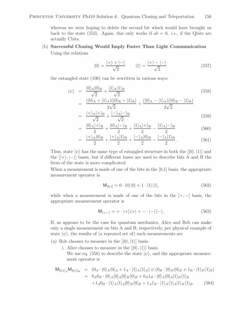
Princeton University Ph410 Solution 6. Quantum Cloning and Teleportation 156
whereas we were hoping to delete the second bit which would have brought usback to the state (553). Again, this only works if ab = 0, i.e., if the Qbits areactually Cbits.
(b) Successful Cloning Would Imply Faster Than Light Communication
Using the relations
|0〉 =|+〉 + |−〉√
2|1〉 =
|+〉 − |−〉√2
(557)
the entangled state (106) can be rewritten in various ways:
|ψ〉 =|0〉A|0〉B√
2+
|1〉A|1〉B√2
(558)
=(|0〉A + |1〉A)(|0〉B + |1〉B)
2√
2+
(|0〉A − |1〉A)(|0〉B − |1〉B)
2√
2
=|+〉A|+〉B√
2+
|−〉A|−〉B√2
(559)
=|0〉A|+〉B
2+
|0〉A|−〉B2
+|1〉A|+〉B
2− |1〉A|−〉B
2(560)
=|+〉A|0〉B
2+
|+〉A|1〉B2
+|−〉A|0〉B
2− |−〉A|1〉B
2. (561)
Thus, state |ψ〉 has the same type of entangled structure in both the [|0〉, |1〉] andthe [|+〉, |−〉] bases, but if different bases are used to describe bits A and B theform of the state is more complicated.
When a measurement is made of one of the bits in the [0,1] basis, the appropriatemeasurement operator is
M[0,1] = 0 · |0〉〈0| + 1 · |1〉〈1|, (562)
while when a measurement is made of one of the bits in the [+,−] basis, theappropriate measurement operator is
M[+,−] = + · |+〉〈+| + − · |−〉〈−|, (563)
If, as appears to be the case for quantum mechanics, Alice and Bob can makeonly a single measurement on bits A and B, respectively, per physical example ofstate |ψ〉, the results of (a repeated set of) such measurements are
(a) Bob chooses to measure in the [|0〉, |1〉] basis.
i. Alice chooses to measure in the [|0〉, |1〉] basis.We use eq. (558) to describe the state |ψ〉, and the appropriate measure-ment operator is
M[0,1]AM[0,1]B = (0A · |0〉A〈0|A + 1A · |1〉A〈1|A) ⊗ (0B · |0〉B〈0|B + 1B · |1〉B〈1|B)
= 0A0B · |0〉A〈0|A|0〉B〈0|B + 0A1B · |0〉A〈0|A|1〉B〈1|B+1A0B · |1〉A〈1|A|0〉B〈0|B + 1A1B · |1〉A〈1|A|1〉B〈1|B . (564)
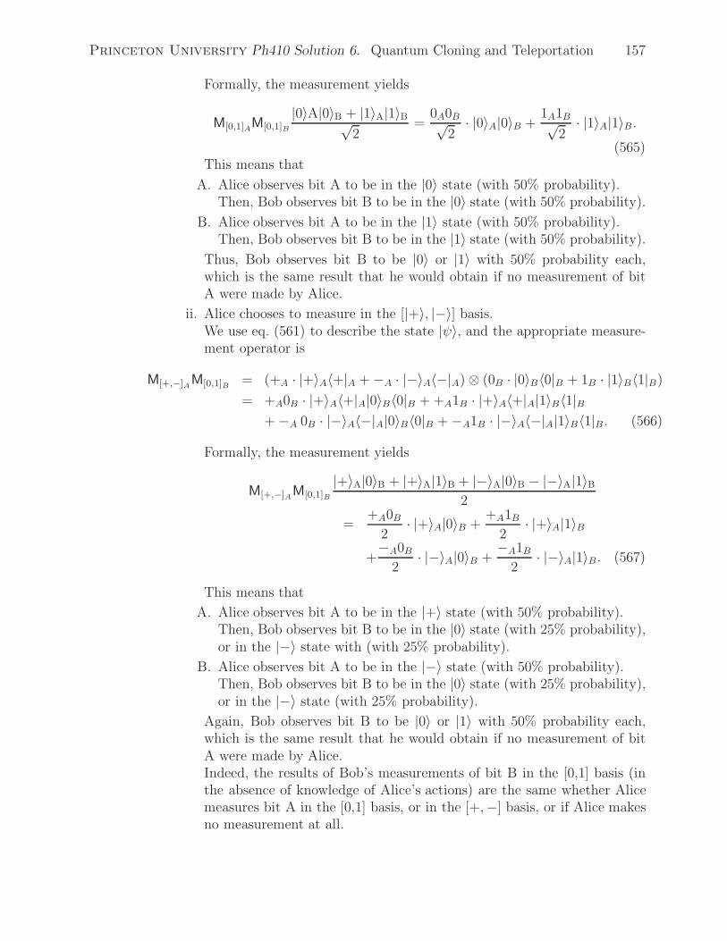
Princeton University Ph410 Solution 6. Quantum Cloning and Teleportation 157
Formally, the measurement yields
M[0,1]AM[0,1]B
|0〉A|0〉B + |1〉A|1〉B√2
=0A0B√
2· |0〉A|0〉B +
1A1B√2
· |1〉A|1〉B .(565)
This means that
A. Alice observes bit A to be in the |0〉 state (with 50% probability).Then, Bob observes bit B to be in the |0〉 state (with 50% probability).
B. Alice observes bit A to be in the |1〉 state (with 50% probability).Then, Bob observes bit B to be in the |1〉 state (with 50% probability).
Thus, Bob observes bit B to be |0〉 or |1〉 with 50% probability each,which is the same result that he would obtain if no measurement of bitA were made by Alice.
ii. Alice chooses to measure in the [|+〉, |−〉] basis.We use eq. (561) to describe the state |ψ〉, and the appropriate measure-ment operator is
M[+,−]AM[0,1]B = (+A · |+〉A〈+|A + −A · |−〉A〈−|A) ⊗ (0B · |0〉B〈0|B + 1B · |1〉B〈1|B)
= +A0B · |+〉A〈+|A|0〉B〈0|B + +A1B · |+〉A〈+|A|1〉B〈1|B+ −A 0B · |−〉A〈−|A|0〉B〈0|B + −A1B · |−〉A〈−|A|1〉B〈1|B . (566)
Formally, the measurement yields
M[+,−]AM[0,1]B
|+〉A|0〉B + |+〉A|1〉B + |−〉A|0〉B − |−〉A|1〉B2
=+A0B
2· |+〉A|0〉B +
+A1B2
· |+〉A|1〉B
+−A0B
2· |−〉A|0〉B +
−A1B2
· |−〉A|1〉B . (567)
This means that
A. Alice observes bit A to be in the |+〉 state (with 50% probability).Then, Bob observes bit B to be in the |0〉 state (with 25% probability),or in the |−〉 state with (with 25% probability).
B. Alice observes bit A to be in the |−〉 state (with 50% probability).Then, Bob observes bit B to be in the |0〉 state (with 25% probability),or in the |−〉 state (with 25% probability).
Again, Bob observes bit B to be |0〉 or |1〉 with 50% probability each,which is the same result that he would obtain if no measurement of bitA were made by Alice.Indeed, the results of Bob’s measurements of bit B in the [0,1] basis (inthe absence of knowledge of Alice’s actions) are the same whether Alicemeasures bit A in the [0,1] basis, or in the [+,−] basis, or if Alice makesno measurement at all.

Princeton University Ph410 Solution 6. Quantum Cloning and Teleportation 158
(b) Bob chooses to measure in the [|+〉, |−〉] basis.
i. Alice chooses to measure in the [|0〉, |1〉] basis.
A. Alice observes bit A to be in the |0〉 state (with 50% probability).Then, Bob observes bit B to be in the |+〉 state (with 25% probability),or in the |−〉 state with (with 25% probability).
B. Alice observes bit A to be in the |1〉 state (with 50% probability).Then, Bob observes bit B to be in the |+〉 state (with 25% probability),or in the |−〉 state (with 25% probability).
ii. Alice chooses to measure in the [|+〉, |−〉] basis.
A. Alice observes bit A to be in the |+〉 state (with 50% probability).Then, Bob observes bit B to be in the |+〉 state (with 50% probability).
B. Alice observes bit A to be in the |−〉 state (with 50% probability).Then, Bob observes bit B to be in the |−〉 state (with 50% probability).
By himself, Bob observes bit B to be |0〉 or |1〉 with equal probability if he measuresin the [|0〉, |1〉] basis, or that bit B is |+〉 or |−〉 with equal probability if hemeasures in the [|+〉, |−〉] basis. This gives him no clue as to what Alice has done;he doesn’t know whether she made measurements in the [|0〉, |1〉] basis or in the[|+〉, |−〉] basis, or whether she made any measurements at all.
In my view, Bob has learned nothing at all about bit A from his measurementsof bit B.141 There is no “signal” from one part of an entangled state to the other.
Suppose, however, that Bob could make lots of copies of bit B, each having theentanglement with bit A given in eq. (558)-(561). Then he could measure halfof the copies in the basis [|0〉, |1〉] and the other half in the basis [|+〉, |−〉]. Ifhe observes the various copies of bit B to be |0〉, |1〉, |+〉 and |−〉 with equalprobability, he can conclude with good assurance that Alice made no measurementof bit A. But if he found no copies of bit B to be one of those four states (e.g.,no |+〉), while half of the copies to be its basis partner (e.g., 50% |−〉), then hecould conclude that Alice had made a measurement in that basis (e.g., [|+〉, |−〉]),and that her result was that bit A is the same state as he found 50% of the time(e.g., |−〉). He could interpret these results as a signal from Alice as to her choiceof basis and of her result of a measurement, despite their measurements beingspacelike-separated. This would imply faster-than-light communication!
So it is happily consistent with our trust in the theory of relativity that the neededcloning of the entangled state (106) cannot be done.142
141However, starting with Einstein, another kind of comment has been made. Namely, that if Bob measuresbit B to be, say |0〉, then he can “predict with certainty” that IF Alice measured bit A in the [|0〉, |1〉] basis,then she would find bit A to be |0〉 also. Similarly, Bob can “predict with certainty” that if he measures bitB to be |+〉, then IF Alice measured bit A in the [|+〉, |−〉] basis she would find bit A to be |+〉 also. Suchconditional predictions are obviously unsatisfactory because they do not contain useful knowledge aboutbit A. Nonetheless, in a very loose usage of words they imply “certain knowledge” simultaneously aboutspacelike-separated quantum states in two different bases, which led Einstein to remark that they impliedsome kind of “spooky” action at a distance, which in turn suggested to him that quantum theory wassomehow “incomplete”. I subscribe to the camp of Bohr that this logic does not warrant such conclusions.http://physics.princeton.edu/~mcdonald/examples/QM/bohr_pr_48_696_35.pdf
142 We don’t need the full no-cloning theorem to conclude that we cannot make an “exact” copy of bit B if
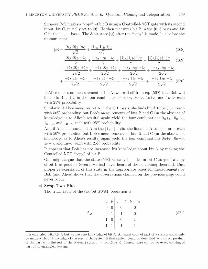
Princeton University Ph410 Solution 6. Quantum Cloning and Teleportation 159
Suppose Bob makes a “copy” of bit B using a Controlled-NOT gate with its secondinput, bit C, initially set to |0〉. He then measures bit B in the [0,1] basis and bitC in the [+,−] basis. The 3-bit state |ψ〉 after the “copy” is made, but before themeasurement, is
|ψ〉=|0〉A|0〉B|0〉C√
2+
|1〉A|1〉B|1〉C√2
(568)
=|0〉A|0〉B|+〉C
2+
|0〉A|0〉B|−〉C2
+|1〉A|1〉B|+〉C
2− |1〉A|1〉B|−〉C
2(569)
=|+〉A|0〉B|+〉C
2√
2+
|−〉A|0〉B|+〉C2√
2+
|+〉A|0〉B|−〉C2√
2+
|−〉A|0〉B|−〉C2√
2
+|+〉A|1〉B|+〉C
2√
2− |−〉A|1〉B|+〉C
2√
2− |+〉A|1〉B|−〉C
2√
2+
|−〉A|1〉B|−〉C2√
2.(570)
If Alice makes no measurement of bit A, we read off from eq. (569) that Bob willfind bits B and C in the four combinations 0B+C, 0B−C, 1B+C, and 1B−C eachwith 25% probability.
Similarly, if Alice measures bit A in the [0,1] basis, she finds bit A to be 0 or 1 eachwith 50% probability, but Bob’s measurements of bits B and C (in the absence ofknowledge as to Alice’s results) again yield the four combinations 0B+C, 0B−C,1B+C, and 1B−C each with 25% probability.
And if Alice measures bit A in the [+,−] basis, she finds bit A to be + or − eachwith 50% probability, but Bob’s measurements of bits B and C (in the absence ofknowledge as to Alice’s results) again yield the four combinations 0B+C, 0B−C,1B+C, and 1B−C each with 25% probability.
It appears that Bob has not increased his knowledge about bit A by making theControlled-NOT “copy” of bit B.
One might argue that the state (568) actually includes in bit C as good a copyof bit B as possible (even if we had never heard of the no-cloning theorem). But,proper re-expression of this state in the appropriate bases for measurements byBob (and Alice) shows that the observations claimed on the previous page couldnever occur.
(c) Swap Two Bits
The truth table of the two-bit SWAP operation is
Sab :
a b a′ = b b′ = a
0 0 0 0
0 1 1 0
1 0 0 1
1 1 1 1
(571)
it is entangled with bit A but we have no knowledge of bit A. An exact copy of part of a system could onlybe made without knowledge of the rest of the system if that system could be described as a direct productof the part with the rest of the system (|system〉 = |part〉|rest〉). Hence, there can be no exact copying ofpart of an entangled system.

Princeton University Ph410 Solution 6. Quantum Cloning and Teleportation 160
Hence, the 4 × 4 matrix for the SWAP operator is
Sab =
⎛⎜⎜⎜⎜⎜⎜⎝
1 0 0 0
0 0 1 0
0 1 0 0
0 0 0 1
⎞⎟⎟⎟⎟⎟⎟⎠. (572)
This matrix is closely related to the matrix (552) for the Controlled-NOT operatorCab.
The hint is to consider the Controlled-NOT operator Cba, whose truth table is
Cba :
a b a′ b′
0 0 0 0
0 1 1 1
1 0 1 0
1 1 0 1
(573)
Hence, the 4 × 4 matrix for the Cba operator is
Cba =
⎛⎜⎜⎜⎜⎜⎜⎝
1 0 0 0
0 0 0 1
0 0 1 0
0 1 0 0
⎞⎟⎟⎟⎟⎟⎟⎠. (574)
If we apply the two Controlled-NOT operators in sequence, we obtain the matrix
CbaCab =
⎛⎜⎜⎜⎜⎜⎜⎝
1 0 0 0
0 0 0 1
0 0 1 0
0 1 0 0
⎞⎟⎟⎟⎟⎟⎟⎠
⎛⎜⎜⎜⎜⎜⎜⎝
1 0 0 0
0 1 0 0
0 0 0 1
0 0 1 0
⎞⎟⎟⎟⎟⎟⎟⎠
=
⎛⎜⎜⎜⎜⎜⎜⎝
1 0 0 0
0 0 1 0
0 0 0 1
0 1 0 0
⎞⎟⎟⎟⎟⎟⎟⎠. (575)
This is not yet eq. (572), but we persevere and multiply eq. (575) by Cab,
CabCbaCab =
⎛⎜⎜⎜⎜⎜⎜⎝
1 0 0 0
0 1 0 0
0 0 0 1
0 0 1 0
⎞⎟⎟⎟⎟⎟⎟⎠
⎛⎜⎜⎜⎜⎜⎜⎝
1 0 0 0
0 0 1 0
0 0 0 1
0 1 0 0
⎞⎟⎟⎟⎟⎟⎟⎠
=
⎛⎜⎜⎜⎜⎜⎜⎝
1 0 0 0
0 0 1 0
0 1 0 0
0 0 0 1
⎞⎟⎟⎟⎟⎟⎟⎠
= Sab. (576)
Likewise, CbaCabCba = Sab.
A diagram for a SWAP circuit is
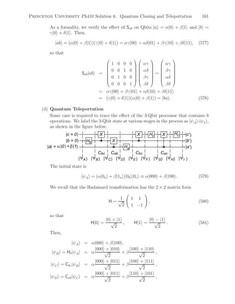
Princeton University Ph410 Solution 6. Quantum Cloning and Teleportation 161
As a formality, we verify the effect of Sab on Qbits |a〉 = α|0〉 + β|1〉 and |b〉 =γ|0〉 + δ|1〉. Then,
|ab〉 = (α|0〉 + β|1〉)(γ|0〉 + δ|1〉) = αγ|00〉 + αδ|01〉 + βγ|10〉 + βδ|11〉, (577)
so that
Sab|ab〉 =
⎛⎜⎜⎜⎜⎜⎜⎝
1 0 0 0
0 0 1 0
0 1 0 0
0 0 0 1
⎞⎟⎟⎟⎟⎟⎟⎠
⎛⎜⎜⎜⎜⎜⎜⎝
αγ
αδ
βγ
βδ
⎞⎟⎟⎟⎟⎟⎟⎠
=
⎛⎜⎜⎜⎜⎜⎜⎝
αγ
βγ
αδ
βδ
⎞⎟⎟⎟⎟⎟⎟⎠
= αγ|00〉 + βγ|01〉 + αδ|10〉 + βδ|11〉= (γ|0〉 + δ|1〉)(α|0〉 + β|1〉) = |ba〉. (578)
(d) Quantum Teleportation
Some care is required to trace the effect of the 3-Qbit processor that contains 8operations. We label the 3-Qbit state at various stages in the process as |ψA〉-|ψI〉,as shown in the figure below.
The initial state is
|ψA〉 = (α|0a〉 + β|1a〉)|0b〉|0c〉 ≡ α|000〉 + β|100〉. (579)
We recall that the Hadamard transformation has the 2 × 2 matrix form
H =1√2
⎛⎝ 1 1
1 −1
⎞⎠ , (580)
so that
H|0〉 =|0〉 + |1〉√
2, H|1〉 =
|0〉 − |1〉√2
. (581)
Then,
|ψA〉 = α|000〉 + β|100〉,|ψB〉 = Hb|ψA〉 = α
|000〉 + |010〉√2
+ β|100〉 + |110〉√
2,
|ψC〉 = Cbc|ψB〉 = α|000〉 + |011〉√
2+ β
|100〉 + |111〉√2
,
|ψD〉 = Cab|ψC〉 = α|000〉 + |011〉√
2+ β
|110〉 + |101〉√2
,

Princeton University Ph410 Solution 6. Quantum Cloning and Teleportation 162
|ψE〉 = Ha|ψD〉 = α|000〉 + |100〉 + |011〉 + |111〉
2+ β
|010〉 − |110〉 + |001〉 − |101〉2
,
|ψF 〉 = Cbc|ψE〉 = α|000〉 + |100〉 + |010〉 + |110〉
2+ β
|011〉 − |111〉 + |001〉 − |101〉2
,
|ψG〉 = Hc|ψF 〉 = α|000〉 + |001〉 + |100〉 + |101〉 + |010〉 + |011〉 + |110〉 + |111〉
2√
2
+β|010〉 − |011〉 − |110〉 + |111〉 + |000〉 − |001〉 − |100〉 + |101〉
2√
2,
|ψH〉 = Cac|ψG〉 = α|000〉 + |001〉 + |101〉 + |100〉 + |010〉 + |011〉 + |111〉 + |110〉
2√
2
+β|010〉 − |011〉 − |111〉 + |110〉 + |000〉 − |001〉 − |101〉 + |100〉
2√
2,
|ψI〉 = Hc|ψH〉 = α|000〉 + |001〉 + |000〉 − |001〉 + |100〉 − |101〉 + |100〉 + |101〉
4
+α|010〉 + |011〉 + |010〉 − |011〉 + |110〉 − |111〉 + |110〉 + |111〉
4
+β|010〉 + |011〉 − |010〉 + |011〉 − |110〉 + |111〉 + |110〉 + |111〉
4
+β|000〉 + |001〉 − |000〉 + |001〉 − |100〉 + |101〉 + |100〉 + |101〉
4
= α|000〉 + |100〉 + |010〉 + |110〉
2+ β
|011〉 + |111〉 + |001〉 + |101〉2
= α|0〉 + |1〉√
2
|0〉 + |1〉√2
|0〉 + β|0〉 + |1〉√
2
|0〉 + |1〉√2
|1〉
=|0a〉 + |1a〉√
2
|0b〉 + |1b〉√2
(α|0c〉 + β|1c〉). (582)
Despite the entangling effects of the Hadamard operations, the final state |ψI〉 =|a′〉|b′〉|c′〉 is a direct product state in which |c′〉 is the same as the initial state|a〉. The final states |a′〉 and |b′〉 could, if desired, be brought to |0〉 states withadditional operations Ha and Hb.
Turning to the version of the above process in which Alice and Bob split thingsup, we see that Alice measures bits a and b when the system has state |ψE〉. Thereare 4 possible outcomes of her measurements, resulting in one of four states,
|ψE00〉 = |00〉(α|0〉 + β|1〉), (583)
|ψE01〉 = |01〉(α|1〉 + β|0〉), (584)
|ψE10〉 = |10〉(α|0〉 − β|1〉), (585)
|ψE11〉 = |11〉(α|1〉 − β|0〉). (586)
We see that if Alice’s measurements of bits a and b are |00〉, Bob doesn’t actuallyhave to do anything to bit c; it already is in the unknown state α|0〉+β|1〉. This isperhaps the source of the description teleportation. It seems as if Alice’s measure-ment transferred information from bit a to bit c without any obvious interaction
Princeton University Ph410 Solution 6. Quantum Cloning and Teleportation 163
between them, and over the possibly large distance between the location of thesebits. Since we can’t identify a classical mechanism for this, we might declare thistransfer to be “instantaneous”, and hence a kind of “teleportation”.
But, Bob can’t really know that his bit c has taken on the initial state of bit auntil the classical information about the measurements of bits a and c has arrived.So in practice, there is no faster-than-light transfer of knowledge. However, thisquantum process remains somewhat surprising, even mysterious from a classicalpoint of view.
For completeness, we should verify that the 4 transformations of Bob, Cbc, Hc, Cacand finally Hc again, always result in bit c ending up as α|0〉 + β|1〉. Perhaps itsuffices to do this for only the cases where the measurements of bits a and b are|00〉 and |11〉.|ψF00
〉 = Cbc|ψE00〉 = |00〉(α|0〉 + β|1〉),
|ψG00〉 = Hc|ψF00
〉 = |00〉(α|0〉 + |1〉√
2+ β
|0〉 − |1〉√2
),
|ψH00〉 = Cac|ψG00
〉 = |00〉(α|0〉 + |1〉√
2+ β
|0〉 − |1〉√2
),
|ψI00〉 = Hc|ψH00〉 = |00〉
(α|0〉 + |1〉 + |0〉 − |1〉
2+ β
|0〉 + |1〉 − |0〉 + |1〉√2
),
= |00〉(α|0〉 + β|1〉). (587)
Similarly,
|ψF11〉 = Cbc|ψE11
〉 = |11〉(α|0〉 − β|1〉),|ψG11
〉 = Hc|ψF11〉 = |11〉
(α|0〉 + |1〉√
2− β
|0〉 − |1〉√2
),
|ψH11〉 = Cac|ψG11
〉 = |11〉(α|0〉 + |1〉√
2+ β
|0〉 − |1〉√2
),
|ψI11〉 = Hc|ψH11〉 = |11〉
(α−|0〉 − |1〉 + |0〉 − |1〉
2+ β
|0〉 + |1〉 − |0〉 + |1〉√2
),
= |11〉(α|0〉 + β|1〉). (588)
The result that it makes no difference to the outcome of the final 4 transformationswhether bits a and b are measured at the beginning or the end arises because thosebits only serve as control bits in Controlled-NOT operations. Indeed, for anyControlled-U gate (where U is any 1-Qbit unitary transformation), if the controlQbit is to be measured in the [0,1] basis then the measurement may be performedeither before or after the gate is executed, without making any difference to thefinal outcome.143
From the last line of eq. (582), we see that if Alice did not measure bits |a〉 andb, and Bob performed Hadamard transformation Ha on the state |ψI〉, the result
143 http://physics.princeton.edu/~mcdonald/examples/QM/griffiths_prl_76_3228_96.pdf

Princeton University Ph410 Solution 6. Quantum Cloning and Teleportation 164
would be
|ψJ〉 = Ha|ψI〉 = |0a〉|0b〉 + |1b〉√2
(α|0c〉 + β|1c〉), (589)
since Ha|aI〉 = Ha|+a〉 = |0a〉. A lesson is that the Controlled-NOT operationswith |a〉 as the control bit entangle this Qbit with bits |b〉 and |c〉, such that thecoefficients α and β in the initial state of |a〉 are no longer an exclusive propertyof that bit, but are shared with the other bits. Rather, in the final state |ψI〉these coefficients are now associated with bit |c′〉, and not with |a′〉, which latterbit is in the state |+a〉 independent of α and β.
The “delocalization” of the properties of a Qbit via entangling it with anotherQbit will be exploited in other quantum computations discussed later in thiscourse.
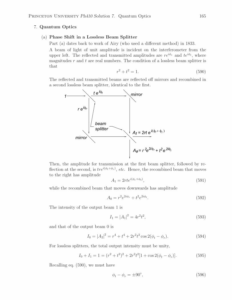
Princeton University Ph410 Solution 7. Quantum Optics 165
7. Quantum Optics
(a) Phase Shift in a Lossless Beam Splitter
Part (a) dates back to work of Airy (who used a different method) in 1833.
A beam of light of unit amplitude is incident on the interferometer from theupper left. The reflected and transmitted amplitudes are reiφr and teiφt , wheremagnitudes r and t are real numbers. The condition of a lossless beam splitter isthat
r2 + t2 = 1. (590)
The reflected and transmitted beams are reflected off mirrors and recombined ina second lossless beam splitter, identical to the first.
Then, the amplitude for transmission at the first beam splitter, followed by re-flection at the second, is trei(φt+φr), etc. Hence, the recombined beam that movesto the right has amplitude
A1 = 2rtei(φr+φt), (591)
while the recombined beam that moves downwards has amplitude
A0 = r2e2iφr + t2e2iφt . (592)
The intensity of the output beam 1 is
I1 = |A1|2 = 4r2t2, (593)
and that of the output beam 0 is
I0 = |A2|2 = r4 + t4 + 2r2t2 cos 2(φt − φr). (594)
For lossless splitters, the total output intensity must be unity,
I0 + I1 = 1 = (r2 + t2)2 + 2r2t2[1 + cos 2(φt − φr)]. (595)
Recalling eq. (590), we must have
φt − φr = ±90◦, (596)

Princeton University Ph410 Solution 7. Quantum Optics 166
for any value of the splitting ratio r2 : t2.
Via additional arguments we can show that144
φt − φr = −90◦, i .e., φr = φt +π
2, and eiφr = ieiφt . (597)
We will use this form in parts (c)-(e).
Note that eqs. (594) and (596) imply that the intensity of output beam 0 is
I0 = r4 + t4 − 2r2t2 = (r2 − t2)2, (598)
so that for an interferometer with 50:50 beam splitters, no light would emerge onoutput path 0.
(b) Bunching of Photons in a Beam Splitter
Part (b) appears to have been first considered by Hong et al. in 1987.145 Seealso.146
In a lossless beam splitter the amplitudes for a single photon to be reflected ortransmitted have magnitudes r =
√R and t =
√T , where R and T are the
probability that a single photon is reflected or transmitted, respectively. For a50:50 splitter, we have r = t = 1/
√2. If two photons appear after the beam
splitter on the same side (and none on the other), then one of these was reflectedand one was transmitted. The amplitude for this is therefore
A2,0 = A0,2 ∝ reiφrteiφt . (599)
In this case both photons end up in the same final state. Since photons are bosons,the amplitude for having multiple particles in the same final state is enhanced bythe square root of the number of ways the particles can be rearranged. Since the“first” output photon could be either the first or the second input photon, theenhancement factor is
√2. That is,
A2,0 = A0,2 =√
2reiφr teiφt . (600)
so the probability that two output photons appear on the same side of the splitteris
P2,0 = P0,2 = |A2,0|2 = 2r2t2 = 2RT. (601)
For a 50:50 splitter,
P2,0 = P0,2 =1
2(50:50 splitter). (602)
One output photon could appear on each side of beam splitter in either of twoways: both input photons are reflected, or both are transmitted. The amplitudefor this is
A1,1 = reiφrreiφr + teiφtteiφt , (603)
144See, for example, problem 4(b) ofhttp://physics.princeton.edu/~mcdonald/examples/ph501set6.pdf
145 http://physics.princeton.edu/~mcdonald/examples/QM/hong_prl_59_2044_87.pdf146 http://physics.princeton.edu/~mcdonald/examples/QM/campos_pra_40_1371_89.pdf
Princeton University Ph410 Solution 7. Quantum Optics 167
so the probability that one output photon appears on each side of the splitter is
P1,1 = |A1|2 = r4 + t4 + 2r2t2 cos[2(φr − φt)] = r4 + t4 − 2r2t2 = (R− T )2, (604)
using eq. (596). For a 50:50 splitter, we obtain the possibly surprising result that
P1,1 = 0 (50:50 splitter); (605)
i.e., a quantum analysis predicts that the case of one photon emerging from eachside of the splitter does not occur.
Note that in general
P2,0 + P1,1 + P0,2 = (R − T )2 + 2RT = (R + T )2 = 1, (606)
so that the total probability is indeed unity.
In contrast, a classical analysis for input beams of intensities i1 and i2 is that theamplitudes of the two (in-phase) input beams are a1 =
√i1 and a2 =
√i2. The
output beam 1 (in the direction of the input beam 1) is due to transmission ofinput beam 1 and reflection of input beam 2, and so has amplitude
A1 = a1teiφt + a2re
iφr . (607)
Similarly, the classical amplitude for output beam 2 is
A2 = a1reiφr + a2te
iφt . (608)
The intensities of the output beams are therefore
I1 = |A1|2 = i1T + i2R+ 2√
i1i2rt cos(φr − φt) = i1T + i2R, (609)
andI2 = |A2|2 = i1R+ i2T + 2
√i1i2rt cos(φr − φt) = i1R+ i2T. (610)
When R = T = 1/2, we find that I1 = I2 = (i1 + i2)/2. Thus, the classicalexpectation is that a 50:50 beam splitter just splits the beams 50:50 no matterwhat direction they come from and what intensities they have.
But the quantum result for the case of only one photon in each input “beam” isthat there is zero probability of (1 + 1)/2 = 1 photon in an output beam. Rather,the photons “bunch” into a single output beam on only one side of a lossless 50:50splitter.147
(c) A Beam Splitter as a Quantum Processor
Part (c) was perhaps first considered by Yurke et al. in 1986.148
The transmission coefficient of the lossless beam splitter can be written as T =1 − R = cos2 β
2, since we have R = sin2 β
2. The magnitudes of the reflected and
transmitted amplitudes are then r = sin β2
and t = cos β2.
147 The quantum result for input beams of arbitrary numbers of photons is discussed inhttp://physics.princeton.edu/~mcdonald/examples/bunching.pdf
148 http://physics.princeton.edu/~mcdonald/examples/QM/yurke_pra_33_4033_86.pdf

Princeton University Ph410 Solution 7. Quantum Optics 168
We define, without loss of generality, the phase shift of a transmitted photon to beφt = 0. Then from eq. (597) we have that the phase shift of a reflected photon isφr = π/2. Hence, the beam splitter takes a photon |0〉 into cos β
2|0′〉+eiπ/2 sin β
2|1′〉.
Similarly, the beam splitter takes the input state |1〉 into (eiπ/2 sin β2|0′〉+cos β
2|1′〉.
Therefore, we can write the action of the beam splitter as the 2×2 unitary matrix
M =
⎛⎝ cos β
2eiπ/2 sin β
2
eiπ/2 sin β2
cos β2
⎞⎠ . (611)
To understand the effect of a dielectric plate on the propagation of a photon, werecall that a photon of wavelength λ that travels in vacuum along the z directionhas wave function
ψvacuum = ei(kz−ωt), (612)
where k = 2π/λ is the (free-space) wave number and ω = kc is the angularfrequency of the photon. Of course, c is the speed of light in vacuum. When thisphoton is inside a dielectric medium its speed is reduced to v = c/n, where n isthe index of refraction. The angular frequency of the photon is unchanged, so thewave number becomes k′ = ω/v = ωn/c = kn. The wave function of the photoninside the dielectric is therefore
ψdielectric = ei(k′z−ωt) = ei(knz−ωt). (613)
If the dielectric plate extends from z = 0 to d, then the wave function of thephoton at the exit of the plate is
ψ(z = d) = ei(knd−ωt) = ei(kd−ωt+k(n−1)d) = ei(kd−ωt+φ), (614)
where
φ = k(n − 1)d) =2πd(n − 1)
λ(615)
is the phase difference between the photon that has traversed the dielectric plateand a photon that traveled distance d in vacuum.
Hence, the addition of the four wave-shifting plates to the beam splitter, as shownin the figure below, has the effect that
|0〉 → cosβ
2ei(φa+φc)|0′〉 + sin
β
2ei(φa+φd+π/2)|1′〉,
|1〉 → sinβ
2ei(φb+φc+π/2)|0′〉 + cos
β
2ei(φb+φd)|1′〉. (616)
Expressing this transformation as a 2 × 2 unitary matrix U, we have
U =
⎛⎝ cos β
2ei(φa+φc) sin β
2ei(φb+φc+π/2)
sin β2ei(φa+φd+π/2) cos β
2ei(φb+φd)
⎞⎠ . (617)

Princeton University Ph410 Solution 7. Quantum Optics 169
The form (617) is similar to the general form of a 2 × 2 unitary matrix given byeqs. (44) and (56),
U = eiδ
⎛⎝ cos β
2ei(α+γ)/2 sin β
2ei(−α+γ)/2
− sin β2ei(α−γ)/2) cos β
2e−i(α+γ)/2
⎞⎠ . (618)
Indeed, the two forms (617) and (618) will be identical when
φa + φc =α
2+γ
2+ δ, (619)
φb + φc = −α2
+γ
2+ δ − π
2, (620)
φa + φd =α
2− γ
2+ δ +
π
2, (621)
φb + φd = −α2− γ
2+ δ. (622)
Since, for example (622) = (620) + (621) - (619), we have only 3 relations amongthe 4 phases φa, φb, φc and φd. We can then, for instance, set any one of these 4phases to 0 and still obtain a solution to eqs. (619)-(622). Thus,
φa = 0, φb = −α− π
2, φc =
α
2+γ
2+ δ, φd =
α
2− γ
2+ δ+
π
2. (623)
permits a beam splitter (with R = sin2 β2) + 3 wave-shifter plates to represent an
arbitrary 2 × 2 unitary transformation.
The gate
Z =
⎛⎝ 1 0
0 −1
⎞⎠ . (624)
does nothing to |0〉 and changes the phase of |1〉 by π. Hence, we expect that wecan implement an optical Z gate with no beam splitter, phase shifts φa = φc = 0on the path of |0〉, and phase shifts φb + φd = π on the path of |1〉.Comparing eq. (624) to the general form (618), we quickly see that
α = −π, β = 0, γ = 0, δ =π
2. (625)
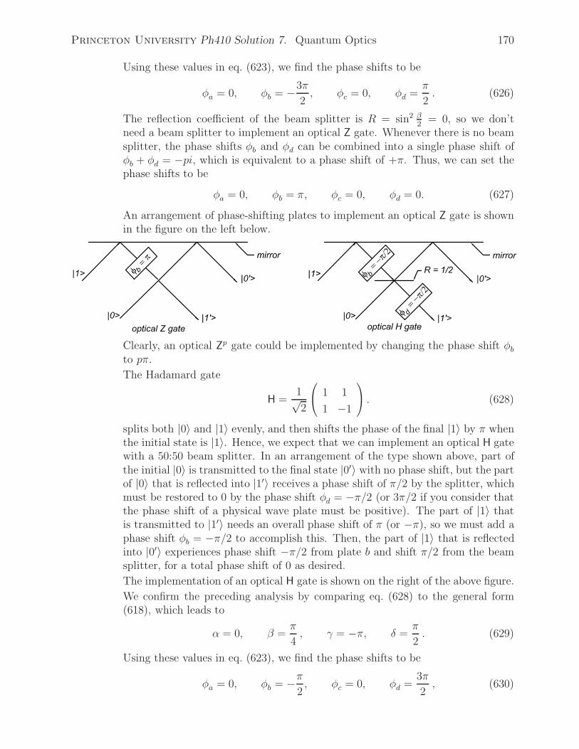
Princeton University Ph410 Solution 7. Quantum Optics 170
Using these values in eq. (623), we find the phase shifts to be
φa = 0, φb = −3π
2, φc = 0, φd =
π
2. (626)
The reflection coefficient of the beam splitter is R = sin2 β2
= 0, so we don’tneed a beam splitter to implement an optical Z gate. Whenever there is no beamsplitter, the phase shifts φb and φd can be combined into a single phase shift ofφb + φd = −pi, which is equivalent to a phase shift of +π. Thus, we can set thephase shifts to be
φa = 0, φb = π, φc = 0, φd = 0. (627)
An arrangement of phase-shifting plates to implement an optical Z gate is shownin the figure on the left below.
Clearly, an optical Zp gate could be implemented by changing the phase shift φbto pπ.
The Hadamard gate
H =1√2
⎛⎝ 1 1
1 −1
⎞⎠ . (628)
splits both |0〉 and |1〉 evenly, and then shifts the phase of the final |1〉 by π whenthe initial state is |1〉. Hence, we expect that we can implement an optical H gatewith a 50:50 beam splitter. In an arrangement of the type shown above, part ofthe initial |0〉 is transmitted to the final state |0′〉 with no phase shift, but the partof |0〉 that is reflected into |1′〉 receives a phase shift of π/2 by the splitter, whichmust be restored to 0 by the phase shift φd = −π/2 (or 3π/2 if you consider thatthe phase shift of a physical wave plate must be positive). The part of |1〉 thatis transmitted to |1′〉 needs an overall phase shift of π (or −π), so we must add aphase shift φb = −π/2 to accomplish this. Then, the part of |1〉 that is reflectedinto |0′〉 experiences phase shift −π/2 from plate b and shift π/2 from the beamsplitter, for a total phase shift of 0 as desired.
The implementation of an optical H gate is shown on the right of the above figure.
We confirm the preceding analysis by comparing eq. (628) to the general form(618), which leads to
α = 0, β =π
4, γ = −π, δ =
π
2. (629)
Using these values in eq. (623), we find the phase shifts to be
φa = 0, φb = −π2, φc = 0, φd =
3π
2, (630)
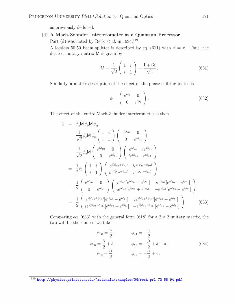
Princeton University Ph410 Solution 7. Quantum Optics 171
as previously deduced.
(d) A Mach-Zehnder Interferometer as a Quantum Processor
Part (d) was noted by Reck et al. in 1994.149
A lossless 50:50 beam splitter is described by eq. (611) with β = π. Thus, thedesired unitary matrix M is given by
M =1√2
⎛⎝ 1 i
i 1
⎞⎠ =
I + iX√2
. (631)
Similarly, a matrix description of the effect of the phase shifting plates is
φ =
⎛⎝ eiφ0 0
0 eiφ1
⎞⎠ . (632)
The effect of the entire Mach-Zehnder interferometer is then
U = φcMφbMφa
=1√2φcMφb
⎛⎝ 1 i
i 1
⎞⎠⎛⎝ eiφa0 0
0 eiφa1
⎞⎠
=1√2φcM
⎛⎝ eiφb0 0
0 eiφb1
⎞⎠⎛⎝ eiφa0 ieiφa1
ieiφa0 eiφa1
⎞⎠
=1
2φc
⎛⎝ 1 i
i 1
⎞⎠⎛⎝ ei(φa0+φb0) iei(φa1+φb0)
iei(φa0+φb1) ei(φa1+φb1)
⎞⎠
=1
2
⎛⎝ eiφc0 0
0 eiφc1
⎞⎠⎛⎝ eiφa0[eiφb0 − eiφb1] ieiφa1[eiφb0 + eiφb1]
ieiφa0[eiφb0 + eiφb1] −eiφa1[eiφb0 − eiφb1]
⎞⎠
=1
2
⎛⎝ ei(φa0+φc0)[eiφb0 − eiφb1] iei(φa1+φc0)[eiφb0 + eiφb1]
iei(φa0+φc1)[eiφb0 + eiφb1] −ei(φa1+φc1)[eiφb0 − eiφb1]
⎞⎠ . (633)
Comparing eq. (633) with the general form (618) for a 2 × 2 unitary matrix, thetwo will be the same if we take
φa0 =γ
2, φa1 = −γ
2,
φb0 =β
2+ δ, φb1 = −β
2+ δ + π, (634)
φc0 =α
2, φc1 = −α
2+ π.
149 http://physics.princeton.edu/~mcdonald/examples/QM/reck_prl_73_58_94.pdf

Princeton University Ph410 Solution 7. Quantum Optics 172
(e) An Optical Controlled-NOT Gate
N -Qbit gates based on only a single photon were discussed by Reck et al.150 Two-Qbit gates based on 2 photons have been discussed by Koashi et al.,151 by Knillet al.,152 and by O’Brien et al.153 A variant on this part using polarized photonshas been discussed by Ralph et al.154
When the only photon incident on the interferometer is |0y〉, then the amplitudesfor the various splittings are shown in the figure below.
In this case we never want a photon to emerge as |1′y〉, which requires that irarcrd =itarbtd. The simplest solution to this is, recalling that r2 + t2 = 1,
ra = ta =1√2, rb = rc, rd = tb =
1√2. (635)
The probability that a photon in initial state |0y〉 emerges as |0′y〉 is then r2b = Rb.
The probability that the photon emerges at the unused output port is r2at
2c = t2b/2,
and the probability that the photon emerges at the output port labeled |1′x〉 ist2at
2b = t2b/2. Thus, the total probability for the final states is r2
b + 2(t2b/2) = 1, asexpected.
When the only photon incident on the interferometer is |1y〉, then the amplitudesfor the various splittings are shown in the figure on the next page.
150 http://physics.princeton.edu/~mcdonald/examples/QM/reck_prl_73_58_94.pdf151 http://physics.princeton.edu/~mcdonald/examples/QM/koashi_pra_63_030301_01.pdf152 http://physics.princeton.edu/~mcdonald/examples/QM/knill_nature_409_46_01.pdf153 http://physics.princeton.edu/~mcdonald/examples/QM/obrien_nature_426_264_03.pdf154 http://physics.princeton.edu/~mcdonald/examples/QM/ralph_pra_65_024308_02.pdf

Princeton University Ph410 Solution 7. Quantum Optics 173
In this case we never want a photon to emerge as |0′y〉, which requires that rarbrd =tarctd. A solution to this is again eq. (635). The probability that |1y〉 emerges as|1′y〉 is r2
b = Rb.
Turning now to the case when the “control” photon is in the state |1x〉 and the“target” photon is in the state |0y〉, the splittings are shown in the figure below.To organize the bookkeeping, we label the 4 output ports as I, II, III and IV.
One photon is incident on each side of splitter b, and we desire that one photonemerge from each side. Recalling eq. (603), with φt = 0 and φr = π/2, theamplitude that one photon emerges from each side of splitter b is t2b−r2
b times theproduct of the incident amplitudes. Hence, splitter b cannot be a 50:50 device.
We desire that one photon emerges from port I (in state |1′x〉) and the other photonemerges from port III (in state |1′y〉) and not from port II (in state |0′y〉).

Princeton University Ph410 Solution 7. Quantum Optics 174
There are two ways that one photon could emerge from port I and one from portII:
i. One travels on path |0y〉-a-c-d-II and the other on path |1x〉-b-I. The combinedamplitude for this option is (−rarctd)(irb) = −ir2
b/2, recalling that ra = ta =rd = td = 1/
√2 and rb = rc.
ii. The two photons impinge on splitter b, then one goes to port I and the othergoes down to splitter d and into port II. The combined amplitude for thisoption is (ta)(t
2b − r2
b )(ird) = i(1 − 2r2b )/
√2.
We desire that the sum of these two amplitudes be 0,
r2b − (1 − 2r2
b ) = 0, (636)
which requires that r2b = 1/3.
The desired reflection coefficients are therefore
Ra =1
2, Rb =
1
3, Rc =
1
3, Rd =
1
2. (637)
As a check, we verify that the sum of all possible outcomes is unity.
Among the possible fates of the 2 input photons is the case that both photonstravel on the path from splitter b to splitter d. We then need to know the am-plitudes that these 2 photons both emerge in port II, or both in port III, or 1in port II and 1 in port III. If the photons were distinguishable, the amplitudethat both are reflected to port II would be (ird)
2, the amplitude that both aretransmitted to port III would be t2d, and the amplitude that one is transmittedto port II and one is reflected to port III would be irdtd. However, photons arebosons, so the fact that there are two ways to arrange that one is transmitted andone is reflected means that the probability for this is twice that mentioned above,and the amplitude is
√2 times as large: the amplitude that one is transmitted to
port II and one is reflected to port III is actually i√
2rdtd.
We now list the amplitudes for all possible trajectories for the two photons:
A(1 in I, 1 in II) = (−rarctd)(irb) + (ta)(t2b − r2
b )(ird) = 0,
A(1 in I, 1 in III) = (irarcrd)(irb) + (ta)(t2b − r2
b )(td),
A(1 in I, 1 in IV) = (iratc)(irb),
A(1 in II, 1 in III) = (−rarc)(tb)(t2d − r2d) + (ta)(i
√2rbtb)(i
√2rdtd),
A(1 in II, 1 in IV) = (iratc)(itbrd), (638)
A(1 in III, 1 in IV) = (iratc)(tbtd),
A(2 in I) = (ta)(i√
2rbtb).
A(2 in II) = (−rarc)(tb)(i√
2rdtd) + (ta)(i√
2rbtb)(ird)2,
A(2 in III) = (−rarc)(tb)(i√
2rdtd) + (ta)(i√
2rbtb)(td)2 = 0.
The corresponding probabilities are, recalling that r2a = t2a = r2
d = t2d = 1/2,r2b = r2
c = 1/3, t2b = t2c = 2/3:

Princeton University Ph410 Solution 7. Quantum Optics 175
P (1 in I, 1 in II) = 0,
P (1 in I, 1 in III) = r2at
4bt
2d =
4
36,
P (1 in I, 1 in IV) = r2ar
2b t
2c =
4
36,
P (1 in II, 1 in III) = 4t2ar2b t
2br
2dt
2d =
4
36,
P (1 in II, 1 in IV) = r2at
2bt
2cr
2d =
4
36, (639)
P (1 in III, 1 in IV) = r2at
2bt
2ct
2d =
4
36,
P (2 in I) = 2t2ar2b t
2b =
8
36.
P (2 in II) = 8r6ar
2b t
2b =
8
36,
P (2 in III) = 0.
The sum of the probabilities is 1, as expected.
The probability that this configuration behaved like the Controlled-NOT opera-tion |1x0y〉 → |1x1y〉 is only 4/36 = 1/9.
Finally, we examine the case when the “control” photon is in the state |1x〉 andthe “target” photon is in the state |1y〉 with the aid of the figure below.
A(1 in I, 1 in II) = (itarctd)(irb) + (ira)(t2b − r2
b )(ird)
= −r2at
2b = −1
3,
A(1 in I, 1 in III) = (−tarcrd)(irb) + (ira)(t2b − r2
b )(td)
= irata(1 − 3r2b ) = 0. (640)
Thus, P (|1x1y〉 → |1′x1′y〉) = 0 as desired, and P (|1x1y〉 → |1′x0′y〉) = P (|1x0y〉 →|1′x1′y〉) = 1/9.

Princeton University Ph410 Solution 7. Quantum Optics 176
It appears that an optical Controlled-NOT gate that succeeds 1/6 of the time hasnow been demonstrated, although the authors don’t actually mention this:http://physics.princeton.edu/~mcdonald/examples/QM/pryde_prl_92_190402_04.pdf

Princeton University Ph410 Solution 8. Programmable Quantum Computer 177
8. A Programmable Quantum Computer?
This problem is based on a paper by Nielsen and Chuang,155 who do not require thatthe program register be unchanged by operation V.156
Given two 2n×2n unitary matrices Up and Uq, their associated m-Qbit program registerstates |p〉 and |q〉, and the (m + n) × (m + n) unitary matrix V which implements aprogrammable quantum gate array such that
V[|p〉 ⊗ |d〉] = |p〉 ⊗ Up|d〉, (111)
V[|q〉 ⊗ |d〉] = |q〉 ⊗ Uq |d〉, (112)
we take the scalar product of eqs. (111) and (112) to find
[〈p| ⊗ 〈d|]V†V[|q〉 ⊗ |d〉] = [〈p| ⊗ 〈d|][|q〉 ⊗ |d〉] = 〈p|q〉= [〈p| ⊗ 〈d|U†
p][|q〉 ⊗ Uq|d〉] = 〈p|q〉〈d|U†pUq|d〉, (643)
for all n-bit words |d〉.If Up is distinct from Uq then 〈d|U†
pUq|d〉 cannot be 1 for all Qbits |d〉, so in this casewe must have 〈p|q〉 = 0; i.e., the program-register words |p〉 and |q〉 are orthogonalwhenever Up and Uq are distinct.
155 http://physics.princeton.edu/~mcdonald/examples/QM/nielsen_prl_79_321_97.pdf156 This requirement simplifies the analysis, and could always be enforced since the action of V on the
program register |p〉 is a direct product with the action of V on the data register |d〉. That is, we can write
V[|p〉⊗ |d〉] = Vp|p〉 ⊗ Up|d〉, (641)
where Vp is a unitary transformation. If Vp is not the unit matrix, we could define V′ = V−1p ⊗ V. Then,
V′[|p〉 ⊗ |d〉] = |p〉 ⊗ Up|d〉. (642)

Princeton University Ph410 Solution 9. Designer Hamiltonians 178
9. Designer Hamiltonians
(a) The Controlled-NOT operator Cab has the matrix form
Cab =
⎛⎜⎜⎜⎜⎜⎜⎝
1 0 0 0
0 1 0 0
0 0 0 1
0 0 1 0
⎞⎟⎟⎟⎟⎟⎟⎠
=
⎛⎝ I 0
0 X
⎞⎠ (644)
If matrix A acts on bit |a〉 = a0|0〉a + a1|1〉a, and matrix B acts on bit |b〉 =b0|0〉b + b1|1〉b, where we write
A =
⎛⎝ A00 A01
A10 A11
⎞⎠ , and B =
⎛⎝ B00 B01
B10 B11
⎞⎠ , (645)
The the operator tensor product A ⊗ B acts on the bit tensor product |a〉 ⊗ |b〉according to
(A ⊗ B)(|a〉 ⊗ |b〉) = (A|a〉) ⊗ (B|b〉)
=
⎛⎝ A00 A01
A10 A11
⎞⎠⎛⎝ a0
a1
⎞⎠⊗
⎛⎝ B00 B01
B10 B11
⎞⎠⎛⎝ b0
b1
⎞⎠
=
⎛⎝ A00a0 + A01a1
A10a0 + A11a1
⎞⎠ ⊗
⎛⎝ B00b0 +B01b1
B10b0 +B11b1
⎞⎠
=
⎛⎜⎜⎜⎜⎜⎜⎝
A00B00a0b0 + A00B01a0b1 + A10B00a1b0 + A10B10a1b1
A00B10a0b0 + A00B11a0b1 + A10B10a1b0 + A10B11a1b1
A10B00a0b0 + A10B01a0b1 + A11B00a1b0 + A11B10a1b1
A10B10a0b0 + A10B11a0b1 + A11B10a1b0 + A11B11a1b1
⎞⎟⎟⎟⎟⎟⎟⎠
=
⎛⎜⎜⎜⎜⎜⎜⎝
A00B00 A00B01 A10B00 A10B10
A00B10 A00B11 A10B10 A10B11
A10B00 A10B01 A11B00 A11B10
A10B10 A10B11 A11B10 A11B11
⎞⎟⎟⎟⎟⎟⎟⎠
⎛⎜⎜⎜⎜⎜⎜⎝
a0b0
a0b1
a1b0
a1b1
⎞⎟⎟⎟⎟⎟⎟⎠. (646)
Thus,
A ⊗ B =
⎛⎝ A00B A01B
A10B A11B
⎞⎠ . (647)
The result (647) suggests that we write
Cab =
⎛⎝ I 0
0 0
⎞⎠ +
⎛⎝ 0 0
0 X
⎞⎠ =
⎛⎝ 1 0
0 0
⎞⎠a
⊗ Ib +
⎛⎝ 0 0
0 1
⎞⎠a
⊗ Xb
= na ⊗ Ib + na ⊗ Xb = aa† ⊗ (bb† + b†b) + a†a ⊗ (b + b†). (648)
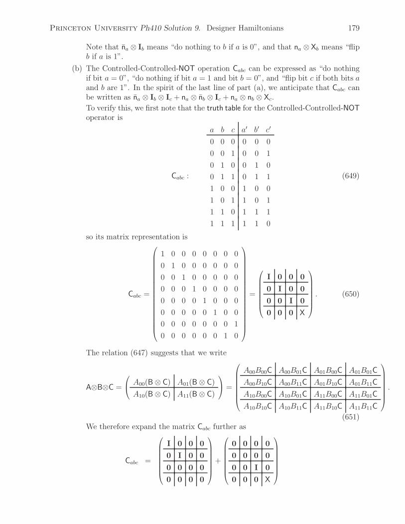
Princeton University Ph410 Solution 9. Designer Hamiltonians 179
Note that na ⊗ Ib means “do nothing to b if a is 0”, and that na ⊗ Xb means “flipb if a is 1”.
(b) The Controlled-Controlled-NOT operation Cabc can be expressed as “do nothingif bit a = 0”, “do nothing if bit a = 1 and bit b = 0”, and “flip bit c if both bits aand b are 1”. In the spirit of the last line of part (a), we anticipate that Cabc canbe written as na ⊗ Ib ⊗ Ic + na ⊗ nb ⊗ Ic + na ⊗ nb ⊗ Xc.
To verify this, we first note that the truth table for the Controlled-Controlled-NOToperator is
Cabc :
a b c a′ b′ c′
0 0 0 0 0 0
0 0 1 0 0 1
0 1 0 0 1 0
0 1 1 0 1 1
1 0 0 1 0 0
1 0 1 1 0 1
1 1 0 1 1 1
1 1 1 1 1 0
(649)
so its matrix representation is
Cabc =
⎛⎜⎜⎜⎜⎜⎜⎜⎜⎜⎜⎜⎜⎜⎜⎜⎜⎜⎜⎝
1 0 0 0 0 0 0 0
0 1 0 0 0 0 0 0
0 0 1 0 0 0 0 0
0 0 0 1 0 0 0 0
0 0 0 0 1 0 0 0
0 0 0 0 0 1 0 0
0 0 0 0 0 0 0 1
0 0 0 0 0 0 1 0
⎞⎟⎟⎟⎟⎟⎟⎟⎟⎟⎟⎟⎟⎟⎟⎟⎟⎟⎟⎠
=
⎛⎜⎜⎜⎜⎜⎜⎝
I 0 0 0
0 I 0 0
0 0 I 0
0 0 0 X
⎞⎟⎟⎟⎟⎟⎟⎠. (650)
The relation (647) suggests that we write
A⊗B⊗C =
⎛⎝ A00(B ⊗ C) A01(B ⊗ C)
A10(B ⊗ C) A11(B ⊗ C)
⎞⎠ =
⎛⎜⎜⎜⎜⎜⎜⎝
A00B00C A00B01C A01B00C A01B01C
A00B10C A00B11C A01B10C A01B11C
A10B00C A10B01C A11B00C A11B01C
A10B10C A10B11C A11B10C A11B11C
⎞⎟⎟⎟⎟⎟⎟⎠.
(651)We therefore expand the matrix Cabc further as
Cabc =
⎛⎜⎜⎜⎜⎜⎜⎝
I 0 0 0
0 I 0 0
0 0 0 0
0 0 0 0
⎞⎟⎟⎟⎟⎟⎟⎠
+
⎛⎜⎜⎜⎜⎜⎜⎝
0 0 0 0
0 0 0 0
0 0 I 0
0 0 0 X
⎞⎟⎟⎟⎟⎟⎟⎠
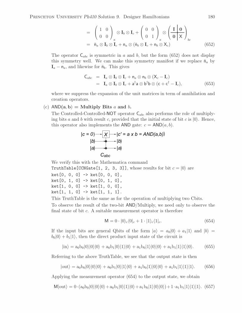
Princeton University Ph410 Solution 9. Designer Hamiltonians 180
=
⎛⎝ 1 0
0 0
⎞⎠a
⊗ Ib ⊗ Ic +
⎛⎝ 0 0
0 1
⎞⎠a
⊗⎛⎝ I 0
0 X
⎞⎠bc
= na ⊗ Ib ⊗ Ic + na ⊗ (nb ⊗ Ic + nb ⊗ Xc) (652)
The operator Cabc is symmetric in a and b, but the form (652) does not displaythis symmetry well. We can make this symmetry manifest if we replace na byIa − na, and likewise for nb. This gives
Cabc = Ia ⊗ Ib ⊗ Ic + na ⊗ nb ⊗ (Xc − Ic)
= Ia ⊗ Ib ⊗ Ic + a†a ⊗ b†b ⊗ (c + c† − Ic), (653)
where we suppress the expansion of the unit matrices in term of annihilation andcreation operators.
(c) AND(a,b) = Multiply Bits a and b.
The Controlled-Controlled-NOT operator Cabc also performs the role of multiply-ing bits a and b with result c, provided that the initial state of bit c is |0〉. Hence,this operator also implements the AND gate: c = AND(a, b).
We verify this with the Mathematica commandTruthTable[CCNGate[1, 2, 3, 3]], whose results for bit c = |0〉 are
ket[0, 0, 0] -> ket[0, 0, 0],
ket[0, 1, 0] -> ket[0, 1, 0],
ket[1, 0, 0] -> ket[1, 0, 0],
ket[1, 1, 0] -> ket[1, 1, 1].
This TruthTable is the same as for the operation of multiplying two Cbits.
To observe the result of the two-bit AND/Multiply, we need only to observe thefinal state of bit c. A suitable measurement operator is therefore
M = 0 · |0〉c〈0|c + 1 · |1〉c〈1|c. (654)
If the input bits are general Qbits of the form |a〉 = a0|0〉 + a1|1〉 and |b〉 =b0|0〉 + b1|1〉, then the direct product input state of the circuit is
|in〉 = a0b0|0〉|0〉|0〉 + a0b1|0〉|1〉|0〉 + a1b0|1〉|0〉|0〉 + a1b1|1〉|1〉|0〉. (655)
Referring to the above TruthTable, we see that the output state is then
|out〉 = a0b0|0〉|0〉|0〉 + a0b1|0〉|1〉|0〉 + a1b0|1〉|0〉|0〉 + a1b1|1〉|1〉|1〉. (656)
Applying the measurement operator (654) to the output state, we obtain
M|out〉 = 0 ·(a0b0|0〉|0〉|0〉+a0b1|0〉|1〉|0〉+a1b0|1〉|0〉|0〉)+1 ·a1b1|1〉|1〉|1〉. (657)
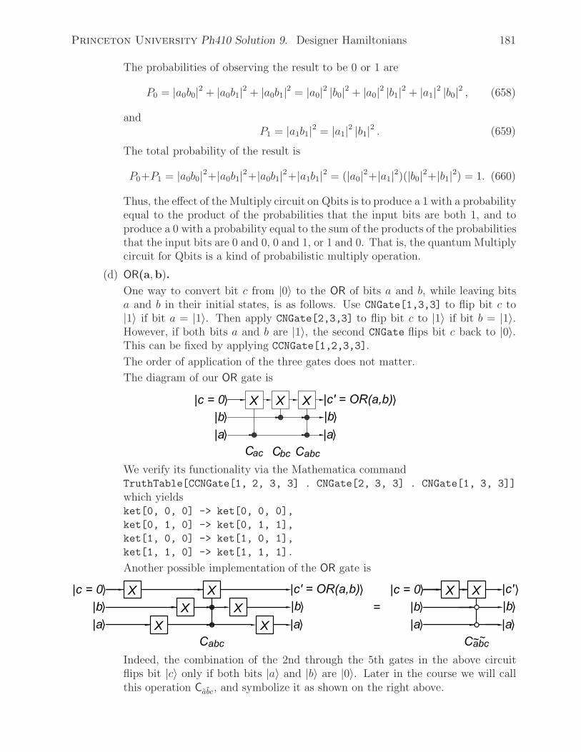
Princeton University Ph410 Solution 9. Designer Hamiltonians 181
The probabilities of observing the result to be 0 or 1 are
P0 = |a0b0|2 + |a0b1|2 + |a0b1|2 = |a0|2 |b0|2 + |a0|2 |b1|2 + |a1|2 |b0|2 , (658)
andP1 = |a1b1|2 = |a1|2 |b1|2 . (659)
The total probability of the result is
P0+P1 = |a0b0|2+|a0b1|2+|a0b1|2+|a1b1|2 = (|a0|2+|a1|2)(|b0|2+|b1|2) = 1. (660)
Thus, the effect of the Multiply circuit on Qbits is to produce a 1 with a probabilityequal to the product of the probabilities that the input bits are both 1, and toproduce a 0 with a probability equal to the sum of the products of the probabilitiesthat the input bits are 0 and 0, 0 and 1, or 1 and 0. That is, the quantum Multiplycircuit for Qbits is a kind of probabilistic multiply operation.
(d) OR(a,b).
One way to convert bit c from |0〉 to the OR of bits a and b, while leaving bitsa and b in their initial states, is as follows. Use CNGate[1,3,3] to flip bit c to|1〉 if bit a = |1〉. Then apply CNGate[2,3,3] to flip bit c to |1〉 if bit b = |1〉.However, if both bits a and b are |1〉, the second CNGate flips bit c back to |0〉.This can be fixed by applying CCNGate[1,2,3,3].
The order of application of the three gates does not matter.
The diagram of our OR gate is
We verify its functionality via the Mathematica commandTruthTable[CCNGate[1, 2, 3, 3] . CNGate[2, 3, 3] . CNGate[1, 3, 3]]
which yieldsket[0, 0, 0] -> ket[0, 0, 0],
ket[0, 1, 0] -> ket[0, 1, 1],
ket[1, 0, 0] -> ket[1, 0, 1],
ket[1, 1, 0] -> ket[1, 1, 1].
Another possible implementation of the OR gate is
Indeed, the combination of the 2nd through the 5th gates in the above circuitflips bit |c〉 only if both bits |a〉 and |b〉 are |0〉. Later in the course we will callthis operation Cabc, and symbolize it as shown on the right above.

Princeton University Ph410 Solution 9. Designer Hamiltonians 182
(e) Add Two 1-Bit Numbers.
The Controlled-NOT operator Cab also performs the role of addition modulo 2,with the result appearing as bit b′. This can be seen viaTruthTable[CNGate[1, 2, 2]]
which returnsket[0, 0] -> ket[0, 0],
ket[0, 1] -> ket[0, 1],
ket[1, 0] -> ket[1, 1],
ket[1, 1] -> ket[1, 0].
The remaining task is to “carry” the 1 that results from adding 1 to 1. For thiswe need an operator that produces a |1〉 only when both bits a and b are |1〉, andzero otherwise. Further, since we can’t copy the initial Qbits a and b, the desiredoperator should simply pass these bits on unaltered. On reflection, we see thatthe Controlled-Controlled-NOT operator is what we want.
A circuit for a quantum adder that adds bits a and b and presents the answer asc′b′ (i.e., the high-order bit is c′ = (a + b)1) is
Our adder gate is the product CijCijk, meaning that the Cijk is applied first. Toverify that we should use CNGate[1,2,3] . CCNGate[1,2,3,3] and notCCNGate[1,2,3,3] . CNGate[1,3,3], we executeTruthTable[CNGate[1, 2, 3] . CCNGate[1, 2, 3, 3]]
which returnsket[0, 0, 0] -> ket[0, 0, 0],
ket[0, 1, 0] -> ket[0, 1, 0],
ket[1, 0, 0] -> ket[1, 1, 0],
ket[1, 1, 0] -> ket[1, 0, 1].
The addends are the initial bits 1 and 3. The low-order bit of the answer isbit 2, and the high-order bit is bit 3. Thus, ket[1, 1, 0] -> ket[1, 0, 1]
corresponds to 1 + 1 = 10, as desired.
To observe the result of the two-bit ADD circuit, we need to observe the finalstate of bits b and c. A suitable measurement operator is therefore
A = 0 · |0〉b〈0|b · |0〉c〈0|c + 1 · |0〉b〈0|b · |1〉c〈1|c + 10 · |1〉b〈1|b · |0〉c〈0|c (661)
If the input bits are general Qbits of the form |a〉 = a0|0〉 + a1|1〉 and |b〉 =b0|0〉 + b1|1〉, then the input state of the circuit is
|in〉 = a0b0|0〉|0〉|0〉 + a0b1|0〉|1〉|0〉 + a1b0|1〉|0〉|0〉 + a1b1|1〉|1〉|0〉. (662)
Referring to the above TruthTable, we see that the output state is then
|out〉 = a0b0|0〉|0〉|0〉 + a0b1|0〉|0〉|1〉 + a1b0|1〉|0〉|1〉 + a1b1|1〉|1〉|0〉. (663)

Princeton University Ph410 Solution 9. Designer Hamiltonians 183
Applying the measurement operator (654) to the output state, we obtain
A|out〉 = 0 · a0b0|0〉|0〉|0〉 + 1 · (a0b1|0〉|0〉|1〉 + a1b0|1〉|0〉|1〉) + 10 · a1b1|1〉|1〉|0〉.(664)
The probabilities of observing the result to be 0, 1 or 10 are
P0 = |a0b0|2 , (665)
P1 = |a0b1|2 + |a1b0|2 , (666)
andP10 = |a1b1|2 . (667)
Thus, the effect of the Add circuit on Qbits is to produce a sum with a proba-bility equal to the probability of observing the corresponding addends. Like thequantum Multiply circuit, the quantum Add circuit for Qbits functions proba-bilistically.
A possible defect of the above circuit is that the initial value of the bit b isoverwritten. We could make a classical copy of the second addend bit using aControlled-NOT gate that acts on that bit and a fourth bit whose initial value is|0〉, as shown in the diagram below.
The action of this circuit on classical bits is the same as that of the previousadder. Thus,TruthTable[CNGate[1, 3, 4] . CCNGate[1, 3, 4, 4] . CNGate[2, 3, 4]]
returnsket[0, 0, 0, 0] -> ket[0, 0, 0, 0],
ket[0, 1, 0, 0] -> ket[0, 1, 1, 0],
ket[1, 0, 0, 0] -> ket[1, 0, 1, 0],
ket[1, 1, 0, 0] -> ket[1, 1, 0, 1].
To observe the result of the revised two-bit Add circuit, we need to observe thefinal state of bits c and d. A suitable measurement operator is therefore
A = 0 · |0〉c〈0|c · |0〉d〈0|d + 1 · |0〉c〈0|c · |1〉d〈1|d + 10 · |1〉c〈1|c · |0〉d〈0|d (668)
If the input bits are general Qbits of the form |a〉 = a0|0〉 + a1|1〉 and |b〉 =b0|0〉 + b1|1〉, then the direct product input state of the circuit is
|in〉 = a0b0|0〉|0〉|0〉|0〉+a0b1|0〉|1〉|0〉|0〉+a1b0|1〉|0〉|0〉|0〉+a1b1|1〉|1〉|0〉|0〉. (669)
Referring to the above TruthTable, we see that the output state is then
|out〉 = a0b0|0〉|0〉|0〉|0〉 + a0b1|0〉|1〉|0〉|1〉 + a1b0|1〉|0〉|0〉|1〉 + a1b1|1〉|1〉|1〉|0〉.(670)
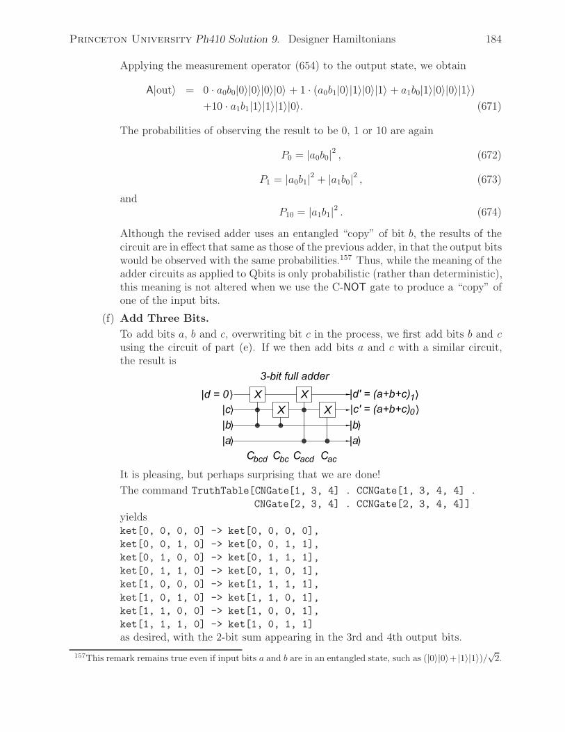
Princeton University Ph410 Solution 9. Designer Hamiltonians 184
Applying the measurement operator (654) to the output state, we obtain
A|out〉 = 0 · a0b0|0〉|0〉|0〉|0〉 + 1 · (a0b1|0〉|1〉|0〉|1〉 + a1b0|1〉|0〉|0〉|1〉)+10 · a1b1|1〉|1〉|1〉|0〉. (671)
The probabilities of observing the result to be 0, 1 or 10 are again
P0 = |a0b0|2 , (672)
P1 = |a0b1|2 + |a1b0|2 , (673)
andP10 = |a1b1|2 . (674)
Although the revised adder uses an entangled “copy” of bit b, the results of thecircuit are in effect that same as those of the previous adder, in that the output bitswould be observed with the same probabilities.157 Thus, while the meaning of theadder circuits as applied to Qbits is only probabilistic (rather than deterministic),this meaning is not altered when we use the C-NOT gate to produce a “copy” ofone of the input bits.
(f) Add Three Bits.
To add bits a, b and c, overwriting bit c in the process, we first add bits b and cusing the circuit of part (e). If we then add bits a and c with a similar circuit,the result is
It is pleasing, but perhaps surprising that we are done!
The command TruthTable[CNGate[1, 3, 4] . CCNGate[1, 3, 4, 4] .
CNGate[2, 3, 4] . CCNGate[2, 3, 4, 4]]
yieldsket[0, 0, 0, 0] -> ket[0, 0, 0, 0],
ket[0, 0, 1, 0] -> ket[0, 0, 1, 1],
ket[0, 1, 0, 0] -> ket[0, 1, 1, 1],
ket[0, 1, 1, 0] -> ket[0, 1, 0, 1],
ket[1, 0, 0, 0] -> ket[1, 1, 1, 1],
ket[1, 0, 1, 0] -> ket[1, 1, 0, 1],
ket[1, 1, 0, 0] -> ket[1, 0, 0, 1],
ket[1, 1, 1, 0] -> ket[1, 0, 1, 1]
as desired, with the 2-bit sum appearing in the 3rd and 4th output bits.
157This remark remains true even if input bits a and b are in an entangled state, such as (|0〉|0〉+ |1〉|1〉)/√2.
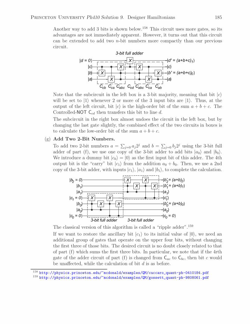
Princeton University Ph410 Solution 9. Designer Hamiltonians 185
Another way to add 3 bits is shown below.158 This circuit uses more gates, so itsadvantages are not immediately apparent. However, it turns out that this circuitcan be extended to add two n-bit numbers more compactly than our previouscircuit.
Note that the subcircuit in the left box is a 3-bit majority, meaning that bit |c〉will be set to |1〉 whenever 2 or more of the 3 input bits are |1〉. Thus, at theoutput of the left circuit, bit |c〉 is the high-order bit of the sum a + b + c. TheControlled-NOT Ccd then transfers this bit to line d.
The subcircuit in the right box almost undoes the circuit in the left box, but bychanging the last gate slightly, the combined effect of the two circuits in boxes isto calculate the low-order bit of the sum a + b+ c.
(g) Add Two 2-Bit Numbers.
To add two 2-bit numbers a =∑j=0 aj2
j and b =∑j=0 bj2
j using the 3-bit fulladder of part (f), we use one copy of the 3-bit adder to add bits |a0〉 and |b0〉.We introduce a dummy bit |c0〉 = |0〉 as the first input bit of this adder. The 4thoutput bit is the “carry” bit |c1〉 from the addition a0 + b0. Then, we use a 2ndcopy of the 3-bit adder, with inputs |c1〉, |a1〉 and |b1〉, to complete the calculation.
The classical version of this algorithm is called a “ripple adder”.159
If we want to restore the ancillary bit |c1〉 to its initial value of |0〉, we need anadditional group of gates that operate on the upper four bits, without changingthe first three of those bits. The desired circuit is no doubt closely related to thatof part (f) which sums the first three bits. In particular, we note that if the 4rthgate of the adder circuit of part (f) is changed from Cac to Cbc, then bit c wouldbe unaffected, while the calculation of bit d is as before.
158 http://physics.princeton.edu/~mcdonald/examples/QM/cuccaro_quant-ph-0410184.pdf159 http://physics.princeton.edu/~mcdonald/examples/QM/gossett_quant-ph-9808061.pdf
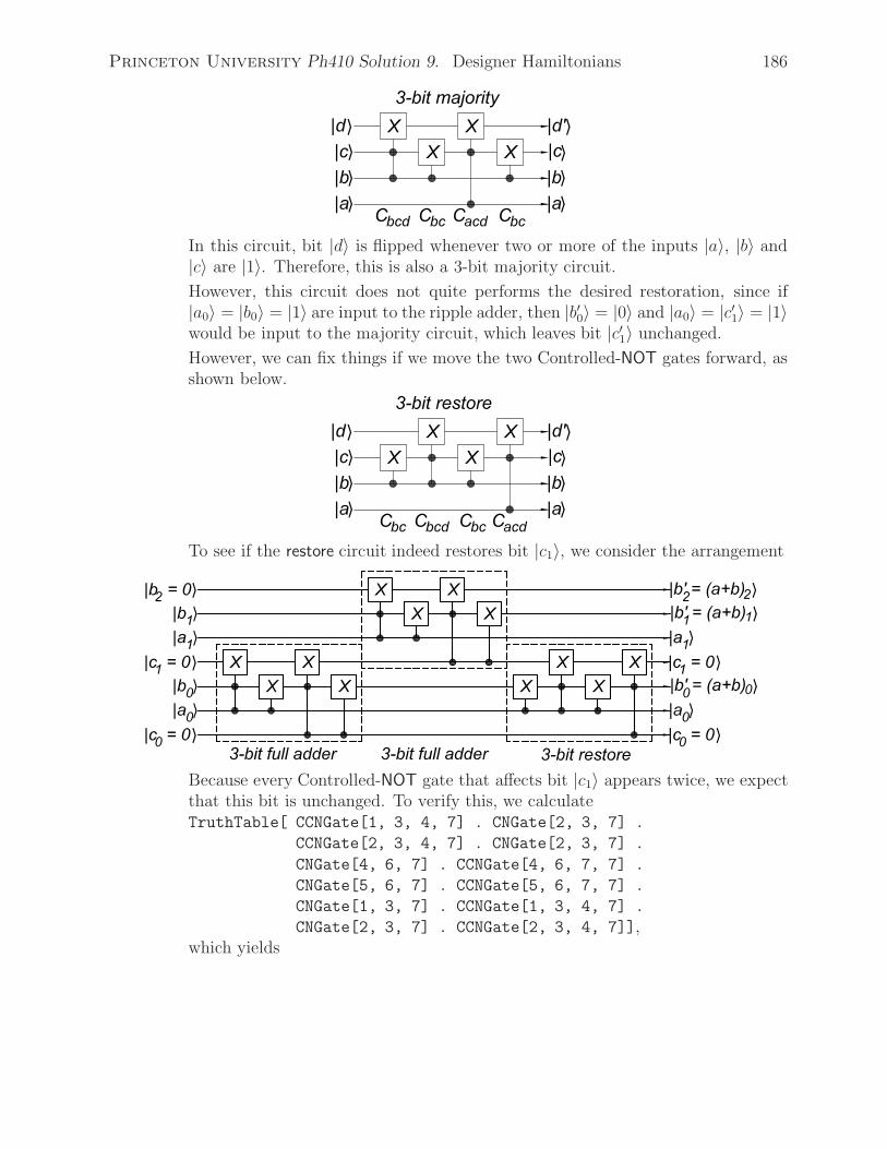
Princeton University Ph410 Solution 9. Designer Hamiltonians 186
In this circuit, bit |d〉 is flipped whenever two or more of the inputs |a〉, |b〉 and|c〉 are |1〉. Therefore, this is also a 3-bit majority circuit.
However, this circuit does not quite performs the desired restoration, since if|a0〉 = |b0〉 = |1〉 are input to the ripple adder, then |b′0〉 = |0〉 and |a0〉 = |c′1〉 = |1〉would be input to the majority circuit, which leaves bit |c′1〉 unchanged.
However, we can fix things if we move the two Controlled-NOT gates forward, asshown below.
To see if the restore circuit indeed restores bit |c1〉, we consider the arrangement
Because every Controlled-NOT gate that affects bit |c1〉 appears twice, we expectthat this bit is unchanged. To verify this, we calculateTruthTable[ CCNGate[1, 3, 4, 7] . CNGate[2, 3, 7] .
CCNGate[2, 3, 4, 7] . CNGate[2, 3, 7] .
CNGate[4, 6, 7] . CCNGate[4, 6, 7, 7] .
CNGate[5, 6, 7] . CCNGate[5, 6, 7, 7] .
CNGate[1, 3, 7] . CCNGate[1, 3, 4, 7] .
CNGate[2, 3, 7] . CCNGate[2, 3, 4, 7]],which yields

Princeton University Ph410 Solution 9. Designer Hamiltonians 187
ket[0, 0, 0, 0, 0, 0, 0] -> ket[0, 0, 0, 0, 0, 0, 0],
ket[0, 0, 1, 0, 0, 0, 0] -> ket[0, 0, 1, 0, 0, 0, 0],
ket[0, 1, 0, 0, 0, 0, 0] -> ket[0, 1, 1, 0, 0, 0, 0],
ket[0, 1, 1, 0, 0, 0, 0] -> ket[0, 1, 1, 0, 0, 1, 0],
ket[0, 0, 0, 0, 0, 1, 0] -> ket[0, 0, 0, 0, 0, 1, 0],
ket[0, 0, 1, 0, 0, 1, 0] -> ket[0, 0, 1, 0, 0, 1, 0],
ket[0, 1, 0, 0, 0, 1, 0] -> ket[0, 1, 1, 0, 0, 1, 0],
ket[0, 1, 1, 0, 0, 1, 0] -> ket[0, 1, 0, 0, 0, 0, 1],
ket[0, 0, 0, 0, 1, 0, 0] -> ket[0, 0, 0, 0, 1, 1, 0],
ket[0, 0, 1, 0, 1, 0, 0] -> ket[0, 0, 1, 0, 1, 1, 0],
ket[0, 1, 0, 0, 1, 0, 0] -> ket[0, 1, 1, 0, 1, 1, 0],
ket[0, 1, 1, 0, 1, 0, 0] -> ket[0, 1, 0, 0, 1, 0, 1],
ket[0, 0, 0, 0, 1, 1, 0] -> ket[0, 0, 0, 0, 1, 0, 1],
ket[0, 0, 1, 0, 1, 1, 0] -> ket[0, 0, 1, 0, 1, 0, 1],
ket[0, 1, 0, 0, 1, 1, 0] -> ket[0, 1, 1, 0, 1, 0, 1],
ket[0, 1, 1, 0, 1, 1, 0] -> ket[0, 1, 0, 0, 1, 1, 1].
The quantum computation literature160 shows a variant on the above circuit inwhich the 3-bit full adder of part (f) is split into a 3-bit carry and a 3-bit halfadder, that calculate the higher- and lower-order bits of the sum, respectively:
Note that a second 3-bit carry operation undoes the effect of the first. Hence, aripple adder could also be constructed with a cascade of 3-bit carry operations thatterminates in a 3-bit full adder for the highest-order bits, followed by an inversecascade of carry operations to reset the ancillary bits on all but the highest-orderbits of a and b to reset the ancillary bits. Also, 3-bit half adders must be insertedinto the inverse cascade so as to utilize the carry bits just before they are reset:
The two versions of the quantum ripple adders involve the same number of gates.
160 http://physics.princeton.edu/~mcdonald/examples/QM/vedral_pra_54_147_96.pdf
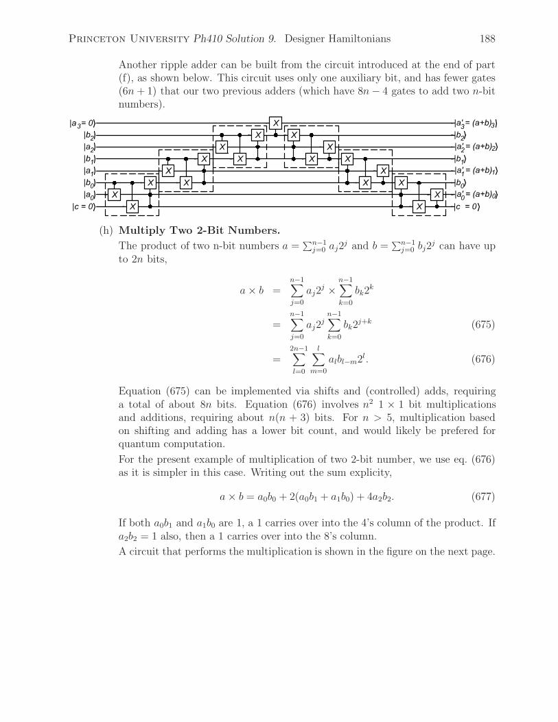
Princeton University Ph410 Solution 9. Designer Hamiltonians 188
Another ripple adder can be built from the circuit introduced at the end of part(f), as shown below. This circuit uses only one auxiliary bit, and has fewer gates(6n+ 1) that our two previous adders (which have 8n− 4 gates to add two n-bitnumbers).
(h) Multiply Two 2-Bit Numbers.
The product of two n-bit numbers a =∑n−1j=0 aj2
j and b =∑n−1j=0 bj2
j can have upto 2n bits,
a× b =n−1∑j=0
aj2j ×
n−1∑k=0
bk2k
=n−1∑j=0
aj2jn−1∑k=0
bk2j+k (675)
=2n−1∑l=0
l∑m=0
albl−m2l. (676)
Equation (675) can be implemented via shifts and (controlled) adds, requiringa total of about 8n bits. Equation (676) involves n2 1 × 1 bit multiplicationsand additions, requiring about n(n + 3) bits. For n > 5, multiplication basedon shifting and adding has a lower bit count, and would likely be prefered forquantum computation.
For the present example of multiplication of two 2-bit number, we use eq. (676)as it is simpler in this case. Writing out the sum explicity,
a× b = a0b0 + 2(a0b1 + a1b0) + 4a2b2. (677)
If both a0b1 and a1b0 are 1, a 1 carries over into the 4’s column of the product. Ifa2b2 = 1 also, then a 1 carries over into the 8’s column.
A circuit that performs the multiplication is shown in the figure on the next page.
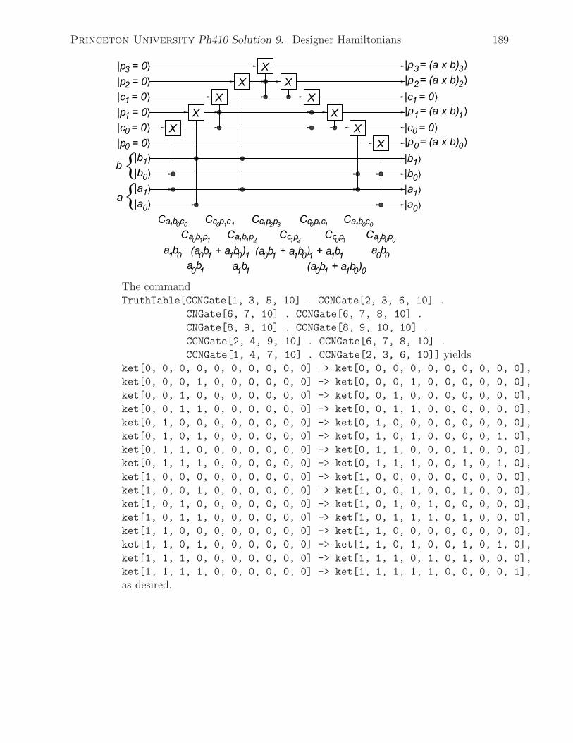
Princeton University Ph410 Solution 9. Designer Hamiltonians 189
The commandTruthTable[CCNGate[1, 3, 5, 10] . CCNGate[2, 3, 6, 10] .
CNGate[6, 7, 10] . CCNGate[6, 7, 8, 10] .
CNGate[8, 9, 10] . CCNGate[8, 9, 10, 10] .
CCNGate[2, 4, 9, 10] . CCNGate[6, 7, 8, 10] .
CCNGate[1, 4, 7, 10] . CCNGate[2, 3, 6, 10]] yieldsket[0, 0, 0, 0, 0, 0, 0, 0, 0, 0] -> ket[0, 0, 0, 0, 0, 0, 0, 0, 0, 0],
ket[0, 0, 0, 1, 0, 0, 0, 0, 0, 0] -> ket[0, 0, 0, 1, 0, 0, 0, 0, 0, 0],
ket[0, 0, 1, 0, 0, 0, 0, 0, 0, 0] -> ket[0, 0, 1, 0, 0, 0, 0, 0, 0, 0],
ket[0, 0, 1, 1, 0, 0, 0, 0, 0, 0] -> ket[0, 0, 1, 1, 0, 0, 0, 0, 0, 0],
ket[0, 1, 0, 0, 0, 0, 0, 0, 0, 0] -> ket[0, 1, 0, 0, 0, 0, 0, 0, 0, 0],
ket[0, 1, 0, 1, 0, 0, 0, 0, 0, 0] -> ket[0, 1, 0, 1, 0, 0, 0, 0, 1, 0],
ket[0, 1, 1, 0, 0, 0, 0, 0, 0, 0] -> ket[0, 1, 1, 0, 0, 0, 1, 0, 0, 0],
ket[0, 1, 1, 1, 0, 0, 0, 0, 0, 0] -> ket[0, 1, 1, 1, 0, 0, 1, 0, 1, 0],
ket[1, 0, 0, 0, 0, 0, 0, 0, 0, 0] -> ket[1, 0, 0, 0, 0, 0, 0, 0, 0, 0],
ket[1, 0, 0, 1, 0, 0, 0, 0, 0, 0] -> ket[1, 0, 0, 1, 0, 0, 1, 0, 0, 0],
ket[1, 0, 1, 0, 0, 0, 0, 0, 0, 0] -> ket[1, 0, 1, 0, 1, 0, 0, 0, 0, 0],
ket[1, 0, 1, 1, 0, 0, 0, 0, 0, 0] -> ket[1, 0, 1, 1, 1, 0, 1, 0, 0, 0],
ket[1, 1, 0, 0, 0, 0, 0, 0, 0, 0] -> ket[1, 1, 0, 0, 0, 0, 0, 0, 0, 0],
ket[1, 1, 0, 1, 0, 0, 0, 0, 0, 0] -> ket[1, 1, 0, 1, 0, 0, 1, 0, 1, 0],
ket[1, 1, 1, 0, 0, 0, 0, 0, 0, 0] -> ket[1, 1, 1, 0, 1, 0, 1, 0, 0, 0],
ket[1, 1, 1, 1, 0, 0, 0, 0, 0, 0] -> ket[1, 1, 1, 1, 1, 0, 0, 0, 0, 1],
as desired.
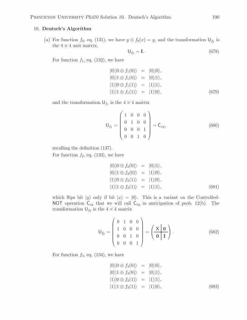
Princeton University Ph410 Solution 10. Deutsch’s Algorithm 190
10. Deutsch’s Algorithm
(a) For function f0, eq. (131), we have y ⊕ f0(x) = y, and the transformation Uf0 isthe 4 × 4 unit matrix,
Uf0 = I. (678)
For function f1, eq. (132), we have
|0〉|0 ⊕ f1(0)〉 = |0〉|0〉,|0〉|1 ⊕ f1(0)〉 = |0〉|1〉,|1〉|0 ⊕ f1(1)〉 = |1〉|1〉,|1〉|1 ⊕ f1(1)〉 = |1〉|0〉, (679)
and the transformation Uf1 is the 4 × 4 matrix
Uf1 =
⎛⎜⎜⎜⎜⎜⎜⎝
1 0 0 0
0 1 0 0
0 0 0 1
0 0 1 0
⎞⎟⎟⎟⎟⎟⎟⎠
= Cxy, (680)
recalling the definition (137).
For function f2, eq. (133), we have
|0〉|0 ⊕ f2(0)〉 = |0〉|1〉,|0〉|1 ⊕ f2(0)〉 = |1〉|0〉,|1〉|0 ⊕ f2(1)〉 = |1〉|0〉,|1〉|1 ⊕ f2(1)〉 = |1〉|1〉, (681)
which flips bit |y〉 only if bit |x〉 = |0〉. This is a variant on the Controlled-NOT operation Cxy that we will call Cxy in anticipation of prob. 12(b). Thetransformation Uf2 is the 4 × 4 matrix
Uf2 =
⎛⎜⎜⎜⎜⎜⎜⎝
0 1 0 0
1 0 0 0
0 0 1 0
0 0 0 1
⎞⎟⎟⎟⎟⎟⎟⎠
=
⎛⎝ X 0
0 I
⎞⎠ . (682)
For function f3, eq. (134), we have
|0〉|0 ⊕ f3(0)〉 = |0〉|0〉,|0〉|1 ⊕ f3(0)〉 = |0〉|1〉,|1〉|0 ⊕ f3(1)〉 = |1〉|1〉,|1〉|1 ⊕ f3(1)〉 = |1〉|0〉, (683)

Princeton University Ph410 Solution 10. Deutsch’s Algorithm 191
and the transformation Uf3 is the 4 × 4 matrix
Uf3 =
⎛⎜⎜⎜⎜⎜⎜⎝
0 1 0 0
1 0 0 0
0 0 0 1
0 0 1 0
⎞⎟⎟⎟⎟⎟⎟⎠
= Xy, (684)
recalling eq. (141).
(b) Only the transformation Uf2 = Cxy remains to be re-expressed in terms of theControlled-NOT operation Cxy. If we flip bit |x〉 prior to applying a Cxy operation,then bit |y〉 will be flipped when the initial |x〉 was |0〉 as desired. To restore state|x〉 to its initial value, we flip it a second time, but after the operation Cxy. Thus,
Cxy = XxCxyXx =
⎛⎝ 0 X
X 0
⎞⎠⎛⎝ I 0
0 X
⎞⎠⎛⎝ 0 X
X 0
⎞⎠
=
⎛⎝ 0 X
X 0
⎞⎠⎛⎝ 0 X
I 0
⎞⎠ =
⎛⎝ X 0
0 I
⎞⎠ = Uf2. (685)
(c) Diagrams for the four transformations Ufj found in part (b) are
(d) Note that the unitary transformation Uf is represented by real, symmetric ma-trices, and hence U−1 = U† = U. This suggests that a second application ofDeutsch’s transformation (135) may undo the effect of the first application. Butsince a measurement was made after the first application, we must look into thedetails.
Following the application of transformation (135) to the input bits |x〉 = |+〉 and|y〉 = |−〉, the measurement of the first bit yields (−1)f(0)|+〉 if f(0) = f(1) and(−1)f(0)|−〉 if f(0) = f(1). Hence, if f(0) = f(1), a second application of thetransformation (135), now using the measured bit as the input bit |x〉, will bringthat bit to [(−1)f(0)]2|+〉 = |+〉, which restores it to its initial value.
This suggests that we try the transformation (135) for the case where |x〉 =(−1)f(0)|−〉 and |y〉 = |−〉. Recalling eq. (142) we obtain
|x〉|y ⊕ f(x)〉 = (−1)f(0) (−1)f(0)|0〉 − (−1)f(1)|1〉√2
|0〉 − |1〉√2
. (686)

Princeton University Ph410 Solution 10. Deutsch’s Algorithm 192
Thus, if we apply the transformation (135) to the results of the measurement, weget the |x〉 = |+〉 and |y〉 = |−〉 when f(0) = f(1), and we get the result (686)when f(0) = f(1). In the latter case this also gives |x〉 = [(−1)f(0)]2|+〉 = |+〉and |y〉 = |−〉. Thus, simply applying transformation (135) to the results of themeasurement restores the input bits to their initial states.
If the effect of the measurement is that the phase factor (−1)f(0) is lost, thento restore the bits precisely a measurement of bit |x〉 should be made after thesecond application of transformation (135) to discard the phase factor introducedby that transformation.
(e) The output of Deutsch’s algorithm for input bits |x〉 = |+〉 and |y〉 = |−〉 is thestate (143), which has useful properties in the [|+〉, |−〉] basis. To bring this stateto the [|0〉, |1〉] basis we apply the Hadamard transformation,
H =1√2
⎛⎝ 1 1
1 −1
⎞⎠ , (687)
separately to each of the bits. Then,
(H|x〉)(H|y ⊕ f(x)〉) =(−1)f(0)|0〉 + (−1)f(1)|1〉√
2
|0〉 − |1〉√2
(688)
=
((−1)f(0) + (−1)f(1)
2|0〉 +
(−1)f(0) − (−1)f(1)
2|1〉)|1〉.
This has the desired result that a measurement of the first bit in the [|0〉, |1〉] basisyields |0〉 if f(0) = f(1) and |1〉 if f(0) = f(1).
If we wish to bring the second bit back to its initial state of |0〉, we could apply anadditional NOT transformation to this. A diagram for this algorithm is therefore,
Since this diagram is symmetric and reversible, it is clear that a second applicationof it would bring the final state of the first application back to the initial state.
(f) An “obvious” generalization of the circuit of part (e) to n input bits is the circuitshown below, which is called the Deutsch-Jozsa algorithm.

Princeton University Ph410 Solution 10. Deutsch’s Algorithm 193
The input state consists of the n-bit word |x〉n and the 1-bit state |y〉. The unitarytransformation Uf is
Uf |x〉n|y〉 = |x〉n|y ⊕ f(x)〉, (689)
where f(x) is a function that maps n bits onto 1 bit.
Based on our experience with Deutsch’s algorithm for the case that input state|x〉 has only 1 bit, we expect that by observing the n-bit output state of |x〉n wemay learn something useful about the n-to-1 function f .
We again prepare the state |y〉 that is input to Uf to be
|y〉 = HX|0〉 =|0〉 − |1〉√
2. (690)
Then, the output state of bit y, after applying the transformation Uf , is againgiven by eq. (142),
|y ⊕ f(x)〉 =|0 ⊕ f(x)〉 − |1 ⊕ f(x)〉√
2= (−1)f(x) |0〉 − |1〉√
2. (691)
The state |x〉n that is input to Uf is given by
|x〉n = H⊗n|0〉n =1
2n/2
2n−1∑j=0
|j〉n, (692)
recalling eq. (130). This is a linear combination of all possible n-bit basis states|j〉n. Hence, a single operation of Uf on this input state can tell us somethingabout f(x) for all possible values of x.
Using the states (692) and (690) as the input states, we have
Uf (H⊗n ⊗ HX)|0〉n|0〉 =
1
2n/2
2n−1∑j=0
(−1)f(j)|j〉n |0〉 − |1〉√2
. (693)
The hint is that this result may be particularly simple if function f is constant,i.e., if f(x) = f(0) for all values of x. In this case all n terms of the output stateare multiplied by the same phase factor (−1)f(0),
Uf (H⊗n ⊗HX)|0〉n|0〉 =
(−1)f(0)
2n/2
2n−1∑j=0
|j〉n |0〉 − |1〉√2
(f is constant). (694)
As shown in the figure on the previous page, we now apply a Hadamard transfor-mation to each of the final-state bits (plus a NOT transformation to the final bity). Since H2 = I, each of the n bits of the state |x〉 is restored to |0〉 (and the ybit is also restored to |0〉). That is,
(H⊗n ⊗ XH)Uf (H⊗n ⊗HX)|0〉n|0〉 = (−1)f(0)|0〉n|0〉 (f is constant). (695)
If we observe all n final-state bits of |x〉n in the circuit shown on the precedingpage, we will find them all to be |0〉 when function f is constant.

Princeton University Ph410 Solution 10. Deutsch’s Algorithm 194
Of course, we might also find that all n final-state bits of |x〉n are |0〉 for otherversions of the function f .
Our task now is to find a restriction on function f so that the circuit can neverproduce final states |x〉n with all bits |0〉. Then, a single application of the circuitcan distinguish between a constant function f and this restricted class of f .
When we apply the final Hadamard transformations to the general case (693) weobtain
(H⊗n ⊗ XH)Uf (H⊗n ⊗HX)|0〉n|0〉 =
1
2n/2
2n−1∑j=0
(−1)f(j)H⊗n|j〉n|0〉. (696)
Each n-bit basis state |j〉n can be written as a direct product,
|j〉n =n−1∏l=0
|jl〉, (16)
where jl is either 0 or 1. Then,
H⊗n|j〉n =n−1∏l=0
H|jl〉 =1
2n/2
n−1∏l=0
(|0〉 + (−1)jl|1〉) =1
2n/2
n−1∏l=0
1∑kl=0
(−1)jlkl|kl〉
=1
2n/2
2n−1∑k=0
(−1)∑
ljlkl|k〉n =
1
2n/2
2n−1∑k=0
(−1)j·k|k〉n
=1
2n/2
2n−1∑k=0
(−1)j�k|k〉n, (697)
noting that the scalar product j · k =∑l jlkl has the same effect as the product
j � k =∑l jlkl (mod 2) when used as the exponent of −1. Thus,
(H⊗n ⊗ XH)Uf (H⊗n ⊗HX)|0〉n|0〉 =
1
2n
2n−1∑j=0
(−1)f(j)2n−1∑k=0
(−1)j�k|k〉n|0〉. (698)
We desire that the result (698) does not contain a term with the state |k〉n = |0〉n.For this state the scalar product j � k vanishes for all j. Hence, if
2n−1∑j=0
(−1)f(j) = 0, (699)
i.e., if f(j) = 0 for exactly half of the basis states |j〉 (and f(j) = 1 for the otherhalf), then the function f is balanced and the result (698) does not contain thestate |0〉n.Hence, the Deutsch-Jozsa algorithm solves the problem of determining whetherthe n-to-1 function f is either balanced or constant in a single quantum evaluationof f (provided that we know in advance that f is one or the other of these types).
If we are to make this determination by classical evaluations of the function f , wemust make 2n−1 + 1 such evaluations. So it is often said that the Deutsch-Jozsa

Princeton University Ph410 Solution 10. Deutsch’s Algorithm 195
algorithm shows how a quantum computer could be 2n−1 + 1 times faster than aclassical computer.
Note however, that if we know that f is either balanced or constant, we knowthat it is balanced as soon as we find two different values of x that give differentvalues of f . If indeed f(x) is balanced and we make m evaluations of it withdifferent, random values of x, then the probability that all m evaluations yieldthe same value of f is 2/2m. If, say, we are satisfied to know whether f isbalanced or constant to 99.9% probability, this can be determined by only 10classical evaluations no matter how large the word size n is.

Princeton University Ph410 Solution 11. Universal Classical Gates 196
11. Universal Gates for Classical Computation
(a) The 2-Bit NAND Gate is Universal for Classical Computation.
One way to implement the NOT, AND and OR gates with NAND gates is
(b) The Controlled-Controlled-NOT Gate is Universal for Classical Com-putation.
A single Controlled-Controlled-NOT gate serves as a NAND gate if its third inputis initially |1〉.
If the third bit is initially |0〉, then we must be able to add a 1-bit NOT gatebefore the third input to the Controlled-Controlled-NOT gate.
We note that a Controlled-Controlled-NOT gate functions as a NOT gate for itsfirst input if its second and third inputs are |1〉, but not if they are |0〉.
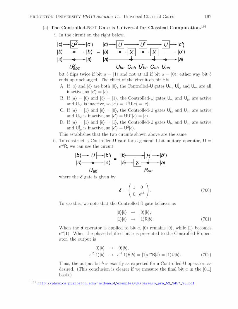
Princeton University Ph410 Solution 11. Universal Classical Gates 197
(c) The Controlled-NOT Gate is Universal for Classical Computation.161
i. In the circuit on the right below,
bit b flips twice if bit a = |1〉 and not at all if bit a = |0〉; either way bit bends up unchanged. The effect of the circuit on bit c is
A. If |a〉 and |b〉 are both |0〉, the Controlled-U gates Ubc, U†bc and Uac are all
inactive, so |c′〉 = |c〉.B. If |a〉 = |0〉 and |b〉 = |1〉, the Controlled-U gates Ubc and U†
bc are activeand Uac is inactive, so |c′〉 = U†U|c〉 = |c〉.
C. If |a〉 = |1〉 and |b〉 = |0〉, the Controlled-U gates U†bc and Uac are active
and Ubc is inactive, so |c′〉 = UU†|c〉 = |c〉.D. If |a〉 = |1〉 and |b〉 = |1〉, the Controlled-U gates Ubc and Uac are active
and U†bc is inactive, so |c′〉 = U2|c〉.
This establishes that the two circuits shown above are the same.
ii. To construct a Controlled-U gate for a general 1-bit unitary operator, U =eiδR, we can use the circuit
where the δ gate is given by
δ =
⎛⎝ 1 0
0 eiδ
⎞⎠ . (700)
To see this, we note that the Controlled-R gate behaves as
|0〉|b〉 → |0〉|b〉,|1〉|b〉 → |1〉R|b〉. (701)
When the δ operator is applied to bit a, |0〉 remains |0〉, while |1〉 becomeseiδ|1〉. When the phased-shifted bit a is presented to the Controlled-R oper-ator, the output is
|0〉|b〉 → |0〉|b〉,eiδ|1〉|b〉 → eiδ|1〉R|b〉 = |1〉eiδR|b〉 = |1〉U|b〉. (702)
Thus, the output bit b is exactly as expected for a Controlled-U operator, asdesired. (This conclusion is clearer if we measure the final bit a in the [0,1]basis.)
161 http://physics.princeton.edu/~mcdonald/examples/QM/barenco_pra_52_3457_95.pdf
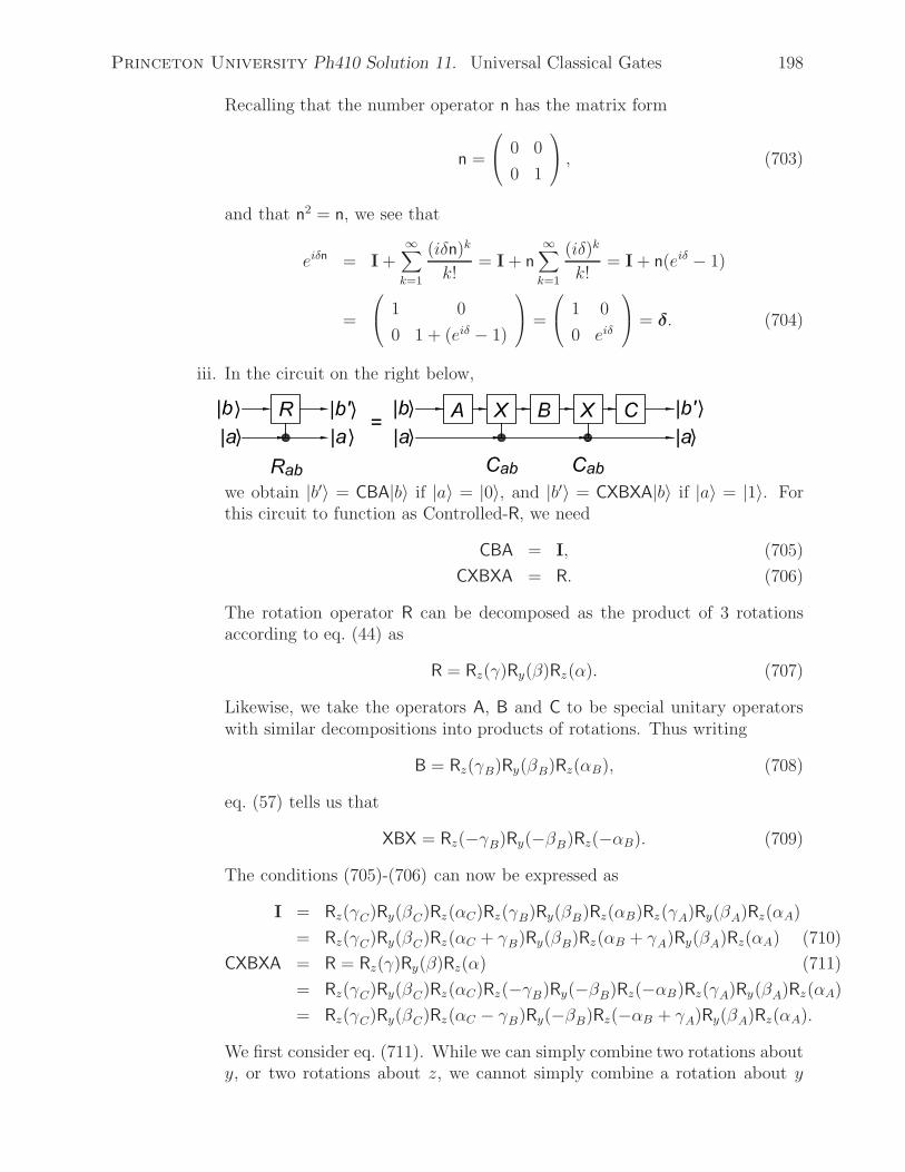
Princeton University Ph410 Solution 11. Universal Classical Gates 198
Recalling that the number operator n has the matrix form
n =
⎛⎝ 0 0
0 1
⎞⎠ , (703)
and that n2 = n, we see that
eiδn = I +∞∑k=1
(iδn)k
k!= I + n
∞∑k=1
(iδ)k
k!= I + n(eiδ − 1)
=
⎛⎝ 1 0
0 1 + (eiδ − 1)
⎞⎠ =
⎛⎝ 1 0
0 eiδ
⎞⎠ = δ. (704)
iii. In the circuit on the right below,
we obtain |b′〉 = CBA|b〉 if |a〉 = |0〉, and |b′〉 = CXBXA|b〉 if |a〉 = |1〉. Forthis circuit to function as Controlled-R, we need
CBA = I, (705)
CXBXA = R. (706)
The rotation operator R can be decomposed as the product of 3 rotationsaccording to eq. (44) as
R = Rz(γ)Ry(β)Rz(α). (707)
Likewise, we take the operators A, B and C to be special unitary operatorswith similar decompositions into products of rotations. Thus writing
B = Rz(γB)Ry(βB)Rz(αB), (708)
eq. (57) tells us that
XBX = Rz(−γB)Ry(−βB)Rz(−αB). (709)
The conditions (705)-(706) can now be expressed as
I = Rz(γC)Ry(βC)Rz(αC)Rz(γB)Ry(βB)Rz(αB)Rz(γA)Ry(βA)Rz(αA)
= Rz(γC)Ry(βC)Rz(αC + γB)Ry(βB)Rz(αB + γA)Ry(βA)Rz(αA) (710)
CXBXA = R = Rz(γ)Ry(β)Rz(α) (711)
= Rz(γC)Ry(βC)Rz(αC)Rz(−γB)Ry(−βB)Rz(−αB)Rz(γA)Ry(βA)Rz(αA)
= Rz(γC)Ry(βC)Rz(αC − γB)Ry(−βB)Rz(−αB + γA)Ry(βA)Rz(αA).
We first consider eq. (711). While we can simply combine two rotations abouty, or two rotations about z, we cannot simply combine a rotation about y

Princeton University Ph410 Solution 11. Universal Classical Gates 199
with a rotation about z. Thus, to collapse the last line of eq. (711) onto thefirst, we will have to take some rotations to be trivial. For example, we set
βA = 0, and αC − γB = 0. (712)
Then, eq. (711) reduces to
Rz(γ)Ry(β)Rz(α) = Rz(γC)Ry(βC − βB)Rz(−αB + γA + αA). (713)
This equation is satisfied provided that
γC = γ, βC − βB = β, and − αB + γA + αA = α. (714)
Our knowledge thus far can be summarized as
αC = γB , αB = αA + γA − α, αA = ?
βC = βB + β, βB = ? βA = 0,
γC = γ, γB = ? γA = ?
(715)
With this, eq. (710) becomes
I = Rz(γ)Ry(βB + β)Rz(2γB)Ry(βB)Rz(αA + γA − α)Rz(γA)Rz(αA)
= Rz(γ)Ry(βB + β)Rz(2γB)Ry(βB)Rz(2αA + 2γA − α). (716)
To collapse this further, we set
γB = 0 = αC . (717)
Equation (716) is now
I = Rz(γ)Ry(2βB + β)Rz(2αA + 2γA − α). (718)
To collapse this to the identity, we set
βB = −β2, αA + γA =
α− γ
2. (719)
The second equation of this can be satisfied by taking
αA =α
2, γA = −γ
2. (720)
The solution is
αC = 0, αB = −α+γ2, αA = α
2,
βC = β2, βB = −β
2, βA = 0,
γC = γ, γB = 0, γA = −γ2,
(721)

Princeton University Ph410 Solution 11. Universal Classical Gates 200
A = Rz
(α− γ
2
), (722)
B = Ry
(−β
2
)Rz
(−α+ γ
2
), (723)
C = Rz(γ)Ry
(β
2
). (724)
As a check,
CBA = Rz(γ)Ry
(β
2
)· Ry
(−β
2
)Rz
(−α+ γ
2
)· Rz
(α − γ
2
)
= Rz(γ)Rz(−γ) = I, (725)
CXBXA = Rz(γ)Ry
(β
2
)· Ry
(β
2
)Rz
(α+ γ
2
)· Rz
(α− γ
2
)
= Rz(γ)Ry(β)Rz(α) = R. (726)
This establishes that the two circuits in the figure 2 pages ago are identical.
iv. Using eq. (449), the NOT operator can be written.
X = σx = −iRx(π) = e−iπ/2Rx(π). (727)
Taking the square root, we obtain
√X = e−iπ/4Rx(π/2) =
1 − i√2
⎛⎝ 1√
2i√2
i√2
1√2
⎞⎠ =
1
2
⎛⎝ 1 − i 1 + i
1 + i 1 − i
⎞⎠
= e−iπ/4Rz(π/2)Ry(π/2)Rz(−π/2), (728)
recalling eq. (453). To represent√
X in the general form e−iδRz(γ)Ry(β)Rz(α)we use
α = −π2, β =
π
2, γ =
π
2, δ = −π
4. (729)
The 1-bit operators needed for the construction of the Controlled-√
X operatoras in sec. ii-iii are
A = Rz
(α− γ
2
)= Rz(−π), (730)
B = Ry
(−β
2
)Rz
(−α+ γ
2
)= Ry
(−π
4
), (731)
C = Rz(γ)Ry
(β
2
)= Rz(π)Ry
(π
4
), (732)
δ =
⎛⎝ 1 0
0 eiδ
⎞⎠ =
⎛⎝ 1 0
0 e−iπ/4
⎞⎠ . (733)

Princeton University Ph410 Solution 12. Universal Quantum Gates 201
12. Universal Gates for Quantum Computation
(a) All 1-Bit Quantum Gates Can Be Built from the H and σ1/4z Gates.162
σ−1/4z σ1/4
x = σ−1/4z Hσ1/4
z H
=1
2
⎛⎝ 1 0
0 e−iπ/4
⎞⎠⎛⎝ 1 1
1 −1
⎞⎠⎛⎝ 1 0
0 eiπ/4
⎞⎠⎛⎝ 1 1
1 −1
⎞⎠
=1
2
⎛⎝ 1 0
0 e−iπ/4
⎞⎠⎛⎝ 1 1
1 −1
⎞⎠⎛⎝ 1 1
eiπ/4 −eiπ/4
⎞⎠
=1
2
⎛⎝ 1 0
0 e−iπ/4
⎞⎠⎛⎝ 1 + eiπ/4 1 − eiπ/4
1 − eiπ/4 1 + eiπ/4
⎞⎠
=1
2
⎛⎝ 1 + eiπ/4 1 − eiπ/4
e−iπ/4 − 1 e−iπ/4 + 1
⎞⎠ =
⎛⎝ eiπ/8 cos π
8−ieiπ/8 sin π
8
−ie−iπ/8 sin π8
e−iπ/8 cos π8
⎞⎠
=
⎛⎝ cos2 π
8+ i sin π
8cos π
8−i sin π
8(cos π
8+ i sin π
8)
−i sin π8(cos π
8− i sin π
8) cos2 π
8− i sin π
8cos π
8
⎞⎠ . (734)
We desire this to be of the form
eiθ2u·σ = cos
θ
2I + i sin
θ
2(uxσx + uyσy + uzσz). (735)
Clearly we set
cosθ
2= cos2 π
8=
1 + cos π4
2=
2 +√
2
4. (736)
Corresponding to this, we have
sinθ
2=
√1 − cos2
θ
2=
√1 − cos4
π
8= sin
π
8
√1 + cos2
π
8. (737)
Using eqs. (736)-(737) in eq. (734), we can write
σ−1/4z σ1/4
x =
⎛⎜⎝ cos θ
2+ i sin θ
2
cos π8√
1+cos2 π8
i sin θ2
− cos π8−i sin π
8√1+cos2 π
8
i sin θ2
− cos π8+i sin π
8√1+cos2 π
8
cos θ2
+ i sin θ2
− cos π8√
1+cos2 π8
⎞⎟⎠
= cosθ
2I + i sin
θ
2
⎛⎝− cos π
8σx + sin π
8σy + cos π
8σz√
1 + cos2 π8
⎞⎠ . (738)
Comparing with eq. (735), we see that the axis of rotation has unit vector
u =(− cos π
8, sin π
8, cos π
8)√
1 + cos2 π8
, (739)
162 http://physics.princeton.edu/~mcdonald/examples/QM/boykin_quant-ph-9906054.pdf
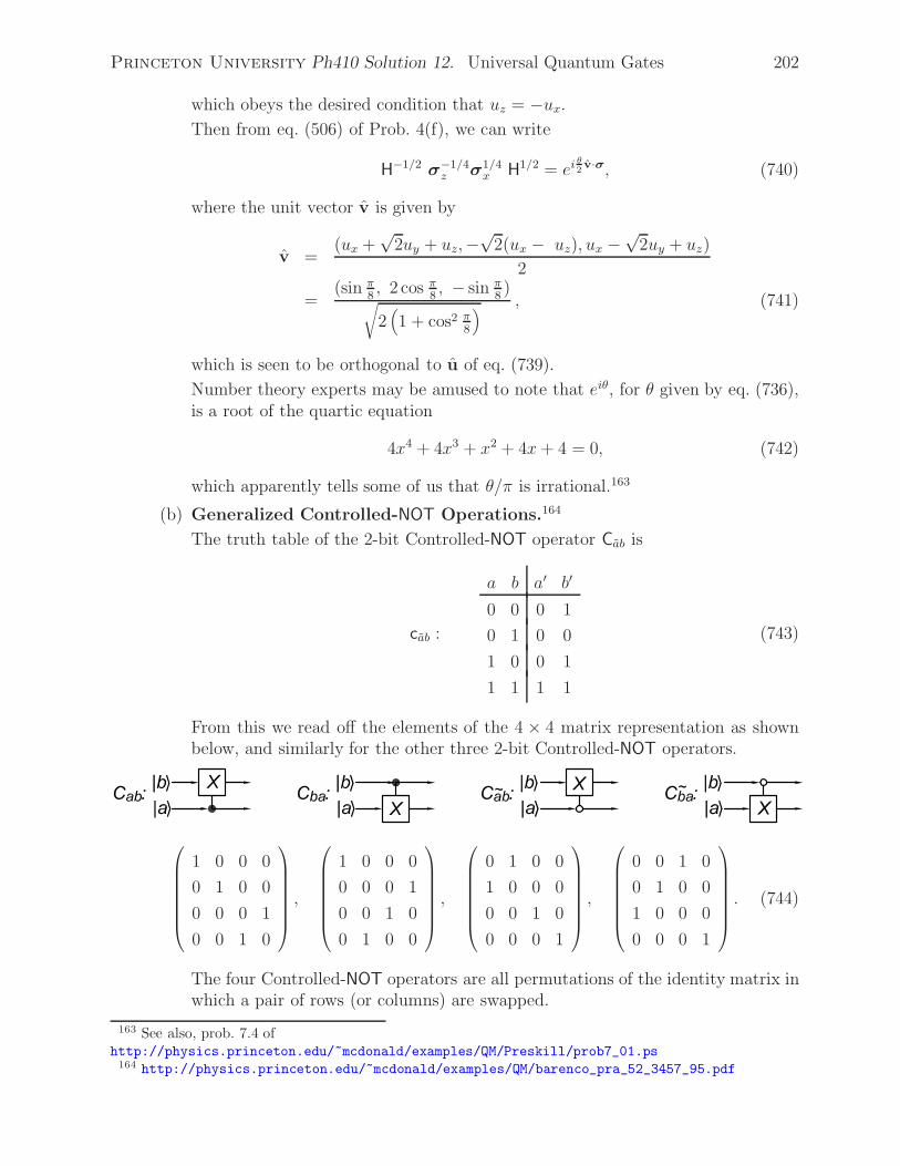
Princeton University Ph410 Solution 12. Universal Quantum Gates 202
which obeys the desired condition that uz = −ux.Then from eq. (506) of Prob. 4(f), we can write
H−1/2 σ−1/4z σ1/4
x H1/2 = eiθ2v·σ, (740)
where the unit vector v is given by
v =(ux +
√2uy + uz,−
√2(ux − uz), ux −
√2uy + uz)
2
=(sin π
8, 2 cos π
8, − sin π
8)√
2(1 + cos2 π
8
) , (741)
which is seen to be orthogonal to u of eq. (739).
Number theory experts may be amused to note that eiθ, for θ given by eq. (736),is a root of the quartic equation
4x4 + 4x3 + x2 + 4x+ 4 = 0, (742)
which apparently tells some of us that θ/π is irrational.163
(b) Generalized Controlled-NOT Operations.164
The truth table of the 2-bit Controlled-NOT operator Cab is
cab :
a b a′ b′
0 0 0 1
0 1 0 0
1 0 0 1
1 1 1 1
(743)
From this we read off the elements of the 4 × 4 matrix representation as shownbelow, and similarly for the other three 2-bit Controlled-NOT operators.
⎛⎜⎜⎜⎜⎜⎜⎝
1 0 0 0
0 1 0 0
0 0 0 1
0 0 1 0
⎞⎟⎟⎟⎟⎟⎟⎠,
⎛⎜⎜⎜⎜⎜⎜⎝
1 0 0 0
0 0 0 1
0 0 1 0
0 1 0 0
⎞⎟⎟⎟⎟⎟⎟⎠,
⎛⎜⎜⎜⎜⎜⎜⎝
0 1 0 0
1 0 0 0
0 0 1 0
0 0 0 1
⎞⎟⎟⎟⎟⎟⎟⎠,
⎛⎜⎜⎜⎜⎜⎜⎝
0 0 1 0
0 1 0 0
1 0 0 0
0 0 0 1
⎞⎟⎟⎟⎟⎟⎟⎠. (744)
The four Controlled-NOT operators are all permutations of the identity matrix inwhich a pair of rows (or columns) are swapped.
163 See also, prob. 7.4 ofhttp://physics.princeton.edu/~mcdonald/examples/QM/Preskill/prob7_01.ps
164 http://physics.princeton.edu/~mcdonald/examples/QM/barenco_pra_52_3457_95.pdf
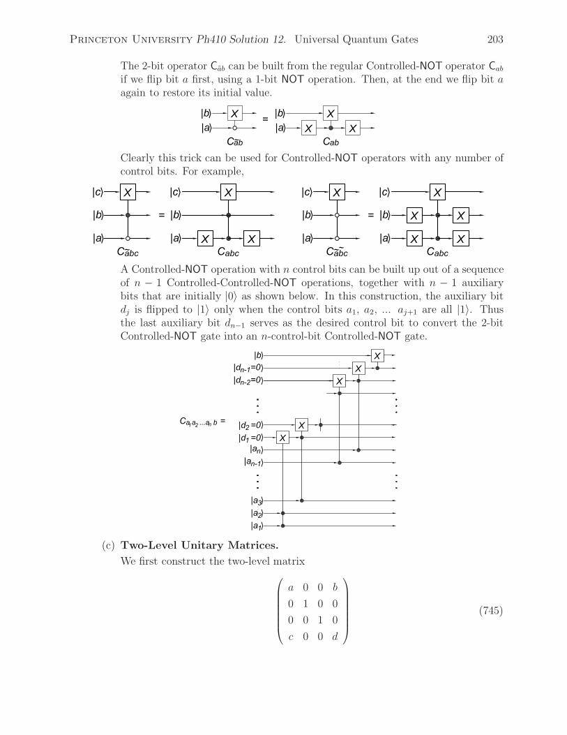
Princeton University Ph410 Solution 12. Universal Quantum Gates 203
The 2-bit operator Cab can be built from the regular Controlled-NOT operator Cabif we flip bit a first, using a 1-bit NOT operation. Then, at the end we flip bit aagain to restore its initial value.
Clearly this trick can be used for Controlled-NOT operators with any number ofcontrol bits. For example,
A Controlled-NOT operation with n control bits can be built up out of a sequenceof n − 1 Controlled-Controlled-NOT operations, together with n − 1 auxiliarybits that are initially |0〉 as shown below. In this construction, the auxiliary bitdj is flipped to |1〉 only when the control bits a1, a2, ... aj+1 are all |1〉. Thusthe last auxiliary bit dn−1 serves as the desired control bit to convert the 2-bitControlled-NOT gate into an n-control-bit Controlled-NOT gate.
(c) Two-Level Unitary Matrices.
We first construct the two-level matrix⎛⎜⎜⎜⎜⎜⎜⎝
a 0 0 b
0 1 0 0
0 0 1 0
c 0 0 d
⎞⎟⎟⎟⎟⎟⎟⎠
(745)
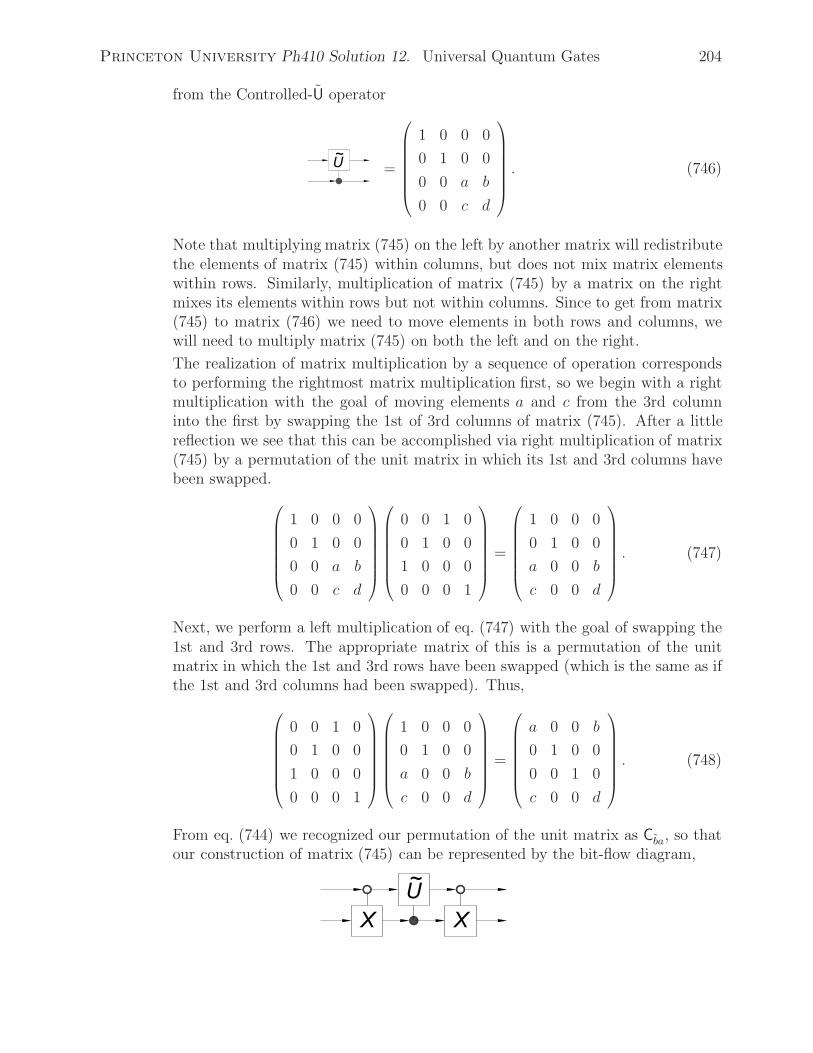
Princeton University Ph410 Solution 12. Universal Quantum Gates 204
from the Controlled-U operator
=
⎛⎜⎜⎜⎜⎜⎜⎝
1 0 0 0
0 1 0 0
0 0 a b
0 0 c d
⎞⎟⎟⎟⎟⎟⎟⎠. (746)
Note that multiplying matrix (745) on the left by another matrix will redistributethe elements of matrix (745) within columns, but does not mix matrix elementswithin rows. Similarly, multiplication of matrix (745) by a matrix on the rightmixes its elements within rows but not within columns. Since to get from matrix(745) to matrix (746) we need to move elements in both rows and columns, wewill need to multiply matrix (745) on both the left and on the right.
The realization of matrix multiplication by a sequence of operation correspondsto performing the rightmost matrix multiplication first, so we begin with a rightmultiplication with the goal of moving elements a and c from the 3rd columninto the first by swapping the 1st of 3rd columns of matrix (745). After a littlereflection we see that this can be accomplished via right multiplication of matrix(745) by a permutation of the unit matrix in which its 1st and 3rd columns havebeen swapped.
⎛⎜⎜⎜⎜⎜⎜⎝
1 0 0 0
0 1 0 0
0 0 a b
0 0 c d
⎞⎟⎟⎟⎟⎟⎟⎠
⎛⎜⎜⎜⎜⎜⎜⎝
0 0 1 0
0 1 0 0
1 0 0 0
0 0 0 1
⎞⎟⎟⎟⎟⎟⎟⎠
=
⎛⎜⎜⎜⎜⎜⎜⎝
1 0 0 0
0 1 0 0
a 0 0 b
c 0 0 d
⎞⎟⎟⎟⎟⎟⎟⎠. (747)
Next, we perform a left multiplication of eq. (747) with the goal of swapping the1st and 3rd rows. The appropriate matrix of this is a permutation of the unitmatrix in which the 1st and 3rd rows have been swapped (which is the same as ifthe 1st and 3rd columns had been swapped). Thus,
⎛⎜⎜⎜⎜⎜⎜⎝
0 0 1 0
0 1 0 0
1 0 0 0
0 0 0 1
⎞⎟⎟⎟⎟⎟⎟⎠
⎛⎜⎜⎜⎜⎜⎜⎝
1 0 0 0
0 1 0 0
a 0 0 b
c 0 0 d
⎞⎟⎟⎟⎟⎟⎟⎠
=
⎛⎜⎜⎜⎜⎜⎜⎝
a 0 0 b
0 1 0 0
0 0 1 0
c 0 0 d
⎞⎟⎟⎟⎟⎟⎟⎠. (748)
From eq. (744) we recognized our permutation of the unit matrix as Cba, so thatour construction of matrix (745) can be represented by the bit-flow diagram,

Princeton University Ph410 Solution 12. Universal Quantum Gates 205
Similarly, to construct the two-level matrix
⎛⎜⎜⎜⎜⎜⎜⎝
1 0 0 0
0 a b 0
0 c d 0
0 0 0 1
⎞⎟⎟⎟⎟⎟⎟⎠
(749)
from the Controlled-U operator
=
⎛⎜⎜⎜⎜⎜⎜⎝
1 0 0 0
0 a 0 b
0 0 1 0
0 c 0 d
⎞⎟⎟⎟⎟⎟⎟⎠, (750)
we need to multiply matrix (749) on the left and right by the permutation of theunit matrix in which the 3rd and 4th columns (or rows) are swapped,
⎛⎜⎜⎜⎜⎜⎜⎝
1 0 0 0
0 1 0 0
0 0 0 1
0 0 1 0
⎞⎟⎟⎟⎟⎟⎟⎠, (751)
which is, of course, just the basic Controlled-NOT operator Cab. Thus, the bit-flowdiagram to produce matrix (749) is
When U = X, we see that U of eq. (749) is the SWAP operation Sab introducedin prob. 9(c) and written as a 4 × 4 matrix in eq. (572). The bit-flow diagramfollowing eq. (576) is a special case of the diagram immediately above.
With the spirit of the above constructions in mind, we readily see that the two-level matrix (745) can be built using any of the four Controlled-U operators to-gether with appropriate Controlled-NOT operators,
and likewise the two-level matrix (749) can be built four ways,
We end this part with a brief summary of the procedure to build up any 2n × 2n
two-level matrix U from the 1-bit unitary matrix U.

Princeton University Ph410 Solution 12. Universal Quantum Gates 206
First, we note that a generalized Controlled-NOT operator is a two-level operatorthat flips a single bit of an n-bit state if the other bits match the control-bitpattern. These operators are permutations of the identity matrix in which onepair of rows (or columns), say rows j and k, have been swapped. The effect ofapplying this Controlled-NOT operator on the left of an arbitrary matrix U is toswap its rows j and k. Or, if the Controlled-NOT operator is applied on the rightof U, its columns j and k will be swapped. Then, applying the Controlled-NOToperator to both the left and right of U will swap both its rows and columns jand k.
Similarly, a generalized Controlled-U operator is a two-level operator that appliesan arbitrary 1-bit operator U to a specified bit of an n-bit state if the other bitsmatch the control-bit pattern.
Turning to a general 2n × 2n two-level matrix U such as shown in eq. (752), weconsider the nontrivial row indices j and k as binary numbers. If these numbersare the same except for one bit being a 0 in one case and a 1 in the other, thenU is the same as a Controlled-U operator where the control bits are equal to thecommon bits in the binary representation of j and k.
Utwo−level =
⎛⎜⎜⎜⎜⎜⎜⎜⎜⎜⎜⎜⎜⎜⎜⎜⎜⎜⎜⎜⎜⎜⎝
1 ... 0 ... 0 ... 0 ... 0
... ... ... ... ... ... ... ... ...
0 ... a ... 0 ... b ... 0
... ... ... ... ... ... ... ... ...
0 ... 0 ... 1 ... 0 ... 0
... ... ... ... ... ... ... ... ...
0 ... c ... 0 ... d ... 0
... ... ... ... ... ... ... ... ...
0 ... 0 ... 0 ... 0 ... 1
⎞⎟⎟⎟⎟⎟⎟⎟⎟⎟⎟⎟⎟⎟⎟⎟⎟⎟⎟⎟⎟⎟⎠
, U =
⎛⎝ a b
c d
⎞⎠ . (752)
If the binary representations of j and k differ in more than one bit, then we needto perform a sequence of bit flips on, say, index j, using appropriate generalizedControlled-NOT operators until the flipped j differs from k in only one digit. Wecan then construct U using the Controlled-U operator associated with the flippedj, together with the sequence of generalized Controlled-NOT operators needed toproduce the flipped j. This sequence of operators must be applied symmetricallyto both the left and right of the Controlled-U operator so as to move both therows and columns from their location in the Controlled-U operator to their desiredlocation in U.
When I wrote the above, I believed that I understood it. But can anyone elsefollow it?

Princeton University Ph410 Solution 13. The Bernstein-Vazirani Problem 207
13. The Bernstein-Vazirani Problem
(a) To implement fa(x) = a · x (mod 2) we recall that a Controlled-Controlled-NOToperation flips the target bit if the product of the control bits is 1. Also, additionmodulo 2 on a set of bits can be performed by flipping the sum bit once for each 1bit in the set. Hence, a sequence of Controlled-Controlled-NOT operations whosecontrol bits are corresponding bits of |a〉 and |x〉, and whose target bit is |y〉,performs the function fa(x).
If we regard a as fixed, the above circuit could be simplified by replacing theControlled-Controlled-NOT gates by Controlled-NOT gates, which are only neededfor a bit |xj〉 if aj = 1.
If the initial state of bit |y〉 had been |1〉, the final state of bit |y〉 would be flippedcompared to the case that |y〉 = |0〉 initially. That is, in general, |y〉 → |y⊕fa(x)〉.Summarizing the entire process as a unitary operator Ufa , we have
Ufa |a〉|x〉|y〉 = |a〉|x〉|y ⊕ fa(x)〉. (166)
(b) To demonstrate the identity
we note that applying the Hadamard operation,
H =1√2
⎛⎝ 1 1
1 −1
⎞⎠ , (753)

Princeton University Ph410 Solution 13. The Bernstein-Vazirani Problem 208
to both input lines is described by the 4 × 4 matrix (recall eq. (647))
H⊗2 = H ⊗ H =1
2
⎛⎜⎜⎜⎜⎜⎜⎜⎝
1 1 1 1
1 −1 1 −1
1 1 −1 −1
1 −1 −1 1
⎞⎟⎟⎟⎟⎟⎟⎟⎠. (754)
Then, recalling eqs. (552) and (574), we have
H⊗2CabH⊗2 =
1
4
⎛⎜⎜⎜⎜⎜⎜⎝
1 1 1 1
1 −1 1 −1
1 1 −1 −1
1 −1 −1 1
⎞⎟⎟⎟⎟⎟⎟⎠
⎛⎜⎜⎜⎜⎜⎜⎝
1 0 0 0
0 1 0 0
0 0 0 1
0 0 1 0
⎞⎟⎟⎟⎟⎟⎟⎠
⎛⎜⎜⎜⎜⎜⎜⎝
1 1 1 1
1 −1 1 −1
1 1 −1 −1
1 −1 −1 1
⎞⎟⎟⎟⎟⎟⎟⎠
(755)
=1
4
⎛⎜⎜⎜⎜⎜⎜⎝
1 1 1 1
1 −1 1 −1
1 1 −1 −1
1 −1 −1 1
⎞⎟⎟⎟⎟⎟⎟⎠
⎛⎜⎜⎜⎜⎜⎜⎝
1 1 1 1
1 −1 1 −1
1 −1 −1 1
1 1 −1 −1
⎞⎟⎟⎟⎟⎟⎟⎠
=
⎛⎜⎜⎜⎜⎜⎜⎝
1 0 0 0
0 0 0 1
0 0 1 0
0 1 0 0
⎞⎟⎟⎟⎟⎟⎟⎠
= Cba.
It is perhaps now obvious that
but we can verify this explicitly using
Ia ⊗ Hb ⊗ Hc =1
2
⎛⎜⎜⎜⎜⎜⎜⎜⎜⎜⎜⎜⎜⎜⎜⎜⎜⎜⎜⎝
1 1 1 1 0 0 0 0
1 −1 1 −1 0 0 0 0
1 1 −1 −1 0 0 0 0
1 −1 −1 1 0 0 0 0
0 0 0 0 1 1 1 1
0 0 0 0 1 −1 1 −1
0 0 0 0 1 1 −1 −1
0 0 0 0 1 −1 −1 1
⎞⎟⎟⎟⎟⎟⎟⎟⎟⎟⎟⎟⎟⎟⎟⎟⎟⎟⎟⎠
. (756)
Recalling eqs. (649)-(650) for the Controlled-Controlled-NOT operation Cabc, wehave
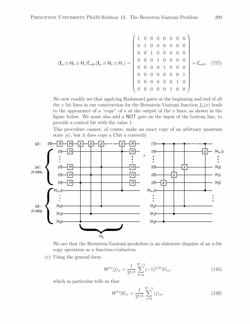
Princeton University Ph410 Solution 13. The Bernstein-Vazirani Problem 209
(Ia ⊗ Hb ⊗ Hc)Cabc(Ia ⊗ Hb ⊗Hc) =
⎛⎜⎜⎜⎜⎜⎜⎜⎜⎜⎜⎜⎜⎜⎜⎜⎜⎜⎜⎝
1 0 0 0 0 0 0 0
0 1 0 0 0 0 0 0
0 0 1 0 0 0 0 0
0 0 0 1 0 0 0 0
0 0 0 0 1 0 0 0
0 0 0 0 0 0 0 1
0 0 0 0 0 0 1 0
0 0 0 0 0 1 0 0
⎞⎟⎟⎟⎟⎟⎟⎟⎟⎟⎟⎟⎟⎟⎟⎟⎟⎟⎟⎠
= Cacb. (757)
We now readily see that applying Hadamard gates at the beginning and end of allthe x bit lines in our construction for the Bernstein-Vazirani function fa(x) leadsto the appearance of a “copy” of a at the output of the x lines, as shown in thefigure below. We must also add a NOT gate on the input of the bottom line, toprovide a control bit with the value 1.
This procedure cannot, of course, make an exact copy of an arbitrary quantumstate |a〉, but it does copy a Cbit a correctly.
We see that the Bernstein-Vazirani prodedure is an elaborate disguise of an n-bitcopy operation as a function evaluation.
(c) Using the general form
H⊗n|j〉n =1
2n/2
2n−1∑k=0
(−1)j�k|k〉n, (145)
which in particular tells us that
H⊗n|0〉n =1
2n/2
2n−1∑j=0
|j〉n, (130)
Princeton University Ph410 Solution 13. The Bernstein-Vazirani Problem 210
along with the relations
Ufa |a〉|x〉|y〉 = |a〉|x〉|y ⊕ fa(x)〉 = |a〉|x〉|y ⊕ (a� x)〉, (166)
and |0 ⊕ f(x)〉 − |1 ⊕ f(x)〉√2
= (−1)f(x) |0〉 − |1〉√2
, (142)
the above bit-flow diagram can be represented algebraically as the sequence ofoperations
(H⊗nx ⊗ Hy)Ufa(H
⊗nx ⊗ HyXy)|0〉x|0〉y = (H⊗n
x ⊗ Hy)Ufa
1
2n/2
2n−1∑j=0
|j〉x( |0〉y − |1〉y√
2
)
= (H⊗nx ⊗ Hy)
1
2n/2
2n−1∑j=0
(−1)fa(j)|j〉x(|0〉y − |1〉y√
2
)
= H⊗nx
1
2n/2
2n−1∑j=0
(−1)a�j|j〉x|1〉y
= H⊗nx H⊗n
x |a〉x|1〉y= |a〉x|1〉y, (758)
noting that H2 = I, so that (H⊗nx )2 = In. Hence, the output lines of |x〉 are in
the desired state |a〉 at the end of the operation, as we also found via the bit-flowdiagram of part (b).
As a side remark, we note that the 3rd and 5th lines of eq. (758) also tell us that
|a〉 = H⊗nx
1
2n/2
2n−1∑j=0
(−1)j�a|j〉n =2n−1∑k=0
1
2n
2n−1∑j=0
(−1)j�k(−1)j�a|k〉n. (759)
Hence, we must have the identity
1
2n
2n−1∑j=0
(−1)j�k(−1)a�j = δak. (168)
To verify this explicitly, we write j =∑n−1l=0 jl2
l where where jl is either 0 or 1.Thus,
1
2n
2n−1∑j=0
(−1)j�k(−1)a�j =1
2n
2n−1∑j=0
(−1)j�(a⊕k) =1
2n
2n−1∑j=0
(−1)∑
ljl(al⊕kl)
=1
2n
2n−1∑j=0
n−1∏l=0
(−1)jl(al⊕kl) =1
2n
n−1∏l=0
1∑jl=0
(−1)jl(al⊕kl). (760)
If k does not equal a then al⊕kl = 1 for a nonzero number of indices l. Whenevernumber j has jl = 1 for exactly one of those indices, the sum in the righthandside of eq. (760) vanishes. Hence, eq. (760) is zero unless a = k, in which case itis equal to 1.

Princeton University Ph410 Solution 14. Simon’s Problem 211
14. Simon’s Problem
(a) We can obtain the value of a from the addition a = x⊕ y once we have found twonumbers x and y such that fa(x) = fa(y). If we pick x and y at random amongthe 2n n-bit numbers, we will need to sample roughly a such pairs to have a goodprobability of finding one pair for which fa(x) = fa(y). Since a is a number oforder 2n, we must make of order 2n evaluations of the function fa to solve theproblem classically.
Therefore, we can say that Simon’s problem is exponentially hard to solve viaclassical computation.
(b) To analyze the operationH⊗nx UfaH
⊗nx |0〉x|0〉y (174)
whereUfa |x〉n|y〉n = |x〉n|y ⊕ fa(x)〉n, (171)
andfa(x) = fa(y) iff y = x⊕ a, (170)
we again use the general form
H⊗n|j〉n =1
2n/2
2n−1∑k=0
(−1)j�k|k〉n, (145)
and its particular case
H⊗n|0〉n =1
2n/2
2n−1∑j=0
|j〉n, (130)
Thus,
H⊗nx UfaH
⊗nx |0〉x|0〉y = H⊗n
x Uf1
2n/2
2n−1∑j=0
|j〉x|0〉y
= H⊗nx
1
2n/2
2n−1∑j=0
|j〉x|fa(j)〉y
= H⊗nx
1
2(n+1)/2
2n−1∑j=0
(|j〉x + |j ⊕ a〉x)|fa(j)〉y (761)
=1
2n+1/2
2n−1∑k=0
2n−1∑j=0
[(−1)j�k + (−1)(j⊕a)�k]|k〉x|fa(j)〉y
=1
2n+1/2
2n−1∑k=0
[1 + (−1)a�k]|k〉x2n−1∑j=0
(−1)j�k|fa(j)〉y,
where we have used the fact that
Ufa
2n−1∑j=0
|j〉n|0〉n =1√2
2n−1∑j=0
(|j〉n + |j ⊕ a〉n)|fa(j)〉n. (173)
in going from the 2nd to the 3rd lines.

Princeton University Ph410 Solution 14. Simon’s Problem 212
We see that the amplitude of a state |k〉n is zero if a�k = 1. Hence, if we measurethe x output lines we find them to have value k only if a� k = 0, and any such kare observed with equal probability. (A measurement of the y output lines is notvery informative.)
If we repeat the process (174) m times, each followed by measurement of the xlines, we build up a set of linear equation
a� kl = 0, l = 1, 2, ..., m, (762)
for the n binary digits of the unknown number a. Not all of these equationsare independent, so in general we need to make m > n repetitions to obtain nindependent (classical) linear equations,165 which we can invert to find a. But therequired number m of repetitions remains of order n, in contrast to the need forof order 2n evaluations of fa to determine a by a classical algorithm.
165 For a discussion of the accuracy to which a can be determined as a function of the number m ofrepetitions, see, for example, sec. IID2 ofhttp://people.ccmr.cornell.edu/~mermin/qcomp/chap2.pdf
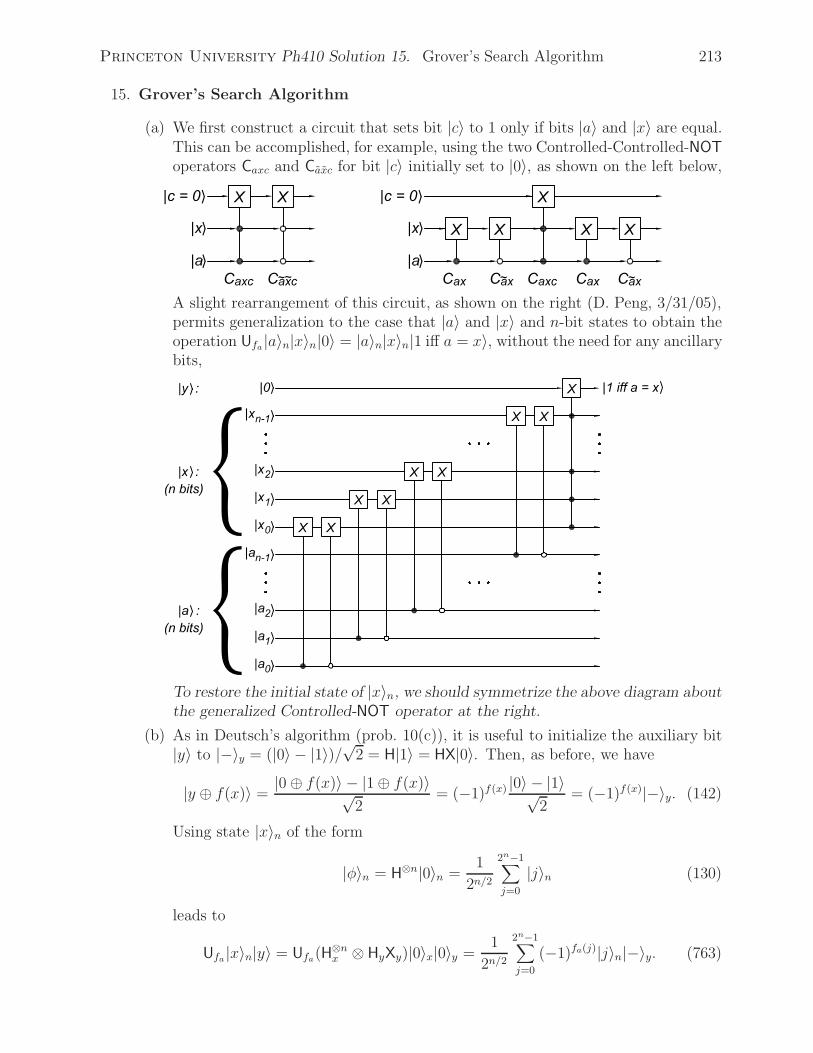
Princeton University Ph410 Solution 15. Grover’s Search Algorithm 213
15. Grover’s Search Algorithm
(a) We first construct a circuit that sets bit |c〉 to 1 only if bits |a〉 and |x〉 are equal.This can be accomplished, for example, using the two Controlled-Controlled-NOToperators Caxc and Caxc for bit |c〉 initially set to |0〉, as shown on the left below,
A slight rearrangement of this circuit, as shown on the right (D. Peng, 3/31/05),permits generalization to the case that |a〉 and |x〉 and n-bit states to obtain theoperation Ufa |a〉n|x〉n|0〉 = |a〉n|x〉n|1 iff a = x〉, without the need for any ancillarybits,
To restore the initial state of |x〉n, we should symmetrize the above diagram aboutthe generalized Controlled-NOT operator at the right.
(b) As in Deutsch’s algorithm (prob. 10(c)), it is useful to initialize the auxiliary bit|y〉 to |−〉y = (|0〉 − |1〉)/√2 = H|1〉 = HX|0〉. Then, as before, we have
|y ⊕ f(x)〉 =|0 ⊕ f(x)〉 − |1 ⊕ f(x)〉√
2= (−1)f(x) |0〉 − |1〉√
2= (−1)f(x)|−〉y. (142)
Using state |x〉n of the form
|φ〉n = H⊗n|0〉n =1
2n/2
2n−1∑j=0
|j〉n (130)
leads to
Ufa |x〉n|y〉 = Ufa(H⊗nx ⊗ HyXy)|0〉x|0〉y =
1
2n/2
2n−1∑j=0
(−1)fa(j)|j〉n|−〉y. (763)
Princeton University Ph410 Solution 15. Grover’s Search Algorithm 214
Since the function fa is
fa(x) =
⎧⎪⎨⎪⎩
0, x = a,
1, x = a., (175)
the amplitude of state |j〉n in eq. (763) is 1/2n/2 unless j = a, in which case theamplitude is −1/2n/2.
Thus we have “marked” the amplitude of the desired state |a〉n differently thanall other (basis) states |j〉n. It remains to find a procedure that can identify the“marked” state efficiently.
(c) The projection of state
|ψ〉n =N−1∑j=0
ψj|j〉n, (182)
onto state
|φ〉n =1√N
N−1∑j=0
|j〉n (130)
is
〈φ|ψ〉n|φ〉n =1√N
N−1∑j=0
ψj|φ〉n =√N⟨ψj⟩|φ〉n =
N−1∑j=0
⟨ψj⟩|j〉n, (764)
where ⟨ψj⟩
=1
N
N−1∑j=0
ψj =1√N〈φ|ψ〉n. (183)
Hence, we can re-express |ψ〉n as
|ψ〉n = 〈φ|ψ〉n|φ〉n + |ψ〉n − 〈φ|ψ〉n|φ〉n=
√N⟨ψj⟩|φ〉n +
N−1∑j=0
(ψj −
⟨ψj⟩)
|j〉n. (765)
The reflection of |ψ〉n about |φ〉n by operator U|φ〉n can now be written as166
U|φ〉n|ψ〉n = 〈φ|ψ〉n|φ〉n − |ψ〉n + 〈φ|ψ〉n|φ〉n = (2|φ〉n〈φ|n − In) |ψ〉n=
√N⟨ψj⟩|φ〉n +
N−1∑j=0
(⟨ψj⟩− ψj
)|j〉n. (766)
Thus, we identify U|φ〉n with the projection operator
U|φ〉n = 2|φ〉n〈φ|n − In, (767)
and we see that its effect is to change the sign of the amplitudes ψj −⟨ψj⟩.
We also get another perspective on Grover’s procedure, in which each interactionconsists of reflecting a state about a plane orthogonal to the desired state |a〉nfollowed by a reflection of all amplitudes about their mean.
166We tacitly assume in eq. (766) that the |y〉 state is |−〉y and remains so under the action of U|φ〉n.
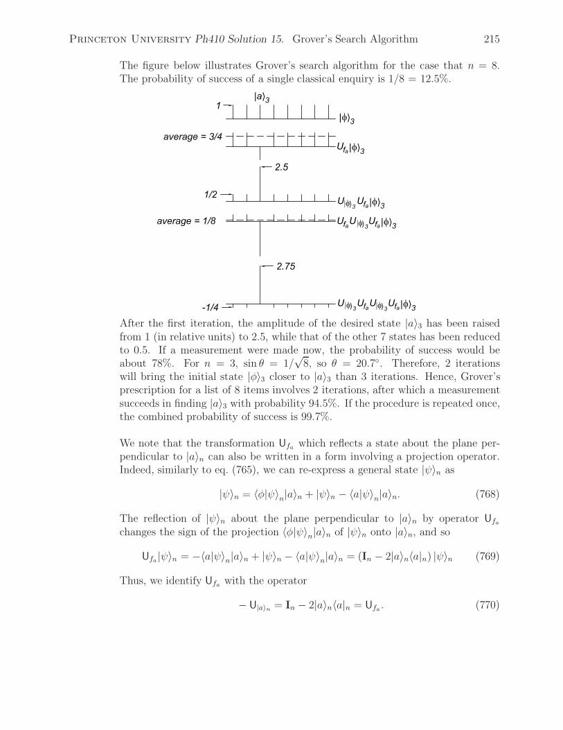
Princeton University Ph410 Solution 15. Grover’s Search Algorithm 215
The figure below illustrates Grover’s search algorithm for the case that n = 8.The probability of success of a single classical enquiry is 1/8 = 12.5%.
After the first iteration, the amplitude of the desired state |a〉3 has been raisedfrom 1 (in relative units) to 2.5, while that of the other 7 states has been reducedto 0.5. If a measurement were made now, the probability of success would beabout 78%. For n = 3, sin θ = 1/
√8, so θ = 20.7◦. Therefore, 2 iterations
will bring the initial state |φ〉3 closer to |a〉3 than 3 iterations. Hence, Grover’sprescription for a list of 8 items involves 2 iterations, after which a measurementsucceeds in finding |a〉3 with probability 94.5%. If the procedure is repeated once,the combined probability of success is 99.7%.
We note that the transformation Ufa which reflects a state about the plane per-pendicular to |a〉n can also be written in a form involving a projection operator.Indeed, similarly to eq. (765), we can re-express a general state |ψ〉n as
|ψ〉n = 〈φ|ψ〉n|a〉n + |ψ〉n − 〈a|ψ〉n|a〉n. (768)
The reflection of |ψ〉n about the plane perpendicular to |a〉n by operator Ufa
changes the sign of the projection 〈φ|ψ〉n|a〉n of |ψ〉n onto |a〉n, and so
Ufa |ψ〉n = −〈a|ψ〉n|a〉n + |ψ〉n − 〈a|ψ〉n|a〉n = (In − 2|a〉n〈a|n) |ψ〉n (769)
Thus, we identify Ufa with the operator
− U|a〉n = In − 2|a〉n〈a|n = Ufa . (770)

Princeton University Ph410 Solution 15. Grover’s Search Algorithm 216
(d) Using the relation|φ〉n = H⊗n|0〉n (130)
and the fact that H = H† = H−1, eq. (767) can be written as167
− U|φ〉n = In − 2|φ〉n〈φ|n = In − 2H⊗n|0〉n〈0|nH⊗n
= H⊗n(In − 2|0〉n〈0|n)H⊗n = −H⊗nU|0〉nH⊗n
= H⊗nUf0H⊗n. (771)
Recalling our construction of Ufa in part (a), we can implement Uf0 = −U|0〉naccording to eq. (771) as shown below, deleting the unnecessary lines for |a〉n =|0〉n,
Note that for the above circuit to change the sign of the amplitude of |0〉x (andthat of no other basis state |j〉x), the auxiliary bit |y〉 must be prepared in thestate HX|0〉y = |−〉y. If we use the same bit |y〉 for this purpose as was used inthe operation Ufa , that bit is already in the needed state, so we don’t add anynew gates for this purpose to our construction of Uf0 .
168
Our prescription for the m iterations of Grover’s search algorithm can now besummarized as
[(H⊗nx ⊗ Iy)U|0〉n(H⊗n
x ⊗ Iy)Ufa ]m(H⊗n
x ⊗ HyXy)|0〉x|0〉y . (772)
To use the same n auxiliary lines in all operators Ufa , the construction given inpart (a) must be symmetrized. If bits are cheaper than gates, it might be simplerto introduce a new set of n auxiliary bits for each Ufa to reduce the overall numberof gates.
167Again, the |y〉 state is to be |−〉y before and after the operation U|φ〉n.
168Most texts seem to consider the bit |y〉 needed for Uf0 as different from the bit |y〉 needed for Ufa. Then,they note the appearance of the product HyXyHy on the |y〉 line in Uf0 . Since this product equals Z = σz,one often sees diagrams with Controlled-Z operations describing Grover’s algorithm.

Princeton University Ph410 Solution 16. Parity of a Function 217
16. Parity of a Function
A single application of the circuit yields
(H⊗nx ⊗ XyHy)Uf (H
⊗nx ⊗ HyXy)|0〉x|0〉y =
1
2n
2n−1∑j=0
2n−1∑k=0
(−1)f(j)(−1)j�k|k〉n|0〉y, (773)
using eqs. (130), (142), (145) and (186).
For the case that n = 1, the righthand side of eq. (773) is
1
2
{(−1)f(0)[(−1)0�0|0〉 + (−1)0�1|1〉] + (−1)f(1)[(−1)1�0|0〉 + (−1)1�1|1〉]
}
=(−1)f(0)
2
{[(−1)0|0〉 + (−1)0|1〉] + Πf [(−1)0|0〉 + (−1)1|1〉]
}
=(−1)f(0)
2[(1 + Πf)|0〉 + (1 − Πf)|1〉], (774)
using the fact that
(−1)f(1) = (−1)f(0)(−1)f(1)−f(0) = (−1)f(0)(−1)f(1)+f(0) = (−1)f(0)Πf , (187)
since f = 0 or 1 only.
Thus, a measurement of the righthand side of eq. (773) yields the state |0〉 if Πf = 1and |1〉 if Πf = −1.
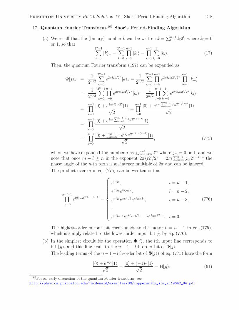
Princeton University Ph410 Solution 17. Shor’s Period-Finding Algorithm 218
17. Quantum Fourier Transform,169 Shor’s Period-Finding Algorithm
(a) We recall that the (binary) number k can be written k =∑n−1l=0 kl2
l, where kl = 0or 1, so that
2n−1∑k=0
|k〉n =2n−1∑k=0
n−1∏l=0
|kl〉 =n−1∏l=0
1∑kl=0
|kl〉. (17)
Then, the quantum Fourier transform (197) can be expanded as
Φ|j〉n =1
2n/2
2n−1∑k=0
e2πijk/2n|k〉n =1
2n/2
2n−1∑k=0
n−1∏l=0
e2πijkl2l/2n
n−1∏m=0
|km〉
=1
2n/2
2n−1∑k=0
n−1∏l=0
e2πijkl2l/2n|kl〉 =
1
2n/2
n−1∏l=0
1∑kl=0
e2πijkl2l/2n|kl〉
=n−1∏l=0
|0〉 + e2πij2l/2n|1〉√2
=n−1∏l=0
|0〉 + e2πi∑n−1
m=0jm2m2l/2n|1〉√
2
=n−1∏l=0
|0〉 + e2πi∑n−l−1
m=0jm2m+l−n |1〉√
2
=n−1∏l=0
|0〉 +∏n−l−1m=0 eπijm2m+l−(n−1) |1〉√
2, (775)
where we have expanded the number j as∑n−1m=0 jm2m where jm = 0 or 1, and we
note that once m + l ≥ n in the exponent 2πij2l/2n = 2πi∑n−1m=0 jm2m+l−n the
phase angle of the mth term is an integer multiple of 2π and can be ignored.
The product over m in eq. (775) can be written out as
n−l−1∏m=0
eπijm2m+l−(n−1)
=
⎧⎪⎪⎪⎪⎪⎪⎪⎪⎪⎪⎪⎪⎨⎪⎪⎪⎪⎪⎪⎪⎪⎪⎪⎪⎪⎩
eπij0 , l = n − 1,
eπij1eπij0/2, l = n − 2,
eπij2eπij1/2eπij0/22, l = n − 3,
...
eπijn−1eπijn−2/2 · · · eπij0/2n−1, l = 0.
(776)
The highest-order output bit corresponds to the factor l = n − 1 in eq. (775),which is simply related to the lowest-order input bit j0 by eq. (776).
(b) In the simplest circuit for the operation Φ|j〉, the lth input line corresponds tobit |jl〉, and this line leads to the n− 1 − lth-order bit of Φ|j〉.The leading terms of the n− 1− lth-order bit of Φ|j〉) of eq. (775) have the form
|0〉 + eπijl |1〉√2
=|0〉 + (−1)jl|1〉√
2= H|jl〉. (61)
169For an early discussion of the quantum Fourier transform, seehttp://physics.princeton.edu/~mcdonald/examples/QM/coppersmith_ibm_rc19642_94.pdf

Princeton University Ph410 Solution 17. Shor’s Period-Finding Algorithm 219
An additional factor of eπi/2n−1−l−m
= (−1)1/2n−1−l−mmultiples the |1〉 in the lth
factor whenever |jm〉 = |1〉 for 0 ≤ m < n − 1 − l. This suggests use of anoperation that affects only the |1〉 state of bit l whenever bit m is 1, i.e., somekind of Controlled operation Uml. We readily see that the desired operation isU = Z1/2n−1−l−m
= (σ1/4z )1/2n−l−m−3
.
Putting together these pieces, we apply the Hadamard transformation to inputline l only after the state of that line has been used to generate the needed phasefactors for lines m > l. Hence, we can represent the quantum Fourier transformΦ|j〉n as
The above diagram can be drawn slightly differently by noting a property ofControlled-Zp that arises because the only effect of Zp is to change the phase ofthe |1〉 state. Since
Zp =
⎛⎝ 1 0
0 eπip
⎞⎠ , (777)
the 2-Qbit Controlled-Zp matrix has the form
Zpab =
⎛⎜⎜⎜⎜⎜⎜⎝
1 0 0 0
0 1 0 0
0 0 1 0
0 0 0 eπip
⎞⎟⎟⎟⎟⎟⎟⎠
= Zpba.
(778)Thus, there is actually no distinction between the control and target bits of aControlled-Zp gate. Hence, the quantum Fourier transform Φ can also be repre-sented as
There is no hardware difference between this diagram and the previous; the dif-ference is only one of notation.
(c) Recalling the definition (194) of the discrete Fourier transform, we see that theinverse Fourier transform is the same as the Fourier transform except for thereversal of the signs of all the phases in the exponential phase factors. Hence, the

Princeton University Ph410 Solution 17. Shor’s Period-Finding Algorithm 220
inverse form of eq. (197) is
Φ−1|j〉n =1
2n/2
2n−1∑k=0
e−2πijk/2n|k〉n. (779)
Rearranging this in the fashion of eq. (775), we have
Φ−1|j〉n =n−1∏l=0
|0〉 +∏n−l−1m=0 e−πijm2m+l−(n−1) |1〉√
2. (780)
A bit-flow diagram corresponding to eq. (780) is
Although Z−1 = Z, in general Z−p = Zp. Hence, the circuit for the inverse Fouriertransform Φ−1 is distinct from that for the Fourier transform Φ.
(d) Period Finding.
Applying the quantum Fourier transform,
Φ|j〉n =1
2n/2
2n−1∑k=0
e2πijk/2n|k〉n, (197)
to the state (202) and noting that ab ≈ 2n, we have
ΦxUfH⊗nx |0〉x|0〉y = Φx
1√a
a−1∑j=0
1√b
b−1∑m=0
|j +ma〉x|f(j)〉y
=1√a
a−1∑j=0
1√b
b−1∑m=0
1
2n/2
2n−1∑k=0
e2πi(j+ma)k/2n|k〉x|f(j)〉y
=1√ab2n
2n−1∑k=0
a−1∑j=0
e2πijk/2nb−1∑m=0
e2πimak/2n|k〉x|f(j)〉y
=1
2n
2n−1∑k=0
a−1∑j=0
e2πijk/2nb−1∑m=0
(e2πiak/2n
)m|k〉x|f(j)〉y
=1
2n
2n−1∑k=0
a−1∑j=0
e2πijk/2n 1 − e2πiabk/2n
1 − e2πiak/2n |k〉x|f(j)〉y
=1
2n
2n−1∑k=0
a−1∑j=0
e2πijk/2n eπiabk/2n
eπiak/2n
sin(πabk/2n)
sin(πak/2n)|k〉x|f(j)〉y
≈ 1
2n
2n−1∑k=0
a−1∑j=0
eiφjksin(πk)
sin(πak/2n)|k〉x|f(j)〉y, (781)
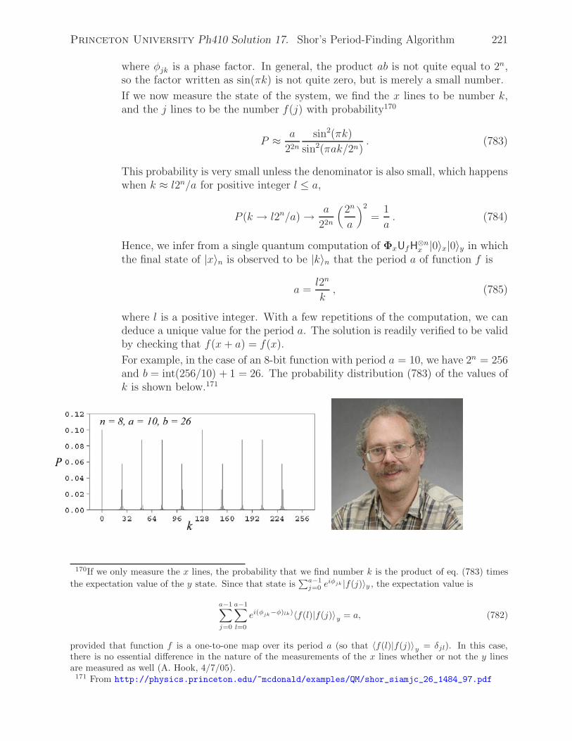
Princeton University Ph410 Solution 17. Shor’s Period-Finding Algorithm 221
where φjk is a phase factor. In general, the product ab is not quite equal to 2n,so the factor written as sin(πk) is not quite zero, but is merely a small number.
If we now measure the state of the system, we find the x lines to be number k,and the j lines to be the number f(j) with probability170
P ≈ a
22n
sin2(πk)
sin2(πak/2n). (783)
This probability is very small unless the denominator is also small, which happenswhen k ≈ l2n/a for positive integer l ≤ a,
P (k → l2n/a) → a
22n
(2n
a
)2
=1
a. (784)
Hence, we infer from a single quantum computation of ΦxUfH⊗nx |0〉x|0〉y in which
the final state of |x〉n is observed to be |k〉n that the period a of function f is
a =l2n
k, (785)
where l is a positive integer. With a few repetitions of the computation, we candeduce a unique value for the period a. The solution is readily verified to be validby checking that f(x+ a) = f(x).
For example, in the case of an 8-bit function with period a = 10, we have 2n = 256and b = int(256/10) + 1 = 26. The probability distribution (783) of the values ofk is shown below.171
170If we only measure the x lines, the probability that we find number k is the product of eq. (783) timesthe expectation value of the y state. Since that state is
∑a−1j=0 e
iφjk |f(j)〉y , the expectation value is
a−1∑j=0
a−1∑l=0
ei(φjk−φ)lk)〈f(l)|f(j)〉y = a, (782)
provided that function f is a one-to-one map over its period a (so that 〈f(l)|f(j)〉y = δjl). In this case,there is no essential difference in the nature of the measurements of the x lines whether or not the y linesare measured as well (A. Hook, 4/7/05).
171 From http://physics.princeton.edu/~mcdonald/examples/QM/shor_siamjc_26_1484_97.pdf
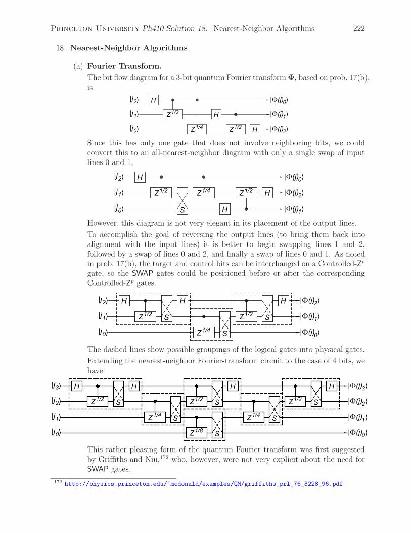
Princeton University Ph410 Solution 18. Nearest-Neighbor Algorithms 222
18. Nearest-Neighbor Algorithms
(a) Fourier Transform.
The bit flow diagram for a 3-bit quantum Fourier transform Φ, based on prob. 17(b),is
Since this has only one gate that does not involve neighboring bits, we couldconvert this to an all-nearest-neighbor diagram with only a single swap of inputlines 0 and 1,
However, this diagram is not very elegant in its placement of the output lines.
To accomplish the goal of reversing the output lines (to bring them back intoalignment with the input lines) it is better to begin swapping lines 1 and 2,followed by a swap of lines 0 and 2, and finally a swap of lines 0 and 1. As notedin prob. 17(b), the target and control bits can be interchanged on a Controlled-Zp
gate, so the SWAP gates could be positioned before or after the correspondingControlled-Zp gates.
The dashed lines show possible groupings of the logical gates into physical gates.
Extending the nearest-neighbor Fourier-transform circuit to the case of 4 bits, wehave
This rather pleasing form of the quantum Fourier transform was first suggestedby Griffiths and Niu,172 who, however, were not very explicit about the need forSWAP gates.
172 http://physics.princeton.edu/~mcdonald/examples/QM/griffiths_prl_76_3228_96.pdf

Princeton University Ph410 Solution 18. Nearest-Neighbor Algorithms 223
Although the nearest-neighbor Fourier transform circuit appears to be left-rightsymmetric, this does not imply that the Fourier transform is its own inverse. Notethat input line j connects with output line n−j−1, so the symmetry of the circuitis only partial.
(b) Fourier Addition.
Recalling, eq. (775), we can expand the quantum Fourier transform of two (n−1)-bit numbers a and b as
Φ|a + b〉n =n−1∏l=0
|0〉 +∏n−l−1m=0 eπi(a+b)m2m+l−(n−1)|1〉√
2
=n−1∏l=0
|0〉 +∏n−l−1k=0 eπiak2k+l−(n−1) ∏n−l−1
m=0 eπibm2m+l−(n−1) |1〉√2
=n−1∏l=0
|0〉 +∏n−l−1k=0
(Z2k+l−(n−1)
)ak ∏n−l−1m=0 eπibm2m+l−(n−1) |1〉√
2
=n−1∏l=0
n−l−1∏k=0
(Z2k+l−(n−1)
)ak |0〉 +∏n−l−1m=0 eπibm2m+l−(n−1) |1〉√
2
=n−1∏l=0
n−l−1∏k=0
(Z2k+l−(n−1)
)ak |Φ(b)m〉n ≡ Φ+a (b), (786)
noting that any power of the operator Z has no effect on the state |0〉. This tellsus that the lth bit of Φ|a+ b〉n is the lth bit of Φ|b〉n after it has been acted upon
by the operator product∏n−l−1k=0
(Z2k+l−(n−1)
)akbased on number a =
∑n−1k=0 ak2
k.Implementing these factor is very similar to the task of implementing the originalFourier transform, with the simplification that the H gates are just Z gates now.
A general bit-flow diagram for the Fourier addition |Φ(a + b)n〉 is thus
Since number a actually has only n − 1 bits, the line labeled |an−1〉 can be elim-inated. Note, however, that the n-bit Fourier transform |Φ(b)〉n has nontrivialstructure on all of its n lines.
Note also that since the Controlled-Zp gates commute with one another, the gatesin the above circuit could be applied in any order.
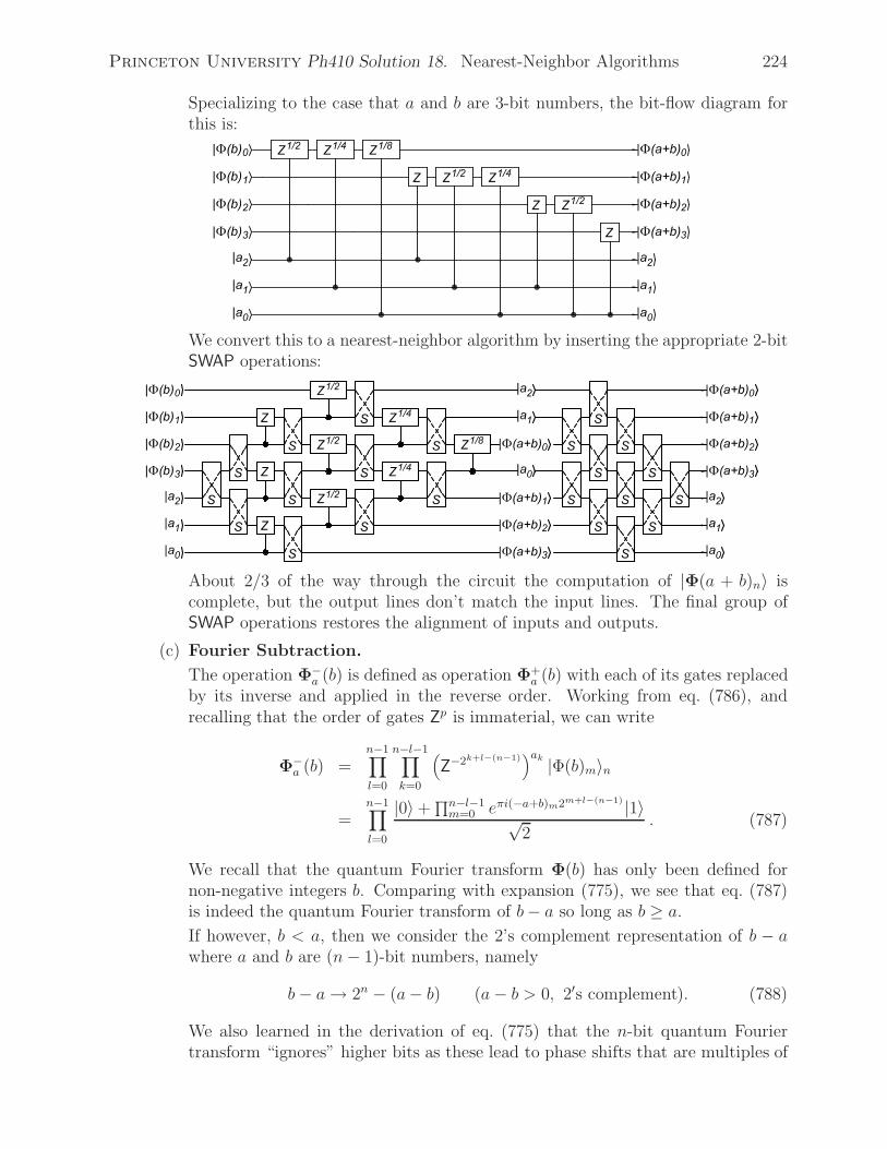
Princeton University Ph410 Solution 18. Nearest-Neighbor Algorithms 224
Specializing to the case that a and b are 3-bit numbers, the bit-flow diagram forthis is:
We convert this to a nearest-neighbor algorithm by inserting the appropriate 2-bitSWAP operations:
About 2/3 of the way through the circuit the computation of |Φ(a + b)n〉 iscomplete, but the output lines don’t match the input lines. The final group ofSWAP operations restores the alignment of inputs and outputs.
(c) Fourier Subtraction.
The operation Φ−a (b) is defined as operation Φ+
a (b) with each of its gates replacedby its inverse and applied in the reverse order. Working from eq. (786), andrecalling that the order of gates Zp is immaterial, we can write
Φ−a (b) =
n−1∏l=0
n−l−1∏k=0
(Z−2k+l−(n−1)
)ak |Φ(b)m〉n
=n−1∏l=0
|0〉 +∏n−l−1m=0 eπi(−a+b)m2m+l−(n−1) |1〉√
2. (787)
We recall that the quantum Fourier transform Φ(b) has only been defined fornon-negative integers b. Comparing with expansion (775), we see that eq. (787)is indeed the quantum Fourier transform of b− a so long as b ≥ a.
If however, b < a, then we consider the 2’s complement representation of b − awhere a and b are (n− 1)-bit numbers, namely
b− a→ 2n − (a− b) (a− b > 0, 2′s complement). (788)
We also learned in the derivation of eq. (775) that the n-bit quantum Fouriertransform “ignores” higher bits as these lead to phase shifts that are multiples of

Princeton University Ph410 Solution 18. Nearest-Neighbor Algorithms 225
2π. Thus, the quantum Fourier subtraction operator Φ−a (b) “naturally” performs
2’s complement subtraction.
(d) Controlled Fourier Addition.
The circuit for a Controlled-Controlled-U2 operation that was given in prob. 11(c)becomes a nearest-neighbor algorithm with the addition of two SWAP gates:
To implement a Controlled-Fourier addition using Controlled-Controlled-Zp gates,I found it convenient to group together all such operations on a given bit of Φ(b).Also, it seemed simplest if the control bit |c〉 is between |a〉 and |Φ(b)〉, and theorder of the bits of |a〉 is reversed (otherwise 6 more layers of SWAP gates arerequired):

Princeton University Ph410 Solution 19. Spin Control 226
19. Spin Control
(a) Single-Qbit Gates via Pulsed Magnetic Fields
We wish to evaluate the rotating-frame Hamiltonian,
hrot = e−iω0t
2σz
(hlab +
ω0
2σz
)ei
ω0t
2σz (236)
for a spin-1/2 particle at rest in the time-dependent magnetic field
B = B0z+Bu[ux(cosω0t x− sinω0t y)+uy(sinω0t x+cosω0t y)+uz z]. (237)
The lab-frame (reduced) interaction Hamiltonian hlab = H/h for a spin-1/2 par-ticle with magnetic moment μ = γs = hΓσ/2 in the magnetic field (237) is givenby
hlab = −Γ
2σ · B = −ΓB0
2σz
−ΓBu
2[ux(cosω0t σx − sinω0t σy) + uy(sinω0t σx + cosω0t σy) + uz σz]
= −ω0
2σz (789)
−ωu2
[(ux cosω0t+ uy sinω0t)σx + (−ux sinω0t+ uy cosω0t)σy + uzσz]
where ω0 = ΓB0 and ωu = ΓBu. On using this in eq. (236), we need to evaluatethe products
e−iω0t2
σzσjei
ω0t2
σz =(cos
ω0t
2I − i sin
ω0t
2σz
)σj
(cos
ω0t
2I + i sin
ω0t
2σz
)
= cos2 ω0t
2σj − i cos
ω0t
2sin
ω0t
2(σzσj − σjσz) + sin2 ω0t
2σzσjσz
=
⎧⎪⎪⎪⎪⎪⎨⎪⎪⎪⎪⎪⎩
cosω0t σx + sinω0t σy (j = x),
− sinω0t σx + cosω0t σy (j = y),
σz (j = z).
(790)
Combining eqs. (236), (789) and (790), we find the Hamiltonian in the rotatingframe to be
hrot = −ωu2
u · σ. (791)
If the lab-frame magnetic field is
B = B0z +Bx(cosωt x − sinωt y), (240),
then the (reduced) lab-frame interaction Hamiltonian is
hlab = −Γ
2σ · B = −ΓB0
2σz − ΓBx
2(cosωt σx − sinωt σy)
= −ω0
2σz − ωx
2(cosωt σx − sinωt σy)
= −ω0
2σz − ωx
2
(eiωt
σx + iσy2
+ e−iωtσx − iσy
2
)
= −ω0
2σz − ωx
2
(eiωta† + e−iωta
), (792)

Princeton University Ph410 Solution 19. Spin Control 227
where ωx = ΓBx, and
a =σx − iσy
2=
⎛⎝ 0 1
0 0
⎞⎠ , and a† =
σx + iσy2
=
⎛⎝ 0 0
1 0
⎞⎠ (793)
are the annihilation and creation operators introduced in prob. 9. We could alsouse eqs. (123) and (125) to write σz = aa†− a†a to express the Hamiltonian (792)entirely in terms of annihilation and creation operators, but this is not reallynecessary.
Then, inserting the trial solution
|ψ(t)〉 = Aeiαt|0〉 +Be−iβt|1〉 (241)
into Schrodinger’s equation, i∂t|ψ〉 = hlab|ψ〉, usinig eq. (792) we find (for thecoefficients of |0〉 and |1〉)
− αAeiαt = −ω0
2Aeiαt − ωx
2eiωtBe−iβt, (794)
βBe−iβt =ω0
2Be−iβt − ωx
2e−iωtAeiαt, (795)
or
α =ω0
2+ωx2
B
Ae−i(α+β−ω)t, (796)
β =ω0
2− ωx
2
A
Bei(α+β−ω)t. (797)
These equations can only be satisfied if
α+ β = ω, (798)
in which case eqs. (796)-(797) become
α =ω0
2+ωx2
B
A, (799)
β =ω0
2− ωx
2
A
B. (800)
Substituting eqs. (799)-(800) into eq. (798), we have
ω0 +ωx2
B
A− ωx
2
A
B− ω = 0, (801)
A
B− 2
ω0 − ω
ωx− B
A= 0, (802)
A2
B2− 2
ω0 − ω
ωx
A
B− 1 = 0 =
B2
A2+ 2
ω0 − ω
ωx
B
A− 1, (803)
A
B=ω0 − ω ±
√(ω0 − ω)2 + ω2
x
ωx, (804)
Princeton University Ph410 Solution 19. Spin Control 228
B
A=ω − ω0 ±
√(ω0 − ω)2 + ω2
x
ωx, (805)
α =ω0
2+ωx2
B
A=ω ∓
√(ω0 − ω)2 + ω2
x
2, (806)
β =ω0
2− ωx
2
A
B=ω ±
√(ω0 − ω)2 + ω2
x
2, (807)
and indeed,α+ β = ω. (798)
We have found two solutions, which must be added to give the general solutionto Schrodinger’s equation.
We defineΩ =
√(ω0 − ω)2 + ω2
x, (808)
so that the time-dependent Qbit (241) has the general form
|ψ(t)lab〉 = (A1e−iΩt + A2e
iΩt)eiω2t|0〉 + (B1e
iΩt +B2e−iΩt)e−i
ω2t|1〉. (809)
The coefficients Aj and Bj are related according to eq. (804),
A1 =ω0 − ω + Ω
ωxB1, A2 =
ω0 − ω − Ω
ωxB2. (810)
If the initial Qbit is |ψ(0)〉 = a|0〉 + b|1〉, then eq. (809) tells us that
A1 + A2 = a, B1 +B2 = b. (811)
Substituting eq. (810) into the first equation of (811), and then using the secondequation of (811) to eliminate for B2, we have
ω0 − ω + Ω
ωxB1 +
ω0 − ω − Ω
ωx(b− B1) = a, (812)
2Ω
ωxB1 = a− ω0 − ω − Ω
ωxb, (813)
B1 =ωx2Ω
a− ω0 − ω − Ω
2Ωb, (814)
A1 =ω0 − ω + Ω
ωxB1 =
ω0 − ω + Ω
2Ωa− (ω0 − ω)2 − Ω2
2ωxΩb, (815)
B2 = b− B1 = −ωx2Ω
a+ω0 − ω + Ω
2Ωb, (816)
A2 =ω0 − ω − Ω
ωxB2 = −ω0 − ω − Ω
2Ωa +
(ω0 − ω)2 − Ω2
2ωxΩb. (817)
Princeton University Ph410 Solution 19. Spin Control 229
Using eqs. (814)-(817) in eq. (809), we have
|ψ(t)lab〉 =
{a cosΩt+ i
[−ω0 − ω
Ωa +
(ω0 − ω)2 − Ω2
ωxΩb
]sin Ωt
}ei
ω2t|0〉
+{i[ωxΩa− ω0 − ω
Ωb]sinΩt+ b cos Ωt
}e−i
ω2t|1〉. (818)
In particular, if |ψ(0)〉 = |0〉, then
|ψ(t)lab〉 =(cos Ωt− i
ω0 − ω
ΩsinΩt
)ei
ω2t|0〉 + i
ωxΩ
sinΩte−iω2t|1〉. (819)
If in addition the frequency ω of the oscillatory field Bx is equal to the Larmorfrequency ω0 that corresponds to the spin-flip energy, then
Ω = ωx (ω0 = ω), (820)
and the time dependence of the Qbit is
|ψ(t)lab〉 = cosωxtei
ω02t|0〉 + i sinωxte
−iω02t|1〉 (ω0 = ω, |ψ(0)〉 = |0〉), (821)
which is commonly called spin resonance or magnetic resonance. Similarly, in thecase of spin resonance when the initial state of the Qbit is |1〉, we have
|ψ(t)lab〉 = −i sinωxteiω02t|0〉+cosωxte
−iω02t|1〉 (ω0 = ω, |ψ(0)〉 = |1〉). (822)
If the oscillatory field Bx is applied for a time t such that ωxt = π/2, thenthere is 100% probability that the Qbit state will have been flipped. That is, aNOT operation (up to a phase) for spin-based Qbits consists of application of atransverse magnetic field of frequency ω0 for 1/4 of the Rabi period, i.e., for timet = π/2ωx.
(b) Two-Bit Coupling
We wish to ascertain the character of the unitary transformation U12 that char-acterizes the time evolution over a period t = π/2ω12 of two spin-based Qbits (asviewed in their respective rotating frames) whose (lab-frame) interaction Hamil-tonian is
h12 =ω12
2σ(1) ·σ(2). (244)
We have that
|ψ′rot〉12 = e−i
ω12t2
σ(1)x σ
(2)x e−i
ω12t2
σ(1)y σ
(2)y e−i
ω12t2
σ(1)z ·σ(2)
z |ψrot〉12 = U12|ψrot〉12. (245)
Sincee−iασ
(1)j σ
(2)j = cosα I − i sinα σ
(1)j σ
(2)j , (823)
where α = ω12t/2 = π/4 in the present case, we need to evaluate the operation
(I − iσ(1)j σ
(2)j )/
√2 for j = x, y, z. Recalling eq. (647) for the tensor product of
two 2-Qbit operations, we have
σ(1)x σ
(2)x =
⎛⎜⎝ 0 σx
σx 0
⎞⎟⎠ =
⎛⎜⎜⎜⎜⎜⎜⎝
0 0 0 1
0 0 1 0
0 1 0 0
1 0 0 0
⎞⎟⎟⎟⎟⎟⎟⎠, (824)

Princeton University Ph410 Solution 19. Spin Control 230
and so
e−iπ4σ
(1)x σ
(2)x =
1√2
⎛⎜⎜⎜⎜⎜⎜⎝
1 0 0 −i0 1 −i 0
0 −i 1 0
−i 0 0 1
⎞⎟⎟⎟⎟⎟⎟⎠. (825)
Similarly,
σ(1)y σ
(2)y =
⎛⎜⎝ 0 −iσyiσy 0
⎞⎟⎠ =
⎛⎜⎜⎜⎜⎜⎜⎝
0 0 0 −1
0 0 1 0
0 1 0 0
−1 0 0 0
⎞⎟⎟⎟⎟⎟⎟⎠, (826)
e−iπ4σ
(1)y σ
(2)y =
1√2
⎛⎜⎜⎜⎜⎜⎜⎝
1 0 0 i
0 1 −i 0
0 −i 1 0
i 0 0 1
⎞⎟⎟⎟⎟⎟⎟⎠, (827)
σ(1)z σ
(2)z =
⎛⎜⎝ σz 0
0 −σz
⎞⎟⎠ =
⎛⎜⎜⎜⎜⎜⎜⎝
1 0 0 0
0 −1 0 0
0 0 −1 0
0 0 0 1
⎞⎟⎟⎟⎟⎟⎟⎠, (828)
and
e−iπ4σ
(1)z σ
(2)z =
1√2
⎛⎜⎜⎜⎜⎜⎜⎝
1 − i 0 0 0
0 1 + i 0 0
0 0 1 + i 0
0 0 0 1 − i
⎞⎟⎟⎟⎟⎟⎟⎠. (829)
Then,
e−iπ4σ
(1)x σ
(2)x e−i
π4σ
(1)y σ
(2)y =
1
2
⎛⎜⎜⎜⎜⎜⎜⎝
1 0 0 −i0 1 −i 0
0 −i 1 0
−i 0 0 1
⎞⎟⎟⎟⎟⎟⎟⎠
⎛⎜⎜⎜⎜⎜⎜⎝
1 0 0 i
0 1 −i 0
0 −i 1 0
i 0 0 1
⎞⎟⎟⎟⎟⎟⎟⎠
=
⎛⎜⎜⎜⎜⎜⎜⎝
1 0 0 0
0 0 −i 0
0 −i 0 0
0 0 0 1
⎞⎟⎟⎟⎟⎟⎟⎠. (830)
This is almost the swap operation (572), except for the phase change between theswaps |0〉|0〉 ↔ |1〉|1〉 and the swaps |0〉|1〉 ↔ |1〉|0〉. This discrepancy is fixed by

Princeton University Ph410 Solution 19. Spin Control 231
the operator e−iπ4σ
(1)z σ
(2)z :
e−iπ4σ
(1)x σ
(2)x e−i
π4σ
(1)y σ
(2)y e−i
π4σ
(1)z σ
(2)z =
1√2
⎛⎜⎜⎜⎜⎜⎜⎝
1 0 0 0
0 0 −i 0
0 −i 0 0
0 0 0 1
⎞⎟⎟⎟⎟⎟⎟⎠
⎛⎜⎜⎜⎜⎜⎜⎝
1 − i 0 0 0
0 1 + i 0 0
0 0 1 + i 0
0 0 0 1 − i
⎞⎟⎟⎟⎟⎟⎟⎠
=1 − i√
2
⎛⎜⎜⎜⎜⎜⎜⎝
1 0 0 0
0 0 1 0
0 1 0 0
0 0 0 1
⎞⎟⎟⎟⎟⎟⎟⎠
=1 − i√
2S12. (831)
To show thatC12 = e−i
π4σ
(1)z ei
π4σ
(2)y ei
π4σ
(2)z e−i
π4σ
(1)z σ
(2)z e−i
π4σ
(2)y , (247)
we accumulate the 4 × 4 matrix representations of the various operators. Thus,
e±iπ4σ
(2)y =
I ± iI(1)σ(2)y√
2=
1√2
⎛⎜⎜⎜⎜⎜⎜⎝
1 ±1 0 0
∓1 1 0 0
0 0 1 ±1
0 0 ∓1 1
⎞⎟⎟⎟⎟⎟⎟⎠, (832)
e−iπ4σ
(1)z =
I − iσ(1)z I(2)
√2
=1√2
⎛⎜⎜⎜⎜⎜⎜⎝
1 − i 0 0 0
0 1 − i 0 0
0 0 1 + i 0
0 0 0 1 + i
⎞⎟⎟⎟⎟⎟⎟⎠, (833)
and
eiπ4σ
(2)z =
I + iI(1)σ(2)z√
2=
1√2
⎛⎜⎜⎜⎜⎜⎜⎝
1 + i 0 0 0
0 1 − i 0 0
0 0 1 + i 0
0 0 0 1 − i
⎞⎟⎟⎟⎟⎟⎟⎠. (834)
Then,
e−iπ4σ
(1)z ei
π4σ
(2)y ei
π4σ
(2)z e−i
π4σ
(1)z σ
(2)z e−i
π4σ
(2)y
=1
2e−i
π4σ
(1)z ei
π4σ
(2)y ei
π4σ
(2)z
⎛⎜⎜⎜⎜⎜⎜⎝
1 − i 0 0 0
0 1 + i 0 0
0 0 1 + i 0
0 0 0 1 − i
⎞⎟⎟⎟⎟⎟⎟⎠
⎛⎜⎜⎜⎜⎜⎜⎝
1 −1 0 0
1 1 0 0
0 0 1 −1
0 0 1 1
⎞⎟⎟⎟⎟⎟⎟⎠

Princeton University Ph410 Solution 19. Spin Control 232
=1
2√
2e−i
π4σ
(1)z ei
π4σ
(2)y
⎛⎜⎜⎜⎜⎜⎜⎝
1 + i 0 0 0
0 1 − i 0 0
0 0 1 + i 0
0 0 0 1 − i
⎞⎟⎟⎟⎟⎟⎟⎠
⎛⎜⎜⎜⎜⎜⎜⎝
1 − i −1 + i 0 0
1 + i 1 + i 0 0
0 0 1 + i −1 − i
0 0 1 − i 1 − i
⎞⎟⎟⎟⎟⎟⎟⎠
=1
2e−i
π4σ
(1)z
⎛⎜⎜⎜⎜⎜⎜⎝
1 1 0 0
−1 1 0 0
0 0 1 1
0 0 −1 1
⎞⎟⎟⎟⎟⎟⎟⎠
⎛⎜⎜⎜⎜⎜⎜⎝
1 −1 0 0
1 1 0 0
0 0 i −i0 0 −i −i
⎞⎟⎟⎟⎟⎟⎟⎠
=1√2
⎛⎜⎜⎜⎜⎜⎜⎝
1 − i 0 0 0
0 1 − i 0 0
0 0 1 + i 0
0 0 0 1 + i
⎞⎟⎟⎟⎟⎟⎟⎠
⎛⎜⎜⎜⎜⎜⎜⎝
1 0 0 0
0 1 0 0
0 0 0 −i0 0 −i 0
⎞⎟⎟⎟⎟⎟⎟⎠
=1 − i√
2
⎛⎜⎜⎜⎜⎜⎜⎝
1 0 0 0
0 1 0 0
0 0 0 1
0 0 1 0
⎞⎟⎟⎟⎟⎟⎟⎠
=1 − i√
2C12. (835)
To verify that
C21 = e−iπ4σ
(2)z ei
π4σ
(1)y ei
π4σ
(1)z e−i
π4σ
(1)z σ
(2)z e−i
π4σ
(1)y , (248)
we note that
e±iπ4σ
(1)y =
I ± iσ(1)y I(2)
√2
=1√2
⎛⎜⎜⎜⎜⎜⎜⎝
1 0 ±1 0
0 1 0 ±1
∓1 0 1 0
0 ∓1 0 1
⎞⎟⎟⎟⎟⎟⎟⎠, (836)
eiπ4σ
(1)z =
I + iσ(1)z I(2)
√2
=1√2
⎛⎜⎜⎜⎜⎜⎜⎝
1 + i 0 0 0
0 1 + i 0 0
0 0 1 − i 0
0 0 0 1 − i
⎞⎟⎟⎟⎟⎟⎟⎠, (837)
and
e−iπ4σ
(2)z =
I − iI(1)σ(2)z√
2=
1√2
⎛⎜⎜⎜⎜⎜⎜⎝
1 − i 0 0 0
0 1 + i 0 0
0 0 1 − i 0
0 0 0 1 + i
⎞⎟⎟⎟⎟⎟⎟⎠. (838)

Princeton University Ph410 Solution 19. Spin Control 233
Then,
e−iπ4σ
(2)z ei
π4σ
(1)y ei
π4σ
(1)z e−i
π4σ
(1)z σ
(2)z e−i
π4σ
(1)y
=1
2e−i
π4σ
(2)z ei
π4σ
(1)y ei
π4σ
(1)z
⎛⎜⎜⎜⎜⎜⎜⎝
1 − i 0 0 0
0 1 + i 0 0
0 0 1 + i 0
0 0 0 1 − i
⎞⎟⎟⎟⎟⎟⎟⎠
⎛⎜⎜⎜⎜⎜⎜⎝
1 0 −1 0
0 1 0 −1
1 0 1 0
0 1 0 1
⎞⎟⎟⎟⎟⎟⎟⎠
=1
2√
2e−i
π4σ
(2)z ei
π4σ
(1)y
⎛⎜⎜⎜⎜⎜⎜⎝
1 + i 0 0 0
0 1 + i 0 0
0 0 1 − i 0
0 0 0 1 − i
⎞⎟⎟⎟⎟⎟⎟⎠
⎛⎜⎜⎜⎜⎜⎜⎝
1 − i 0 −1 + i 0
0 1 + i 0 −1 − i
1 + i 0 1 + i 0
0 1 − i 0 1 − i
⎞⎟⎟⎟⎟⎟⎟⎠
=1
2e−i
π4σ
(2)z
⎛⎜⎜⎜⎜⎜⎜⎝
1 0 1 0
0 1 0 1
−1 0 1 0
0 −1 0 1
⎞⎟⎟⎟⎟⎟⎟⎠
⎛⎜⎜⎜⎜⎜⎜⎝
1 0 −1 0
0 i 0 −i1 0 1 0
0 −i 0 −i
⎞⎟⎟⎟⎟⎟⎟⎠
=1√2
⎛⎜⎜⎜⎜⎜⎜⎝
1 − i 0 0 0
0 1 + i 0 0
0 0 1 − i 0
0 0 0 1 + i
⎞⎟⎟⎟⎟⎟⎟⎠
⎛⎜⎜⎜⎜⎜⎜⎝
1 0 0 0
0 0 0 −i0 0 1 0
0 −i 0 0
⎞⎟⎟⎟⎟⎟⎟⎠
=1 − i√
2
⎛⎜⎜⎜⎜⎜⎜⎝
1 0 0 0
0 0 0 1
0 0 1 0
0 1 0 0
⎞⎟⎟⎟⎟⎟⎟⎠
=1 − i√
2C21. (839)
To verify that the 2-Qbit operation
e−iπ4σ(1) ·σ(2)
= e−iπ4σ
(1)x σ
(2)x e−i
π4σ
(1)y σ
(2)y e−i
π4σ
(1)z σ
(2)z (840)
is the SWAP gate via a ‘geometrical” argument, we first note some relationsbetween Qbit states |0〉 and |1〉 and various units vectors on the Bloch sphere.We recall that a unit vector with polar angle α and azimuthal angle β correspondsto the Qbit
|ψ〉 = cosα
2|0〉 + eiβ sin
α
2|1〉. (42)

Princeton University Ph410 Solution 19. Spin Control 234
Thus we have,
α β u
π2
0 |x〉 = |0〉+|1〉√2,
π2
π | − x〉 = |0〉−|1〉√2,
π2
π2
|y〉 = |0〉+i|1〉√2
,
π2
−π2
| − y〉 = |0〉−i|1〉√2
,
0 0 |z〉 = |0〉,π 0 | − z〉 = |1〉.
(841)
We also need the inverse relations,
|z〉 = |0〉 =|x〉 + | − x〉√
2=
|y〉 + | − y〉√2
, (842)
| − z〉 = |1〉 =|x〉 − | − x〉√
2= −i |y〉 − | − y〉√
2. (843)
We now examine the effect of operation (840) on the four 2-Qbit states |0〉1|0〉2 =|z〉1|z〉2, |0〉1|1〉2 = |z〉1| − z〉2, |1〉1|0〉2 = | − z〉1|z〉2 and |1〉1|1〉2 = | − z〉1| − z〉2.The first step of operation (840) is e−i
π4σ
(1)z σ
(2)z which performs conditional rota-
tions by ±90◦ about the z-axes. Since all of our initial states are aligned alongthe z axes, the first step merely changes the phases of the initial states, but nottheir directions. In the geometric view, this step has no effect.
The second step of operation (840) is e−iπ4σ
(1)y σ
(2)y which performs a conditional
rotation of bit 2 by ±90◦ about the y2-axis. depending on the state of bit 1 asprojected onto the y1-axis (or equivalently, a conditional rotation of bit 1 by ±90◦
about the y1-axis. depending on the state of bit 2 as projected onto the y2-axis).This will result in the initial states, which were aligned along the z axes, beingtransformed into various combinations of states readily expressed with one bitalong its x-axis and the other bit along its y-axis.
The third step of operation (840) is e−iπ4σ
(1)x σ
(2)x which performs conditional rota-
tions ±90◦ about the x-axes. Since the input states to this operation are simplyexpressed with one of the two bits aligned along its x-axis, it is relatively straight-forward to keep track of this step.
We examine the four initial states one by one:
i. We express the initial state in various equivalent ways,
|ψ0〉 = |0〉1|0〉2 = |z〉1|z〉2 =|y〉1 + | − y〉1√
2|z〉2 = |z〉1 |y〉2 + | − y〉2√
2. (844)
To determine the rotation of the second Qbit by the operation e−iπ4σ
(1)y σ
(2)y ,
which is conditional on the state of the first Qbit, we need the first Qbit tobe described relative to the y1 axis, as given by the fourth term of eq. (844).

Princeton University Ph410 Solution 19. Spin Control 235
Recalling from eq. (52) that the operator e−iπ4σ
(2)y is a rotation of bit 2 by
+90◦ about the y2-axis, we learn that when bit 1 is |y〉1 bit 2 is rotated from|z〉2 to |x〉2, and that when bit 1 is |− y〉1 bit 2 is rotated from |z〉2 to |− x〉2.
That is
|0〉1|0〉2 =|y〉1 + | − y〉1√
2|z〉2 → |y〉1|x〉2 + | − y〉1| − x〉2√
2. (845)
Alternatively, we could consider the 2nd bit to be the control bit, in whichcase the transformation can be written
|0〉1|0〉2 = |z〉1 |y〉2 + | − y〉2√2
→ |x〉1|y〉2 + | − x〉1| − y〉2√2
. (846)
Using the relations (841) we can verify that the forms (845) and (846) areidentical. Indeed, we find the final state to be (|0〉1|0〉2 + i|1〉1|1〉2)/
√2, which
is consistent with the matrix form (827).
To understand the effect of the conditional operation e−iπ4σ
(1)x σ
(2)x , one of the
two bits should be expressed in terms of its projections onto the x-axis. Botheqs. (845) and (846) are already of the desired form, so we can use either.Specifically, the transformation of eq. (845) is when bit 2 is |x〉2 bit 1 isrotated from |y〉1 to |z〉1, and that when bit 2 is | − x〉2 bit 1 is rotated from| − y〉1 to |z〉1.
Then,
|y〉1|x〉2 + | − y〉1| − x〉2√2
→ |z〉1|x〉2 + |z〉1| − x〉2√2
= |0〉1|0〉2, (847)
as expected.

Princeton University Ph410 Solution 19. Spin Control 236
ii. Similarly, when
|ψ0〉 = |0〉1|1〉2 = |z〉1| − z〉2 =|y〉1 + | − y〉1√
2| − z〉2, (848)
e−iπ4σ
(1)y σ
(2)y |0〉1|1〉2 =
|y〉1| − x〉2 + | − y〉1|x〉2√2
, (849)
e−iπ4σ
(1)x σ
(2)x e−i
π4σ
(1)y σ
(2)y |0〉1|1〉2 =
| − z〉1| − x〉2 + | − z〉1|x〉2√2
= |−z〉1|z〉2 = |1〉1|0〉2.(850)
iii. Likewise,
|ψ0〉 = |1〉1|0〉2 = | − z〉1|z〉2 = −i |y〉1 − | − y〉1√2
|z〉2, (851)
e−iπ4σ
(1)y σ
(2)y |1〉1|0〉2 = −i |y〉1|x〉2 − | − y〉1| − x〉2√
2, (852)

Princeton University Ph410 Solution 19. Spin Control 237
e−iπ4σ
(1)x σ
(2)x e−i
π4σ
(1)y σ
(2)y |1〉1|0〉2 = −i |z〉1|x〉2 − |z〉1| − x〉2√
2= i|z〉1| − z〉2 = i|1〉1|0〉2.
(853)
iv. Finally,
|ψ0〉 = |1〉1|1〉2 = | − z〉1| − z〉2 = −i |y〉1 − | − y〉1√2
| − z〉2, (854)
e−iπ4σ
(1)y σ
(2)y |1〉1|1〉2 = −i |y〉1| − x〉2 − | − y〉1|x〉2√
2, (855)
e−iπ4σ
(1)x σ
(2)x e−i
π4σ
(1)y σ
(2)y |1〉1|1〉2 = −i | − z〉1| − x〉2 − | − z〉1|x〉2√
2= i|−z〉1|−z〉2 = i|1〉1|1〉2.
(856)
Equations (847), (850), (853) and (856) verify that the operation e−iπ4σ
(1)x σ
(2)x e−i
π4σ
(1)y σ
(2)y
performs a SWAP up to a phase, although the final phases appear to be differentfor the four 2-Qbit basis states. Our algebraic analysis, eq. (831), shows that
the additional phase changes introduced by the operations e−iπ4σ
(1)z σ
(2)z result in a
common phase for the final states of all four 2-Qbit basis states, as is desirable.

Princeton University Ph410 Solution 20. Dephasing 238
20. Dephasing
(a) The density matrix for a Qbit is a 2× 2 hermitian matrix whose trace is 1. So wecan write
ρ =I + A
2, (857)
where matrix A is also hermitian, but with zero trace. Then, we have
A =
⎛⎝ z b
c −z
⎞⎠ = A† =
⎛⎝ z� c�
b� −z�
⎞⎠ . (858)
Therefore, z is real, and if b = x− iy then c = x+ iy, so that
A = x
⎛⎝ 0 1
1 0
⎞⎠ + y
⎛⎝ 0 −ii 0
⎞⎠+ z
⎛⎝ 1 0
0 −1
⎞⎠ = r · σ, (859)
where r = (x, y, z) is a real 3-vector. Thus
ρ =I + r · σ
2, (289)
as claimed.
If this density matrix represents a pure state, then
I + r · σ2
= ρ = ρ2 =I + 2 r · σ + (r · σ)2
4=
I(1 + |r|2) + 2 r · σ4
, (860)
using eq. (36). Hence, |r|2 = 1 for a pure state.
If the density matrix represents a mixed state,
ρ =∑i
Pi|ψi〉〈ψi| =∑i
Piρi, (276)
then each of the component pure-state density matrices can be represented in theform (289) with a corresponding unit vector ri. Thus, the vector r for the densitymatrix (276) obeys
r =∑i
Piri, where∑
Pi = 1. (861)
Hence |r| ≤ 1, and the bound is achieved only if all ri are identical, in which casethe density matrix actually represents a pure state.
For a pure state
|ψ〉 = eiγ[cos
α
2|0〉 + eiβ sin
α
2|1〉], (42)
the density matrix is
ρ =
⎛⎝ cos2 α
2cosα sinαe−iβ
cosα sinαeiβ sin2 α2
⎞⎠
=
I +
⎛⎝ cosα sinα(cosβ − i sinβ)
sinα(cos β + i sinβ) − cosα
⎞⎠
2. (862)
Princeton University Ph410 Solution 20. Dephasing 239
From this we read off the components of r as
r = (sinα cos β, sinα sinβ, cosα), (863)
which corresponds to a unit vector in the direction (α, β) in a spherical coordinatesystem in Bloch space, consistent with our geometric interpretation of a Qbit inprob. 4.
(b) The density operator ρ for the pure states |±〉 = (|0〉A|vac〉B ± |vac〉A|1〉B)/√
2 is
ρ = |±〉〈±| =|0〉A|vac〉B ± |vac〉A|1〉B√
2
〈0|A〈vac|B ± 〈vac|A〈1|B√2
=|0〉A〈0|A |vac〉B〈vac|B
2+
|vac〉A〈vac|A |1〉B〈1|B2
±|0〉A〈vac|A |vac〉B〈1|B2
± |vac〉A〈0|A |1〉B〈vac|B2
. (864)
Taking the partial trace over subsystem B with the aid of eq. (281), we find
ρA = trB(ρ) =|0〉A〈0|A〈vacB|vacB〉
2+
|vac〉A〈vac|A〈1B|1B〉2
±|0〉A〈vac|A〈vacB|1B〉2
+|vac〉A〈0|A〈1B|vacB〉
2
=|0〉A〈0|A〈vacB|vacB〉
2+
|vac〉A〈vac|A〈1B|1B〉2
=I
2. (865)
The pure state (864) of our spatially encoded Qbit is an entangled state of theQbits of subsystems A and B. However, from the perspective of an observer ofsubsystem A who is ignorant of subsystem B, the state of A is given by eq. (865)which is a mixed state comprised of |0〉A with 50% probability, and state |vac〉Awith 50% probability.
I now speculate on additional insights to be obtained from this part.
Einstein often said that the “real” situations of two spatially separated (sub)systemsshould be independent of one another (meaning that one system cannot affect theother in a way that implies faster-than-light transmission of a signal).
If separate observers A and B (who are at rest with respect to each other) look attheir respective systems at the same time (as determined by previously synchro-nized clocks), the combined results of their observations of the spatially encodedQbit will be that exactly one of A or B finds a particle present in their system.
Einstein appears to have concluded from this that the initial state of the systemAB was not a pure state, but rather a mixed state,
ρEinstein =|0〉A〈0|A |vac〉B〈vac|B
2+
|vac〉A〈vac|A |1〉B〈1|B2
. (866)
An interpretation of eq. (866) is that the particle “really” was in subsystem A, orin subsystem B, all along, but we don’t know which until we “look”.

Princeton University Ph410 Solution 20. Dephasing 240
Note that the formal knowledge of observer A, if ignorant about system B (asseems natural if subsystems A and B are spatially separated), is the same forboth the pure state (864) and for Einstein’s mixed state (866),
ρA = trB(ρ) = trB(ρEinstein) =I
2. (867)
I would like to argue (with Einstein, if he were alive), that this shows how thecharacterization of knowledge of quantum systems via density operators satisfiesthe criterion of separability that Einstein insisted upon.
However, it remains that the pure state (864) is a more subtle entity than Ein-stein’s mixed state (866). We claim that pure states such as eq. (864) can exist inNature, and that the particle is not “really” anywhere until it is observed to besomewhere. And further, that the correlations implied in the form (864) insurethat the particle will only be observed in one place, without any signal being sentbetween the separated subsystems in which it might appear.
(c) The state of interest of the 3-Qbit system used for quantum teleportation is
|ψE〉 = α|000〉 + |100〉 + |011〉 + |111〉
2+ β
|010〉 − |110〉 + |001〉 − |101〉2
. (582)
where the initial state of the first bit was |a〉 = α|0〉 + β|1〉.To take the partial trace over bits |a〉 and |b〉, the appropriate version of the rule(281) is
trAB(|A1B1C1〉〈A2B2C2|) = |C1〉〈C2| 〈A1B1|A2B2〉. (868)
Since the bits |0〉c and |1〉c each appear in two of the basis states of eq. (582)that are multiplied by α and in two that are multiplied by β, the Bob’s reduceddensity matrix simplifies to
ρBob,E = trab(|ψE〉〈ψE|) =|α|2 + |β|2
2(|0〉〈0| + |1〉〈1|) =
I
2. (869)
So, at the time when the state of the system is |ψE〉, Bob’s knowledge of thesystem, as summarized in eq. (869) includes no information about the amplitudesα and β of the initial state of bit |a〉.Only after getting additional information from Alice can he convert his densitymatrix [at step I of the figure of solution 6(d)] to
ρBob,I =
⎛⎝ |α|2 αβ�
α�β |β|2⎞⎠ = (α|0〉 + β|1〉)(α�〈0| + β�〈1|). (870)
For completeness, I note that the density matrix that represents Alice’s knowledgeonly, when the system is in state |ψ〉E , is
ρAlice,E = trc(ρE) =1
4
⎛⎜⎜⎜⎜⎜⎜⎝
1 2Re(αβ�) |α|2 − |β|2 2Re(αβ�)
2Re(αβ�) 1 2iIm(αβ�) |α|2 − |β|2|α|2 − |β|2 −2iIm(αβ�) 1 −2Re(αβ�)
2Re(αβ�) |α|2 − |β|2 −2Re(αβ�) 1
⎞⎟⎟⎟⎟⎟⎟⎠,
(871)

Princeton University Ph410 Solution 20. Dephasing 241
which has nontrivial off-diagonal elements that contain information as to theinitial state |a〉 = α|0〉 + β|1〉.
(d) Other types of bit errors
The error transformation of a single Qbit |ψ〉 has the form
ρ′ψ(p,σj) = (1 − p)ρψ + p σjρψσj , (301)
where p is the probability that the error occurs, and j = x, y or z.
The density operator for a pure state |ψ〉 has the form
ρψ =I + r · σ
2, (289)
where |r|2 = 1. Hence,
ρ′ψ = (1 − p)
I + r · σ2
+ p σjI + r ·σ
2σj
=I
2+ (1 − p)
r · σ2
+ p σjr · σ
2σj
=I + r · [(1 − p)σ + p σjσσj]
2. (872)
We write σ = σj + σ⊥. Then,
σjσσj = σj − σ⊥, (873)
(1− p)σ+ p σjσσj = (1− p)(σj +σ⊥)+ p (σj −σ⊥) = σj +(1− 2p)σ⊥, (874)
and so
ρ′ψ =I + r · [σj + (1 − 2p)σ⊥]
2=
I + s · σ2
, (875)
where the vector s in Bloch space has components sj = 1 and s⊥ = 1 − 2p. Thesurface defined by the vectors s is an ellipsoid with major axis of length 1 alongthe j direction, and minor axes of length 1 − 2p. For p > 1/2 this geometricpicture is poorly defined.
The following figures, from sec. 8.3.3 of Nielsen and Chuang, illustrate the shrink-age of the surface in Bloch space corresponding to a Qbit due to errors of typesσx, σx and σz when the error probability is p = 0.3.
Bit flip (σx):

Princeton University Ph410 Solution 20. Dephasing 242
Bit-phase flip (σy):
Phase flip (σz):
For the depolarizing error transformation,
ρ′ψ =
(1 − 3p
4
)ρψ +
p
4(σxρψσx + σyρψσy + σzρψσz), (302)
we recall that the general Qbit density matrix has the form
ρψ =
⎛⎝ a b
c d
⎞⎠ , (876)
where a + d = 1 so that tr(ρψ) = 1. Then,
σxρψσx =
⎛⎝ 0 1
1 0
⎞⎠⎛⎝ a b
c d
⎞⎠⎛⎝ 0 1
1 0
⎞⎠ =
⎛⎝ d c
b a
⎞⎠ , (877)
σyρψσy =
⎛⎝ 0 −ii 0
⎞⎠⎛⎝ a b
c d
⎞⎠⎛⎝ 0 −ii 0
⎞⎠ =
⎛⎝ d −c
−b a
⎞⎠ , (878)
σzρψσz =
⎛⎝ 1 0
0 −1
⎞⎠⎛⎝ a b
c d
⎞⎠⎛⎝ 1 0
0 −1
⎞⎠ =
⎛⎝ a −b
−c d
⎞⎠ , (879)

Princeton University Ph410 Solution 20. Dephasing 243
and hence,
ρψ + σxρψσx + σyρψσy + σzρψσz =
⎛⎝ 2a + 2d 0
0 2a + 2d
⎞⎠ = 2I. (880)
Inserting this in eq. (302), the depolarizing transformation becomes
ρ′ψ =
(1 − 3p
4
)ρψ +
p
4(2I − ρψ) = p
I
2+ (1 − p)ρψ. (303)

Princeton University Ph410 Solution 21. Quantum Error Correction 244
21. Quantum Error Correction
(a) Using the relation
X1X2X3(|000〉 ± |111〉) = |111〉 ± |000〉 = ±(|000〉 ± |111〉), (323)
we find that the coded states
|0〉 =1
2√
2(|000〉 + |111〉)(|000〉 + |111〉)(|000〉 + |111〉), (307)
|1〉 =1
2√
2(|000〉 − |111〉)(|000〉 − |111〉)(|000〉 − |111〉). (308)
are eigenstates of all three operators
X1X2X3X4X5X6, X4X5X6X7X8X9, or X1X2X3X7X8X9. (324)
with eigenvalue +1, while a phase-flip error in the first triplet leads to stateswhose eigenvalues are −1 for operators X1X2X3X4X5X6 and X1X2X3X7X8X9, but+1 for operator X4X5X6X7X8X9, etc.
Applying, say, the first two operators of the set (324) to the coded state |ψ〉 =a|0〉+ b|1〉 after it may have suffered a single phase-flip error in one of its 9 Qbits,we obtain one of the four results (±,±). The procedure to diagnose and correcta single phase-flip error is
(+,+) = no error.
(+,−) = phase-flip error in the third triplet; correct using Z7 (or Z8 or Z9 or evenZ7Z8Z9 if your prefer symmetry at the expense of compactness).
(−,+) = phase-flip error in the first triplet; correct using Z1.
(−,−) = phase-flip error in the second triplet; correct using Z4.
If more than one phase-flip error occurs, the above procedure does not necessarilycorrect the errors. Two phase-flip errors in the same triplet cancel one another,while three phase-flip errors in the same triplet have the same effect as one error,and so would be corrected. But one phase-flip error in one triplet, along withanother such error in another triplet, will be misdiagnosed as a single error in theremaining triplet, and the “correction” will leave all three triplets with a phaseflip in each.
Thus, if pz is the probability of a single phase-flip error, the probability that Shor’sprocedure fails to correct this type of error is, to leading order, 27p2
z , since thereare 3 ways in which 2 phase-flip errors can occur in the 3 triplets with at mostone such error per triplet, and within each triplet that contains an error there arethree ways in which that error can occur.
(b) A phase-flip error transforms the Qbit |ψ〉 into Y|ψ〉. Thus, if the first Qbit ofShor’s coded Qbits (307)-(308) suffers a phase-flip error, the coded states become
Y1|0〉 =i
2√
2(|100〉 − |011〉)(|000〉 + |111〉)(|000〉 + |111〉), (881)
Y1|1〉 =i
2√
2(|100〉 + |011〉)(|000〉 − |111〉)(|000〉 − |111〉). (882)

Princeton University Ph410 Solution 21. Quantum Error Correction 245
If we search for bit-flip errors by measuring the operators Z1Z2 and Z2Z3, we willconclude that the first Qbit has been flipped. so, we apply operator X1 to flip thisQbit.
The coded Qbits are now in the state
X1Y1|0〉 = iZ1|0〉 =i
2√
2(|000〉 − |111〉)(|000〉 + |111〉)(|000〉 + |111〉), (883)
X1Y1|1〉 = iZ1|1〉 =i
2√
2(|000〉 + |111〉)(|000〉 − |111〉)(|000〉 − |111〉), (884)
which are i times coded Qbits that have suffered a phase-flip error on theirfirst Qbit. Measurement of the operators X1X2X3X4X5X6, X1X2X3X7X8X9 andX4X5X6X7X8X9 will show a phase-flip error in the first triplet, which we correctby applying the operator Z1. The final state of the coded Qbits is
Z1X1Y1|0〉 = iZ1Z1|0〉 = i|0〉, (885)
Z1X1Y1|1〉 = iZ1Z1|1〉 = i|1〉. (886)
Thus the correction of a single bit-flip and a single phase-flip error also correctsfor the effects of a single bit-phase-flip error to within an overall phase factor ofi, which can be ignored.
(c) Shor’s error-correction procedure successfully repairs a single bit-flip error in anyof the 3 triplets of the encoded states (307)-(308). The leading failure mode forbit-flip errors is that two bit flips occur on different Qbits within the same triplet.So, if px is the probability of a single bit-flip error, the probability of two errorsin one triplet is 3p2
x, to leading order, and the probability of two errors in any oneof the three triplets is 9p2
x.
We saw in part (a) that the probability of failure to correct phase-flip errors is27p2
z , to leading order, where pz is the probability of a single phase-flip error.
In the case of bit-phase-flip errors, we see from part (b) that two such errors ina single triplet of the coded states (307)-(308) will not be corrected, since thebit-flip part of such an error would not be properly corrected. So, the probabilityof this type of failure is 9p2
y , to leading order, where py is the probability of abit-phase-flip error. In addition, if one bit-phase flip occurs in one triplet, andanother occurs in another triplet, these errors will not be corrected because thephase-flip correction procedure fails here. The probability of this type of error is27p2
y , to leading order, since the combinatorics are the same as for the occurrenceof two phase-flip errors. Therefore, the total probability that bit-phase-flip errorsgo uncorrected is 36p2
y , to leading order.
We must also consider the possibility of errors of two different types. Since theprocedures for correction of bit-flip and phase-flip errors are independent, we canalways correct for the presence of exactly one bit-flip error plus one phase-fliperror. Hence, there is no leading-order failure proportional to the product pxpz .
In the case of one bit-flip error plus one bit-phase-flip error, these errors can becorrected unless they occur on different Qbits within the same triplet. Since thereare six ways two different types of errors can occur on different Qbits within a
Princeton University Ph410 Solution 21. Quantum Error Correction 246
triplet, and there are three triplets in Shor’s code, the probability that we fail tocorrect a bit-flip + bit-phase-flip error is 6 · 3pxpy = 18pxpy .
In the case of one phase-flip error plus one bit-phase-flip error, we can alwayscorrect the bit-flip part of the bit-phase-flip error. Because the phase-flip error isdistinct from the bit-phase-flip error, there are twice as many ways that we canfail to correct a pair of such errors as there are ways of failing to correct a pairof phase-flip errors. Hence, the probability that we fail to correct a phase-flip +bit-phase-flip error is 54pypz, recalling part (a).
In sum, the leading-order probability of failure to correct errors of the type bitflip, phase flip, or bit-phase flip is 9p2
x + 36p2y + 27p2
z + 18pxpy + 54pypz.
(d) A general error on the first bit of Shor’s 9-bit coded state |ψ〉 = α|0〉 + β|1〉 isdescribed according to eq. (299) by (hermitian) operators E of the form
E|ψ〉 = (a0I1 + axX1 + ayY1 + azZ1)|ψ〉, (887)
which is a superposition of four terms.
After the first measurement during the error-diagnosis procedure (which involvesoperators for which all four terms of eq. (887) are eigenstates), the coded stateis no longer a superposition but is in one of the four states |ψ〉, X1|ψ〉, Y1|ψ〉 orZ1|ψ〉, and the resulting state is normalized. Thus, the process of measurementsimplifies the general error state (887) into one of the simple cases of a single typeof error for which Shor’s correction scheme was designed. That scheme will thenfind whichever type of error was “selected” by the first measurement process, andcorrect it.
(e) The error-correction operator U is defined by
U|ψ〉|0〉 ≡ ∑j =0
(UjMj |ψ〉)|j〉, (325)
U|ψ〉|j = 0〉 ≡ |ψ〉|j〉. (326)
The inner product of two different states U|ψ〉|φ〉 and U|ψ′〉|φ′〉, where the ancillarystates are written
|φ〉 =∑j
φj|j〉 = φ0|0〉 +∑j =0
φj |j〉, (888)
is given by
〈φ′|〈ψ′|U†U|ψ〉|φ〉 = φ′0�φ0〈0|〈ψ ′|U†U|ψ〉|0〉 +
∑j =0
∑k =0
φ′j�φk〈j|〈ψ′|U†U|ψ〉|k〉
+∑j =0
φ′0�φj〈0|〈ψ′|U†U|ψ〉|j〉 +
∑j =0
φ′j�φ0〈j|〈ψ′|U†U|ψ〉|0〉. (889)
The first term in eq. (889) can be rearranged as
φ′0�φ0〈0|〈ψ ′|U†U|ψ〉|0〉 = φ′
0�φ0
∑j =0
∑k =0
〈j|(〈ψ′|M†jU
†j)(UkMk|ψ〉)|k〉
= φ′0�φ0
∑j =0
〈ψ′|M†jU
†jUjMj |ψ〉 = φ′
0�φ0
∑j =0
〈ψ′|M†jMj |ψ〉
= φ′0�φ0〈ψ′|ψ〉, (890)

Princeton University Ph410 Solution 21. Quantum Error Correction 247
using eq. (325), noting that 〈j|k〉 = δjk, and recalling eq. (74). The second termin eq. (889) is
∑j =0
∑k =0
φ′j�φk〈j|〈ψ′|U†U|ψ〉|k〉 =
∑j =0
∑k =0
φ′j�φk〈j|〈ψ′|ψ〉|k〉 =
∑j =0
φ′j�φj〈ψ′|ψ〉,
(891)using eq. (326).
The sum of the first two terms of eq. (889) is therefore
φ′0�φ0〈ψ′|ψ〉 +
∑j =0
φ′j�φj〈ψ′|ψ〉 =
∑j
φ′j�φj〈ψ′|ψ〉 = 〈φ′|φ〉〈ψ′|ψ〉. (892)
If operator U is indeed unitary, such that U†U = I, then the third and fourthterms of eq. (889) must vanish, since 〈0|j〉 = 0. In this case, eq. (892) tells usthat
〈φ′|〈ψ′|U†U|ψ〉|φ〉 = 〈φ′|φ〉〈ψ′|ψ〉, (893)
as desired for a unitary operator.
However, using eqs. (325)-(326), the third term of eq. (889) can be written as
∑j =0
φ′0�φj〈0|〈ψ′|U†U|ψ〉|j〉 =
∑j =0
∑k =0
φ′0�φj〈k|(〈ψ′|M†
kU†k)|ψ〉|j〉
=∑j =0
φ′0�φj〈ψ′|M†
jU†j |ψ〉, (894)
which does not appear to vanish, in general.
It would suffice if only the sum of the third and fourth terms of eq. (889) werezero. The fourth term of eq. (889) can be written as
∑j =0
φ′j�φ0〈j|〈ψ′|U†U|ψ〉|0〉 =
∑j =0
∑k =0
φ′j�φ0〈j|(〈ψ′|Uk)Mj|ψ〉|k〉
=∑j =0
φ′j�φ0〈ψ′|UjMj|ψ〉. (895)
It also does not appear that the sum of eqs. (894) and (895) is zero...

Princeton University Ph410 Solution 22. Fault-Tolerant Quantum Computation 248
22. Fault-Tolerant Quantum Computation
(a) Fault-Tolerant Gates XSteane and ZSteane
To show that the transverse logical gates XSteane and ZSteane are fault tolerant, weonly need show that a single Qbit error that occurs just before use of these gatescan be corrected via application of our usual error correction procedure (prob. 22)immediately after these gates (since a single error that occurs during or after thegate will surely be corrected).
For the gate XSteane, we note that the Pauli operators obey the identities
XY = −YX, and XZ = −ZX, (896)
Hence, the occurences of an error on a physical Qbit that is associated withoperators X (bit flip), Y (bit-phase flip) or Z (phase flip), and which occurs beforethe X gate, is equivalent to the case that the same type of error occurred afterthe gate. The post-gate error correction procedure will then correct the error (upto an overall phase factor that can be ignored), so long as only a single erroroccurred. Hence, the transverse operator XSteane is fault tolerant.
Similarly, the transverse operator ZSteane is fault tolerant in view of the identities
ZX = −XZ, and ZY = −YZ. (897)
(b) Tranverse Construction for C-NOTSteane
When the control word is |0〉Steane, its pattern of |1〉’s leads to flipping of bitsin the target word which are equivalent to applying the operator 0Steane to thetarget word. Since both |0〉Steane and |1〉Steane are eigenstates of this operator witheigenvalue +1, the target word is unchanged.
However, if the control word is |1〉Steane, the flipping of bits in the target wordproceeds according to an application of operator 1Steane = 0SteaneXSteane. Theoperator XSteane flips the target state, and then the operator 0Steane leaves thetarget bit in its flipped state, as desired for the operation C-NOTSteane.
(c) Measurement of an Operator Whose Eigenvalues are ±1
We are given a unitary single-Qbit operator Uφ whose eigenvectors |φj〉, j = 0, 1obey Uφ|φj〉 = (−1)j|φj〉.
Then, the effect of Shor’s circuit, as shown above, on a general Qbit |φ〉 = a|φ0〉+b|φ1〉 up to the point of the measurement is
|φ〉|0〉 → (a|φ0〉 + b|φ1〉)|0〉 + |1〉√
2
→ (a|φ0〉 + b|φ1〉)|0〉 + (a|φ0〉 − b|φ1〉)|1〉√2
→ a|φ0〉|0〉 + b|φ1〉|1〉. (898)
Princeton University Ph410 Solution 22. Fault-Tolerant Quantum Computation 249
When the control Qbit is measured, if the measured value is 0 the target Qbitwill be forced into state |φ0〉, while if the measured value is 1 the target Qbit willbe in state |φ1〉.With the additional relation that |φ0〉 = Z|φ1〉, as holds for the states (342) and(345)
|φj〉 =|0〉 + (−1)jeiπ/4|1〉√
2, (342 & 345)
the final Controlled-Z operator in the circuit insures that the target Qbit emergesin state |φ0〉.
(d) Grover’s Procedure to Correct Systematic Errors
To evaluate the improvement of the iteration URsU†RtU|s〉 over the initial calcu-lation U|s〉, it is useful to display two auxiliary relations first.
We decompose U|s〉 into components along, and orthogonal to, |t〉, followingeq. (348),
U|s〉 = γ|t〉+ δ|v〉 = 〈t|U|s〉|t〉 + δ|v〉, (899)
where 〈t|v〉 = 0. Therefore, |t〉, following eq. (348),
|δ|2 = 1 − |〈t|U|s〉|2 . (900)
Also,,U†U|s〉 = |s〉 = 〈t|U|s〉U†|t〉 + δU†|v〉, (901)
and hence,δU†|v〉 = |s〉 − 〈t|U|s〉U†|t〉. (902)
Similarly,
U†|t〉 = α|s〉 + β|u〉 = 〈s|U†|t〉|s〉 + β|u〉 = 〈t|U|s〉�|s〉 + β|u〉, (903)
so thatUU†|t〉 = |t〉 = 〈t|U|s〉�U|s〉+, (904)
and hence,βU|u〉 = |t〉 − 〈t|U|s〉�U|s〉. (905)
With these we find
URsU†RtU|s〉 = URsU
†Rt(〈t|U|s〉|t〉 + δ|v〉)= URsU
†(eiπ/3〈t|U|s〉|t〉 + δ|v〉)= URs(e
iπ/3〈t|U|s〉U†|t〉 + δU†|v〉)= URs[(e
iπ/3 − 1)〈t|U|s〉U†|t〉 + |s〉]= URs[(e
iπ/3 − 1)〈t|U|s〉(〈t|U|s〉�|s〉 + β|u〉) + |s〉]= U{eiπ/3[(eiπ/3 − 1) |〈t|U|s〉|2 + 1]|s〉 + (eiπ/3 − 1)〈t|U|s〉β|u〉}= eiπ/3[(eiπ/3 − 1) |〈t|U|s〉|2 + 1]U|s〉 + (eiπ/3 − 1)〈t|U|s〉βU|u〉= {[eiπ/3(eiπ/3 − 1) − (eiπ/3 − 1)] |〈t|U|s〉|2 + eiπ/3}U|s〉
+(eiπ/3 − 1)〈t|U|s〉|t〉= [(eiπ/3 − 1)2 |〈t|U|s〉|2 + eiπ/3]U|s〉 + (eiπ/3 − 1)〈t|U|s〉|t〉≡ aU|s〉 + b|t〉 = a(〈t|U|s〉|t〉 + δ|v〉) + b|t〉, (906)

Princeton University Ph410 Solution 22. Fault-Tolerant Quantum Computation 250
where
a = (eiπ/3 − 1)2 |〈t|U|s〉|2 + eiπ/3 = e4iπ/3 |〈t|U|s〉|2 + eiπ/3
= eiπ/3(1 − |〈t|U|s〉|2), (907)
noting that eiπ/3 − 1 = e2iπ/3, and that e4iπ/3 = −eiπ/3.We are interested in the probability that the state (906) is not |t〉. From the lastform of this equation, the amplitude for this is aδ, and so the probability that thecalculation failed to yield |t〉 is
P = |a|2 |δ|2 = (1 − |〈t|U|s〉|2)2(1 − |〈t|U|s〉|2) = ε3, (908)
supposing that |〈t|U|s〉|2 = 1 − ε.
Princeton University Ph410 Solution 23. Quantum Cryptography 251
23. Quantum Cryptography
(a) Given thatU|ψ〉|a〉 = |ψ〉|b〉, and U|φ〉|a〉 = |φ〉|c〉, (354)
we find on taking the inner product,
〈a|〈ψ|U†U|φ〉|a〉 = 〈a|a〉〈ψ|φ〉 = 〈ψ|φ〉= 〈b|〈ψ|φ〉|c〉 = 〈b|c〉〈ψ|φ〉, (909)
since operator U is presumed to be unitary. Hence, if 〈ψ|φ〉 = 0 then 〈b|c〉 = 1and states |ψ〉 and |φ〉 cannot be distinguished by this procedure.
(b) Recalling prob. 5(d), we see that in preparation for her “nondemolition” measure-ment of one of Alice’s Qbit |ψ〉, Eve uses the Controlled-NOT operator and anancillary Qbit whose initial state is |0〉 to make as good a copy of |ψ〉 as possi-ble, namely Cxy|ψ〉|0〉. This procedure refers to a particular basis in which theControlled-NOT operator is defined. We take this basis to be [0,1] without loss ofgenerality.
If Alice prepared the Qbit |ψ〉 in the [0,1] basis, then Eve’s measurement of theancillary Qbit (after the Controlled-NOT operation) correctly identifies whether|0〉 is |0〉 or |1〉 without altering state |0〉. From Alice’s public announcement ofher choice of bases, Eve knows (after her nondemolition measurement is complete)which of Qbits she has identified correctly. That is, she now knows roughly 50%of the “private” key.
However, Eve’s procedure has a nontrivial effect on the 50% of Alice’s Qbits thatwere prepared in the [+,−] basis. Since |±〉 = (|0〉 ± |1〉)/√2, Eve’s Controlled-NOT operation has the result
Cxy|±〉|0〉 =|0〉|0〉 ± |1〉|1〉√
2. (910)
After Eve’s measurement of the ancillary (second) Qbit in the [0,1] basis, theoriginal Qbit becomes either |0〉 or |1〉 with 50% probability each.
The original Qbit |ψ〉 will become part of the private key in those cases thatBob measures it in the [+,−] basis. Since Qbit |ψ〉 is now a |0〉 or a |1〉, Bob’smeasurement of it in the [+,−] basis will produce a |+〉 or a |−〉 at random, with50% probability. This is therefore the probability that Bob’s measurement of thisQbit actually agree’s with Alice’s. Since half of the Qbits used to generate theprivate key were prepared in the [+,−] basis, we deduce that Alice and Bob willdisagree (without knowing it, unless they take further action) as to the value ofroughly 25% of the bits in their private key.
(c) Quantum Dense Coding
The first two gates of the quantum dense coding circuit (shown on the next page)convert |0〉|0〉 to the entangled state
C10H1|0〉|0〉 =|0〉|0〉 + |1〉|1〉√
2. (911)

Princeton University Ph410 Solution 23. Quantum Cryptography 252
If |a1〉|a0〉 = |0〉|0〉, then the X (= NOT) and Z gates are not applied to |b1〉, sowe have
|b1〉|b0〉 = H1C10C10H1|0〉|0〉 = |0〉|0〉, (912)
since the Controlled-NOT and Hadamard gates are their own inverses.
If |a1〉|a0〉 = |0〉|1〉, then only the X gate is applied to |b1〉, so we have
|b1〉|b0〉 = H1C10X1C10H1|0〉|0〉 = H1C10X1|0〉|0〉 + |1〉|1〉√
2= H1C10
|1〉|0〉 + |0〉|1〉√2
= H1|1〉|1〉 + |0〉|1〉√
2=
(|0〉 − |1〉)|1〉 + (|0〉 + |1〉)|1〉2
= |0〉|1〉. (913)
If |a1〉|a0〉 = |1〉|0〉, then only the Z gate is applied to |b1〉, so we have
|b1〉|b0〉 = H1C10Z1C10H1|0〉|0〉 = H1C10Z1|0〉|0〉 + |1〉|1〉√
2= H1C10
|0〉|0〉 − |1〉|1〉√2
= H1|0〉|0〉 − |1〉|0〉√
2=
(|0〉 + |1〉)|0〉 − (|0〉 − |1〉)|0〉2
= |1〉|0〉. (914)
If |a1〉|a0〉 = |1〉|1〉, then both the X and Z gates are applied to |b1〉. Recallingthat
ZX = iY =
⎛⎝ 0 1
−1 0
⎞⎠ , (915)
we have
|b1〉|b0〉 = H1C10Z1Z1C10H1|0〉|0〉 = H1C10iY1|0〉|0〉 + |1〉|1〉√
2= H1C10
−|1〉|0〉 + |0〉|1〉√2
= H1−|1〉|1〉 + |0〉|1〉√
2=
−(|0〉 − |1〉)|1〉 + (|0〉 + |1〉)|1〉2
= |1〉|1〉. (916)
If |a1〉|a0〉 = (|0〉|0〉 + |1〉|1〉)/√2, then we can combine eqs. (912) and (916) togive the final state
|b1〉|b0〉|a1〉|a0〉 =|0〉|0〉|0〉|0〉 + |1〉|1〉|1〉|1〉√
2, (917)
which is an entangled state, but which is not the direct product of two entan-gled states, (|0〉|0〉 + |1〉|1〉)(|0〉|0〉 + |1〉|1〉)/2, as would hold if the dense codingoperation were an exact copy operation.