Embed Size (px)
Citation preview

Long wavelength gradient drift instability in Hall plasma devices. II. ApplicationsWinston Frias, Andrei I. Smolyakov, Igor D. Kaganovich, and Yevgeny Raitses Citation: Physics of Plasmas (1994-present) 20, 052108 (2013); doi: 10.1063/1.4804281 View online: http://dx.doi.org/10.1063/1.4804281 View Table of Contents: http://scitation.aip.org/content/aip/journal/pop/20/5?ver=pdfcov Published by the AIP Publishing Articles you may be interested in Breathing oscillations in enlarged cylindrical-anode-layer Hall plasma accelerator J. Appl. Phys. 113, 203302 (2013); 10.1063/1.4807584 Long wavelength gradient drift instability in Hall plasma devices. I. Fluid theory Phys. Plasmas 19, 072112 (2012); 10.1063/1.4736997 Role of ionization and electron drift velocity profile to Rayleigh instability in a Hall thruster plasma J. Appl. Phys. 112, 013307 (2012); 10.1063/1.4733339 Theory of coupled whistler-electron temperature gradient mode in high beta plasma: Application to linear plasmadevice Phys. Plasmas 18, 102109 (2011); 10.1063/1.3644468 Low-frequency electron dynamics in the near field of a Hall effect thruster Phys. Plasmas 13, 063505 (2006); 10.1063/1.2209628
This article is copyrighted as indicated in the article. Reuse of AIP content is subject to the terms at: http://scitation.aip.org/termsconditions. Downloaded to IP:
198.125.229.28 On: Fri, 10 Apr 2015 15:56:16

Long wavelength gradient drift instability in Hall plasma devices.II. Applications
Winston Frias,1,a) Andrei I. Smolyakov,1 Igor D. Kaganovich,2 and Yevgeny Raitses2
1Department of Physics and Engineering Physics, University of Saskatchewan, 116 Science Place,Saskatoon SK S7N 5E2, Canada2Princeton Plasma Physics Laboratory, Princeton, New Jersey 08543, USA
(Received 24 January 2013; accepted 22 April 2013; published online 8 May 2013)
Hall plasma devices with electron E�B drift are subject to a class of long wavelength instabilities
driven by the electron current, gradients of plasma density, temperature, and magnetic field. In the
first companion paper [Frias et al., Phys. Plasmas 19, 072112 (2012)], the theory of these modes
was revisited. In this paper, we apply analytical theory to show that modern Hall thrusters exhibit
azimuthal and axial oscillations in the frequency spectrum from tens KHz to few MHz, often
observed in experiments. The azimuthal phase velocity of these modes is typically one order of
magnitude lower than the E�B drift velocity. The growth rate of these modes scales inversely
with the square root of the ion mass, �1=ffiffiffiffimp
i. It is shown that several different thruster
configurations share the same common feature: the gradient drift instabilities are localized in two
separate regions, near the anode and in the plume region, and absent in the acceleration region.
Our analytical results show complex interaction of plasma and magnetic field gradients and the
E�B drift flow as the sources of the instability. The special role of plasma density gradient is
revealed and it is shown that the previous theory is not applicable in the region where the ion flux
density is not uniform. This is particularly important for near anode region due to ionization and
in the plume region due to diverging ion flux. VC 2013 AIP Publishing LLC.
[http://dx.doi.org/10.1063/1.4804281]
I. INTRODUCTION
Hall plasmas devices with E�B electron drift demon-
strate wide range of turbulent fluctuations. These fluctuations
are probably the reason for the observed anomaly in the elec-
tron transport across the magnetic field1–3 and other nonlin-
ear phenomena such as coherent rotating structures
(spoke).4,5 Understanding of the mechanisms of the coherent
structures and anomalous transport requires the detailed
study of linear instabilities in Hall plasma devices. In Ref. 6
(Part I), we have revisited the earlier derivations of the insta-
bility due to density and magnetic field gradients7,8 and
shown that the effects of plasma compressibility were not
fully included in previous theory and quantitative corrections
are required for accurate description of the growth rate and
real part of frequency. We have also extended the fluid
model to include the dynamics of electron temperature and
developed a three-field fluid model that includes the electron
energy equation providing a more accurate model of the
electron response.
The main goal of this work is to apply the analytical
results obtained in Ref. 6 to realistic configurations of Hall
thrusters. We also discuss here how the previous models9–12
for gradient drift type modes are related to the advanced
model put forward in Ref. 6. We investigate how plasma pa-
rameters, e.g., the equilibrium E�B drift, gradients of
plasma density, temperature, and magnetic field, affect the
characteristics, excitation conditions, and localization of the
linear instabilities and discuss how these may be related to
some experimentally observed features, such as spoke gener-
ation. We have used the experimental data for a 2 kW Hall
thruster from the Hall Thruster experiment (HTX) at
Princeton Plasma Physics Laboratory (PPPL),13,14 numeri-
cally simulated profiles for the plasma density, potential,
electron temperature, and magnetic field obtained using the
numerical code HPHall-2 for the SPT-100 thruster15 as well
as the data from the coaxial magnetoisolated longitudinal an-
ode (CAMILA) Hall thruster at the Technion-Israel Institute
of Technology.16 Our analytical results show complex inter-
action of plasma and magnetic field gradients in destabiliza-
tion of the E�B drift flow. In earlier theory,7 the density
gradient was absent as an independent parameter controlling
the instability because the authors of Ref. 7 assumed the ab-
sence of ionization and neglected the ion flux divergence.
Experimental data show that these assumptions are not valid,
and, as a result, the theory of Ref. 7 is inapplicable in such
regions. Our theory retains the plasma density gradient as an
independent parameter, which is critically important for
valid predictions of the stability of Hall thrusters.
This paper is organized as follows. In Sec. II, a summary
of the findings in Ref. 6 and review of previous work will be
provided. In Sec. III, the two and three field model disper-
sion relations will be solved for thrusters under study. In
Sec. IV, the conclusions of this paper will be presented.
II. GRADIENT DRIFT INSTABILITIES
Complete analysis of the gradient drift instability is pre-
sented in Part I.6 Here, we give a summary to facilitate thea)Electronic mail: [email protected]
1070-664X/2013/20(5)/052108/14/$30.00 VC 2013 AIP Publishing LLC20, 052108-1
PHYSICS OF PLASMAS 20, 052108 (2013)
This article is copyrighted as indicated in the article. Reuse of AIP content is subject to the terms at: http://scitation.aip.org/termsconditions. Downloaded to IP:
198.125.229.28 On: Fri, 10 Apr 2015 15:56:16

comparison of different models. The analysis of linear insta-
bility is done for the simplified geometry of a coaxial Hall
thruster with the equilibrium electric field E0 ¼ E0x in the
axial direction, and with inhomogeneous density n ¼ n0ðxÞand electron temperature T ¼ TeðxÞ. Locally, Cartesian coor-
dinates (x, y, z) are introduced with the z coordinate in the ra-
dial direction and y in the symmetrical azimuthal direction.
The magnetic field is assumed to be predominantly in the ra-
dial direction, B ¼ B0ðxÞz. In the two field model, assuming
constant electron temperature, the ion and electron densities
are given by the expressions6
~ni
n0
¼ k2? c2
s
ðx� kxv0Þ2e/Te; (1)
~ne
n0
¼ x� � xD
x� x0 � xD
e/Te; (2)
where x0 ¼ kyu0; u0 ¼ �ycE0x=B0 is the electric drift
velocity in azimuthal y direction, v0 is the ion drift velocity
in the axial x direction, xD ¼ �2kycTe=ðeB0LBÞ and x�¼ �kycTe=ðeB0LNÞ are the magnetic and density gradient
drift frequencies, 1=LB ¼ @ ln B0=@x and 1=LN ¼ @ ln n0=@xare the magnetic field and density characteristic variation
lengths.
Using the quasineutrality condition, the last two equa-
tions lead to the following dispersion equation:6
x� � xD
x� x0 � xD¼ k2
?c2s
ðx� kxv0iÞ2; (3)
with explicit solution in the form
x� kxv0 ¼1
2
k2?c2
s
x� � xD6
1
2
k2?c2
s
x� � xD
�
ffiffiffiffiffiffiffiffiffiffiffiffiffiffiffiffiffiffiffiffiffiffiffiffiffiffiffiffiffiffiffiffiffiffiffiffiffiffiffiffiffiffiffiffiffiffiffiffiffiffiffiffiffiffiffiffiffiffiffiffiffiffiffiffiffi1þ 4
kxv0
k2?c2
s
ðx� � xDÞ � 4k2
y
k2?
q2s D
s; (4)
where D ¼ ð@ ln B20=@x þ eE0=TeÞð@ lnðn0=B2
0Þ=@xÞ; q2s
¼ Temic2=e2B2
0.
From Eq. (4), the conditions for instability in the two
field model, assuming purely azimuthal propagation can be
written as
@
@xln B2
0 þeE0
Te
� �@
@xln
n0
B20
� �>
1
4q2s
: (5)
When fluctuations of the electron temperature are
included, the electron continuity and momentum equations
are complemented by the electron energy balance equation
resulting in a three-field model: n, Te, and /. The following
cubic dispersion relation was obtained:6
�ðx� x0ÞðxD � x�Þ þ xD x�T �7
3x�
� �þ 5
3x2
D
ðx� x0Þ2 �10
3xDðx� x0Þ þ
5
3x2
D
¼k2
y c2s
x2;
(6)
where x�T ¼ �kycTe0=eB0LT and 1=LT ¼ @ ln Te0=@x.
The dispersion relation in Eq. (6), can be written as
ax3 þ bx2 þ cxþ d ¼ 0; (7)
where
a ¼ x� � xD;
b ¼ �k2y c2
s � x�x0 �7
3x�xD þ x0xD þ
5
3x2
D þ x�TxD;
c ¼ 2k2y c2
s x0 þ10
3k2
y c2s xD;
d ¼ �k2y c2
s x20 �
10
3k2
y c2s x0xD �
5
3k2
y c2s x
2D:
It is well known that Eq. (7) will have complex roots (one
real and two complex conjugates) if the following condition
is met:
D ¼ 18abcd � 4b3d þ b2c2 � 4ac3 � 27a2d2 < 0: (8)
As can be seen from Eq. (8), the three field model instability
conditions cannot be easily expressed in a succint way, simi-
lar to the one expressed in Eq. (5).
The long wavelength instabilities described by Eqs. (4)
and (6) have the equilibrium electron flow as the main driv-
ing source of the instability, which is triggered by the pres-
ence of the gradients of plasma density, temperature, and
magnetic field. The Hall plasma with equilibrium electron
current can be destabilized by the density gradient alone: the
corresponding instability became known as Simon-Hoh
instability.9,10,17 In purely collisionless case, it was called
the anti-drift instability,11 because of the inverse dependence
of the real part of the frequency on the drift frequency. The
dispersion relation for anti-drift mode follows from Eq. (4)
assuming no magnetic field gradients:
x�x� x0
¼ k2?c2
s
ðx� kxv0iÞ2: (9)
The condition E0 � rn0 > 0 was noted as required for the
Simon-Hoh instability.12 A more accurate condition follows
from Eq. (4), ðeE0=TeÞð@=@xÞlnðn0Þ > 1=ð4q2s Þ.
Sakawa et al.12 have considered the so called modified
Simon-Hoh instability by including the finite equilibrium ion
velocity (in azimuthal direction) that may occur due to par-
tial magnetization of ion motion. The amplitude of this drift
velocity for ions with large Larmor radius was estimated for
Maxwellian plasma by averaging the E�B drift over the ion
gyroradius12
vhi ¼ cE0
B0
e�b I0ðbÞ; (10)
where b ¼ k2?q
2i � 1 is the parameter characterizing the
large Larmor radius parameter, k? � L�1, L is the character-
istic length scale of the electric field inhomogeneity. The
resulting dispersion relation12 then is
052108-2 Frias et al. Phys. Plasmas 20, 052108 (2013)
This article is copyrighted as indicated in the article. Reuse of AIP content is subject to the terms at: http://scitation.aip.org/termsconditions. Downloaded to IP:
198.125.229.28 On: Fri, 10 Apr 2015 15:56:16

x�x� x0
¼ k2?c2
s
ðx� kxv0i � kyvhiÞ2: (11)
Essentially, this is the anti-drift mode equation (9) with
an additional azimuthal ion velocity. The addition of the fi-
nite vhi to the ion response changes the real part of the fre-
quency by an additional factor of kyvhi, but does not affect
the growth rate of the long wavelength modes in a significant
way as long as vhi < u0. The vhi velocity from Eq. (10) has a
value of around 0.1%–5% of u0 for the plasma parameters
used in this paper and will be neglected for the most part of
our calculations.
The authors of Refs. 7 and 18 considered the related
mode in plasma with inhomogeneous magnetic field. They
also included the electromagnetic effects and electron inertia
which are not important for typical plasma parameters in
Hall thrusters. Esipchuk and Tilinin7 have also included the
electron drift effects related to plasma density gradient.
However, they have made an additional assumption that
plasma density gradient can be related to the gradient of the
electric potential via the density conservation equation and
assuming the ballistic acceleration of ions. Thus, they have
used the relations
n0ðxÞv0iðxÞ ¼ const; (12)
v0idv0i
dx¼ � e
miE0ðxÞ; (13)
to find the density gradient in terms of the electron equilib-
rium drift velocity u0
@ ln n0
@x¼ u0
Xi
v20i
: (14)
They also defined the magnetic drift velocity uB via the
relation
uB ¼v2
0i
Xi
@ ln B0
@x: (15)
With these definitions, the dispersion relation derived by
Esipchuk and Tilinin7 has the form
x2pi
ðx� kxv0iÞ2¼
x2piðkyu0 � kyuBÞ
k2v20iðx� kyu0Þ
: (16)
The electron inertia, electromagnetic and non-quasineutrality
effects have been omitted here for ease of comparison. As it
was noted above, the latter effects are small for our typical
parameters. The dispersion equation (16) does not contain
the drift due to density gradient explicitly since it has been
replaced via the relation (14).
We can, however, rewrite this equation with explicitly
retained drift frequency so it takes the form
x� � x0Dx� x0
¼ k2?c2
s
ðx� kxv0iÞ2: (17)
Here, the magnetic drift frequency is defined as x0D¼ �kycTe=ðeB0LBÞ, compare this with our two-fluid model
equation (3). The difference between x0D in Eq. (17) and xD
in our two-fluid model, Eq. (3), is due to an incomplete
account of the electron flow incompressibility in Ref. 18 as
discussed in Part I. Morozov has also neglected the compres-
sibility of the electron diamagnetic flow.18 As a result, an
additional xD is missing in the denominator of Eq. (17),
compared with Eq. (3).
In Sec. IV, we will compare the predictions based on
these different models.
III. STABILITY ANALYSIS
In order to study the instabilities predicted by our two
and three-field models, we use realistic profiles of the mag-
netic field, electric field, plasma density, and electron tem-
perature. In this section, we will solve the dispersion relation
for each model using the plasma parameters obtained in three
different experiments13,14,16 and simulations.15
A. PPPL HTX
In Ref. 13, plasma parameters are measured for a 2 kW
laboratory Hall thruster at the Princeton Plasma Physics
Laboratory. The Hall thruster has a channel length of 46 mm,
an outer diameter of 123 mm, and a width of 15 mm due to
the addition of two boron nitride spacers added to the inner
and outer channel walls of the channel. Plasma parameters
inside the thruster were measured using emissive and non-
emissive electrostatic probes. Plasma parameters in the
thruster plume were measured using a flat electrostatic probe
of 2.54 cm diameter. The detailed discussion of the experi-
ments and measurements is available from Ref. 13. The
plasma parameters used in our paper are obtained from
measurements made at the midpoint between the channel
walls. The plasma density, equilibrium E�B velocity, u0,
and electron temperature obtained in the experiments
reported in Ref. 13 are shown in Fig. 1. There are more than
400 measurement points with distance between each point of
0.02 cm. In these experiments, measurements were done
mainly outside the thruster channel, in the plume region
from x¼�0.8 cm to x¼ 8.0 cm (the exit plane is at x¼ 0).
The corresponding gradients were calculated by taking a
nine-point finite difference numerical derivative (thus with a
characteristic averaging length scale of 0.2 cm). The result-
ing values of the gradients were again averaged. The result-
ing profiles are shown in Fig. 2. For these profiles, the
magnetic and electric field reach their peak at around x¼ 0
and then decay. The plasma density is monotonically decay-
ing as well as the temperature, except for a small region
close to x¼ 0. This results in mainly negative gradient
lengths in this region as can be seen in Fig. 2. Now that we
have the gradient lengths, we can solve Eqs. (4) and (6) and
obtain a position dependent growth rate for the instabilities
predicted by the two and three field models. The calculated
growth rates are shown in Fig. 3.
As can be seen from Fig. 3, the instability predicted by
the two-field model is concentrated in two narrow regions:
from x¼ 1.22 cm to x¼ 1.82 cm and from x¼ 5.54 cm to
052108-3 Frias et al. Phys. Plasmas 20, 052108 (2013)
This article is copyrighted as indicated in the article. Reuse of AIP content is subject to the terms at: http://scitation.aip.org/termsconditions. Downloaded to IP:
198.125.229.28 On: Fri, 10 Apr 2015 15:56:16

x¼ 6.22 cm. For the instability to occur, the condition
expressed above in Eq. (5) has to be met. For the profiles in
Fig. 1, it is clear that in the region x< 1.22 cm, the second
factor in Eq. (5), namely, 1=LN � 2=LB is negative but the
first one, eE0=Te þ 2=LB is positive, resulting in this
region being stable. The region between x¼ 1.22 cm and
x¼ 1.82 cm is characterized by 1=LN � 2=LB > 0, and
eE0=Te þ 2=LB > 0, resulting in instability. In this region,
since the magnetic field is decreasing with distance, LB is
negative and the electric field satisfies the following
inequality:
E0 >Te
e
2
LB
��������: (18)
This last condition suggests that in the plume region, when
the magnetic field gradient length LB is larger than twice the
density gradient length LN, the instability will occur if the
FIG. 2. Characteristic gradient lengths for
the plume region of the HTX thruster.13 The
exit plane is at x¼ 0.
FIG. 1. Experimental profiles of the plasma density,
magnetic field, electron equilibrium drift velocity,
u0, and electron temperature for the HTX thruster.13
The exit plane is at x¼ 0.
052108-4 Frias et al. Phys. Plasmas 20, 052108 (2013)
This article is copyrighted as indicated in the article. Reuse of AIP content is subject to the terms at: http://scitation.aip.org/termsconditions. Downloaded to IP:
198.125.229.28 On: Fri, 10 Apr 2015 15:56:16

electric field is larger than a certain threshold value as
expressed by Eq. (18). Also, 1=LN � 2=LB changes sign from
negative to positive at x¼ 1.22 cm and eE0=Te þ 2=LB
changes sign from positive to negative at x¼ 1.82 cm. In
the region between x¼ 1.82 cm and x¼ 5.54 cm, 1=LN
�2=LB > 0 but the electric field is smaller than the threshold
value, resulting in the instability disappearing in this region.
In the region from x¼ 5.54 cm to x¼ 6.22 cm, the electric
field is larger than the threshold value and the instability set-
tles again. For x> 6.22 cm, we have 1=LN � 2=LB < 0 and
the instability disappears.
The real part of the frequency predicted by the two field
model is negative, which is to be expected since the real part
of the frequency is determined by the sign of 1=LN � 2=LB.
This negative frequency suggests that the azimuthal phase
velocity is in the same direction as the equilibrium drift ve-
locity u0.
The instability predicted by the three field model is con-
centrated in four regions, from x¼ 1.26 cm to 1.56 cm, from
x¼ 1.76 cm to x¼ 1.94 cm, from x¼ 3.34 cm to x¼ 4.88 cm,
and from x¼ 5.30 cm to 5.68 cm. The maximum growth rate
is smaller compared to the growth rate from the two field
model. Also, apart from the region from x¼ 3.34 cm to
x¼ 4.88 cm, the unstable region is narrower compared with
the unstable region from the two field model. In the central
unstable region, the instability is driven by an unfavorable
combination of the different gradient drift velocities. The
real part of the frequency is mainly negative except in the
region from x¼ 1.26 cm to x¼ 1.30 cm. For typical parame-
ters, the stability conditions are very sensitive to the temper-
ature gradient (within the three-field model). In the region
from x¼ 1.26 cm to x¼ 1.30 cm, the product of the tempera-
ture and magnetic field gradients, the factor xDx�T , reaches
its maximum value over all other unstable regions (around
3� 1012 Hz2), which result in the mode destabilization and
change in the rotation direction. However, this feature in the
temperature gradient profile, seen Fig. 2, is difficult to con-
firm within the experimental measurements error.
The measurements in the HTX thruster reveal the exis-
tence of a special feature in the measured floating potential,
which is below the plasma potential (for Xe, 5.77 Te),14 and
shown in Fig. 4. The well of the floating potential is located
in the region where the growth rate of the instabilities is
strongest. This well in the floating potential is related to elec-
tron injection and this suggests that there may be a connec-
tion between the excitation of the instabilities in the plume
region and efficiency of the electron injection in the thruster,
which at the same time determines the general discharge
characteristics of the device.
FIG. 4. Floating plasma potential for the HTX thruster.13 The well of the
plasma potential coincides with the regions where the gradient drift instabil-
ities are strongest. The exit plane is at x¼ 0.
FIG. 3. Growth rate and frequency of the
instabilities in the HTX thruster13 as a
function of axial distance as predicted by
the two-field model ((a) and (b)) and the
three-field model ((c) and (d)). The exit
plane is at x¼ 0.
052108-5 Frias et al. Phys. Plasmas 20, 052108 (2013)
This article is copyrighted as indicated in the article. Reuse of AIP content is subject to the terms at: http://scitation.aip.org/termsconditions. Downloaded to IP:
198.125.229.28 On: Fri, 10 Apr 2015 15:56:16

B. Near-anode region HTX thruster
There are limited measurements of plasma parameters in
the near-anode region of a 12.3 cm, 2 kW Hall thruster. In
Ref. 14, measurements of plasma parameters in the near-
anode region are presented. In these experiments, three differ-
ent configurations of the magnetic field were used to study the
influence of the magnetic field profile on the anode fall in a
Hall thruster. The magnetic field in the thruster is created by
one inner and two outer electromagnetic coils. The currents in
the inner and in one of the outer coils are kept constant while
the current supplied to the another outer coil, which is placed
near the anode, is changed in order to produce three different
configurations of the magnetic field, B0, Bpos, and Bneg,14 as
shown in Fig. 6. The magnetic field configuration B0 has neg-
ligible magnetic field in the near anode region, the magnetic
field for configuration Bpos is between 60 and 80 G in the near
anode region and between �60 and �80 G for the Bneg con-
figuration. In the Bpos and Bneg configurations, the magnetic
field in the near anode region is comparable to the magnetic
field in the acceleration region. The cusp configuration of the
magnetic field Bneg is similar to the magnetic field in other
devices such as the Cylindrical Hall Thruster (CHT).14 The
magnetic field lines for the three configurations can be seen in
Fig. 5. Plasma measurements were performed in three differ-
ent axial positions, at 2 mm, 7 mm, and 12 mm from the anode
and at three different radial positions, at the outer wall,
R¼ 62 mm, at the midpoint of the channel, R¼ 49 mm and
near the inner wall, R¼ 41 mm. The measured electron tem-
perature and plasma density at the midpoint of the channel are
shown in Fig. 6.14
In this near anode region, the instability seems to be
dominated by the gradients in magnetic field, since the varia-
tion of electron temperature and density are, in general,
smaller. Because of this reason, we have used only the two
field model to study the instabilities in this region. The corre-
sponding growth rates and frequencies are plotted in Fig. 7.
It is clear that the growth rate for profile B0 is zero,
which can be expected since the equilibrium E�B velocity
is zero. For the Bpos configuration, both the magnetic and
density gradient lengths are positive and the growth rate has
the values 1.64 MHz, 2.69 MHz, and 3.96 MHz at the axial
positions x¼ 2 mm, 7 mm, and 12 mm from the anode,
respectively. For the Bneg configuration, the magnetic field
and density gradients are both positive and the growth rates
at axial positions x¼ 2 mm, 7 mm, and 12 mm from the an-
ode are 0.99 MHz, 2.0 MHz, and 2.5 MHz, respectively. The
frequencies are �4.38 KHz, �13.33 KHz, and �31.92 KHz
for Bpos at x¼ 2 mm, 7 mm, and 12 mm and 1.47 KHz, 6.89
KHz, and 11.65 KHz at x¼ 2 mm, 7 mm, and 12 mm.
C. SPT-100 thruster simulations
To investigate plasma stability, we use plasma parame-
ters in the discharge chamber and the near plume region
obtained from simulations of SPT-100 Hall thruster with the
HPHall-2 code as reported in Ref. 15. HPHall-2 is a modifi-
cation19 of the hybrid fluid/PIC axisymmetric code HPHall20
that includes more up-to-date wall-sheath and electron mo-
bility models. As reported in Ref. 15, the obtained plasma
profiles are in good agreement with the available experimen-
tal data for the SPT-100 thruster. Furthermore, the code has
been able to reproduce with good agreement the performance
parameters of the SPT-100 thruster.15 The numerically
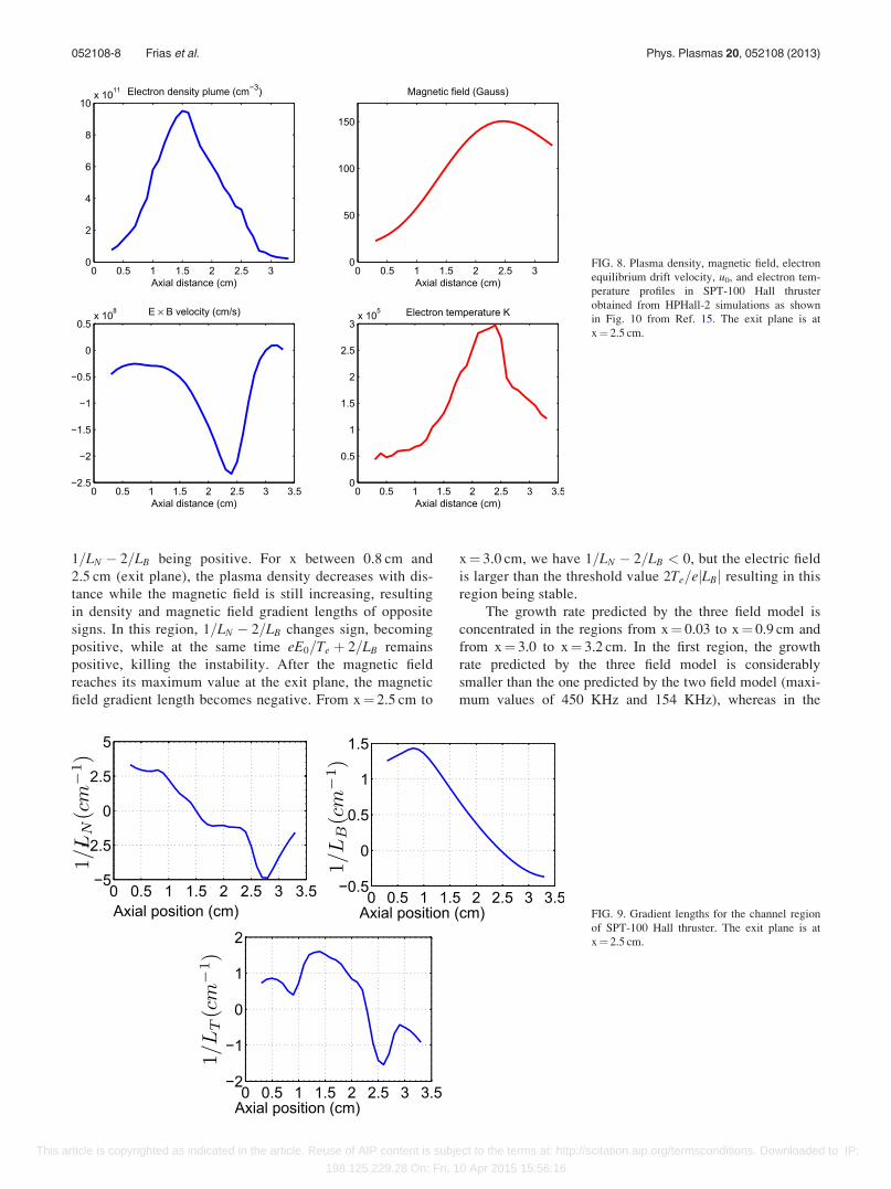
obtained plasma parameters profiles are shown in Fig. 8.
The magnetic field is positive and increasing with dis-
tance in the channel region, reaching a maximum at the chan-
nel exit and decreasing in the plume region, which results in a
positive magnetic field gradient length LB¼ð@ lnB=@xÞ�1 > 0
inside the channel and in a negative magnetic field gradient
length LB ¼ ð@ ln B=@xÞ�1 < 0 in the plume region. The
plasma density reaches its maximum value at a distance of
x¼ 1.5 cm from the anode, decreasing afterwards, resulting in
a positive density gradient length LN ¼ ð@ ln n=@xÞ�1 > 0
from x¼ 0.03 cm to x¼ 1.5 cm and in a negative density gra-
dient length LN ¼ ð@ ln n=@xÞ�1 < 0 after x¼ 1.5 cm. We
have, then, a region between x¼ 1.5 cm and x¼ 2.5 cm where
the density and magnetic field gradient lengths are of opposite
signs, with the density gradient length being negative and the
magnetic field gradient length being positive. This region is
FIG. 5. Magnetic field lines in the 12.3 cm Hall thruster for three magnetic
field configurations: B0, Bpos, and Bneg. All diagrams are drawn to scale.
Reprinted with permission from Phys. Plasmas 13, 057104 (2006). Copyright
2006 American Institute of Physics.14
052108-6 Frias et al. Phys. Plasmas 20, 052108 (2013)
This article is copyrighted as indicated in the article. Reuse of AIP content is subject to the terms at: http://scitation.aip.org/termsconditions. Downloaded to IP:
198.125.229.28 On: Fri, 10 Apr 2015 15:56:16

expected to be stable. The electron temperature reaches its
maximum value also at the exit plane, resulting in a positive
temperature gradient length LT ¼ ð@ ln Te=@xÞ�1 > 0 inside
the channel and in a negative temperature gradient length
LT ¼ ð@ ln Te=@xÞ�1 < 0 in the plume. Similarly to the mag-
netic field and electron temperature, the electric field reaches
its maximum value at the exit plane. The gradient lengths for
the plasma parameters from Fig. 8 are plotted in Fig. 9.
The growth rate and frequency (of the unstable modes
only) calculated by solving Eqs. (4) and (6) are shown in
Fig. 10.
For the profiles shown in Fig. 8, there is an unstable
region inside the channel from x¼ 0.03 cm to x¼ 0.8 cm,
which is close to the anode. This instability growth rate is
in the 100–450 KHz range, the growth rate being larger
when the temperature gradients are not considered. In this
region, 1=LN � 2=LB > 0 and since the electric field and the
magnetic field gradient length are both positive, the factor
eE0=Te þ 2=LB is positive, resulting in instability. The real
part of the frequency is determined by the sign of
1=LN � 2=LB. In the unstable region from x¼ 0.03 cm to
x¼ 0.8 cm, the frequency is negative due to the factor
FIG. 6. Three different profiles for mag-
netic field configuration and electron den-
sity and temperature measured at the
midpoint between the channel walls as
reported in Ref. 14.
FIG. 7. Growth rate and frequency of the
instabilities as a function of axial distance as
predicted by the two-field model for the pro-
files in Fig. 6.
052108-7 Frias et al. Phys. Plasmas 20, 052108 (2013)
This article is copyrighted as indicated in the article. Reuse of AIP content is subject to the terms at: http://scitation.aip.org/termsconditions. Downloaded to IP:
198.125.229.28 On: Fri, 10 Apr 2015 15:56:16
1=LN � 2=LB being positive. For x between 0.8 cm and
2.5 cm (exit plane), the plasma density decreases with dis-
tance while the magnetic field is still increasing, resulting
in density and magnetic field gradient lengths of opposite
signs. In this region, 1=LN � 2=LB changes sign, becoming
positive, while at the same time eE0=Te þ 2=LB remains
positive, killing the instability. After the magnetic field
reaches its maximum value at the exit plane, the magnetic
field gradient length becomes negative. From x¼ 2.5 cm to
x¼ 3.0 cm, we have 1=LN � 2=LB < 0, but the electric field
is larger than the threshold value 2Te=ejLBj resulting in this
region being stable.
The growth rate predicted by the three field model is
concentrated in the regions from x¼ 0.03 to x¼ 0.9 cm and
from x¼ 3.0 to x¼ 3.2 cm. In the first region, the growth
rate predicted by the three field model is considerably
smaller than the one predicted by the two field model (maxi-
mum values of 450 KHz and 154 KHz), whereas in the
FIG. 8. Plasma density, magnetic field, electron
equilibrium drift velocity, u0, and electron tem-
perature profiles in SPT-100 Hall thruster
obtained from HPHall-2 simulations as shown
in Fig. 10 from Ref. 15. The exit plane is at
x¼ 2.5 cm.
FIG. 9. Gradient lengths for the channel region
of SPT-100 Hall thruster. The exit plane is at
x¼ 2.5 cm.
052108-8 Frias et al. Phys. Plasmas 20, 052108 (2013)
This article is copyrighted as indicated in the article. Reuse of AIP content is subject to the terms at: http://scitation.aip.org/termsconditions. Downloaded to IP:
198.125.229.28 On: Fri, 10 Apr 2015 15:56:16

second region, the growth rate predicted by the two field
model is just slightly larger (maximum values of 64 KHz
and 43 KHz). The real part of the frequency predicted by the
three field model follows the same pattern as the one pre-
dicted by the two field model. In the unstable region in the
near anode region, from x¼ 0.03 cm to x¼ 0.8 cm, the fre-
quency is negative.
There is an interesting feature in the region between
x¼ 3.0 cm and x¼ 3.2 cm, where the unstable modes propa-
gate with positive frequency. The change of the direction of
the rotation is not related to temperature gradients (as was
the case in the HTX plume region, see Fig. 3(d)), which is
small here and therefore the two and three field model give
similar results. In this region, the electric field, within the ac-
curacy of the measurements, is smaller than the threshold
electric field, E < Ethr (situation unique among all the
regions investigated in this paper), and the instability crite-
rion is simply determined by the sign of the factor
1=LN � 2=LB; the mode is unstable for 1=LN � 2=LB < 0.
The sign of the real part of the frequency is only determined
by the sign of 1=LN � 2=LB, so that the instable modes prop-
agate with positive frequency (in the direction opposite to
E0 � B0). Generally, two field model predicts that the direc-
tion of propagation of unstable modes is directly linked to
the sign of the quantity ðE0 � EthrÞ � B0, thus negative (in
the direction of E0 � B0 flow) for E0 > Ethr, and positive
when E0 < Ethr. Some experiments with E0 � B0 plasmas do
show the presence of fluctuations with rotation in the direc-
tion opposite to E0 � B0 drift.21 Since our results are very
sensitive to the details of plasma parameters profiles, at this
time, we cannot confirm that profiles measurements and
postprocessing (e.g., profiles gradients) are accurate enough
to make conclusive statements regarding the robustness
of the rotation against the direction of E0 � B0 in the
experimental conditions discussed in this paper. Indeed, a
small perturbation of the plasma plume (induced by the
probe, for example) could alter these measurements. More
accurate measurements are needed to corroborate the predic-
tions of our model.
D. CAMILA thruster simulations
The CAMILA thruster, developed at the Technion’s
Asher Space Research Institute, is an effort to adapt Hall
thruster technology to low power regimes.16 In this device,
two concentric cylindrical electrodes are used as an anode.
The thruster channel consists of the anode cavity and the
dielectric walls of the thruster. The magnetic circuit pro-
duces a longitudinal magnetic field inside the anode cavity,
thus reducing the electron mobility in the radial direction. A
radial electric field is created in the direction towards the
center of the channel. The radial electric field will increase
electron energy in such a way that the gas inside the cavity
will be ionized. One advantage of this configuration is that
the whole length of the channel can be used for ionization.
Two configurations are currently under development, simpli-
fied CAMILA, without anode coils and full CAMILA, with
anode coils. In the following, we will refer to the simplified
version of the thruster. A more detailed description of the
CAMILA concept can be found in Ref. 16 and references
therein.
The plasma parameter profiles for the CAMILA thruster
are shown in Fig. 11 The magnetic field is positive and
increasing with distance in the channel region, reaching its
maximum value at the channel exit, located at x¼ 0, which
results in a positive magnetic field gradient length LB ¼ð@ ln B=@xÞ�1 > 0 inside the channel, except for the region
from x¼�3.0 to� 2.9 cm. The plasma density reaches its
FIG. 10. Growth rate and frequency of the
instabilities in a SPT-100 thruster15 as a
function of axial distance to the anode as
predicted by the two-field model ((a) and
(b)) and the three-field model ((c) and (d)).
The exit plane is at x¼ 2.5 cm.
052108-9 Frias et al. Phys. Plasmas 20, 052108 (2013)
This article is copyrighted as indicated in the article. Reuse of AIP content is subject to the terms at: http://scitation.aip.org/termsconditions. Downloaded to IP:
198.125.229.28 On: Fri, 10 Apr 2015 15:56:16

maximum value at a distance of x¼�0.8 cm from the exit
plane, decreasing afterwards, resulting in a positive density
gradient length LN ¼ ð@ ln n=@xÞ�1 > 0 from x¼�3.0 cm to
x¼�0.8 cm and in a negative density gradient length
LN ¼ ð@ ln n=@xÞ�1 < 0 from x¼�0.8 cm up to the exit
plane. We have, then, a region between x¼�3.0 and �2.9
and x¼�0.8 cm to x¼ 0 where the density and magnetic
field gradient lengths are of opposite signs, with the density
gradient length being negative and the magnetic field gradi-
ent length being positive. The instability is not present in this
region. The electron temperature reaches its maximum value
close to the exit plane, at x¼�0.4 cm, resulting in a positive
temperature gradient length LT ¼ ð@ ln Te=@xÞ�1 > 0 for
most of the region under consideration. Similarly to the mag-
netic field and electron temperature, the electric field reaches
its maximum value at the exit plane. The gradient lengths for
the plasma parameters from Fig. 11 are plotted in Fig. 12.
One peculiarity of the CAMILA magnetic field is the
additional presence of an axial component. This way, the
magnetic field B0 in dispersion relations, Eqs. (4) and (6),
refers to the magnitude of the field. The growth rate and fre-
quencies of the unstable modes calculated by solving Eqs.
(4) and (6) are shown in Fig. 13.
For the profiles shown in Fig. 11, there are two unstable
regions close to the anode. The first of these regions corre-
sponds to the interval from x¼�2.8 cm to x¼�2.5 cm,
where the maximum value for the growth rate is 280 KHz at
x¼�2.5 cm. The second unstable region corresponds to the
interval from x¼�2.0 cm to x¼�1.9 cm, where the peak of
the growth rate is 367 KHz at a position x¼�2.0 cm. These
two unstable regions have 1=LN � 2=LB > 0 and since the
electric field and the magnetic field gradient length are both
positive, the factor eE0=Te þ 2=LB is positive, resulting in
the appearance of the instability. For x between �1.9 cm and
the exit plane, the plasma density decreases with distance
while the magnetic field is still increasing, resulting in den-
sity and magnetic field gradient lengths of opposite signs. In
this region, the factor 1=LN � 2=LB becomes negative while
eE0=Te þ 2=LB remains positive, resulting in the disappear-
ance of the instability. In the unstable regions, since
1=LN � 2=LB > 0, the real part of the frequency is negative.
Using the three field model, the instability exists from
x¼�2.9 cm to x¼�2.4 cm and has a maximum value of
508 KHz at x¼�2.4 cm and from x¼�2.1 cm and
�1.7 cm, with a maximum value of 210 KHz at x¼�1.7 cm.
Similar to the previous examples, the growth rate of the
FIG. 12. Gradient lengths for the channel region of CAMILA Hall thruster.
The exit plane is at x¼ 0.
FIG. 11. Plasma density, magnetic field, elec-
tron equilibrium drift velocity, u0, and electron
temperature profiles in CAMILA Hall thruster
from Ref. 16. The exit plane is at x¼ 0.
052108-10 Frias et al. Phys. Plasmas 20, 052108 (2013)
This article is copyrighted as indicated in the article. Reuse of AIP content is subject to the terms at: http://scitation.aip.org/termsconditions. Downloaded to IP:
198.125.229.28 On: Fri, 10 Apr 2015 15:56:16

instability is smaller when the temperature gradients are con-
sidered, but in this case, the unstable region is continuous
and somewhat broader than that of the two field model. For
the three field model, the real part of the frequency is
negative.
IV. SUMMARY
The dispersion relations for the two and three field mod-
els derived in Part I were used to study the instabilities in four
different configuration using the experimental and simulations
results. It is interesting that for all configurations, the instabil-
ities are in the near anode and in the plume regions, where the
gradient lengths are of the same sign, positive for the near
anode region and negative in the plume region. In addition
to this, the instability exists in regions between the change
of sign of either one of the factors 1=LN � 2=LB and
eE0=Te þ 2=LB, with sharp peaks in the regions where there
is a change of the sign in the factor 1=LN � 2=LB. This condi-
tion follows from Eq. (5), where both factors 1=LN � 2=LB
and eE0=Te þ 2=LB are required to be of the same sign. One
important result is that the Morozov condition predicts insta-
bility in a wider spatial region than the one predicted by our
model. Also in the plume region, where the magnetic field
gradient length is negative, when the factor 1=LN � 2=LB is
positive, the instability requires that the electric field be larger
than a certain threshold value given by E0;thr ¼ 2Te=ejLBj. If
the contrary happens, that is, 1=LN � 2=LB < 0, like in the
unstable region in the plume of the SPT-100 thruster, the
instability occurs if the electric field is smaller than the thresh-
old E0;thr ¼ 2Te=ejLBj. In the near anode region, since the
magnetic field gradient length and the factor eE0=Te þ 2=LB
(for E0 > 0) are positive, the instability requires that
1=LN � 2=LB > 0.
The highest growth rates are observed in the plume
region for the HTX thruster and in the near anode region for
the SPT-100 and CAMILA thrusters. In all thrusters, the addi-
tion of temperature gradients reduces the peak value of the
instability, with the reduction being in as much as 40% for the
plume region of the HTX thruster, 60% for the near anode
region of the SPT-100 thruster, and 50% for CAMILA. In the
near anode region of the HTX thruster, with the magnetic field
near the anode, the magnetic field gradient dominates over the
density and temperature gradients and the predictions of the
two and three field model do not differ considerably.
The conditions for the instability are different depending
on the sign of plasma density and magnetic field gradients.
Particular conditions existing in different thrusters are sum-
marized in Table I. In the near anode region, where the gra-
dients of the magnetic field and density are both positive, the
instability is driven by large density gradient, while the mag-
netic field gradient is stabilizing. In the plume region, where
the gradients of the magnetic field and density are both nega-
tive, either magnetic field gradient or the density gradient can
be destabilizing, depending on the amplitude of the electric
field.
The azimuthal phase velocity of the instabilities, defined
as xr=ky, has a maximum value of around �15 000 m/s for
FIG. 13. Growth rate and frequency of
the instabilities in the CAMILA thruster16
as a function of axial distance to the anode
as predicted by the two-field model ((a)
and (b)) and the three-field model ((c) and
(d)). The exit plane is at x¼ 0.
TABLE I. Conditions for instability in different regions of Hall thrusters.
Condition I: 1LN� 2
LB> 0; E > Ethr . Condition II: 1
LN� 2
LB< 0; E < Ethr .
Thruster Near anode (LB, LN > 0) Plume (LB, LN < 0)
HTX (Ref. 13) No data I
HTX (Ref. 14) I No data
SPT-100 (Ref. 15) I II
CAMILA (Ref. 16) I No data
052108-11 Frias et al. Phys. Plasmas 20, 052108 (2013)
This article is copyrighted as indicated in the article. Reuse of AIP content is subject to the terms at: http://scitation.aip.org/termsconditions. Downloaded to IP:
198.125.229.28 On: Fri, 10 Apr 2015 15:56:16

the plume region of HTX, �1500 m/s for the anode region of
HTX with the Bpos configuration and 600 m/s with the Bneg
configuration, �40 m/s for both SPT-100 and CAMILA.
These values are close to the azimuthal phase velocities
observed for the rotating spoke instability.4
It is interesting to note that despite difference in designs,
all configurations studied here show common feature of the
instabilities concentrated in the region near the anode and in
the plume region (as far as available data show) and the ab-
sence of the instabilities in the acceleration region of the
thrusters, close to the maximum values of the electric and
magnetic fields.
The primary driving source of the long wavelength
instabilities studied in this paper is the equilibrium electron
current. The instability can be triggered by collisions, as con-
sidered in Ref. 22 or by gradients of plasma density, temper-
ature, and/or magnetic field, which are considered in this
paper. Various approximations lead to several different mod-
els discussed in the Introduction. Our result for two-fluid
model differs in numerical factors from the model by
Kapulkin in Ref. 8 because of their incomplete account of
compressibility, for more details see Part I. In Fig. 14, the
growth rate of the instabilities derived by Kapulkin (Eq. (19)
in Ref. 8) is compared with the growth rate predicted by our
two-field-model. The growth rate for the anti-drift instability
from Eq. (9) is also shown in the same figure. The growth
rate predicted by the Kapulkin model is larger than the one
predicted by the two-field model in the near anode region,
but it is smaller in the plume region. The growth rate is sig-
nificantly smaller without the gradients of the magnetic field
as, as predicted by Eq. (9).
The real part of the frequency for various discharges is
shown in Figs. 3, 10, and 13. The mode phase velocity is typ-
ically in the same direction as E�B drift (which is negative
in our notations) but it is not related to the E�B drift
directly. Rather, it is determined by the inverse of the x� �xD frequency (see Eq. (4)). As a result, the real part of the
frequency scales inversely with the ion mass, xr � m�1i ; the
growth rate has inverse dependence on the square root of the
ion mass, c � ðmiÞ�1=2. As follows from our calculations,
the phase velocity of this mode is roughly one order of mag-
nitude lower than E�B velocity (for typical parameters con-
sidered here), that is consistent with the spoke phase
velocity.4 The inverse mass dependence seems also generally
consistent with spoke velocity in other experiments,23–25
which may suggest that drift gradient modes are responsible
for spoke phenomena and no critical ionization phenomena
may be involved. As was noted in the Introduction, partial
magnetization of ion motion results in the additional term
kyvhi to the real part of the frequency. This is the regime of
the so called modified Simon-Hoh instability, see Ref. 12
and references therein. Calculation of the average ion drift
velocity vhi, in general, requires knowledge of the global
electric field profile and is not attempted here. An estimate
based on Eq. (10) predicts12 that kyvhi contribution may be
comparable or exceed the real part of the frequency for the
anti-drift mode in Eq. (4), thus changing the scaling for the
real part of the mode frequency from 1=mi for the anti-drift
mode to 1=ffiffiffiffiffimip
for the modified Simon-Hoh mode. It is
worth noting that though the near marginal stability bound-
ary effects of magnetic field gradient result in higher values
of the real part of the frequency, the role of the ion azimuthal
drift may be less pronounced.
As was discussed in the Introduction, Esipchuk and
Tilinin have considered physically similar model of the gra-
dient drift instability but used the relations (12) and (13) to
express the density gradient via the electric field resulting in
Eq. (16). The solution of Eq. (16) is compared with the solu-
tion to the two field model dispersion relation (Eq. (4)), for
the profiles in Figs. 1, 8, and 11 in Fig. 15. As one can see
FIG. 14. Growth rate of the instabilities for
the (a) HTX thruster, (b) SPT-100, and (c)
CAMILA, as predicted by the two-field
model, Eq. (19) from Ref. 8 and antidrift
instability.6,12
052108-12 Frias et al. Phys. Plasmas 20, 052108 (2013)
This article is copyrighted as indicated in the article. Reuse of AIP content is subject to the terms at: http://scitation.aip.org/termsconditions. Downloaded to IP:
198.125.229.28 On: Fri, 10 Apr 2015 15:56:16

from Fig. 15, there is substantial difference between these
models: essentially the model of Eq. (16) does not predict
the instability in most of the regions. If we would have used
the model with the actual density profile, as in Eq. (17), the
predictions will be similar to the Kapulkin model, with only
quantitative differences with our two-fluid model as shown
in Fig. 14.
As was noted above, the derivation of the dispersion
relation (16) is based on the assumption that n0v0i remains
constant. The data confirm that the assumption that
nðxÞv0i¼ constant is not met, especially near the channel exit,
as can be seen from Fig. 16. Therefore, the model of Ref. 7,
which is typically used in the form given by Eq. (16), gives
significantly different results, due to discrepancy of the ion
density profile from the nðxÞv0i¼ constant predictions. The
deviation of nðxÞv0i from constant may be related to several
factors such as radial divergence of the ion flow and ionization
processes. In addition to the modification of the equilibrium
density profile, ionization process may be lead to specific ioni-
zation instabilities,26 which are not considered here.
FIG. 15. Growth rate of the instability as
predicted by the two field model and by
Eq. (16) for (a) HTX thruster, (b) SPT-
100, and (c) CAMILA.
FIG. 16. Product n0v0i for the (a) HTX
thruster, (b) SPT-100, and (c) CAMILA.
052108-13 Frias et al. Phys. Plasmas 20, 052108 (2013)
This article is copyrighted as indicated in the article. Reuse of AIP content is subject to the terms at: http://scitation.aip.org/termsconditions. Downloaded to IP:
198.125.229.28 On: Fri, 10 Apr 2015 15:56:16
Ducrocq et al.27 also studied the high frequency, short
wavelength instability excited by the resonances between the
term kyu0 and harmonics of the electron cyclotron frequency
nXe. Such instabilities cannot be described by our fluid
theory. According to Ref. 27, for the typical Hall thruster pa-
rameters, this instability is robust with respect to the gra-
dients of plasma density and exists mainly in the exit plane
of the Hall thruster, where the E�B drift velocity is maxi-
mal. This instability occurs as a result of coupling of the
electron cyclotron mode and the ion sound and was studied
in detail in Refs. 28–30. These modes are typically highly
aperiodic (with growth rates exceeding the real part of the
frequency by orders of magnitude), which is consistent with
some features observed experimentally.31 Nonlinear theory
and simulations28–30 predict though that due to large wave-
vector, these modes saturate at low amplitudes and do not
lead to significant anomalous transport.
Our main emphasis was on the analysis of azimuthal
modes (with finite ky). Note that according to Eq. (3), the
drift gradient mode may also acquire the axial group velocity
due the ion motion in axial direction. Such transit ion modes
were studied in Refs. 32 and 33, though the destabilization
mechanisms considered in Refs. 32 and 33 were due to colli-
sions and ionization. Our analysis shows that drift gradient
effects may also lead to the excitation of the mode with ion
group velocity in the axial direction.
The conditions for the linear excitation, general mode
characteristics such as frequency and growth rate, the mode
localizations of the gradient drift modes studied in this paper
are generally consistent with some experimental features,
and thus may be responsible for anomalous electron mobility
and nonlinear structures. The investigations of the latter
require nonlinear theory and nonlinear simulations which are
left for other publication.
ACKNOWLEDGMENTS
The authors thank Dr. Nathaniel J. Fisch for helpful dis-
cussions, Dr. Richard Hofer for allowing the use of the data
from the HPHall-2 simulations and Dr. Igal Kronhaus and Dr.
Alexander Kapulkin for providing the data for the CAMILA
Hall thruster. This work was sponsored by the Natural
Sciences and Engineering Research Council of Canada and
partially supported by the Air Force Office of Scientific
Research and the US Department of Energy.
1M. Keidar and I. Beilis, IEEE Trans. Plasma Sci. 34, 804 (2006).2G. J. M. Hagelaar, J. Bareilles, L. Garrigues, and J. P. Boeuf, J. Appl.
Phys. 93, 67 (2003).3J. C. Adam, J. P. Boeuf, N. Dubuit, M. Dudeck, L. Garrigues, D.
Gresillon, A. Heron, G. J. M. Hagelaar, V. Kulaev, N. Lemoine, S.
Mazouffre, J. P. Luna, V. Pisarev, and S. Tsikata, Plasma Phys. Controlled
Fusion 50, 124041 (2008).4C. L. Ellison, Y. Raitses, and N. J. Fisch, Phys. Plasmas 19, 013503 (2012).5M. E. Griswold, C. L. Ellison, Y. Raitses, and N. J. Fisch, Phys. Plasmas
19, 053506 (2012).6W. Frias, A. I. Smolyakov, I. D. Kaganovich, and Y. Raitses, Phys.
Plasmas 19, 072112 (2012).7Y. V. Esipchuk and G. N. Tilinin, Sov. Phys. Tech. Phys. 21, 417 (1976).8A. Kapulkin and M. M. Guelman, IEEE Trans. Plasma Sci. 36, 2082
(2008).9A. Simon, Phys. Fluids 6, 382 (1963).
10F. C. Hoh, Phys. Fluids 6, 1184 (1963).11A. M. Fridman, Sov. Phys. Dokl. 9, 072112 (1964).12Y. Sakawa, C. Joshi, P. K. Kaw, F. F. Chen, and V. K. Jain, Phys. Fluids B
5, 1681 (1993).13Y. Raitses, D. Staack, M. Keidar, and N. Fisch, Phys. Plasmas 12, 057104
(2005).14L. Dorf, Y. Raitses, and N. J. Fisch, Phys. Plasmas 13, 057104 (2006).15R. Hofer, I. Mikellides, I. Katz, and D. Goebel, in 43rd AIAA/ASME/SAE/
ASEE Joint Propulsion Conference & Exhibit, AIAA 2007-5267, 2007.16I. Kronhaus, A. Kapulkin, V. Balabanov, M. Rubanovich, M. Guelman,
and B. Natan, J. Phys. D: Appl. Phys. 45, 175203 (2012).17A. Hirose and I. Alexeff, Nucl. Fusion 12, 315 (1972).18A. I. Morozov, Y. V. Esipchuk, A. Kapulkin, V. Nevrovskii, and V. A.
Smirnov, Sov. Phys. Tech. Phys. 17, 482 (1972).19F. Parra, E. Ahedo, J. Fife, and M. Martinez-Sanchez, J. Appl. Phys. 100,
023304 (2006).20J. Fife, Ph.D. dissertation, Aeronautics and Astronautics, Massachusetts
Institute of Technology, 1998.21T. Ito and M. A. Cappelli, IEEE Trans. Plasma Sci. 36, 1228 (2008).22A. A. Litvak and N. J. Fisch, Phys. Plasmas 8, 648 (2001).23N. Brenning and D. Lundin, Phys. Plasmas 19, 093505 (2012).24A. Lazurenko, L. Albarede, and A. Bouchoule, Phys. Plasmas 13, 083503
(2006).25A. Lazurenko, G. Coduti, S. Mazouffre, and G. Bonhomme, Phys. Plasmas
15, 034502 (2008).26D. Escobar and E. Ahedo, in International Electric Propulsion
Conference, Wiesbaden, Germany (2011), Paper No. IEPC-2011-196.27A. Ducrocq, J. C. Adam, A. Heron, and G. Laval, Phys. Plasmas 13,
102111 (2006).28C. Lashmore-Davies and T. Martin, Nucl. Fusion 13, 193 (1973).29M. Lampe, W. M. Manheimer, J. B. McBride, J. H. Orens, R. Shanny, and
R. N. Sudan, Phys. Rev. Lett. 26, 1221 (1971); M. Lampe, W. M.
Manheimer, J. B. McBride, J. H. Orens, K. Papadopoulos, R. Shanny, and
R. N. Sudan, Phys. Fluids 15, 662 (1972).30H. V. Wong, Phys. Fluids 13, 757 (1970).31S. Tsikata, N. Lemoine, V. Pisarev, and D. M. Gresillon, Phys. Plasmas
16, 033506 (2009).32S. Barral, K. Makowski, Z. Peradzynski, and M. Dudeck, Phys. Plasmas
12, 073504 (2005).33E. Fernandez, M. K. Scharfe, C. A. Thomas, N. Gascon, and M. A.
Cappelli, Phys. Plasmas 15, 012102 (2008).
052108-14 Frias et al. Phys. Plasmas 20, 052108 (2013)
This article is copyrighted as indicated in the article. Reuse of AIP content is subject to the terms at: http://scitation.aip.org/termsconditions. Downloaded to IP:
198.125.229.28 On: Fri, 10 Apr 2015 15:56:16