Primordial Perturbations from a Self-interacting Curvaton

HELSINKI INSTITUTE OF PHYSICS INTERNAL REPORT SERIES

HIP-2010-04

Primordial Perturbationsfrom a Self-interacting Curvaton

Olli Taanila

Helsinki Institute of PhysicsUniversity of Helsinki

Finland

ACADEMIC DISSERTATION

To be presented, with the permission of the Faculty of Scienceof the University of Helsinki, for public criticism

in the auditorium CK112 of Exactum, Gustaf Hallstromin katu 2 B,on the 15th of December 2010 at 10 o’clock.

Helsinki 2010

ISBN 978-952-10-5324-5 (paperback)ISSN 1455-0563

ISBN 978-952-10-5323-8 (pdf)http://ethesis.helsinki.fi/

YliopistopainoHelsinki 2010

Acknowledgements

This thesis is based on research carried out in Helsinki Institute of Physics and the De-partment of Physics of University of Helsinki. The work has been partially funded bya grant from the Magnus Ehrnrooth Foundation and supported by the EU 6th Frame-work Marie Curie Research and Training network “UniverseNet”.

I have the privilege to thank my supervisor Kari Enqvist. For the past few yearsthat I have been working with him, we have shared many interesting and entertainingdiscussions. He has not only been an excellent supervisor, but I also consider him tobe a relaxed yet enthusiastic colleague. Moreover, we apparently share a similar viewon how to serve green asparagus. Another significant mentor of mine has been KeijoKajantie, who was the person originally responsible for hiring me to the department.As a friend of ours once said, Keijo has a very admirable attitude towards both scienceand life.

Gerasimos Rigopoulos, Anders Tranberg and Patta Yogendran have tutored me inmy early steps of research, and for that I am very grateful. They have taught me alot about physics, especially the more practical side of it. I also wish to thank AndersTranberg for reading the manuscript and offering many insightful comments on it.Similarly I wish to thank the referees of the thesis, Arttu Rajantie and Shinta Kasuya,for valuable comments.

I also wish to thank my other collaborators, namely Anupam Mazumdar, SamiNurmi, Philip Stephens and Tomo Takahashi. They have all made our collaborationfun and eased, yet insightful and fruitful. It has been an enjoyable experience to workon these papers with all of them.

During my undergraduate and graduate studies in Helsinki I have been priviledgedto attend many excellent courses. Of the exceptional teachers in the department onemust mention Claus Montonen, Hannu Kurki-Suonio and especially Juha Honkonen.There have also been an enormous number of officemates and co-students with whomI have had the pleasure not only to study, but to also babble about all things betweenend of inflation and our exercises, and I want to thank them all. Especially I wantto acknowledge the trio of noisiest theoretical physics graduate students Helsinki hasever known, with whom I have enjoyed countless hours of badminton.

Last but not least I wish to thank my parents and my significant other for supportand not-too-loud criticism of my choice of career.

Helsinki, November 2010

Olli Taanila

iii

Taanila, Olli: Primordial perturbations from a self-interacting curvaton,University of Helsinki, 2010, 85 pages,Helsinki Institute of Physics Internal Report Series, HIP-2010-04,ISSN 1455-0563ISBN 978-952-10-5324-5.

Keywords: cosmology, curvaton, primordial perturbations, self-interactions.

Abstract

Inflation is a period of accelerated expansion in the very early universe, which has theappealing aspect that it can create primordial perturbations via quantum fluctuations.These primordial perturbations have been observed in the cosmic microwave back-ground, and these perturbations also function as the seeds of all large-scale structurein the universe. Curvaton models are simple modifications of the standard inflationaryparadigm, where inflation is driven by the energy density of the inflaton, but anotherfield, the curvaton, is responsible for producing the primordial perturbations.

Since the curvaton must decay, it must have some interactions. Additionally real-istic curvaton models typically have some self-interactions. In this work we considerself-interacting curvaton models, where the self-interaction is a monomial in the po-tential, suppressed by the Planck scale, and thus the self-interaction is very weak.Nevertheless, since the self-interaction makes the equations of motion non-linear, itcan modify the behaviour of the model very drastically. The most intriguing aspect ofthis behaviour is that the final properties of the perturbations become highly depen-dent on the initial values.

Departures of Gaussian distribution are important observables of the primordialperturbations. Due to the non-linearity of the self-interacting curvaton model andits sensitivity to initial conditions, it can produce significant non-Gaussianity of theprimordial perturbations. In this work we investigate the non-Gaussianity producedby the self-interacting curvaton, and demonstrate that the non-Gaussianity parametersdo not obey the analytically derived approximate relations often cited in the literature.

Furthermore we also consider a self-interacting curvaton with a mass in the TeV-scale. Motivated by realistic particle physics models such as the Minimally Super-symmetric Standard Model, we demonstrate that a curvaton model within the massrange can be responsible for the observed perturbations if it can decay late enough.

iv

List of Publications

The content of this thesis is based on the following research articles [1–3]:

I The Subdominant Curvaton,K. Enqvist, S. Nurmi, G. Rigopoulos, O. Taanila and T. Takahashi,JCAP 0911 (2009) 003.

II Non-Gaussian Fingerprints of Self-Interacting Curvaton,K. Enqvist, S. Nurmi, O. Taanila and T. Takahashi,JCAP 1004 (2010) 009.

III The TeV-mass Curvaton,K. Enqvist, A. Mazumdar and O. Taanila,JCAP 1009 (2010) 030.

In all of the papers the authors are listed alphabetically according to the particlephysics convention.

The Author’s Contribution to the Joint Publications

I The inital idea to study subdominant curvaton models was T. Takahashi’s. Thepresent author performed the initial analytical calculations and wrote a com-puter program to solve the model numerically. Excluding the analytical treatisewhich was written by S. Nurmi, and the section concerning the Fokker-Planckequation which was written by G. Rigopoulos, the present author wrote the firstdraft of the paper, which was then polished jointly by all authors.

II The program developed for I was further improved by the present author by im-plementing a method to calculate the non-Gaussianity parameters. The presentauthor calculated all the results and produced all of the plots, as well as wrotethe first draft of the paper.

III The pre-existing code was used by the present author to calculate the results.Also the analytical calculations were mostly done by the present author. A. Mazum-dar wrote the parts of the draft discussing MSSM and Q-balls and K. Enqvistthe introduction and discussion. The rest was drafted by the present author andthen polished jointly with K. Enqvist.

v

Units and Conventions

In this work we use natural units, i.e., we set three constants of nature to unity,

„ D c D kB D 1 :

For most of this work, we use units of electronvolts, eV, or multiples thereof, such asgigaelectronvolts, GeV, as the measure of energy and consequently all dimensionfulquantities.

We denote the reduced Planck mass by

MPl D

r„c

8�G:

In the three papers, on which this thesis is based, we set the reduced Planck massoften to unity, i.e., express all dimensionful variables as powers ofMPl. Nevertheless,we refrain from setting it to unity in the main text.

For Fourier transforms we use the normalization convention where the factors of2� are included in the inverse transformation,

f .x/ D

Zd3k.2�/3

eik�xfk ; fk D

Zd3x e�ik�xf .x/ :

As most of this work is concerned with investigating the evolution of certainquantities from the end of inflation to some much later point in time, we adopt theshort-hand notation where the subscript � denotes a quantity evaluated at the end ofinflation, e.g. H� is the Hubble constant at the end of inflation.

In the literature there has been a mixture of notations concerning the factor r . Itdenotes the energy density of the curvaton �� compared with the total energy den-sity of the universe. For this work we adopt a very useful, though a bit inconsistentnotation where r denotes the energy fraction in the curvaton field,

r ��

†i�i;

while r� describes the energy density of the curvaton compared to that of the back-ground at the end of inflation,

r� ��

�r

ˇend of inflation

;

vi

and rdec, in discrepancy with the preceding definition of r , measures the quantity oftenreferred to as r in the literature,

rdec �3��

3�� C 4�r

ˇcurvaton decay

;

also called the efficiency factor. Note that these definitions somewhat differ from thenotation used in the attached publications.

vii

Contents

Acknowledgements . . . . . . . . . . . . . . . . . . . . . . . . . . . . . . iiiAbstract . . . . . . . . . . . . . . . . . . . . . . . . . . . . . . . . . . . . ivList of Publications . . . . . . . . . . . . . . . . . . . . . . . . . . . . . . vUnits and Conventions . . . . . . . . . . . . . . . . . . . . . . . . . . . . vi

1 Introduction 11.1 Friedmann-Robertson-Walker Cosmology . . . . . . . . . . . . . . . 11.2 The Hot Big Bang and the CMB . . . . . . . . . . . . . . . . . . . . 31.3 Inflation . . . . . . . . . . . . . . . . . . . . . . . . . . . . . . . . . 41.4 Primordial Perturbations . . . . . . . . . . . . . . . . . . . . . . . . 6

2 Cosmological Perturbation Theory 92.1 The Perturbed Metric . . . . . . . . . . . . . . . . . . . . . . . . . . 92.2 Gauge Invariant Perturbations . . . . . . . . . . . . . . . . . . . . . 112.3 Evolution of the Perturbations . . . . . . . . . . . . . . . . . . . . . 122.4 The Power Spectrum . . . . . . . . . . . . . . . . . . . . . . . . . . 132.5 �N -formalism . . . . . . . . . . . . . . . . . . . . . . . . . . . . . 14

3 Generating Perturbations 173.1 Quantizing a Scalar Field in de Sitter Space . . . . . . . . . . . . . . 173.2 Scaling Solutions for Oscillating Fields . . . . . . . . . . . . . . . . 213.3 Slow-roll Inflation . . . . . . . . . . . . . . . . . . . . . . . . . . . . 233.4 The Curvaton Scenario . . . . . . . . . . . . . . . . . . . . . . . . . 26

4 Non-Gaussianity of the Primordial Perturbations 294.1 Non-Gaussianity in the �N -formalism . . . . . . . . . . . . . . . . . 304.2 Non-Gaussianity in Single Field Slow-roll Inflation . . . . . . . . . . 314.3 Non-Gaussianity Parameters in the Curvaton Scenario . . . . . . . . . 32

5 Importance of Self-interactions 355.1 The Lower Limit for the Decay Constant � . . . . . . . . . . . . . . 355.2 Bounds in the Parameter Space . . . . . . . . . . . . . . . . . . . . . 37

5.2.1 Curvature Bound . . . . . . . . . . . . . . . . . . . . . . . . 37

viii

ix

5.2.2 Non-Gaussianity Bound . . . . . . . . . . . . . . . . . . . . 375.2.3 The Isocurvature Bound . . . . . . . . . . . . . . . . . . . . 38

5.3 Importance of the Self-interactions . . . . . . . . . . . . . . . . . . . 39

6 Dynamics of Self-interactions 456.1 Analytical Estimates for the Self-interacting Case . . . . . . . . . . . 456.2 Numerical Analysis . . . . . . . . . . . . . . . . . . . . . . . . . . . 47

6.2.1 Non-Gaussianity . . . . . . . . . . . . . . . . . . . . . . . . 496.3 Evolution of r . . . . . . . . . . . . . . . . . . . . . . . . . . . . . . 496.4 Evolution of �N . . . . . . . . . . . . . . . . . . . . . . . . . . . . 516.5 Oscillations in the Parameter Space . . . . . . . . . . . . . . . . . . 526.6 Comparison with the Analytical Estimates for fNL and gNL . . . . . . 55

7 Results in the Parameter Space 577.1 Allowed Regions of the Parameter Space . . . . . . . . . . . . . . . . 577.2 Effect of Constraints in Parameter Space . . . . . . . . . . . . . . . . 597.3 Scan of the Parameter Space . . . . . . . . . . . . . . . . . . . . . . 607.4 The TeV-mass Curvaton . . . . . . . . . . . . . . . . . . . . . . . . . 61

7.4.1 Additional Mechanisms to Facilitate Small Values of � . . . . 62

8 Conclusions 65

Chapter 1

Introduction

Modern cosmology offers a detailed description of the evolution of the universe fromits very first picoseconds until the present day. It predicts accurately the amount of dif-ferent elements present in the universe [4–6], and it explains the evolution of structureon large scales as well as the formation of non-linear structures on smaller scales. Thisstandard description of the universe is often calledƒCDM, comparable to the StandardModel of particle physics. ƒCDM however has several ingredients which invite a morerigorous understanding: What is the nature of dark matter and dark energy, what isthe source of the baryon asymmetry in the universe, and what is the mechanism forinflation in the very early universe?

The topic of this thesis is the generation of primordial perturbations in curvatonmodels. The primordial perturbations are usually thought to originate during infla-tion, and they function as the primordial seeds for all structure in the universe: stars,galaxies, clusters etc. The curvaton models are a modification of the run-of-the-millinflationary models.

1.1 Friedmann-Robertson-Walker Cosmology

The universe is described exceptionally well by a spatially homogeneous and isotropicuniverse. The most generic metric realizing these symmetries is the Friedmann-Robertson-Walker cosmology [7–11], described by the metric

ds2 D �dt2 C a2.t/

�dr2

1 �Kr2C r2d�2 C r2 sin2� d�2

�: (1.1)

Here K determines the geometry of slices of constant time: The case K D �1 corre-sponds to a hyperbolic universe, K D 1 corresponds to a closed universe, and K D 0

to a flat universe. Observationally we know thatK is extremely close to zero [12, 13],and thus henceforth we set it to zero.

2 Introduction

The scale factor a.t/ encodes information about the evolution of distances in theuniverse, and its evolution determines the expansion of the universe. Due to the afore-mentioned symmetries of the FRW-model, the scale factor can have evolution only intime. The time evolution of a.t/ is determined by the energy content of the universe.The equation of motion for a.t/ is to be derived from equations of motion for thewhole metric, which in general relativity are given by the Einstein equations

R�� 1

2Rg�� D 8�GT�� : (1.2)

Here the metric g�� is the fundamental dynamical quantity, whereas R and R�� arerespectively the Ricci scalar and the Ricci tensor, which encode information of thecurvature of the metric. They consist of derivatives of g�� , and their computation isdiscussed in more detail in section 2.3.

The information about the energy content of the universe is given by the energymomentum tensor. In the rest frame of an ideal fluid the energy-momentum tensor canbe written as T �� D diag.��; p; p; p/, and thus the continuity equation r�T

�� D 0,analogous to the energy and momentum conservation in flat space, can be written as

P�C 3H.�C p/ D 0 ;

where � and p are the energy density and pressure, and H is the Hubble parameter,H � Pa=a, which measures the expansion speed of the universe. For a fluid with aconstant equation of state parameter w � p=�, a scaling law can thus be written (seealso section 3.2 for the case of homogeneous oscillating fields) for the energy density:

�.t/ / a�3.1Cw/.t/ :

The Einstein equation (1.2) has two free indices, and is thus actually a set of4�4�6 D 10 equations. Nevertheless, due to the symmeries of the FRW metric onlyvery few of the equations are independent. Writing the 0 � 0 and i � i componentsseparately, and substracting them from each other, one ends up with the Friedmannequations,

H 2D

�Pa

a

�2D8�G

3� (1.3)

Ra

aD �

4�G

3.�C 3p/ : (1.4)

Here the dot denotes the usual temporal derivative,

P �d

dt:

The Friedmann equations encode the information of how the energy content ofthe universe affects the expansion of the universe. The scale factor a.t/ in the metricof the equation (1.1) is thus to be solved for in the Friedmann equations.

1.2 The Hot Big Bang and the CMB 3

The coordinates in equation (1.1) correspond to physical time and comoving spa-tial coordinates, meaning that while the time coordinate t is the actual time measuredby a comoving observer, the fixed coordinate distances correspond to increasing phys-ical distances due to the evolution of a.t/. Often it is more convenient to use confor-mal time �, defined by the infinitesimal expression

d� Ddta.t/

: (1.5)

Intuitively this means that the new time coordinate scales according to the evolutionof a.t/, similarly to the spatial coordinates. The metric in these new coordinates reads

ds2 D a2.�/�

� d�2 C dxidxi�:

As with the physical time t , we define a temporal derivative with respect to theconformal time �,1

0�

d

d�:

We also define the conformal Hubble parameter,

H �a0

a:

Using conformal time can often simplify calculations. We alternate between us-ing physical and conformal time from calculation to calculation according to whichchoice makes the notation simplest.

1.2 The Hot Big Bang and the CMB

Several observations, including the redshift of distant galaxies [14], are explainedby the expansion of the universe [7]. Indeed, solving for the evolution of the scalefactor a.t/ by inputting the energy content of the universe into the Friedmann equationresults in an expanding solution. The consequence of the expansion is of course thatas we go back in time the universe becomes more dense and correspondingly hotter.This is the basic idea that we call the hot Big Bang.

Some of the most concrete evidences for the hot Big Bang is the cosmic mi-crowave background, or CMB [15]. In the very early universe the temperature of theprimordial plasma was very high, and thus the plasma was completely ionized. Af-ter large amount of expansion, the temperature dropped sufficiently for the plasma tostart to recombine into electrically neutral atoms. As the universe turned electricallyneutral, the mean free path of photons suddenly increased by several orders of magni-tude and the photons started to propagate effectively freely. While these photons had

1Note that 0 is used to denote a derivative not only with respect to conformal time but also with respectto a scalar field. Nonetheless, it is usually clear from the context what is meant with this notation.

4 Introduction

a large energy early on, i.e., the temperature of decoupling, the photons have beenredshifted by the expansion of the universe all the way to the microwave part of theelectromagnetic spectrum in current times, and thus the microwave photons produce abackground: Everywhere we look in the sky we can observe the microwave radiationoriginating from the primordial universe. The measurement of the CMB [13, 16, 17]and the intricacies of its spectrum is the source of the most accurate and reliable in-formation about the early universe, and thus it is referred to in this work on severaloccasions.

1.3 Inflation

While standard Big Bang cosmology is otherwise extremely successful in explain-ing the observable universe, it has trouble explaining the initial conditions which arerequired for the evolution of the universe to match observations.

The CMB, which encodes information about the variations in energy density inthe early universe, is extremely homogeneous; in fact, it has temperature perturbationswith a relative magnitude of only 10�5. However, the (comoving) diameter of the skythat we observe today is much larger than the length of causal propagation from theBig Bang until CMB decoupling. This means that the different regions in the CMBsky appear to have had no causal contact with the other regions, yet they all still havethe same properties, near perfect homogeneity and isotropy. How can these regionshave the same temperature if they have never been in contact with each other? This iscalled the the horizon problem.

Furthermore, the spatial geometry of the universe is extremely flat. The energydensity of the universe is extremely close to the critical density �c � 3H 2=8�G, or� � �=�c ' 1. However, � D 1 is typically not an attractor, but rather an unstablevalue. This can be seen by writing the evolution equation for � [18]

d�

d ln aD .1C 3w/�.� � 1/ ; (1.6)

where w is the equation of state parameter of the constituents of the universe. Thisclearly states that for w > �

13

, � D 1 is unstable. Thus if � is so close to itscritical value now, � must have been extremely close to the critical value in the veryearly universe. Can we explain why this was so? This problem is called the flatnessproblem.

The solution to these problems is inflation, as suggested by Guth in 1981 [19]with similar ideas already put forward earlier by Starobinsky [20, 21]. The idea isthat the radiation driven thermal expansion history of the universe is modified by aperiod of exponential or quasi-exponential expansion of the universe early on. Afterseveral number of e-folds, the universe reheats in a process where the energy drivinginflation decays into ordinary degrees of freedom, after which the standard thermalhistory continues.

1.3 Inflation 5

Inflationary universe corresponds to the Friedmann-Robertson-Walker-universewith

a.t/ / eHt :

This space is also called de Sitter space. Using the first Friedmann equation (1.3), weget

� D 3M 2PlH

2 :

This means that since H is constant, so is the energy density. Since

� / a�3.1Cw/ ;

we can also conclude that w D �1, fulfilling the condition of equation (1.6). Thismeans that inflation is caused by any energy component with an energy density whichdoes not dilute in the expansion of the universe.

In conformal coordinates, integrating equation (1.5), we get

a.�/ D �1

H�;

where now the conformal time runs from �1, corresponding to infinite past, to 0,corresponding to infinite future.

The original idea by Guth was that a scalar field would sit in a false vacuum,and that the potential energy of this false vacuum would drive inflation. However,this model was plagued with the problem of graceful exit: The false vacuum driveninflation would never end. After several generations of inflationary paradigms, slow-roll inflation [22–25] is nowadays considered to be the most well-accepted paradigm,and several particle physics motivated models have been presented (for a review seee.g. [26]).

Slow-roll Inflation

In single field slow-roll inflation, inflation is driven by a scalar field slowly rollingdown its potential — hence the name. A homogeneous scalar field with an action

S D

Zd4x

p�g

��1

2@�' @

�' � V.'/

�has the pressure and energy density given by

� D1

2P'2 C V.'/ ; p D

1

2P'2 � V.'/ : (1.7)

The equation of state parameter is then given by

w Dp

�D

12

P'2 C V.'/12

P'2 � V.'/:

6 Introduction

Hence, if the potential energy of the field dominates its kinetic term, w can be closeto (but not smaller than) �1, and inflation ensues. This means slow evolution of thefield in the sense that h

12

P'2i < V.'/. Slow-roll inflation then corresponds to the limit12

P'2 � V.'/.Typically slow-roll inflation is parameterized by the so called slow-roll parame-

ters. The first of them, ", is defined by

" DM 2

Pl

2

�V 0

V

�2; (1.8)

where the prime denotes a derivative with respect to the field. " describes the slopeof the potential at the point of inflation, and has to be small enough in order for thekinetic energy to be sufficiently small. The limit " D 0 corresponds here to the exactde Sitter space limit.

The other slow-roll parameter is �,2 defined by

� D M 2PlV 00

V: (1.9)

�measures the curvature of the potential at the point of inflation. If " is small, inflationensues, however its duration is controlled by the magnitude of �: The potential has tobe flat enough in order for the acceleration of the field to be small enough.

Quite soon after the idea of inflation was presented, it was also realised in [27–29]based on the work of [30], that inflation offers a natural mechanism to produce thedensity perturbations of the universe. This property of inflation is nowadays consid-ered to be perhaps the most convincing argument for inflation, and it is also the maintopic of this thesis.

1.4 Primordial Perturbations

The cosmic microwave background, which offers us our best view into the primordialuniverse, has been observed to be extremely homogeneous [31, 32]. In fact, asidefrom the dipole of the CMB which is due to the peculiar motion of our galaxy andthe solar system, the relative temperature perturbations in the CMB have the relativeamplitude of � 10�5. It is however these small perturbations that we are interestedin.

Observations on the later universe [33, 34] confirm that on large scale (i.e., onscales much larger than clusters) the universe is very homogeneous. Nevertheless, thesmaller scales are populated by rich structure, e.g. galaxies, clusters, superclusters,and quite importantly, stars and planets. These structures are formed by gravitationalcollapse in what is called hierarchical structure formation: Structure starts to form

2� is also used to denote conformal time, as is " other quantities. Since " and � are mainly used in thissection, we however use the traditional notation here.

1.4 Primordial Perturbations 7

by gravitational collapse first on the smallest scales, and later on in the larger scales.An important ingredient in hierarchical structure formation are the same primordialperturbations that we observe in the CMB: These perturbations act as the initial seedfor structure. Small initial overdensities will collapse to form first protostars, and lateron galaxies and clusters.

To quantify the initial perturbations, we use several observables. The most im-portant of them is the amplitude of the perturbations, which is often expressed bythe power spectrum (defined later in equation (2.19)). The amplitude for the powerspectrum at astrophysical scales is given by

2

5

pPR D 1:91 � 10�5 ; (1.10)

often called the COBE normalization according to the first experiment to measure theperturbations accurately. Another observable is the spectral index, which expresseshow blue- or red-tilted the spectrum is, i.e., whether there are more over and under-densities in the smaller or larger scales. Observations are consistent with the spectralindex being unity, meaning that the perturbations have been observed to be almostscale-invariant. Yet another observational quantity is the amount of non-Gaussianityin the primordial perturbations. This is usually quantified by the non-Gaussianity pa-rameters fNL and gNL as discussed in chapter 4. The current observational limits areconsistent with fNL and gNL being zero. Thus we can conclude that the primordialperturbations have been observed to be nearly scale-invariant, extremely Gaussian,and they have the relative amplitude of � 10�5.

One of the biggest triumphs of the inflationary paradigm is that it offers a naturalmechanism to produce these initial perturbations, as is explained in chapter 3. In theinflating universe the quantum fluctuations of fields are expanded to very large scalesand they turn into classical perturbations. Indeed, the properties of the primordialperturbations offer us most of the little (indirect) observational insight into inflationthat we have. If not taking into account the properties of the primordial perturbations,we know actually very little of inflation, mainly that it happened in relatively highenergy scale and lasted long enough for the scale factor to grow at least by a factor ofe60.

8 Introduction

Chapter 2

CosmologicalPerturbation Theory

To study the formation and evolution of density perturbations in the universe, we needto develop cosmological perturbation theory. This means adding small perturbationsto the FRW universe, and seeing how these perturbations evolve. We consider hereonly linear theory, and ignore all possible backreaction of the perturbations on thebackground solution.

2.1 The Perturbed Metricand Gauge Transformations

Adding perturbations to the metric of the background solution, we get

g�� D a2.�� C h��/ ;

where �� is the flat metric of Minkowski space. The perturbations can now be writ-ten1 �

h��

D

��2A �Bi�Bi �2Dıij C 2Eij

�;

or expressing this in terms of the line element,

ds2 D a2.�/

��.1C2A/d�2�2Bid� dxiC

�.1C 2D/ıij C 2Eij

�dxidxj

�: (2.1)

Here we work in conformal time, since it simplifies the notation a bit for the timebeing.

1The components of a tensor are, of course, not tensors. Thus, even though the notation A.�; x/,Eij .�; x/ etc. is similar to real tensors, bear in mind that the scalar perturbations are not tensors.

10 Cosmological Perturbation Theory

Naıvely the above metric has 1C 3C 1C 5 D 10 degrees of freedom. A generalgauge transformation has 4 degrees of freedom, corresponding to a 4-vector, and thus,the metric has 6 physical degrees of freedom. The physical degrees of freedom canbe furthermore divided into scalar, vectorial and tensorial degrees of freedom. Bydividing the tensorial part into a trace, a traceless tensor, and a gradient of a vector,and then the vector fields to two parts, the first one with zero curl and the second onewith zero divergence, we can write

�h��

�D

��2A B;i � BVi

B;i � BVi 2D CE;ij �13ıij ı

klE;kl �12.Ei;j CEj;i /CETij

�:

(2.2)Here now ETij is transverse and traceless, and BVi has zero divergence.

According to the decomposition theorem (see e.g. [35, 36]), perhaps quite supris-ingly, the scalar, vectorial and tensorial degrees of freedom do not interact in first orderperturbation theory. Indeed, vector perturbations have only decaying solutions, whereas the tensorial modes obey a wave equation, and are responsible for gravity waves.We are interested in the perturbations in the density of matter (i.e., the temperature ofthe CMB) or alternatively the curvature of space. These correspond to scalar modes,and thus, because of the decomposition theorem, to follow their evolution we cansolve for them without caring what happens to the other DOFs. However, it is note-worthy that since the decomposition theorem applies only at first order in perturbationtheory, second order vector and tensor perturbations are generated automatically evenif they were initially zero [37].

With only the scalar perturbations the metric reads

ds2 D a2.�/˚

�.1C 2A/d�2 C 2B;id� dxi C�.1 � 2 /ıij C 2E;ij

�dxidxj

;

(2.3)where we have defined

� D C1

3r2E :

A general (infinitesimal) coordinate transformation has four degrees of freedom,

Qx˛ D x˛ C �˛.�; Ex/ : (2.4)

However, if we start in a gauge with only scalar perturbations, we can end up in agauge with vector perturbations. These perturbations are, however, pure gauge, andthus of no interest. Such spurious gauge transformations can be avoided by limitingthe gauge transformations of equation (2.4) to the form [38]

Q� D �C �0.�; Ex/ ;

Qxi D xi � ıij �;j .�; Ex/ :(2.5)

To find out how the components of the metric transform under the gauge trans-formation of equation (2.5), one writes the expression for the line element ds2 and

2.2 Gauge Invariant Perturbations 11

requires it to be invariant, i.e., of similar form to equation (2.3). This results in thetransformation laws for the components of the metric perturbations:

QA D A � �00�a0

a�0 (2.6)

QB D B C � 0C �0 (2.7)

Q D Ca0

a�0 (2.8)

QE D E C � (2.9)

In the unperturbed FRW universe the energy momentum tensor reads

T �� D .�C p/u�u� C p a2�� ; (2.10)

where u� is the four-velocity of the fluid in the universe. Because the universe isisotropic, the four-velocity cannot have a spatial component, and thus ui D 0. Fur-thermore since the norm of the vector must be u�u� D �1, the unperturbed velocitymust be

u� D .1=a; 0; 0; 0/ :

If we add perturbations to the energy momentum tensor, it then reads

T 00 D �� ı�

T 0i D .�C p/vi

T i0 D �.�C p/.vi � B ;i /

T ij D ıij .p C ıp/C†ij ;

where †ij is the anisotropic stress tensor. †ij is gauge invariant, while the other per-turbations are not, and they transform according to

Qı� D ı� � �0�0 (2.11)Qıp D ıp � p0�0 (2.12)Qıq D ıq C .�C p/a�0 : (2.13)

Here ıq is defined to be the momentum density, ıq;i D .�C p/ui .

2.2 Gauge Invariant Combinationsof the Perturbations

The scalar functions A, B , and E specify the scalar perturbations of the metric.These functions are however gauge dependent, as is their evolution. Thus it would bemore convenient to deal with gauge invariant quantities. Since we have four functions,


A, B , and E, but two free functions defining the gauge, �0 and �, we expect thatthere are two “physical” degrees of freedom. The separation into these two degreesof freedom is of course still arbitrary.

One choice of gauge invariant degrees of freedom are the so called Bardeen po-tentials, which are given by

ˆB D AC H.B �E 0/C .B �E 0/0 (2.14)‰B D � H.B �E 0/ : (2.15)

By using the equations (2.6) - (2.9), it can be easily checked that ˆB and ‰B areindeed gauge invariant.

Although ˆB and ‰B are gauge invariant, they evolve in time non-trivially. Thuswe define two other combinations of the scalar perturbations, which later on turn outto have interesting evolution for super-horizon modes. We first define the curvatureperturbation on uniform-density hypersurfaces [39]

�� D CH�0ı� : (2.16)

The inspiration of the name of � is obvious: In a uniform-density gauge ı� D 0, and� is just � , and in the non-relativistic limit is just the Newtonian potential. Theminus sign is just an unfortunate relic of notation. We also define another gauge-invariant variable, the comoving curvature perturbation [40, 41]

R D �H

�C pıq : (2.17)

Since a comoving gauge is defined by ıq D 0, in this gauge R D .It can be shown that (see e.g. the computation in [18]) that the difference between

�� and R is proportional to k2,

� C R /k2

.aH/2;

and thus, on large (superhorizon) scales �� and R coincide.

2.3 Evolution of the Perturbations

Until this point we have merely defined perturbed quantities. To find out how thesequantities evolve dynamically, one has to use their equations of motion. In the contextof general relativity, these are given by the Einstein equation (1.2), or

R�� 1

2R g�� D 8�G T�� :

2.4 The Power Spectrum 13

To find out the equations of motion for the perturbed quantities, one has to com-pute both the left hand side and the right hand side expressions in terms of the pertur-bations, and then expand the equation. To compute the LHS, one has to first calculatethe connection coefficients

�

˛ˇD1

2g �

�@ˇg˛� C @˛gˇ� � @�g˛ˇ

�;

from which one then calculates the Riemann tensor

R�� D @�� @��

�� C �

�

��

�

��

and then contracts indices to get the Ricci tensor and scalar,

R�� R�� ; R � R�� :

This is straightforward, but quite laborous. Similarly one has to calculate the pertur-bations of the energy-momentum tensor T�� . After this lengthy calculation one endsup with equation of motion for the different perturbations, describing their evolution.

We are interested however only in their super-horizon behaviour. In that caseusing only the local conservation of the energy-momentum tensor, r�T

�� D 0, yields

the result [42–44] on scales much larger than the horizon

P� D �H

�C pıpnad C gradient terms ; (2.18)

where pnad is the non-adiabatic component of the pressure (see e.g. [45]). Indeed, byassuming the gradients to be small, we see that the curvature perturbation is conservedin super-horizon scales in the absence of non-adiabatic pressure. It is interesting tonote that the conservation of the super-horizon perturbations follows directly fromPoincare symmetry of the underlying theory, and the form of the metric theory ofgravitation is of no importance. Its form only governs the evolution of the sub-horizonmodes.

The perturbation modes that we are interested in, that is those which are observ-able today, enter horizon long after inflation. These modes evolve according to Ein-stein equations, first linearly, but finally they form non-linear structures. The scope ofthe present work is to study the generation of these perturbations modes, and for thatend their property that they are conserved while outside the horizon is sufficient.

2.4 The Power Spectrum

Consider a random variable f .x; t /. We define the power spectrum of this variableby

hfk f�

k0i D .2�/3ı.k � k0/2�2

k3Pf .k/ : (2.19)


The reason for choosing the numerical prefactor 2�2=k3, can be understood by con-sidering the expectationg value of f 2 in real space. Since f is real in real space, wecan write

hf 2.x/i D

Zd3k.2�/3

Zd3k0

.2�/3eix�.k�k0/

hfk f�

k0i

D

Zd3k.2�/3

2�2

k3Pf .k/

D

Z 1

0

dkPf .k/k

;

thus Pf .k/ is the contribution to the variance per unit logarithmic interval in thewavenumber k.

2.5 �N-formalism

Although first order perturbation theory appears to work extremely well in the earlyuniverse, certain features of interest, such as non-Gaussianity, would require the us-age of second-order perturbation theory. This is very cumbersome, and often a non-perturbative alternative2 is practical. The method described here is usually called theseparate universe approach or �N -formalism [42, 46–51].

The metric can be written as [24, 50]

ds2 D �dt2 C a2.t/ e�2 .t;x/dx2 ;

where a.t/ is the scale factor of the background solution.Now consider two patches, a and b, at fixed spatial coordinates, separated by

coordinate distance �. The large-scale curvature perturbation can then be defined by

ı D a � b ;

independent of the background. If we define the number of e-folds,

N.t2; t1;x/ D

Z t2

t1

dt H.t;x/ ;

where H.t;x/ is now the actual Hubble parameter, not that of the background solu-tion, then we can write

ı .t/ D N.t; t0;xa/ �N.t; t0;xb/ ;

2The �N -formalism is a zeroth-order gradient expansion, and thus actually a perturbative method.Anyhow, since the expansion is not done in the curvature perturbation, and thus encompasses it to allorders, this is often called non-perturbative.

2.5 �N -formalism 15

or essentially�� D �N :

Thus we can compute the evolution of the curvature perturbation by comparing thenumber e-folds of two patches with initial conditions corresponding to the initial per-turbation.

The evolution of these separate patches is in principle non-trivial, and should becomputed. Indeed the equation of motion for the patches can be calculated and shownto coincide with the background equation of motion in a gradient expanson to firstorder [24]. A more elegant argument is however given by Wands et al. [42]: Therehas to be some scale �s for which the assumption that the separate patches evolve asif independent background solutions, since if there were not, the concept of unper-turbed Friedmann-Robertson-Walker universe would make no sense. By backgroundwe mean an even larger scale, �0, with respect to which we define our perturbations.Thus we actually require a hierarchy of scales,

�0 � � � �s ;

which merely states the fact that we assume that the universe is homogeneous onvery large scales, that we are interested in perturbations which are of smaller scale,and that the evolution of these perturbations is independent of shorter wavelengthperturbations.

The �N formalism is very suitable for calculating, for example, non-Gaussianityparameters, since�N incorporates all orders of �. It is also very suitable to numerics,since the problem of solving the evolution of perturbations is reduced to solving thebackground equations with different initial conditions.


Chapter 3

Generating Perturbations

Inflationary models, including the curvaton model which is the main topic of thisthesis, have the general property that they are capable of producing the primordialperturbations that we observe in the CMB and which seed all structure in the universe.This amazing property is due to quantum fluctuations in the expanding universe: Thequantum fluctuations of a scalar field on scales much smaller than the horizon becomelarger and larger as the universe expands, until they cross the horizon and becomeclassical perturbations of the field.

3.1 Quantizing a Scalar Field in de Sitter Space

We are interested in calculating the expectation value of quantum fluctuations of afield. To do this, we need to quantize a scalar field in curved background. Thisproceeds in analogy with the quantization of scalar fields in flat space-time. Since thebackground is time dependent, the computation is easiest to perform using canonicalquantization. The procedure is the following:

1. Write the action and derive the equation of motion from that.

2. Find the mode functions by solving the equation of motion.

3. Promote the field and its canonical momentum to operators. Write the fieldoperator by using ladder operators and the mode functions, and find the propernormalization for the mode functions by requiring that the operators obey thecanonical commutation relations.

4. Calculate the expectation value of the field correlator.

We start out with a scalar field in de Sitter space,

S D

Zd4x

p�g

��1

2@�� @

�� V.�/

�;

18 Generating Perturbations

where the metric is given by

ds2 D �dt2 C a.t/2dx2 ; a.t/ / eHt :

Since the determinant of the metric is g D �a6 and dt D d� a, the action can berewritten in conformal time to be

S D1

2

Zd3x d� a2

��02

� .r�/2 � 2a2V.�/�:

Using the Euler-Lagrange equations, we find the equation of motion to be

�00C 2H�0

� r2� C a2m2� D 0 : (3.1)

To get rid of the single time derivative in equation (3.1), we introduce a newvariable Q� � a�. Subsituting this definition into equation (3.1) and multiplying by a,we get the equation of motion for Q� to be

Q�00C

�� r

2� H0

� H2C a2m2

�Q� D 0 :

To find the mode functions uk of Q� we take the Fourier transform of the equationso that r ! �ik, and use the fact that since in de Sitter space-time H D const,H D �1=� and a D �1=H�. Then the equation for the mode functions is given by

u00k �

2

�2uk C k2uk C

m2

H 2�2uk D 0 :

This is in fact a Bessel equation,

u00k C

�k2 �

�2 �14

�2

�uk D 0 ; (3.2)

with the index

�2 D9

4�m2

H 2:

When � is real, equation (3.2) has the solution [30, 52]

uk.�/ Dp

��hc1.k/H

.1/� .�k�/C c2.k/H

.2/� .�k�/

i; (3.3)

where H .1/� and H .2/

� are the Hankel functions of first and second kind.The solution in equation (3.3) has two arbitrary coefficients c1 and c2. The free-

dom in choosing those coefficients corresponds to the freedom of choosing a vacuum.Thus a problem arises from the fact that in quantum field theory in curved space thechoice of vacuum is no longer unique: A state which has zero particle number at agiven time has generally a non-zero particle number in some other time. This can be

3.1 Quantizing a Scalar Field in de Sitter Space 19

considered to be a result of the non-trivial time evolution of the background space-time. This feature is also responsible for the phenomenon we are interested in, that is,inflationary space time producing particles, i.e., excitations of the field. To choose avacuum, we need to specify which vacuum is the one we are interested in. In generalthis is a very fundamental problem of quantum fields in curved space, however, in thiscase we have a very natural choice of vacuum: we simply require that in the ultravio-let limit, k � aH and k � m, the mode functions match the solutions of Minkowskispace, so that the choice of vacuum coincides with our “intuitive“ notion of vacuum1,

uk !1

p2ke�ik� : (3.4)

Using the formulas for the asymptotic behaviour of the Hankel functions,

H .1/� .x � 1/ �

r2

�xei.x� �

2 �� 4 / ; H .2/

� .x � 1/ �

r2

�xe�i.x� �

2 �� 4 / ;

we are lead to c1.k/ D

p�

2ei.�C 1

2 /�2 and c2.k/ D 0. Thus the mode functions are

given by

uk.�/ D

p�

2ei.�C 1

2 /�2

p��H .1/

� .�k�/ : (3.5)

To quantize the field Q�, we promote the field to an operator, and expand it in termsof the mode functions and ladder operators:

Q� D

Zd3k.2�/3

huk.�/ Oak e

ik�xC u�

k.�/ Oa�k e

�ik�xi: (3.6)

Then we impose the canonical commutation relations for Q� and its canonical momen-tum Q� ,

Œ Q�.x/; Q�.y/� D iı.x � y/

Œ Q�.x/; Q�.y/� D Œ Q�.x/; Q�.y/� D 0 :

These relation give familiar relations for the ladder operators Oak and Oa�k,

Œak; a�k0 � D .2�/3ı.k � k0/ :

Also we get the normalization condition for the mode functions to be

u�ku

0k � uku

�k

0D �i ; (3.7)

which the mode functions obey, since we chose the normalization for the mode func-tions in equation (3.4) serendipitously.

1The normalization at this point is in principle arbitrary. However, the normalization in equation (3.4)has been chosen so that the normalization condition in equation (3.7) is satisfied.


Next we can calculate the expectation value of the correlator. We do this in mo-mentum space,

h Q��k

Q�k0i D

D�u�

k Oa�k C uk Oak

��uk0 Oak0 C u�

k0 Oa�k0

�ED

Duku

�k0 Oak Oa

�k0

ED .2�/3ı.k � k0/ uku

�k :

To calculate the correlator of the original field � we simply divide by a2,

h��k�k0i D

h Q��k

Q�k0i

a2.�/D .2�/3ı.k � k0/

�

4

��

a2.�/

�H .1/� .�k�/

�2:

This correlator has explicit time dependence. However, we are interested in the be-haviour of superhorizon modes in the massless limit. Thus taking the superhorizonlimit jk�j � 1, and using the asymptotic limit for the Hankel functions,

H .1/� .x � 1/ �

r2

�e�i �

2 2�� 32�.�/

�.3=2/x�� ;

we can write

h��k�k0i D .2�/2ı.k � k0/

��

a2.�/22��4

��.�/

�.32/

�2.�k�/�2�

In the massless limit, � !32

, this reads

h��k�k0i D .2�/3ı.k � k0/

1

2 a2.�/ k3�2:

Using the fact that in de Sitter space a.�/ D �1=H�, this reduces to

h��k�k0i D .2�/3ı.k � k0/

H 2

2k3: (3.8)

Comparing this with equation (2.19) we get the expression for the power spectrum ofthe field,

P� D

�H

2�

�2;

demonstrating that massless fields aquire scale-invariant perturbations in de Sitterspace for modes that have exited the horizon.

3.2 Scaling Solutions for Oscillating Fields 21

3.2 Scaling Solutions for Oscillating Fields

Once the perturbations are created, we need to know how different energy compo-nents in the early universe evolve. For a field undergoing sufficiently fast coherentoscillations in an expanding background, there exists a simple scaling law for theenergy density of the field. Following Turner [53], we now derive this scaling law.

Assume that a field is oscillating around its miniumum in a symmetric potentialV.�/. The energy density and pressure are given by

� D1

2P�2 C V.�/

p D1

2P�2 � V.�/ :

As the field value � oscillates, so do � and p. If the oscillations are fast enough,

! ' P�=� � H ; (3.9)

we can divide the evolution of the field into two separate components,

. C p/� D �C p ; (3.10)

where is the average over one oscillation, and is thus the evolution of the envelopeof the oscillation, and p is the term describing the (nearly) sinusoidal oscillation.Note that from this it follows that p averaged over one oscillation is zero.

The equation of motion for the field

R� C 3H P� C V 0.�/ D 0

can be rewritten to be as an equation for the energy density,

P� D �3H.�C p/ :

Substituting equation (3.10) into this, and integrating, we get

ln�

�0D �3

�Zdt

Pa

a C

Zdt

Pa

a p

�:

The latter term goes to zero as the oscillations becomes faster, due to p averagingto zero over an oscillation cycle. If is constant, then the first term can be readilyintegrated to give

� D �0

�a

a0

��3

: (3.11)

The expression for can be derived by averaging equation (3.10) over one cycle ofoscillation. Since the oscillation period is very short, we can approximate the energydensity to be fixed, � ' V.�max/. Writing �C p D P�2 we getZ t2

t1

dt P�2 D V.�max/

Z t2

t1

dt . C p/ :


Here the integral over p is by definition zero, and can be omitted.Since the potential is symmetric, instead of integrating over a full oscillation, we

can integrate over a quarter of it, from 0 to �max. Changing the integration limits, aswell changing the integration variable from t to �, gives for constant

D

Z �max

0

d� P�

V.�max/

Z �max

0

d� P��1

:

Now since 12

P�2 D � � V.�/, we can substitute P� to give the expression for :

D 2

Z �max

0

d��1 �

V.�/

V .�max/

� 12

Z �max

0

d��1 �

V.�/

V .�max/

�� 12

(3.12)

Now consider a monomial potential,

V.�/ D ��n :

Substituting this into equation (3.12), we get

D 2

Z 1

0

dxp1 � xnZ 1

0

dx1

p1 � xn

:

The two integrals can be integrated easily by changing variables xn ! y, giving afraction of Euler beta functions,

D

1n

Z 1

0

dy y1n �1.1 � y/

12

1n

Z 1

0

dy y1n �1.1 � y/�

12

D2n

nC 2:

Inserting this value for in equation (3.11), we get the following expressions fordifferent powers of the potential V / �n:

n D 2 W � / a�3 , dilutes like cold mattern D 4 W � / a�4 , dilutes like radiation (3.13)n � 6 W � dilutes faster than radiation

3.3 Slow-roll Inflation 23

The preceding calculation was based on the assumption that the field was oscil-lating rapidly in a monomial potential. For large values of n, specifically n � 10, thefield no longer has oscillatory solutions, but rather only decaying modes, and thus theabove calculation is inapplicable. Nevertheless, the decaying mode for n � 10 has ascaling law with similar behaviour.

3.3 Slow-roll Inflation

In the first section of this chapter we computed the spectrum of perturbations that afree scalar field acquires in de Sitter space. The idea in inflation generating primor-dial perturbations is that the perturbations in the inflaton field are transformed intoperturbations of the energy density or — depending on the gauge choice — curva-ture of space. To compute the spectrum of those perturbations we need to relate theperturbations of the scalar field to the curvature perturbations, namely R.

In spatially flat gauge, D 0, the comoving curvature perturbation of equation(2.17) reads

R D �H

�C pıq :

Here ıq is defined by T 0i � @iıq. Assuming that inflation is driven by a scalar field', with the Lagrangian density

L D �@�' @�' � V.'/ ;

we can compute the energy-momentum tensor from

T�� D@L

@.@�'/@�' � g��L :

This yieldsT 0i D �@0x' @iı' C O.ı'2/ ;

from which we can read off ıq D �.@0x'/ı'. Here the overbar denotes the un-perturbed background value. On the other hand using equation (1.7) we can write�C p D .@0'/2, so that the comoving curvature perturbation reads

R D Hı'

'0D H

ı'

P': (3.14)

Here the second equality follows from using the identities Pf D f 0=a and H D H=a.Using equation (3.14) we can express the correlator of the curvature perturbation

in terms of the correlator of the perturbation of the scalar field,

hRkRk0i D

�H

P'

�2hı'kı'k0i ;


or, in terms of the power spectrum,

PR.k/ D

�H

P'

�2Pı'.k/ :

In the context of slow-roll inflation, we assume that the inflaton field ' is homoge-neous and slowly varying. Furthermore, since we assume that the field sits still for aperiod long enough, the field must be in a point in the potential where the curvature isvery small. Thus the perturbation of the field, ı', is effectively massless. This meansthat Pı'.k/ is given by equation (3.8), and thus

PR.k/ D

�H

P'

�2�H

2�

�2:

Often the results for slow-roll inflation are expressed in terms of the slow-rollparameters " and �. Using the slow-roll approximation P' ' �V 0=3H , we can write

PR.k/ D

�3H 2

V 0

�2�H

2�

�2:

Since the energy density of the universe is dominated by the potential energy of theinflaton field, 3H 2M 2

Pl ' V.'/, and then using the definitions of the slow-roll param-eters given in equations (1.8) and (1.9), we can write

PR.k/ D

�3H 3

V 02�

�2D

�3H 2M 2

Pl

V 0

H

2�MPl

�2D

�V

V 0

�2�H

2�MPl

�2D

M 2Pl

2"

H 2

.2�/2M 4Pl

DV

24�2M 4

1

":

Since the amplitude of PR.k/ is fixed, i.e., the COBE normalization is given in equa-tion (1.10), this means that the slow-roll parameter " and the value of the potential atthe point of inflation must be tuned to produce the observed amplitude of perturba-tions.

The Spectral Index

Even though the field is in slow-roll, the perturbation spectrum is not completelyscale-invariant. In principle the spectrum might have arbitrary behavior over a largerange of wave-numbers k. In practice, however, the primordial perturbations are ob-served only for a limited window of k, corresponding to the range of scales observablein the CMB and in large scale structure. In that limited range the spectrum has been

3.3 Slow-roll Inflation 25

observed to be nearly scale invariant, and thus it is common to parametrize the scale-dependence in the spectrum by a single number, the spectral index, defined by

d lnPR.k/

d ln k� ns � 1 : (3.15)

Since ns is without scale dependence, the above definition should be considered toapply at some fixed scale kref.

Since the perturbations do not evolve after they have stretched to be larger thanthe horizon, we can evaluate them at horizon exit, k D aH . Thus we can exchangethe differentation with respect to k to a differentiation with respect to time,

d

d ln kD

dt

d ln kd

dtD

1

H

d

dtC O."/ :

We can then first differentiate the slow-roll parameter ",

d"

d ln kD

1

H

d

dt

M 2Pl

2

�V 0

V

�2D

M 2Pl

HP'

�V 0V 00

V 3�V 03

V 3

�D �

M 2Pl

3H 2

�V 0V 00

V 3�V 03

V 3

�D �M 4

Pl

"�V 0

V

�2V 00

V�

�V 0

V

�4#D 4"2 � 2�" ;

where we have again used the slow-roll approximations P' ' �V 0=3H and 3H 2M 2Pl '

V and ignored higher order terms. Using the above results it is straightforward to cal-culate

d lnPR.k/

d ln kD

1

H

V 0

VP' �

1

"

d�

d ln k

D1

H

V 0

V

��V 0

3H

��1

"

d�

d ln k

D �2" �1

"

�4"2 � 2�"

�D 2� � 6" ;

so that the spectral index is given by

ns D 1C 2.� � 3"/ :

The best observational bounds on the spectral index, combining different datasets[13], give

ns D 0:963˙ 0:012 :


3.4 The Curvaton Scenario

In inflation the inflaton field acquires perturbations which are then translated to acurvature perturbation during reheating. The computation of section 3.1 neverthelessapplies to any scalar field in de Sitter space-time. Thus any massless field can acquirenearly scale-invariant perturbations. In the curvaton scenario [54–58] the primordialperturbations originate not from the inflaton, but from quantum fluctuations of anotherscalar field, which has negligible energy density during inflation.

During inflation the curvaton field, � , has some homogeneous background value,��. Even if the initial configuration for � is not homogeneous, inflation will quicklyerase all inhomogeneities. On top of the homogeneous background value, � will ac-quire perturbations originating from quantum fluctuations. If the field is light enough,m� � H , the magnitude of the perturbations is given by the calculation in section3.1,

ı� 'H�

2�:

After inflation ends, the inflaton decays into radiation, so that the universe becomesradiation dominated. While the radiation component initially dominates the energydensity of the universe, it scales as

�r / a�4 ;

with the Hubble scale decreasing as

H D

r�r�

3

1

MPl

�a�

a

�2:

The curvaton, instead, evolves according to the shape of its potential. Initially the cur-vaton field is in slow-roll, V 00 � H 2, during which the value of the field stays con-stant. Once the Hubble friction no longer dominates and the curvaton exits slow-roll,it starts to oscillate around the minimum of its potential. During these oscillations,the scaling behaviour of its energy density depends on the power of the potential, asdescribed in section 3.2. In the simplest curvaton model the potential is quadratic, soaccording to the calculation of section 3.2,

�� / a�3 :

Thus the fraction of total energy density contributed by the curvaton increases as afunction of time, until it starts to initially contribute significantly to, and finally dom-inate, the energy density of the universe. The curvaton then decays into the radiationdegrees of freedom.

The perturbations in the curvaton field are initially a mixture of adiabatic andisocurvature perturbations, but when the curvaton decays into radiation, the pertur-bations are transformed into adiabatic ones. The transformation is due to the decay

3.4 The Curvaton Scenario 27

of the curvaton field: Since there is a single degree of freedom (radiation density)left, there can be no isocurvature perturbations. In principle the final perturbationsmight be a mixture of perturbations originating from the curvaton and the inflaton[56, 59–64], or possibly multiple curvatons [65, 66].

In analogy with the definition of � in equation (2.16) we can define � for multiplefluid components. In spatially flat gauge ( D 0) the definition of � reads

�� DH�0ı� :

The interpretation of this is simply that the perturbation is a perturbation of the energydensity of fluid. If we have multiple fluid components, we can analogously defineperturbation for each component separately,

��i DH�0i

ı�i :

In the case which is relevant here, we have two components: radiation, and the curva-ton, which scales like matter. Remembering the scaling laws of equation (3.13), wethus get

�� D1

3

ı��

��

�r D1

4

ı�r

�r:

Using these definitions to write the total perturbation, we get

� D �HPi ı�iPi �

0i

D3�� C 4�r�r

3�� C 4�r:

We are interested in the case where only the curvaton produces perturbations, so wewrite

� D3��

3�� C 4�r:

Since the perturbation becomes adiabatic only after the curvaton decays, and assum-ing that the decay is instantaneous [67], we should evaluate the perturbation at decay.Thus we write

� D3��

3�� C 4�r

ˇdecay

� rdec �� ; (3.16)

where we have defined the efficiency factor rdec.To proceed with the analysis of the curvaton model we need to know the value of

�� when the curvaton decays. To compute this, we use the fact that if the potentialof the curvaton field is quadratic, then both the homogeneous background field and


the perturbation of the curvaton field obey the same equation of motion, and thus, therelative perturbation in the curvaton field stays constant. Indeed, this can be seen bycomparing with equation (2.18). Using the definition of ıpnad [45] to compute it for afield undergoing quadratic oscillations

ıpnad D P' ı P' �m2 ' ı' D 0;

where the last equality follows from the sinusoidal form of the oscillations, we canconclude that for a quadratic field the non-adiabatic pressure is zero, and thus theperturbation stays constant for super-horizon modes. Thereby �� is related to theinitial conditions by simply

�� D1

3

ı��

��'1

3

�0� .��/ı��

�� .��/D

H�

3��

;

where the prime denotes a derivative with respect to � . Inputting this to equation(3.16), we get the final expression for the perturbation produced by a curvaton with aquadratic potential,

� DrdecH�

3��

: (3.17)

In the limit that the curvaton is completely dominant when it decays, rdec ! 1,and

� DH�

3��

:

In the limit that the curvaton is very subdominant when it decays, rdec � 1, and

� DH�

4��

��

�r

ˇdecay

:

Note that in the limit where rdec is very small, ı��=�� becomes larger and larger, andthe applicability of linear perturbation theory is questionable. In practice, however,the cases where rdec is very small are ruled out by large non-Gaussianity for quadraticmodels, as we will see in chapter 4.

Chapter 4

Non-Gaussianity of thePrimordial Perturbations

For a Gaussian random field, �.x/, all statistical quantities are encoded in the two-point correlation function

h�.x/�.y/i :

All even higher order correlation functions are then given by just products of the two-point correlation function, while all odd higher order correlation functions are zero,and we say that the connected part of the higher order correlation functions are zero.

In Fourier space the two point correlation function is given by equation (2.19),and thus all information about the distribution of the random field encoded in thetwo-point correlation function is usually expressed using the power spectrum, P.k/.

The observations of the primordial perturbations, mainly through the CMB, haveindicated them to be highly Gaussian. Some deviations from complete Gaussian-ity can be however expected. To quantify these deviations, non-linearity, or non-Gaussianity, parameters fNL and gNL are usually used. These are defined by expand-ing the perturbation around a Gaussian distribution [68–70],

� D �1 C3

5fNL�

21 C

9

25gNL�

31 C O.�41/ : (4.1)

The numerical prefactors in the definition of fNL and gNL are due to the early con-vention of characterising the primordial perturbations by the metric potential in thematter-dominated era, ˆ D

35�.

The expansion in equation (4.1) of course makes sense only in the case when weknow that the distribution is close to Gaussian, and thus the use of this form is justifiedfrom the observations of the perturbations.

The non-Gaussianity parameters fNL and gNL measure the strength of the bispec-trum and trispectrum respectively. The bispectrum corresponds to the connected part

30 Non-Gaussianity of the Primordial Perturbations

of a 3-point function and the trispectrum to the connected part of a 4-point function.In principle one could define even higher order non-Gaussianity parameters, quad-spectrum, pentaspectrum etc., which would measure the non-Gaussianity of highern-point correlators. However, since � is very small, the magnitude of n-point correla-tors becomes increasingly small as n increases. Already �2 � 10�10, and �3 � 10�15.For this reason, most work in non-Gaussianity is concentrated only on fNL and gNL[71, 72].

Note that in equation (4.1) the products between the non-Gaussianity parametersand the powers of � should in principle be a convolution over momentum space, sincethe non-Gaussianity is a priori momentum dependent. Indeed, the scale dependenceof fNL has been recently studied in [73, 74], and also for curvaton models [75]. Inspite of that we consider only scale independent non-Gaussianity, also called localnon-Gaussianity, for the rest of this work.

Best current bounds on the values of the non-Gaussianity parameters come fromthe CMB, and are given by [31] and [76],

�9 < fNL < 111 ; (4.2)�3:5 � 105 < gNL < 8:2 � 105 : (4.3)

As can be seen, the limits on gNL are much less strict. This is to be expected,since the trispectrum is five orders of magnitude smaller then the bispectrum. FutureCMB experiments are expected to be able to detect much smaller values of the non-Gaussianity parameters. For example, the Planck surveyor mission [77] is expectedto reduce the limits of fNL by almost an order of magnitude.

The value of fNL can also be measured from the large scale structure of the uni-verse. This corresponds to measuring the distribution of galaxies in the older uni-verse, and then extrapolating backwards in time to figure out the primordial den-sity perturbations. This method can give almost as good limits, for example [78]�29 < f local

NL < 70 :

It is noteworthy that if fNL � O.100/ and gNL � f 2NL, the expansion of equation(4.1) might not seem good at first glance since the parameters are much larger thanone. However, the parameter in which the expansion is done is �, which is very small,� 10�5. Thus the ratio between the second order term and the first order term in theexpansion is of order 10�3.

4.1 Non-Gaussianity in the �N-formalism

If the primordial perturbation is sourced by a single field,1 ', then we can expand�Naround the initial background value of the field '�,

� D �N D N 0.'�/ı'� C1

2N 00.'�/ı'

2� C

1

6N 000.'�/ı'

3� C O.ı'4�/ ; (4.4)

1In fact, nothing limits the notation for a single field: If the perturbation is sourced by two fields, thenwe might just as well expand�N D N�ı�CN'ı'C 1

2N��ı�

2 C 12N�' ı�ı'C 1

2N''ı'

2 C : : :

4.2 Non-Gaussianity in Single Field Slow-roll Inflation 31

where the prime now denotes a derivative with respect to '. When calculating �N ,the number of e-folds in both patches are to be evaluated from the initial slice toa constant energy density slice where the universe is dominated by radiation. Thusthe derivative denoted by prime is to be calculated with the additional condition thatthe energy density of the final slice stays constant. For a two-component fluid, thiscomplication must be kept in mind.

If ı'� is small, we can identify order by order the perturbations of the aboveequation with the perturbations of equation (4.1)

1

2N 00ı'2� D

3

5fNL�

21 ;

1

6N 000.'�/ ı'

3D

9

25gNL�

31 :

Using this identification, we can solve the non-Gaussianity parameters in terms of thederivatives of the number of e-folds to be [70]

fNL D5

6

N 00

N 02; (4.5)

gNL D25

54

N 000

N 03: (4.6)

Note that even though in order to use the �N -formalism one does not have to as-sume smallness of any initial value, the expansion of equation (4.4) converges only ifı'� is small enough. If the expansion does not converge fast enough the identificationof equations (4.5) and (4.6) cannot be done.

4.2 Non-Gaussianity in Single Field Slow-rollInflation

To compute the non-Gaussianity parameters in single field slow-roll inflation, we startout by writing the number of e-folds as

N D lnareh

a�

;

where a� is the scale factor in the initial slice, and areh the scale factor in the constantdensity slice when �N is to be evaluated. By using the chain rule, we change thedifferentiation of N to be with respect to the moment of time when the field has itsinitial value,

N 0Ddt

d�

dN

dtD �

H

P�:

Using the chain rule again we can write

N 00D

dt

d�

dN 0

dtD �

PH

P�2CH

P�

R�

P�2:


Using the slow-roll approximation 3H P� ' �V 0, we can derive the intermediateresults

R� D �V 00

3HP� C

V 0

3H 2PH and PH D

1

2p3

V 0

pV

P�

MPl:

Applying these to the expression of N 00 we get

N 00D

p3H

MPlpV

� 3H 2 V00

V 02:

Remembering the definitions for the slow-roll parameters (equations 1.8 and 1.9) wecan thus write

fNL D5

6.2" � �/ :

At this order of slow-roll approximation, we can no longer neglect the intrinsicnon-Gaussianity of the fields at Hubble exit, and a correction to this computation[69, 79] modifies the results so that in the squeezed limit k21 � k22 C k23

fNL D5

6.3" � �/ D

5

12.1 � ns/ ;

where we have used the definition of the spectral index of equation (3.15). Since theobservational limit for ns is very strict [13], single-field inflationary models predictvery small non-Gaussianity. If future experiments, e.g. the Planck mission, shoulddetect non-Gaussianity, this would in effect rule out single-field models for inflation.

4.3 Non-Gaussianity Parameters in the CurvatonScenario

One interesting feature of curvaton models is that they can generate significant non-Gaussianity [65, 66, 80–86]. In this section we compute the predictions for fNL andgNL analytically, using a formalism which is easily applicable for the simplest models.

To calculate the values of the non-Gaussianity parameters fNL and gNL, we firstneed to differentiate the number of e-folds with respect to the curvaton field initialvalue, ��. The initial moment in the definition of N is of course the end of inflation,H D H�. However, the curvaton starts to oscillate when H ' m and is very sub-dominant before that, and thus we can safely ignore the number of e-folds from theend of inflation to the beginning of oscillations, since this number is the same for allpatches of the universe with different values of �� [70]. For generality we add a newfunction �osc.��/, which is the value of the curvaton field when it starts to oscillate.For a quadratic curvaton model �osc.��/ ' ��.

We denote the initial time by the subscript osc, and the final time by the subscriptdec. If we use the scale factors to express N , we get the expression that is to be

4.3 Non-Gaussianity Parameters in the Curvaton Scenario 33

differentiated,

N D lnadec

aoscD1

3ln��;osc

��;dec:

To calculate the derivatives, we need to differentiate both ��;osc and ��;dec in the loga-rithm. Since ��;osc D

12m2�2osc this can be differentiated easily. To differentiate ��;dec,

we first need to write ��;dec

��;osc

� 13

D

��dec � ��;dec

�osc � ��;osc

� 14

:

Differentiating both sides with respect to ��, and then solving �0�;dec yields

�0�;dec D

8

3

� 0osc

�osc�r;decrdec ;

where again

rdec D3��;dec

4�r;dec C 3��;dec:

Using these results, we can calculate

N 0D2

3

� 0osc

�oscrdec :

The first order perturbation is thus given by

� D N 0ı�� D� 0

osc

�osc

H�rdec

3�:

If �osc D ��, then this reads

� DH�rdec

3��

;

which coincides with equation (3.17), as it should.To calculate fNL and gNL, we need the higher derivatives of N . These quite long

expressions are given by

N 00D

2

3

� 00osc

�oscrdec C

2

3

�� 0

osc

�osc

�2rdec

�1 �

4

3rdec �

2

3r2dec

�(4.7)

N 000D

2

3

� 000osc

�oscrdec �

2

3

� 00osc�

0osc

�2oscrdec C

2

3

� 00osc

�oscr 0

dec (4.8)

C4

3rdec

�1 �

4

3rdec �

2

3r2dec

�� 00

osc�0osc

�2osc�� 03

osc

�3osc

�C2

3

�� 0

osc

�osc

�2�r 0

dec �8

3rdecr

0dec � 2r2decr

0dec

�;


where r 0dec has been calculated to be

r 0dec D

2

3

� 0osc

�oscrdec

�3 � 2rdec � r2dec

�:

Inserting these higher derivatives into equations (4.5) and (4.6) we get [70, 84, 87]

fNL D5

4

1

rdec

�1C

� 00osc�osc

� 02osc

��5

3�5

6rdec (4.9)

gNL D25

54

�9

4

1

r2dec

��2osc�

000osc

� 03osc

C 3�osc�

00osc

� 02osc

��

9

rdec

�1C

�osc�00osc

� 02osc

�(4.10)

C1

2�9

2

�osc�00osc

� 02osc

C 10rdec C 3r2dec

�:

In the limit �osc D �� these expressions simplify significantly, giving the predic-tions of non-Gaussianity for a quadratic curvaton,

fNL D5

4

1

rdec�5

3�5

6rdec ; (4.11)

gNL D �25

6

1

rdecC

25

108C125

27rdec C

25

18r2dec : (4.12)

Since rdec cannot be larger than unity, the dominant contribution to fNL and gNL isusually given by

fNL '5

4

1

rdec; gNL ' �

25

6

1

rdec: (4.13)

However, if �osc.��/ deviates from �� even slightly, the higher derivatives of �osc areno longer zero in the term proportional to 1=r2dec in gNL. Even though the coefficientfor this term might still be small, as rdec decreases the 1=r2dec-term starts to dominate.Thus for a curvaton with any departure from the quadratic potential we expect

gNL /1

r2dec/ f 2NL : (4.14)

The functional form of �osc encodes all dynamics of the curvaton field until it startsto undergo quadratic oscillations [84, 87], and thus the functional form of equations(4.9) and (4.10) is not really an approximation, but an exact result for an arbitrarycurvaton model. It is defined as the field value at some point of time when the curvatonis oscillating in the quadratic potential, and as such, its definition is rather arbitrary.Furthermore the result for fNL and gNL cannot depend on the choice of �osc. Thuseven though the above expressions are valid for all curvaton models, including non-quadratic, their usefulness is very limited, since in models with non-quadratic termsin their potential, all the possible non-trivial and interesting dynamics are encoded in�osc and calculating it can easily become extremely involved.

Chapter 5

Importance ofSelf-interactions

Until now we have considered a minimal curvaton model, described by a potential ofa free massive field,

V.�/ D1

2m2�2 :

However, the curvaton needs to decay, and thus it must have some interactions withother fields. Indeed, realistic models, i.e., models motivated by particle physics, haveusually both interactions with other fields as well as self-interactions. These inter-actions can be anything from a single monomial coupling to complex polynomialinteractions [88] or e.g. an axion type potential [89]. Even if the tree-level potentialfor the field would have no self-interactions, the necessary couplings to other fieldswill generate self-couplings due to loop corrections to the effective potential. Thusany curvaton model necessarily has some self-interactions.

The significance of self-interactions for the birth of the primordial perturbationsis not a priori clear. Depending on the form of the interactions, they might not playany role at all during the evolution of the curvaton in the primordial universe. Inthis chapter, we will however demonstrate that even very weak self-interactions canchange the evolution of the curvaton significantly. The following calculations arediscussed in more detail in paper III for a TeV mass curvaton.

5.1 The Lower Limit for the Decay Constant �

In order for the initial perturbation in the curvaton field to be converted into an adia-batic curvature perturbation, the curvaton field must have interactions with the stan-dard model degrees of freedom. The curvaton does not have to be directly coupled tothese standard model degrees of freedom, as the decay may proceed via one or more

36 Importance of Self-interactions

intermediate components instead. Nevertheless, we model the curvaton and its decaywith a two fluid model, where the radiation fluid and the curvaton field are coupledvia an interaction term in their equations of motion. The strength of this interaction isencoded in an effective coupling constant � . Thus the effective equations of motionfor the energy densities are

P�r D �4H�r C ��

P�� D �.3H C �/�� :

The effective decay constant � here determines the moment when the curvaton de-cays, as the decay will occur approximately whenH ' � . Thus the smaller the valueof � , the later the curvaton decays.

The primordial perturbations have been observed to be adiabatic to a very greataccuracy [90, 91]. This means that the perturbations of the energy density in all com-ponents of the primordial fluid are the same. In particular, the adiabacity of the pertur-bations dictates that the perturbations of the radiation and the dark matter componentare the same. If the primordial perturbations are sourced by the curvaton field, thismeans that the curvaton must decay either to radiation before dark matter is decoupledfrom the radiation component, or it must decay in the right fraction to radiation andto dark matter. Since the latter scenario implies additional fine tuning, we considerthe first case and what limits it imposes for the curvaton scenario. If the dark matterdecouples from the primordial particle soup whenH D HDM, then we need to requirethat the curvaton decays before that instant of time, i.e., we require � & HDM.

Although several models of dark matter have been considered and constructed(see e.g. [92]), perhaps the most popular general idea for dark matter is a weaklyinteracting massive particle, or WIMP [93]. The attractiveness of a WIMP is due towhat seems a happy accident, which is often referred to as the WIMP miracle: Whencalculating the relic abundance of a dark matter particle [94, 95], a GeV � TeV-massparticle with an annihilation cross-section typical for weak interactions produces theright amount of dark matter. A WIMP is of course not a specfic model for a darkmatter particle, but rather just a generic idea or a category of theories. To investigateand predict the specific properties of the dark matter particle, one needs to specify theappropriate extension beyond the standard model.

A WIMP decouples typically at the temperature TDM � O.10/GeV. Since H D

O.10/ � T 2=MPl, we can deduce that

� & 10�15 GeV : (5.1)

It should be stressed that this lower limit for � is dependent on the model of darkmatter; for a WIMP scenario, it might be an order of magnitude larger or smaller; fora non-thermal model of dark matter, e.g. an axion type model [96], this limit can beseveral orders of magnitude lower. Nevertheless, this demonstrates that the decay ofthe curvaton cannot occur arbitrarily late.

5.2 Bounds in the Parameter Space 37

5.2 Bounds in the Parameter Space

To explore the importance of self-interactions, we need to find out what regions ofthe parameter space for the quadratic curvaton are consistent with observations, andthen check for self-consistency of the quadratic assumption in those regions. Thereare three bounds limiting the feasibility of the quadratic curvaton model: The isocur-vature bound, non-Gaussianity and the requirement that � � 10�5, which we call thecurvature bound.

5.2.1 Curvature Bound

The most important feature of the curvaton model is its ability to produce the observedamplitude of the primordial perturbations, � � 10�5. According to equation (3.17),

� DH�rdec

3��

:

Since rdec can be at most unity, we can write

� �H�

3��

:

Solving the field value in terms of the energy density from �� D12m2�2� , and re-

membering the definition of r�, we get

� �1

3�

1p6r�

m

MPl:

This can be solved to yield the curvature bound,

r� �1

�2

�m

MPl

�21

54�: (5.2)

5.2.2 Non-Gaussianity Bound

For a quadratic curvaton the values of the non-Gaussianity parameters fNL and gNLare completely determined by rdec according to equations (4.11) and (4.12). Since thelack of observations of non-Gaussianity limit both fNL and gNL, they also limit thepossible values of rdec. For simplicity we consider only the limits for fNL and adoptthe conservative limit

jfNLj � 100 : (5.3)

Since rdec � 1, fNL is dominated by the first term in the expansion of equation (4.11),so that fNL D 5=4rdec. Substituting this into equation (5.3) results in

rdec �5

400:


To see how the above bound translates to bounds in the .H�; r�/-plane, we useequation (3.17), with similar substitutions as in the previous section, to write

� D1

3�

rdecp6r�

m

MPl:

From this we can solve rdec and impose the limit from the equation above,

rdec DMPl

m3�

p6r��

5

400:

Solving r� from this inequality yields the non-Gaussianity bound

r� �1

345600�

1

�2

�m

MPl

�2: (5.4)

5.2.3 The Isocurvature Bound

Since � is bounded from below according to the equation (5.1), this means that acertain region of the parameter space of .H�; r�/ is also excluded: this corresponds tothe region where � � 10�5 occurs only when � is too small. To see what this regionis, we first relate which value of rdec corresponds to a givenH . To do this, we need tosolve for the scale factor as a function of H .

The Friedmann equation reads

3H 2M 2Pl D �r C �� : (5.5)

In the regime after the oscillations have started but before decay, the energy densitiesscale as

3H 2M 2Pl D �r�

a4�a4

C ��

a3osc

a3:

Since r� ��

�r

ˇ�

and �r� C �� D 3H 2�M

2Pl, the initial densities are given by

�r� D3H 2

�M2Pl

1C r�; �� D 3H 2

�M2Pl

r�

1C r�:

Thus the Friedmann equation (5.5) can be written as

a4.H/

a4�

�H

H�

�2.1C r�/ D 1C r�

a.H/ a3.H D m/

a4�; (5.6)

where we have approximated that the field starts to oscillate when H D m, thusaosc ' a.H D m/.

5.3 Importance of the Self-interactions 39

To solve equation (5.6), we use the fact that r� � 1, so we can solve the equationperturbatively. Expanding a.H/ D

P1

nD0 an.H/ rn� , and requiring equality of both

sides of the equation power by power, yields

a40.H/

a4�

�H

H�

�2D 1

4 a30.H/ a1.H/

�H

H�

�2C a40.H/

�H

H�

�D a0.H/ a

30.m/

for the zeroth and linear order in r�. Thus

a.H/

a�

D

rH�

H

�1C

r�

4

�H 2

�

mpHm

� 1

��C O.r2�/ : (5.7)

Using � DH�

2��rdec, we can solve r� to be

r� Dm

pm�

H 2�

6

�MPl

m

�2�2

H 2�

mpm�

� 12

�MPl

m

�2�2: (5.8)

If we set � to be its smallest possible value, we get a line in .H�; r�/-space, so thatthe parameter space to the left of it is excluded.

5.3 Importance of the Self-interactions

To discuss the importance of self-interactions for the curvaton model, one would needto specify the form of self-interactions. Indeed, myriads of different types of interac-tions can be listed: nearly quadratic potentials [86], monomials of different power andof different coupling constants, axion-type periodic potentials [89], washboard-typepotentials [97] and others. Also other, non-scalar types of curvaton models have beenconsidered, for example a vector curvaton scenario [98–100]. We however adopt avery simple, but arguably quite generic type of self-interaction: A monomial termsuppressed by the Planck mass scale. Thus the potential reads

V.�/ D1

2m2�2 C

�nC4

M nPl: (5.9)

Here the notation is chosen so that n measures the non-renormalizability of the self-interaction, i.e., n D 0 corresponds to the marginally renormalizable quartic potential.

The choice of a monomial potential is of course much simpler than a choice ofa, perhaps more realistic, polynomial potential. In spite of that, typically one of the


terms of a polynomial would dominate the effect of the self-interactions, and investi-gating the behaviour of different values of n emulates thus also partly more genericpolynomial potentials.

If the potential does not have any higher order terms, then in order for the potentialto be bounded from below, nmust be even. If n is not even, there must be higher evenpowers, which necessarily will play a crucial role in the evolution of the curvaton.Thus we limit ourselves to the cases where n is even.

The above type of self-interaction can be considered very weak: Either the in-teraction is of Planck scale, and thus much weaker than other known interactions, orif the suppressing mass scale is lower than the Planck scale, then the correspondingcoupling constant is very small. Since a theory of quantum gravity is often presumedto produce Planck-scale corrections to effective potentials, one can also argue that theself-interaction of equation (5.9) should be present for all fields.

Note that the curvaton field might not necessarily have self-interactions at the treelevel, but rather only interactions with some other degrees of freedom. As we arecalculating the evolution of a classical homogeneous solution, we are interested inthe effective potential where we have integrated over all quantum effects, or, as inthe usual formalism, loops. These interactions will necessarily produce higher orderself-interactions, and indeed, even if at the tree level the action for the curvaton wouldhave only interactions with other fields, after integrating over those other degreesof freedom, an effective potential will surely have some self-interactions, which aretypically supressed by the scale of those interactions. Since the self-interaction ofequation (5.9) is suppressed by the Planck mass, these self-interactions can have anorigin of very weak interactions with other fields.

If self-interactions of the forementioned type are present, then the approximationthat the curvaton is purely quadratic can be safely made if and only if

1

2m2�2 �

�nC4

M nPl

throughout the evolution of the curvaton, all the way from inflation to the decay ofthe curvaton. Since the energy density of the curvaton decreases monotonically as afunction of time, it is sufficient to impose the above constraint only at the beginningof the evolution of the curvaton. Thus we require that

1

2m2�2� �

�nC4�

M nPl:

It is not a priori clear how much larger the quadratic term should be in order for thequadratic assumption to be a good approximation. Instead we use the limiting casewhen they are equal, and define �eq so that

1

2m2�2eq D

�nC4eq

M nPl

) �eq D

�m2M n

Pl

2

� 1nC2

: (5.10)


The limiting case occurs when �� D �eq, or in terms of r�,

r� D

�m

MPl

�2 �2eq

3H 2�

:

This defines a line in .H�; r�/-plane, to the right thereof the self-interactions are, atleast initially, important for the evolution of the curvaton.

In figure 5.1 the parameter space is plotted with the bounds discussed in the previ-ous section. The curvature bound and the non-Gaussianity bound are the red horizon-tal dashed line and the green horizontal dashed line, respectively. Thus in order forthe quadratic curvaton to produce the observed amplitude of primordial perturbationswith not too large non-Gaussianity, the initial conditions should between those twodashed lines. The isocurvature bound is the blue curve drawn with a dash dot line,and thus in order for the quadratic curvature not to produce isocurvature, assuminga WIMP-type dark matter, the initial conditions should lie right of that line. Finally,the black solid line is the line where the quadratic and the non-quadratic terms in thepotential are initially equal. Thus in order for the quadratic assumption to be a goodapproximation, the initial conditions should lie left of that black line. Thus the al-lowed quadratic regime is the trapezoid limited by all the different lines so that theblack line is the right edge of the trapezoid.

In general, one can draw the conclusion that the lower the value of n is, the lessallowed quadratic regime there is. For n D 4 there is quadratic regime left for bothplotted values of mass, where as for n D 0 no quadratic regime is left for these choicesof m. Additionally the increase in the magnitude of the mass has a general trend ofcreating more allowed quadratic regime.

For n D 0, which corresponds to the quartic self-coupling, there is no quadraticregime left, even for the higher mass, m D 108GeV. This is perhaps not too surpris-ing, since the interaction is no longer weak, but actually strongly coupled. This can beseen by looking at the choice of the self-interaction (equation (5.9)) for n D 0: Whilefor higher values of n the powers of Planck mass in the denominator guarantee thatthe interaction is indeed weak, for n D 0 there are no powers of Planck mass in thedenominator, and the effective coupling constant is unity. If one would add a weakcoupling constant to the quartic self-coupling, the line of equality for the mass termand for the self-coupling (the black solid line) would move to the right and for a smallenough coupling there would be allowed quadratic region in the parameter space.

For n D 2 there is no allowed quadratic region left for the mass of 104GeV, whereas for the higher value of the mass, m D 108GeV there is still some quadratic regionleft. For n D 4 for both choices of mass there is some allowed quadratic region,though for the smaller value of the mass the region is very small.

As a conclusion the effect of self-interactions can be said to be very important:For some choices of n and m there is some region in the parameter space where thequadratic approximation is consistent, even though there a large region where theself-interactions become important. For other choices of n and m there is no area in


the parameter space where the quadratic approximation would be a good one. Thusthe investigation of the effects of self-interactions to the evolution of the curvaton iswell motivated for all choices of parameters, and absolutely crucial to understand thepredictions of the curvaton model.


1000 105 107 109 1011 101310-33

10-30

10-27

10-24

10-21

10-18

10-15

H*� GeV

r *

(a) n D 0,m D 104GeV

104 106 108 1010 1012 101410-23

10-20

10-17

10-14

10-11

H*� GeV

r *

(b) n D 0,m D 108GeV

104 106 108 1010 101210-30

10-27

10-24

10-21

10-18

H*� GeV

r *

(c) n D 2,m D 104GeV

104 106 108 1010 101210-23

10-20

10-17

10-14

10-11

10-8

H*� GeV

r *

(d) n D 2,m D 108GeV

107 108 109 1010 1011 1012 101310-28

10-26

10-24

10-22

10-20

10-18

10-16

H*� GeV

r *

(e) n D 4,m D 104GeV

105 107 109 1011 101310-23

10-20

10-17

10-14

10-11

10-8

H*� GeV

r *

(f) n D 4,m D 108GeV

Figure 5.1: The parameter space and different bounds for quadratic curvaton models.The red dashed line is the curvature bound (section 5.2.1), the green dashed line is thebound arising from limits on non-Gaussianity (section 5.2.2), and the blue dash-dottedline is the isocurvature limit (section 5.2.3). Thus the allowed region for the curvatonis the area right from the blue dash-dotted line, and between the red and green dashedlines. The black curve signifies the initial equality of the quadratic and non-quadraticterms in the potential, thus the self-interactions become significant right of the blacksolid line.


Chapter 6

Dynamics of Self-interactions

In the previous chapter we introduced self-interactions for the curvaton. We alsodemonstrated that for some choice of m and n, these self-interactions are relevant insignificant regions of the parameter space, whereas for some other choice of m andn they are relevant everywhere in the parameter space. There the initial field value issuch that the non-quadratic self-interaction initially dominates the mass term in thepotential, �� > �eq.

The self-interaction is relevant when the field value, or the amplitude of its oscil-lations, is high enough to reside in the non-quadratic part of the potential. It turnsout that the non-quadratic form of the potential modifies the scaling solution of anoscillating field in such a significant way that the predicitions of the curvaton modelbecome non-linear and highly dependent on the initial conditions. The analysis in thischapter is based on the more detailed discussion in papers I and II.

6.1 Analytical Estimates for the Self-interacting Case

In general adding a new monomial term to the potential of the curvaton modifies itsevolution in time. Assuming that one term in the potential dominates at a time, wecan divide the evolution of the curvaton roughly into four separate phases:

1. After inflation ends, the curvaton is still in slow-roll, H 2 � V 00.��/, and thefield value stays fixed, � D ��.

2. As H decreases sufficiently, the field becomes massive compared to the Hub-ble friction term in its equation of motion, H 2 � V 0.��/, and the field starts tomove more rapidly towards its minimum. If n � 6 the field merely rolls slowlydown until it reaches the quadratic regime [53], but for n � 4 the field under-goes oscillations around its minimum. Given that �� > �eq, these oscillationsare affected by the non-quadratic term of the potential.

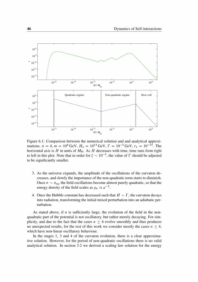
46 Dynamics of Self-interactions

H / MPl

r

1021 1018 1015 1012 109 106

1014

1012

1010

108

106

H / MPl

r

1021 1018 1015 1012 109 106

1014

1012

1010

108

106 Nonquadratic regime SlowrollQuadratic regime

Figure 6.1: Comparison between the numerical solution and and analytical approxi-mations. n D 4, m D 104 GeV, H� D 1013 GeV, � D 10�3 GeV, r� D 10�15. Thehorizontal axis is H in units of MPl. As H decreases with time, time runs from rightto left in this plot. Note that in order for � � 10�5, the value of � should be adjustedto be significantly smaller.

3. As the universe expands, the amplitude of the oscillations of the curvaton de-creases, and slowly the importance of the non-quadratic term starts to diminish.Once � � �eq, the field oscillations become almost purely quadratic, so that theenergy density of the field scales as �� / a�3.

4. Once the Hubble constant has decreased such thatH � � , the curvaton decaysinto radiation, transforming the initial mixed perturbation into an adiabatic per-turbation.

As stated above, if n is sufficiently large, the evolution of the field in the non-quadratic part of the potential is not oscillatory, but rather merely decaying. For sim-plicity, and due to the fact that the cases n � 6 evolve smoothly and thus producesno unexpected results, for the rest of this work we consider mostly the cases n � 4,which have non-linear oscillatory behaviour.

In the stages 1, 3 and 4 of the curvaton evolution, there is a clear approxima-tive solution. However, for the period of non-quadratic oscillations there is no validanalytical solution. In section 3.2 we derived a scaling law solution for the energy

6.2 Numerical Analysis 47

density of the curvaton when it is oscillating rapidly in a monomial potential. If thefield would be oscillating extremely fast compared to the background evolution, andthe amplitude of the oscillation would be very large, so that the non-quadratic termwould dominate the quadratic term for most of the oscillation, then this approximationwould be valid. These different phases and their approximations are demonstrated infigure 6.1. It illustrates clearly that while the oscillations in the quadratic regime arefast enough for the scaling solution to be a good approximation, for the non-quadraticregime the situation is not as evident.

Since the evolution of the self-interacting curvaton follows that of the quadraticcurvaton once the amplitude of the oscillations has decreased sufficiently, in prin-ciple the notation of section 4.3 is still valid. Thus the equations for �, fNL andgNL look deceivingly similar to the quadratic case. Even so, the non-linearity of theself-interacting model is merely hidden in the function �osc.��/, which evolves in anon-trivial, and as we shall see later on, oscillatory manner.

The approximative analysis stated above applies only for the homogeneous back-ground field value of the curvaton. For the quadratic model the homogeneous fieldvalue and the perturbation had the same (linear) equation of motion, so that the rel-ative perturbation stayed constant. In the non-quadratic case, the equation of motionfor the perturbation is very different,

Rı� C 3H Pı� C V 00.�/ ı� D 0 :

Now the evolution of the perturbations depends in a non-linear way on the evolutionof the background solution. Thus it is no longer sufficient to solve for the field valuewhen it decays, but rather we need to solve both the background EOM as well as theEOM for the perturbation. In practice it is usually simpler to use the �N -formalism,so that one does not need to solve the EOM for the perturbation separately, but ratherit is sufficient to solve the background equation multiple times.

6.2 Numerical Analysis

In the previous section we discussed analytical approximations for the self-interactingcurvaton scenario, in a similar fashion to what we did for the quadratic case in theprevious chapter. Be that as it may, due to the non-linearity of the self-interactingmodel we need to resort to numerical methods to take into account the evolution inthe non-quadratic part of the potential. Since we are solving the model numerically,we can also dispose of the other approximations we have made, most important ofthose being the instantaneous decay.

To compute the predictions of the self-interacting curvaton model of equation(5.9) numerically, we use the �N -formalism to compute the primordial perturba-tion amplitude and the corresponding non-Gaussianity parameters. The system of


equations that we need to solve is given by

R� C .3H C �/ P� Cm2� C .nC 4/�nC3

M nPl

D 0 ;

P�r D �4�r C � P�2 (6.1)3H 2M 2

Pl D �r C �� :

Also, the initial conditions are specified by the previously introduced two free param-eters, H� and r�, so that the initial energy densities are given by

�r D 3H 2�M

2Pl ;

�� D V.��/ D r��r :

The initial velocity of the curvaton field is assumed to be negligible, P�� D 0.Since when using the�N -formalism we are investigating differences in evolution

of two separate patches, we need to specify different initial conditions for the patches.In the other patch the initial conditions are given by the background, while the otherone has otherwise similar initial conditions, but the initial curvaton field value hasa small perturbation, originating from the quantum fluctuations described in section3.1,

�1 D �� ; �2 D �� CH�

2�:

The final amplitude of the primordial perturbation is then given by evolving the systemuntil the curvaton has decayed, and then comparing the number of e-folds in the twodifferent patches at a fixed value of H . In principle the full system, described bythe system of equations (6.1), should be used all the way until this final constantenergy density slice. Having said that, solving this set of differential equations isvery slow at the end of the simulation: As the field enters the quadratic regime, theoscillations become extremely rapid. Since several steps are needed for each cycle ofoscillation, the solution becomes increasingly slow to compute deep in the quadraticregime. To circumvent this, we use the fact that when the field is oscillating in aquadratic potential, in the limit of fast oscillations it satisfies a relation h

12

P�2i D

h12m2�2i, analogous to a harmonic oscillator. This means that in the limit of infintely

fast oscillations in the quadratic regime, the system has one degree of freedom less,and the behaviour of the curvaton field can be described perfectly by a single degreeof freedom, here chosen to be the energy density, �� . This energy density has thena well-behaving scaling law, �� / a�3. Thus after the quadratic term dominatessufficiently, 1

2m2�2 �

�nC4

MnPl

, we can safely switch to solving an approximate system,described by the equations

P�� D �.3H C �/�� ;

P�r D �4�r C �� ; (6.2)3H 2M 2

Pl D �r C �� :

6.3 Evolution of r 49

This corresponds to the approximation that the field is oscillating in a purely quadraticpotential very fast compared to the background solution. We have checked the numer-ical stability, and confirmed that the error created by this approximation is diminish-ingly small.

After the curvaton has decayed, we then calculate the difference of number ofe-folds in the two patches. This must be done in a uniform-density slicing, i.e., thetwo patches must be evolved to the same value of H . The difference in N in the twopatches is then directly �.

6.2.1 Non-Gaussianity

To compute the non-Gaussianity parameters in the �N -formalism, we use equations(4.5) and (4.6) where fNL and gNL are expressed as fractions of derivatives of thetotal number of e-folds with respect to the initial field value ��. Since numericalmethods have finite accuracy, the derivatives are calculated as finite differences. Thisis done using a numerical method called five-point stencil [52]. In this method, thederivatives of a function f .x/ are expressed as linear combinations of values of f .x/,different number of h-sized steps away from x. For fNL and gNL we need the threefirst derivatives, and these are given by the expressions

f 0.x/ D�f .x C 2h/C 8f .x C h/ � 8f .x � h/C f .x � 2h/

12h;

f 00.x/ D�f .x C 2h/C 16f .x C h/ � 30f .x/C 16f .x � h/ � f .x � 2h/

12h2;

f 000.x/ Df .x C 2h/ � 2f .x C h/C 2f .x � h/ � f .x � 2h/

2h3:

The five-point stencil has the advantage compared to many other finite differencemethods that the error made using these formulae is of order O.h4/.

For the calculation of the derivatives of N , we calculate the above expressionswith different values of the finite interval h, which is then adjusted dynamically tominimize the contribution of numerical noise and inaccuracy arising from the finite-ness of h.

6.3 Evolution of r

To gain some insight into the evolution of the self-interacting curvaton, it is oftenmore practical to follow the evolution of the energy fraction in the curvaton, definedby

r ��

�� C �r;

than the evolution of the field value �.t/. Indeed, since we solve the approximatesystem of equation (6.2) once we enter the quadratic regime, the field value is notalways uniquely determined by the program.


H / MPl

r

1020 1018 1016 1014 1012 1010 108

1011

1010

109

108

107

106

Figure 6.2: The evolution of the energy fraction r in time. H� D 10�7MPl, � D

10�2 GeV, n D 4 and r� D 10�14. The lower curve has the mass m D 104 GeV,whereas the upper curve has the mass m D 105 GeV. Note that for better visibility �has been set far too small to get � � 10�5.

As expected and already briefly discussed in section 6.1, the curvaton is initially inslow-roll and evolves slowly. Since � stays roughly constant, but the background ra-diation component dilutes as / a�4, r increases. After H has decreased sufficiently,the field, as well as the energy fraction r , starts to oscillate. As the field is still inthe non-quadratic part of the potential, the energy density of the curvaton scales downapproximately as calculated in section 3.2, that is, for n > 0 it dilutes faster thanthat of the background radiation, and thus r decreases. Note that since the oscilla-tions occur now in the non-quadratic regime, �� does not scale down smoothly, butwith an oscillatory envelope. After r and the field value of the curvaton have scaleddown sufficiently, the contribution of the non-quadratic term to the potential becomesnegligible, and the field starts to undergo almost purely quadratic oscillations. In thequadratic regime the equality h

12

P�2i ' h12m2�2i ' hV.�/i holds and the evolution

of r becomes smooth.

If the oscillations in the non-quadratic part of the potential would have a similar(short) period as the oscillations in the quadratic regime, the value of r would de-pend smoothly on the initial conditions. However, the periods differ by several ordersof magnitude. This causes the phase of the oscillation in the non-quadratic regimeto be frozen in when the oscillations change abruptly to quadratic oscillations. Thisis demonstrated in figure 6.2. Here the curvaton is evolved with otherwise similarparameters and initial conditions, but in the upper green line the mass has been cho-

6.4 Evolution of �N 51

sen to be 105 GeV, where as in the lower blue one it has been chosen to be 104 GeV.Since the mass determines when the transition from the non-quadratic to the quadraticregime occurs, the decrease of mass delays the transition a bit. However, as the os-cillations in the non-quadratic regime are quite slow, the transitions happen in com-pletely different phases of the oscillations: one at the top of an oscillation, while theother at the bottom of an oscillation. Since the initial conditions for the quadraticoscillations thus differ significantly, so do their later evolution: The curvaton whichswitched to the quadratic regime on the top of an oscillation has much larger value ofr later on than the curvaton which initiated its quadratic oscillations on the bottom ofan oscillation.

Note that in order for this effect to be significant, the regime of transition, thatis, the regime where both the quadratic and the non-quadratic term in the potentialare significant, must be shorter than the period of an oscillation in the non-quadraticregime. Otherwise the initial value for the quadratic oscillations would be an averageover several oscillations in the non-quadratic regime.

6.4 Evolution of �N

Although the non-quadratic oscillations can be slow when compared to the back-ground dynamics, the oscillations are nevertheless smooth: The evolution of r infigure 6.2 look quite close to a power law multiplied by some sinusoidal oscillation.However, we are not interested in the value of r , but rather the amplitude of the pri-mordial perturbations and the value of the non-Gaussianity parameters. In figure 6.3we have plotted the evolution of�N for a given set of parameters as a function ofH .Although the evolution of r is smooth, �N demonstrates very non-trivial behaviour.

There are several qualitative features manifest in figure 6.3. Firstly, the generalenvelope of the curve, averaged over the oscillations, follows approximately that ofr . This merely reflects equation (3.16), which states that the total perturbation, heregiven by �N , is the perturbation in � multiplied by the efficiency factor, which isroughly given by r . Thus the evolution of the general amplitude of�N , discarding theoscillatory features, is explained by the changes in the energy fraction in the curvaton:�N decreases in the non-quadratic regime as r decreases, and �N increases as thecurvaton starts to undergo quadratic oscillations and r starts to increase. Moreover,when the curvaton decays, the mixed perturbation in the curvaton is transformed intothe adiabatic perturbation of the total fluid, and thus�N freezes to its constant value.

The oscillations of�N are however more difficult to understand. The oscillationsin the non-quadratic regime appear very non-sinusoidal, as the full oscillation cycleconsists of two very different half-cycles. Again, since the evolution is very smoothin the quadratic regime, the value that �N has during the transition from the non-quadratic to the quadratic regime freezes in as the initial value for the quadratic evo-lution. Thus the final value of �N is very sensitive to the phase of the non-quadraticoscillations when the transition occurs.


H / MPl

|� N

|

10�20 10�18 10�16 10�14 10�12 10�10 10�8

10�13

10�12

10�11

10�10

10�9

Figure 6.3: Plot of the evolution of �N as a function of H . H� D 1013 GeV,m D

104 GeV, � D 10�3 GeV, n D 4, and r� D 10�15. Note that in order for � � 10�5,the value of � should be adjusted to be significantly larger.

Also noteworthy is the fact that though we actually plot j�N j due to the logarith-mic plot, the sign of �N actually oscillates: In the oscillations in the non-quadraticregime every other half-cycle of the oscillations has an opposite sign from its neigh-bouring half-cycles. Thus if the switch to the quadratic regime would occur duringa half-cycle with a negative sign, the final value of the perturbation would have anopposite sign to that of the initial perturbation. While this feature has no definiteobservational signature, it demonstrates the very counter-intuitive dynamics present:The patch which had initially higher energy density than the average, can have lowerenergy density in the final slice, and vice versa.

6.5 Oscillations in the Parameter Space

As demonstrated in the previous sections the long period of oscillations in the non-quadratic regime causes the phase of the non-quadratic oscillation to freeze in, so thatits value during the transition from the non-quadratic to the quadratic regime affectsthe final values of r and �N significantly. Thus any small change of parameterswhich affect either the phase of the non-quadratic oscillations or the point of transitionfrom the quadratic to the non-quadratic regime can change the final values by a largeamount.

Almost all of the parameters and initial conditions can affect the point of transitionand the phase of the non-quadratic oscillations: Sincem determines the value of �eq, it

6.5 Oscillations in the Parameter Space 53

r*

N'

10�22 10�20 10�18 10�16 10�14 10�12 10�10

�100�500

50100150

r*

N''

10�22 10�20 10�18 10�16 10�14 10�12 10�10

�5000000

0

5000000

r*

N'''

10�22 10�20 10�18 10�16 10�14 10�12 10�10�2e+11

�1e+11

0

1e+11

2e+11

Figure 6.4: N 0, N 00 and N 000 plotted against r�. The other parameters are given byn D 4, m D 106 GeV, and H� D 1012 GeV. The missing intervals in the plotscorrespond to those combinations of parameters which cannot produce � � 10�5.

also determines what is the value of H when the transition from the non-quadratic tothe quadratic regime occurs. r� plays the role of determining the initial homogeneousvalue of the field, ��. The initial amplitude of the perturbation is determined by H�.Different values of n corresponds to different behaviours in the non-quadratic regime.Thus if we would plot�N or its derivatives as a function of any of the forementionedparameters, we would see oscillatory behaviour.

In figure 6.4 we have plotted the values of N 0, N 00 and N 000 as a function of r� forfixed values of H�, m and n. Here the value of N 0 can be seen to have a nearly fixedmagnitude. This can be understood by N 0 approximately determining the amplitudeof the perturbation through the formula � ' N 0ı��. Since H� is fixed, so is ı��, andin order to get � � 10�5, N 0 must also have almost a fixed value. This is realized bytuning the value of � appropriately. N 0 nevertheless can change sign, and since ı��

is fixed, also � can change sign. Again, the sign of the primordial perturbation is not


0.1

1

10

100

1000

0.01 0.1 1

|f NL|

rdec

(a) jfNLj plotted against rdec for a fixed value of H� D 5 � 1012 GeV. Red pointscoresponds to fNL > 0 and blue points to fNL < 0.

0.1

1

10

100

1000

0.01 0.1 1

|f NL|

rdec

(b) jfNLj plotted against rdec for all values ofH� and r�.

Figure 6.5: The behaviour of jfNLj for a self-interacting curvaton model with n D 4

andm D 106 GeV. Only those points are plotted which produce the correct amplitudefor the perturbations in the range H� D 109 : : : 1013GeV and r� D 10�24 : : : 10�8.

observationally significant, but it does result in the counterintuitive result that patchesthat were overdense in the very early universe become underdense later on.

6.6 Comparison with the Analytical Estimates for fNL and gNL 55

0.1

1

10

100

1000

10000

100000

1e+06

0.1 1 10 100 1000 10000

g NL

fNL

Figure 6.6: jgNLj plotted against jfNLj for all values of H� and r� which producethe correct amplitude for the perturbations in the range H� D 109 : : : 1013 GeV andr� D 10�24 : : : 10�8. The green line corresponds to the linear relation gNL � fNLand the blue lines to the quadratic relation gNL � f 2NL. Other parameters are given byn D 4 and m D 106 GeV.

Even though � is adjusted so that N 0 does not oscillate, the same does not applyfor the higher derivatives: Both N 00 and N 000 oscillate wildly, also changing signs.This is a direct consequence of the slow non-quadratic oscillations. As r� is changed,the number of oscillations that the curvaton undergoes before the transition to thequadratic regime changes, and the phase of the non-quadratic oscillation freezes inproducing the observed oscillations of the derivatives of N as a function of the initialconditions.

6.6 Comparison with the Analytical Estimates forfNL and gNL

To demonstrate the non-linear and oscillatory behaviour of the self-interacting curva-ton, we compare the numerical results with the analytical expression calculated forfNL and gNL. In figure 6.5(a) the value of jfNLj is plotted against rdec for a fixed valueof H� and r� between 10�24 and 10�8 for m D 106 GeV and n D 4. In the figurewe can see the analytical estimate of equation (4.13) drawn as the black line, whereas


the red dots corresponds to the numerical results. From that we can see that while theanalytical expression for fNL roughly applies, the oscillations can signifcantly changethe value of fNL.

In figure 6.5(b) we have plotted all allowed points in the parameter space for amodel with m D 106 Gev and n D 4. As we allow H� to take different values, afamily of curves is drawn, where each curve is similar to the curve present in figure6.5(a), but each with a bit different oscillatory features, resulting into the noisy scatterpresent in the plot. Again we can see that the analytical result functions as an attractor,though most of the points are scattered aobve the line.

In figure 6.6 the value of jgNLj is plotted against the value of jfNLj. The green linecorresponds to the analytical expression for the quadratic curvaton in equation (4.13),and the blue line correponds to an analytical estimate for a non-quadratic curvaton inequation (4.14). We can see that there is a wide accumulation of points near the greenline, which corresponds to that area of the parameter space which is already initiallyin the quadratic regime. Similarly there appears to be a build-up of points near theblue line. In spite of that, most of the points are scattered around the plot.

Most points give rise to a larger fNL than one would expect from the analytical1=rdec-estimate, however since fNL can actually change sign, points can always befound where fNL is arbitrarily close to zero. It is also interesting to note that severaldifferent values of fNL correspond to a given point rdec, since different choices ofinitial conditions can be degenerate yielding the same rdec. It is also noteworthy thatfor a given fixed value of rdec, there are multiple sets of parameters which all give riseto the same final amplitude for the perturbations but different value of fNL and gNL.

Chapter 7

Results in theParameter Space

The numerical method described in the previous chapter can compute the amplitudeof the primordial perturbations, �, produced by a self-interacting curvaton for a set ofparameters fn;m;H�; r�; �g. To find out what combinations of the parameters canproduce perurbations compatible with observations, we first fix n and m, and thenscan through the parameter space spanned by H� and r�. We then impose constraintsto ensure that we are left with only those points in the parameter space which arecompatible with observations. The complete scan of the parameter space is performedin paper I and II, with the latter paper focusing on the non-Gaussianities created bythe self-interacting curvaton.

7.1 Allowed Regions of the Parameter Space

To make sure that the amplitude of the perturbations is correct we adjust the value ofthe effective decay constant � at each point in the .H�; r�/-space so that � � 10�5.Since decreasing � postpones the decay and thus makes the curvaton more dominant,smaller � translates to larger �. However, when the curvaton is already completelydominant when it decays, rdec � 1, decreasing � has no effect. Thus if � < 10�5 evenwhen rdec ' 1, then that point in the parameter space cannot produce the observedperturbations and thus that combination of the parameters is ruled out.

Note that the choice of which parameter to adjust while keeping the other param-eters fixed is not unique. Instead of adjusting � , we might just as well adjust r� to tryachieve the correct amplitude for �. Be that as it may, adjusting � is often easier, sincethe amplitude of � increases monotonously as a function of � , but not as a function ofr� etc.

As discussed in section 5.1, the curvaton must produce only adiabatic modes when

58 Results in the Parameter Space

it decays, and thus it must decay before dark matter decouples. By assuming that theDM particle is a generic WIMP, we get a lower limit for � (see section 5.1), whichdepends on the DM decoupling temperature. In papers I and II, we adopted the limit� > 10�15GeV, corresponding to a decoupling temperature TDM � O.GeV/, and inpaper III the more conservative limit � > 10�17GeV. Note that the choice of thelower limit is somewhat arbitrary, since it depends on the details of the DM model.We then discard those points in the parameter space which would require too small �to produce � � 10�5.

The curvaton can potentially produce non-Gaussianity so large that it would be inconflict with current observations, and thus those areas of the parameter space mustbe discarded. The current best observational limits are given in equations (4.2) and(4.3) [31, 76]. We thus compute the values of fNL and gNL for each point left in theparameter space, and discard those which produce non-Gaussianity incompatible withthe limits mentioned above.

The amount of tensor perturbations in the early universe is determined by theinflationary scale H�, and is not dependent on the field value of the inflaton. Thusobservations of the tensor modes would be a direct observation of the inflationaryscale. The observational limit for the tensor modes is usually given by the tensor-to-scalar ratio defined by

r �Pg.k/

PR.k/;

where Pg is the power spectrum for the tensor modes defined analogously with section2.4. The current best bounds for r are given by r < 0:36 from the CMB alone,or r < 0:20 where the CMB data is combined with data from baryonic acousticoscillations and supernovae observations [13]. The stricter value translates to a limitfor the inflationary scale

H� < 2:99 � 1014GeV :

To sum up, each point in the parameter space is evaluated with the followingcriteria:

1. There must be a value of � such that � � 10�5.

2. That value of � cannot be smaller than the limit given by the isocurvaturebound.

3. The non-Gaussianity parameters must be within observational limits, �9 <

fNL < 111 and �3:5 � 105 < gNL < 8:2 � 105.

4. The inflationary scale cannot be too large, as constrained by the tensor-to-scalarratio.

If the point in the parameter space passes all these tests, then we conclude that acurvaton model with that set of parameters could be responsible for the primordialperturbations that we observe.

7.2 Effect of Constraints in Parameter Space 59

1e-09 1e-08 1e-07 1e-06 1e-05 0.0001H*

1e-25

1e-20

1e-15

1e-10

1e-05

r *

b

a

c

d

Figure 7.1: A schematic plot of the effect of different constraints in the parameterspace. Line a is the bound imposed by limits on non-Gaussianity, line b demonstratesthe limit originating from the initial perturbation being smaller than 10�5, line c isthe requirement that the curvaton needs to be massless and very subdominant duringinflation, and line d is the isocurvature limit.

7.2 Effect of Constraints in Parameter Space

The different bounds originating from different observational limits mentioned in theprevious section make cuts in different regions of the parameter space. To illus-trate these different constraints and their effect in the allowed region of the parameterspace, we have plotted their effect schematically in figure 7.1.

The line a indicates the cut made by the observational limits for fNL and gNL. Inthe part of the parameter space dominated by the non-quadratic part of the potential,rdec increases from lower right to the upper left corner. Without the oscillations thenon-Gaussianity parameters would be given by roughly fNL / 1=rdec and gNL /

1=r2dec, and thus the cuts produced by these constraints would be direct lines in thedirection indicated by line a. However, due to the oscillations in the parameter space,both fNL and gNL increase un-monotonically as a function of rdec and thus the cutproduced by these constraints is not a straight line. Nevertheless, the parameter space


in the region indicated by the line a is mostly limited by non-Gaussianity.The cut indicated by line b is due to the initial perturbations in the curvaton field

being too small to evolve into the final perturbation of 10�5. If the homogeneouscurvaton field value and its perturbation would obey the same equation of motion, therelative perturbation would stay fixed all the way until decay, and then the amplitudeof the perturbation would be given by

� ' rdecH�

3��

:

The efficiency factor is given by rdec � 1, and thus if the initial perturbation givenby H�=2�� is smaller than the required �, then the curvaton cannot produce theobserved perturbations under any conditions. This limit would be given by a straightline such as the line b. However, the curvaton field value and its perturbation havedifferent equations of motion, and thus the final value of the relative perturbation isnot completely determined by the initial value, but instead is affected by the non-lineardynamics. Thus the cut is not given by a straight line, but rather by an oscillatorycurve.

The upper region of the parameter space is limited by several factors, indicated byline c. The higher the value of r�, the more massive the curvaton is during inflation.If the curvaton is too massive, it is no longer in slow-roll, but rather the value of thefield can change significantly during inflation. This would lead to a running of thespectral index, and thus we require that the curvaton is effectively massless duringinflation, V 00 � H 2

� . Note that since also the running of the inflaton and thusH� willalso produce running of the spectral index, we have not quantified this limit explicitly,as the exact limit will depend on the details of the inflationary model [101]. It mighteven be possible to produce a model where with some fine-tuning the curvaton andthe inflaton would evolve appropriately to produce a scale invariant spectrum eventhough neither the inflaton nor the curvaton would be in slow-roll. Additionally thelimit indicated by line c also ensures that the perturbative treatment that we have usedis applicable: We have assumed that the curvaton is completely subdominant duringinflation and thus does not affect the dynamics of inflation. It is not completely clearwhat is the minimum requirement in order for this approximation to be consistent. Asufficient requirement is nevertheless given by r� � 1.

Finally the smooth cut in the lower left corner of the parameter space is givenby the isocurvature limit, i.e., a lower limit on the magnitude of the effective decayconstant � . This limit is demonstrated by the line d.

7.3 Scan of the Parameter Space

A thorough scan of the parameter space was performed in articles I and II. We con-sidered values of n from 0 to 6 and values of m from 106GeV to 1010GeV. We thenscanned through the parameter space of .H�; r�/ for all combinations of m and n.

7.4 The TeV-mass Curvaton 61

The numerical results confirm the qualitative understanding of the oscillationspresented in chapter 6. From the plots in article I we see that for n D 6 there areno oscillations in the non-quadratic regime of the potential, and thus there are nooscillations either in the parameter space. Also for n D 0 the oscillations are so rapidin the non-quadratic part, that the phase thereof does not freeze in but rather is wipedout by the transition from the non-quadratic regime to the quadratic regime. Here thetransition lasts several oscillation cycles.

For n D 2 and n D 4 the oscillations in the non-quadratic potential result in largeoscillations in the parameter space. The values of � , rdec, fNL and gNL all oscillate, orare strongly dependent on small alterations of the initial conditions. These oscillationsresult in such regions in the parameter space being allowed, which would seem to bedisallowed by naıve analysis. Specifically, since both fNL and gNL oscillate, even inareas where the analytical approximations would give large values for fNL and gNL,there are always points where at least the other one is zero. The observational limitsfor gNL are much less stringent than for fNL, and thus points around fNL � 0 areusually allowed.

In general the results of article II indicate that there is not much parameter spaceleft for the n D 0 case.1 Instead, for n D 2, 4 and 6 there are large areas in theparameter space which are compatible with observations. Since fNL and gNL oscillatewildly, their absolute magnitude is nevertheless large in most of the allowed regions.Large non-Gaussianity here of course means allowed by observations but significantlynon-zero, and perhaps detectable with next generation CMB experiments, such asPlanck.

The values of the decay constant � mostly populate the lower limit imposed bythe isocurvature bound. A priori this of course is not a nuissance, however, one canargue that the model implies fine tuning if the curvaton is required to decay just beforeDM decoupling. The small values of � can also be a problem for a model builder,since this suggests very small coupling costants.

7.4 The TeV-mass Curvaton

There are strong theoretical hints that there may be significant new physics on the TeVscale. Furthermore current and future experiments, such as the LHC, might discovernew degrees of freedom which might function as a curvaton field [102]. Thus inarticle III we took the parameter choice m D 1 TeV as a specific example.

As demonstrated in section 5, for a curvaton with a TeV mass, the assumptionof a quadratic potential is not self-consistent, since even the weak self-interactionsof equation (5.9) will always play a significant role in the evolution of the curvaton.Furthermore, we found that even though a priori unconstrained, n can take only the

1Note that since we chose the potential to have the form of equation (5.9), the n D 0 corresponds toa very strong coupling. If one would add a small coupling constant, then this would leave more parameterspace allowed.


value n D 4. This is due to the fact that for other choices of n the curvaton needs todecay so late that the isocurvature limit rules these scenarios out, and only the n D 4

potential offers sufficient amplification of the perturbations due to the non-linearitiesso that all constraints are satisified. The part of the parameter space which is allowedfor n D 4 is then limited to isolated stripes in the .H�; r�/-space. Their total area issmall compared to the total parameter range, but still sufficiently large.

The TeV mass curvaton requires values for � that are very close to the lower limitimposed by the isocurvature bound. Though this is not a problem for the curvatonmodel in general, it is a problem for most realistic particle physics motivated models.One of the most attractive candidates of scalar fields to function as the curvaton arethe flat directions present in supersymmetric theories. Specifically, the widely studiedMinimally Supersymmetric Standard Model, or MSSM, which is one of the mostpopular candidates for extensions of the Standard Model, feature a large number ofthese flat directions (for a review, see e.g. [103] and references therein). These flatdirections have usually self-interactions of the form of equation (5.9), and thus areviable candidates for a curvaton scenario. Indeed, MSSM flat directions have beensuggested to work as a curvaton previously [104–109]. Nevertheless, the values ofdecay constant found in article III are very small, since the couplings that they applyare smaller than the couplings present in the Standard Model, and thus also in theMSSM.

7.4.1 Additional Mechanisms to Facilitate Small Values of �

If the actual couplings are larger than suggested by the numerical values of � found inthe scan of the parameter space, than additional mechanisms are required to explainwhy the curvaton decays so late.

One of the possibilites is so called kinematic blocking. Here the idea is that thefields to which the curvaton is supposed to decay acquire an effective mass that ispropotional to the coupling constant and the VEV of the curvaton. If the curvaton hasa sufficiently large VEV, than it might be that the would-be decay products have sucha large mass that the process of the curvaton decay to the other particles might bekinematically blocked. A real field oscillating around its minimum always of coursepasses through zero, and thus the VEV of the field also goes to zero. Thus kine-matic blocking is possible only if the oscillating field is complex. Though the anal-ysis present in this work concerns only real fields, in the article III we argue thatif a complex field is oscillating around its minimum with sufficiently small angularmomentum, the dynamics that it experiences are very similar to those experiencedby a real field. Thus the small effective value of � might be explained by the decaychannels of the curvaton being kinematically blocked. In the cases where the curvatonfield oscillates near zero preheating type phenomena will, however, become important[105, 110–112].

Also note, that what matters is not really where the energy density is, e.g. in thecurvaton or in the background, but rather the equation of state of the energy compo-

7.4 The TeV-mass Curvaton 63

nent. Thus, if the curvaton decays into an energy component which has the equationof state of matter, then this effectively delays its decay. One such possibility is Q-balls[113, 114] which are macroscopic exitations of complex scalar fields. A collection ofQ-balls would have the correct equation of state, w D 0, and as the Q-balls decaythrough surface evaporation, the decay into radiation can be delayed [115, 116].


Chapter 8

Conclusions

In this thesis we have studied the ability of curvaton models to produce the primordialperturbations. Specifically we have documented the behaviour and dynamics of self-interacting curvaton models, and discussed the allowed regions in the parameter spaceof these models.

It seems plausible that the curvaton, like any other scalar field, has some self-interactions. The type of self-interactions that we consider here has the most simplestfunctional form imaginable, that is, a monomial. Furthermore, we assume that themass scale suppressing the self-interaction is the Planck scale, i.e., the highest scalewhere “conventional” physics is thought to apply, and thus the self-interaction is veryweak. In this sense our assumption on the form of the self-interaction is very minimaland well motivated.

As discussed in [86–89, 97, 107, 111, 117, 118], even small deviations from theextensively studied quadratic potential [80] can cause significant effects. In fact, eventhe type of potential that we consider has been studied for example in [107]. Never-theless, we have presented for the first time thorough analysis of the dynamics of theself-interacting model. The crucial ingredient for this compared to the previous workwas the numerical solution of the equations of motion. In fact, the interesting oscilla-tory features are completely absent when modeling the evolution of the curvaton withapproximative scaling laws.

The self-interactions of the model affect the dynamics of the system in much moredrastic ways than one would suspect after naıve analysis: The non-linearity introducedby the self-interactions changes drastically the predictions of the self-interacting cur-vaton models in wide regions in the parameter space. The slow oscillations in thenon-quadratic part of the potential cause the phase of those oscillations to be frozenin to the final value of � and derivatives of N , and thus cause oscillations in the pa-rameter space.

The oscillatory behaviour caused by the self-interaction produces also typicallylarge values of fNL and/or gNL. This is caused by the oscillatory behaviour of the

66 Conclusions

derivatives of N . Although the analytical results 1=rdec and 1=r2dec capture the non-Gaussianity originating from the subdominance of the curvaton during its decay,they fail to describe the non-Gaussianity originating from the oscillations in the non-quadratic part of the potential. Indeed, we have shown that the non-Gaussianity of thelatter type is usually the dominant contribution in the self-interacting models.

Even though the possible parameter space of the self-interacting curvaton modelis limited by several observational limits, there remains large regions in the parameterspace left for which a self-interacting curvaton would produce perturbations compat-ible with observations, with different combinations of n and m. For a curvaton witha mass of TeV scale we have shown that the only possible Planck suppressed mono-mial self-interaction has the power �8, since all other choices of n fail to produce theobserved perturbations.

The self-interacting curvaton scenario has several intersting properties that arequite rare in other inflationary scenarios. Since fNL and gNL oscillate, they can haveeither sign. In fact, since they oscillate there are regions in the parameter space wherefNL is negligible, and the dominant contribution to non-Gaussianity is given by gNL.(See also [87].)

The decay of the curvaton has not been studied in detail here, as we have merelyassumed that the decay processes are well described by an effective decay constant.The values of the decay constant are quite small, and imply weak couplings to knownphysics. Also preheating type phenomena related to the decay might play a significantrole and modify the results for e.g. non-Gaussianity significantly [105, 110–112].

A scenario with mixed perturbations from both the curvaton and inflaton or per-haps from multiple curvatons should be studied with these self-interactions in mind.Since the curvaton can produce (extremely) large values of fNL and gNL, one alterna-tive is that where as most of the amplitude of the perturbations might come from aninflaton with nearly Gaussian statistics, a very subdominant curvaton might produce asmaller perturbation component, but with such a large non-Gaussianity that the non-Gaussianity of the final perturbations might be dominated by the perturbations fromthe curvaton.

Bibliography

[1] K. Enqvist, S. Nurmi, G. Rigopoulos, O. Taanila, and T. Takahashi, TheSubdominant Curvaton, JCAP 0911 (2009) 003, [arXiv:0906.3126].

[2] K. Enqvist, S. Nurmi, O. Taanila, and T. Takahashi, Non-GaussianFingerprints of Self-Interacting Curvaton, JCAP 1004 (2010) 009,[arXiv:0912.4657].

[3] K. Enqvist, A. Mazumdar, and O. Taanila, The TeV-mass curvaton, JCAP1009 (2010) 030, [arXiv:1007.0657].

[4] R. A. Alpher, H. Bethe, and G. Gamow, The origin of chemical elements,Phys. Rev. 73 (1948) 803–804.

[5] B. Fields and S. Sarkar, Big-bang nucleosynthesis (PDG mini-review),astro-ph/0601514.

[6] G. Steigman, Primordial Nucleosynthesis: The Predicted and ObservedAbundances and Their Consequences, arXiv:1008.4765.

[7] G. Lemaitre, The expanding universe, Gen. Rel. Grav. 29 (1997) 641–680.

[8] A. A. Friedmann, Uber die Krummung des Raumes, Z. Phys. A. 10 (1922)377–386.

[9] H. P. Robertson, Kinematics and world-structure, Astrophys. J. 82 (1935) 284.

[10] H. P. Robertson, Kinematics and world-structure ii, Astrophys. J. 83 (1936)187.

[11] H. P. Robertson, Kinematics and world-structure iii, Astrophys. J. 83 (1935)357.

[12] M. Vardanyan, R. Trotta, and J. Silk, How flat can you get? A modelcomparison perspective on the curvature of the Universe, Mon. Not. Roy.Astron. Soc. 397 (2009) 431–444, [arXiv:0901.3354].

68 Bibliography

[13] E. Komatsu et. al., Seven-Year Wilkinson Microwave Anisotropy Probe(WMAP) Observations: Cosmological Interpretation, arXiv:1001.4538.

[14] E. Hubble, A relation between distance and radial velocity amongextra–galactic nebulae, Proc. Nat. Acad. Sci. 15 (1929) 168–173.

[15] R. H. Dicke, P. J. E. Peebles, P. G. Roll, and D. T. Wilkinson, CosmicBlack-Body Radiation, Astrophys. J. 142 (1965) 414–419.

[16] A. A. Penzias and R. W. Wilson, A Measurement of excess antennatemperature at 4080- Mc/s, Astrophys. J. 142 (1965) 419–421.

[17] C. L. Bennett et. al., 4-Year COBE DMR Cosmic Microwave BackgroundObservations: Maps and Basic Results, Astrophys. J. 464 (1996) L1–L4,[astro-ph/9601067].

[18] D. Baumann, TASI Lectures on Inflation, arXiv:0907.5424.

[19] A. H. Guth, The Inflationary Universe: A Possible Solution to the Horizon andFlatness Problems, Phys. Rev. D23 (1981) 347–356.

[20] A. A. Starobinsky, Spectrum of relict gravitational radiation and the earlystate of the universe, JETP Lett. 30 (1979) 682–685.

[21] A. A. Starobinsky, A new type of isotropic cosmological models withoutsingularity, Phys. Lett. B91 (1980) 99–102.

[22] A. R. Liddle, P. Parsons, and J. D. Barrow, Formalizing the slow rollapproximation in inflation, Phys. Rev. D50 (1994) 7222–7232,[astro-ph/9408015].

[23] P. J. Steinhardt and M. S. Turner, A Prescription for Successful New Inflation,Phys. Rev. D29 (1984) 2162–2171.

[24] D. S. Salopek and J. R. Bond, Nonlinear evolution of long wavelength metricfluctuations in inflationary models, Phys. Rev. D42 (1990) 3936–3962.

[25] A. R. Liddle and D. H. Lyth, COBE, gravitational waves, inflation andextended inflation, Phys. Lett. B291 (1992) 391–398, [astro-ph/9208007].

[26] D. H. Lyth and A. Riotto, Particle physics models of inflation and thecosmological density perturbation, Phys. Rept. 314 (1999) 1–146,[hep-ph/9807278].

[27] A. Vilenkin and L. H. Ford, Gravitational Effects upon Cosmological PhaseTransitions, Phys. Rev. D26 (1982) 1231.

[28] A. D. Linde, Scalar Field Fluctuations in Expanding Universe and the NewInflationary Universe Scenario, Phys. Lett. B116 (1982) 335.

Bibliography 69

[29] A. A. Starobinsky, Dynamics of Phase Transition in the New InflationaryUniverse Scenario and Generation of Perturbations, Phys. Lett. B117 (1982)175–178.

[30] T. S. Bunch and P. C. W. Davies, Quantum Field Theory in de Sitter Space:Renormalization by Point Splitting, Proc. Roy. Soc. Lond. A360 (1978)117–134.

[31] WMAP Collaboration, E. Komatsu et. al., Five-Year Wilkinson MicrowaveAnisotropy Probe Observations: Cosmological Interpretation, Astrophys. J.Suppl. 180 (2009) 330–376, [arXiv:0803.0547].

[32] WMAP Collaboration, J. Dunkley et. al., Five-Year Wilkinson MicrowaveAnisotropy Probe (WMAP) Observations: Likelihoods and Parameters fromthe WMAP data, Astrophys. J. Suppl. 180 (2009) 306–329,[arXiv:0803.0586].

[33] SDSS Collaboration, M. Tegmark et. al., Cosmological Constraints from theSDSS Luminous Red Galaxies, Phys. Rev. D74 (2006) 123507,[astro-ph/0608632].

[34] The 2dFGRS Collaboration, S. Cole et. al., The 2dF Galaxy Redshift Survey:Power-spectrum analysis of the final dataset and cosmological implications,Mon. Not. Roy. Astron. Soc. 362 (2005) 505–534, [astro-ph/0501174].

[35] S. Dodelson, Modern cosmology. Amsterdam, Netherlands: Academic Pr.(2003) 440 p.

[36] L. Sriramkumar, An introduction to inflation and cosmological perturbationtheory, arXiv:0904.4584.

[37] S. Matarrese, S. Mollerach, and M. Bruni, Second-order perturbations of theEinstein-de Sitter universe, Phys. Rev. D58 (1998) 043504,[astro-ph/9707278].

[38] H. Kurki-Suonio, “Cosmological Perturbation Theory.” 2007.

[39] J. M. Bardeen, P. J. Steinhardt, and M. S. Turner, Spontaneous Creation ofAlmost Scale - Free Density Perturbations in an Inflationary Universe, Phys.Rev. D28 (1983) 679.

[40] M. Sasaki, Large Scale Quantum Fluctuations in the Inflationary Universe,Prog. Theor. Phys. 76 (1986) 1036.

[41] V. F. Mukhanov, Quantum Theory of Gauge Invariant CosmologicalPerturbations, Sov. Phys. JETP 67 (1988) 1297–1302.

70 Bibliography

[42] D. Wands, K. A. Malik, D. H. Lyth, and A. R. Liddle, A new approach to theevolution of cosmological perturbations on large scales, Phys. Rev. D62(2000) 043527, [astro-ph/0003278].

[43] J. Garcia-Bellido and D. Wands, Metric perturbations in two-field inflation,Phys. Rev. D53 (1996) 5437–5445, [astro-ph/9511029].

[44] K. A. Malik and D. Wands, Gauge-invariant variables on cosmologicalhypersurfaces, gr-qc/9804046.

[45] A. J. Christopherson and K. A. Malik, The non-adiabatic pressure in generalscalar field systems, Phys. Lett. B675 (2009) 159–163, [arXiv:0809.3518].

[46] A. A. Starobinsky, Multicomponent de Sitter (Inflationary) Stages and theGeneration of Perturbations, JETP Lett. 42 (1985) 152–155.

[47] M. Sasaki and E. D. Stewart, A General analytic formula for the spectralindex of the density perturbations produced during inflation, Prog. Theor.Phys. 95 (1996) 71–78, [astro-ph/9507001].

[48] M. Sasaki and T. Tanaka, Super-horizon scale dynamics of multi-scalarinflation, Prog. Theor. Phys. 99 (1998) 763–782, [gr-qc/9801017].

[49] D. H. Lyth and D. Wands, Conserved cosmological perturbations, Phys. Rev.D68 (2003) 103515, [astro-ph/0306498].

[50] D. H. Lyth, K. A. Malik, and M. Sasaki, A general proof of the conservationof the curvature perturbation, JCAP 0505 (2005) 004, [astro-ph/0411220].

[51] G. I. Rigopoulos and E. P. S. Shellard, The Separate Universe Approach andthe Evolution of Nonlinear Superhorizon Cosmological Perturbations, Phys.Rev. D68 (2003) 123518, [astro-ph/0306620].

[52] M. Abramowitz and I. Stegun, eds., Handbook of Mathematical Functions.Dover Publications, 1972.

[53] M. S. Turner, Coherent Scalar Field Oscillations in an Expanding Universe,Phys. Rev. D28 (1983) 1243.

[54] K. Enqvist and M. S. Sloth, Adiabatic CMB perturbations in pre big bangstring cosmology, Nucl. Phys. B626 (2002) 395–409, [hep-ph/0109214].

[55] D. H. Lyth and D. Wands, Generating the curvature perturbation without aninflaton, Phys. Lett. B524 (2002) 5–14, [hep-ph/0110002].

[56] T. Moroi and T. Takahashi, Effects of cosmological moduli fields on cosmicmicrowave background, Phys. Lett. B522 (2001) 215–221,[hep-ph/0110096].

Bibliography 71

[57] A. D. Linde and V. F. Mukhanov, Nongaussian isocurvature perturbationsfrom inflation, Phys. Rev. D56 (1997) 535–539, [astro-ph/9610219].

[58] S. Mollerach, Isocurvature baryon perturbations and inflation, Phys. Rev.D42 (1990) 313–325.

[59] D. Langlois and F. Vernizzi, Mixed inflaton and curvaton perturbations, Phys.Rev. D70 (2004) 063522, [astro-ph/0403258].

[60] G. Lazarides, R. R. de Austri, and R. Trotta, Constraints on a mixed inflatonand curvaton scenario for the generation of the curvature perturbation, Phys.Rev. D70 (2004) 123527, [hep-ph/0409335].

[61] F. Ferrer, S. Rasanen, and J. Valiviita, Correlated isocurvature perturbationsfrom mixed inflaton- curvaton decay, JCAP 0410 (2004) 010,[astro-ph/0407300].

[62] T. Moroi, T. Takahashi, and Y. Toyoda, Relaxing constraints on inflationmodels with curvaton, Phys. Rev. D72 (2005) 023502, [hep-ph/0501007].

[63] K. Ichikawa, T. Suyama, T. Takahashi, and M. Yamaguchi, Non-Gaussianity,Spectral Index and Tensor Modes in Mixed Inflaton and Curvaton Models,Phys. Rev. D78 (2008) 023513, [arXiv:0802.4138].

[64] D. Langlois, F. Vernizzi, and D. Wands, Non-linear isocurvature perturbationsand non- Gaussianities, JCAP 0812 (2008) 004, [arXiv:0809.4646].

[65] H. Assadullahi, J. Valiviita, and D. Wands, Primordial non-Gaussianity fromtwo curvaton decays, Phys. Rev. D76 (2007) 103003, [arXiv:0708.0223].

[66] J. Valiviita, H. Assadullahi, and D. Wands, Primordial non-gaussianity frommultiple curvaton decay, arXiv:0806.0623.

[67] K. A. Malik, D. Wands, and C. Ungarelli, Large-scale curvature and entropyperturbations for multiple interacting fluids, Phys. Rev. D67 (2003) 063516,[astro-ph/0211602].

[68] E. Komatsu and D. N. Spergel, Acoustic signatures in the primary microwavebackground bispectrum, Phys. Rev. D63 (2001) 063002,[astro-ph/0005036].

[69] J. M. Maldacena, Non-Gaussian features of primordial fluctuations in singlefield inflationary models, JHEP 05 (2003) 013, [astro-ph/0210603].

[70] D. H. Lyth and Y. Rodriguez, The inflationary prediction for primordial non-gaussianity, Phys. Rev. Lett. 95 (2005) 121302, [astro-ph/0504045].

72 Bibliography

[71] N. Bartolo, E. Komatsu, S. Matarrese, and A. Riotto, Non-Gaussianity frominflation: Theory and observations, Phys. Rept. 402 (2004) 103–266,[astro-ph/0406398].

[72] D. Wands, Local non-Gaussianity from inflation, Class. Quant. Grav. 27(2010) 124002, [arXiv:1004.0818].

[73] C. T. Byrnes, S. Nurmi, G. Tasinato, and D. Wands, Scale dependence of localfNL, JCAP 1002 (2010) 034, [arXiv:0911.2780].

[74] C. T. Byrnes, M. Gerstenlauer, S. Nurmi, G. Tasinato, and D. Wands,Scale-dependent non-Gaussianity probes inflationary physics,arXiv:1007.4277.

[75] C. T. Byrnes, K. Enqvist, and T. Takahashi, Scale-dependence ofNon-Gaussianity in the Curvaton Model, arXiv:1007.5148.

[76] V. Desjacques and U. Seljak, Signature of primordial non-Gaussianity ofphi3-type in the mass function and bias of dark matter haloes, Phys. Rev. D81(2010) 023006, [arXiv:0907.2257].

[77] Planck Collaboration, Planck: The scientific programme,astro-ph/0604069.

[78] A. Slosar, C. Hirata, U. Seljak, S. Ho, and N. Padmanabhan, Constraints onlocal primordial non-Gaussianity from large scale structure, JCAP 0808(2008) 031, [arXiv:0805.3580].

[79] P. Creminelli and M. Zaldarriaga, Single field consistency relation for the3-point function, JCAP 0410 (2004) 006, [astro-ph/0407059].

[80] D. H. Lyth, C. Ungarelli, and D. Wands, The primordial density perturbationin the curvaton scenario, Phys. Rev. D67 (2003) 023503,[astro-ph/0208055].

[81] N. Bartolo, S. Matarrese, and A. Riotto, On non-Gaussianity in the curvatonscenario, Phys. Rev. D69 (2004) 043503, [hep-ph/0309033].

[82] C. Gordon and K. A. Malik, WMAP, neutrino degeneracy andnon-Gaussianity constraints on isocurvature perturbations in the curvatonmodel of inflation, Phys. Rev. D69 (2004) 063508, [astro-ph/0311102].

[83] K. A. Malik and D. H. Lyth, A numerical study of non-gaussianity in thecurvaton scenario, JCAP 0609 (2006) 008, [astro-ph/0604387].

[84] M. Sasaki, J. Valiviita, and D. Wands, Non-gaussianity of the primordialperturbation in the curvaton model, Phys. Rev. D74 (2006) 103003,[astro-ph/0607627].

Bibliography 73

[85] J. Valiviita, M. Sasaki, and D. Wands, Non-Gaussianity and constraints forthe variance of perturbations in the curvaton model, astro-ph/0610001.

[86] K. Enqvist and S. Nurmi, Non-gaussianity in curvaton models with nearlyquadratic potential, JCAP 0510 (2005) 013, [astro-ph/0508573].

[87] K. Enqvist and T. Takahashi, Signatures of Non-Gaussianity in the CurvatonModel, JCAP 0809 (2008) 012, [arXiv:0807.3069].

[88] Q.-G. Huang, Curvaton with Polynomial Potential, JCAP 0811 (2008) 005,[arXiv:0808.1793].

[89] P. Chingangbam and Q.-G. Huang, The Curvature Perturbation in theAxion-type Curvaton Model, JCAP 0904 (2009) 031, [arXiv:0902.2619].

[90] R. Bean, J. Dunkley, and E. Pierpaoli, Constraining Isocurvature InitialConditions with WMAP 3- year data, Phys. Rev. D74 (2006) 063503,[astro-ph/0606685].

[91] M. Kawasaki and T. Sekiguchi, Cosmological Constraints on Isocurvatureand Tensor Perturbations, Prog. Theor. Phys. 120 (2008) 995–1016,[arXiv:0705.2853].

[92] L. Bergstrom, Dark Matter Candidates, New J. Phys. 11 (2009) 105006,[arXiv:0903.4849].

[93] G. Steigman and M. S. Turner, Cosmological Constraints on the Properties ofWeakly Interacting Massive Particles, Nucl. Phys. B253 (1985) 375.

[94] M. Srednicki, R. Watkins, and K. A. Olive, Calculations of relic densities inthe early universe, Nucl. Phys. B310 (1988) 693.

[95] P. Gondolo and G. Gelmini, Cosmic abundances of stable particles: Improvedanalysis, Nucl. Phys. B360 (1991) 145–179.

[96] L. D. Duffy and K. van Bibber, Axions as Dark Matter Particles, New J. Phys.11 (2009) 105008, [arXiv:0904.3346].

[97] P. Chingangbam and Q.-G. Huang, New features in curvaton model,arXiv:1006.4006.

[98] K. Dimopoulos, Can a vector field be responsible for the curvatureperturbation in the universe?, Phys. Rev. D74 (2006) 083502,[hep-ph/0607229].

[99] M. Karciauskas, K. Dimopoulos, and D. H. Lyth, Anisotropic non-Gaussianityfrom vector field perturbations, Phys. Rev. D80 (2009) 023509,[arXiv:0812.0264].

74 Bibliography

[100] K. Dimopoulos, M. Karciauskas, and J. M. Wagstaff, Vector Curvaton withoutInstabilities, Phys. Lett. B683 (2010) 298–301, [arXiv:0909.0475].

[101] D. Wands, N. Bartolo, S. Matarrese, and A. Riotto, An observational test oftwo-field inflation, Phys. Rev. D66 (2002) 043520, [astro-ph/0205253].

[102] G. Kane, (ed. ) and A. Pierce, (ed. ), Perspectives on LHC physics, .Hackensack, USA: World Scientific (2008) 337 p.

[103] K. Enqvist and A. Mazumdar, Cosmological consequences of MSSM flatdirections, Phys. Rept. 380 (2003) 99–234, [hep-ph/0209244].

[104] S. Kasuya, M. Kawasaki, and F. Takahashi, MSSM curvaton in thegauge-mediated SUSY breaking, Phys. Lett. B578 (2004) 259–268,[hep-ph/0305134].

[105] R. Allahverdi, K. Enqvist, J. Garcia-Bellido, A. Jokinen, and A. Mazumdar,MSSM flat direction inflation: slow roll, stability, fine tunning and reheating,JCAP 0706 (2007) 019, [hep-ph/0610134].

[106] R. Allahverdi, K. Enqvist, A. Jokinen, and A. Mazumdar, Identifying thecurvaton within MSSM, JCAP 0610 (2006) 007, [hep-ph/0603255].

[107] K. Enqvist, A. Jokinen, S. Kasuya, and A. Mazumdar, MSSM flat direction asa curvaton, Phys. Rev. D68 (2003) 103507, [hep-ph/0303165].

[108] J. McDonald, Supersymmetric curvatons and phase-induced curvatonfluctuations, Phys. Rev. D69 (2004) 103511, [hep-ph/0310126].

[109] J. McDonald, Right-handed sneutrinos as curvatons, Phys. Rev. D68 (2003)043505, [hep-ph/0302222].

[110] G. N. Felder, L. Kofman, and A. D. Linde, Instant preheating, Phys. Rev. D59(1999) 123523, [hep-ph/9812289].

[111] K. Enqvist, S. Nurmi, and G. I. Rigopoulos, Parametric Decay of theCurvaton, JCAP 0810 (2008) 013, [arXiv:0807.0382].

[112] A. Chambers, S. Nurmi, and A. Rajantie, Non-Gaussianity from resonantcurvaton decay, JCAP 1001 (2010) 012, [arXiv:0909.4535].

[113] S. R. Coleman, Q Balls, Nucl. Phys. B262 (1985) 263.

[114] A. Kusenko and M. E. Shaposhnikov, Supersymmetric Q-balls as dark matter,Phys. Lett. B418 (1998) 46–54, [hep-ph/9709492].

[115] K. Enqvist, S. Kasuya, and A. Mazumdar, Inflatonic solitons in running massinflation, Phys. Rev. D66 (2002) 043505, [hep-ph/0206272].

Bibliography 75

[116] K. Enqvist, S. Kasuya, and A. Mazumdar, Adiabatic density perturbationsand matter generation from the MSSM, Phys. Rev. Lett. 90 (2003) 091302,[hep-ph/0211147].

[117] K. Dimopoulos, G. Lazarides, D. Lyth, and R. Ruiz de Austri, Curvatondynamics, Phys. Rev. D68 (2003) 123515, [hep-ph/0308015].

[118] M. Kawasaki, K. Nakayama, and F. Takahashi, Hilltop Non-Gaussianity,JCAP 0901 (2009) 026, [arXiv:0810.1585].

Documents

Primordial Perturbations from a Self-interacting Curvaton