Primer for the Inspection and Strength Evaluation · Primer for the Inspection and Strength Evaluation of Suspension Bridge Cables . 5. Report ... This Primer is intended to be a

Publication No. FHWA-IF-11-045May 2012

Primer for the Inspection and Strength Evaluation of Suspension Bridge Cables

U.S. Department of Transportation

Federal Highway Administration

Notice

This document is disseminated under the sponsorship of the U.S. Department of Transportation in the interest of information exchange. The U.S. Government assumes no liability for use of the information contained in this document. This report does not constitute a standard, specification, or regulation.

Quality Assurance Statement The Federal Highway Administration provides high-quality information to serve Government, industry, and the public in a manner that promotes public understanding. Standards and policies are used to ensure and maximize the quality, objectivity, utility, and integrity of its information. FHWA periodically reviews quality issues and adjusts its programs and processes to ensure continuous quality improvement.

Primer for the Inspection and Strength Evaluation

of Suspension Bridge Cables

Publication No. FHWA-IF-11-045

May 2012

Technical Report Documentation Page 1. Report No. FHWA-IF-11-045

2. Government Accession No.

3. Recipient’s Catalog No.

4. Title and Subtitle Primer for the Inspection and Strength Evaluation of Suspension Bridge Cables

5. Report Date May 2012 6. Performing Organization Code

7. Author(s) Brandon W. Chavel, Ph.D., P.E., and Brian J. Leshko, P.E.

8. Performing Organization Report No.

9. Performing Organization Name and Address HDR Engineering, Inc. 11 Stanwix Street, Suite 800 Pittsburgh, Pennsylvania 15222

10. Work Unit No. 11. Contract or Grant No.

12. Sponsoring Agency Name and Address Office of Bridge Technology Federal Highway Administration 1200 New Jersey Avenue, SE Washington, D.C. 20590

13. Type of Report and Period Covered Technical Report September 2007 – May 2012

14. Sponsoring Agency Code

15. Supplementary Notes FHWA Contracting Officer’s Technical Representative (COTR): Raj Ailaney, P.E. FHWA Contracting Officer’s Task Manager: Myint Lwin, P.E., S.E. 16. Abstract

This Primer is intended to be a practical supplement to NCHRP Report 534, Guidelines for Inspection and Strength Evaluation of Suspension Bridge Parallel Wire Cables, and FHWA Report No. FHWA-PD-96-001, titled Recording and Coding Guide for the Structure Inventory and Appraisal of the Nation’s Bridges. This Primer will serve as an initial resource for those involved in the inspection, metallurgical testing, and strength evaluation of suspension bridge cables in addition to providing necessary documentation for recording performed inspections, testing, and strength evaluations. Furthermore, this document is intended to provide field inspectors, technicians, and/or engineers with the necessary forms and information they need to perform an inspection. 17. Key Words Suspension Bridge, Bridge Cable, Inspection, Strength Evaluation, Bridge Cable Material Testing, NCHRP Report 534

18. Distribution Statement No restrictions. This document is available to the public through the National Technical Information Service, Springfield, VA 22161.

19. Security Classif. (of this report) Unclassified

20. Security Classif. (of this page) Unclassified

21. No of Pages

22. Price

Form DOT F 1700.7 (8-72) Reproduction of completed pages authorized

i

Primer for the Inspection and Strength Evaluation of Suspension Bridge Cables

Table of Contents FOREWORD .................................................................................................................................. 1

ACKNOWLEDGEMENTS ............................................................................................................ 2

1.0 Introduction ............................................................................................................................ 3

1.1 Documents ....................................................................................................................... 3

1.2 Primer Organization ......................................................................................................... 3

1.3 Suspension Bridge Cables................................................................................................ 4

1.3.1 Bridge Cable Components ...................................................................................... 5

1.3.2 Bridge Cable Protection .......................................................................................... 9

1.3.3 Causes of Cable Deterioration .............................................................................. 10

1.3.4 Cable Wire Corrosion ........................................................................................... 11

2.0 Inspection Guidelines and Laboratory Testing Methods ..................................................... 14

2.1 Cable Inspection............................................................................................................. 14

2.1.1 Levels of Inspection and Inspection Intervals ...................................................... 15

2.1.1.1 Inspections by Maintenance Personnel ............................................... 15

2.1.1.2 Biennial Inspections ............................................................................ 15

2.1.1.3 Internal Inspections ............................................................................. 21

2.1.2 Outline of Internal Inspections.............................................................................. 29

2.1.3 Outline of Inspection and Sampling ..................................................................... 30

2.1.4 Splicing of New Wires into the Cable .................................................................. 31

2.2 Cable Inspection............................................................................................................. 32

2.2.1 Tests of Wire Properties........................................................................................ 32

2.2.1.1 Specimen Preparation ......................................................................... 32

2.2.1.2 Tensile Tests ....................................................................................... 33

2.2.1.3 Obtaining Data for Stress vs. Strain Curves ....................................... 33

2.2.1.4 Fractographic Examination of Suspect Wires ..................................... 33

ii

2.2.1.5 Examination of Fracture Surface for Pre-existing Cracks .................. 34

2.2.2 Zinc Coating Tests ................................................................................................ 34

2.2.2.1 Weight of Zinc Coating ...................................................................... 35

2.2.2.2 Preece Test for Uniformity ................................................................. 35

2.2.3 Chemical Analysis ................................................................................................ 35

2.2.4 Corrosion Analysis................................................................................................ 36

3.0 Evaluation of Field and Laboratory Data overview ............................................................. 37

3.1 Mapping and Estimating Wire Deterioration ................................................................. 37

3.1.1 Number of Rings in the Cable .............................................................................. 37

3.1.2 Number of Wires in Each Ring ............................................................................. 38

3.1.3 Wire Deterioration/Corrosion Mapping ................................................................ 38

3.1.4 Fraction of Cable in Each Corrosion Stage........................................................... 40

3.1.5 Number of Broken Wires ...................................................................................... 41

3.2 Wire Properties .............................................................................................................. 42

3.2.1 Cracked Wires as a Separate Group ...................................................................... 42

3.2.2 Individual Wire Properties .................................................................................... 43

3.2.2.1 Mean Properties .................................................................................. 43

3.2.2.2 Minimum Properties in a Panel Length .............................................. 44

3.2.3 Wire Group Mean Strength and Standard Deviation ............................................ 45

3.3 Wire Redevelopment ..................................................................................................... 45

4.0 Estimation of Cable Strength ............................................................................................... 46

4.1 Wire Groupings .............................................................................................................. 47

4.2 Strength of Unbroken Wires .......................................................................................... 47

4.2.1 Simplified Strength Model .................................................................................... 47

4.2.1.1 Mean Tensile Strength of Uncracked Wires ....................................... 48

4.2.1.2 Cable Strength Using the Simplified Model ....................................... 48

4.2.2 Brittle-Wire Strength Model ................................................................................. 49

4.2.3 Limited Ductility Strength Model ......................................................................... 50

4.3 Non-applicability of Load and Resistance Factor Rating (LRFR) ................................ 51

5.0 Inspection Documentation, Reporting, and Recommendations ........................................... 52

5.1 Maintenance Personnel Inspection Reports ................................................................... 52

iii

5.2 Biennial Inspection Report ............................................................................................ 52

5.3 Internal Inspection Report.............................................................................................. 53

6.0 References ............................................................................................................................ 55

7.0 Appendix A: Strength Evaluation Example ........................................................................ 56

7.1 Prior to Inspection .......................................................................................................... 57

7.1.1 Number of Wires in the Cable .............................................................................. 57

7.1.2 Number of Rings in the Cable .............................................................................. 57

7.1.3 Number of Wires in Each Ring ............................................................................. 59

7.2 Analyzing Inspection Data ............................................................................................. 60

7.2.1 Corrosion Map ...................................................................................................... 63

7.2.2 Broken and Removed Wires for Testing .............................................................. 64

7.2.3 Number of Wires in Each Corrosion Stage ........................................................... 65

7.3 Analyzing Laboratory Testing Data ............................................................................... 69

7.3.1 Test data for Wire Number 609 ............................................................................ 69

7.3.2 Test Data for Wire Number 613 ........................................................................... 71

7.3.3 Summary of all Test Data ..................................................................................... 72

7.3.4 Cracked Wires as a Separate Group ...................................................................... 75

7.4 Cable Strength Evaluation – Simplified Model ............................................................. 75

7.4.1 Estimate of Number of Broken Wires in the Development Length (Panel) ......... 76

7.4.2 Cracked Wires in the Evaluated Panel .................................................................. 77

7.4.3 Estimate of Cable Strength ................................................................................... 78

8.0 Appendix B: Previous Inspection References ..................................................................... 82

9.0 Appendix C: Flowcharts ..................................................................................................... 83

9.1 Inspection Flowchart ...................................................................................................... 83

9.2 Strength Evaluation Flowchart ...................................................................................... 84

10.0 Appendix D: Inspection and Evaluation Forms .................................................................. 85

10.1 Inspection Forms ............................................................................................................ 85

10.2 Strength Evaluation Forms ............................................................................................ 93

11.0 Appendix E: BTC Method for Evaluation of Remaining Strength and Service Life of

Bridge Cables ................................................................................................................................ 98

11.1 Introduction .................................................................................................................... 98

iv

11.2 Main Cable Inspection and Sampling ............................................................................ 99

11.2.1 Panel Selection Criterion ...................................................................................... 99

11.2.2 Random Sampling and Sample Size Determination ............................................. 99

11.2.2.1 Random Sampling and Practical Considerations .............................. 100

11.2.2.2 Sampling Size Determination ........................................................... 100

11.2.2.3 Wedge Pattern ................................................................................... 101

11.2.2.4 Sampling Frame of Random Sample ................................................ 101

11.2.3 Inspection Procedures ......................................................................................... 102

11.3 Wire Testing Program .................................................................................................. 104

11.3.1 Enhanced Tensile Strength Test in Standard Wire Specimens ........................... 104

11.3.2 Tensile Strength Test on Long Wire Specimens ................................................. 104

11.3.3 Fracture Toughness Test ..................................................................................... 104

11.3.4 Fractographic and Scanning Electron Microscope (SEM) Evaluation ............... 105

11.4 Cable Strength Evaluation ........................................................................................... 105

11.4.1 BTC Method Inputs ............................................................................................ 105

11.4.2 Choice of Probability Distributions .................................................................... 106

11.4.3 Elongation Threshold Criterion, Mthreshold ........................................................... 106

11.4.4 Determination of Wire Condition ....................................................................... 107

11.4.5 Wire Recovery Length ........................................................................................ 107

11.4.6 Broken Wires ...................................................................................................... 108

11.4.6.1 Exterior Broken Wires ...................................................................... 108

11.4.6.2 Interior Broken Wires ....................................................................... 109

11.4.7 Cracked Wires ..................................................................................................... 109

11.4.8 Strength Evaluation using the BTC Method ....................................................... 109

11.5 BTC Method Forecast of Cable Life ........................................................................... 109

11.5.1 Forecast of Degradation in Intact Wire Strength ................................................ 110

11.5.2 Forecast of Degradation in Cracked Wire Strength ............................................ 110

11.6 Sensitivity Analysis ..................................................................................................... 111

11.6.1 Key Inputs ........................................................................................................... 111

11.6.2 Sensitivity Indices ............................................................................................... 112

11.7 Appendix E References................................................................................................ 112

v

vi

List of Figures

Figure 1-1 Drawing showing an elevation view of a typical suspension bridge (taken from

NCHRP Report 534) .................................................................................................. 4

Figure 1-2 Drawings showing an elevation and cross-sectional view of a typical tower saddle

(taken from NCHRP Report 534) .............................................................................. 6

Figure 1-3 Drawing showing an elevation view of a cable anchorage (taken from NCHRP Report

534) ............................................................................................................................ 7

Figure 1-4 Drawing showing an elevation view of cable bent saddle (taken from NCHRP Report

534) ............................................................................................................................ 7

Figure 1-5 Photo showing a clamping collar and splay casting...................................................... 8

Figure 1-6 Photo showing a cable band with no suspenders .......................................................... 9

Figure 1-7 Photo showing a cable band with suspenders ............................................................... 9

Figure 1-8 Inspection photo showing small perforations in the cable wrap which is a potential

water ingress location .............................................................................................. 11

Figure 1-9 Photographs showing the four stages of cable wire corrosion [taken from [5]] ......... 12

Figure 1-10 Photographs showing local pitting corrosion and pitting with localized exfoliation of

iron oxide [taken from [5]] ...................................................................................... 13

Figure 2-1 Drawing of a three-span suspension bridge highlighting various components (taken

from BIRM [3])........................................................................................................ 14

Figure 2-2 Typical cable biennial inspection form (taken from NCHRP Report 534) ................. 17

Figure 2-3 Drawing showing a protective sleeve adjacent to tower saddle (taken from NCHRP

Report 534) .............................................................................................................. 18

Figure 2-4 Drawing showing an elevation view and cross-section of a typical cable band (taken

from NCHRP Report 534) ....................................................................................... 18

Figure 2-5 Drawing showing the typical components of an anchor block (taken from BIRM [3])

.................................................................................................................................. 19

Figure 2-6 Typical cable inside anchorage biennial inspection form (taken from NCHRP Report

534) .......................................................................................................................... 20

Figure 2-7 Form for recording defects in the suspender cable system (taken from BIRM [3]) ... 21

Figure 2-8 Photo showing damaged caulking and paint at a cable band (taken from NCHRP

Report 534) .............................................................................................................. 23

vii

Figure 2-9 Photo showing a ridge which indicates crossing wires (taken from NCHRP Report

534) .......................................................................................................................... 23

Figure 2-10 Photo showing a hollow area which indicates crossing wires (taken from NCHRP

Report 534) .............................................................................................................. 24

Figure 2-11 Form for recording locations of internal cable inspections (taken from NCHRP

Report 534) .............................................................................................................. 25

Figure 2-12 Form for recording observed wire damage inside the wedged opening (taken from

NCHRP Report 534) ................................................................................................ 27

Figure 2-13 Form for recording locations of broken wires and samples for testing (taken from

NCHRP Report 534) ................................................................................................ 28

Figure 2-14 Photo showing a typical cable wedged open for inspection (taken from NCHRP

Report 534) .............................................................................................................. 29

Figure 2-15 Photograph of a cracked wire (taken from NCHRP Report 534) .............................. 34

Figure 3-1 Typical form for recording observed wire deterioration ............................................. 39

Figure 3-2 Typical wire deterioration/corrosion map ................................................................... 40

Figure 3-3 Graph for computing the inverse of the standard normal cumulative distribution

function (taken from NCHRP Report 534) .............................................................. 44

Figure 4-1 Graph for computing the strength reduction factor, K (taken from Figure 5.3.3.1.2-1

of NCHRP Report 534) ............................................................................................ 49

Figure 7-1 Drawing showing wires in half-sectors (taken from NCHRP Report 534) ................. 57

Figure 7-2 Drawing showing a cable divided into eight sectors (taken from NCHRP Report 534)

.................................................................................................................................. 58

Figure 7-3 Drawing showing field inspection data for the sector five wedged opening .............. 61

Figure 7-4 Drawing showing the cable wire corrosion map ......................................................... 63

Figure 7-5 Drawing showing the map of broken wires and wires removed for testing (taken from

NCHRP Report 534) ................................................................................................ 65

Figure 7-6 Graph for computing the inverse of the standard normal cumulative distribution ..... 71

Figure 7-7 Graph for computing the strength reduction factor, K (taken from Figure 5.3.3.1.2-1

of NCHRP Report 534) ............................................................................................ 80

Figure 10-1 Typical cable biennial inspection form (taken from Figure 2.2.3.1-1 of NCHRP

Report 534) .............................................................................................................. 85

viii

Figure 10-2 Typical summary form showing biennial inspection rating system (taken from

Figure 2.2.3.1-2 of NCHRP Report 534) ................................................................. 86

Figure 10-3 Typical form for biennial inspection showing detailed ratings (taken from Figure

2.2.3.1-3 of NCHRP Report 534)............................................................................. 87

Figure 10-4 Typical form for biennial inspection of cable inside anchorage (taken from Figure

2.2.3.2-1 of NCHRP Report 534)............................................................................. 88

Figure 10-5 Form for recording locations of internal cable inspections (taken from Figure

2.2.1.2.4-1 of NCHRP Report 534).......................................................................... 89

Figure 10-6 Form for recording observed wire damage inside wedged opening (taken from

Figure 2.3.1.2.4-2 of NCHRP Report 534) .............................................................. 90

Figure 10-7 Form for recording locations of broke wires and samples for testing (taken from

Figure 2.3.1.2.4-3 of NCHRP Report 534) .............................................................. 91

Figure 10-8 Form for recording cable circumference (taken from Figure 2.4.1-1 of NCHRP

Report 534) .............................................................................................................. 92

Figure 11-1 Eight-wedge pattern and pool of wire samples in the cable cross section .............. 101

Figure 11-2 Photo showing the sample tag in wedge #7, wedge #8 side, ring #4, panel point 3-4

................................................................................................................................ 102

Figure 11-3 Photo showing wedges driven to the center of the cable, interior broken wire is

shown ..................................................................................................................... 103

Figure 11-4 Photographs showing the four stages of corrosion ................................................. 104

ix

List of Tables

Table 2-1 Interval between internal inspections (taken from NCHRP Report 534) ..................... 22

Table 2-2 Sample lengths and number of specimens from each sample (taken from NCHRP

Report 534) ................................................................................................................ 32

Table 7-1 Number of wires in each ring ....................................................................................... 60

Table 7-2 Corrosion stages assigned to individual wires.............................................................. 62

Table 7-3 Number of wires in each corrosion stage ..................................................................... 68

Table 7-4 Results of tension tests for wire number 609 ............................................................... 70

Table 7-5 Results of tension tests for wire number 613 ............................................................... 72

Table 7-6 Summary of all tension test results ............................................................................... 73

Table 7-7 Cracked wires in the evaluated panel ........................................................................... 78

Table 7-8 Calculations for mean tensile strength of the cable ...................................................... 79

Table 10-1 Typical table that can be used for assignment of corrosion stages to individual rings

of wires ...................................................................................................................... 93

Table 10-2 Typical table that can be used for assignment of corrosion stages to half sectors of

cable ........................................................................................................................... 94

Table 10-3 Typical table that can be used to record tension test results for a single wire ........... 95

Table 10-4 Typical table that can be used to summarize the tension test results ......................... 96

Table 10-5 Typical table that can be used to summarize the number of broken and cracked wires

................................................................................................................................... 97

Table 10-6 Typical table that can be used for calculating the mean tensile strength ................... 97

1

FOREWORD The motivation for the development of the “Primer for the Inspection and Strength Evaluation of Suspension Bridge Cables” is to provide a practical supplement to the NCHRP Report 534, “Guidelines for Inspection and Strength Evaluation of Suspension Bridge Parallel Wire Cables,” and the FHWA “Recording and Coding Guide for the Structure Inventory and Appraisal of the Nation’s Bridges.” This Primer serves as an initial resource for planning and performing inspection, metallurgical testing, and strength evaluation of suspension bridge cables. This Primer also provides an example of a simplified strength evaluation, flowcharts illustrating the inspection and strength evaluation procedures, and inspection and strength evaluation forms that can be used, or replicated, by inspectors and engineers. Suspension bridges are significant investments in our nation’s infrastructure, in addition to serving as public lifelines. In many cases, suspension bridges are essential transportation links for regional, national, and international commerce. As these key infrastructure investments advance in age, there is a need to efficiently inspect and evaluate the strength of these bridges to ensure that they have adequate load-carrying capacity. Furthermore, bridge owners will desire to maintain and extend the service life of these bridge types based upon standardized inspections and strength evaluations. The Primer is expected to be of immediate interest to suspension bridge field inspectors, technicians, laboratory personnel, bridge engineers, and bridge owners. The constructive review comments on the final draft provided by many engineering professionals are very much appreciated. The readers of this Primer are encouraged to submit comments for enhancements of future editions of the Primer to Myint Lwin at the following address: Federal Highway Administration, 1200 New Jersey Avenue, S.E., Washington D.C. 20590.

M. Myint Lwin, Director

Office of Bridge Technology

2

ACKNOWLEDGEMENTS The authors would like to acknowledge the encouragement and guidance provided by Myint Lwin, the Director of the Office of Bridge Technology, and Raj Ailaney, the Contract Manager of the Office of Bridge Technology during the development of the Primer. The authors also would like to thank the engineering professionals that provided very useful review comments on the final draft of the Primer.

3

1.0 INTRODUCTION The intent of this Primer is to supplement NCHRP Report 534, Guidelines for Inspection and Strength Evaluation of Suspension Bridge Parallel Wire Cables (Mayrbaurl and Camo 2004) [1]1, and FHWA Report No. FHWA-PD-96-001, titled Recording and Coding Guide for the Structure Inventory and Appraisal of the Nation’s Bridges [2]. This primer will serve as an initial resource for those involved in the inspection, metallurgical testing, and strength evaluation of suspension bridge cables in addition to providing necessary documentation for recording performed inspections, testing, and strength evaluations. Furthermore, this document is intended to provide field inspectors, technicians, and/or engineers with the necessary forms and information they need to perform an inspection. 1.1 DOCUMENTS The Guidelines for Inspection and Strength Evaluation of Suspension Bridge Parallel Wire Cables, herein referred to as NCHRP Report 534, is an in-depth resource that can be used for assessing cable integrity through inspection, metallurgical testing, and strength evaluation. The Report also provides a method of standardization for the process of evaluating a cable that has been in service for an extended period of time. This Primer will highlight the critical aspects of cable inspection, laboratory testing, strength evaluation, and documentation of the entire process. Much of the information provided in this Primer is taken directly from the Report. However, for a more detailed treatment of the subjects contained in this Primer as well as additional topics, the reader is encouraged to review NCHRP Report 534. The Recording and Coding Guide for the Structure Inventory and Appraisal of the Nation’s Bridges provides detailed guidance in evaluating and coding specific bridge data that comprise the National Bridge Inventory database. This guide was developed for use by the states, federal and other agencies so as to have a complete and thorough inventory of the nation’s bridges. 1.2 PRIMER ORGANIZATION Section 2 of this Primer provides guidelines for inspecting suspension bridge parallel wire cables as detailed in NCHRP Report 534 and supplemented from Section 12, Special Bridges, Topic 12.1 Cable Supported Bridges in Publication No. FHWA NHI 03-001, Bridge Inspector’s Reference Manual [3]. Laboratory testing methods typically employed for suspension bridge parallel wire cables are as discussed in Section 2. An overview of the tabulation and presentation of field and laboratory observations is provided in Section 3. In Section 4, the methods that can be used to estimate the strength of the suspension cables are presented and discussed. These strength evaluation methods include the Simplified Model, the Brittle-Wire Model, and the Limited Ductility Model. Section 5 explains the documentation, reporting, and recommendations that should be created after the inspection and evaluation of a suspension bridge cable, which will allow owners to make informed decisions about maintenance schedules and budgets.

1 Numbers in brackets refer to References provided in section 6.0 of this document.

4

References are provided in Section 6, while Section 7 (Appendix A) contains an in-depth strength evaluation example using the Simplified Model. A list of references for inspection and evaluation projects that have employed the criteria of NCHRP Report 534 is provided in Section 8 (Appendix B). Section 9 (Appendix C) contains flowcharts demonstrating the processes for cable inspection and strength evaluation. Section 10 (Appendix D) includes blank forms that can be used by cable inspections, as well as tables that can be followed to perform strength evaluation calculations associated with the Simplified Model. Section 11 (Appendix E) presents the BTC Method, an alternative methodology to that provided in the NCHRP Report 534, for the assessment of remaining strength and residual life of bridge cables. The method applies to both; parallel and helical; either zinc-coated or bright wire suspension and cable-stayed bridge cables. The BTC method includes random sampling without regard to wire appearance, mechanical testing of wire samples, determining the probability of broken and cracked wires, evaluating ultimate strength of cracked wires employing fracture mechanics principles and utilizing the above data to assess remaining strength of the bridge cable in each panel. The probabilistic-based method forecasts remaining service life of the cable by determining the rate of growth in proportions of broken and cracked wires over a time frame, measuring the rate of change in effective fracture toughness over same time frame, and applying the rates of change to a strength degradation prediction model. The BTC method provides a sensitivity analysis to identify the key inputs which influence the estimated cable strength and assist in decision making regarding future maintenance. Persons interested in using the BTC method should contact the author of this Appendix. 1.3 SUSPENSION BRIDGE CABLES Suspension bridges are large, unique structures with two or more cables that carry the weight of the deck and the imposed live load to the towers that support the cables. The suspension cables are in tension and require massive anchorage at both ends, and are typically load-path nonredundant. Figure 1-1 shows an elevation view of a typical suspension bridge with main bridge components labeled.

Figure 1-1 Drawing showing an elevation view of a typical suspension bridge (taken from

NCHRP Report 534) The cables are constructed of many individual wires, typically laid parallel to one another and clamped at points where suspenders connect with them to support the bridge deck. For most North American bridges, these individual wires have a 0.192 inch diameter, and a 0.002 inch

5

zinc coating around the wire, resulting in a total diameter if 0.196 inch. Bridge cable wires are typically coated with zinc to provide cathodic protection to protect the wire steel against corrosion. The quality of the zinc coating is important to ensure wire safety; discontinuities produced during manufacturing or installation can facilitate corrosion of the steel wire. Suspension bridge cable wires are made of ultra high strength steels because of the heavy loads they are required to support. ASTM A586 mandates that the bridge cable wires are to have a minimum tensile strength of 220 ksi (kips per square inch). In some cases, modern wires exceed this specification with tensile strengths as high as 260 ksi. The requirement of 220 ksi strength is based on the gross metallic area, including the zinc coating. It should be noted that for the strength evaluation of older bridges, employing the methodology of this Primer and NCHRP Report 534, the above discussion concerning material properties may not be appropriate. In some cases, bridge cable wires may have a minimum tensile strength well below 220 ksi. The bridge engineer performing the inspection and evaluation must be aware of the original material specifications that may apply to the structure being investigated, or should otherwise have the particular component tested to determine necessary material properties. 1.3.1 Bridge Cable Components The performance of the bridge cable wires and their inspectability are affected by additional variables other than the cables themselves. Details such as tower saddles, cable bent saddles, splay castings, cable anchorages, and the connection of the suspenders to the cables can affect the performance and inspectability of the cable wires. The vertical forces at the top of the towers are transferred from the suspension bridge cable into the tower by the tower saddles. In most cases, the entire weight of the bridge is supported at the top of the tower. A typical tower saddle is shown in Figure 1-2.

6

Figure 1-2 Drawings showing an elevation and cross-sectional view of a typical tower

saddle (taken from NCHRP Report 534) Anchorage and cable bent saddles bend the suspension bridge cables so that they come into alignment with the anchoring mechanisms. Anchorage saddles sometimes have a variable vertical radius and horizontal flare, allowing the cable strands to be splayed directly to their anchoring mechanisms. A typical anchorage is shown in Figure 1-3. Cable bent saddles typically bisect the interior angle of the cable, so that the cable changes direction within a single vertical curve from the saddle toward the anchorage without flaring to a splay casting. Cable bent saddles are typically supported on independent struts that may be hinged at the base or, if flexible enough, fixed at the base. A typical cable bent saddle is shown in Figure 1-4.

7

Figure 1-3 Drawing showing an elevation view of a cable anchorage (taken from NCHRP

Report 534)

Figure 1-4 Drawing showing an elevation view of cable bent saddle (taken from NCHRP

Report 534) Splay castings, as shown in Figure 1-5, are used to control the direction of the strands that flare out of their respective anchoring devices. Castings resists the outward forces exerted by the strands, and are anchored against upward slippage by a cable collar clamped above the splay

8

casting. Corrosion of the wires inside the splay casting may be caused by water passing through the cable. However, inspecting wires inside the splay casting is a complex operation that typically requires a temporary relocation of the splay casting.

Figure 1-5 Photo showing a clamping collar and splay casting

Cable anchoring devices can consist of strand shoes, parallel wire strand terminations, or eyebars. Traditionally, cable wires loop around strand shoes, which are anchored to two eyebars by a pin. Alternatively, a single eyebar can be used with two strand shoes, one at each end of the pin, splitting the strand into four quarters. The strand shoe can also be restrained with high-strength strengthening rods. When a humid atmosphere exists in the anchorage or water enters the anchorage area, corrosion is often found in the lower half of the strands, particularly at the interfaces of the wires and the strand shoe where water tends to collect. Parallel wire strand terminations use zinc or polyester thermoset resin sockets rather than strand shoes, and the sockets are connected to anchoring assemblies embedded in the anchorage concrete. Eyebars are anchored to a grillage buried deep in the concrete mass of the anchorage. The focus of the eyebars may be slightly beyond the splay casting or cable bent saddle. To prevent eyebars from bending, spacers are placed between the eyebars of each separate strand so that the eyebars bear against each other. In humid anchorages, eyebar corrosion is typically found at the interface with the concrete mass, and is often hidden behind pack rust. Cable bands consist of two cylinder halves bolted together over the circumference of the cable. The number of bolts per cable band is dependent on the slope of the cable at the suspender attachment point. The friction from squeezing against the cable prevents the cable band from sliding down the cable. More bolts are needed as the cable becomes steeper to prevent the cable band from sliding. Figure 1-6 shows a cable band without suspenders attached, and Figure 1-7 shows a cable band with suspenders attached.

9

Figure 1-6 Photo showing a cable band with no suspenders

Figure 1-7 Photo showing a cable band with suspenders

The wires in a suspension cable are often protected by wire wrapping, which typically consists of soft galvanized No. 9 wires with Class A zinc coating. Some newer bridges have used an S-shaped wire that interlocks with the other wires. Wrapping is installed by power-driven machines with multiple reels that are capable of placing from one to three wires at a time. The wrapping wires are in a single layer, in side-by-side helices. Paint systems are used to cover and seal the wrapping wires. Other protection systems employ elastomeric membranes or fiberglass reinforced lucite composites and methacrylates. 1.3.2 Bridge Cable Protection The individual cable wires can be protected with the use of zinc coatings, grease and oil, and/or paste mixtures, while the complete suspension cable is typically protected with galvanized wire wrapping and paint. With few exceptions, the cable wires are protected with a zinc coating, which can last indefinitely or could become defective within 20 years depending on the effectiveness of the exterior protective system. The zinc coating provides cathodic protection,

10

and exploits the phenomenon of galvanic action to protect the steel against corrosion. In this application, the zinc coating provides cathodic protection by depleting in the presence of water thus protecting the steel. Some early bridge cable wires were greased during spinning or as the cable was being compacted. In some cases the greased wires have appeared almost new after many years of service and in other cases, despite the presence of grease, wires were known to crack and fail in localized zinc depleted regions. Furthermore, various paste mixtures were used as a layer of protection under wrapping wires to prevent water penetration. In the past, red lead paste was traditionally used under the wrapping wire; however, given the hazardous nature of red lead, zinc-based pastes have been used in Europe and the United States. Membrane protection and dehumidification are now widely used in Asia and have been used in Europe. 1.3.3 Causes of Cable Deterioration The deterioration of suspension bridge cable wires is principally caused by corrosion. Corrosion is caused by the presence of water and its solutes. There are several factors that affect a cable’s susceptibility to corrosion, including environmental aspects, amount of water penetration, installation practices, and the vulnerability of the wires to corrosion attack. The term macro-environment can be used to describe the environmental conditions that affect the structure as a whole. A suspension bridge’s macro-environment often contains moisture, pollutants, dissolved gases, and salt spray from deicing salts or coastal environment, all of which may contribute to corrosion of the cable wires. The term micro-environment can be used to describe the conditions inside the cable that affect the individual wires. Water can enter a cable as a liquid from either precipitation or as a vapor during periods of high temperature and humidity. The water vapor will turn to liquid form as the temperature falls, forming condensation on the wire surfaces. Some micro-environments, which can act alone or together, observed in bridge cables are:

• Acid rain chemistry, leading to hydrogen evolution from the reaction with the zinc wire coating

• Carbonate or bicarbonate chemistry, either alkaline or highly acidic • Nitrate chemistry, either alkaline or acidic • Alkaline chemistry • Seawater or salt spray, moderately acidic • Cathodic action in which a metal more noble than steel is placed in contact with the wires

These micro-environments can cause cable wires to corrode, crack, and/or break. There are several methods in which water can penetrate into the cable. A breakdown in the exterior protection system, such as poorly wrapped cables or cracks in the paint, can allow water to enter the cable. Furthermore, perforations can develop in the cable wrapping, as shown in Figure 1-8. Joints on the underside of the cable are often provided to allow for weeping of

11

internal water. However, these joints may become points of entry for water streaming along the underside of the cable or from wind-driven rain. Damaged or poorly maintained housings for saddles and anchorages can allow water to enter the cable or cause damage to the wires near the saddles and anchorages. Lastly, paint cracks and other entry points for water ingress are also entry points for water vapor, which can lead to condensation in the cables.

Figure 1-8 Inspection photo showing small perforations in the cable wrap which is a

potential water ingress location The cable installation practices can lead to deterioration of the wires. Poor cable compaction and crossing of the wires can cause unusually large voids in the cable that allow water to penetrate deep into the cable. The crossing of wires can also expose steel at the point of contact, and therefore accelerate cathodic action. The individual wires are more susceptible to corrosion than milled rolled steel due to the processes used to fabricate the wires, which includes a high carbon content and cold working of the steel. The zinc coating used to protect the wires from corrosion is beneficial as long as there are no breaches in the coating. If the zinc coating is damaged or missing, corrosion is more likely to occur. The “cast” of the wire, or its natural curvature (on the order of 4ft in diameter), which was necessary to initially spin the cables, has inherent high residual stress and very high straightening stresses predisposing the wires to be attacked in the inside radius of the wire. This is the foremost culprit in wire damage. Modern specifications call for as large of a “cast” as possible, where a diameter on the order of 30ft is possible. Wires manufactured with small cast radii have a high residual stress, estimated to be 30 to 36 ksi by X-ray diffraction. 1.3.4 Cable Wire Corrosion The corrosion mechanism for zinc-coated cable wires within the span is different than mechanisms for zinc-coated cable wires in the anchorages and for uncoated wires. The discussion that follows concerns cable wires within the span. Through visual inspection, wire corrosion is classified into four different stages, developed by Hopwood and Havens [4]. The classification system has over time provided accurate descriptions of the various stages of

12

corrosion in the cable wires, and produced a usable grouping for strength evaluation of the cable. As shown in Figure 1-9, the four stages of wire corrosion that are typically used are:

• Stage 1: white spots on the surface of the wire, indicating early stages of zinc oxidation • Stage 2: white zinc oxidation over the entire wire surface • Stage 3: white zinc oxidation in some areas of the wire, with brown rust spots not

covering more then 30% of a 3 in. to 6 in. length of wire • Stage 4: brown spots prevalent over the wire surface, covering more than 30% of a 3 in.

to 6 in. length of wire A 5th stage is often used as well, to represent wires that have stage 4 corrosion (above), but with cracks in the wires. A Stage 2 wire may have white surface dust, indicating zinc oxidation, but it does not necessarily imply depletion of the zinc coating. Depletion of the zinc coating is typically indicated by a dull gray color, or a dark gray to black color if sulfur is present.

Stage 1

Stage 2 Stage 3 Stage 4

Figure 1-9 Photographs showing the four stages of cable wire corrosion [taken from [5]] In addition to surface corrosion, pits of various types can be found in the wires. As shown in Figure 1-10, some Stage 4 wires can show extensive exfoliation and/or local pitting, or pitting characterized by highly localized exfoliation of iron oxide. Furthermore, laboratory tests have shown that 5% to 20% of Stage 3 corroded wires, and 60% of Stage 4 corroded wires, may have cracks.

13

Figure 1-10 Photographs showing local pitting corrosion and pitting with localized

exfoliation of iron oxide [taken from [5]]

14

2.0 INSPECTION GUIDELINES AND LABORATORY TESTING METHODS This section will discuss guidelines for inspecting suspension bridge parallel wire cables as detailed in NCHRP Report 534 and supplemented from Section 12, Special Bridges, Topic 12.1 Cable Supported Bridges in Publication No. FHWA NHI 03-001, Bridge Inspector’s Reference Manual (BIRM) [3]. Laboratory testing methods and results, used to estimate wire strength and ultimately evaluate cable strength, will also be highlighted herein. 2.1 CABLE INSPECTION A typical suspension bridge is comprised of a deck system that is connected by vertical suspender cables to the main suspension cables, which are generally supported on saddles atop towers and are anchored at both ends. Figure 2-1 depicts a three-span suspension bridge schematic, identifying these major components. Suspension bridges with only two main suspension cables offer only two load paths (non-redundant); therefore, the two tension cables are identified as fracture critical members for the purpose of inspection and evaluation.

Figure 2-1 Drawing of a three-span suspension bridge highlighting various components

(taken from BIRM [3]) The goal of the cable inspection is to obtain information about the condition and strength of the cable wires, which can then be used to evaluate suspension bridge cable strength. Although several levels of inspection are performed over the lifespan of the structure, only internal cable inspections provide data for strength evaluation. Cable inspections should be led by a chief inspector, a professional engineer with experience in bridge cable inspections. Cable inspection over trafficked roadways and waterways involves risk to people and the environment. Protection of construction workers, inspectors, motorists, pedestrians, and marine traffic is an important consideration. Personnel associated with the cable inspection should understand health hazards and be trained in the use of equipment (full-body safety harness, dual shock-absorbing lanyards, etc.) and monitoring procedures (blood-lead baseline and subsequent checks for lead absorption) associated with health maintenance.

15

Reference the OSHA Compliance Manual Training requirements and Subsection 1.2 Health and Safety Requirements of NCHRP Report 534. 2.1.1 Levels of Inspection and Inspection Intervals There are three levels of cable inspection:

• Periodic routine visual inspections by maintenance personnel of the cable exterior • Biennial hands-on inspections of non-redundant members • Scheduled thorough internal inspections

2.1.1.1 Inspections by Maintenance Personnel Periodic inspection tours of the cable by maintenance personnel are recommended, beginning by inspecting the underside of the cable with binoculars, and then walking the cable along its full length. These inspections should occur at the end of winter (March or April) to observe damage due to frost or deicing salts in the splash zone, and at the end of summer (September or October) to observe the effects of extreme heat on paint and caulking. Additional inspections should occur after severe snow, ice, rain or wind storms. During these inspections, the underside of the cable should be examined for evidence of water penetration (dripping from the wrapping wire or weep holes in the lower cable band grooves, and unusually damp areas). 2.1.1.2 Biennial Inspections In accordance with the National Bridge Inspection Standards (NBIS), non-redundant fracture critical members receive hands-on inspections every 24-months. Suspension bridges are considered complex bridges according to the NBIS regulations. The NBIS requires identifying specialized inspection procedures, and additional inspector training and experience to inspect these complex bridges. Suspension bridges are to be inspected according to these procedures. Specifically developed bridge maintenance manuals, if available, should be used to verify that specified routine maintenance has been performed. Customized, preprinted inspection forms should be used to report findings in a systematic manner. Cables in Suspended Spans: Inspect the main suspension cables for indications of corroded wires. Inspect the protective covering or coating, especially at low points of cables, areas adjacent to the cable bands and saddles over towers. The conditions of the following bridge components should be reported (see Figure 2-2 for sample form):

• Paint or Surface Protection, inspected for dried out, peeling, cracked and crazed paint • Elastomeric Barrier (see Figure 2-3), inspected for puncture or tearing • Caulking at Cable Bands, inspected for gaps or cracks • Hand Ropes and Stanchions, inspected for broken wires, tightness and corrosion • Wire Wrapping, inspected for anomalies including:

o Unequal tension of wire plies, indicated by unevenness in wrapping surface o Bunching below or separating above the cable bands o Gaps in wrapping, corroded or broken wrapping wire o Surface ridges, indicated by crossing wires and hollow areas

16

• Saddles, inspected for missing or loose bolts, damaged sleeves, bellows or flashing, and corrosion or cracks in the casting. Check for proper connection to top of tower or supporting member, and possible slippage of the main cable.

• Cable Bands (see Figure 2-4), inspected for missing or loose bolts, rust stains or dripping water, indicative of internal corrosion, or broken suspender saddles. Check for the presence of cracks in the band itself as well as corrosion or deterioration of the band.

• Measure and report the cable diameter at several intervals along the cable. Later, the diameter of the cable in combination with the known number of wires, can be used to estimate the potential for water accumulation.

17

Figure 2-2 Typical cable biennial inspection form (taken from NCHRP Report 534)

18

Figure 2-3 Drawing showing a protective sleeve adjacent to tower saddle (taken from NCHRP Report 534)

Figure 2-4 Drawing showing an elevation view and cross-section of a typical cable band

(taken from NCHRP Report 534)

19

Cables Inside Anchorages: Inspect the anchorage system (see Figure 2-5 for schematic of components) at the ends of the main suspension cables. The splay saddle, bridge wires, strand shoes or sockets, anchor bars, and chain gallery need to be inspected. The conditions of the following bridge components should be reported (see Figure 2-6 for sample form):

• Strands Inside Anchorages, inspected for corrosion or broken wires, and swelling or bulges at the strand shoes

• Anchorage Walls and Roof (Chain Gallery), inspected for signs of water intrusion • Eyebars and Strand Wires, inspected for signs of condensation • Points of contact between Eyebars and Concrete Mass, inspected for corrosion • Eyebars and Anchorage Strands, inspected for paint anomalies

Figure 2-5 Drawing showing the typical components of an anchor block (taken from BIRM

[3])

20

Figure 2-6 Typical cable inside anchorage biennial inspection form (taken from NCHRP Report 534)

21

Additional Components in Suspended Spans: Inspect the additional components attached to the main suspension cables. The suspender cables and connections, as well as sockets, need to be inspected. The conditions of the following bridge components should be reported (see Figure 2-7 for sample form):

• Suspender Cables and Connections, inspected for corrosion or deterioration, broken wires, and kinks or slack. Check for abrasion or wear at sockets, clamps and spreaders. Note excessive vibrations.

• Sockets, inspected for corrosion, cracks, deterioration and possible movement, or abrasion at connection to bridge superstructure

Figure 2-7 Form for recording defects in the suspender cable system (taken from BIRM

[3]) 2.1.1.3 Internal Inspections Internal inspections are necessary at some point during the life of a cable. Suggested intervals between internal inspections are shown in Table 2-1. A baseline internal inspection of the cable should be performed when it has been in service for 30 years. Access to internal wires requires removing the cable’s external protective system. At the discretion of the owner and the investigator, the suggested intervals could be adjusted based on the history of past internal inspections of the bridge cable (e.g. the presence of dissimilar metals such as copper or bronze in contact with, or in close proximity to, the wires, local deterioration from traffic collisions, or overheating the wires during maintenance operations). In addition, the interval between internal

22

inspections should be shortened to 5 years when Stage 4 corrosion is found in more than 10% of the wires in the cable.

Table 2-1 Interval between internal inspections (taken from NCHRP Report 534)

* Each corrosion stage may include up to 25% of the surface layer wires in the next higher stage, indicated by the number in parentheses. Stage 4 may include 5 broken surface layer wires.

Locations of Internal Inspections: Internal inspections should be located where external indications of deterioration are found. External signs of possible internal deterioration include: loose wrapping, dripping water from cable interior, rust stains, damaged caulking at cable bands (see Figure 2-8), surface ridges indicative of crossing wires underneath the wrapping (see Figure 2-9), or hollow sounding when “sounded” with a hammer (see Figure 2-10).

23

Figure 2-8 Photo showing damaged caulking and paint at a cable band (taken from

NCHRP Report 534)

Figure 2-9 Photo showing a ridge which indicates crossing wires (taken from NCHRP

Report 534)

24

Figure 2-10 Photo showing a hollow area which indicates crossing wires (taken from

NCHRP Report 534) If there are no signs of internal deterioration, the locations for internal inspections should be selected as follows (see Figure 2-11 for typical form for recording inspection locations):

• First Internal Inspection – A minimum of three locations along each cable should be selected as follows:

o One in each cable at a low point of the Main Span o One in each cable at or near a low point of the Side Span o One in the first cable of the Main Span, above the low point at a distance from

30% to 70% of half the Main Span o One in the other cable of the Side Span, above the low point at a distance from

30% to 70% of the Side Span The cables should be opened at each location (typically a panel length) and wedged at four locations around the perimeter. This should facilitate removal of, at the very least, a 10-foot long sample of wire from the outer two layers for testing. If the wire corrosion exceeds Stage 2, the opening should be extended to a full panel length, and wedged at eight locations around the perimeter. This will enable the driving of wedges to sufficient depth to determine the extent of Stage 3 or worse corrosion. It should be noted that when large numbers of broken or loose wires are found, the break often occurs within the cable band. All loose wires should be traced to a wire break, and therefore it may be necessary to temporarily remove a suspender and cable band to make this assessment.

25

Figure 2-11 Form for recording locations of internal cable inspections (taken from NCHRP

Report 534)

• Second Internal Inspection – The locations will be dependent upon the conditions found during the first internal inspection, as follows:

o Stage 1 or Stage 2 corrosion revealed during the first internal inspection - A minimum of three locations along each cable should be selected following the logic of previous choices. The low point in the Main Span should be adjacent to the low point previously inspected. The Side Span location should be in the Side Span opposite the one previously inspected. One location in the Main Span and one location in a Side Span above the low points should also be inspected. The wedging protocol listed above should be followed herein (see Figure 2-12 and Figure 2-13 for typical forms for recording observed wire damage inside wedged openings, and locations of broken wires and samples for testing, respectively).

o Stage 3 or Stage 4 corrosion to a depth of three wires or less revealed during the first internal inspection – Each cable should be internally inspected at six locations, including any one of the three previously inspected panels that exhibited Stage 2 corrosion or greater, and three additional locations recommended for the first internal inspection. Locations that exhibited only Stage 1 corrosion in the first internal inspection need not be reopened, but additional locations above the low points should be selected to bring the total locations to six. All six locations should be inspected for the full-length between cable bands, with wedges driven as deeply as possible to the center of the cable. Whenever Stage 4 corrosion is present to a depth greater than one wire, and the center of the cable cannot be reached with a full panel length unwrapped, one cable band per cable should be removed to adequately assess the condition of wires at the center of the cable.

o Stage 4 corrosion to a depth of more than three wires – A minimum of 16% (preferably 20%) of the panels in each cable should be inspected internally. Four low points and two locations near the towers should be inspected; the balance of

26

locations should be selected at random in the remainder of the cable between the low points and the towers, one each from contiguous groups of panels that are approximately equal in number. The full-length of panels between cable bands should be inspected, with wedges driven as deeply as possible to the center of the cable. A minimum of two cable bands should be removed to facilitate inspection to the center of the cable and under the bands.

27

Figure 2-12 Form for recording observed wire damage inside the wedged opening (taken

from NCHRP Report 534)

28

Figure 2-13 Form for recording locations of broken wires and samples for testing (taken

from NCHRP Report 534)

29

• Additional Internal Inspections – The number of locations to be opened and wedged (see Figure 2-14 for typical cable wedging) after the second internal inspection depends on the conditions revealed by previous inspections, and the locations should be selected following the instructions above for second internal inspections. Specific conditions warrant additional activities:

o Stage 4 corrosion of more than 10% of the wires/broken wires in a cable panel – The cable should be scheduled for a full interior inspection. Remedial action, such as the introduction of corrosion inhibitors, should be taken. Installation of an acoustic monitoring system is strongly recommended to detect wire breaks.

o Stage 3 corrosion or worse found in a previous inspection – Recommended that an acoustic monitoring system be installed and monitored for a period of 12 to 18 months prior to the next internal inspection. The subsequent internal inspection locations should be selected to coincide with wire breaks, if any occur.

Figure 2-14 Photo showing a typical cable wedged open for inspection (taken from NCHRP

Report 534) 2.1.2 Outline of Internal Inspections The planning and mobilization for cable internal inspections are detailed in Section 2.3 of the reference document. The main items are listed below for quick cross-referencing (page number from NCHRP Report 534):

• General Planning and Mobilization (2-12) • Inspection Planning (2-13)

o Review of Available Documents (2-13) o Preliminary Field Observations and Cable Walk (2-14) o Interviews of Maintenance Personnel (2-14)

30

o Inspection Forms (2-15) o Tool Kit (2-15) o Inspection QA Plan (2-17) o Inspection Locations (2-17)

• Construction Planning (2-17) o Design of Work Platform (2-17) o Construction Equipment (2-17)

Cable Compactors (2-17) Steel Straps (2-17) Wire Wrapping Machines (2-18) Wedging Implements (2-18)

o Preparations for Suspender Removal (2-18) o Replacing Wire Wrapping (2-19)

• Non-Destructive Evaluation (NDE) Techniques (2-19) o Monitoring Devices (2-19)

2.1.3 Outline of Inspection and Sampling The procedures for cable internal inspection and sampling are detailed in Section 2.4 of the reference document. The main items are listed below for quick cross-referencing (page number from NCHRP Report 534):

• Cable Unwrapping (2-20) o Wrapping Wire Tension Tests (2-20) o Removal of Wrapping Wire (2-21) o Lead Paste Removal (2-21) o Cable Diameter (2-21)

• Cable Wedging (2-21) o Radial Wedge Locations (2-21) o Wedge Initiation and Advancement (2-23)

• Wire Inspection and Sampling (2-24) o Observation and Recording of Corrosion Stages (2-24) o Broken Wires (2-25)

Wedge Spacing (2-25) Wire Tracing (2-25) Failed Wire Ends (2-26) Sample Size (2-26) Other Forms of Corrosion (2-26)

o Photographic Record (2-27) o Measurement of Gaps at Wire Breaks (2-27) o Wire Sampling (2-27)

Number of Samples (2-28) Sample Location (2-29)

Stage 1 Wires (2-29) Stage 2 Wires (2-29) Stage 3 and Stage 4 Wires (2-30)

31

Number of Specimens in Each Sample and Length of Samples (2-30) • Identification of Microenvironments (2-31)

o pH of Interstitial Water (2-31) o Corrosion Products (2-31) o Permanent Probes (2-31)

• Cable Bands and Suspender Removals (2-31) o Cable Band Bolt Tension (2-31) o Suspender Removal and Cable Inspection (2-32) o Suspender Reinstallation (2-32)

• Inspection Plan Reevaluation (2-33) • Reinstallation of the Cable Protection System (2-33) • Inspection During Cable Rehabilitation (2-33)

o General (2-33) o Inspection Needs vs. Oiling Operations (2-34)

• Inspection Testing in Anchorage Areas (2-34) o Wires in Strands (2-35) o Wires near and around Strand Shoes (2-35) o Eyebars (2-35) o Wires Inside Splay Castings (2-36) o Anchorage Roofs (2-36) o Instrumentation of Eyebars (2-36) o Dehumidification (2-37)

• Inspection of Cables at Saddles (2-37) o Tower Saddles (2-38)

Tower Top Enclosures (2-38) Exposed Saddles with Plate Covers (2-38)

o Cable-Bent Saddles (2-38) Saddles Inside Anchorages (2-38) Extended Anchorage Housing (2-38) Exposed Saddles and Plated Roofs (2-39)

2.1.4 Splicing of New Wires into the Cable When a sample wire is removed for testing, or if a broken wire is discovered during the internal cable inspection, it is necessary to replace the removed or broken section of wire. A new portion of wire can be spliced in to the cable. However, it is generally possible to only splice wires which are within one or two inches from the surface as the deeper wires are more difficult to splice; and the smaller the cable the more important it is to splice, and it may be easier to splice. A single wire is a small fraction of the entire cable, and is redeveloped by the cable band and the wrapping wire. The typical method employed is to attach two lengths of new wire to the cut ends of the original wire with pressed-on, or swaged, ferrules. Where these two new wires meet, a threaded ferrule that acts like a turnbuckle is installed, completing the splice. In-depth details regarding the splicing of new wires into the cable are provided in Appendix D of NCHRP Report 534.

32

2.2 CABLE INSPECTION Laboratory testing is an important part of an overall cable inspection and strength evaluation task. Test results are used to estimate wire strength, determine their stress vs. strain relationships, and ultimately evaluate cable strength. The remaining life of the wires’ zinc coating can be assessed by performing additional tests. 2.2.1 Tests of Wire Properties Strength testing is essential for evaluating cable capacity. There are five activities involved in this process:

• Specimen preparation • Tensile tests • Data for stress vs. strain curves • Examining suspect wires, and • Finding preexisting cracks

2.2.1.1 Specimen Preparation A sample wire is defined as a length of wire removed from a cable for testing. A specimen is a piece of wire cut from the sample on which a specific test is performed. Sample wires obtained in the field should be of sufficient length to provide the number of specimens recommended in Table 2-2. All of the specimens from a given sample should be representative of the same corrosion stage. Table 2-2 Sample lengths and number of specimens from each sample (taken from NCHRP

Report 534)

The cast diameter should be determined prior to cutting specimens from the sample wires.

• If the sample is of sufficient length to form a complete circle on a flat surface, measure the cast diameter in two perpendicular directions and average the results.

• If the sample is not long enough to form a complete circle, measure the rise of the arc on each of two convenient chords of the curve, calculate the resulting diameters geometrically, and average the results.

33

The diameter d is given by (equation number from NCHRP Report 534)

)b8(

)cb4(2d22 +

⋅= (3.2.1-1)

where: b = offset between chord and arc c = chord length Sample wires should be inspected and assigned to the appropriate corrosion stage before the specimens are cut to suitable lengths for testing. If feasible, NDE testing (dye penetrant and magnetic flux leakage) should be performed on individual wires before they are cut, to locate preexisting cracks and ensure the worst cracks appear near the center of the specimen. 2.2.1.2 Tensile Tests Wire strength derived from tensile tests is used to estimate cable strength. The tensile strength should be based on the nominal area of the wire. Tensile tests should be performed in accordance with ASTM A586 and ASTM A370 to determine the following wire properties:

• Breaking load in the wire • Yield strength (0.2% offset method) • Tensile strength • Elongation in 10-inch-gage length • Reduction of area • Modulus of elasticity

2.2.1.3 Obtaining Data for Stress vs. Strain Curves In addition to the tests listed above, wire elongation should be recorded at intervals of tensile force up to the maximum force preceding failure. The data should be used to construct a full stress vs. strain curve for each specimen. The ultimate strain corresponding to tensile strength should also be determined. 2.2.1.4 Fractographic Examination of Suspect Wires The fracture surface of the wires should be observed using a stereoscopic optical (light) microscope and/or a scanning electron microscope to detect whether failure is ductile or brittle. A ductile failure of the wire is indicated by necking, or the reduction of the wire diameter at failure. A brittle failure exhibits pitting or cracking, failure soon after the yield point is reached, a reduction in elongation and strength, and little or no reduction in cross-sectional area. Any fracture surface that exhibits traces of corrosion or contamination should have an X-ray energy dispersion spectral analysis performed. In addition, enlarged images of failure morphologies should be interpreted by metallurgists or corrosion experts. The images may

34

indicate embrittlement, hydrogen-assisted cracking or other corrosion mechanisms, which the experts can identify. 2.2.1.5 Examination of Fracture Surface for Pre-existing Cracks Cracked wires are treated as a separate group in estimating cable strength. Pre-existing cracks are defined as cracks that are present in the specimen prior to testing. They are discovered by examining the fracture surface of all tension specimens under a stereoscopic optical (light) microscope at 20X magnification. A sample wire is considered to contain a crack if any of the specimens cut from the sample contains a pre-existing crack. A cracked specimen should be photographed (see Figure 2-15) and measured. The depth of crack and wire diameter at the failure plane should be reported in both absolute terms and as a fraction of wire diameter. In the vicinity of a brittle fracture:

• The outer surfaces of the wire should be examined under a stereoscopic optical microscope for additional pre-existing cracks.

• Longitudinal sections of short wire segments should be examined under either an optical or scanning electron microscope.

Figure 2-15 Photograph of a cracked wire (taken from NCHRP Report 534)

2.2.2 Zinc Coating Tests Two types of tests are performed on the zinc coating during cable wire evaluation:

• Weight of zinc tests • Preece

Both of these tests should be conducted on Stage 1 and Stage 2 specimens that exhibit uniform zinc or spotty zinc loss. The minimum depth of the coating determines its condition, not the average depth.

35

2.2.2.1 Weight of Zinc Coating The Weight of Zinc Coating Test, specified in ASTM A90, is a gravimetric test that measures the weight of zinc removed from a unit length of wire. It is used to determine the average weight of zinc in that length, separate from variations in coating thickness. The average weight of zinc in a unit length, determined by testing, can be converted to an average remaining thickness of zinc coating and used to estimate when the zinc coating will be depleted. 2.2.2.2 Preece Test for Uniformity The Preece Test, specified in ASTM A239, is used to determine the uniformity of the zinc coating on Stage 1 and Stage 2 wires. It is a chemical test that depends on the reaction of copper sulfate and zinc. It is used to confirm whether the coating on the specimen is depleted uniformly or locally. The Preece Test is more important than the Weigh of Zinc Coating Test, because it is a better indicator of when the zinc is depleted, since only a small depletion in the zinc coating is needed for the onset of pitting and cracking. Preece Tests are performed in series terminated after the fourth dip. Wires are dipped in a copper sulfate solution for a standard time period. If sufficient zinc is present, then the wire retains its shiny surface from the intact zinc. If the zinc is insufficient, then the copper electroplates the steel, and the wire surface turns the color of copper. 2.2.3 Chemical Analysis The chemical composition of the steel wire should be determined under any of these circumstances: tests were never performed, results from previous tests are unavailable, or tests reveal unusual variations in the tensile strength of samples. Percentages of the following elements should be obtained:

• Carbon • Silicon • Manganese • Phosphorous • Sulfur • Copper • Nickel • Chromium • Aluminum

A minimum of five wires should be analyzed for completeness. If the steel’s chemistry varies significantly, a metallurgist should be consulted to determine the effects on the wire’s properties. A chemical analysis of the surface deposits (corrosion present) on the wire samples should be performed to detect harmful contaminants. The results should be reported in absolute amounts, per unit of wire area. Determine the presence or absence of the following salts:

36

• Chloride • Sulfates • Nitrates

2.2.4 Corrosion Analysis An investigator may recommend studying the corrosion product on a wire or anchorage. Corrosion analyses are typically performed on surface corrosion films, the fracture surfaces of steel, or corrosion by-products. Chlorides from roadway salts, as well as sulfates and nitrates from acid rain, are associated with causing corrosion. The following types of electronic microscopy are used in corrosion analysis:

• X-Ray Photoelectron Spectroscopy (ESCA) • Energy Dispersive X-Ray Analysis (EDAX) • X-Ray Diffraction (XRD)

37

3.0 EVALUATION OF FIELD AND LABORATORY DATA OVERVIEW This section provides an overview of the tabulated field observations, and using these field observations for estimating cable strength. Items presented in this section include:

• Mapping and estimating wire deterioration • Wire strength properties based on testing • Wire force redevelopment

The above items are discussed in detail in the NCHRP Report 534; therefore, these topics are only highlighted in this section. The reader is encouraged to review NCHRP Report 534 for detailed discussions. Many of the calculations provided herein, as they pertain to the wire deterioration, strength properties, and estimation of cable strength, lend themselves ideally to the use of spreadsheets. 3.1 MAPPING AND ESTIMATING WIRE DETERIORATION The aim of mapping wire deterioration is to establish the mean size of the population of each of the damage stages (visually) and of the cracked stage which is a subdivision of Stage 4. Broken wires are also separate populations. The sum of all populations shall amount to the total number of wires in the cable. Mapping and the wire deterioration estimation in the cable cross-section is developed directly from the field inspection data. For each side of the wedged opening, an observed wire on the side of the wedged opening is assumed to represent all wires at the same depth for that half sector. It is assumed that the cable is composed of concentric rings of wires, arranged around one central wire. This assumption facilitates the recording and analyzing data gathered in the field. It should be noted however, that the wires in the cable do not actually lie in precise rings around the center of the cable. The number of rings and the subsequent number of wires in each ring should be determined prior to inspection. This allows the inspectors to develop the necessary documentation for recording wire deterioration prior to the actual inspection. 3.1.1 Number of Rings in the Cable The number of concentric rings in the cable, not including the center wire, is estimated by:

5.0πNX += , rounded to the next highest integer (4.3.1.1-1)

where: X = number of rings in the cable, not including center wire N = actual number of wires in the cable

38

Once the number of rings in the cable has been determined, figures such as Figure 2-12 and Figure 2-13 (Section 2.1.1.3) can be developed for recording purposes during the actual inspection. 3.1.2 Number of Wires in Each Ring The number of wires in each concentric ring is determined by:

)1X(X)1N(x2n x +

−= (4.3.1.2-1)

where: nx = number of wires in ring x x = number of rings from the center of the cable to the specific ring being

considered 3.1.3 Wire Deterioration/Corrosion Mapping The deterioration of the wires will typically be recorded during the inspection on a form similar to Figure 3-1. Data such as this is collected for each wedged opening; typically, eight wedge openings are used. For each side of the wedged opening, an observed wire on the side of the wedged opening is assumed to represent all wires at the same depth for that half sector, resulting in Figure 3-2. The wires in each half sector are assigned the corrosion stage of the observed wire on the side of the wedged opening. The corrosion map provides a visual representation of the amount of corrosion in the cable, allowing the engineer to better understand what was observed in the field during the actual inspection.

39

Figure 3-1 Typical form for recording observed wire deterioration

40

Figure 3-2 Typical wire deterioration/corrosion map

3.1.4 Fraction of Cable in Each Corrosion Stage As shown in Figure 3-1, each observed wire is assigned a corrosion stage. The assigned corrosion stage is based on the visual inspection of the wire, as described in section 1 of this document and Figure 1-9. The total number of wires in each stage of corrosion, k, is calculated by adding together the individual wires in each half-sector. The number of wires in a given half-sector for each stage of corrosion can be determined from the equation: jkjkjk anN ⋅= (4.3.2-3) where: k = corrosion stage of wires (k = 1, 2, 3, and 4) jk = identification number of an observed wire in Stage k Njk = number of wires in half-sector represented by observed wire jk ajk = fraction of a circle corresponding to the width of the half-sector that

contains observed wire jk. For a cable inspected with four wedge lines (quadrants), the fraction is 1/8; when eight wedge lines are used, the fraction is 1/16. Whenever all half-sectors are of equal size, ajk is a constant

njk = total number of wires in ring that contains observed wire jk

41

The total number of Stage k wires in the cable is calculated by adding the Stage k wires from each ring in the cable. In equation form, the total number of wires in each stage (Nsk) is:

∑ ⋅=∑===

kk J

1jkjkjk

J

1jkjksk anNN (4.3.2-4)

where: Jk = total number of observed wire sin Stage k Nsk = number of Stage k wires in the cable As a check, the sum of all the Nsk for all stage should equal the total number of wires (N) in the cable. The fraction of the wires represented by Stage k is simply calculated as:

N

Np jk

sk = (4.3.2-5)

where: psk = fraction of wires in the cable represented by Stage k N = total number of wires in the cable 3.1.5 Number of Broken Wires The method of estimating the number of broken wires in an inspected panel depends on the location of the broken wires. In the wedged openings, if broken wires are found beyond the first few rings, each broken wire at the given depth in the cable is assumed to represent all wires in that particular ring for that half-sector of the wedged opening. The method of estimating the number of wires in the cable interior is discussed in Article 4.3.3.1 of NCHRP Report 534. When broken wires are found only at the outer surface, or in the first few rings from the outside of the cable, the number of broken wires in the cable should be estimated in accordance with Article 4.3.3.2 of NCHRP Report 534, as further discussed within this section. When broken wires are found mostly in the outer ring of the cable, the depth at which broken wires are no longer found, do, can be determined from observing the wedged openings. The number, location, and depth of the broken wires should be recorded during the cable inspection, using Figure 2-13. Additional wedged openings, with wedges driven at least 2 inches beyond the depth of corrosion Stage 4 wires, may be required to ensure the depth of the broken wires. The depth, do, is expressed as the number of rings from the cable outer surface, with the outer ring being assigned the number 1. The number of broken wires in each ring is conservatively assumed to decrease in a linear manner from the outer ring to zero broken wires at the depth do. In this case, the total number of broken wires in the cable cross section of the inspected panel is approximated by:

2

dnn 0

i,1bbi ⋅= (4.3.3.2-1)

42

where: nbi = total number of broken wires in cable cross section for given panel nb1,i = number of broken wires in the outer ring of the cable in panel i do = depth into the cable at which no broken wires are found 3.2 WIRE PROPERTIES The properties of a single cable wire can vary from those of other wires in the cross section, and also vary along the length of the same wire. The lowest values of these properties in a panel length should be determined on a probabilistic basis for all populations of wires of given corrosion stage.. The first step is to assign the sample wires into sorted groups based on the laboratory testing results. These groups are slightly different from the corrosion stages previously specified. These groups are:

• Group 1 - samples exhibiting Stage 1 corrosion, if determined by the investigator to be needed

• Group 2 - samples exhibiting Stage 1 or Stage 2 corrosion • Group 3 - samples exhibiting Stage 3 corrosion that are not cracked • Group 4 - samples exhibiting Stage 4 corrosion that are not cracked • Group 5 - samples exhibiting Stage 3 or Stage 4 corrosion that contain one or more

cracks Generally, the properties for Stage 1 and Stage 2 wires vary so little that they can be considered in a single group, Group 2. However, if there are significant variations between corrosion Stage 1 and Stage 2, then the Group 1 category should be used accordingly. Each wire sample taken from the cable is divided in to 11 specimens. As discussed in the section addressing the laboratory investigation of these specimens, tensile tests will be conducted. The mean and standard deviation of the tensile strengths and the ultimate elongation of each specimen cut from each wire sample can then be determined based on the laboratory testing. With these mean individual wire properties, in conjunction with the groupings above, the minimum tensile strength of each group can be estimated. 3.2.1 Cracked Wires as a Separate Group A sample wire is considered to be cracked if any of the tested specimens cut from the sample contains a pre-existing crack. The fraction of cracked wires in each stage of corrosion is given simply by:

wiressamplek Stage ofnumber total

wiressamplek Stage cracked ofnumber p kc, = (4.4.2-1)

where: pc,k = fraction of Stage k wires that are cracked However, for Stage 3 wires in particular, a 0.33 factor is included to adjust for the fact that Stage 3 wires found deeper inside the cable rarely exhibit cracks. However, if cracks in Stage 3 wires

43

are found deeper in the cable, the factor should be increased accordingly. Therefore, for stage 3 wires only:


wiressamplek Stage cracked ofnumber 0.33pc,3⋅

= (4.4.2-2)

where: pc,3 = fraction of Stage 3 wires that are cracked Due to the difficulty in removing wires that are deep inside the cable, most Stage 3 samples are taken from areas of not more than 15 wires (approximately 3 inches) from the cable surface. Therefore, the fraction of stage 3 wires that are cracked is more than likely biased because all of the cracks in Stage 3 wires are generally found near the interface between Stage 3 and Stage 4 wires. To estimate this, several curves of the fraction of cracked wires versus the depth into the cable were developed for a given bridge. This analysis indicated that in estimating the cable strength, the average number of Stage 3 wires in the cable that are cracked should be assumed to be about one-third (0.33) of the number of Stage 3 wires that testing revealed to be cracked [5]. Again, this factor should be adjusted if cracks in Stage 3 wires are found deeper in the cable, and can be increased to a value as much as 1.00 if required. 3.2.2 Individual Wire Properties 3.2.2.1 Mean Properties Each wire sample taken from the cable is divided in to 11 specimens, all having a length of 12 inches. As discussed in the section addressing the laboratory investigation of these specimens, a tensile test will be conducted. The sample mean and sample standard deviation, as well as the estimated minimum strength properties of the wire in the panel, can be estimated based on this laboratory testing. The mean and standard deviation for each wire sample is calculated using typical statistical equations such as:

∑=µ=

jn

1ij,i

jsj x

n1 (4.4.3.1-1)

2sj

n

1i

2ij

jsj

j

x)1n(

1µ−

∑

−=σ

= (4.4.3.1-2)

where: j = number identification of wire sample i = number identification of specimen (portion of wire that is a part of

sample j) µsj = sample mean of the property x for sample j σsj = standard deviation of the property x for sample j xij = property of specimen i cut from sample j nj = number of specimens tested from sample j

44

3.2.2.2 Minimum Properties in a Panel Length The weakest point of the wire within the panel must be estimated. The probable minimum tensile strength of each wire sample within in the panel length is given by:

sj01

sjj,1 LL

x σ⋅

Φ+µ= − (4.4.3.2-1)

where: x1,j = probable minimum value of xj in a length L of the wire from which

sample j is removed µsj = sample mean of the property x for sample j (see Eq. 4.4.3.1-1) σsj = standard deviation of the property x for sample j (see Eq. 4.4.3.1-2) L0 = length of the test specimen between grips of the testing machine

(specimens for tensile test should measure 12 inches between the grips of the testing machine)

L = length of a wire between centers of cable bands (panel length) Φ-1(L0/L) = inverse of the standard normal cumulative distribution for the

probability L0/L

The value of

Φ −

LL01 is determined using Figure 3-3 (Figure 4.4.3.2-1 of NCHRP Report 534).

If a negative value of x1,j results, zero should be used as the minimum value.

Figure 3-3 Graph for computing the inverse of the standard normal cumulative

distribution function (taken from NCHRP Report 534)

45

3.2.3 Wire Group Mean Strength and Standard Deviation Once the individual wire properties are determined, it is then possible to determine the mean properties (tensile strength, ultimate strength, etc.) for each corrosion stage group of wires. For each group listed in section 3.2, the sample mean and standard deviation of the minimum estimated properties are calculated using:

∑=µ=

kn

1ij,i

ksk x

n1 (4.4.4-1)

2sk

n

1i

2j,1

ksk

k

x)1n(

1µ−

∑

−=σ

= (4.4.4-2)

where: k = corrosion stage group identification of the wires (typically, k = 2, 3 ,

4, or 5) j = number identification of wire sample µsk = sample mean of the property x for Group k σsk = standard deviation of the property x for Group k x1,j = probable minimum value of xj in a length L of the wire from which

sample j is removed nk = number of specimens tested from Group k 3.3 WIRE REDEVELOPMENT A broken wire does not become inactive over the entire length of cable. The broken wire will redevelop its force as the distance from the break increases. This increase in wire force is caused by the friction at the cable bands. The force in a wire developed at a cable band is estimated using the measured gap between the ends of the broken wire. Also, the gap that develops when a wire is cut for the purpose of removing a sample can be used for estimating the force developed in the wire. During the cable inspection, investigators should take measurements of as many failed wire separations as possible in the panel being investigated. Measurements from gaps that result from the taking of wires samples should also be recorded by the investigators. Further discussion with regard to the calculations for the development of wire forces at cable bands is provided in Article 4.5 of NCHRP Report 534. The reader should refer to this article if the force available from broken wires needs to be considered.

46

4.0 ESTIMATION OF CABLE STRENGTH Several factors contribute to the estimated strength of the cable. These factors include:

• The tensile strength of the wires. • The distribution of the tensile strength. • The broken wires in the cable. • The cracked wires in the cable. • The redevelopment force in broken wires due to friction.

The tensile strength of the wires and its distribution are determined by assigning the exposed wires to the various stages of corrosion (Section 1.3.4) and counting them, and from testing sample wires removed from the cable. Broken wires are counted during the inspection. The number of cracked wires is determined by tensile tests of the sample wires. The ability of friction to redevelop forces in the wires is estimated by measuring the gaps between the ends of broken or cut wires inside the cables. The estimated strength is calculated at a specific inspected location along the cable, referred to herein as the evaluated panel. The estimated strength of the cable for the evaluated panel can be taken as the sum of the following categories:

• All wires in the evaluated panel minus broken wires in the evaluated panel as well as nearby panels

• Wires that are cracked in nearby panels, affecting the strength of the same wires in the evaluated panel

• Wires that are broken in nearby panels, affecting the strength of the same wires in the evaluated panel based upon effective redevelopment length.

Methods for estimating the strength of unbroken wires are presented within this section. Wires that are broken in panels adjacent to the evaluated panel share in the cable tension because of friction that develops at the cable bands. The redevelopment of broken wires in panels adjacent to the evaluated panel is not provided within this section of this Primer, but can be found in Article 5.3.4 of the NCHRP Report 534. The strength of unbroken wires can be determined by one of three methods:

• Simplified Model • Brittle-Wire Model • Limited Ductility Model

The Simplified Model could be applied to cables that have very few cracked wires, with an upper limit of 10% of the total wire population. If the 10% limit is exceeded, the Brittle-Wire Model should be used. The Simplified Model is based on the Brittle-Wire Model, but subtracts all cracked and broken wires, and uses a single distribution curve for the tensile strength of the unbroken wires. The Brittle-Wire Model assumes that all the wires are subjected to the same tensile stress at any given strain. The Limited Ductility Model should be used if the wires display unusual variations in tensile strength, which would be reflected in stress-strain curves developed from the laboratory testing. In the Limited Ductility Model, the ultimate strain of the wires is used as the variable in the distribution functions.

47

4.1 WIRE GROUPINGS As discussed previously, the wires are assigned to various groups based on the stage of corrosion, or if they are cracked. The cracked wires are separated into Group 5, regardless of the corrosion stage. The number of cracked wires in the effective development length is taken as N5. The estimated number of broken wires is treated separately from cracked wires. For the treatment of broken or cracked wires, the reader should refer to Article 5.3.2 of NCHRP Report 534. In this Article, equations are provided for calculating:

• Broken Wires in the Effective Development Length (5.3.2.1) • Repaired Wires in the Effective Development Length (5.3.2.2) • Unbroken Wires in Each Stage of Corrosion (5.3.2.3) • Discrete Cracked Wires in the Effective Development Length (5.3.2.4.1) • Redevelopment of Cracked Wires That Fail (5.3.2.4.2) • Effective Number of Unbroken Wires (5.3.2.5)

Many of the calculations within Article 5.3.2 lend themselves to the use of spreadsheets given the enormous amount of data that can result. 4.2 STRENGTH OF UNBROKEN WIRES The strength of the cable with unbroken wires can be estimated using one of three strength models, which vary in the amount of calculations required. The Limited Ductility model is the most rigorous; while the Brittle-Wire Model and the Simplified Model employ simplifying assumptions. The Limited Ductility Model and Brittle-Wire Models are used to estimate the strength of a cable composed of many wires that are subjected to the same strain. The Simplified Model subtracts all cracked and broken wires and uses a single distribution curve for the tensile strength of the remaining unbroken, uncracked wires; which leads to a conservative estimate of the cable strength. This Primer will provide full details for the Simplified Strength Model, and provide preliminary details of the Brittle-Wire and Limited Ductility Strength Models. For in-depth details of the Brittle-Wire and Limited Ductility Models, the reader should refer to Articles 5.3.3.2 and 5.3.3.3, respectively, of NCHRP Report 534. 4.2.1 Simplified Strength Model The Simplified Strength Model is a simplification of the Brittle-Wire Strength Model discussed below. Cracked and broken wires are assumed to not contribute to the estimated strength of the cable. Therefore, the Simplified Strength Model should be used when the cable is found to have very few cracked wires. To use the Simplified Model, no more than 10% of the entire population of wires should be cracked. If more than 10% of the wires are cracked, the investigator should consider the use of the Brittle-Wire Strength Model.

48

In most cases, the Simplified Strength Model will underestimate the cable strength. However, the Simplified Strength Model is useful in locating the most severely deteriorated panel among the panels evaluated. Once the “worst-case” panel is identified, a more complex strength models, such as the Brittle-Wire, can be employed to obtain a reasonable estimate of the cable strength. 4.2.1.1 Mean Tensile Strength of Uncracked Wires The estimated mean strength (µs) of the entire cable is calculated by taking the fraction of the cable represented by Groups (k) 2, 3, and 4 combined with their respective sample mean values of minimum tensile strength. Similarly, the standard deviation (σs) of the tensile strength of the combined groups can be calculated. The following calculations should be used for each:

∑ µ⋅=µ=

4

1kskuks )p( (5.3.3.1.1-1)

2s

4

2k

2sk

2skuks )(p µ−

∑ µ+σ=σ

= (5.3.3.1.1-2)

in which: 5eff

kuk NN

Np

−= (5.3.3.1.1-3)

where: k = group identification of the wires (typically, k = 2, 3 , 4, or 5) µs = sample mean tensile strength of the combined group of wires (entire

cable cross-section), excluding cracked wires µsk = sample mean tensile strength of Group k σs = sample standard deviation of the tensile strength of the combined

group of wires (entire cable cross-section), excluding cracked wires puk = fraction of unbroken and uncracked wires in the cable represented by

Group k Neff = effective number of unbroken wires in the evaluated panel (see

Article 5.3.2.5 of NCHRP Report 534) N5 = number of discrete cracked wires in the effective development length

(see Article 5.3.2.5 of NCHRP Report 534) Nk = number of Group k wires in the evaluated panel 4.2.1.2 Cable Strength Using the Simplified Model The cable strength is calculated from the equation: ( ) KaNNR sw5eff ⋅µ⋅⋅−= (5.3.3.1.2-1)

49

where: K = reduction factor as a function of the coefficient of variation, σs/µs (given in Figure 5.3.3.1.2-1 of NCHRP Report 534), see Figure 4-1 of this Primer

R = estimated cable strength aw = nominal area of one wire used in the lab analysis. The strength reduction factor K, is the Brittle-Wire Strength of the combined groups of uncracked wires, divided by the product of the mean tensile strength of the combined groups of uncracked wires and total area of uncracked wires. The derivation of the reduction factor, K, is given in Appendix A of NCHRP Report 534. The factor K, is based on the fact that a compound strength distribution used in the Brittle-Wire model is replaced by a single Weibull strength distribution for the Simplified Model

Figure 4-1 Graph for computing the strength reduction factor, K (taken from Figure

5.3.3.1.2-1 of NCHRP Report 534) 4.2.2 Brittle-Wire Strength Model Per NCHRP Report 534, the Brittle-Wire Strength Model is the recommended model for determining the estimated strength of the cable. The Brittle-Wire Strength Model assumes that all of the wires follow the same stress-strain diagram. Therefore, it is assumed that each wire will bear an equal portion of the total load and each wire will have the same stress. The model is a simplification of the Limited Ductility model, because the Brittle-Wire Model assumes that a wire fails immediately upon reaching its ultimate stress. The load carried by the broken wire is then assumed to transfer equally to the remaining unbroken wires.

50

The Brittle-Wire Model is somewhat conservative because it ignores the ability of the individual wires to behave plastically. The unbroken wires will not break at the individual ultimate stress, but will actually deform plastically until fracture, allowing additional wire strength that is unaccounted for in the Brittle Wire Model. The cable strength is calculated through an iterative process of incrementally increasing the cable stress and determining the number of wires that fail at each load increment. Each wire is assumed to fail when it reaches its tensile strength, as determined through laboratory testing. The number of failed wires is subtracted from the number of previously intact wires to determine the new number of unbroken wires. The cable force is calculated by taking the area of the unbroken wires at the given increment, multiplied by the stress in the wire. The process is repeated until the maximum force in the cable is obtained; at a certain level of stress the wires will fail faster than the wire force can be increased. This process is represented by what is known as a survivor function, or reliability function. The cable strength can be estimated by using a sorted list of the wires in order of tensile strength, or by using a statistical distribution of the tensile strength such as a Weibull cumulative distribution function. The fraction of the cable represented by each group, pk, and the Weibull distribution curves for tensile strength of the specimens representing each of the groups can be combined to determine the compound distribution curve for the entire unbroken wire population. The reader is referred to Article 5.3.3.2 of NCHRP Report 534 regarding the implementation of the Brittle-Wire Strength Model. Appendix Article A.5 provides information regarding the calculation of parameters for estimating the cable strength using the Weibull distribution. Furthermore, there are two examples in Appendix C that demonstrate the use of the Brittle-Wire Model, with and without considering different deterioration effects in adjacent panels. 4.2.3 Limited Ductility Strength Model The Limited Ductility Strength Model should be used if the wires display an unusual variation in tensile strength, which would be reflected in the stress-strain curves. However, the Limited Ductility Strength Model is quite complex, and should be used only if it is deemed absolutely necessary by the bridge engineer. In the Limited Ductility Model, a wire is assumed to fail when it elongates enough to reach its individual ultimate strain. This model requires the determination of the ultimate strain of each wire specimen through laboratory testing, and developing a stress-strain diagram for each wire sample. For a specific value of strain, the unbroken wire is subject to a tensile stress that corresponds to the stress-strain diagram for that particular wire. A wire is assumed to fail when it reaches its maximum elongation, at which time the load carried by the subject wire is transferred equally to remaining unbroken wires. The cable strength is calculated through an iterative process, similar to that discussed for the Brittle-Wire Model, but with strain values instead of stress. The iterative process is repeated until the maximum force in the cable is obtained, as at some threshold point, wires will fail faster than the cable force can be increased. The cable strength can be estimated by using a sorted list

51

of the wires in order of ultimate elongation, or by using a statistical distribution of the ultimate elongation, such as a Weibull cumulative distribution function. The reader is referred to Article 5.3.3.3 of NCHRP Report 534 regarding the implementation of the Limited Ductility Strength Model. Appendix Article A.5 provides information regarding the calculation of parameters for estimating the cable strength using the Weibull distribution. 4.3 NON-APPLICABILITY OF LOAD AND RESISTANCE FACTOR RATING (LRFR) The AASHTO Manual for Bridge Evaluation [6] provides a methodology for load rating a bridge consistent with the load and resistance factor design philosophy of the AASHTO LRFD Bridge Design Specifications [7]. Load and Resistance Factor Rating (LRFR) is a reliability-based evaluation methodology where the load and resistance factors have been calibrated to achieve a uniform and consistent level of reliability. This entails the consideration of applied load effects, in combination with the known member resistances, to verify that the target failure probabilities are not exceeded. The LRFR calibration, as with the LRFD calibration, are geared to safety targets considered appropriate for short to medium span bridges. The LRFR procedures adopt a target reliability index of approximately 2.5, which has been calibrated to past AASHTO operating level load ratings. This is a reduced value from the LRFD reliability index of 3.5, which was derived for a severe traffic-loading case. The reliability index of 2.5 was chosen for LRFR so as to reflect the reduced exposure period, consideration of site realities, and the economic considerations of rating versus design (section C6A.1.3 [6]). However, for long-span bridges, such as a suspension bridge, no similar calibration has been performed for LRFR, and therefore the current LRFR is not directly applicable to the rating of suspension bridge cables. For long span bridges, a more conservative safety target may be appropriate due to the consequences in the event of failure. Additionally, the current LRFR calibration is meant for bridges with dead load to live load ratios that are generally not higher than about 2:1. In long-span bridges the dead loads may be higher than the live loads by a factor of 5 or higher. Such ratios will exceed the calibration assumptions of LRFR. Further research is required in the area of LRFD and LRFR, before specific recommendations regarding load factors and rating strategies can be made for long span suspension bridges. The bridge owner may also specify criteria related to load factors to be used for a specific suspension bridge rating.

52

5.0 INSPECTION DOCUMENTATION, REPORTING, AND RECOMMENDATIONS Following the completion of each suspension bridge parallel wire cable inspection, a report is required, which collectively, over time, forms a written historical record of the cable’s condition, and helps the bridge owner make informed decisions about maintenance schedules and budgets. 5.1 MAINTENANCE PERSONNEL INSPECTION REPORTS A written report should be prepared for each periodic cable inspection performed by bridge maintenance personnel. The report should include (at minimum) the following:

• Date of Inspection • Weather and Temperature • Portion of Cable Inspected (e.g. west main span, south anchorage, tower saddles and

cable housings, etc.) • List of Deficiencies (identified by panel number) • One-page summary of each deficiency including:

o Verbal description (e.g. peeling paint, rust stains, broken wrapping, etc.) o Color photographs o Recommended action items

• Summary List of Recommended Action Items (Priority Order) A follow-up report should be prepared for each maintenance action performed by bridge maintenance personnel. The report should include the following:

• Description of action item and maintenance performed • Representative photographs of completed work

5.2 BIENNIAL INSPECTION REPORT A written report should be prepared for each biennial bridge inspection performed by certified bridge safety inspection personnel. The report requirements are described in the applicable specifications adopted by each state department of transportation (or equivalent entity) and various other transportation agencies (Turnpike Commissions, Thruway Authorities, Port Authorities, etc.). In addition to the required information delineated in the appropriate specification, the report should also include the following information about the cables and suspension system:

• Separate listings of the ratings applied to each component • Photographs of deficiencies • Reasons for ratings lower than 5 • Recommended action items • Reasons for recommending an internal inspection (if applicable)

There are two major rating guideline systems currently used throughout the country (FHWA’s Bridge Inspector’s Reference Manual):

53

• FHWA’s Recording and Coding Guide for the Structural Inventory and Appraisal of the Nation’s Bridges [2] used for the National Bridge Inventory (NBI) component rating method.

o A single-digit code for Item 59 on the Federal Structure Inventory and Appraisal (SI&A) sheet indicates the overall condition of the superstructure.

o Condition Rating from 0 to 9, where 9 is the best possible rating.

o Use both the current and previous inspection findings to determine the rating.

• The AASHTO Guide Manual for Bridge Element Inspection [8] used for the element level condition state assessment method.

o The National Bridge Elements are:

Element # Description 147 Steel Main Cables (suspension cables) 148 Secondary Steel Cables (suspender cables)

o The quantity for Element #147 is the sum of the length of the main cables, and the quantity for Element #148 is the sum of the length of the secondary steel cables. For both Elements, the total quantity is stratified over four standard condition states comprised of good, fair, poor, and severe general descriptions.

o For cable damage due to fatigue, use the “Steel Cracking/Fatigue” Smart Flag (Defect Flag), Bridge Management Element #356 to identify the predominate defect in a given condition state that is not corrosion.

o For cable damage due to traffic impact, use the “Superstructure Traffic Impact (load capacity)” Smart Flag (Defect Flag), Bridge Management Element #362 to identify all traffic collisions with the superstructure. Application of the flag is in relation to the impact on the structure’s capacity to carry load.

o For cables with section loss, use the “Steel Section Loss” Smart Flag (Defect Flag), Bridge Management Element #363 to identify the predominate defect in a given condition state that is not corrosion. Setting this flag will identify the severity of section loss.

5.3 INTERNAL INSPECTION REPORT A written report should be prepared for each internal cable inspection. These should be performed by qualified bridge inspection personnel led by a chief inspector who is a professional engineer with experience in cable inspections. The report should include:

• Executive Summary o Number of locations opened for inspection o General description of conditions found o Strength of each panel investigated o Safety factor of each panel investigated o Safety factor using the panel with the lowest strength and the maximum cable

tension (typically located adjacent to the tower)

54

o Recommendations for remedial actions o Recommendation for date of next inspection

• Table of Contents • Summary addressing executive summary items in greater detail • Findings from preliminary cable walk and reasons for selecting investigated panels • Plan and Elevation of cables showing locations of panels investigated • Description and photographs of the means of access to the cables • Detailed descriptions of each panel opened

o Cable cross-sections showing wedge locations o Distribution of corrosion stages o Location of broken wires

• Summary of laboratory test results o Cable cross-sections showing locations of sample wires

• Description of method used to calculate cable strength o Table of calculated strengths

• Table of cable tensions due to dead load, live load and temperature o Table of Cable Safety Factors

• Investigator’s estimate of the accuracy of estimated cable strength • Conclusions

o Discussion of cable strengths, safety factors and possible errors o Discussion of probable causes of deterioration

• Recommendations o Plan for continued operation of the bridge if the Safety Factor is low o General plan for maintenance and repairs o Specific plan for time of next inspection and number of panels to be inspected

• Appendices o Laboratory Reports

Wire properties from tests, means and standard deviations of corrosion groups

Weight of Zinc Coating Test and Preece Test Chemical testing of metal and corrosion products Metallurgical examinations with photographs

o Sample strength calculations o Photographs showing cable exterior (from cable walk) and cable interior (from

wedging) o Photographs of inspection and rewrapping operations

The safety factor for an inspected panel is the cable strength in that panel divided by the cable tension in that panel, due to dead load, live load, and temperature effects. The safety factor of the cable when it is inspected in its entirety is the lowest value of all the panels. The safety factor of the cable when only a portion of it has been inspected is determined by using the minimum cable strength and the maximum cable tension.

55

6.0 REFERENCES

1. Mayrbaurl, R.M., and Camo, S., (2004a), Guidelines for Inspection and Strength Evaluation of Suspension Bridge Parallel Wire Cables, NCHRP Report 534, Transportation Research Board, Washington, D.C.

2. FHWA Office of Engineering, Bridge Division, Bridge Management Branch, (1995), Recording and Coding Guide for the Structural Inventory and Appraisal of the Nation’s Bridges, Report No. FHWA-PD-96-001, Washington, D.C.

3. Ryan, T.W., Hartle, R.A., Mann, J.E., and Danovich, L.J., (2006), Bridge Inspector’s Reference Manual, Publication No. FHWA NHI 03-001, U.S. Government Printing Office, Washington, D.C.

4. Hopwood, T. and Havens, J.H., (1984), Corrosion of Cable Suspension Bridges, Kentucky Transportation Research Program, University of Kentucky, Lexington, Kentucky.

5. Mayrbaurl, R.M., and Camo, S., (2004b), Structural Safety Evaluation of Suspension

Bridge Parallel-Wire Cables, Final Report prepared for National Cooperative Highway Research Program/Transportation Research Board (available as a CD with NCHRP Report 534).

6. AASHTO, (2008), The Manual for Bridge Evaluation, 1st Edition, AASHTO,

Washington, D.C.

7. AASHTO, (2010), LRFD Bridge Design Specifications, 5th Edition, AASHTO, Washington, D.C.

8. AASHTO Subcommittee on Bridges and Structures, (2011), AASHTO Guide Manual for Bridge Element Inspection, First Edition, American Association of State Highway and Transportation Officials, Washington, D.C.

56

7.0 APPENDIX A: STRENGTH EVALUATION EXAMPLE This strength evaluation example demonstrates the use of the Simplified Strength Model, and is largely based upon the example shown in Appendix C.2 of NCHRP Report 534 (Mayrbaurl and Camo 2004). The bridge and the data for this example are entirely fictional. The intent of the example demonstrated herein is to provide more detailed and step-by-step calculations for the Simplified Strength Model. This example is divided into four sections:

• Calculations that should be accomplished prior to Inspection. • Analyzing the Inspection Data. • Analyzing the Laboratory Testing Data • Cable Strength Evaluation.

The suspension cable is assumed to consist of 37 strands, with 270 wires in each strand for a total of 9,990 wires in the cable. Each wire has a nominal diameter of 0.192 inches, before galvanizing. The galvanization thickness is not included in the strength evaluation as it is assumed that the galvanization has been lost or compromised in this example. Panel 77-78 is the evaluated panel for this example, and is one of six panels inspected: three panels on each cable were selected for inspection. The strength evaluation employs the use of the Simplified Strength Model, as described in Article 5.3.3.1 of NCHRP Report 534. The Simplified Model should be applied to cables that have very few cracks, whereas the upper limit is 10% of the total wire population. The Brittle-Wire Model should be used if this upper limit is exceeded. Even though in some cases the strength may be underestimated by up to 20%, the Simplified Model can be used to locate the most severely deteriorated panel among those inspected. Then the more complex strength models (Brittle-Wire) can be employed to the worst-case panel to develop a more realistic strength estimate. It must be noted that for this example, the Simplified Model is abridged even more by assuming that only the inspected panel is deteriorated and all other panels are perfect. Only broken and cracked wires in the inspected panel are considered, and broken wires beyond the particular panel investigated are not considered (the effective development length is taken to be 1 panel because it is assumed there are no broken wires outside the panel of interest that need to be redeveloped). In other words, the calculations presented in this example are for the mean strength of one panel, assuming the cable is safe beyond the cable bands. The intent of this example is to show the Simplified Model and its potential use to determine critical locations, not to provide a final estimate of the cable strength. A deterministic estimate of the cable strength, as provided in this example, is not necessarily useful for the final estimate of cable strength, given the uncertainties involved, and the importance of the bridge. However, the Simplified Method shown in this example can be used to quickly and easily identify the worst case of the inspected panels for more detailed analysis. More complex models should be used to provide a final estimate of the cable strength for a particular evaluation project.

57

7.1 PRIOR TO INSPECTION It is typically the case that details, with regard to number of wires per cable, number of rings per cable, and the number of wires per ring, are determined prior to the cable inspection. This section will demonstrate the calculations required in order to determine these cable properties. The calculations presented in this section are based on the example calculations provide in NCHRP Report 534, Appendix C. 7.1.1 Number of Wires in the Cable The number of wires is typically determined from the contract drawings. For this example:

Number of Strands in the suspension cable = 37 Number of Wires in each Strand = 270

Therefore, the total number of wires (N) in the suspension cable under consideration is:

N = (37 strands/cable) * (270 wires/strand) = 9990 (wires/cable) For the purpose of analyzing data gathered in the field, it is assumed that the cable is composed of concentric rings of wires arranged around a central wire, as shown in Figure 7-1. It should be noted however, that the wires in a cable are not actually in precise rings, but it is assumed they are because it facilitates the estimation of the number of wires at a specific depth inside the wedged opening.

Figure 7-1 Drawing showing wires in half-sectors (taken from NCHRP Report 534)

7.1.2 Number of Rings in the Cable The rings of the cable are defined as the circular portion of the cable that includes all wires at a given distance from the center of the cable. The number rings in the cable is estimated by:

5.0πNX += , rounded to the next highest integer (4.3.1.1-1)

where: X = number of rings in the cable not including the center wire N = actual number of wires in the cable

58

9.565.0π990,9X =+= , rounding up the nearest integer, X = 57 rings.

Therefore, there are a total of 58 rings, including the center ring. In most cases, the wedge lines will be equally spaced around the cable. Each sector is a pie-shaped portion of the cable, where the observed condition of the wires along the edge of the wedge represents all of the wires in the particular half-sector. For this example, as shown in Figure 7-2, the cable is divided into 8 sectors; however, this may not always be the case.

Figure 7-2 Drawing showing a cable divided into eight sectors (taken from NCHRP Report

534)

Wedge Location (Typ.)

59

7.1.3 Number of Wires in Each Ring The number of wires in each individual ring is approximated by the following fraction:

)1X(X)1N(x2n x +

−= (4.3.1.2-1)

where: nx = number of wires in ring x x = number of rings from the center of the cable to a specific ring The center wire in the cable lies at x = 0, and subsequently n0 is taken as 1. The number of rings is not rounded, as the summation of all the rings will produce the total number of wires in the cable, N. This calculation is carried out for each individual ring. For ring number 1, which is located at the outer edge of the cable, a distance of 57 rings from the center ring, (x = 57):

4.344)157(57

)1990,9)(57(2n 57 =+

−= wires in ring n57.

Likewise, for ring number 20 (counting from the outside ring to the inside), a distance of 38 rings from the center ring, (x = 38):

6.229)157(57

)1990,9)(38(2n 38 =+

−= wires in ring n38.

The above calculations are performed for each ring, and summarized in Table 7-1.

60

Table 7-1 Number of wires in each ring

d x n d x n1 57 344.4 30 28 169.22 56 338.4 31 27 163.23 55 332.4 32 26 157.14 54 326.3 33 25 151.15 53 320.3 34 24 145.06 52 314.2 35 23 139.07 51 308.2 36 22 132.98 50 302.1 37 21 126.99 49 296.1 38 20 120.9

10 48 290.1 39 19 114.811 47 284.0 40 18 108.812 46 278.0 41 17 102.713 45 271.9 42 16 96.714 44 265.9 43 15 90.615 43 259.8 44 14 84.616 42 253.8 45 13 78.617 41 247.8 46 12 72.518 40 241.7 47 11 66.519 39 235.7 48 10 60.420 38 229.6 49 9 54.421 37 223.6 50 8 48.322 36 217.5 51 7 42.323 35 211.5 52 6 36.324 34 205.5 53 5 30.225 33 199.4 54 4 24.226 32 193.4 55 3 18.127 31 187.3 56 2 12.128 30 181.3 57 1 6.029 29 175.2 58 0 1.0

9,990

Where: d = Ring number from the outside of the cable.x = Distance from the center of the cable.n = Number of wires in the given ring.

Total number of wires =

7.2 ANALYZING INSPECTION DATA This section provides an example as to how the observations in the field are translated into useful information for the strength evaluation of the cable. As discussed previously, the condition of the wires at the edge of the wedge section for a particular location inspected should be recorded. For example, Figure 7-3 shows the data recorded during the field inspection for the wedge opening of Sector 5. Other sectors are recorded similarly; the field inspection data are not shown in this calculation. Table 7-2 summarizes the findings for each wedged opening. In Table 7-2, there is one line for each cable ring, and the estimated number of wires in that ring. The two columns for each sector number represent each wedge, one for the left-hand side (L)

61

and one for the right-hand side (R). The stage of corrosion for each ring in the sector is then recorded, based on figures similar to Figure 7-3 for the other wedges.

Figure 7-3 Drawing showing field inspection data for the sector five wedged opening

62

Table 7-2 Corrosion stages assigned to individual wires

L R L R L R L R L R L R L R L R1 344.4 4 4 4 4 4 4 4 4 4 4 4 4 4 4 4 42 338.4 4 4 4 4 4 4 4 4 4 4 4 4 4 4 4 43 332.4 4 4 4 4 4 4 4 4 4 4 4 4 4 4 4 44 326.3 4 4 4 4 4 4 4 4 4 4 4 4 3 3 3 35 320.3 3 3 4 4 4 4 4 4 4 4 4 4 3 3 3 36 314.2 3 3 4 4 3 3 4 4 4 4 4 4 3 3 3 37 308.2 3 3 4 4 3 3 4 4 4 4 4 4 3 3 3 38 302.1 3 3 4 4 3 3 3 3 4 4 3 3 3 3 3 39 296.1 3 3 3 3 3 3 3 3 4 4 3 3 3 3 3 3

10 290.1 3 3 3 3 3 3 3 3 4 4 3 3 3 3 3 311 284.0 3 3 3 3 3 3 3 3 4 4 3 3 3 3 3 312 278.0 3 3 3 3 3 3 3 3 4 4 3 3 3 3 2 213 271.9 3 3 3 3 3 3 3 3 4 4 3 3 3 3 2 214 265.9 3 3 3 3 3 3 3 3 3 3 3 3 4 4 2 215 259.8 3 3 3 3 3 3 4 4 3 3 4 4 2 2 2 216 253.8 3 3 3 3 3 3 4 4 3 3 3 3 2 2 2 217 247.8 3 3 3 3 3 3 3 3 3 3 3 3 2 2 2 218 241.7 3 3 3 3 3 3 3 3 3 3 3 3 2 2 2 219 235.7 3 3 3 3 3 3 3 3 3 3 3 3 2 2 2 220 229.6 3 3 3 3 3 3 3 3 3 3 3 3 2 2 2 221 223.6 3 3 3 3 3 3 3 3 3 3 3 3 2 2 2 222 217.5 3 3 3 3 3 3 3 3 3 3 3 3 2 2 2 223 211.5 3 3 3 3 3 3 3 3 3 3 3 3 2 2 2 224 205.5 3 3 3 3 3 3 3 3 3 3 3 3 2 2 2 225 199.4 2 2 3 3 3 3 3 3 3 3 3 3 2 2 2 226 193.4 2 2 3 3 3 3 3 3 3 3 3 3 2 2 2 227 187.3 3 3 3 3 3 3 3 3 3 3 2 2 3 3 3 328 181.3 3 3 3 3 3 3 3 3 3 3 2 2 3 3 3 329 175.2 3 3 3 3 3 3 3 3 3 3 2 2 2 2 2 230 169.2 4 4 3 3 3 3 3 3 3 3 2 2 3 3 3 331 163.2 2 2 3 3 3 3 3 3 3 3 2 2 2 2 2 232 157.1 2 2 3 3 3 3 3 3 3 3 2 2 3 3 3 333 151.1 2 2 2 2 3 3 3 3 2 2 2 2 3 3 2 234 145.0 2 2 2 2 3 3 3 3 2 2 2 2 3 3 2 235 139.0 2 2 2 2 3 3 3 3 2 2 2 2 3 3 2 236 132.9 2 2 2 2 3 3 3 3 2 2 2 2 3 3 2 237 126.9 2 2 2 2 3 3 3 3 2 2 2 2 3 3 2 238 120.9 3 3 3 3 3 3 3 3 2 2 2 2 3 3 2 239 114.8 2 2 2 2 3 3 3 3 2 2 2 2 3 3 2 240 108.8 2 2 2 2 3 3 3 3 3 3 2 2 3 3 2 241 102.7 2 2 2 2 2 2 3 3 3 3 2 2 2 2 2 242 96.7 2 2 2 2 2 2 3 3 3 3 2 2 2 2 2 243 90.6 2 2 2 2 2 2 3 3 3 3 2 2 3 3 3 344 84.6 3 3 3 3 3 3 3 3 3 3 2 2 2 2 2 245 78.6 3 3 3 3 3 3 3 3 3 3 2 2 2 2 2 246 72.5 3 3 3 3 3 3 3 3 3 3 2 2 2 2 2 247 66.5 2 2 2 2 2 2 3 3 3 3 2 2 2 2 2 248 60.4 2 2 2 2 2 2 3 3 3 3 2 2 2 2 2 249 54.4 2 2 2 2 2 2 3 3 3 3 2 2 2 2 2 250 48.3 2 2 2 2 2 2 3 3 3 3 2 2 2 2 2 251 42.3 2 2 2 2 2 2 3 3 3 3 2 2 2 2 2 252 36.3 2 2 2 2 2 2 3 3 3 3 2 2 2 2 2 253 30.2 2 2 2 2 2 2 3 3 3 3 2 2 2 2 2 254 24.2 2 2 2 2 2 2 3 3 3 3 2 2 2 2 2 255 18.1 2 2 2 2 2 2 3 3 3 3 2 2 2 2 2 256 12.1 2 2 2 2 2 2 3 3 3 3 2 2 2 2 2 257 6.0 2 2 2 2 2 2 3 3 3 3 2 2 2 2 2 258 1.0 2 2 2 2 2 2 3 3 3 3 2 2 2 2 2 2

7 8SECTOR NUMBERNumber of

Wires inRing, n

3 4 5 61 2Ring

Number, d

GRADING OF DETERIORATED WIRES(Corrosion Stages Assigned to Individual Wires)

63

7.2.1 Corrosion Map The data collected in the field, as summarized in Table 7-2, can be used to develop a corrosion map of the entire cable for the selected panel point, as shown in Figure 7-4. The corrosion map provides a visual representation of the amount of corrosion in the cable, allowing the engineer to better understand what was observed in the field during the actual inspection.

Figure 7-4 Drawing showing the cable wire corrosion map

64

7.2.2 Broken and Removed Wires for Testing Another item that is recorded as part of the field inspection is the number and location of broken wires and those removed for testing. Broken wires can usually be detected in the layer of wires below the outermost layer, and may be discovered in the wedged openings as well. For this example, the number and location of the broken wires are recorded as shown in Figure 7-5. A total of 8 wires were found to be broken at this particular panel location. The number and location of wires removed for sampling, and the stage of corrosion, should also be recorded, as shown in Figure 7-5. Furthermore, whenever a sample wire is removed from the cable for testing, the gap that forms after the first cut should be measured. The capacity of the cable band to develop wire tension can be estimated on a statistical basis from the measured gaps and the dead and assumed live load at the time of measurement.

65

Figure 7-5 Drawing showing the map of broken wires and wires removed for testing (taken

from NCHRP Report 534) 7.2.3 Number of Wires in Each Corrosion Stage For each ring in the cable, the number of wires in each particular stage of corrosion can be estimated based on the findings for each wedged opening and half-sector, as summarized in Table 7-2. In a given ring, the number of wires classified under each particular corrosion stage is determined based on the percentage of corrosion stages found in the wedged openings.

66

For example, as shown in Table 7-2, the following data for Ring Number 14 has been recorded: • total number of wires in the ring is 265.9 (n14 = 265.9) • 0 of the 16 half-sectors are classified as Stage 1 • 2 of the 16 half-sectors are classified as Stage 2 • 12 of the 16 half-sectors are classified as Stage 3 • 2 of the 16 half-sectors are classified as Stage 4.

Using the above data, the number of wires in each corrosion stage in Ring Number 14 can be determined from simple ratios, as follows: Number of wires in Stage 1:

)14 Ringin WiresofNumber Total(Sectors-Half ofNumber Total

Corrosion 1 Stage with Sectors-Half ofNumber Ns1 ⋅=

1 Stagein Wires0.0)9.265(160Ns1 =⋅=

Number of wires in Stage 2:



2 Stagein Wires33.2)9.265(162Ns2 =⋅=




3 Stagein Wires199.4)9.265(1612Ns3 =⋅=




4 Stagein Wires33.2)9.265(162Ns4 =⋅=

The above calculations employ the fact that 8 wedged openings (16 half-sectors) were recorded during the inspection. If fewer sectors are utilized, this must be taken into account in these

67

calculations. Furthermore, the above calculations assume that the all sectors are of relatively equal size (as best as physically possible in the field). However, if the sectors are not the same size, the above calculations need to be modified accordingly. Calculations similar to those shown for Ring Number 14 are performed for all the other rings, and are summarized in Table 7-3. Furthermore, the total number of wires in each corrosion stage for the entire cross section of cable is calculated in Table 7-3. There are zero wires in corrosion Stage 1; 2273.7 wires in corrosion Stage 2; 5540.9 wires in corrosion Stage 3; and 2175.5 wires in corrosion Stage 4. These values result in the following percentages of wires in each corrosion stage: 0.0%, 22.8%, 55.5%, and 21.8% for corrosion Stages 1, 2, 3, and 4, respectively.

68

Table 7-3 Number of wires in each corrosion stage

1 2 3 4 1 2 3 41 344.4 0 0 0 16 0.0 0.0 0.0 344.42 338.4 0 0 0 16 0.0 0.0 0.0 338.43 332.4 0 0 0 16 0.0 0.0 0.0 332.44 326.3 0 0 4 12 0.0 0.0 81.6 244.75 320.3 0 0 6 10 0.0 0.0 120.1 200.26 314.2 0 0 8 8 0.0 0.0 157.1 157.17 308.2 0 0 8 8 0.0 0.0 154.1 154.18 302.1 0 0 12 4 0.0 0.0 226.6 75.59 296.1 0 0 14 2 0.0 0.0 259.1 37.010 290.1 0 0 14 2 0.0 0.0 253.8 36.311 284.0 0 0 14 2 0.0 0.0 248.5 35.512 278.0 0 2 12 2 0.0 34.7 208.5 34.713 271.9 0 2 12 2 0.0 34.0 203.9 34.014 265.9 0 2 12 2 0.0 33.2 199.4 33.215 259.8 0 4 8 4 0.0 65.0 129.9 65.016 253.8 0 4 10 2 0.0 63.5 158.6 31.717 247.8 0 4 12 0 0.0 61.9 185.8 0.018 241.7 0 4 12 0 0.0 60.4 181.3 0.019 235.7 0 4 12 0 0.0 58.9 176.8 0.020 229.6 0 4 12 0 0.0 57.4 172.2 0.021 223.6 0 4 12 0 0.0 55.9 167.7 0.022 217.5 0 4 12 0 0.0 54.4 163.2 0.023 211.5 0 4 12 0 0.0 52.9 158.6 0.024 205.5 0 4 12 0 0.0 51.4 154.1 0.025 199.4 0 6 10 0 0.0 74.8 124.6 0.026 193.4 0 6 10 0 0.0 72.5 120.9 0.027 187.3 0 2 14 0 0.0 23.4 163.9 0.028 181.3 0 2 14 0 0.0 22.7 158.6 0.029 175.2 0 6 10 0 0.0 65.7 109.5 0.030 169.2 0 2 12 2 0.0 21.2 126.9 21.231 163.2 0 8 8 0 0.0 81.6 81.6 0.032 157.1 0 4 12 0 0.0 39.3 117.8 0.033 151.1 0 10 6 0 0.0 94.4 56.7 0.034 145.0 0 10 6 0 0.0 90.6 54.4 0.035 139.0 0 10 6 0 0.0 86.9 52.1 0.036 132.9 0 10 6 0 0.0 83.1 49.9 0.037 126.9 0 10 6 0 0.0 79.3 47.6 0.038 120.9 0 6 10 0 0.0 45.3 75.5 0.039 114.8 0 10 6 0 0.0 71.8 43.1 0.040 108.8 0 8 8 0 0.0 54.4 54.4 0.041 102.7 0 12 4 0 0.0 77.0 25.7 0.042 96.7 0 12 4 0 0.0 72.5 24.2 0.043 90.6 0 8 8 0 0.0 45.3 45.3 0.044 84.6 0 6 10 0 0.0 31.7 52.9 0.045 78.6 0 6 10 0 0.0 29.5 49.1 0.046 72.5 0 6 10 0 0.0 27.2 45.3 0.047 66.5 0 12 4 0 0.0 49.9 16.6 0.048 60.4 0 12 4 0 0.0 45.3 15.1 0.049 54.4 0 12 4 0 0.0 40.8 13.6 0.050 48.3 0 12 4 0 0.0 36.3 12.1 0.051 42.3 0 12 4 0 0.0 31.7 10.6 0.052 36.3 0 12 4 0 0.0 27.2 9.1 0.053 30.2 0 12 4 0 0.0 22.7 7.6 0.054 24.2 0 12 4 0 0.0 18.1 6.0 0.055 18.1 0 12 4 0 0.0 13.6 4.5 0.056 12.1 0 12 4 0 0.0 9.1 3.0 0.057 6.0 0 12 4 0 0.0 4.5 1.5 0.058 1.0 0 12 4 0 0.0 0.8 0.3 0.0

Σn = N = 9990.0 TOTAL = Nsk = 0.0 2273.7 5540.9 2175.5Nsk/N = 0.0% 22.8% 55.5% 21.8%

Number of Wires in EachCorrosion Stage, Nsk

Stage Number, kRing

Number, d

Number of Wires inRing, n

Number of Half-Sectors inEach Corrosion Stage

Stage Number, k

69

7.3 ANALYZING LABORATORY TESTING DATA Several sample wires are typically taken from all of the panel locations inspected. These samples, which encompass various stages of corrosion, are tested for wire strength via tensile tests, as discussed in section 2 of this Primer. The tensile test data is then used to determine the tensile strength distribution of each corrosion group of wires, and the subsequent strength of the entire cable. For this particular example, several sample wires were removed throughout the cable for testing. Ten corrosion stage 1, 15 stage 2, 18 stage 3, and 30 stage 4 wires were selected for testing. It should be noted that although the deterioration of the cable was observed to be severe in Panel 77-78, the limited number of panels opened in the inspection was insufficient for a larger sampling of wires to be tested. Given the condition of the observed panel, additional wires should be sampled from the next inspection. 7.3.1 Test data for Wire Number 609 Tension tests results of single wire sample number 609 are shown in Table 7-4. It is noted that the test results shown in Table 7-4 are for a wire taken from panel 76-77, of the North cable, and not from the panel used throughout this example: Panel 77-78 of the South cable. The following calculations would be the same regardless of the wire sample selected. Wire sample number 609 was divided into 11 segments. Each specimen has a length of 12 inches, as measured between the grips of the tensile test machine. As shown in Table 7-4, the mean tensile strength (µsj) is calculated as 239.8 ksi, with a standard deviation (σsj) of 0.5. From this data, the probable minimum tensile strength of the wire can be calculated, in accordance with equation 4.4.3.2-1 of NCHRP Report 534:

sj01

sjj,1 LL

x σ⋅

Φ+µ= − (4.4.3.2-1)

where: x1,j = probable minimum value of xj in a length L of the wire from which

sample j is removed Φ-1(L0/L) = inverse of the standard normal cumulative distribution for the

probability L0/L, determined using Figure 7-6 (Figure 4.4.3.2-1 in NCHRP Report 534).

L0 = length of test specimen between the grips of the testing machine L = length of wire between centers of cable bands

70

Given that length of the test specimens between the grips of the testing machine is 12 in. (L0), and the length of panel in the actual structure is 41 ft (L),

41.in12.in492

LL

0

==

Using the above value, and Figure 7-6, the term Φ-1(L0/L) is found to be -1.97.

Table 7-4 Results of tension tests for wire number 609

CABLE AND PANEL = NWM7677 Stresses Based on:WIRE SAMPLE = 609 Diameter of wire = 0.192 in

Area of wire = 0.028953 in2

CABLE AND PANEL DESIGNATIONS LEGENDW = WEST M = MAIN X = NUMBER OF SAMPLE WIREE = EAST S = SIDE X.01 = SPECIMEN No. 1 FROM WIRE XN = NORTH CABLE 2123 = PANEL 21-23 X.02 = SPECIMEN No. 2 FROM WIRE XS = SOUTH CABLE ANCH = ANCHORAGE X.91 = LONG SPECIMEN FROM WIRE X

SpecimenNumber

CorrosionStage

Max Load

Yield Strength

TensileStrength

Elongationin 10"

Reductionin Area

FractureType

(lbs) (ksi) (ksi) (%) (%)609.01 3 6918 200.0 238.9 5 29.00 Note 2, L B609.02 3 6938 201.0 239.6 4.5 35.50 Note 2, L B609.03 3 6934 200.0 239.5 5 27.00 Note 2, H B609.04 3 6938 200.0 239.6 5.5 35.50 Note 2, M B609.05 3 6930 200.0 239.4 6 39.00 Note 2, M B609.06 3 6930 200.0 239.4 5 29.50 Note 2, L B609.07 3 6950 200.0 240.0 5 37.50 Note 2, L B609.08 3 6962 201.0 240.5 5 37.50 Note 2, L B609.09 3 6962 201.0 240.5 5.5 39.00 Note 2, L B609.10 3 6958 202.0 240.3 5 37.50 Note 2, L B609.11 3 6954 200.0 240.2 6 31.50 Note 2, M B

11 = number of samples

Mean 6943 239.8 5.2 34.41Standard Deviation 15 0.5 0.5 4.36Maximum 240.5Minimum 238.9

FRACTURE TYPESA Ductile; Cup and coneB Ductile; Cup and cone with shear lips alternating above and below fracture plane

B-C Semi-ductile; Ragged with partial shear lips and reduced reduction in areaC Brittle; Ragged with minimal or no reduction in areaD Brittle w/Crack; Fracture with partial crack

NOTE 1: Surface of wire covered with a gummy material, possibly dried linseed oilNOTE 2: Surface corrosion is present at the fracture location, which is the probable initiation point of the fracture

L = LOCAL M = MODERATE S = SEVEREO = OVERALL H = HEAVY

Remarks

71

Figure 7-6 Graph for computing the inverse of the standard normal cumulative

distribution The above known values are then substituted into equation 4.4.3.2-1 to determine the probable minimum strength of the particular wire sample, in this case wire sample number 609:

ksi 238.8 ksi) 1.97)(0.5(ksi 239.8σL

LΦμx s609

01s6091,609 =−+=⋅

+= −

Therefore, the probable minimum tensile strength for wire sample 609 is 238.8 ksi. Wire 609 is one of the 75 samples that were tested. All of the tested wires will have similar data, and probable minimum tensile strengths determined. 7.3.2 Test Data for Wire Number 613 Tension tests results of a single wire sample number 613 are shown in Table 7-5. As noted in Table 7-5, specimens 613.01 and 613.04 both failed due to fracture associated with a partial crack in the wire. When a crack is present in one or more of the specimens of a particular wire, the calculation of the probable minimum tensile strength in accordance with equation 4.4.3.2-1 is not valid. Instead, the lowest strength determined for a cracked wire specimen is to be used. Therefore, based on wire specimen 613.01, the probable minimum tensile strength for wire 613 is taken as 208.8 ksi (x1,613 = 208.8 ksi).

-1.97

41.0

-1.97

41.0

72

Table 7-5 Results of tension tests for wire number 613

CABLE AND PANEL = NWM7677 Stresses Based on:WIRE SAMPLE = 613 Diameter of wire = 0.192 in

Area of wire = 0.028953 in2

CABLE AND PANEL DESIGNATIONS LEGENDW = WEST M = MAIN X = NUMBER OF SAMPLE WIREE = EAST S = SIDE X.01 = SPECIMEN No. 1 FROM WIRE XN = NORTH CABLE 2123 = PANEL 21-23 X.02 = SPECIMEN No. 2 FROM WIRE XS = SOUTH CABLE ANCH = ANCHORAGE X.91 = LONG SPECIMEN FROM WIRE X

SpecimenNumber

CorrosionStage

Max Load

Yield Strength

TensileStrength

Elongationin 10"

Reductionin Area

FractureType

(lbs) (ksi) (ksi) (%) (%)613.01 4 6044 198.0 208.8 0.5 2.00 Crack 1/6D, Note 2, L D613.02 4 6974 199.0 240.9 4.0 24.50 Note 2, M B613.03 4 7003 199.0 241.9 4.0 26.00 Note 2, H B613.04 4 6113 202.0 211.1 0.5 2.00 Crack 1/8D, Note 2, M D613.05 4 7017 201.0 242.4 4.5 20.00 Note 2, H B-C613.06 4 7005 203.0 241.9 4.0 20.00 Note 2, H B613.07 4 6906 200.0 238.5 5.0 21.50 Note 2, H B-C613.08 4 7051 202.0 243.5 3.5 24.50 Note 2, M B-C613.09 4 6970 201.0 240.7 3.0 20.00 Note 2, H B-C613.10 4 6998 201.0 241.7 4.5 29.50 Note 2, M B613.11 4 7012 203.0 242.2 3.5 20.00 Note 2, H B-C

11 = number of samples

Mean 6827 235.8 3.4 19.09Standard Deviation 372 12.8 1.5 8.99Maximum 243.5Minimum 208.8



NOTE 1: Surface of wire covered with a gummy material, possibly dried linseed oilNOTE 2: Surface corrosion is present at the fracture location, which is the probable initiation point of the fracture

L = LOCAL M = MODERATE S = SEVEREO = OVERALL H = HEAVY

Remarks

7.3.3 Summary of all Test Data Probable minimum tensile strengths are determined for all wires tested, with calculations similar to those shown in Table 7-4 and Table 7-5. A summary of all the wire samples tested is provided in Table 7-6, where the samples are organized by wire property groups in accordance with Article 4.4.1 of NCHRP Report 534. These groups are as follows:

73

Group 1 - the sample exhibits Stage 1 corrosion Group 2 - the sample exhibits Stage 1 or Stage 2 corrosion Group 3 - the sample exhibits Stage 3 corrosion with no cracks in the wire Group 4 - the sample exhibits Stage 4 corrosion with no cracks in the wire Group 5 - the sample exhibits Stage 3 or Stage 4 corrosion with cracks in the wire.

Table 7-6 Summary of all tension test results

CABLE AND PANEL = BOTH Stresses Based on:WIRE SAMPLE = ALL Diameter of wire = 0.192 inYEAR = 2000 Area of wire = in2

CABLE AND PANEL DESIGNATIONSW = WEST M = MAINE = EAST S = SIDEN = NORTH CABLE 2123 = PANEL 21-23S = SOUTH CABLE ANCH = ANCHORAGE

Cable and Panel

Wire Sample

Corr.Stage

WireGroup

Max Load

TensileStrength Remarks

FractureType

Number (lbs) (ksi) 1 2 3 4 5SES0001 101 1 1 6885 237.8 B 237.8SES0001 102 1 1 6920 239.0 A 239.0SWS1718 201 1 1 6450 222.8 B 222.8SWS1718 202 1 1 6821 235.6 B 235.6NWS0001 401 1 1 6955 240.2 B 240.2NWS0001 402 1 1 6833 236.0 A 236.0NWM5758 501 1 1 6865 237.1 B 237.1NWM5758 502 1 1 6891 238.0 A 238.0NWM7677 601 1 1 6914 238.8 B 238.8NWM7677 602 1 1 6926 239.2 A 239.2SES0001 103 2 2 6865 237.1 B 237.1SES0001 104 2 2 6876 237.5 A 237.5SES0001 105 2 2 6824 235.7 A 235.7SWS1718 203 2 2 6969 240.7 A 240.7SWS1718 204 2 2 6983 241.2 A 241.2SWS1718 205 2 2 7091 244.9 A 244.9NWS0001 403 2 2 6954 240.2 A 240.2NWS0001 404 2 2 6946 239.9 B 239.9NWS0001 405 2 2 6914 238.8 B-C 238.8NWM5758 503 2 2 6940 239.7 B 239.7NWM5758 504 2 2 7004 241.9 B 241.9NWM5758 505 2 2 7001 241.8 B 241.8NWM7677 603 2 2 7001 241.8 B 241.8NWM7677 604 2 2 7004 241.9 B 241.9NWM7677 605 2 2 7148 246.9 A 246.9SES0001 106 3 3 6471 223.5 B-C 223.5SES0001 107 3 3 7029 242.8 242.8SES0001 108 3 3 6923 239.1 B 239.1SWS1718 206 3 3 6740 232.8 B 232.8SWS1718 207 3 3 6847 236.5 B 236.5SWS1718 208 3 3 6998 241.7 B 241.7SEM7778 301 3 3 6891 238.0 A 238.0SEM7778 302 3 3 6700 231.4 B 231.4NWM5758 506 3 3 6752 233.2 B-C 233.2NWM5758 507 3 3 6630 229.0 B 229.0NWM5758 508 3 3 6986 241.3 B 241.3NWM5758 510 3 3 6883 237.7 B 237.7NWM7677 606 3 3 6662 230.1 B 230.1NWM7677 608 3 3 7027 242.7 B 242.7NWM7677 609 3 3 6914 238.8 B 238.8NWM7677 617 3 3 6991 241.5 B 241.5NWM7677 618 3 3 6659 230.0 B 230.0

STRENGTH BY GROUP

0.028953

74

Table 7-6 (continued) Summary of all tension test results

Cable and Panel

Wire Sample

Corr.Stage

WireGroup

Max Load

TensileStrength Remarks

FractureType

Number (lbs) (ksi) 1 2 3 4 5SES0001 109 4 4 6346 219.2 B-C 219.2SES0001 111 4 4 6907 238.6 238.6SES0001 112 4 4 6764 233.6 B 233.6SEM7778 305 4 4 6775 234.0 B 234.0SEM7778 307 4 4 6754 233.3 B 233.3SEM7778 309 4 4 6868 237.2 B 237.2SEM7778 310 4 4 6280 216.9 C 216.9NWM5758 511 4 4 6483 223.9 C 223.9NWM5758 514 4 4 6859 236.9 B 236.9NWM5758 516 4 4 6920 239.0 B-C 239.0NWM5758 518 4 4 6931 239.4 B 239.4NWM7677 610 4 4 6862 237.0 B-C 237.0NWM7677 611 4 4 6920 239.0 B-C 239.0NWM7677 614 4 4 6370 220.0 C 220.0NWM7677 615 4 4 6320 218.3 A 218.3SES0001 110 4 5 6749 233.1 CRACK 0.05D C 233.1SES0001 113 4 5 6502 224.6 CRACK <0.1D D 224.6SEM7778 304 4 5 5620 194.1 CRACK 0.2D D 194.1SEM7778 306 4 5 5450 188.2 CRACK 0.25D D 188.2SEM7778 308 4 5 6211 214.5 CRACK 0.1D D 214.5SEM7778 311 4 5 5539 191.3 CRACK 0.2D D 191.3SEM7778 312 4 5 4100 141.6 CRACK 0.25D D 141.6SEM7778 313 4 5 6610 228.3 CRACK 0.08D B-C 228.3NWM5758 512 4 5 6509 224.8 CRACK 0.1D B 224.8NWM5758 513 4 5 4551 157.2 CRACK 0.2D D 157.2NWM5758 515 4 5 5220 180.3 CRACK 0.15D D 180.3NWM5758 517 4 5 5671 195.9 CRACK 1/8D B-C 195.9NWM7677 612 4 5 6323 218.4 CRACK 0.05D B 218.4NWM7677 613 4 5 6045 208.8 CRACK 1/6D C 208.8NWM7677 616 4 5 5981 206.6 CRACK 0.05D B-C 206.6SEM7778 303 3 NOT USED 6671 230.4 CRACK 0.15D BNWM5758 509 3 NOT USED 6480 223.8 CRACK 0.2D DNWM7677 607 3 NOT USED 5892 203.5 CRACK 0.15D D

75 = number of samplesMean 236.5 240.7 235.9 231.1 200.5

Standard Deviation 5.0 2.9 5.7 8.7 26.3GROUP Mean 235.9 231.1 200.5

GROUP Standard Deviation 5.7 8.7 26.3



239.04.3

STRENGTH BY GROUP

As shown in Table 7-6, the tensile strength mean and standard deviation of each group is determined. Therefore, for wires classified as Group 1 or 2 wires, their probable minimum tensile strength is taken as 239.0 ksi; likewise, for Group 3 wires, the minimum tensile strength of 235.9 ksi; Group 4 is 231.1 ksi; and Group 5 is 200.5 ksi.

75

7.3.4 Cracked Wires as a Separate Group The fraction of cracked wires for each stage of corrosion also needs to be determined, as it will be used in later strength calculations. The fraction of cracked wires (pc,k) is calculated in accordance with Article 4.4.2 of NCHRP Report 534, and is given by:


wiressamplek Stage cracked ofnumber p kc, = (4.4.2-1)

and for Stage 3 wire in particular:


wiressamplek Stage cracked ofnumber 0.33p c,3⋅

= (4.4.2-2)

If cracks are found in corrosion Stage 3 samples, these wires are usually located in the outermost layers of the cable, with corrosion Stage 4 wires nearby. The 0.33 factor in equation 4.4.2-2 adjusts for the fact that Stage 3 wires found deeper in the cable rarely exhibit cracks. If these wires do exhibit cracks, the 0.33 factor should be increased accordingly. Therefore, based on testing results summarized in Table 7-6, the fraction of Stage 3 and Stage 4 cracked wires is as calculated as follows: Stage 3:

05.020

(3) 0.33 wiressamplek Stage ofnumber total

wiressamplek Stage cracked ofnumber 0.33pc,3 ==⋅

=

Stage 4:

50.03015

wiressamplek Stage ofnumber total wiressamplek Stage cracked ofnumber p c,4 ===

7.4 CABLE STRENGTH EVALUATION – SIMPLIFIED MODEL The Simplified Model, as provided in Article 5.3.3.1 of NCHRP Report 534, allows the engineer to quickly and easily identify which panels require more detailed calculations to determine the cable’s strength. For this example, the Simplified Model is simplified even more by assuming that only the inspected panel is deteriorated and all other panels are perfect (the effective development length is taken as 1 panel). Only broken and cracked wires in the inspected panel are considered. More detailed calculations employing the Brittle-Wire Model or the Limited Ductility Model, as discussed in Articles 5.3.3.2 and 5.3.3.3, respectively, of NCHRP Report 534, can be applied to the most severely deteriorated panel to develop a more realistic estimate of the cable’s strength.

76

7.4.1 Estimate of Number of Broken Wires in the Development Length (Panel) In the inspected panel 77-78, of the East Main Span – South Cable, broken wires were found only in the outer layers, with none found more than six layers into the cable. Five broken wires were found in the outer ring of the cable. Also, a total of six wires were repaired. Again, adjacent panels are assumed to be perfect in this simplified technique. The estimated number of broken wires in panel 77-78 is calculated in accordance with equation 4.3.3.2-1of NCHRP Report 534. The resulting value is rounded to the higher integer, as there can not be a fraction of broken wires. The estimated number of broken wires in the panel is calculated as:

2dnn 0

i,1bbi ⋅= (4.3.3.2-1)

where: nb1,i = number of broken wires in the outer ring of the cable in panel i d0 = depth into the cable at which no broken wires were found i = number of evaluated panels, in this case i = 1

and,

wires1827)5(

2dnn 0

1,1b1b =⋅=⋅=

Since only the inspected panel is being considered in this simplified technique, the effective development length is equal to one panel, and the total number of broken wires is calculated as: 1beb nLN ⋅= (5.3.2.1-2) where: Nb = number of broken wires in the effective development length nb1 = number of broken wires in the evaluated panel Le = number of panels in the effective development length, Le = 1

and, Nb = (1) · (18 wires) = 18 wires As stated previously, six wires were repaired in this panel. Since the evaluated panel is the only panel that is being considered, then the number of repaired wires is taken as: 1rr nN = (5.3.2.2-2) where: Nr = number of broken wires that are repaired in the effective development

length nr1 = number of broken wires that are repaired in the evaluated panel (i = 1)

and,

77

Nr = 6 wires The net number of broken wires in the effective development length is simply calculated as: Nb – Nr = 18 wires – 6 wires = 12 wires 7.4.2 Cracked Wires in the Evaluated Panel The number of cracked wires in the evaluated panel (panel 77-78) is the next item to be determined. First, the number of unbroken wires needs to be calculated in accordance with Article 5.3.2.3 of NCHRP Report 534. Since the net number of broken wires in the effective development length (Nb - Nr = 12 wires) is less than number of wires in corrosion stage 4 (Ns4 = 2175 wires), the number of unbroken wires (N0k) is calculated as: N04 = Ns4 – Nb + Nr = 2175 – 18+ 6 = 2163 wires (5.3.2.3-1) N03 = Ns3 = 5541 wires (5.3.2.3-2) N02 = Ns2 + Ns1 = 0 + 2274 = 2274 wires (5.3.2.3-3) The fraction of Stage 3 and Stage 4 cracked wires (pc,3 and pc,4, respectively) was calculated previously as: pc,3 = 0.05; and pc,4 = 0.50. Since the effective development length for this example is the evaluated panel, the number of cracked wires for corrosion Stages 3 and 4 is calculated as (rounded to the next higher integer):

Stage 3: Nc,3 = (pc,3) (N03) = (0.05) (5541 wires) = 278 wires

Stage 4: Nc,4 = (pc,4) (N04) = (0.50) (2163 wires) = 1082 wires Therefore, the total number of cracked wires in the cable at this panel (panel 77-78) is taken as 1360 wires. These calculations for the number of cracked wires are summarized in Table 7-7.

78

Table 7-7 Cracked wires in the evaluated panel

CorrosionStage

Number of Wires in Each

Stage

Net Number of Broken

Wires

Number of Unbroken

Wires

Fraction of Unbroken

Wires

Fraction of Cracked

Wires

Cracked Wires in Evaluated

Panelk Nsk Nb - Nr N0k pok pc,k Nc,k1 0 0 0.000 0.00 02 2274 2274 0.228 0.00 03 5541 5541 0.555 0.05 2784 2175 12 2163 0.217 0.50 1082

totals => 9990 12 9978 1.000 1360

N = 9990 wiresNeff = 9978 wires

N5 = ΣNc,k = 1360 wires 7.4.3 Estimate of Cable Strength The fraction of the cable represented by the unbroken wires (Groups 2, 3, and 4) is combined with the wire sample mean values of minimum tensile strength derived from the testing of the representative specimens to determine the cable mean strength for the particular panel being considered. For the Simplified Model, the estimated number of cracked wires (Group 5) and broken wires are omitted from the calculation of the cable strength. In accordance with Article 5.3.3.1.1 of NCHRP Report 534, the mean tensile strength and standard deviation of the cable strength are determined using the equations:

∑ µ⋅=µ=

4

2kskuks )p( (5.3.3.1.1-1)

2s

4

2k

2sk

2skuks )(p µ−

∑ µ+σ=σ

= (5.3.3.1.1-2)

in which,

5eff

kuk NN

Np

−= (5.3.3.1.1-3)

and where: µs = sample mean tensile strength of the combined groups, excluding cracked

wires µsk = sample mean tensile strength of Group k wires (see Table 7-6) σs = sample standard deviation of the tensile strength of the combined groups of

wires, excluding cracked wires σsk = sample standard deviation of the tensile strength of Group k wires puk = fraction of unbroken wires in the cable section represented by Group k k = corrosion stage of a group of wires (k = 2, 3, and 4)

79

Neff = effective number of unbroken wires n the evaluated panel N5 = number of discrete cracked wires in the effective development length Nk = number of Group k wires in the evaluated panel The value of puk is calculated for each wire group as follows:

Group 2: 2638.013609978

2274NN

Np

5eff

22u =

−=

−=

Group 3: 6107.013609978

5263NN

Np

5eff

33u =

−=

−=

Group 4: 1254.013609978

1081NN

Np5eff

44u =

−=

−=

For Wire Group 2, the mean tensile strength (µs2) and the standard deviation of the tensile strength (σs2) have been previously determined to be 239.0 ksi and 4.3 ksi, respectively (see Table 7-6). Therefore, ksi 63.1)ksi 239.0()0.2638(μpμp s2u2skuk =⋅=⋅=⋅ 2222

s22s2u2

2sk

2skuk (ksi) 15077.2))ksi 4.3()ksi 239.0((0.2638)μσ(p)μσ(p =+⋅=+⋅=+⋅

Similar calculations to those above for Wire Group 2 are carried out for Wire Groups 3 and 4, as shown in Table 7-8.

Table 7-8 Calculations for mean tensile strength of the cable

MeanStandard Deviation

k Nk Nk puk µsk σsk puk * µsk puk (µsk2 + σsk

2)2 2274 2274 0.2639 239.0 4.3 63.1 15077.23 5263 5263 0.6107 235.9 5.7 144.1 34004.54 1081 1081 0.1254 231.1 8.7 29.0 6708.65 1360

totals => 9978 1.0000 236.1 55790.3

Neff - N5 = 8618

Wire Group

Fraction of Cable in Each

Group

Wires in Each Group w/out

N5

Number of Wires in Each

Group

Tensile Strength

Referencing Table 7-8, the mean tensile strength and standard deviation of the cable at this panel location is calculated as (note some differences in the values may exist due to rounding):

ksi 236.1ksi) 29.0ksi 144.1ksi (63.1)μ(pμ4

2kskuks =++=∑ ⋅=

=

80

ksi 6.3)ksi 236.1()ksi 55790.3(μ)μσ(pσ 222s

4

2k

2sk

2skuks =−=−

∑ +=

=

In accordance with Article 5.3.3.1.2 of NCHRP Report 534, the cable strength for the Simplified Model is calculated using the equation: R = (Neff - N5) ∙ aw ∙ µs ∙ K (5.3.3.1.2-1) where: K = reduction factor (Figure 5.3.3.1.2-1 of NCHRP Report 534) aw = nominal area of one wire The reduction factor, K, is determined from Figure 7-7 as a function of the coefficient of variation, which is calculated as σs/µs. σs / µs = 6.3 ksi / 236.1 ksi = 0.027 Therefore, from Figure 7-7, the strength reduction factor, K, is determined to be 0.91.

Figure 7-7 Graph for computing the strength reduction factor, K (taken from Figure

5.3.3.1.2-1 of NCHRP Report 534) The estimated cable strength for Panel 77-78 is then calculated as: R = (8618 wires) ∙ (0.0290 in2/wire) ∙ (236.1 ksi) ∙ (0.91) = 53,683 kips In a true investigation, this estimated cable strength for Panel 77-78, as calculated in accordance with the Simplified Model, can be compared with other panels that would be evaluated using the

Coeff. Var. = 0.027

K = 0.91

Coeff. Var. = 0.027

K = 0.91

81

Simplified Model. This will allow the engineer to determine which panel(s) would require further detailed calculations using the Brittle-Wire Model or the Limited Ductility Model.

82

8.0 APPENDIX B: PREVIOUS INSPECTION REFERENCES Below is a list of references in which a suspension bridge cable has been inspected using the methodology presented in NCHRP Report 534.

1. Blasko, P.D., Borzok, M.J. and Kulicki, J.M., (2008), Evaluating the Suspension Bridge Cables on North America’s Busiest International Crossing, Transportation Research Board (TRB) 2008 Annual Meeting CD-ROM, Washington, D.C.

2. Flint & Neill Partnership, (2006), Audit of the Main Cable Inspection and Assessment,

Final Report 1023-Rp-02 r4, Project 34901MLNB, Forth Road Bridge, First Internal Cable Inspection, Scottish Executive, Gloucestershire, UK.

3. Mayrbaurl, R.M. and Goddard, H., (2007), You Can’t Judge a Cable by Its Cover, Steel

Bridge News, National Steel Bridge Alliance, Modern Steel Construction, pp. 43-47. 4. Benjamin Franklin Bridge, Philadelphia, Pennsylvania, using Brittle Wire Model;

Weidlinger Associates Inc. 5. Walt Whitman Bridge, Philadelphia, Pennsylvania, using Brittle Wire Model; Weidlinger

Associates Inc.

83

9.0 APPENDIX C: FLOWCHARTS 9.1 INSPECTION FLOWCHART

84

9.2 STRENGTH EVALUATION FLOWCHART

85

10.0 APPENDIX D: INSPECTION AND EVALUATION FORMS 10.1 INSPECTION FORMS Inspection Forms, presented in Section 2 of NCHRP Report 534, are reproduced herein.

Figure 10-1 Typical cable biennial inspection form (taken from Figure 2.2.3.1-1 of NCHRP

Report 534)

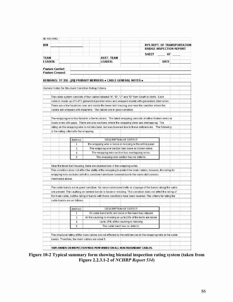
86

Figure 10-2 Typical summary form showing biennial inspection rating system (taken from

Figure 2.2.3.1-2 of NCHRP Report 534)

87

Figure 10-3 Typical form for biennial inspection showing detailed ratings (taken from


88

Figure 10-4 Typical form for biennial inspection of cable inside anchorage (taken from


89

Figure 10-5 Form for recording locations of internal cable inspections (taken from Figure

2.2.1.2.4-1 of NCHRP Report 534)

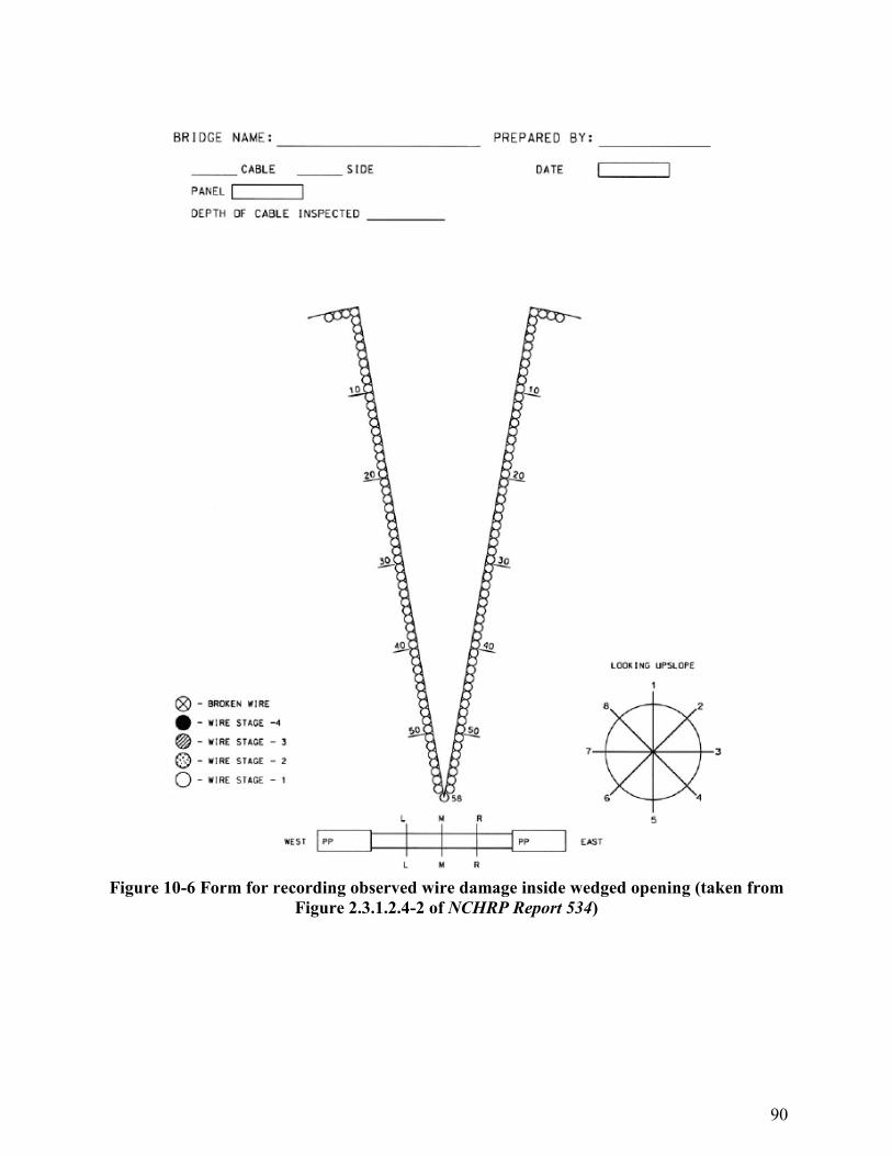
90

Figure 10-6 Form for recording observed wire damage inside wedged opening (taken from

Figure 2.3.1.2.4-2 of NCHRP Report 534)

91

Figure 10-7 Form for recording locations of broke wires and samples for testing (taken

from Figure 2.3.1.2.4-3 of NCHRP Report 534)

92

Figure 10-8 Form for recording cable circumference (taken from Figure 2.4.1-1 of NCHRP

Report 534)

93

10.2 STRENGTH EVALUATION FORMS Tables used for summaries and calculations associated with the Strength Evaluation example shown in Appendix A are shown in this section. The tables are presented so that the reader can use them or develop similar tables for a strength evaluation.

Table 10-1 Typical table that can be used for assignment of corrosion stages to individual rings of wires

94

Table 10-2 Typical table that can be used for assignment of corrosion stages to half sectors

of cable

95

Table 10-3 Typical table that can be used to record tension test results for a single wire

96

Table 10-4 Typical table that can be used to summarize the tension test results

97

Table 10-5 Typical table that can be used to summarize the number of broken and cracked wires

Table 10-6 Typical table that can be used for calculating the mean tensile strength

98

11.0 APPENDIX E: BTC METHOD FOR EVALUATION OF REMAINING STRENGTH AND SERVICE LIFE OF BRIDGE CABLES2

11.1 INTRODUCTION Given the importance of cable-supported bridges, random sampling and reliability-based analytical techniques are required for the assessment of remaining cable strength. State-of-the-art assessment techniques employ reliability criteria (similar to LRFD criteria), in which strength, strain and loads are known as probabilistic quantities. If an evaluation is conducted using these criteria, the results can be used to establish the tempo of bridge cable inspection and further evaluations in the future. Once probability distributions for wire mechanical properties, such as strength and strain, and loads are established, it’s possible to develop a cable failure mechanism and assess the serviceability of the cable. Use of probabilistic analysis in this approach is similar to the LRFD probabilistic analysis employed in the current AASHTO standards. Conventional cable strength evaluation methods rely heavily on the visual assessment of surface corrosion observed on individual wire surface. Wire sampling and strength evaluation, employed in these conventional methods, are dependent on visual condition of wires. This Appendix presents the BTC method, a probability-based, and U.S. patented [E.1]3 methodology for the evaluation of remaining strength and service life of both; parallel wire and helical wire bridge cables. The method applies to both zinc-coated and bright bridge wire. The method includes random sampling of individual cable wires from each investigated panel, mechanically testing the sampled wires, determining the probability of broken and cracked wires, evaluating the ultimate strength of cracked wires using fracture toughness criteria and utilizing the above data to assess the remaining strength of the cable in each panel. The probabilistic-based method assesses remaining service life of the cable by determining the rate of change of broken and cracked wires detected over a time frame, measuring the rate of change in effective fracture toughness over same time frame, and applying the rates of change to a time-dependent strength degradation prediction model. The BTC method provides sensitivity analysis to identify the key inputs which influence the estimated cable strength and assist the bridge owner in the decision making process. As such, the BTC method provides the bridge owner a greater understanding of the deterioration mechanisms at work in the cables as well as a comprehensive methodology that results in a higher level of confidence in the estimated strength and assessed remaining life of the bridge cable. The BTC method has been peer-reviewed by MTA Bridges & Tunnels, New York State Bridge Authority and New York State Department of Transportation. To date, the BTC method has been applied to assess remaining strength and residual life of the main suspension cables at the Bronx-Whitestone Bridge in New York City, and the Mid-Hudson Bridge, in Poughkeepsie, in the state of New York, USA.

2 Appendix E is authored solely by Khaled M. Mahmoud, Ph.D., P.E., Bridge Technology Consulting, New York City, email: [email protected]. Persons interested in using the BTC Method should contact the author of this Appendix. The inclusion of Appendix E does not necessarily constitute an endorsement of the BTC Method by the FHWA or the authors of this Primer. 3 Numbers in brackets refer to References provided at the end of this Appendix.

99

This Appendix provides a brief description of the BTC method for evaluation of remaining strength and residual life of bridge cables. 11.2 MAIN CABLE INSPECTION AND SAMPLING Internal inspection of main cables is recommended at a number of panels on each cable, depending on length of main cable, and known condition from history of previous cable investigations. For cables that never received internal inspections, a four to six panels are to be wedged, internally inspected and sampled from on each main cable. Prior to field inspection, a random sampling plan is prepared to extract wires for testing from each investigated panel. 11.2.1 Panel Selection Criterion The main goal of in-depth cable inspection is to assess the damage in the most deteriorated panels. Assessment of the structural integrity of the cable is achieved by calculating the factor of safety for each of the investigated panels. The panel with the lowest factor of safety will govern the factor of safety for the entire cable. Thus, our objective is to choose the most at-risk panels, and not random panels to calculate the safety factor for the cable. To that end, a study is conducted of the recorded history of external and internal cable inspections, wire breaks, and wire tests along the cable length to identify the most at-risk panels. Based on this history, a selection is made of the panels to be opened for internal inspection and sampling of wires. For main cables that have no previous history of internal inspection and show no evident external signs of deterioration, panels are randomly selected. 11.2.2 Random Sampling and Sample Size Determination Because it is unfeasible to sample and test every wire in the cable, only a sample of wires is removed for testing in the laboratory. In this way, sampling is done to generate a small group of wires that is as similar to the entire population of wires as possible. With that in mind, two questions arise; how well does the sample represent the larger population from which it was drawn? How closely do the features of the sample resemble those of the larger population? To answer these questions; a definition of sampling methods is introduced first. Sampling methods are classified as either probability or nonprobability. In probability samples, each member of the population has a known non-zero probability of being selected. Probability methods include random sampling, systematic sampling, and stratified sampling. In nonprobability sampling, members are selected from the population in some nonrandom manner. These include convenience sampling, judgment sampling, quota sampling, and snowball sampling. The advantage of probability sampling is that sampling error can be calculated. Sampling error is the degree to which a sample might differ from the population. When inferring to the population, results are reported plus or minus the sampling error. In nonprobability sampling, the degree to which samples might statistically differ from the population remains unknown. Thus random sampling presents the best representation and resemblance of wire condition throughout the entire bridge cable.

100

11.2.2.1 Random Sampling and Practical Considerations In random sampling, each wire in the available pool of wire samples has an equal and known chance of being selected. Random sampling procedures do not guarantee that the sample is representative, but they do increase the probability that the randomly selected wires will be representative of cable condition. There is a sampling error in the estimated cable strength because not every wire is sampled and tested. The sampling error describes the range that the estimated cable strength is likely to fall within. Sampling should be limited to provide an acceptable level of error in the estimated cable strength. This is to minimize vulnerabilities introduced in the cable cross section due to the sampling and removal of wires. A given cable investigation is not the last opportunity that wire samples will be removed from cable. Therefore, the following practical considerations must be recognized:

• It is not feasible to remove wires too deep in the wedge opening due to clearance problems in the wedge opening when cutting, splicing and re-tightening the splice.

• Even if a deeper wire is pulled with the use of a special tool out of the wedge, access for splicing and re-tightening would be very limited and damage to zinc coating of neighboring wires would become more likely.

• It is therefore our recommendation to minimize damage to main cable and not to remove samples from areas where they could not effectively be replaced and spliced.

• Outer wires are easily accessible, however, inner wires are difficult to reach for the purpose of tightening ferrules, and often a wire would be spliced with zero or small stress. This is evident by the slack condition of many spliced wires observed on suspension bridge cables.

In the random sampling plan, we define the sampling frame as the accessible group of wires that samples will be randomly selected from. Sampled wires constitute the sample size from which valid conclusions about the entire cable are based. This statistical inference is done with the aim of inferring the degraded condition of all wires from those found in the observed sample. By virtue of random selection of sampled wires, different conditions of wires would be included in the sample. 11.2.2.2 Sampling Size Determination It is important to evaluate the effect the sample size has on the error in the estimated cable strength. The error results from imprecision associated with estimating nominal cable strength based on a limited number of wire samples. Therefore an acceptable target level of error is set for the estimated cable strength. According to Article 3.4 of NCHRP Web Document 28 [E.2], the minimum expected finite fatigue life is taken as the fatigue resistance two standard deviations below the mean fatigue resistance. This is equivalent to a 97.73% one-sided confidence level. For the purpose of determining the sample size, we assume that the cable strength is determined only by the ultimate strength. The ultimate strength data, from previous investigations, if it exists, is fitted to an appropriate probability distribution. The sample size is then determined

101

based on a correlation between the strength distribution parameters and different level of error at a given level of confidence. In the case where no previous history of testing exists, sample size determination could be guided by random sample size established at other bridges by the BTC method. 11.2.2.3 Wedge Pattern Per the BTC method, the wedge pattern could be selected randomly. The eight-wedge pattern, which is shown in Figure 11-1 for illustrative purposes, is typically used for internal inspection of main suspension cables.

Figure 11-1 Eight-wedge pattern and pool of wire samples in the cable cross section

11.2.2.4 Sampling Frame of Random Sample The sampling frame, which is the pool of wire samples, should be limited to the group of wires that can be accessed for cutting, and splicing back to service load. This sampling frame depends on the diameter of the cable and length of panel opening, where larger diameter cables and longer panel opening provide more space for splicing sampled wires deeper in the wedge opening. For demonstration purposes, Figure 11-1 shows sampling frame, for a cable with 16-inch diameter and 6,080 wires. The first ten (10) rings of wires define the sampling frame; i.e. to a depth of approximately 2-inches which totals 160 wires. Those 160 wires are deemed easily

102

accessible for cutting, splicing and retightening back to service load. During the course of inspection, each wire that is randomly selected is assigned an I.D. number. Figure 11-2 shows a tagged wire with I.D. that reads PP 3-4S, W7/8, R4. This identifies a wire sampled from P.P. 3-4, in Wedge #7, Wedge #8 side, Ring # 4.

Figure 11-2 Photo showing the sample tag in wedge #7, wedge #8 side, ring #4, panel point

3-4 11.2.3 Inspection Procedures An access platform is typically constructed along the full length of each of the panels subject to internal inspection. After the removal of the Gauge 9 wrapping wire in each panel, the cable is typically wedged along four planes with an eight wedge pattern as shown in Figure 11-1, numbered in sectors from 1 to 8. The cable is wedged by the Contractor, utilizing plastic wedges driven to the center of the cable, as shown in Figure 11-3. As the photo shows, a stack of wedges was driven to allow for proper inspection and access to splice sampled and broken wires. The BTC method identifies proportion of broken wires based on wires found broken during inspection in each panel. The proportion of broken wires is treated as a probabilistic quantity. Figure 11-3 shows an interior broken wire that extended out of wedge opening following the driving of wedges. Broken wires are spliced to sustain service load if they are accessible for splicing.

103

Figure 11-3 Photo showing wedges driven to the center of the cable, interior broken wire is

shown Inspectors determine the visual condition of corrosion stages based on visual assessment of corrosion condition of the wire surface into four stages of corrosion that were first introduced by Hopwood and Havens in 1984 [E.3], [E.4], [E.5]. The evaluation of remaining strength per the BTC method is independent of the visual evaluation of stages of corrosion. However the four stages of corrosion are defined, as follows, for illustration of the inspection procedure, see Figure 11-4. Stage 1: the zinc coating of wires is oxidized to form zinc hydroxide, known as “white rust”. Stage 2: the wire surface is completely covered by white rust. Stage 3: appearance of a small amount of (20-30% of wire surface area) of ferrous corrosion due

to broken zinc coating. Stage 4: the wire surface is completely covered with ferrous corrosion.

104

Figure 11-4 Photographs showing the four stages of corrosion

11.3 WIRE TESTING PROGRAM Per the BTC method, the following tests are performed on the sample of wires collected from the bridge cable during internal inspection. Standard (18 inch) and long (60 inch to 72 inch) wire specimens are taken from each wire sample for testing. 11.3.1 Enhanced Tensile Strength Test in Standard Wire Specimens Each standard (18-inch) specimen is subject to enhanced tension test in which the full range of the stress strain curve is recorded. Mechanical properties of wires are measured by conducting tensile tests. A gage LVDT type extensometer is used for measurement of strain; to record true strain up to failure. Full stress strain curve for each specimen is provided with the measured ultimate strength, ultimate elongation, as measured along a gage length, Young’s Modulus, and yield strength. These properties of standard specimens are used for the evaluation of remaining cable strength. Fracture surfaces of all tested wire specimens are examined for presence of preexisting cracks. 11.3.2 Tensile Strength Test on Long Wire Specimens Each long (60-inch to 72-inch) specimen is subject to tension test, where length of the long specimen is determined based on maximum available distance between grips of the testing machine. The purpose of testing long specimens is to improve our ability in detection of preexisting cracks in wire test specimens. The probability of finding cracks in long specimens is higher than that of locating cracks in standard specimens. The reason for that is that in standard specimens, only about 12-inch of the specimen length is outside the grips of the testing machine. Therefore cracks might be missed if the tension test is limited only to standard specimens. For each long specimen, the measured ultimate strength, crack location and depth are provided. 11.3.3 Fracture Toughness Test Fracture toughness tests are performed on a group of wires from different panels for evaluation of fracture toughness of high strength cable wire [E.1]. The results of fracture toughness test are utilized in the assessment of remaining cable strength and residual life of the cable.

105

11.3.4 Fractographic and Scanning Electron Microscope (SEM) Evaluation Following the enhanced tension test on standard specimens, and tension test on long specimens, the entire set of fracture surfaces is subject to microscopic examination to identify preexisting cracks. The fractures are photographed at different magnifications (e.g., 20X, 100X, and 600X) to show the morphology of fracture surface, and crack depth for each cracked specimen. It is important to emphasize that the full stress strain curve for each cracked specimen shall be provided by the testing laboratory with the measured ultimate strength, ultimate elongation, as measured along a gage length, Young’s Modulus, and yield strength, and fracture strength for each test specimen. Measured crack depth and measured fracture toughness are used to establish the average ultimate strength of cracked wire proportion, as shown later. Scanning electron microscope (SEM) evaluation is provided for select test specimens with different crack depths to illustrate mode of crack propagation and morphology of fracture surface. 11.4 CABLE STRENGTH EVALUATION In the BTC method, the cable is represented as a series of parallel wires. The wire fails when the weakest segment fails. Therefore, the wire is as strong as its weakest segment. In ASTM standard tension test, the wire demonstrates almost perfect elastic behavior until plastification occurs at a randomly located weakest section. Incremental increase in strain usually leads to strain hardening in the weakest section, allowing for further load increase associated with deformation concentration until ultimate strength is reached. This behavior displays elastic-plastic behavior of steel, where the specific characteristics depend on the manufacturing process of the wire. 11.4.1 BTC Method Inputs The stress strain curves of wire specimens tested in the lab display a linear relationship between stress and strain up to the yield point and a nonlinear behavior between the yield and the ultimate point. This behavior is described by the Ramberg-Osgood relationship as follows:

n

ee α

Eσε

σσ

ε+= (11-1)

where σ, ε, E, are the stress, strain, and Young’s modulus respectively, n is the strain hardening exponents, εe, is the yield strain, σe is the yield strength and α is a fitting parameter. The test data provides measurements for yield strain, εo, Young’s Modulus, E, ultimate strength, σu, and ultimate strain, εu. Numerous test data of deteriorated wires show a larger scatter in the ultimate strain, compared with that of the ultimate strength, where coefficient of variation for ultimate strain is multiples of the coefficient of variation for ultimate strength. The coefficient of variation, for a given variable, is obtained by dividing its standard deviation by its mean value.

106

The noted significant variation in the ultimate strain illustrates the importance of including ultimate strain along with ultimate strength data in evaluation of remaining cable strength. The BTC method uses, as input, the four variables yield strain, εo, Young’s Modulus, E, ultimate strength, σu, and ultimate strain, εu, where each variable is described by an appropriate probability distribution, and the cable strength is estimated separately for each investigated panel. In each panel, the inputs include proportions of broken and cracked wires, which are treated as probabilistic quantities. The fracture toughness along with crack depth information are used to determine the average ultimate strength of cracked wires, σult cr., as follows:

c

ccr.ult

a πDaY

Kσ

= (11-2)

where Kc is the effective fracture toughness, ac is the critical crack depth and

DaY is the crack

geometry factor. 11.4.2 Choice of Probability Distributions According to the Engineering Statistics Handbook [E.6], life distribution models are chosen for one or more of the following three reasons:

• There is a physical/statistical argument that theoretically matches a failure mechanism to a life distribution model

• A particular model has previously been used successfully for the same or a similar failure mechanism

• A convenient model provides a good empirical fit to all the failure data. Whatever method is used to choose a model, the model should "make sense". Distribution models such as the lognormal and the Weibull are so flexible that it is not uncommon for both to fit a small set of failure data. Since data for these four variables is used to infer the estimated cable strength, it is important to "test" whether the distributions chosen are consistent with the collected data. For goodness of fit, different statistical tests are used; such as Anderson-Darling, Chi-Square, or Kolmogorov-Smirnov, to decide whether a distribution model under examination is acceptable. 11.4.3 Elongation Threshold Criterion, Mthreshold The ultimate elongation of wire is utilized in the BTC method to classify wires into two groups. Wires that fail at an ultimate elongation lower than a specific threshold elongation, Mthreshold, are categorized under the worst-wire proportion. All other wires, i.e., wires that demonstrate higher elongation than the threshold elongation, Mthreshold are classified as the better-wire proportion. By the above definition, the worst-wire proportion contains all cracked and broken wires, as well as some intact wires, while the better-wire proportion contains only intact wires.

107

To establish a threshold elongation, Mthreshold, such that we are confident that a cracked wire would fall within the worst-wire proportion, a one-tailed t-distribution at a given level of confidence, Mthreshold is used as follows:

Mthreshold = µ + (tα σ) (11-3) where µ and σ are, respectively, the mean and standard deviation of ultimate elongation of the set of cracked wire specimens, while tα is obtained from t-distribution tables at a given level of confidence. In the following section, condition of any wire is determined as broken, cracked, or intact. 11.4.4 Determination of Wire Condition The possible outcome of the condition of the wire as broken, cracked or intact is treated as a discrete random variable, X, such that:

P(X = xj) = Pj; j = 0,1,2; ∑ ==

2

0jj 1p (11-4)

where, x0, x1, and x2 represent in this case broken, cracked and intact wire respectively. The probability of realizing a broken wire is defined as p0, while p1 is the probability of realizing a cracked wire, and p2 = 1 - p0 – p2 is the probability of having an intact wire. The probability of broken wires, p0, in each panel is determined based on the number of wires found broken during inspection. On the other hand, the probability of cracked wires, p1, is determined from assessing the ratio of cracked samples, based on the fractographic evaluation of the fracture surfaces of all wires tested in tension. For determination of the probabilities of broken and cracked wires, p0, and p1, in the investigated panel, the effect of broken and cracked wires in the adjacent panels is considered. When a wire is cracked or fractured in a given panel, it redevelops its load carrying capacity after a certain length, known as the redevelopment or recovery length. While a wire that contains a crack does not lose its entire capacity to carry load, part of its load carrying capacity is lost due to the presence of the crack. The recovery length concept is applied to cracked wires, whereas a cracked wire in a given investigated panel would regain its full load carrying capacity at the end of the recovery length. The following section introduces a discussion on the recovery length and assumption made in this appendix. 11.4.5 Wire Recovery Length When a cable wire under tension breaks, or cracks, at one location there is sufficient friction within the cable that at some distance from the location of break, or crack, the wire sustains the same tension as if it were unbroken or uncracked. The frictional forces develop due to the radial pressure applied by the taut wrapping wires and cable bands. Additional pressure and friction are

108

generated near the location of break or crack in wire due to the Poisson’s effect. Because the cable is restrained from lateral expansion by the radial pressure provided by the wrapping wire and cable bands, the Poisson’s effect increases the inter-wire contact forces. One can postulate a length over which all these frictional forces cumulatively equal the full tensile strength of the wire which had broken or cracked. This length is defined as the clamp or recovery length. Results of analysis by contact-stress theory showed that the recovery length for an 18” diameter cable with 7,697 parallel wires is 5ft [E.7]. The conclusions of the study demonstrate the effectiveness of wrapping wire and cable bands in redeveloping the strength of a defective wire. It is important, however, to consider the effect of slippage of the wrapping wire or cable bands on the recovery length. Slippage in the cable band may occur due to loss of tension in cable band bolts. This would subsequently reduce the restored load carrying capacity of a broken or cracked wire, at the slipping band. This problem has been encountered on many suspension bridges. In 2009, failure of nine heavy-duty nuts of cable band bolts on a major suspension bridge has been reported. All the cable band nuts and bolts were replaced in the late 1990s as part of a project to replace the suspender ropes. An investigation into the failure of the nuts has identified a number of design and specification decisions and construction methods that may have contributed to the cracking, including replacement of the original bolts with metric versions with a thinner section than the originals. The nuts are small compared with similar ones on other suspension bridges. Another factor was the use of a higher grade of steel, which meant that the nuts are less ductile, i.e., more brittle, than the originals. Misalignment of washers may have led to uneven loading in the nuts. In addition, the protective coating was inadequate and allowed moisture to cause damage. To account for possible slippage of unwrapped external wires and cable bands, and considering gaps of broken wires that were measured during different cable investigations, a broken or cracked wire is assumed to redevelop its full load carrying capacity after two consecutive panel lengths, at each end of the investigated panel. Therefore the effective number of broken or cracked wires in a panel under evaluation includes wires that are broken or cracked in the investigated panel in addition to the number of broken or cracked wires that are not developed in two flanking panels at each side of the investigated panel. 11.4.6 Broken Wires The number of broken wires in the exterior ring of the cable in each panel is those identified broken upon the removal of the wrapping wire prior to the wedging operations. Interior broken wires are those uncovered during the wedging operations. As explained earlier, the interior broken wires are typically determined in an eight-wedge pattern, in each panel. 11.4.6.1 Exterior Broken Wires Wires found broken along the exterior ring of the cable are readily recovered upon the removal of the wrapping wire in each panel.

109

11.4.6.2 Interior Broken Wires The total number of inspected interior wires represents a small fraction (≈ 10%) of the wires in the cable cross-section. Therefore in the following analysis, the probability of broken wires, p0, is assessed based on the observed interior broken wires, in each panel. The proportion of broken wires, p0, in each investigated panel, is determined by dividing the number of interior broken wires divided by the number of inspected wires. 11.4.7 Cracked Wires The probability of cracked wires, p1, in each panel, is determined by dividing the number of cracked wires by the number of tested wires sampled from each panel. As mentioned earlier, cracked wires are identified by microscopic examination of all the wires sampled and tested in each panel. 11.4.8 Strength Evaluation using the BTC Method In the evaluation of the cable strength in each panel, per the BTC method, the input data consists of the following:

• Probability distributions and correlation for test data for intact wires, [εe, E, εu, σu]Intact • Probability distributions and correlation for cracked wires, [εe, E, εu, σu]Cracked • Probability of broken wires, p0 • Probability of cracked wires, p1

Using the above input data, the stress strain curve for each wire is constructed. All the wires in the cable cross-section subjected to the same strain. The strain is applied in increments, and the wire fails when it reaches its ultimate strain. Failed wires are discounted from the strength calculations. This process is repeated for the entire set of wires until all the wires reach their ultimate elongation. The load carrying capacity for the cable reaches zero at maximum elongation. The estimated cable strength is the maximum load calculated. 11.5 BTC METHOD FORECAST OF CABLE LIFE Main cable wires degrade and suffer reduction in load carrying capacity over time. The BTC method forecasts cable degradation as a function of wire mechanical properties, and time. As explained earlier, the cable cross-section is divided into three groups, namely intact, cracked and broken wires. The broken wires group has no load carrying capacity in the investigated panel. To establish rate of degradation, it is necessary to estimate the time for onset of degradation for both intact and cracked wires, time at which degradation is triggered, and proportions of cracked and broken wires. This is achieved based on data collected under current and previous investigations.

110

11.5.1 Forecast of Degradation in Intact Wire Strength Degradation of the strength of intact wires is estimated, based on wire test history, however limited, at different points in time, using the following model:

)t,t,(fFF

211

2 κ= (11-5)

where F1 and F2 are the breaking loads corresponding to the two breaking times t1 and t2, and κ is a degradation kinetic that depends on environment, strength and time. 11.5.2 Forecast of Degradation in Cracked Wire Strength Continuous loading on the cable leads to crack growth in the cracked wires, leading to fracture when the crack depth is such that the stress intensity factor is equal to its critical value, known as the fracture toughness. Due to environmental degradation, the effective fracture toughness is reduced resulting in reduced strength of cracked wires. The environmental degradation is manifested in the appreciable reduction of the strain energy density, W0, and effective fracture toughness, as first introduced for bridge cable wire in Reference E.8. Therefore fracture toughness and strain energy density measurements provide important information regarding the strength degradation of cracked wires. The strength of the cracked wires at time t2 is assessed based on the measured effective fracture toughness at time t2. The strength of the cracked wire proportion at time t2, 2tcr.ult )σ( is then given by:

c

tctcr.ult

a πDaY

)K()σ( 2

2

= (11-6)

where

2tc )K( is the effective fracture toughness at time t2, ac is the critical crack depth and

DaY is the crack geometry factor.

The estimate for effective fracture toughness of degraded wire, at time t2, is a function of the strain energy density, which in turn, is evaluated from the stress-strain curve [E.8]. A relationship between the fracture toughness and the strain energy density for a bridge wire was first introduced by the BTC method, as follows:

02c WβK = (11-7)

where β is a function of the elastic properties of the material. The effective fracture toughness,

2tc )K( , at time t2, is estimated from:

111

))W(,)W(,)K((f)K(2112 t0t0tctc = (11-8)

where

2t0 )W( is the corresponding strain energy density at time t2, while 1t0 )W( and

1tc )K( are, respectively, the strain energy density and effective fracture toughness of the wire material at time t1. Forecast of degraded strengths for intact and cracked wires, as well as updated proportions of broken and cracked wires at different points in time are utilized to build a cable strength degradation curve and estimate the remaining service life of the cable. 11.6 SENSITIVITY ANALYSIS The input values and assumptions of probabilistic models are subject to uncertainty. This section presents sensitivity analysis for the estimated cable strength due to uncertainty in the inputs. The purpose of sensitivity analysis is to:

(i) identify the key inputs which influence the estimated cable strength. (ii) assess whether the estimated cable strength and the decision making process are

likely to be affected by such uncertainties. To conduct sensitivity analysis, key inputs are identified. The values for those inputs are changed above and below a specific base value for the cable strength. The effect of each input is changed at a time, while the other inputs are kept at values corresponding to the base value, and the cable strength corresponding to changed input is then assessed. This process is repeated for the different inputs, above and below the base values, and the effect of uncertainty in each input is quantified. Conclusions are then made about the ranking of sensitivity of cable strength to uncertainties in different inputs. The following section identifies the key inputs subject to sensitivity analysis. 11.6.1 Key Inputs The following inputs are identified as influential in the evaluation of the remaining cable strength:

• Effect of adjacent panels • Proportion of cracked wires • Ultimate strength of cracked wires • Proportion of broken wires

As demonstrated earlier in this Appendix, the proportion of broken wires is estimated from field inspection findings of broken wires. The proportion of cracked wires is evaluated based on the presence of preexisting cracks in tested wires. From the analysis of inspection and testing results, it is evident that both proportions demonstrate a range of variation and it is important to define the range over which the sensitivity analysis is performed. The ultimate strength of cracked wires is an input that varies depending on the effective fracture toughness at a given point in time. The effect of these inputs on the estimated cable strength is studied by varying the value of inputs above and below a base value.

112

The base value for this sensitivity analysis is the expected value of cable strength in the investigated panel, which is assessed based on the effect of two adjacent panels at each end, with proportion of broken wires, p0, and proportion of wire cracking, p1. To study the effect of proportion of cracked wires, p1, a proportion value ∆ is added to p1, while all other inputs are kept at the base value. The following set of inputs will be used to assess corresponding cable strength:

• Number of adjacent panels: 2 panels • Proportion of broken wires: p0 • Proportion of cracked wires: (p1+ ∆) • Ultimate strength of cracked wires: (σult cr.)

The cable strength is estimated based on the above set of inputs. Then, the cable strength is estimated once more, but with proportion ∆ being subtracted from the proportion of cracked wires, while again the other inputs are kept at their base values, as follows:

• Number of adjacent panels: 2 panels • Proportion of broken wires: p0 • Proportion of cracked wires: (p1- ∆) • Ultimate strength of cracked wires: (σult cr.)

The same process is repeated for all other inputs using the same ∆, above and below the base values. The reason for choosing the same value of proportioning, ∆, is to ensure the validity of conclusions drawn regarding relative sensitivity of assessed cable strengths to uncertainties in different inputs. 11.6.2 Sensitivity Indices The BTC method defines a sensitivity index as a number which gives information about the relative sensitivity of the estimated cable strength to different inputs of the model. The sensitivity index (SI) is given by Hoffman and Gardner [E.9]:

SI = (Dmax - Dmin) (11-9) where Dmax is the output result when the input in question is set at its maximum value and Dmin is the result for the minimum input value. The calculated sensitivity indices provide ranking for the analyzed inputs. This ranking provides the bridge owner with a clear picture of how the different inputs affect the estimated cable strength by calculating the range of variation in the cable strength corresponding to the range of variation for each input. 11.7 APPENDIX E REFERENCES

E.1. Mahmoud, K. (2009). “Method for Assessment of Cable Strength and Residual Life,” United States Patent 7,992,449, August 2, 2009.

113

E.2. Lichtenstein Consulting Engineers, Inc. (2001). NCHRP Web Document 28: Manual

for Condition Evaluation and Load Rating of Highway Bridges Using Load and Resistance Factor Philosophy, NCHRP Project C12-46.

E.3. Hopwood, T. and Havens, J.H., (1984a). Corrosion of Cable Suspension Bridges,

Kentucky Transportation Research Program, University of Kentucky Lexington, Kentucky.

E.4. Hopwood, T. and Havens, J.H, (1984b). Introduction to Cable Suspension Bridges,

Kentucky Transportation Research Program, University of Kentucky, Lexington, Kentucky.

E.5. Hopwood, T. and Havens, J.H, (1984c). Inspection Prevention, and Remedy of

Suspension Bridge Cable Corrosion Problems, Kentucky Transportation Research Program, University of Kentucky, Lexington, Kentucky.

E.6. NIST, (2003). Engineering Statistics Handbook, U.S. Commerce Department's

Technology Administration. E.7. Raoof, M. and Huang, Y.P. (1992). Wire Recovery Length in Suspension Bridge

Cable, ASCE Journal of Structural Engineering, Vol. 118, N0. 12, December, 1992, 3255-3267.

E.8. Mahmoud, K.M. (2003). Degradation of Bridge Cable Wire Due to Stress Corrosion

Cracking and Hydrogen Embrittlement, International Mesomechanics Conference, University of Tokyo, Japan.

E.9. Hoffman, F.O. and Gardner, R.H. (1983). Evaluation of uncertainties in environmental

radiological assessment models, Radiological Assessments: A Textbook on Environmental Dose Assessment, J.E. Till and H.R. Meyer (editors). US Nuclear Regulatory Commission, Washington D.C., Report no. NUREG/CR-3332, pp. 11.1-11.55.

http://www.doc.gov/