Embed Size (px)
Citation preview

TRANSACTIONS OF SOCIETY OF ACTUARIES 1990 VOL. 42
PRICING AND UNDERWRITING GROUP DISABILITY INCOME COVERAGES
ROY GOLDMAN
ABSTRACT
This paper summarizes the salient techniques for evaluating and pricing the risks in group disability income coverages. Ideas and methods are pulled together from published sources and practical experience. The theory is illustrated by realistic examples and applications.
The risks in both short-term and long-term products are discussed from the vantage points of underwriting, marketing, and administration. The con- cept of manual rates is explained, and sources of information are given. Illustrative manual rates are developed by using sources published by the Society of Actuaries.
The paper contains examples of how to evaluate long-term-disability (L'I"D) experience for quoting on new business or for rerating or analyzing business in force. Methods of calculating the variance (that is, risk) in expected LTD experience are presented, and practical applications are given. The paper concludes with a succinct discussion of both classical and Bayesian credi- bility. The theory is then applied to a realistic block of business to obtain credibility factors for experience-rating calculations.
I. INTRODUCTION
In this paper we discuss pricing techniques for group disability income coverages. We cover the pricing of both short-term- (STD) and long-term- disability (LTD) products for large and small groups. We also address un- derwriting, marketing, and administrative issues because these must be con- sidered when pricing these or any other group products.
The paper begins with a description of the risks to be underwritten and priced. We then discuss the development of manual rates and the adjustment of these rates for particular benefit designs and covered groups. The next section is devoted to the evaluation of LTD experience for proposal and renewal quotes on larger groups. Included is a presentation on credibility theory and the calculation of variance of expected benefits. In the final section we discuss the establishment of LTD claim reserves for both statutory and tax purposes in the U.S. and Canada.
171

172 GROUP DISABILITY INCOME COVERAGF.S
II. DESCRIPTION OF DISABILITY INCOME COVERAGES
A. Short-Term-Disability Income (STD)
Most employee benefit programs provide coverage to replace income lost while the employee is disabled for a short term. Benefits may be provided under a variety of plans: Social Security Disability Income (SSDI), Canada/ Quebec Pension Plans, workers' compensation plans, temporary disability benefit plans (in five states and Puerto Rico), wage loss replacement plans (Canada Unemployment Insurance Act), sick-leave plans, union and asso- ciation plans, individual insurance plans, pension plans, group life insurance plans, group LTD plans, or group STD plans. Group STD plans are often self-insured by employers with more than 200 employees because costs can be predicted fairly accurately for groups of this size. In the U.S., 50--60 million persons have short-term-disability income protection through their employers, unions, or associations on an insured or noninsured basis [21], Table 1.5].
1. Benefit Design STD may be referred to as "accident and sickness, . . . . group weekly
indemnity," or other names. Typically, these plans provide a percentage of an employee's weekly income when the employee is unable to perform his or her occupation because of a nonoccupational accident or sickness. Usu- ally, under self-insured plans, salary is continued at 100 percent by the employer for a short period and then reduced to between 50 percent and 66-2/3 percent (between 50 percent and 75 percent is typical for the Canadian market) for the remainder of the period. Insured plans pay only at the reduced level. The maximum benefit duration is generally 13, 26, or 52 weeks and can vary by length of service. Benefits begin after a waiting (elimination) period of 0 to 14 days. Usually the elimination period is zero for accidents and seven days for sickness. Such a plan with a 26-week maximum benefit is known as a 1-8-26 plan, where the 1 and 8 refer to the day benefits begin for an accident and for a sickness. One variation is to shorten the elimination period to zero if the employee is hospitalized for a sickness (known as a 1-1-8-26 plan). Surveys by the Health Insurance As- sociation of America (HIAA) [14] present a picture of STD coverage issued in 1986; see Table 1. These data are based on 262 cases covering 25-499 employees.
GROUP DISABILITY INCOME COVERAGES
TABLE I
NEW PLA~S ISSUED 1N 1986
173
Commencement of Benefit Period
Day Benefits Begin
Accident
1 1 1 1 8
14 All Others
Sickness
1 4 8
14 8
14
Percentage of Employees
4.0% 2.4
73.9 3.1 6.4 7.3 2.9
Length of Benefit Period
Duratioa Percentage of (weeks) Employees
13 17.2% 26 75.2 52 6.8
104 0.8
Amount of Weekly Conlfibution Income Provided
Percentage of Ma~aum Percentage of Payor of Premiums Weekly Benefit Employees
Employer Employer and employee Employee
Employees
60% $70 30 70-109 10 110-149
150-199 200-299
>$300
Average Amount o~ Weekly Income Pmvidexl
Average Weekly Percentage of Benefit Employees
< $60 18.8% 60-109 19.7
110-159 24.1 160-199 11.8
>$200 25.6
11.0% 16.1 7.5
20.9 14.9 29.6
2. Underwriting Concerns
The nature of the STD risk is one of high frequency with relatively low maximum benefits. The underwriter needs to be concerned with the follow- ing case characteristics:
(1) Definition of EligibiliO~ and DisabiliO,--clearly defines the risks that are meant to be covered, is easily administered.
(2) Amount of Benefits--not so high as to encourage greater frequency and malingering. (3) Benefit Duration and Elimination Period--coordinates with other benefit plans (for
example, sick leave and LTD), does not encourage absenteeism. (4) Nonduplication--with other employer plans and state or federal sickness or workers'
compensation plans. (5) Industry--Are the benefits predictable in the aggregate or can the employee or
employer select against the insurer by exercising control over utilization? Industries

174 GROUP DISABILITY INCOME COVERAGES
that need careful underwriting or are uninsurable have one of the characteristics: (a) High turnover of employees (b) Seasonal employment (c) Poor financial condition (d) Highly cyclical or prone to failure (e) Remote locations (f) High frequency of work-related disability (g) Self-employment.
following
(6) Employer Characteristics--ls the employer committed to the plan? Commitment is shown by the level of employer contributions, employee participation, and extent of employee benefits provided. Commitment to an insurance program is also mea- sured by the frequency in the change in insurance carrier. Another measure of potential antiselection by insureds is the degree of control a group policyholder exercises over the insureds, for example, a single employer versus a multiple em- ployer or an association of individuals.
(7) Other Coverages--In the U.S., STD is often quoted with either life insurance or other health coverages. The presence of other coverages reduces antiselection against the plan and lowers retention somewhat.
(8) Individual Underwr/t/ng--Medical underwriting (short-form health history with follow- up attending physician's statement) is generally required on small groups (fewer than 10-20 employees, depending upon the insurer) and for individuals with high amounts of coverage.
B. Long-Term-Disability Income (LTD)
Most salaried employees are covered for income lost while disabled over an extended period; however, coverage is less prevalent among workers in general in the U.S. The HIAA estimates that 18-19 million persons had group LTD coverage, insured and noninsured, in 1986 [21, Table 1.5].
Among employers and large-group insurers in the U.S., LTD coverage receives less attention than medical coverages because LTD costs only about $100 per year per employee, compared to $2500 for medical coverage. However, the risk in LTD is much greater because, although the frequency is low, the average claim cost is $40,000--50,000, and the variance in claim costs is large in relation to expected costs. As a result, all but the largest employers insure their LTD coverage. Insurers, on the other hand, must carefully underwrite the risk and pay special attention to claim administration to assure that:
(1) Only those eligible receive benefits (2) Benefits are paid only as long as the claimant remains disabled, as defined by the
plan

GROUP DISABILITY INCOME COVERAGES 175
(3) All benefit offsets are taken into account (4) The claimant is encouraged and rehabilitated to return to work as soon as possible.
1. Benefit Design LTD plans provide a percentage of an employee's monthly income when
"disabled." The maximum benefit duration is usually to age 65 (except for those disabled after age 60), and the most common elimination period is six months (26 weeks), although three months (13 weeks) is gaining in popu- larity and is most common in the western U.S. An employee normally qualifies for benefits when "totally disabled," which is defined to mean that:
(1) The claimant is under the regular care of a doctor, and (2) Due to sickness or accidental injury, the claimant is unable to perform, for wage
or profit, the material and substantial duties of his or her own occupation.
After a specified period, usually two years of benefits, condition (2), called OWN OCC, becomes more restrictive (called ANY OCC):
(3) The claimant is unable to perform, for wage or profit, the material and substantial duties of any occupation for which he or she is reasonably fitted by education, training, or experience.
Some plans covering only blue-collar workers or smaller groups may only provide benefits based on the ANY OCC definition because of the added risk associated with the OWN OCC definition. In some states, court deci- sions have made it difficult for insurers to impose the ANY OCC clause.
Benefits may also be paid for partial disabilities, but usually only after the claimant is "totally disabled." Rehabilitation is encouraged by providing coverage for rehabilitation counseling and training and by allowing a trial return to work while still paying 50-70 percent of usual monthly benefits. Plan benefits may be offset by benefits payable under any or all the plans listed in Section II.A except for individual policies. There is almost always an offset for disability benefits provided by SSDI or the Canada/Quebec Pension Plan.
According to surveys by the HIAA [14] and by Hewitt Associates [19], we have the picture of LTD coverage shown in Table 2. The HIAA data are from 130 cases covering between 25 and 499 and employees; the Hewitt survey covered 800 major employers. About 44 percent of the employees were covered for partial disabilities (if preceded by a period of total disa- bility), and 63 percent for rehabilitation services.

TABLE 2
NEW PI..A~S ISSUED Ir~ 1986 (HIAA)
Commencement of Benefit Period Length of Benefit Pcdod Elimination Percentage of Pcrcen~,ge of
Period Employees Maximum Duration Employ~s 0 2.1% 2 Years 3.1% 1 Month 13.2 5 Years 3.5 2 Months 2.2 To age 65 or 70 89.3 3 Months 38.8 Other 4.1 6 Months 35.2 All Others 8.5
Awmge Amount ¢~ Mooth}y It~me Pn3vided Average M~athly
Benefit <$5OO
500-599 6OO-699 700-799 80O-899
>$90O
Percentage of Employees
4.6% 11.9
2.8 4.7 2.2
73.8
I Percentage of Offsets Employees
All employer and governmental plans 18% Only governmental 16 Only Social Security [ 43 Other approaches [ 23
Percentage of Payor of Premiums Employees
Employer 73% Employer and employee 22 Employee 5
All ~lm~l Hans (Hewia) Percentage of Social Security Percentage of
Percentage of Pay Plans (1986) Offsets I Plans (1986) <6O% 6O% 65--67%
:'7O% Graduated formula Employee selection Other (for example,
pay- or service- related)
15% 53 12 2 I0 3 5
Fam~b' Primary No offset Other
48% 40 9 3
176

GROUP DISABILITY INCOME COVERAGES
TABLE 2--Continued
177
Percentage of plans with r ~ y Soc~ Secu~y Offset
Percentage of Pay (1984) < 60% 2%
60% 45 65--67% 60
>70% 80 Employee selection 50 Other 44
Maximum Monthly Percentage of P~ms Benefit (1986)
<$2500 $2501-3000
3001---4000 4001-5000
>5001 No dollar maximum Employee's option
5% 6
11 24 25 26
3
2. Underwriting Concerns
Because of the significant risk in LTD coverage, as measured by the ratio of the variance in benefits to expected benefits, careful underwriting by the field and home office staff is of paramount importance. The product should be designed and priced to fulfill the goals of the company's marketing strat- egy: large versus small groups, specific industry or occupational groups, and pooled versus nonpooled (that is, experience-rated) business. For ex- ample, small group coverage may compete with individual policies, thus necessitating coverage options such as cost-of-living increases and residual disability (that is, partial disability without requiring prior total disability). As another example, experience-rated business requires larger margins for retrospective dividends or refunds.
With respect to risk selection and benefit design, the objective is always to minimize antiselection and malingering. All the underwriting concerns listed for STD also apply to LTD. In addition, we should add the following case characteristics: (9) Occupation within Industry--Is the coverage for executives, salaried professionals,
or nonsalaried workers? (10) Nonmedical Maximum--Should individual underwriting be required for any of the
higher compensated employees? (11) Quality of Transfer-of-Business Information (TBI)--Most groups will have current
LTD coverage with another carder. Evaluation of prior experience is an important

178 GROUP DISABILITY INCOME COVERAGES
part of the rating process, regardless of whether LTD is quoted with other cov- erages, especially for cases with 500 or more employees. The TBI must be received with sufficient claim detail to be worthwhile. Ideal TBI includes age, sex, diag- nosis, date of disability, date of recovery, monthly benefit, monthly offsets, and current claim reserve on all claims incurred in the experience period. Rate, ex- posure, and paid claim information should also be included for each year in the experience period.
III. g a l . , RATES
In group insurance, "manual rates" refer to a company's standard rates for the range of coverages offered for all types of groups the company anticipates insuring. These rates are intended to cover the cost of anticipated benefits and expenses in addition to providing the required margin and profit. In general, manual rates reflect retention for groups of a specific size. For other sized groups, retention factors (see Section III.B.8) are applied to the manual rates to obtain "standard" or "payable" rates. Manual rates gen- erally serve four purposes:
(1) Satisfy state rate filings (when applicable). (2) Represent rates that would be charged in the absence of credible TBI; they are also
used as part of the weighted average in prospective experience rating evaluation where prior experience is given less than 100 percent credibility.
(3) Used to price benefit options or calculate cost relativities between two benefit designs (for example, comparing a 1-day accident, 8-day sickness STD plan to an 8-day accident and sickness plan).
(4) Used in retrospective experience analyses to put all plans of a certain type on a common footing (for example, in calculating company-wide expected loss ratios).
Usually many data sources are researched in order to develop manual rates. The best source is the company's own experience data. If such data are unavailable or insufficiently reliable or credible, frequently used alter- native sources are the experience studies compiled by committees of the Society of Actuaries and published in the Transactions, Transactions Reports of Mortality, Morbidity and Other Experience or other Society publications. Rate filings made by competitors are public information in many states, and these can be useful sources from which to build manual rates. Consulting firms can also be helpful. Often data for manual rates can be obtained only by performing basic research. This includes a literature search through gov- ernmental and industry publications and discussions with industry or other experts in the field. When sources outside the company are used, appropriate adjustments should be made to reflect anticipated differences in underwriting

GROUP DISABILITY INCOME COVERAGES 179
practices. Manual rate development sometimes becomes a good test of an actuary's creative ability and judgment.
A. Short-Term-Disability Income
An important source of data for STD manual rates is the Report of the Committee on Group Life and Health Insurance that appeared in the TSA Reports through 1983. There were 36 annual reports on the morbidity ex- perience under contracts for Group Weekly Indemnity insurance.
1. TSA 1982 Reports
The report in the TSA 1982 Reports [9] is typical of the format. This report contains the experience of employer/employee (non-union) groups for the years 1977-1981. Six large U.S. companies contributed data, the ma- jority of which contained exposures and claims based upon policy years ending in the designated calendar year. The TSA 1982 Reports marked the first time that the experience studied was limited to plans with full maternity benefits. The Pregnancy Discrimination Act of 1978, an amendment to Title VII of the Civil Rights Act of 1964, imposed the requirement on all groups of 15 or more lives that, in any benefit program, pregnancy-related disabil- ities must be treated the same as disabilities caused or contributed to by any other medical conditions.
Experience is shown as a ratio of actual claims to expected (or tabular) claims. Exposure is measured in units of $10 of weekly benefits in force. Tabular claims are calculated by multiplying the exposure for a given plan by the appropriate tabular claim cost. The tabular claim cost in this study is the annual claims per $10 weekly benefit for 1947-1949, as developed by Miller [13]. These tabular claim costs are shown in Table 3 along with the ratio of actual 1979-1981 combined policy years' experience to these tabular costs.
The major factors influencing STD experience are age, sex, elimination period, duration of benefits, industry, and size of group. The TSA 1982 Reports [9] provides insight on all these except age and industry. The tabular costs themselves show the relationship among sex, elimination period, and maximum benefit duration in 1947-1949. The actual-to-tabular (A/T) ratios in the report exhibit the change in these relationships 30 years later. Table 1 of [9] shows that the A/T ratio for 26-week plans is higher than that for 13-week plans, thus indicating a relative worsening of experience on plans of longer duration.
180 GROUP DISABILITY INCOME COVERAGES
TABLE 3
1947-1949 WEEKLY INDEMNrrY TABUI.~ A~UAL CLAIM Costs PER $I0 WEEKLY B~a~rr
Plan Male with Maternity without Maternity 1979-1981 to Tabular 13-Week Plans
l'--4-13 $5.77 $13.09 $9.67 1.02 6-4-13 5.69 12.91 9.49 1.96 1-8-13 4.99 11.40 7.98 1.04 g--8-13 4.81 11.01 7.59 0.70 l'otal 0.97
26-Week Plans l-4-26 7.32 14.56 11.14 1.25 I 4 26 7.23 14.37 10.95 1.30 l-8-26 6.50 12.81 9.39 1.13 ?,-8-26 6.31 12.41 8.99 0.83 l'otal 1.10 3rand Total 1.08
Other noteworthy findings include the following: (1) Nonmaternity experience under plans with maternity benefits is worse than the
maternity experience on these plans [9, Table 2]. (2) A/T experience tends to worsen as the size of the group increases for groups under
1000 lives [9, Table 4].
TABLE 4
Ratio of Case Size A~ual-m-Tabular
<50 lives 50-99
100-249 250-499 500-999
>1000 Total <1000 Grand Total
0.98 0.98 1.07 1.22 1.25 1.00 1.15 1.08
(3) In past reports, the ratios tended to increase as the female percentage increased for a group with between 11 and 70 percent female content. There was no general pattern in the TSA 1982 Reports. The results should be used with caution because they are based on relatively few claims and, hence, are not very cred~le [9, Table 5].

GROUP DISABILITY INCOME COVERAGES
TABLE 5
Female Ratio of Percentage Actual..to-TJbular
<11% 1 1 - 2 0 21-30 31--40 41-50 51..-60 61-70 71--80 81-90 91-100
Grand Total
0.95 0.85 0.76 1.00 0.92 0.82 1.25 0.87 1.00 0.92 0.92*
*Based on only 10,440 claims.
181
2. TSA 1980 Reports, TSA 1972 Reports, and Miller
The last report by the Society of Actuaries on experience by industry for Group Weekly Indemnity insurance appeared in the TSA 1980 Reports [7]. The A/l" ratios combine experience on plans with full maternity (at 40 per- cent of tabular) with experience on plans with no maternity, but they are still useful indicators of the differences among industry groups. A company could also use its data for medical insurance as a guide to setting industry factors.
The TSA 1972 Reports [6] compare Group Weekly Indemnity experience in the U.S. and Canada. There did not appear to be any significant differ- ences at that time, although A/I' ratios in Canada were generally higher than those in the U.S. for plans with no maternity benefits and lower for plans with maternity benefits.
No discussion of sources would be complete without mention of Miller's landmark paper "Group Weekly Indemnity Continuation Table Study" [13], which is the basis for the tabular claim costs used today. In addition to investigations by plan, sex, accident, and sickness, the paper includes a daily continuance table, study of seasonality, and experience by age. Only duration of disability is reflected in the age data. The average durations increase by age for both males and females.
3. Manual Rate Calculation-Example I
How would an actuary use the above sources to develop manual rates? For example, consider determining the manual rate for a 1-8-26 STD plan paying benefits (with full maternity) equal to 50 percent of weekly salary.

182 GROUP DISABILITY INCOME COVERAGES
Suppose manual rates are needed for a 100-life printing firm whose em- ployees are 70 percent male. Assume the insurer's retention for this size group is 18 percent of manual premium.
1. Tabular claim costs from Miller's table are 6.50 for males and 12.81 for females. 2. The A/T ratio is 1.13 for a 1-8-26 plan. 3. The A/T ratio for a 100-life plan is approximately 0.5(0.98 + 1.07) = 1.025. 4. The ratio of (3) to the aggregate A,rl" ratio is 1.025/1.08=0.95. 5. The A/T ratio for a plan with 30 percent female employees is approximately
0.5(0.76 + 1.00) = 0.88. 6. The ratio of (5) to the aggregate A/T ratio is 0.88/0.92=0.97. 7. From the TSA 1980 Reports [7], the ratio of the printing industry A/T to the aggregate
A/T is 0.82 for groups under 1000 lives. 8. By using (1), (2), (4), (6), and (7), we obtain expected annual claim costs per $10
weekly benefit: (1.13) (0.95) (0.97) (0.82) [(0.70) (6.50) + (0.30) (12.81)] = 7.17.
9. Manual rate = 7.17/(1-0.18) = 8.74.
In steps (3) and (5), an average factor was used because 30 percent female and 100 lives are boundary points in the A/T tables. This calculation also assumes there is no interaction among the factors. When this methodology is used, the final rates must be inspected for reasonableness because signif- icant A/T differences among plans can lead to anomalous results.
4. Individual Loss-of-Time Experience
The reports on individual loss-of-time experience, which are also pub- lished in the Reports [5], provide additional insight on the effects of age and industry. Experience for the first year of a benefit period is studied by age, sex, elimination period, accident, sickness, and occupation group. Occu- pation Group I consists of occupations that involve little exposure to an accident hazard and do not require heavy physical activity. Occupation Group II consists of occupations that involve a greater degree of exposure to ac- cident hazards or whose jobs require more physical labor. Although work- related disabilities are usually excluded from group STD, the relationships in the report are quite instructive.
Exposures and ratios are shown by both number of policies and amount of monthly indemnity. Annual claim rates or frequencies are obtained by dividing the amounts of monthly indemnity on claims by the corresponding exposures. For example, in a given year there may be $2 million in monthly indemnity at risk. If in that year there are claims on $100,000 of this ex- posure, the annual claim rate is 0.05. Annual claim costs per $1 of monthly

G R O U P D I S A B I L I T Y I N C O M E C O V E R A G E S 183
benefits are calculated by dividing the aggregate benefits incurred on claims by the corresponding exposures. For example, if the aggregate benefits were $600,000 on the $100,000 of monthly indemnity that resulted in claims, the annual claim cost would be 0.30.
An example of the data available is Table 25 in the TSA 1982 Reports [5]. Shown in Table 6 is the 1980 experience in the first year of a benefit period for a 0-day accident and 7-day sickness plan. Annual costs have been converted from $1 per month to $10 per week.
TABLE 6
Male Male Female Ratio of Male (I) Ratio of Male (l) Age OCC I OC'C 11 OCC I . , to Female (I) !o Male,,(ll) , ,
<30 11.35 9.32 5.29 2.15 1.22 30--39 7.93 13.74 8.45 0.94 0.58 40-49 8.62 13.78 12.52 0.69 0.63 50-59 12.35 18.98 14.30 0.86 0.65 60-69 19.80 24.74 17.55 1.13 0.80
5. 1985 CIDA
Another important source of disability information that group actuaries should be familiar with is the Commissioners 1985 Individual Disability Tables A (1985 CIDA) as published in the Transactions [16]. This report is intended to be used for valuing claim and active life reserves for individual LTD. The tabular values produced by the incidence and termination rates in this report have been adopted (along with the 1985 CIDB developed by Paul Bamhart) by the NAIC [17] to replace the 1964 Commissioners' Disability Table for individual policies issued after 1986.
Despite the fact that group STD experience will differ from individual experience both in frequency and duration, the richness of the data and the ease in which it can be manipulated makes this a fertile source for deter- mining factors for manual rates. Rarely should the individual experience be used to determine the underlying net claim cost for group coverage.
Continuance tables can be developed for experience or valuation purposes. Different tables can be developed by varying the incidence and termination rates for each of the following elements: (1) Age (20--65) (2) Sex (3) Elimination period (0, 7, 14, 30, or 90 days) (4) Accident, or sickness, or both
184 GROUP DISABILITY INCOME COVERAGES
(5) Occupation Class: I. Professional, executive, or other "white collar"
II. Trade, technical, service, or supervisory jobs in manufacturing or in construction with light, nonhazardous duties
IlL Skilled craftsmen and manual workers without unusual exposure or accident hazards
IV. The most dangerous insurable work: construction, heavy truck drivers, operators of heavy machinery.
A PC program allows the user to construct a continuance table and cal- culate claim costs and reserves for various types of plans.
As an example of the data available, the program was used to calculate annual claim costs for a 1-8-26 plan; see Table 7. The claim costs are an equally weighted average for occupation classes I and II, and the results were converted from $100 per month to $10 per week. The exposures used are meant to represent a "typical" group case with an overall female per- centage of about 30 percent.
TABLE 7
Age F.xposmt 25 18% 35 32 45 28 55 17 60 5
Averalge Aggregate Average
Percentage Male Male Costs 53% 5.79 65 6.40 77 7.58 83 10.28 83 I 12.51
I 7.82
Ra~o of Female Male to Costs Female
7.19 0.81 10.18 0.63 12.68 0.60 12.92 0.80 13.55 0.92 10.23 0.76
8.54
Ratio to Male ,eqp: 4S C,0~
Mslc Female
0.76 0.95 0.84 1.34 1.00 1.67 1.36 1.70 1.65 1.79
6. Adjustments to Experience Studies
The experience illustrated in any of these sources is only a guide toward the development of manual rates. Experience varies by company depending on company philosophy, claim handling, marketing practices, and case mix. The 1947-1949 tabulars may not reflect current claim patterns nor such factors as age distribution, industry classification, or case size. Also, the published experience needs to be updated for new trends and risks.

GROUP DISABILITY INCOME COVERAGES 185
7. AIDS
A perfect example is the need for an adjustment for the effect of HIV + , the virus that causes AIDS. An elevation in claim costs can be expected for males age 20--59. Such an adjustment may be applied to all cases or only to groups in industries or geographic locations where the risk is greatest. The adjustment can be expected to increase over the next ten years and to spread to more industries and locales.
Using the "typical" group exposure above (in Section III.A.5) and the Cowell and Hoskins paper [11], we can calculate an adjustment for the prevalence of HIV+ to apply to all groups with a 1-8-26 plan; see Table 8. Assume that 10 percent of males with HIV + become disabled each year and that each such person has one 26-week benefit period a year. We also assume that these claims are in addition to any other disablements from other causes.
TABLE 8
Pcrccnta~ P~¢m~,c of ~ in 1988 Additional Claim Cost Age Exposure ~ with HIV+ IXr $10 per v~ck"
25 18% 53% 0.43% 0.01 35 32 65 1.25 0.07 45 28 77 1.08 0.06 55 17 83 0.37 0.01 60 , 5 L 83 0 0
Total ' 100% 1 70% 0.84% 0.15 *Exposure x (% male) x (% HIV) x (0.1) X (26 weeks) x ($10).
By using the 1985 CIDA data, the expected annual claim cost for the group is 8.54. The additional 0.15 is an increase of 1.8 percent. This per- centage will increase over the next five years. From the author's model based on [11], the percentage of males with HIV+ will increase by 50 percent from 1988 to 1992.
8. Manual Rate Calculation--Example II
How can we adjust the manual rate calculation in Example I to account for the age/sex demographics of the group? The typical manual rate calcu- lation for STD begins with a base rate per $10 of weekly benefit for the chosen plan design. This rate reflects the monthly claim costs for one sex at a given age, say, a male at age 45. This rate is then multiplied by a composite age/sex factor that is developed from the specific demographic
186 G R O U P D I S A B I L I T Y I N C O M E C O V E R A G E S
characteristics of the group. These factors may be weighted by the weekly indemnity exposure in each age/sex bracket, or the factors themselves could reflect a "typical" pattern of exposure by age and sex. The f'mal rate would be obtained by multiplying an industry factor, or area factor, or any other factor the company chooses to use.
We first must make a decision concerning the basic male and female costs. In the TSA 1982 Reports the ratio of the female (with maternity) costs to the male costs is 1.97 for a 1-8-26 plan. The 1985 CIDA data indicate that the ratio is only 1.31. If we apply the A/I" ratio of 1.13 for a 1-8-26 plan to the tabular male costs, we obtain 7.34. This is within 4 percent of the male age 45 rate from the 1985 CIDA data. Therefore, we assume the male age 45 cost is 7.34, and we use the age/sex cost ratios from the 1985 CIDA data to develop a composite age/sex factor. However, we first adjust the female factors by 1.97/1.31 to account for the difference between the group tabular and the individual experience. Note the number of areas in which judgment comes into play.
1. Base manual rate = 7.34/(1 - 0.18) = 8.95 2.
Male Male Female Female Age Exlx~sure Factor Exposure Faclor
25 35 45 55 60
Average
9.54% 20.80 21.56 14.11 4.15
0.76 0.84 1.00 1.36 1.65
8.46% 11.20 6.44 2.89 0.85
1.43 2.02 2.51 2.56 2.69
70.16% 1.03 29.84% 2.03 Composite age/sex factor = 1.33
3. Manual rate adjusted for industry and 100-life group is (8.95)(1.33)(0.82)(0.95) = 9.27
Comment: There was no age adjustment in Example I (Section III.B.3), but the effective adjustment for sex was (0.97) [(0.70)(1) + (0.30)(1.97)] = 1.25. Adjustments in Example I are not as refined, case specific, or as credible as those in Example II.
B. Long-Term-Disability Income Insurance
The calculation of manual rates for LTD is more complicated than that for STD. This is due to: (1) the potentially long benefit period, (2) the
GROUP DISABILITY INCOME COVERAGES 187
benefit offset and integration provisions, and (3) the variety of plan options available. In STD the only published data are the expected claim costs. In LTD each component of the claim costs should be analyzed separately. Both the expected value and the variance should be considered. The main com- ponents are the (1) incidence of disablement, (2) termination of disability, (3) monthly benefit amount and maximum benefit duration, and (4) interest rate.
The first three components depend upon the plan provisions and the nature of the group being underwritten. Age, sex, elimination period, and industry/ occupation are important variables that influence the incidence and termi- nation rates. The incidence rate is also affected by the definition of disability in the plan document and the availability of partial or residual disability. The termination rates are influenced by plan provisions such as vocational rehabilitation that encourage employees to return to work. The overall benefit design (benefit amount, exclusions, offsets, and integration level) also af- fects employees' motivation to terminate their disability status.
The monthly benefit amount and maximum benefit duration obviously depend on the benefit design. The expected benefits also depend on the salary distribution of the group. A critical aspect of the manual rate calcu- lation is the insurer's assumptions on offsets for SSDI benefits. In Canada, disability benefits are payable under the Canada/Quebec Pension Plans. (For simplicity in presentation we refer only to SSDI in the remainder of the paper. Most statements also apply to the Canadian plans.) The SSDI as- sumptions vary by age, sex, or salary:
(1) The percentage of claimants receiving SSDI (age and sex) (2) The monthly SSDI benefit amount (sex and salary or age and salary) (3) The availability of primary benefits (to employee only) versus family benefits (age
and sex).
The interest rate is used together with the termination rates to calculate the expected actuarial value of future benefits. The rate chosen should reflect the company's rate of return on mid-term investments, at least 5-10 years duration. Depending upon the assumptions chosen, most or all the claim reserves are tax-deductible.
1. Sources of Data
For actuaries who are developing manual rates today, there are two main sources of data: (1) the annual reports of the Committee on Group Life and Health Insurance that are published in the TSA Reports series and (2) the
188 GROUP DISABILITY INCOME COVERAGES
1987 Commissioner's Group Disability Table (1987 CGDT) as reported in the Transactions [20]. This table is the first disability table based on group experience to be adopted by the NAIC as a standard for LTD. Prior to this table, the 1964 Commissioner's Disability Table (1964 CDT) was used for termination rates; however, this table was based on individual experience. Because many group LTD plans are administered more leniently than indi- vidual LTD policies (in fact, some groups implicitly use the LTD plan as a pre-retirement plan), the termination rates in the 1964 CDT were too high to be reflective of group experience, especially in the first two years of a benefit period. In addition, the 1964 CDT does not allow for the differences in termination and incidence rates among plans with different elimination periods nor for differences by sex. The 1987 CGDT was an outgrowth of the work by a prior committee whose product was the 1985 CIDA. Com- panies need to adjust the data for their own experience.
Other sources, which are not covered in this paper, are the Society's group waiver of premium data, the Intereompany Disability Waiver of Premium Study, and the Social Security Experience Study. The Health Care Financing Administration office in Baltimore is the primary source for data concerning the approval rates for SSDI. The caveats mentioned in Section III.A.6 on the use of any of the sources in this section apply equally as well to LTD.
2. TSA 1982 Reports
The TSA Reports series contains analyses of group LTD rates of disable- ment and rates of termination (that is, termination from disability either through death or recovery). The incidence rates adopted in the 1987 CGDT are fairly close to the crude rates shown in the TSA 1982 Reports [10] (except for females in plans with 12-month elimination periods).
The experience was contributed by 14 U.S. insurance companies for the years 1976--1980. Claims are included even if no benefit is payable due to benefit-offset provisions. Age is determined as "age nearest birthday." As in all TSA Reports, there is a lag in reporting incurred claims that understates the experience in the latest year of the study (the effect is 5-10 percent on plans with a six-month elimination period). The experience is predominantly based on an OWN OCC definition of disability during the first two years following disablement. The experience is largely drawn from U.S. employer- employee groups, except that employee-bargained plans have, for the most part, been excluded.
Before the 1987 CGDT there was no tabular standard for incidence rates. Therefore, the tabular rates used in the TSA 1982 Reports are the crude rates

GROUP DISABILITY INCOME COVERAGES 189
of disablement by age, sex, and elimination period that were reported during the period under study for groups with fewer than 5,000 lives (that is, nonjumbo groups). Therefore, the tabulars do not adjust for other factors that affect claims such as case size, industry, underwriting and claims ad- minstration, proportions of salaried and hourly employees, employer con- tributions towards the premium, benefit percentage, and employer use of the plan (for example, as an early retirement vehicle).
Despite the proviso stated above, a number of noteworthy conclusions can be drawn about incidence rates. These results all need to be taken into account when developing manual rates.
(1) For all ages, the rates increase as the elimination period decreases. (2) For all elimination periods, the rates increase by age. (3) The rates for females are higher than those for males until age 55 when the situation
reverses.
(4) The rates have continually increased since 1962-1965. The increase from 1962- 1965 to 1976--1980 is 32 to 38 percent. The TSA 1984 Reports [4] indicate a slight decrease in male rates in the 1977-1981 experience.
(5) For nonjumbo groups, the rates tend to increase as the size of the group increases from 25 to 5,000 lives. However, the rate per 1,000 lives for jumbo groups was 3.44 compared to an average rate of 3.72 for nonjumbos. It is not clear why this is the case. Earlier TSA Reports show a higher rate for jumbo groups than for non jumbo.
(6) The A/T ratio for groups with a majority of hourly workers is 146 percent of that for groups with a majority of salaried workers. In fact, the A/T ratios increase steadily as the proportion of executives decrease in salaried groups and, again, as the proportion of salaried workers decrease in the total group.
(7) When studied by industry, the A/T ratios for hourly workers were greater than those for salaried workers in all industries except "instruments and miscellaneous manufacturing," where the hourly experience was not credible (only 886 life years) and "wholesale and retail trade," where the difference between the two was less than 7 percent. These results show that it is not sufficient to simply use an industry factor for LTD manual rates; one must also distinguish among the occupations of employees within a given industry.
(8) The A/T ratios increase as the ratio of the scheduled benefit (that is, before offsets or integration) to salary increases.
(9) When family SSDI is used as a benefit offset, the A/T ratios are lower than those when only the primary benefit is used. However, when only the primary benefit is used, the A/T ratios are lower than those when other bases of integration or no integration is used. Among salaried employees, when the employee pays full premium, the A/I" ratio is 12 percent higher than that when the employer shares or pays the full cost.
(lo)
190 GROUP DISABILITY INCOME COVERAGES
(11) Some plans are constructed so benefit offsets are applied against a certain salary level (integration level) rather than against the scheduled benefit, which may be lower. For example, the scheduled benefit may be 60 percent of salary, but offsets are applied to 70 percent of salary (subject to an overall benefit maximum), thus allowing the employee a higher total income level between the plan and, say SSDI. Table I-A of the TSA Reports shows the relationship over all employee classes among the integration level, the ratio of scheduled benefit to salary, and the STD benefit level during the elimination period.
The TSA Reports also contain studies of termination rates by sex and elimination period. These rates are discussed below.
3. 1987 CGDT
The incidence rates and the first 24 months of termination rates were based on 1975-1980 data summarized in the TSA 1981 [8] and 1982 Reports [10]. Termination rates for years 3 through 10 were developed from Society data from 1962 to 1980. These data were adjusted to account for the effects of sex and trend during this period.
For policy durations 11 and over, the rates are based on the 1985 CIDA, the rates being equal to the 1985 CIDA rates for incurral ages through age 50 and grading to 65 percent of the 1985 CIDA rates at ages 65 and above. The ultimate termination rates in the 1985 CIDA were based on group data (the additional sources referred to in Section III.B.1) plus a study by Mutual of Omaha.
4. Incidence Rates
In developing the incidence rates the committee began with the TSA Re- ports data. It adjusted the female-to-male ratios and graduated the data, but the most difficult aspect was the creation of rates for ages under 40, because the TSA Reports group "less than 40" into one category. For convenience the rates are reproduced in Table 9.
5. Termination Rates
The committee developed 12 tables of termination rates, six basic tables and six valuation tables [20]. The tables acknowledge differences by sex and by elimination period (3 months, 6 months, and 12 months). The dif- ferences among elimination periods disappear after the second year. The female-to-male ratios agree with those of the 1985 CIDA. A margin was added to the basic table to obtain the valuation table. The margin was added by reducing the termination rates to 90 percent of the basic table. A margin
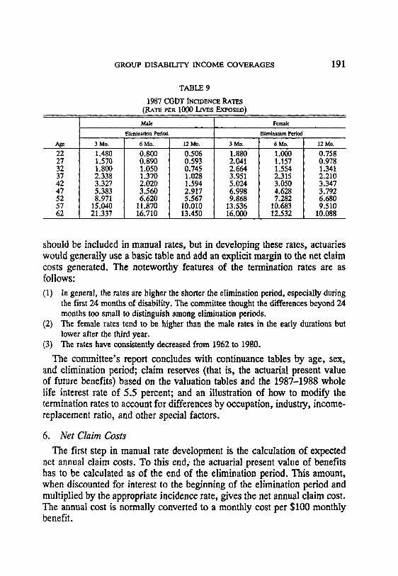
GROUP DISABILITY INCOME COVERAGES
TABLE 9
1987 CGDT INCIDENCE RATES (RATE PER 1000 LIVES EXPOSED)
191
Male Female
Elimination Period Eliminatiou Period Age 3 Mo. 6 Mo. 12 Mo. 3 Mo. 6 Mo. 12 Mo. 22 27 32 37 42 47 52 57 62
1.480 1.570 1.800 2.338 3.327 5.383 8.971
15.040 21.337
0.800 0.890 1.050 1.370 2.020 3.560 6.620
11.870 16.710
0.506 0.593 0.745 1.028 1.594 2.917 5.567
10.010 13.450
1.880 2.041 2.664 3.951 5.024 6.998 9.868
13.536 16.000
1.000 1.157 1.554 2.315 3.050 4.628 7.282
10.683 12.532
0.758 0.978 1.341 2.210 3.347 3.792 6.680 9.510
10.088
should be included in manual rates, but in developing these rates, actuaries would generally use a basic table and add an explicit margin to the net claim costs generated. The noteworthy features of the termination rates are as follows:
(1) In general, the rates are higher the shorter the elimination period, especially during the first 24 months of disability. The committee thought the differences beyond 24 months too small to distinguish among elimination periods.
(2) The female rates tend to be higher than the male rates in the early durations but lower after the third year.
(3) The rates have consistently decreased from 1962 to 1980.
The committee's report concludes with continuance tables by age, sex, and elimination period; claim reserves (that is, the actuarial present value of future benefits) based on the valuation tables and the 1987-1988 whole life interest rate of 5.5 percent; and an illustration of how to modify the termination rates to account for differences by occupation, industry, income- replacement ratio, and other special factors.
6. Net Claim Costs
The first step in manual rate development is the calculation of expected net annual claim costs. To this end," the actuarial present value of benefits has to be calculated as of the end of the elimination period. This amount, when discounted for interest to the beginning of the elimination period and multiplied by the appropriate incidence rate, gives the net annual claim cost. The annual cost is normally converted to a monthly cost per $100 monthly benefit.

192 G R O U P D I S A B I L I T Y I N C O M E C O V E R A G E S
In the absence of having one's own credible claim experience from which to determine termination rates, an appropriate starting point is the set of basic tables (rather than the valuation tables) of the 1987 CGDT. The interest rate may also be greater than the valuation interest rate provided it reflects the company's return on 5- to 10-year investments.
The actuarial present value of benefits is also called a "claim reserve" or "disabled life reserve." One formula for calculating this reserve is given in Appendix H of the committee's report on the 1987 CGDT [20]. Clearly, other approximations are possible. The Society has prepared a diskette to allow the calculation of a continuance table, claim costs, disabled life re- serves, or active life reserves by using any combination of age, sex, elim- ination period, benefit duration, interest rate, or current duration of disability. Calculations can also be performed for nonlevel benefits.
By using the formulas in Appendix H and the values in Tables E-2 and E-3, the claim reserves at duration four months shown in Table E-3 can be converted to claim reserves at duration three months based on the Basic tables and a 5.5 percent interest rate [20]. These are exhibited in Table 10 along with the expected monthly claim costs per $100 monthly benefit ob- tained by applying the (annual) incidence rates shown previously.
TABLE 10
3-MoIcrH ELIMINATION PERIOD; B~_z,~vrrs TO AGE 65
[sst~
'27 37 47 57
Claim F,.t~',rv~ pet $100 al 3 Mo. Mo~aly Clum C.,os~ l~r $I00
Male Female Male Female
3894 4164 0.50 0.70 4965 5196 0.95 1.69 5737 5888 2.54 3.39 4838 4848 5.98 5.40
7. Social Security Disability Income Benefits As emphasized in the introduction, an estimate of the offset for SSDI is
an important component of the manual rate calculation. To be eligible for SSDI, individuals must have a physical or mental condition (1) that prevents them from doing any substantial gainful work and (2) that is expected to last for at least 12 months or is expected to result in death. The elimination period is five calendar months. This definition is stricter than almost all LTD plans during the first two years of benefit period. Benefits are paid until the claimant is eligible for retirement benefits or until the disability

GROUP DISABILITY INCOME COVERAGES 193
ceases. Benefits are based on a career-average formula adjusted for annual changes in average national wages. Benefits are also payable to eligible dependents.
Even though most plans provide a direct offset for SSDI, there are ad- vantages to the claimant who qualifies: liberal vocational rehabilitation ben- efits, eligibility for Medicare benefits (after 24 months), and increased total income when SSDI benefits are increased with CPI while the offset to the LTD benefit is frozen at the original benefit level. Also, Social Security retirement benefits are higher when an individual qualifies for SSDI because then the years of zero salary while disabled do not count in the career average.
The Social Security Act provides that individuals are disabled only if their impairments are so severe that they are unable to do their previous work and cannot, considering their age, education, and work experience, engage in other gainful work. Accordingly, the requirements for benefits for claimants under age 50 are stricter than those for older claimants. They are also stricter for those who are highly educated or possess skills that are transferable to other jobs.
On March 3, 1986, the House Committee on Ways and Means reported on the approval rates for SSDI:
Percenlage Approval Stage Appmvul
1. Initial determination 36% 2. Reconsideration 14 3. Administrative law judge 52 4. Appeals Council 4 5. Federal Court 46
Pelrcnmp ~ c d
27.3% 60.7 29.4 15.3
Camaulative Percentage
36.0% 39.8 48.4 48.6 49.0
Percentage of ToUd
Ai,prov~
73.5% 7.8
17.6 0.4 0.8
These results show that only 49 percent of claimants who apply for SSDI are considered qualified for approval. Anything the insurer can do to help claimants prepare their applications or their appeals (at least to the admin- istrative law judge stage) will increase the claimants' chances for approval and lower the costs of the plan. Only 26 percent of the claimants who are initially rejected take their cases to the third stage, where the approval rate is more than 50 percent. Consultants and attorneys are available to facilitate the appeals.
194 GROUP DISABILITY INCOME COVERAGES
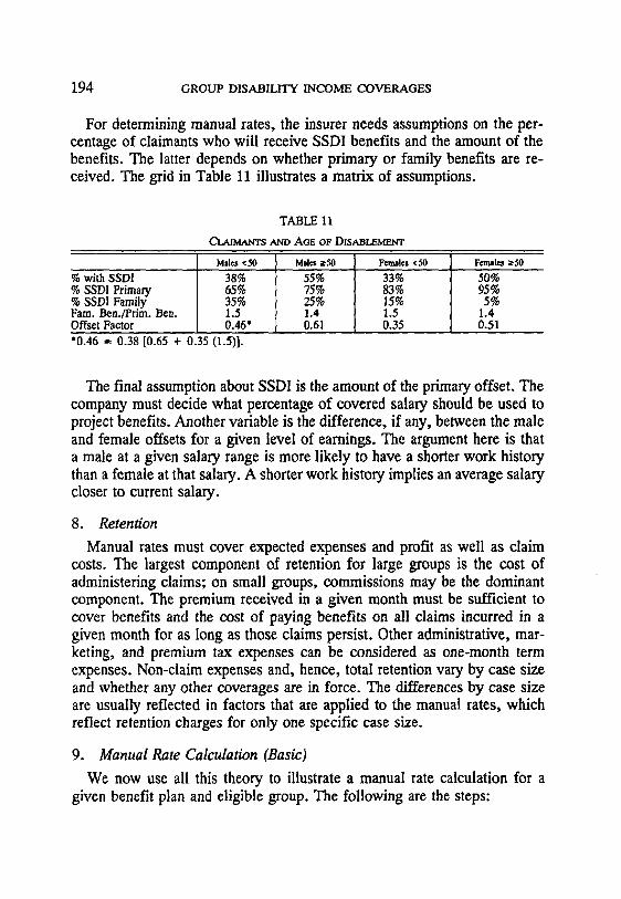
For determining manual rates, the insurer needs assumptions on the per- centage of claimants who will receive SSDI benefits and the amount of the benefits. The latter depends on whether primary or family benefits are re- ceived. The grid in Table 11 illustrates a matrix of assumptions.
TABLE 11
CLAIMANTS AND AGE OF D~SABLEMErCr
Males <50 Males >50 Fondles <50 F©males >50
~b with SSDI 38% 55% 33% 50% ~b SSDI Primary 65% 75% 83% 95% ~b SSDI Family 35% 25% 15% 5% ?am. Ben./Prim. Ben. 1.5 1.4 1.5 1.4 9ffset Factor 0.46* 0.61 0.35 0.51 "0.46 = 0.38 [0.65 + 0.35 (1.5)].
The final assumption about SSDI is the amount of the primary offset. The company must decide what percentage of covered salary should be used to project benefits. Another variable is the difference, if any, between the male and female offsets for a given level of earnings. The argument here is that a male at a given salary range is more likely to have a shorter work history than a female at that salary. A shorter work history implies an average salary closer to current salary.
8. Retention
Manual rates must cover expected expenses and profit as well as claim costs. The largest component of retention for large groups is the cost of administering claims; on small groups, commissions may be the dominant component. The premium received in a given month must be sufficient to cover benefits and the cost of paying benefits on all claims incurred in a given month for as long as those claims persist. Other administrative, mar- keting, and premium tax expenses can be considered as one-month term expenses. Non-claim expenses and, hence, total retention vary by case size and whether any other coverages are in force. The differences by case size are usually reflected in factors that are applied to the manual rates, which reflect retention charges for only one specific case size.
9. Manual Rate Calculation (Basic)
We now use all this theory to illustrate a manual rate calculation for a given benefit plan and eligible group. The following are the steps:

GROUP DISABILITY INCOME COVERAGES 195
(1) Classify the employees according to occupation, for example, executive, salaried, nonsalaried.
(2) Group the employees in each class by earnings, age, and sex. (3) Determine the average monthly benefit for each subgroup in (2).
Let:E = the midpoint of the monthly earnings bracket. P = P(eamings, sex) be the primary SSDI benefit for individuals in this subgroup. f = f(age, sex) be the benefit offset factor. r = the plan's scheduled benefit percentage.
M = maximum covered earnings. t = assumed percentage of claimants qualifying for SSDI.
Then the monthly benefit (B) in a direct offset plan is determined as B = min{rE,rM} - .~.
If the integration level equals s :" r, then B = (t)min{sE-(fit)P, rE, rM} + (1 - t)min{rE, rM}.
(4) Let CC = monthly claim cost per $100 and let IF = industry or class factor. Then the manual rate (R) for each subgroup is
R = (B/IOO)(CC)(IF)/(1 - retention %). The manual rate for the group is the sum of the rates for each subgroup.
10. Manual Rate Calculation (Adjustments)
A company usually adjusts the basic manual rate to account for plan variat ions and group characteristics. Most o f these i tems have already been discussed. For some of them, factors can be determined f rom the TSA Re-
ports or other sources. The important adjustments are listed below.
(1) Additional benefit offsets such as benefits from a pension plan, STD plan, state disability plan, or workers' compensation.
(2) Longer OWN OCC definition period. Decreases termination rates from standard two-year OWN OCC definition.
(3) No freeze on SSDI benefits. Can assume annual decrease in net benefits. This option is rarely used today.
(4) No pre-existing condition exclusion. Increased selection against the plan (for ex- ample, AIDS).
(5) Additional benefits such as cost-of-living increases or survivors' benefits (monthly benefits to widow or widower after death of claimant).
(6) Income replacement ratio. Higher ratio implies higher costs due to less financial incentive to return to work.
(7) Case size. Larger size implies higher costs because it is more likely that the plan is being used as an early retirement vehicle.
(8) Lack of employer contributions. Implies higher costs due to employee selection. (9) Partial disability. Not clear how this affects claim cost, but administrative expenses
will increase. Some insurers use a load of about 5 percent. However, most do not

196 GROUP DISABILITY INCOME COVERAGES
load the rates because they have found that the lower claim costs offset any administrative costs. The question is whether the higher frequency of smaller benefits in the presence of partial disability lowers aggregate costs because benefits would otherwise be paid to some of these individuals as if they were totally disabled.
(10) Residual disability. Greatly increased costs. Some actuaries believe that experience on individual LTD has worsened with the introduction of this benefit on individual polides.
(11) Two-year maximum benefit limitation on disabilities caused by mental, nervous, alcohol, or drug problems. Depending upon the industry, 10 to 25 percent of the claims could fall in this category. The actuary needs to determine what percentage of these claims will actually terminate after two yeats (as physical problems may also be present), and expected claim costs can be lowered appropriately.
(12) U.S. ADEA requirements for continuing benefit payments beyond age 65. In general, the Age Discrimination in Employment Act (as amended) requires that employers not discriminate against individuals over age 40 in hiring, promotion, and compensation (including employee benefit plans). As a result, many employers have concluded that their particular configuration of employee benefit plans re- quires that they (a) continue LTD benefits beyond age 65 for those who become disabled after age 60 and (b) extend coverage to employees who become disabled after age 65.
Because the disability claim rate increases with age, schedules can be con- structed by reducing maximum benefit duration by age in such a way that the actuarial value of benefits for employees between ages a and a + 5 is at least equal to the value for employees between ages a - 5 and a. A schedule with decreasing maximums by age may be used if the actuary can demonstrate equivalence by using accepted actuarial techniques on case data or on a credible body of claim experience. The techniques described in this paper should provide guidance in this area.
One widely used schedule (Federal Register, May 25, 1979) is shown in Table 12.
(13) AIDS. The effect of HIV + on rates can be calculated by adopting the methodology illustrated in the section on STD. Cowell and Hoskius [11] estimate the mortality rate after progression to AIDS is 45 percent in years 1 and 2, 35 percent in year 3, and 25 percent thereafter. The present value of benefits at 5.5 percent interest, per $100 monthly benefit, is $1990 for a 3-month elimination period. A model developed by the author based on [11] gives new AIDS cases in a given year as a percentage of the total number infected with HIV + at the beginning of the year. The modeled percentages rise from 2.5 percent in 1988 to 3.0 percent in 1989 to 4.7 percent in 1992 to 10.8 percent in 1999.

GROUP DISABILITY INCOME COVERAGES
TABLE 12
Age of Disablement Duration of Benefits (last birthday) (in months)
Prior to age 60 60 61 62 63 64 65 66 67 68 69-74
Over ale 74
To age 65 60 48 42 36 30 24 21 18 15 12 6
197
Table 13 is a sample calculation of the effect of AIDS. Based on the author's model, we assume that new AIDS cases currently equal 3 percent of the insureds with HIV + . We assume that (a) disability occurs at the onset of AIDS, Co) the only termination is by death, and (c) these are all additional claims.
TABLE 13
Percentage Pcr~en~.ge HIV + Expected Addiliomd Increase of M_al~ Incidence Costs" C.~ts't in Rate
53% 0.43% 0.59 0.01 1.9% 65 1.25 1.21 0.04 3.3 77 1.08 2.74 0.04 1.5 83 0.37 5.88 0.02 0.3 70% 0.84% 2.55 0.03 I 1.2%
Age Expt~ure
27 18% 37 32 47 28 57 22
Total 100% *Weighted average of male and female costs. tAdditional rate = (% male) (HIM + incidence) (0.03) (1990)/12.
IV. EVALUATING LaD ~XP~RmNO/
The discussion of pricing LTD would not be complete without a review of the techniques used to evaluate LTD experience. This experience evalu- ation can be:
(1) Based on another company's experience to be used, to the extent it is cred~le, to establish rates at the time of the proposal, or
(2) Based on one's own experience to be used, to the extent it is credible, to rerate a case or block of business, or
(3) Based on one's own experience for a retrospective analysis of what actually occurred.
198 GROUP DISABILITY INCOME COVERAGES
LTD experience must be analyzed differently than other types of group health coverages because benefits are paid out over an extended time. Claim reserves and investment income are two features that cannot be ignored. The usual way to evaluate group health experience is to compare the sum of all claims paid during the period plus the change in IBNR (incurred but not reported) to the amount of premium earned during the period. The proper way to analyze LTD is to compare the earned premium during the experience period to the sum of (i) the present value of all payments made on all claims that are incurred during the experience period plus (ii) the present value of the claim reserves held at the end of the valuation period on these claims. If the premium is assumed earned in full at the midpoint of the experience period, the payments and current reserve are discounted back to the midpoint of the experience period. Only in this way can the actuary compare the results in two different experience periods because the later period has less claim runout than the earlier period.
It is also the only way to compare the runout for a given experience period from one year to the next. A loss ratio for a given experience period must be calculated by using present values; otherwise, experience can appear to be worsening even if claimants terminate exactly as expected.
We illustrate the concepts by assuming that we have received complete TBI as described in Section II.B.2. We then explain how to handle situations in which the data are less than complete. Assume the plan has a 9-month elimination period. The valuation date is the end of year 3. The exposure is the same in each year. This example was constructed for years 1 and 2 by assuming (1) 10 new claimants per month with disabilities lasting at least 9 months; (2) a $100 monthly benefit paid at the end of the month; and (3) of the 10 claimants, the first termination occurs at the end of nine months, and the i-th termination occurs i months after the ( i -1 ) th for i = 2, 3, .... 10.
The first step is to split the claims by incurral year and year paid; see Table 14.
Next, the IBNR must be estimated. On a case basis, a shortcut method is often used. Any such method should be supported in the aggregate by lag analysis studies. One method is to apply an expected loss ratio or claim rate to the exposure and subtract paid claims and claim reserves on known claims. A more direct and, possibly, better approach is to apply the loss ratio to the last n months of exposure where n equals the elimination period plus re- porting lag.
Another alternative is to avoid estimating an IBNR by setting back the experience period far enough so that it is safe to assume that all claims have

GROUP DISABILITY INCOME COVERAGES
TABLE 14
199
Year Paid 1 2 3
Total Paid Claims
9,300 91,600 76,300
lneurral Year
9,300 91,600
3
11,160 177,200 100,900 11,160
IBNR 0 0 210,871 Claim Reserve 67,172 137,955 i 71,652 Total Incurred Claims 244,372 238,855 ~ 293,683
74 Number of Active
Claims (End of Year 3) 58 36
been reported. Given the elimination period and the lag in this example, each experience period could be moved back 9 months, provided that the remaining experience is enough to study.
In this example total incurred claims were estimated by taking the ratio of year 1 incurrals paid in year 1 to total year 1 incurrals and dividing the year 3 paid claims by that ratio. Because the claim reserve is known, IBNR is the residual.
Year 2 actually looks slightly better than year 1, but interest has not been taken into account. If the experience study is for prospective use, the actuary will want to discount the benefit stream with an interest rate that is expected to be earned in the future. If the study is retrospective, benefits and the reserve should be discounted by using the actual earned rates in each year.
We discount to the midpoint of the incurral year by using 5.5 percent, which is the rate employed in the reserve calculation. We assume claims are paid in the middle of each year, except the first year. For this year we assume all claims are paid 10-1/2 months after the beginning of the year (4- 1/2 months after the midpoint). The difference between adjusted total in- curred and total incurred is called "the time-value adjustment." (See Table 15.)
TABLE 15
Year I Year 2 Year 3 Fotal Incurred Claims 244,372 238,855 293,684 Firae-Valae Adjustment 21,124 15,607 7,686 ~d~sted Incurred
~laims 223,248 223,248 285,998

200 GROUP DISABILITY INCOME COVERAGES
Now years 1 and 2 are identical. Year 3 appears to be 28 percent worse than the other two.
Suppose we were not given complete claim data. Often one only receives data on claims outstanding on the valuation date. A triangular table can still be constructed based on the information given by reconstructing the paid claims using the known incurral dates and current monthly benefits on active claims; see Table 16. Assume IBNR was orginally obtained by formula and does not change.
TABLE 16
lneumd Year
2
Year Paid 1 4,000 2 49,900 6,000 3 54,00O 77,0O0
Total Paid Claims 103,900 83,000 IBNR 0 0 Claim Reserve 67,172 137,955 Total Incurred Claims ? ?
8,700 8,700
210,871 71,653
?
Clearly, the estimate of incurred claims will be insufficient if the analysis is based only on these data. We must first make an assumption about the claims that have already terminated. Such an inference can be made by using the known claims outstanding and the average persistency of a claim given the termination rate assumptions. Based on this information, a matrix of percentages can be developed by which paid claims should be increased; for example, see Table 17.
TABLE 17
I Inotrcrll Year Year Paid I 1 2 3
1 125% - - 2 100 50% 3 50 25 33%
The actuary then has a more complete triangular table to work with; see Table 18.

GROUP DISABILITY INCOME COVERAGES
TABLE 18
Year Paid 1 2 3
Total Paid IBNR
Claim Rese~
1
9,000 99,800 81,000
189,800 0
67,172 Total Incurred . 256,972 Adjusted Total 234,949
Incurred
lnetm'al Year 2 3
9,000 96,250 11,571
105,250 11,571 0 210,871
137,955 71,653 243,205 . 294,075 227,361 286,400
201
V. VARIANCE AND CREDIBILITY
In determining manual rates for LTD, provision should be made in the rates to cover deviations of interest rates, termination rates, and incidence rates from those assumed in the basic manual rate calculation. There are two sources of deviations. The first is that the assumed rates were biased (either too high or too low) from what is now expected in the long term. The second is that the assumed rates are the expected ones, but there is stochastic fluc- tuation about the mean from year to year. There must be sufficient margin in the premium rates and/or from surplus to withstand these fluctuations with a high degree of probability.
A. Sensitivity of Interest and Termination Assumptions
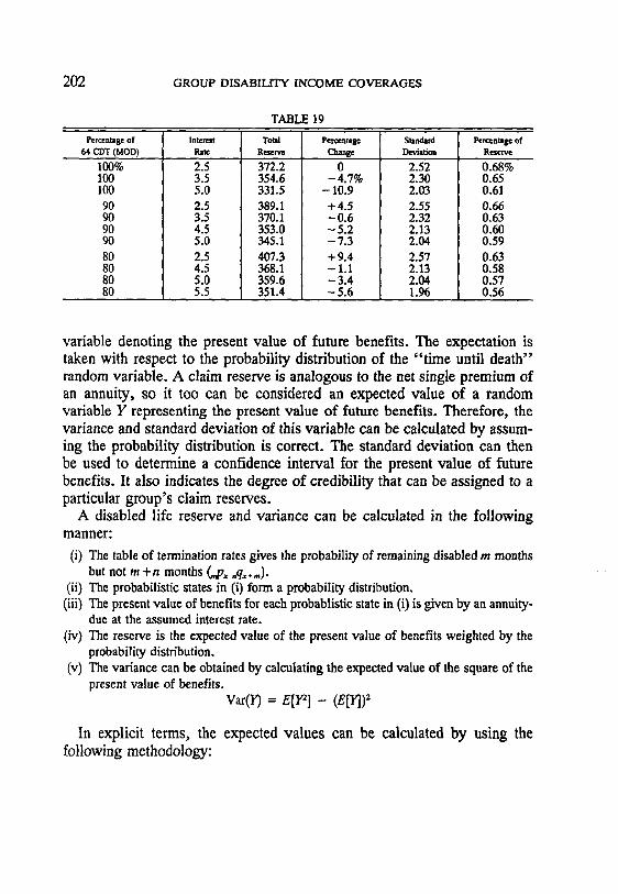
In general, on a mature block of business, claim reserves decrease 4.6 percent for each 1 percent increase in interest rates. They increase by about 4.6 percent for each 10 percent decrease in termination rates, if the interest rate is 2.5 percent. At a 5 percent interest rate, the increase is only 4.1 percent. The effects on a given case or nonmature block of business could be different. The standard deviation of future benefits decreases (as a per- centage of reserves) as termination rates decrease or as the interest rate increases. The calculations summarized in Table 19 were based on the 1964 CDT termination rates, modified downward in the first 12 months.
B. Variance and Standard Deviation
According to Actuarial Mathematics [1] the net single premium of an insurance or an annuity can be interpreted as the expectation of a random
202 GROUP DISABILITY INCOME COVERAGES
TABLE 19
Percentage Of 64 CDT (~OD)
100% 100 100 90 90 90 90 80 80 80 80
lnten:st Total Rate Rt'sev~
2.5 372.2 0 3.5 354.6 -4.7% 5.0 331.5 - 10.9 2.5 389.1 +4.5 3.5 370.1 -0 .6 4.5 353.0 - 5.2 5.0 345.1 - 7.3 2.5 407.3 + 9.4 4.5 368.1 - 1.1 5.0 359.6 - 3.4 5.5 351.4 - 5.6
Percentage Standard Percentag© of Change Deviation R ~
2.52 2.30 2.03 2.55 2.32 2.13 2.04 2.57 2.13 2.04 1.96
0.68% 0.65 0.61 0.66 0.63 0.60 0.59 0.63 0.58 0.57 0.56
variable denoting the present value of future benefits. The expectation is taken with respect to the probability distribution of the "time until death" random variable. A claim reserve is analogous to the net single premium of an annuity, so it too can be considered an expected value of a random variable Y representing the present value of future benefits. Therefore, the variance and standard deviation of this variable can be calculated by assum- ing the probability distribution is correct. The standard deviation can then be used to determine a confidence interval for the present value of future benefits. It also indicates the degree of credibility that can be assigned to a particular group's claim reserves.
A disabled life reserve and variance can be calculated in the following manner:
(i) The table of termination rates gives the probability of remaining disabled m months but not m + n months (,,,p,, ,,qx.m).
(ii) The probabilistic states in (i) form a probability distribution. (iii) The present value of benefits for each probablistic state in (i) is given by an annuity-
due at the assumed interest rate. (iv) The reserve is the expected value of the present value of benefits weighted by the
probability distribution. (v) The variance can be obtained by calculating the expected value of the square of the
present value of benefits. Var(10 = Ella] - (E[Y]) 2
In explicit terms, the expected values can be calculated by using the following methodology:

GROUP DISABILITY INCOME COVERAGES 203
(a) Let Y = Yt~J+, be the random variable representing the present value of $1 per month at duration t for an individual disabled at age x.
(b) Let v = 1/(1 + i). (c) If a disabled life terminates after n months, then Y = Y(n) = 1 + v m2 + v z:~2 +
... + v ("-am with probability ,_,p,,., m2qx+, where n and t are measured in months; n = t, t + l . . . . . 23; t > the elimination period; Y(n) = 0 i f t > 23.
(d) When n > 23, the termination rates are annual rather than monthly. Thus, if a disabled life terminates after k + a years, then
Y = 1:(23) + v"- ' [(12v 1~ + 12v 3r2 + ... + 12v k-~a + 6v k+ta]
with probability k**_dT~÷, q~÷k+o, where k and t are measured in years; k = 0 , 1 . . . . , 6 5 - x - a ; a = 2 if t < 2, otherwise a = t; q~ = 1.
(e) The reserve at age x and duration t equals E[Y], and the Vat(10 is given by the equation in (v) above.
This calculation was applied to a large insurance company's 11,369 active claimants. The standard deviation was only 0.68 percent of the total reserve. Suppose we are valuing a smaller block of data. What would the variance be? Assume that the percentage of claimants and average benefits in each age-duration cell is the same as the company that was studied. Then if the total number of claimants (or reserves) is 100x percent of the company's, the ratio of the standard deviation of reserves to total reserves equals 0.68%/ V'~. See Table 20 for examples. Actually, the standard deviation would be greater than that shown in the table because there is usually only 3-5 years' experience from a prior carrier, and the variance in the reserve of a recent claimant is considerably greater than that of a long-duration claimant.
TABLE 20
x
1 1/6 1/18 1/36 1/72 1/144 1/360 1/720
Number of Claimants Total Resente Standard Deviation (a) (b) (,:) (c).'(b)
11,369 1,895
632 316 158 79 32 16
372.2 mil 62.0 20.7 10.3 5.17 2.58 1.03 0.517
2.52 rail 1.03 0.593 0.420 0.297 0.210 0.133 0.0938
0.68% 1.7 2.9 4.1 5.7 8.1
12.9 18.1
204 G R O U P D I S A B I L I T Y I N C O M E C O V E R A G E S
A more complicated calculation is the calculation of the variance of the present value of benefits from business to be written in the future. In this case, there is statistical fluctuation not only from the termination rates but also from the incidence rates. The expectation of the present value of benefits random variable is the net annual cost that we have used in calculating manual rates. The variance can be calculated by extending the theory pre- sented in Actuarial Mathematics [1].
There are three by-products of this calculation. First, gross premiums can be set so that one has a high level of confidence that the actual present value of benefits will not exceed gross premium. Second, one can determine how much surplus or equity is required to "support" the LTD product line. By "support" we mean there is little likelihood that actual present value benefits will exceed gross premiums plus equity. Third, one can determine the "cred- ibility" of a given number of life years of experience. Both classical and Bayesian credibility are discussed below and detailed examples are given. These examples reflect random fluctuations inherent in the incidence and termination rate assumptions (C-2 risk). Additional margin must be added to protect against other causes of fluctuation such as economic conditions and investment results.
C. Variability of Claims from Current Year's Business
1. Derivation of Formulas for Mean and Variance
(a) Let X~ be the present value of benefits for a given insured. Let N = number of insureds and set S = X1 + X2 + ... + XN. Assuming independence among the insureds, we have
N
e[s] = Z E[,v,] i - 1
and
N
Var (S) = E Var (X~) i - 1
(b) For simplicity we use X instead of X~. We can write
X = / R ,

GROUP DISABILITY INCOME COVERAGES 205
where I = I if the insured is disabled; otherwise I = 0 and R = present value of benefits for a disabled insured. The formulas for the expectation and variance of X are given in Actuarial Mathemat ics [1, Chapter 2].
E[X] = E[E[X]/]]
Var(X) = Var(E[X]/]) + E[Var(Xl/)]
(c) Now R depends on the monthly benefit, the assumed termination rates, and the assumed interest rate. Let u = expected value of the present value of a $1 monthly benefit. Let s 2 = variance of the present value of a $1 monthly benefit. Suppose the monthly benefit varies according to the probability distribution B = B(y), 0 _< y < M. Let b = E[B]. Then
e [R] = uE[B] = ub
Var(R) = (s 2 + u2)E[B 2] - u2b 2
(d) If q is the expected incidence rate, then
Prob{I = 1} = q and Prob{I = 0} = 1 - q.
We can now calculate the expected value and variance of X.
E[X~I = 0] = 0 and E[X]I = 1] = E[R] = ub
Therefore,
Also,
Therefore,
So,
E[E[X[/]I = (1 - q)O + qub = qub
Var(E[X]/]) = q(ub) 2 - (qub) 2 = q(1 - q)u2b 2
Var(X[I = 0) = 0 and Var (X] /= 1) = Var(R)
E[Var(X~] = (1 - q)0 + qVar(R) = qVar(R).
E[X] = qub
Var(X) = q(1 - q)u2b 2 + qVar (R)

206 GROUP DISABILITY INCOME COVERAGES
(e) Therefore, our formulas for E[S] and Var(S) are given below. The for- mula for variance agrees with that on page 210 of Philbrick [15] and in Brender [21.
N N
E[S] = Z E [ X i ] = Eq,u,b, i ff i l i = l
N
Var(S) = ~Var(X,) iffil
N
= ~, {qi (1 - q,)u?b? + q,[(s? + u~)E[B 21 - uZ~b~]t i - 1
2. Required Equity We now apply these formulas to a model of a current block of business
to calculate required equity to support one year's experience.
Annual premium = P = 120,000,000 Expected loss ratio = 87% Average annual premium per insured = 90.
TABLE 21
i
1 2 3 4
Avg.
Age ~ Cenlral Bracket i Age
20-32 I 27 33--42 ~ 37 43--52 47 53--65 , 57
40
Percentage of Covered
Payroll (rj)
Incident Rate per looo (q~)
26% 0.75 33 0.91 24 2.26 17 6.74
2.0
$1/mo. 64 CDT(MOD) @ 2.5%
52.010 2705 5930 59.456 [ 3535 [ 6045 61.406 ] 3771 4224 50.010 J 2501 1198
I 56.4
E[S] = 0.87/°= 104,400,000. The number of lives =N=P/90 = 1,333,333.
Assume that the distribution of monthly benefits is the same for each age bracket. Then
N 4
104,400,000 = E[S] = ~,biu~q, = Nb ~.r,n,qi. i - 1 iffil
This implies that b = 660.

GROUP DISABILITY INCOME COVERAGES 207
Assume that the distribution of B satisfies ~ = ( 0 . 3 ) b . Then E[B 2] = 1.09b z.
So, in this model,
4
V'Var(S) = (Nb 2) ~r,q,[(1.09 - q,)u~ + 1.09s~] i=1
= 2,881,150.
*Required Equity = Q
Choose Q such that
0.99 = Prob{S < E[S l + Q} = Prob [ ~ <
Assuming that S follows a normal distribution [1, chapter 2], we can set Q / X / V - ~ -- 2.326. Then
Q = 6,805,276 -- 5.7% of premium
In addition to the required equity to support the current year's business, the company also needs to hold equity to support the current claim reserve on prior years' business. For 99 percent confidence, on the mature block of business discussed above, equity of (2.326)(0.68%) = 1.6% of reserve is required.
D. Pricing Example
(a) Assume 1000 insureds age 47 with a monthly benefit distribution sat- isfying b = E[B] = 660 and E[B 2] = 1.09 b 2. Assume the values in Table 21. Then
E[S] = Nqub = (1000)(0.00226)(61.406)(660) = 91,593
Var(S) = Nqb 2 [(1.09 - q)u 2 + 1.09s 2] = 8.57070 x 109
= 92,578
Choose premium P such that 1000P = E[S] + ~ .
Then Prob [S < 1000P} = 0.84.
P = 184.17

208 GROUP DISABILITY INCOME COVERAGES
(b) Suppose our assumption for q = 0.00226 was wrong and should have been given by the 1987 CGDT = 0.00356 = q'. Then
E[S'] = Nq'ub = (1000)(0.00356)(61.406)(660) = 144,280
Var(S') = Nq'b 2 [(1.09 - q')u 2 + 1.09s 2] = 1.34931 x 10¹⁰
~ = 116,160
Choose premium P' such that 1000P' = E[S'] + ~ .
P' = 260.44
The proper premium should have been 260.44 (41 percent increase); however, we charged only 184.17. What is the probability that we do not lose money at 184.17 given that frequency is really q'? Assuming S' has a normal distribution about its mean, we have
ooo,_ Prob{S' < IO00P} = Prob < ~ j = 0.63
E. Credibility
Let S0 = claims in year i and let S = average claims over n years:
= (l/n) ~ S0. lml
Assume that the S~ have the same probability distribution. Denote S0 by S. Then E[S] = E[S] and Var(S) = (l/n) Var(S).
Define: Confidence = Prob {]S-E[S]I < aE[S]}where a > 0; equivalently,
Prob~I~ - EtS]I aEtTS] 1 Confidence = l VX/'V~ar(S) < ~ J
If we assume the exposure for N lives is distributed as in Section V.C.2, we have
E[S] = 78.3N and x/var(s) = 2495 X/(N/n).
Assuming that S has a normal distribution, we obtain the following confi- dence percentages for given N, n, and a as shown in Table 22.

GROUP DISABILITY INCOME COVERAGES
TABLE 22
t Ycm of r:x~.'en~ (.) Conf':dcnee Pctommg~'s (a - 0.05)
250 2 3 4 4 500 3 4 5 6
1,000 4 6 7 8 2,000 6 8 10 12 4,000 8 12 14 16 8,000 12 16 20 23
16,000 16 23 28 32 32,000 23 32 39 44 64,000 32 44 53 59
128,000 44 59 69 76 256,000 59 76 85 90 512,00(} 76 90 96 98
Con~dcno: Perc~alages (a = 0.I0)
250 4 6 7 8 500 6 8 10 12
1,000 8 12 14 16 2,000 12 16 20 23 4,000 16 23 28 32 8,000 23 34~2 39 44
16,000 32 53 59 32,000 44 59 69 76 64,000 59 76 85 90
128,000 76 90 96 98 256,000 90 98 100 100 512,000 98 100 100 100
5 7 9
13 18 28 36 49 65 81 94 99
9 13 18 26 36 49 65 81 94 99
100 100
209
1. Classical Credibility
In classical credibility theory, the confidence percentages depend upon an assumed probability distribution for total claims. They can be interpreted as the degree of credibility to be given to the experience of an individual risk relative to the expected experience of the class to which the risk belongs. On another plane, they can be interpreted as the degree of credibility to be given to the experience of a particular class relative to the expected expe- rience of the whole block of business. In experience-rating calculations, the confidence percentages are the weights Z used in the equation for expected claims for an individual risk:
Expected claims = Z (mean of the observed claims for the individual risk) + (1 - 2,) (expected claims for the class).
The expected claims for the class are the net claim costs determined from the manual rate calculation, where the net claim cost equals the manual rate
210 GROUP DISABILITY INCOME COVERAGES
less retention, margin, and risk or profit charge. In practice, 100 percent credibility is given for many fewer life years' experience than Table 22 would warrant.
2. Bayesian Credibility In Bayesian credibility, the subjective factor " a " does not have to be
specified, nor does a probability distribution for claims have to be assumed. As pointed out by Philbrick [15], credibility increases with: (1) Increasing number of observations (that is, number of experience years), (2) Decreasing process variance [that is, Var(S)], and (3) Increasing variance of the hypothetical means (that is, variance of the expected
claims of all the groups in the class).
In Bayesian credibility, the credibility factor Z in Section V.E.1 is given by
n (*) n + K
where n = number of experience years and K = expected value of process variance
variance of the hypothetical means"
"Process variance" is the variance of the aggregate claims generated by an individual risk, which may represent a combination of risk factors. In the example that follows, it equals Var(S). The "hypothetical mean" refers to the expected aggregate claims generated by an individual risk, that is, E[S].
We have followed Philbrick [15] by referring to (*) as intrinsic to Bayesian credibility. He distinguishes the latter from the pure Bayesian model. Herzog [12] refers to (*) as Biihlmann's credibility formula, which he also distin- guishes from the pure Bayesian model. However, as proved in Biihlmann [3] and Herzog [12], Z as defined in (*) is the coefficient of S in the "best" linear approximation to the pure Bayesian model of expected claims (where
is the average observed claims over n years).
Example Suppose that we have n years of experience on a newly insured group G
(that is, an individual risk) whose demographics and coverage distribution match the data in Section V.C.2. Let Si be a random variable representing the claims in year i. After adjusting for year-to-year differences in exposure (that is, covered salary), we assume the Si's are independent, identically distributed random variables. Let S be the common distribution. Let S be
GROUP DISABILITY INCOME COVERAGES 211
the average observed claims over n years after adjusting for annual differ- ences in exposure.
We want to project the expected claims for G in the following year. To do so, we consider all the existing groups {Gk} in the same industry/occu- pation class as G. The quantity E[S] is determined by applying the manual loss ratio times the manual rate (that is, it equals the manual rate less reten- tion, margin, and risk charges). If we assume the manual rate is determined by the experience of the class, then E[S] is the expected claims for the class. Thus,
expected claims for G = ZS + (1 - Z) E[S],
where Z is defined by (*). Based on the calculation in Section V.C.2, we have for N lives
E[S] = 78.3N
Var(S) = (2495)2N.
Given realistic salary and Social Security assumptions, we show that a man- ual rate of $0.45 per month of $100 of covered salary is consistent with the data in Section V.C.2.
(a) Recall that the expected monthly benefit is $660 or $6.60 per $100. How does $1 of benefit relate to covered payroll? Assume the average benefit percentage is 60 percent, the average percentage of claimants with SSDI is 68 percent, and the average SSDI benefit is 30 percent of covered salary. Then $1 benefit = [0.60 - (0.68)(0.30)](covered salary) -- 0.396 (covered salary).
With an expected loss ratio of 87 percent, we can relate the expected benefits per life (78.3) to a monthly rate:
[(78.3)(0.396)]/[(6.60)(12)(0.87)] = 0.45 per month of $100 covered salary.
(b) Alternatively, recall that the average annual premium is $90. With an average annual covered salary of $20,000 or $1667.67 per month, the monthly rate would be 90/200 = 0.45. This is consistent with (a) because 660/1667.67 = 0.396.
Our objective is to calculate Z, or equivalently, K. We need to use the experience of the groups in the class, but each group has different distri- butions by age and covered payroll. We will describe one approach for putting them on the same basis.
The manual rate per $100 of covered salary for group G is 0.45. For each group Gk, we can calculate an experience rate Xk such that the ratio of Xk to 0.45 equals the ratio of (1) to (2) where:
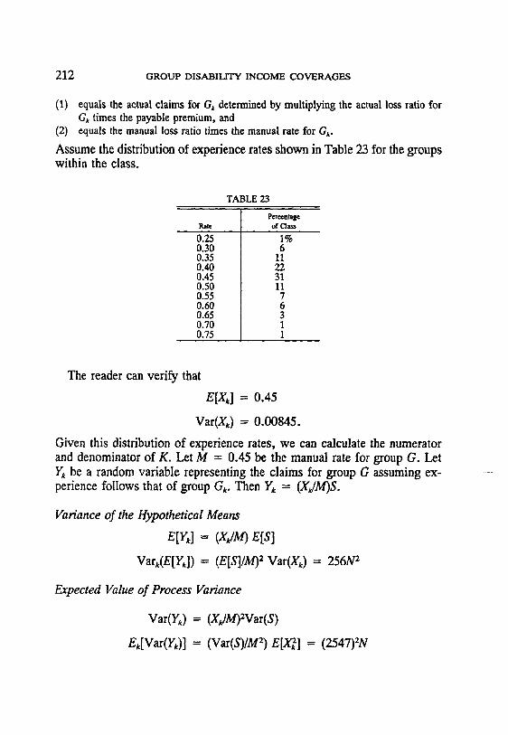
212 GROUP DISABILITY INCOME COVERAGES
(1) equals the actual claims for G, determined by multiplying the actual loss ratio for Gk times the payable premium, and
(2) equals the manual loss ratio times the manual rate for G~,.
Assume the distribution of experience rates shown in Table 23 for the groups within the class.
TABLE 23
Petectltage P,~le of Qass
0.25 1% 0.30 6 0.35 11 0.40 0.45 31 0.50 11 0.55 7 0.60 6 0.65 3 0.70 1 0.75 1
The reader can verify that
E[X,] = 0 .45
Var(Xk) = 0 .00845 .
Given this distribution of experience rates, we can calculate the numerator and denominator of K. Let M -- 0.45 be the manual rate for group G. Let Yk be a random variable representing the claims for group G assuming ex- perience follows that of group Gk. Then Yk = (XJM)S.
Variance of the Hypothetical Means
E[Y,] = E[S]
Vark(E[Vk]) = (E[S]/M) 2 Var(Xk) = 256N ~
Expected Value of Process Variance
Var(Y~) = (X~/M)War(S)
Ek[Var(Yk)] = (Var(S)/M 2) e[x~k] = (2547)2N

GROUP DISABILITY INCOME COVERAGES 213
Credibility Therefore, K = (2547/16)2/N. Thus, we obtain the credibility factors shown in Table 24 for a group with
N lives and n years of experience.
TABLE 24
BAYESIAN CREDIBILITY
] Years of E.xp~ence (n) Ltv~ (N) : 1 2 3 4 5
250 1 2 3 4 5 500 2 4 6 7 9
1,000 4 7 11 14 16 2,000 7 14 19 24 28 4,000 14 24 32 39 44 8,000 24 39 49 56 61
16,000 39 56 65 72 76 32,000 56 72 79 83 86 64,000 72 83 88 91 93
128,000 83 91 94 95 96 256,000 91 95 97 98 98 512,000 95 98 98 99 99
VI. REGULATORY ISSUES
Few, if any, states have statutory requirements for group STD or LTD reserves. Most companies use their own experience for STD without a dis- count for interest. For LTD, most use a modified version of the 1964 CDT; however, a few companies have adopted the 1987 CGDT or a modification of it. The NAIC has recommended use of the latter table together with the statutory whole life interest rate effective in the year of disablement. Com- panies may base reserves on their own experience for claims within the first two years of disability. In Canada the valuation actuary is responsible for making good and sufficient provisions for reserves.
Before 1987, U.S. companies used the same reserves for tax purposes as for statutory purposes. The 1986 Tax Act changed that for many companies. The provisions of this act require that reserves for disability income reflect the insurer's mortality and morbidity experience. The general rules of Sec- tion 807(d) apply except that the whole life interest rate used for discounting is the rate in effect for the year in which the loss occurred rather than the year in which the contract was issued. A company cannot deduct reserves

214 GROUP DISABILITY INCOME COVERAGES
for an accident year that are greater than the statutory unpaid losses included in the company's statutory statement.
The 1987 Tax Act raised the minimum interest rate to a five-year average of the applicable Federal mid-term rates with no reduction for margin.
Finally, the federal income tax code can affect the design of disability income plans. The tax implication of disability benefits should be taken into account in benefit design and in determining employee versus employer contributions. With changes in the tax code, the prior claim experience may not be representative of the future.
REFERENCES
1. BOWERS, N., GERBER, H., HICKMAN, J., JONES, D., AND NESBrr'r, C. Actuarial Mathematics. Itasca, I11.: Society of Actuaries, 1986.
2. BRENt)ER, A. "Required Surplus for the Insurance Risk for Certain Lines of Group Insurance," TSA XXXVI (1984): 9-47.
3. BOHLMANN, H. MathematicalMethods in Risk Theory. New York: Springer-Verlag, 1970.
4. COMMITTEE ON GROUP LIFE AND HEALTH INSURANCE. "Group Long-Term Dis- ability Insurance," TSA 1984 Reports (1988): 243-300.
5. COMMITTEE ON HEALTH INSURANCE. "II. Experience under Individual Loss.of- Time Policies, 1980," TSA 1982 Reports (1985): 217-63.
6. COMMITI~E ON LWE ANt) HEALTH INSURANCE. "I. Group Weekly Indemnity In- surance," TSA 1972 Reports (1973): 249-57.
7. COMMITTEE ON LIFE AND HEALTH INSURANCE. "II. Group Weekly Indemnity Insurance," TSA 1980 Reports (1981): 117-28.
8. COMMITTEE ON LIFE AND HEALTH INSURANCE. "II. Group Long-Term Disability Insurance," TSA 1981 Reports (1983): 245-311.
9. COMMXTrEE ON LIFE ANt) HEALTH INSURANCE. "I. Group Weekly Indemnity In- surance," TSA 1982 Reports (1985): 267-342.
10. COMMITrm~ ON LIFE Am) HEALTH INSURANCE. "'II. Group Long-Term Disability Insurance," TSA 1982 Reports (1985): 277-342.
11. COWELL, M.J. AND HOSmNS, W.H. "'AIDS, HIV Mortality and Life Insurance." In The Impact of AIDS on Life and Health Insurance Companies: A Guide for Practicing Actuaries, Report of the Society of Actuaries Task Force on AIDS. Re- printed in TSA XL, Part II (1988): 909-72.
12. HERZOO, T.N. "Credibility: The Bayesian Model Versus Bfihlmann's Model," TSA XLI (1989): 43--82.
13. MmLER, D. "Group Weekly Indemnity Continuation Table Study," TSA III (1951): 31-67; Discussion, 505-29.
14. New Group Disability Insurance. Washington, D.C.: Health Industry Association of America, 1986.

GROUP DISABILITY INCOME COVERAGES 215
15. PHILBRICK, S.W. "All Examination of Credibility Concepts," Proceedings of the Casualty Actuarial Society LXVIII (1981): 195-219.
16. "Report of the Committee to Recommend New Disability Tables for Valuation," TSA XXXVII (1985): 449-601.
17. "Report of th~ Life and Health Actuarial (EX5) Task Force," NAIC Proceedings 1 (1985): 437-38.
18. ROSENBLOOM AND HALLMAN. Employee Benefit Planning. Englewood Cliffs, N.J.: Prentice Hall, 1986.
19. "Salaried Employees' LTD, STD Plans: 1986 Surveys From Hewitt Associates, Mercer-Meidinger-Hansen," Spencer's Research Reports 323.5-323.8, March 1988.
20. SOCmTY OF ACrUAR~ES COMMrrrEE To RECOMMEND NEW D~sAa~LrrY TABLES FOR VALUATION, "'Group Long-Term Disability (GLTD) Valuation Tables," TSA XXXIX (1987): 393-457.
21. Source Book of Health Insurance, 1988 Update. Washington, D.C.: Health Industry Association of America, 1988.

DISCUSSION OF PRECEDING PAPER
CHARLES S. FUHRER:
Dr. Goldman is to be commended for bringing many of the methods used by group underwriters and actuaries working in the field of disability income insurance to the attention of the readership of the Transactions. The descrip- tive parts of the paper are useful and worth reading. I found some of the formulas and statistical material to be unclear.
I. SOCIAL SECURITY DISABILITY INCOME (SSDI)
AND BENEFIT CALCULATIONS
Manual Rate Calculation (Basic) [Section III-B9, item (3)] contains two formulas for the monthly benefit B. I believe that both formulas should have excluded negative benefits. This may seem like a trivial point, but it is not. The exclusion of negative benefits requires the splitting of the formula into three terms: (1) for family SSDI benefits, (2) for primary SSDI benefits, and (3) for no SSDI. The first two terms cannot be combined into one using a weighted "offset factor" because the resulting benefit may be negative for family SSDI. Thus the second formula becomes:
B = tF[min(sE -- F, rE, rM}] ÷ + tp[min(sE - P, rE, rM] +
+ (1 - t)rain{rE, rM}
where t r= probability of claimants qualifying for family SSDI; t,,,= probability of claimants qualifying for primary only SSDI; t = r e + t v; F = the family SSDI for individuals in the subgroup; and x* = max(x,0) is the positive part ofx .
Incidentally, many plans have different maximum earnings for integration and different integration levels for primary versus family SSDI. Thus the formula will be more complicated:
B = tF [min{rEs, reEe - P, rrEF - F}] +
+ t~, [min{rEB, reEp - P}]+ + (1 - t ) rEn
where EB = min{E, Ms}; Ee = min{E, Me}; EF = min(E, MF}; Ms = the maxi- mum covered earnings without integration; Me = the maximum covered earn- ings for primary integration; Mr = the maximum covered earning for full
217

218 GROUP DISABILITY INCOME COVERAGES
integration; re = the integration level for primary benefits; and rF = the in- tegration level for family benefits. I have not seen plans with r, re, and re all different. I have seen primary only plans (re=0) and plans with r=re<_re.
The above formulas depend on the actual earnings E for each individual. Because of the exclusion of negative benefits, there is some inaccuracy in grouping individuals into monthly earnings subgroups. Fortunately, the availability of data-processing equipment has allowed most insurers to use each employee's actual earnings when estimating benefits for calculating premium rates.
The above formulas are actually for the E(B), where B is the random variable representing an individual's monthly benefit. These formulas in- clude the random variables F and P. These are effectively random variables because the SSDI benefit depends on each individual's covered earnings history, which is usually unknown to the insurer. Presumably, the insurer will estimate P (and therefore F) for a given earnings level and age by estimating past earnings, based on assumed patterns of inflation and pro- motions. These are, of course, actually estimates of E(P) and E(F). In the formula above these estimates of E(P) and E(F) cannot be inserted for P and F, respectively, because:
E[min{rEs, reEe - P}]+ > [min{rEs, reEe - E(P)}] +
and
E[min{rEB, reEe - P, reEF - F}] + > [min{rEB, reEe - P, rvEe - E(F)}] +.
In other words, in order to get E(B), we cannot use E(P) or E(F), because E(P) is calculated without setting those values of P that are less than reEe equal to reEe, and therefore negative benefits are effectively included in the calculation of the expectation. Some insurers have adjusted for this by roughly estimating values to use in the above equations that are slightly lower than E(P) and E(F). A more precise method would assume some distribution for prior earnings and calculate the resulting distribution of SSDI benefits and a correct E(B). A slightly easier technique would be to estimate the mean and variance of past earnings, calculate the resulting mean and variance of the SSDI benefits, and calculate the E(B) using the normal approximation.
In calculating the probability that a claimant will not receive SSDI ben- efits, it is also necessary to include the probability that individuals were not employed long enough to be eligible.

DISCUSSION 219
One must also recognize that the probability of the disability being ap- proved for SSDI benefits increases as the time since incurral of disability increases; that is, short-term claimants have a lower rate of offset. Some of the reasons for this are: (1) the disability may not qualify because of the one-year or death provision in the SSDI law; (2) the disability may qualify only because of a two-year OWN-OCC provision of the LTD contract; (3) the longer the individual is on claim, the more likely that his/her appeal process will be fully pursued; and (4) of course, if the elimination period of the plan (for example, three months) is less than that under SSDI, then some early benefits are never offset. In general, a very high percentage of claims is offset after five years from disability. Thus, in calculating E(B), the value of t would be the proportion offset at each duration, weighted by the product of the present value and the probability of payment at that duration. The ratio of tF to t would also change with duration from disability.
The determination of expected benefits under offset plans is very com- plicated. Nevertheless, the situation has improved considerably over the last few years. Now, almost all plans have the so-called "social security freeze" (required by law in most states) that specifies that the annual SSDI cost-of- living adjustments, which occur after a claimant's SSDI payments com- mence, will not further reduce his/her benefits. About fifteen years ago most LTD plans did not have this freeze provision. Nonfreeze benefits require the estimate of SSDI cost-of-living adjustments many years into the future. Fur- thermore, because all but the oldest claimants could eventually have zero benefits, the problem mentioned above (not including negatives into the calculation of expectations) would occur more often. The actuary still needs to be aware of the problems inherent in nonfreeze benefits for claim reserves that include claims incurred many years ago. Also, there may be self-insured plans, exempt from state regulation, that have nonfreeze benefits.
Most of these remarks relate specifically to the U.S. SSDI program. Dif- ferent methods might be necessary for the Canadian Pension Plan or an employer's pension plan that has disability benefits. Offsets for an employ- er's pension plan can make the calculation of premiums for a proposed LTD plan extremely complicated. The insurer needs to understand the provisions of the pension plan's disability benefits and to be aware of the pattern of approvals for these benefits. Many of these plans base the size of the benefits on years of service, data that insurers would otherwise not need.

220 GROUP DISABILITY INCOME COVERAGES
II. DISABLED LIFE RESERVE CALCULATION
Section V-B describes a method of calculating the disabled life reserve and variance. I think the description contains some ambiguities and less- than-well-defined terms. For example, what is a "probabilistic s tate"? Also, in (a), what is selected at duration t in the expression Yx+i,l ? In (c) and (d), functions Y(n) and Y(k) are defined; yet Y(n)--b Y(k) when n = k. In fact, in (d), I:(23) is used. Which Y is it? In (a) a random variable represents the present value of expected benefits. I assume that it represents the present value of benefits. The quantities im and vm are defined even though vm is merely equal to v 1/~2.
My interpretation of the passage under discussion is as follows:
Let Yv, I+, be the random variable representing the present value of $1/month of benefits at duration t for an individual disabled at agex. Let T0,1+ , be the random variable equal to the time after duration t that a life disabled at age x and still disabled at x + t remains in a disability benefit status. Assume that t=k/12 for some integer k>0. Also assume that t - elimination period. Then
Y~l+t "~ ~ vat2 j=O
where n is the unique integer for which:
n -< 12To, I+ , < n + 1.
The distribution of T[,l÷ , is calculated from rates of termination of disability:
Pr{n/12 < Tt.,l+ , < (n + I)/12} = nl12Pf=]+* l/t2q[xl+t+n/12.
Since only some values of q are available, approximations need to be used.
I11. THE MONTHLY BENEFIT RANDOM VARIABLE
I would like to clarify the value Var(B) in the calculation of the variance of a year 's claims in Sections V-C1 and V-C2. I had some difficulty fol- lowing this part of the paper. In the paper B is defined in subsection (c) as a probability distribution that is equal to a function of a quantity y , with 0-<y-<M. I interpret this to mean that B was the random variable equal to the monthly benefit and that O<B<M. M is also undefined, but I believe it is intended to be the maximum monthly earnings as defined in Section III- B9(3). If so, perhaps it would be better to say that B<_rM. The author never defines u, s, b, q, R, and B. I assume that, for notational simplicity, u = ui, s2=s~, b=bi=E(Bi), I=I~, q=qi, R=Ri, and B=Bi, as the author states
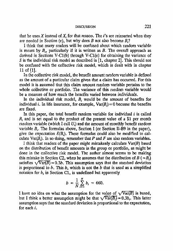
DISCUSSION 221
that he uses X instead of X~ for that reason. The i 's are reinserted when they are needed in Section (e), but why does B not also become B~?
I think that many readers will be confused about which random variable is meant by Bi, particularly if it is written as B. The overall approach as derived in Sections V-CI(b) through V-CI(e) for obtaining the variance of S is the individual risk model as described in [1, chapter 2]. This should not be confused with the collective risk model, which is dealt with in chapter 11 of [1].
In the collective risk model, the benefit amount random variable is defined as the amount of a particular claim given that a claim has occurred. For this model it is assumed that this claim amount random variable pertains to the whole collective or portfolio. The variance of this random variable would be a measure of how much the benefits varied between individuals.
In the individual risk model, B~ would be the amount of benefits for individual i. In life insurance, for example, Var(B~)= 0 because the benefits are fixed.
In this paper, the total benefit random variable for individual i is called R~ and is set equal to the product of the present value of a $1 per month random variable (which I call Ui) and the amount of monthly benefit random variable Bi. The formulas above, Section I (or Section II-B9 in the paper), give the expectation E(B~). These formulas could also be modified to cal- culate Var(B,). In so doing, remember that P and F are also random variables.
I think that readers of the paper might mistakenly calculate Var(B) based on the distribution of benefit amounts in the group or portfolio, as might be done in the collective risk model. The author almost seems to be making this mistake in Section C2, when he assumes that the distribution ofB (=Bi) satisfies ~ = 0.3b. This assumption says that the standard deviation is proportional to b. This b, which is not the b that is used as a simplified notation for bj in Section C1, is undefined but apparently
1 ~ b =~[~,bi = 660. i - 1
I have no idea on what the assumption for the value of ~ is based, but I think a better assumption might be that ~ = 0.3bi. This latter assumption says that the standard deviation is proportional to the expectation, for each i.

222 GROUP DISABILITY INCOME COVERAGES
The term:
IV. THE FORMULA FOR
N _ q2 u~ b 2
i -1
that appears in the formula for Var(S) in Section V-CI(e) becomes 4
- N b 2 ~,, ri q2 u 2 i=l
in the formula for ~ in Section V-C2. I think that these two expres- sions would be equal only if bi were constant over the whole portfolio. In practice, it would not be very difficult to sum the actual values of this term.
V. THE FORMULAS FOR E(R) AND VAR(R)
The formulas for E(R) and Var(R) in Section V-Cl(c) are true only if the random variables U (that I defined, Section III) and B are independent. In general, as discussed in Section I above, these are not independent.
VI. THE TOTAL VARIANCE OF THE PORTFOLIO
In Section V-C2 the author calculates the total variance of the current year's business. This calculation would be improved by adding the variance of expected claims between groups. The model is that each group has an unknown parameter, O, that is also a random variable. It is easy to show that if S is the total claims for the group, then:
War(S) = E[Var(SIO) + Var[e(slo)].
The calculation for the required equity, in the paper, uses the first term only. The author estimates the second term in Section V-E2 and calls it the "'var- iance of the hypothetical means." This quantity is used in this later section to calculate the linearized Bayesian credibility. Nevertheless, it should not be looked upon as a quantity that can be used for credibility calculations only. Group insurance portfolios exhibit larger variances than the sums of the variances of the individual benefits. Group insurance portfolios do not contain a homogeneous set of individuals. In any case, if this quantity is assumed not to be part of the variance, then there is really no reason not to use zero credibility.
If we use the author's numbers and assume that all the groups consist of, for example, 10,000 employees, then Q becomes 6.6 percent of premium.

DISCUSSION 223
If we assume that the whole block of business is one group, then Q becomes 41.7 percent of premium. This last assumption is obviously incorrect, but a single employer may constitute the bulk of an insurer's coverage.
Vll. CLASSICAL CREDIBILITY AND OTHER CREDIBILITY METHODS
When an insurer is faced with the problem of developing the expected claim costs for a prospective group, I believe that nothing is superior to using the conditional expectation of claims given all available data. The credibility method presented in Section V-E2 is the best (in the sense of least squares) linear estimate of the conditional expectation of a group's claims given its past claims. There are a number of ways one might improve this method. One method might involve using some other criterion than least squares as a measurement of the quality of the estimator. A second way would be to use other than linear approximations. Some nonlinear credibility formulas have been proposed; see, for example, Jewell and Schneiper [7] or Fuhrer [4]. If we knew more about the distribution, we could actually estimate the conditional expectation. This true "credibility premium" is mentioned in Bi.ihlmann [2]. A third improvement might be to use more data. One such method would use the number as well as the size of the claims in the group's claim history. Herzog [5] develops such a formula as the linear Bayesian credibility estimate of the number of claims multiplied by the same kind of estimate of the size of claims. Jewell [6] solves this problem by using the formula:
(estimated claims) = Z1 (number of claims) + Z2 (total claims) + (1 - Z1 - Z2)(portfolio rate).
See also Btihlmann [3]. Some work needs to be done to modify this method to adjust for incurred claims, including estimated claim reserves, in long- term disability insurance.
With these methods in mind, I can see little justification for using classical credibility for rating a group. It relies on the subjective selection of confi- dence percentages, and the resulting estimate is not optimum. Perhaps the classical method has some place in the evaluation of the size of experience for a particular rating class. It is possible that it might also be more accept- able to a regulator. Philbrick [8, Summary, p. 219] comes to the same negative conclusions about classical credibility.

224 GROUP DISABILITY INCOME COVERAGES
ii. FORMULA FOR VAR[ ]
In the part of Section V-E before V-E1, the author uses the formula Var[S]--(1/n)Var(S). This equation is correct only if the Sz's are uncorre- lated, which is not assumed in this part of the paper.
IX. BAYESIAN CREDIBILITY
I found the development of the Bayesian credibility method in Section V- E2 unclear. For example, S is defined as a distribution, but then treated as a random variable. Also, I have a no idea what Vark(E[Yk]) or E[Var(Y)] means.
Si is defined as the random variable equal to claims for year / (0_<i_<n) for group G. The Si's are assumed to be independent and identically distrib- uted (rid) random variables after adjusting for differences in exposure (cov- ered salary). I am not sure how this adjustment is to be made; perhaps we should divide by the covered salary so that the S~'s are actually defined as the claims per dollars of covered salary. S is then defined as the average of the Si's (also adjusted for exposure). Then the author uses the equation:
(F.xpected claims for G) = Z:~ + (1 - Z)E[S].
I assume that the claims for G in the coming year (call them S,+~) are also iid with the other Si's ( l< i<n) . Otherwise, we would have the strange situation in which the S~ continued for n years iid and then suddenly changed. If S,+t is iid with St ... S,, then E[S,+t] =ElSe] for l < i < n . More specifically E[Sa+I]S1 . . . Sn] =E[S i ] and thus Z=O.
An alternative explanation can replace the part of the paper from "Ex- ample" until Table 23:
Let St be the random variables equal to the manual loss ratio for a group in year i (l<i<_n + 1). We are given the actual loss ratios that occurred in years 1 through n. We will use the estimate E[S,+ 1]S~ ... S,,] ~Z~ + C, where Z and C are constants and
5 =1- ~S~. n i - I
If we minimize the expected squared error of this estimate and assume that E(S~) =E(Sj) = ~ for every l<-i , j<n + 1, then it can be shown that C= (1-Z) lx and
Z = Cov( S, S, ; i )/V ar( S ).
If we also assume that for a parameter ~, (S~[~) l<i<n +1 are independent and identically distributed, then Z =n/(n +I0, where K=E[Var(SJ~)]Nar[E(S~IO)]. Here

DISCUSSION 225
the parameter ~ is assumed to be a random variable (constant over time) that is associated with each group. Also, note that Var(Sj)= g[Var(S~l~)] + Var[E(S,t~)].
X. THE VARIANCE OF THE HYPOTHETICAL MEANS
The description above (which is consistent with all the other credibility references, including Philbrick [8], Herzog [5], and Biihlmann [2]), of the linearized Bayesian method indicates that the value of K is the ratio of the two components of the variance of S~, that is:
Var(Si) = E[Var(S,l'O)] + Var[E(Sil'0)].
K is not equal to the ratio of two components of some other random variable Yk = (XJM)S, as stated in the paper.
Here is one way to estimate Var[E(Si[~)]. The distribution of "experience rates" in Table 3 is actually the distribution of group net manual loss ratios in the class, multiplied by a constant. Thus it actually represents the distri- bution of S~ for a randomly selected group G. Now using the formula:
Var(S,) = E[Var(S, la3)] + Var[E(S,[~)]
we have
therefore
and
256N 2 = 24572N + Var[E(S, IO)];
Var[E(S, lO)] = 256N 2 - 25472N,
25472N 25472 g - - - --- 256N 2 - 25472N 256N - 25472"
Of course, for small N, Var[E(Si[~)] < 0, which is known to be a problem when using this kind of estimate. Nevertheless, the distribution of Table 23 has far too low a variance for the distribution of loss ratios of groups in a class in one year. I would expect many groups to have zero claims as well as many to have 200 percent or 300 percent loss ratios. Also, the problem that I pointed out in Section IV above would tend to overstate E[Var(S~[~)]. Actually, the author's estimate of Var[E(Stl~)] = 256N 2 does appear quite reasonable. I wonder whether Table 23 was derived from actual data or was constructed to produce a reasonable Table 24.

226 GROUP DISABILITY INCOME COVERAGES
REFERENCES
I. BOWERS, N.L. JR., GERBER, H.U., HICKMAN, J.C., JONES, D.A., AND NESBITT, C.J. Actuarial Mathematics, Itasca, Ill.: Society of Actuaries, 1986.
2. BOHLMANN, H. Mathematical Methods in Risk Theory. New York: Springer-Verlag, 1970.
3. BOHLMANN, H. "A Comparison of Three Credibility Formulae Using Multidimen- sional Techniques," ASTIN Bulletin VII (1973): 203--207.
4. FUHRER, C.S. "Some Applications of Credibility Theory to Group Insurance," TSA XL, Part I (1988): 387--404.
5. HERZOG, T.N. "Credibility: Bayesian Model Versus Biihlmann's Model," TSA XLI (1989): 43--81.
6. JEWELL, W. Multidimensional Credibility, Research Report 73-7. Operations Re- search Center, University of California, Berkeley, 1973.
7. JEWELL, W.S. AND SCHNmPER, R. "Observation Dependent Credibility Weights," ARCH 1986.1: 55-77.
8. PmLBRICK, S.W. "An Examination of Credibility Concepts," Proceedings of the Casualty Actuarial Society LXVIII (1981): 195-219; Reprinted as Society of Actu- aries Study Note 422-34-89.
ERIC S. SEAH:
I would like to comment on the formulas that Dr. Goldman uses to cal- culate the disabled life reserve.
Approximations are used for payments beyond the "two-year own oc- cupation" period, because in most eases intermediate (in this case monthly) termination rates are not available. In the paper, the twelve monthly pay- ments of $1 are approximated by a single payment of $12 at the midpoint of the year when the disabled life remains on the disabled list at the end of the year. In the year of termination, it is assumed that on average there are six payments of $1, which are approximated by a single payment of $6 at the midpoint of the year.
In approximating mortality rates for fractional ages, one assumption that is often used in Actuarial Mathematics [1] is the uniform distribution of deaths (UDD); for example, see pp. 141-142 and Exercise 4.15 on p. 116. This idea of UDD can be extended to other types of decrements. In fact, under normal situations, one might expect that each year's terminations from a group of disabled lives are evenly spread out over the year. (There are special situations in which this assumption may not be valid, though. For example, all disabled lives are terminated at age 65 if there is a pension plan that starts to operate at age 65.) In the remainder of this discussion we compare the two approaches.

DISCUSSION 227
Assume that the age at disability is x. At y = x + 2 , the person is still disabled, and we want to calculate the disabled life reserves, 12 ayt~2). As- suming q6s = 1, Dr. Goldman approximates the disabled life reserves by the following formula:
12/i~ 12) -- 6V ~/2 0Py qy + ( 12v~a + 6v3a)ff)y qy+l + . . .
+ (12v la + ... + 12v 65-y-1/2 + 6 v65-y+l/'z) 65-yPy q65
= 12vl/2i~y - 6 (1 + i)~/2 4 (1)
Under the assumption of uniform distribution of termination, we have the following approximation; see Formula (5.5.5), p. 136 in [1]:
) 12//~'2) = 12ii~2) i i y - 12 S~2dO2)1 4 (2)
Comparing the two formulas, it is not difficult to show that for i_>0, Formula (2) has a larger coefficient in the ay term, while Formula (1) has a larger coefficient in the A, term. Hence, Formula (2) generates higher disabled life reserves.
To illustrate the differences, we calculate the disabled life reserves for various interest rates, using Formulas (1) and (2) and the following set of termination rates: ,_l/qy=0.1t, for t = l , 2, 3 and 4. The results are given in Table 1. Note that, for this example, the reserves calculated by Formula (1) are lower than those calculated by Formula (2) by about 2 percent. Some work should perhaps be done to determine whether the differences are sig- nificant when 1964 CDT termination rates are used.
Interest Rate i%
0 5
I0 15 20
TABLE 1
Formula (2)
30.50000 28.45979 26.69709 25.16141 23.81342
Formula (1)
30.00000 27.91314 26.11055 25.54018 23.16156
Formula (I)/(2)
98.36% 98.08 97.80 97.53 97.26

228 GROUP DISABILITY INCOME COVERAGES
REFERENCE
1. BoweRs, N.L. JR., GERBER, H.U., H l ~ , J.C., JONES, D.A., AND NEsBrrT, C.J, Actuarial Mathematics. Itasca, I11.: Society of Actuaries, I986.
(AUTHOR'S REVIEW OF DISCUSSION)
ROY GOLDMAN:
I thank Mr. Fuhrer and Dr. Seah for their comments. Because both of them commented on the formula used to the calculate disabled life reserve in Section V-B, I treat this subject first.
A. Calculation of Disabled Life Reserve
1. This section applies stochastic life contingencies to the calculation of a disabled life reserve. Because many readers may not be familiar with these concepts, we use basic probability terminology to describe the random variable rather than more formal notation. The purpose is not to develop the most precise formula but to explain to an actuary who has not read Actuarial Mathematics how one would set up a probability distribution and calculate the expected value, which is the reserve, and the variance.
2. Mr. Fuhrer's interpretation of this section is correct, although there are some loose ends that need to be mended. The calculation of the disabled life reserve is described more completely below. (a) Let Y=Y~1+,n2 be the random variable representing the present
value of $1 per month of benefits at duration t for an individual disabled at age x, where t is measured in months.
(b) Let e = the number of months in the elimination period. Let v= 1/(1 +i) .
(c) Let I"(n)= 1 +v /12+v 12+ . . . +vC.-o/% Z(k) = 12v v2 + 12v 3~ + ... + 12v k- ~r2 + 6v,÷ lr2, and W(k) = r'(23) + v ~- ~12 Z(k).
(d) Termination rates, q, are given monthly for the first 24 months of disablement. Annual termination rates are used beyond 24 months. L e t p = l - q .
(e) If t<e, E[Y]=O.

DISCUSSION 229
.
(f) If e<-t<_23, 23
E[Y] = Z Y(n) (,,-o/,2P,,+#,2 1/12qx+n/12 n = t
63 - x
+ ~ W(k),+2-,/12P:+m2 q:+2+k.
(g) k = O
If t>23, 65 - x - m
E[Y]=(l +m-t[12) ~, k - O
- X - m
+ ( t /12-m) k ~ O
Z(k) px+m q +m
Z(k) kp,,+.,+, qx+,.+x+k,
where m = smallest integer such that m<_t/12<m + 1. (h) To calculate E[Y2], replace Y(n) by [Y(n)] 2, Y(k) by [Y(k)] 2, and
v 2-~12 by v 4-t'6. Dr. Seah is correct in pointing out that the approximation used was not refined enough. Because the purpose was to explain a new type of calculation, we did not want to encumber it by introducing a formula similar to his Formula (2).
However, the differences between Seah's formulas (1) and (2) are considerably less than Seah's example would suggest. I first applied the two formulas to the Illustrative Life Table in Actuarial Mathematics at ages 25, 35, 45, and 55. The smallest ratio of (1)/(2) was 99.62 percent.
I then applied the formulas to the 1964 CDT at the same ages with interest rates of 2.5, 5.0, and 10.0 percent. The smallest ratio was 99.26 percent. These calculations suggest that the approximation used in the paper, Formula (1), is accurate enough for practical purposes.
B. The Examples in Sections V-C and V-E
Mr. Fuhrer has a number of comments on the formulas derived in these sections. In general, his remarks are quite helpful, but in a couple of in- stances I believe he misinterpreted what was written. The response below follows the order in which Mr. Fuhrer discusses the various issues.
1. M represents the maximum monthly benefit, so O<_B<-M is correct. 2. The variables u, s, b, q, R, and B are defined in Section V-CI(c). 3. The subscript " i " is omitted on u, r, q, and so on, so that the reader
does not get lost in notation.

230 GROUP DISABILITY INCOME COVERAGES
4. A key point that Fuhrer missed is the assumption that Bi=B and, hence, b =bi for all i. This assumption is implied by the statements below Table 21. Many of his comments relate to this point.
5. The individual risk model is used in both Sections V-C1 and V-C2. In V-C2 the individuals are grouped by age because the variables q, u, and s ~ depend only upon age. The assumption in both sections is that the monthly benefit for a given individual i varies according to the distribution Bi. In V-C2 it is further assumed that Bi is identical for each individual and is denoted by B. In the first summation symbol below Table 21, i represents an individual, as in V-CI(e). In the second summation symbol, i represents an age bracket as in Table 21.
6. In general, reserve formulas for LTD do not vary by benefit amount. Thus, although it may be theoretically true that the present value of $1 per month varies with the size of the monthly benefit, in practice this dependency is ignored.
7. I believe that the calculations in Section V-C2 are consistent with those in Section V-E2. In Section V-C2 we are calculating the total variance on an entire block of business that has 1,333,333 active lives and 11,369 disabled lives. In V-E2 we are calculating the total variance of a new group of N lives to be added to an existing block of business containing the groups listed in Table 23.
8. S in Section V-E is, of course, a random variable and not a distribution. It represents the random variables S;, which are independent random variables with identical distributions.
9. The notation Vark(E[Yk]) is used to help the reader understand that one first calculates the expectation of Yk for a group Gk and then calculates the variance of these expectations as k ranges over all groups. The explanation of Ek[Var(Yk)] is analogous.
10. Fuhrer's alternative explanation of E[Sn+llS1 ... Sn] is valid and helps to more clearly illuminate the theory.
11. Formula (*) in Section V-E2 of the paper defines K as Mr. Fuhrer defines it.
C. Calculations Involving Social Security Disability Income
I thank Mr. Fuhrer for his insights. To be correct and still maintain sim- plicity, we should have indicated that the monthly benefit B in Section III- B9 is subject to some (positive) minimum benefit.