Electronic copy available at: http://ssrn.com/abstract=1892119

Cowles Foundation for Research in Economics at Yale University

Cowles Foundation Discussion Paper No. 1810

PRICING AND INVESTMENTS IN MATCHING MARKETS

George J. Mailath, Andrew Postlewaite, and Larry Samuelson

July 2011

An author index to the working papers in the Cowles Foundation Discussion Paper Series is located at:

http://cowles.econ.yale.edu/P/au/index.htm

This paper can be downloaded without charge from the Social Science Research Network Electronic Paper Collection:

http://ssrn.com/abstract=1892119

Electronic copy available at: http://ssrn.com/abstract=1892119

Pricing and Investments in Matching Markets∗

George J. Mailath Andrew Postlewaite Larry SamuelsonDepartment of Economics Department of Economics Department of EconomicsUniversity of Pennsylvania University of Pennsylvania Yale University

Philadelphia, PA 19104 Philadelphia, PA 19104 New Haven, CT 06520gmailath@econ.upenn.edu apostlew@econ.upenn.edu Larry.Samuelson@yale.edu

March 7, 2011

Abstract

Different markets are cleared by different types of prices—seller-specific prices that are uniform across buyers in some markets, andpersonalized prices tailored to the buyer in others. We examine a set-ting in which buyers and sellers make investments before matchingin a competitive market. We introduce the notion of premunerationvalues—the values to the transacting agents prior to any transfers—created by a buyer-seller match. Personalized price equilibrium out-comes are independent of premuneration values and exhibit inefficien-cies only in the event of “coordination failures,” while uniform-priceequilibria depend on premuneration values and in general feature in-efficient investments even without coordination failures. There is thusa trade-off between the costs of personalizing prices and the inefficientinvestments under uniform prices. We characterize the premunerationvalues under which uniform-price equilibria similarly exhibit inefficien-cies only in the event of coordination failures.

Keywords: Directed search, matching, premuneration value, pre-match investments, search.

JEL codes: C78, D40, D41, D50, D83

∗We thank Philipp Kircher, Ben Lester, Antonio Penta and participantsat numerous seminars and conferences for helpful comments. We thankthe National Science Foundation (grants SES-0350969, SES-0549946, SES-0648780, and SES-0850263) for financial support.

Electronic copy available at: http://ssrn.com/abstract=1892119

Pricing and Investments in Matching Markets

Contents

1 Introduction 11.1 Investment and Matching Markets . . . . . . . . . . . . . . . 11.2 Personalized Pricing . . . . . . . . . . . . . . . . . . . . . . . 21.3 Uniform Pricing . . . . . . . . . . . . . . . . . . . . . . . . . . 31.4 Premuneration values . . . . . . . . . . . . . . . . . . . . . . 31.5 Related Literature . . . . . . . . . . . . . . . . . . . . . . . . 5

2 The Model 62.1 The Market . . . . . . . . . . . . . . . . . . . . . . . . . . . . 62.2 Example: Basic Structure . . . . . . . . . . . . . . . . . . . . 8

3 Equilibrium 93.1 Assumptions . . . . . . . . . . . . . . . . . . . . . . . . . . . 93.2 Feasible Outcomes . . . . . . . . . . . . . . . . . . . . . . . . 103.3 Uniform Pricing . . . . . . . . . . . . . . . . . . . . . . . . . . 113.4 Equilibrium . . . . . . . . . . . . . . . . . . . . . . . . . . . . 123.5 Example: A Uniform-Price Equilibrium . . . . . . . . . . . . 14

4 Efficiency 154.1 Efficient Matching . . . . . . . . . . . . . . . . . . . . . . . . 154.2 Efficient Investments . . . . . . . . . . . . . . . . . . . . . . . 164.3 Example: Efficiency . . . . . . . . . . . . . . . . . . . . . . . 18

5 Existence of Equilibrium 20

6 Discussion 216.1 Comparison with Personalized Pricing . . . . . . . . . . . . . 21

6.1.1 Personalized Price Equilibrium . . . . . . . . . . . . . 216.1.2 Example: Personalized Pricing . . . . . . . . . . . . . 226.1.3 Which Prices are Personalized? . . . . . . . . . . . . . 23

6.2 Information . . . . . . . . . . . . . . . . . . . . . . . . . . . . 246.3 Who Should Set Prices? . . . . . . . . . . . . . . . . . . . . . 256.4 Overinvestment or Underinvestment? . . . . . . . . . . . . . . 256.5 Premuneration Values . . . . . . . . . . . . . . . . . . . . . . 26

References 27

Appendix 1

A Example, Detailed Calculations 1A.1 Efficiency . . . . . . . . . . . . . . . . . . . . . . . . . . . . . 1A.2 Derivation of (6)–(9) . . . . . . . . . . . . . . . . . . . . . . . 1A.3 Personalized Prices . . . . . . . . . . . . . . . . . . . . . . . . 2

B The Absence of Profitable Deviations and Optimization givenpU 3

C Proof of Proposition 1: Efficient Uniform Pricing 5

D Proof of Proposition 3: Existence of Equilibrium. 5D.1 Preliminaries . . . . . . . . . . . . . . . . . . . . . . . . . . . 6D.2 The game Γn . . . . . . . . . . . . . . . . . . . . . . . . . . . 6

D.2.1 Strategy spaces . . . . . . . . . . . . . . . . . . . . . . 6D.2.2 Buyer and Price-Setter Payoffs . . . . . . . . . . . . . 7D.2.3 Seller Payoffs . . . . . . . . . . . . . . . . . . . . . . . 8

D.3 Equilibrium in game Γn . . . . . . . . . . . . . . . . . . . . . 12D.4 The limit n→∞ . . . . . . . . . . . . . . . . . . . . . . . . . 15D.5 Uniform-Price Equilibria . . . . . . . . . . . . . . . . . . . . . 26D.6 Nontriviality . . . . . . . . . . . . . . . . . . . . . . . . . . . 27

E Personalized Pricing 28E.1 Prices . . . . . . . . . . . . . . . . . . . . . . . . . . . . . . . 28E.2 Equilibrium . . . . . . . . . . . . . . . . . . . . . . . . . . . . 28E.3 Efficiency . . . . . . . . . . . . . . . . . . . . . . . . . . . . . 30E.4 Uniform Rationing Equilibria . . . . . . . . . . . . . . . . . . 34

References 34

3

Pricing and Investments in Matching Markets

1 Introduction

1.1 Investment and Matching Markets

We analyze a model in which agents match to generate a surplus which theythen split. Prior to matching, the agents make investments that will affectthe size of the surplus.

For example, suppose there is a continuum of workers and a continuumof firms, each with unit mass. Each worker and firm first makes a costlyinvestment in an attribute—firms invest in technology while workers invest inhuman capital. In the second stage, workers and firms match and generatea surplus. In the absence of any monetary transfers, the firm owns theoutput produced by the worker, while the worker bears the cost of the effortexerted in the course of production and owns the value of the skills learnedin the course of production. We call these costs and benefits the agents’premuneration values (from pre plus the Latin munerare, to give or to pay).Both the surplus and its division between buyer and seller premunerationvalues depend on the attributes the agents have chosen. The worker’s humancapital may enhance the quality of the output owned by the firm, and thefirm’s technology may enhance the value of on-the-job learning to the worker.The final division of the surplus between the worker and firm is determinedby the premuneration values and a subsequent monetary transfer.

A large literature examines settings in which agents make investmentsbefore trading in a market. One extreme, discussed by Williamson (1975),treats the case of a single buyer and seller. The agents’ post-investment mar-ket power then gives rise to a “hold-up” problem that prompts inefficient in-vestments. At the other extreme, Cole, Mailath, and Postlewaite (2001) andPeters and Siow (2002) examine models with competitive post-investmentmarkets, featuring a continuum of heterogenous buyers and sellers and fric-tionless trading, showing that equilibria with efficient investments exist.

Our analysis falls between these two. Our post-investment markets againfeature continua of heterogeneous agents, but we introduce a key friction intothe trading process, namely that firms (continuing with our example) cannotobserve workers’ attribute choices.

1.2 Personalized Pricing

The appropriate equilibrium notion in our setting is not obvious, to a largeextent because we must determine the returns to attributes that nobodychooses. Continuing with our example, it is helpful to first consider thecase in which firms can observe workers’ investments. We refer to this aspersonalized pricing, since wages can be conditioned on the chosen attributesof both the firm and the worker. In this setting, an equilibrium would bea specification of the attribute chosen by each firm and worker, a wagefunction and a matching of firms and workers such that no agent can increasehis utility by changing his decision and such that markets clear, i.e., thematching is one-to-one.

This equilibrium notion is similar to Walrasian equilibrium, except thatthe wage function attaches a value only to pairs of firm and worker attributesthat are chosen in the investment stage, and not to unchosen attributes. Inthe language of Walrasian equilibrium, the price vector includes a price forevery good present in the market, but not for nonexistent goods. We addressthe latter with a requirement that no firm (say) can unilaterally deviate toadopting some currently unchosen attribute and then match with a workerat her existing attribute, while splitting the surplus in such a way as to makeboth better off.

Environments in which people must decide which goods to bring to mar-ket or which investments to make before entering the market readily giverise to coordination failures. In the extreme, there is an autarkic equilib-rium in which neither firms nor workers invest because no one expects theother side to invest. We could preclude such coordination failures by simplyassuming that prices exist for all attributes, in and out of the market. Onthe one hand, we find the existence of such prices counterintuitive. Moreimportantly, like Makowski and Ostroy (1995), we expect coordination fail-ures to be endemic when people must decide what goods to market, andhence think it important to work with a model that does not preclude them.

Personalized-price equilibria can be shown to exist using a variant ofthe existence argument in Cole, Mailath, and Postlewaite (2001). Thereexist coordination-failure equilibria with inefficient investments, but therealso exist exist efficient equilibria in which no worker-firm pair, matched orunmatched, could be made jointly better off, even if they could commit totheir investments prior to matching. Premuneration values are irrelevant,in the sense that every personalized price equilibrium outcome remains anequilibrium outcome irrespective of the allocation of premuneration values.

2

1.3 Uniform Pricing

We are interested in the case in which firms cannot observe workers’ at-tribute choices. Wages can then depend only on firms’ attributes, and wespeak of uniform pricing to emphasize that workers who have chosen dif-ferent attributes must be offered the same wage. Our equilibrium notionis a specification of the attribute chosen by each firm and worker, a wagefunction, and a choice of firm on the part of each worker, such that no agentcan increase his utility by changing his decision and such that markets clear.Analogous to personalized price equilibrium, the possibility of coordinationfailures again arises.

We show that a uniform-price equilibrium exists. However, these equi-libria are in general inefficient, even if they exhibit no coordination failures.There exist efficient uniform-price equilibria if, and essentially only if, firms’premuneration values are independent of workers’ attributes. Hence, pre-muneration values matter for uniform-price equilibria.

While it may be unrealistic to think that workers’ attributes are literallyunobservable, ascertaining these attributes may nonetheless be quite costly.Expanding beyond our worker-firm example, estimates from 11 highly selec-tive liberal arts colleges indicate that they spent about $3,000 on admissions,i.e., ascertaining students’ attributes, per matriculating student in 2004.1

The cost for identifying whether a foreign high school diploma comes from alegitimate high school is $100.2 There may thus be substantial savings fromposting uniform prices and letting buyers sort themselves, if the premunera-tion values are such that uniform prices can do this sorting. Alternatively, ifthe premuneration values are such that uniform prices cannot duplicate theallocation of personalized prices, and if transactions costs or institutionalconsiderations preclude personalized prices, then market outcomes will beinefficient.

1.4 Premuneration values

The premuneration values of the firms in our motivating example will typ-ically depend on their employees’ attributes—better skilled and more pro-ductive employees will enhance the quality and quantity of a firm’s output.The business pages are filled with announcements of the good news that a

1Memorandum, Office of Institutional Research and Analysis, University of Pennsyl-vania, July 2004. We thank Barnie Lentz for his help with these data.

2“Vetting Those Foreign College Applications,” New York Times, September 29, 2004,page A21.

3

firm has hired a particularly prized employee. Moving beyond this example,students are matched with universities after students have incurred substan-tial preparation costs and universities have hired faculty. Both sides careabout the investments the other side has made. Universities reap benefitswell beyond tuition revenues from talented students, and students clamorfor spots at elite universities. Similarly, an aspiring faculty member caresabout the investments a university has made in facilities and other faculty,while the university cares about the investment in knowledge and researchcapabilities of the potential recruit.

The central message of this paper is that there is a tradeoff between thecosts of personalizing pricing and the inefficiency of uniform pricing. Onemight hope to ameliorate this tradeoff by reallocating the premunerationvalues. In particular, premuneration values are affected by the explicit andimplicit property rights to the costs and benefits that flow from a match. Forexample, one could arrange the premuneration values in a university/studentinteraction so that the university owns all of the surplus. This would requirea somewhat unconventional arrangement in which the university shares inthe future income of students to whom it gives degrees. However, income-contingent loans in a number of countries (including Australia, Sweden andNew Zealand) that effectively give the lender a share of students’ futureincome (Johnstone, 2001) attest to the possibility of such an arrangement.3

There are often, however, constraints on the design of premunerationvalues. Moral hazard problems loom especially large. If universities owneda large share of students’ enhanced future income streams, why would thestudents exert the effort required to realize this future income? How are weto measure and collect the increment to income attributable to the universityeducation? Such an arrangement might also require changes in labor lawsthat preclude involuntary servitude. More generally, laws concerning work-place safety, the (in)ability to surrender legal rights, the division of marital

3In the summer of 2010, the UK debated the possibility of partially fund-ing higher education though a “graduate tax” levied on college graduates’ income(http://www.bbc.co.uk/news/education-10649459). Basketball star Yao Ming (Hous-ton Rockets) has a contract with the China Basketball Association calling for 30%of his NBA earnings to be paid to the Chinese Basketball Association (in which heplayed prior to joining the Rockets), while another 20% will go to the Chinese govern-ment. Similar arrangements hold for Wang Zhizhi (Dallas Mavericks) and Menk Ba-teer (Denver Nuggets and San Antonio Spurs). (See the Detroit News, April 26, 2002,http://www.detnews.com/2002/pistons/0204/27/sports-475199.htm/.) We can view theinitial match between Yao Ming and his Chinese team as producing a surplus that includesthe enhanced value of his earnings as a result of developing his basketball skills, and thecontract as setting premuneration values.

4

assets and the custody and sale of children may constrain the allocation ofpremuneration values. Our analysis points to the cost of such constraints orinstitutional arrangements, in the form of personalization costs or inefficientuniform pricing.

1.5 Related Literature

Our model is related to the literature on competitive search (see Guerrieri,Shimer, and Wright (2010) for a recent contribution and for pointers to theliterature). We depart from a standard competitive search model in three re-spects. First, we include a first stage at which investments are made, whereasmost competitive search models begin with buyers and sellers with exoge-nously given attributes. Second, we assume that both buyers and sellersare “totally heterogeneous,” in the sense that no two buyers or sellers havethe same cost of acquiring attributes. As a consequence of this heterogene-ity, our equilibria (under either personalized or uniform pricing) perfectlyseparate investing agents—no two buyers who make nontrivial investmentschoose the same seller at the matching stage. Third, like Guerrieri, Shimer,and Wright (2010), we introduce a key friction into the competitive searchmodel, asymmetric information, in the sense that sellers cannot conditionprices on buyers’ characteristics.

Our analysis differs from that of Guerrieri, Shimer, and Wright (2010)most notably in the nature of the prematching investment choice. In theirmodel, only sellers make investments, and these consist of paying a fixed costto participate in the second stage. Sellers who enter the second stage arehomogenous, making it more difficult to screen buyers than in our model.Premuneration values play no role in their model and coordination failurescannot arise. The resulting equilibria are inefficient, and the inefficienciesarise not at the investment stage but out of constraints on the ability toscreen workers. In contrast, in our model, the continuum of possible in-vestments available to agents on both sides of the market is the source ofinefficiencies, with the existence and nature of inefficiency depending uponthe nature of the premuneration values.

Variants of competitive search models have been used to accommodatesources of friction other than asymmetric information. The most obvioussuch friction is to assume that buyers and sellers cannot instantly match. In-stead, buyers must engage in costly search, including the prospects of beingeither temporarily or permanently unable to find a seller (e.g., Niederle andYariv (2008) and Peters (2010)). We forgo including such considerations inorder to focus on one friction at a time, in our case asymmetric information.

5

Our focus on creating incentives for efficient investments is shared by anumber of other papers.4 Acemoglu and Shimer (1999) analyze a worker-firm model in which firms (only) make ex ante investments. If wages aredetermined by post-match bargaining, then the resulting effective powergives rise to a standard hold-up problem inducing firms to underinvest. Thehold-up problem disappears if workers have no bargaining power, but thenthere is excess entry on the part of firms. Acemoglu and Shimer show thatefficient outcomes can be achieved if the bargaining process is replaced bywage posting on the part of firms, followed by competitive search. de Mezaand Lockwood (2009) examine an investment and matching model that givesrise to excess investment. Their overinvestment possibility rests on a dis-crete set of investment choices and the presence of bargaining power in anoncompetitive post-investment stage. In contrast, the competitive post-investment markets of Cole, Mailath, and Postlewaite (2001) and Petersand Siow (2002) lead to efficient two-sided investments.

Moving from complete-information to incomplete-information matchingmodels typically gives rise to issues of either screening, as considered here,or signaling. See Cole, Mailath, and Postlewaite (1995), Hopkins (forthcom-ing), Hoppe, Moldovanu, and Sela (2009), and Rege (2008) for models thatincorporate signaling into matching models with investments.

2 The Model

2.1 The Market

There is a unit measure of buyers whose types are indexed by β and dis-tributed uniformly on [0, 1], and a unit measure of sellers whose types areindexed by σ and distributed uniformly on [0, 1]. For ease of reference,buyers are female and sellers male.

Buyers and sellers have an outside option (with payoff zero) that pre-cludes participation in the matching process. If they do not take this option,they make choices in two stages. First, each buyer simultaneously choosesan attribute b ∈ R+ and each seller simultaneously chooses an attributes ∈ R+. Second, buyers and sellers match, with each match generating asurplus to be split between the participating agents.

4Early indications that frictionless, competitive search might create investment incen-tives appear in Hosios (1990), Moen (1997) and Shi (2001). Eeckhout and Kircher (2010)provide an extension to asymmetric information, while Masters (2009) examines a modelwith two-sided investments.

6

Attributes are costly, but enhance the surplus generated in the secondstage. To keep the analysis tractable, we assume that agents’ types affectthe first-stage cost of investment but not the second-stage surplus, whichdepends only on the attributes chosen by the agents. In particular, the costof attribute b ∈ R+ to buyer β is given by cB(b, β) and the cost of attributes ∈ R+ to seller σ is given by cS(s, σ). The total surplus from a matchinvolving buyer attribute b and seller attribute s is given by v(b, s).

Suppose that a buyer and seller match and create surplus v(b, s), but(presumably counterfactually) no transfers are made. The surplus is stilldivided between the buyer and seller, and it may well be that both receivesome of the surplus. A firm that does not pay its employee may capturemuch of the surplus, in the form of the value of the employee’s production.The employee’s surplus includes the cost of her effort, but may also includethe value of her enhanced human capital stemming from her association withthe firm. We refer to the portions of the surplus that accrue to the agentsin the absence of transfers as their premuneration values. We let hB(b, s)denote the premuneration value of the buyer and hS(b, s) the premunerationvalue of the seller, with

hB(b, s) + hS(b, s) = v(b, s).

The premuneration values depend on the nature of the interaction be-tween the two agents and the legal and institutional environment in whichthat interaction takes place. For example, the law may stipulate that theemployer owns the output produced by an employee and owns any patentsthat emerge from the employees work, but that the employee owns the valueof any contacts she makes while on the job.

The important point is that a match creates a surplus, independentof transfers. Some of this surplus is owned by the seller and the rest bythe buyer, as specified by the premuneration values. Premuneration valuesare thus the counterparts of endowments in standard general equilibriummodels.

Transfers alter the division of the surplus. A match between a buyer andseller with attribute choices (b, s) at a price p yields a gross (i.e., ignoringinvestment costs) buyer payoff of

hB(b, s)− p,

and a gross seller payoff ofhS(b, s) + p.

7

We assume that prices must be uniform, meaning that prices can beconditioned only on seller attributes. Any buyer who trades with a givenseller does so at the same price, regardless of the buyer’s attribute (thoughtrades involving different sellers may occur at different prices).

There are several factors that would constrain prices to be uniform.First, it may be prohibitively expensive for sellers to observe buyers’ char-acteristics. For example, firms may be unable to observe whether theirpotential employees have invested in effective work habits. Second, tailor-ing prices to buyers’ attribute choices may entail prohibitive menu costs.A college may prefer to set uniform prices rather than bear the cost of anadmissions department to carefully vet applicants. Similarly, it may be cost-less to use generic contract forms to make a standard offer to every buyerwho appears, while tailoring offers to buyers’ characteristics requires a costlylegal process. Third, legal restrictions may prescribe uniform pricing. Forexample, employers may be prohibited from discriminating against potentialemployees whose attributes make them potentially expensive health risks,or union contracts may prohibit wage discrimination.

In each case, the constraints that give rise to uniform pricing also deter-mine which of the two parties’ attributes prices can be conditioned on. Ifbuyer attributes are unobservable, then the only possibility is to conditionprices on seller attributes. It will be convenient to consistently call the sideof the market on which prices can be conditioned sellers. Prices may thenbe either positive or negative, and the agent we call a seller may in ordinaryparlance be called either a buyer or seller.

2.2 Example: Basic Structure

We introduce here an example that we carry throughout the analysis. Thepremuneration values are such that a fixed share θ ∈ (0, 1] of the surplusgoes to the buyer (Footnote 5 explains why θ = 0 is excluded), so that

hB(b, s) = θbs and hS(b, s) = (1− θ)bs,

where the surplus function is given by v(b, s) = bs and the cost functions by

cB(b, β) =b3

3βand cS(s, σ) =

s3

3σ.

It is then a straightforward calculation (with details in Appendix A.1)that the efficient outcome entails attribute-choice functions

b(β) = β and s(σ) = σ,

8

and positive assortative matching, so that seller σ matches with buyer β = σ,and the pair produces total surplus σ2 for a total net surplus 1

3σ2.

3 Equilibrium

3.1 Assumptions

Assumption 1 (Supermodularity) The premuneration values hB : R+×R+ → R and hS : R+ × R+ → R are C2, increasing in b and s, and satisfy5

∂2hB∂b∂s

> 0 and∂2hS∂b∂s

≥ 0.

There is a simple class of problems for which this assumption holdsthat includes our example: premuneration values constitute fixed sharesof the surplus, or hB(b, s) = θv(b, s) and hS(b, s) = (1 − θ)v(b, s) for someθ ∈ (0, 1], and the surplus function v : R+×R+ → R is strictly supermodular(∂2v/∂b∂s > 0), as well as (twice continuously) differentiable and increasingin b and s.

Our next assumption is a “no free surplus” requirement that matchesare not profitable without investments:

Assumption 2 (Essentiality) The premuneration values hB(b, 0) and hB(0, s)are constant in b and s, respectively, and

hB(0, 0) + hS(0, 0) = 0.

The following single-crossing condition requires that higher-index buyersand sellers are more productive, in the sense that they have lower investmentcosts:

5The asymmetry in this assumption—it requires a strict inequality on the cross partialof hB , but only a weak inequality on that of hS—reflects our convention that sellers setprices. If the derivative for buyers is zero, then every buyer will attempt to purchase fromthe same seller, destroying all hope of sorting buyers. Peters (2010) illustrates the compli-cations that arise if buyers’ premuneration values do not depend on sellers’ characteristics.However, Section 4.2 shows that there exist efficient uniform-price equilibrium outcomes ifand only if seller premuneration values do not depend on buyer attribute choices, makingit important to include the weak inequality for the seller. As will become clear, this zerosecond derivative for the seller poses no difficulty. The asymmetry that appears in thefirst part of Assumption 2 similarly arises out of the convention that sellers set prices,though this part of the Assumption is more technical in nature, allowing us to rule outsome troublesome boundary cases.

9

Assumption 3 (Single-crossing) The cost function cB : R+×[0, 1]→ R+

is C2, strictly increasing and convex in b, with cB(0, β) = 0 = ∂cB(0, β)/∂band

∂2cB∂b∂β

< 0.

The cost function cS satisfies analogous conditions.

Our next assumption ensures that efficient attribute choices exist andare bounded.

Assumption 4 (Boundedness) There exists b such that for all b > b,s ∈ R+, β ∈ [0, 1] and σ ∈ [0, 1],

v(b, s)− cB(b, β)− cS(s, σ) < 0.

A similar statement, with an analogous s, applies to sellers.

3.2 Feasible Outcomes

We next define feasible matchings between buyers and sellers. We denoteby b : [0, 1]→ [0, b] and s : [0, 1]→ [0, s] the Lebesgue-measurable functionsdescribing the attributes chosen by buyers and sellers.

The closures of the sets of attributes chosen by buyers and sellers re-spectively are denoted by B ≡ cl(b([0, 1])) and S ≡ cl(s([0, 1])). We refer toB and S as the set of marketed attributes. Let λB and λS be the measuresinduced on B and S by the agents’ attribute choices: for Borel sets B′ ⊂ Band S ′ ⊂ S,

λB(B′) = λ{β ∈ [0, 1] : b(β) ∈ B′}and λS(S ′) = λ{σ ∈ [0, 1] : s(σ) ∈ S ′},

where λ is Lebesgue measure. The measures of buyers and of sellers whochoose the zero attribute are denoted by β ≡ sup{β : b(β) = 0} and σ ≡sup{σ : s(σ) = 0}.

We simplify the analysis by restricting attention to equilibrium attribute-choice functions that are strictly increasing when positive (i.e., b(β) > 0 andβ′ > β imply b(β′) > b(β), and similarly for s) and that assign equal massesof buyers and sellers to zero attribute choices. We show that equilibria existwith attribute choice functions satisfying these restrictions. More generalfeasible matchings could be defined, but at the cost of considerable technicalcomplication.

10

Definition 1 Suppose b and s are strictly increasing when positive andthat σ = β. A feasible matching is a pair of measure-preserving functionsb : (S, λS)→ (B, λB) and s : (B, λB)→ (S, λS) satisfying

s(b(s)) = s for all s ∈ s((σ, 1]), (1)

and b(s(b)) = b for all b ∈ b((β, 1]). (2)

Given a feasible matching (b, s), b(s) specifies the buyer attribute matchedto a seller with attribute s, and s(b) specifies the seller attribute matchedto a buyer with attribute b. Observe that equations (1) and (2) imply thats is one-to-one on b((β, 1]) and b is one-to-one on s((σ, 1]). The measure-preserving requirement on b ensures that the measure of any set of sellers isequal to the measure of the set of buyers with whom they are matched, i.e.,λB(b(S ′)) = λS(S ′) for all Borel S ′ ⊂ S (and similarly for s).

We have simplified the analysis by defining the matching functions b ands on the closures S and B of the sets of chosen attributes. In many casesof interest, efficient attribute-choice functions are discontinuous (see Cole,Mailath, and Postlewaite (2001, Section 2) for an example of discontinuousattribute-choice functions with personalized pricing (cf. Section 6.1)). Sincethe sets B and S are the closures of the sets of attribute choices, a seller σ(with attribute choice s(σ)) may be matched with a buyer attribute choiceb that is not chosen by any buyer. We interpret such a seller as matchingwith a buyer whose attribute choice is arbitrarily close to b, while retain-ing the convenience of saying that s(σ) matches with b. Defining feasiblematchings on either the agents directly or on the sets of attributes (ratherthan their closures) would avoid this interpretation, at the cost of requiringthe equivalent but more complicated formulation used in Cole, Mailath, andPostlewaite (2001).

Definition 2 A feasible outcome (b, s, b, s) is a pair of attribute-choicefunctions b and s that are strictly increasing when positive and satisfy σ = β,along with a feasible matching (b, s).

3.3 Uniform Pricing

Sellers post prices that depend on their own attribute choices, but not theattributes of buyers. We describe these prices by a uniform-price functionpU : S → R.

11

Given a feasible outcome (b, s, b, s) and a uniform-price function pU thepayoffs to a buyer β choosing b ∈ B and a seller σ choosing s ∈ S are

ΠB(b, β) ≡ hB(b, s(b))− pU (s(b))− cB(b, β)

and ΠS(s, σ) ≡ hS(b(s), s) + pU (s)− cS(s, σ).

Under uniform pricing, sellers cannot condition on buyer attributes. Conse-quently, sellers choose only their own attributes. Buyers, on the other hand,choose attributes and can choose any marketed seller attribute regardless oftheir own attribute choice. These choices should maximize payoffs. A buyerβ optimizes (at b) given pU if

ΠB(b(β), β) = max(b,s)∈R+×S

hB(b, s)− pU (s)− cB(b, β). (3)

Similarly, a seller σ optimizes (at s) given pU if

ΠS(s(σ), σ) = maxs∈S

hS(b(s), s) + pU (s)− cS(s, σ). (4)

3.4 Equilibrium

The uniform-price function pU determines the payoff to a buyer for anyattribute he chooses and any seller he matches with, since prices do not de-pend on the buyers’ attribute choices. It also determines the payoff to anyseller who chooses a marketed attribute (i.e., s ∈ S), but not for nonmar-keted attributes, since such attributes are not priced by the function pU . Wethink of a seller who chooses a nonmarketed attribute as naming the priceat which he is willing to trade, and then trading with one of the buyerswilling to trade at this price, if there are any. However, this attribute andprice combination potentially attracts many buyer attributes, all of whichare indistinguishable to the seller. The following definition requires that theseller’s deviation to (s′, p) with s′ 6∈ S be profitable irrespective of the buyerattracted.6

Definition 3 Given (b, s, b, s, pU ), there is a profitable seller deviation ifthere exists σ such that either (i) ΠS(s(σ), σ) < 0 or (ii) there exists anunmarketed attribute choice s′ 6∈ S, a price p ∈ R, and at least one buyerb′ ∈ B such that

6We could extend Definition 3 to cover deviations to any seller attribute (rather thansimply unmarketed seller attributes), as well as deviations to other prices at the seller’scurrent attribute. Appendix B shows that if buyers optimize given pU and sellers have noprofitable deviations in this extended sense, then sellers must also be optimizing given pU .

12

hB(b′, s′)− p > hB(b′, s(b′))− pU (s(b′)), (5)

and for any such b′,

hS(b′, s′) + p− cS(s′, σ) > ΠS(s(σ), σ).

If ΠS(s(σ), σ) < 0, the outside option is better for the seller than theprescribed choice. This part of the definition plays only a technical role inthe analysis, ensuring that we are not inappropriately forcing our agents toparticipate in the market. We will make greater use of the second require-ment, that a profitable seller deviation arises if there is some seller who canchoose an unmarketed attribute and set a price that attracts some buyers,and then earn a higher payoff from any attracted buyer than in the putativeequilibrium.

Remark 1 (Profitable Deviations) A seller is defined to have a prof-itable deviation under uniform pricing only if he is better off when matchedwith any buyer who is attracted to the deviation. Why make sellers so pes-simistic? One could alternatively think of requiring only that the seller bebetter off given a random draw from the set of attracted buyers. Thoughthe details of the calculations (and the existence proof) would differ consid-erably, the qualitative forces behind our results would remain. In particular,the essence of uniform pricing is that the seller cannot stipulate which buy-ers he is willing to trade with and which he is not. This inability affects theseller most starkly when we assume the seller draws the worst buyer fromthe set of willing buyers, but the effects remain as long as the seller cannotselect the best buyer.

Adopting the pessimistic formulation that seller deviations must be prof-itable when matched with the worst willing buyer makes seller deviationsless attractive and hence enlarges the set of uniform-price equilibria. Ourkey results (Propositions 1 and 2), establishing conditions under which thereexist efficient uniform price equilibria, are rendered more powerful by sucha permissive definition of equilibrium. �

Definition 4 A feasible outcome (b, s, b, s) and a uniform-price functionpU : S → R constitute a uniform-price equilibrium if all agents optimizegiven pU and the seller has no profitable deviations.

13

Remark 2 The definition of a uniform-price equilibrium is reminiscent ofthat of a subgame-perfect equilibrium of a game, but with many of the detailsof the game left unspecified. In particular, given a candidate equilibrium, thedeviations in the agents’ choices (attribute choices and matching) that wouldpreclude this outcome and price from being an equilibrium are identifiedwithout specifying the precise result of the deviations. For example, supposethat given an outcome (b, s, b, s), buyer β could get a higher payoff bydeviating and choosing seller attribute s′ rather than the prescribed sellerattribute s(b(β)). This would result in there being two buyers matched withseller s′, and if we were to model this as a well-defined game we would haveto specify which buyer ends up matched with the seller. One could providesuch specificity, but doing so gives rise to a number of arbitrary choicesand technical issues that obscure the underlying economics. Analogous tothe definition of Walrasian equilibrium, we simply say that an outcome andprice is an equilibrium when no such deviations exist. �

Remark 3 (Complete Pricing) By altering Definition 4 to require pU tohave domain [0, s], thereby setting a price for every seller attribute (whethermarketed or not), and expanding to [0, s] the set of seller attribute choicesover which the buyer optimizes, we obtain a complete uniform-price equi-librium. Notice, however, that the matching function is still restricted tomarketed attributes, and hence the seller’s payoff when choosing an unmar-keted attribute is still separately defined as in Definition 3. �

Remark 4 (Hedonic Pricing) In a uniform-price equilibrium, each buyerfaces prices over seller attributes, and so it is tempting to interpret theprices as hedonic prices. However, since sellers care about buyer attributesand the prices are not a function of these attributes, all payoff-relevantcharacteristics are not priced.7 Accordingly, a uniform-price equilibrium isnot an equilibrium in hedonic prices. �

3.5 Example: A Uniform-Price Equilibrium

Under uniform pricing, buyer β faces a uniform-price schedule pU and choosesa buyer attribute b and a seller attribute s ∈ S to solve

maxb,s

θbs− pU (s)− b3

3β.

7Of course, in equilibrium, each seller can infer the buyer attribute that is matchedwith each marketed attribute at the equilibrium price.

14

When choosing an attribute s, the seller is selected by a buyer with attributeb = b(s) and receives prices pU . The seller σ thus solves

maxs

(1− θ)b(s)s+ pU (s)− s3

3σ.

The uniform-price equilibrium is given by the following collection (the deriva-tion appears in Appendix A.2):

b(β) = θ23 (2− θ)

13β, (6)

s(σ) = θ13 (2− θ)

23σ, (7)

pU (s) =θ

2

(θ

2− θ

)1/3

s2, (8)

and b(s) =(

θ

2− θ

)1/3

s. (9)

When θ = 1, this uniform-price equilibrium gives the efficient outcomecalculated in Section 2.2. In this case, the restriction to uniform pricingimposes no efficiency costs, and giving sellers the ability to condition priceson buyer attributes would have no effect on behavior or payoffs. Conversely,when θ < 1, the uniform-price equilibrium is inefficient, in that the gener-ated surplus of almost all matched pairs is not maximized. We discuss thisinefficiency further in Section 4.3.

Note that the equilibrium is not unique. In particular, all buyers andsellers choosing the zero attribute is also an equilibrium outcome.

4 Efficiency

When are uniform-price equilibrium outcomes efficient? Efficiency fails (i.e.,total surplus is not maximized) when either the wrong agents are matchedor the wrong attributes agents are chosen by matched.

4.1 Efficient Matching

Efficiency requires that the second-stage matching be positively assortativein attributes. The supermodularity assumptions on premuneration valuesguarantee this positive assortativity in equilibrium.

Lemma 1 In any uniform-price equilibrium (b, s, b, s, pU ), b and s are strictlyincreasing for strictly positive attributes, and so the matching is positivelyassortative in attributes.

15

Proof. Suppose b is not strictly increasing. Since b is one-to-one on s((σ, 1])(see Definition 1 and its following comment), there exists 0 < s1 < s2 withb1 ≡ b(s1) > b(s2) ≡ b2. Adding

hB(b1, s1)− pU (s1) ≥ hB(b1, s2)− pU (s2)

andhB(b2, s2)− pU (s2) ≥ hB(b2, s1)− pU (s1)

giveshB(b1, s1) + hB(b2, s2) ≥ hB(b1, s2) + hB(b2, s1),

contradicting the strict supermodularity of hB.Equation (2) then implies that s is strictly increasing.

4.2 Efficient Investments

Efficiency at the investment stage requires that the attribute choice functions(b, s) satisfy

(b(φ), s(φ)) ∈ arg maxb,s∈R+

W (b, s, φ),

whereW (b, s, φ) ≡ v(b, s)− cB(b, φ)− cS(s, φ).

This efficiency is not guaranteed. We begin with some intuition, ap-propriate when equilibrium is characterized by first-order conditions. Fix auniform-price equilibrium. By standard incentive compatibility arguments,the uniform-price function is differentiable. The first-order conditions im-plied for the buyer’s choice of attribute b and matching attribute choice sin a uniform-price equilibrium are

0 =dhB(b, s)

db− dcB(b, β)

db(10)

and 0 =dhB(b, s)

ds− dpU (s)

ds, (11)

while the seller’s first-order condition for choosing s is (assuming b is differ-entiable)

0 =dhS(b(s), s)

db

db(s)ds

+dhS(b(s), s)

ds+dpU (s)ds

− dcS(s, σ)ds

. (12)

16

Using (11) to eliminate dpU (s)/ds in (12) and then using the identity v(b, s) =hB(b, s) +hS(b, s) in (10) and (12), these three first-order conditions can bereduced to

0 =dv(b, s)db

− dhS(b, s)db

− dcB(b, β)db

and 0 =dhS(b, s)

db

db(s)ds

+dv(b, s)ds

− dcS(s, σ)ds

.

Efficiency requires than any matched buyer and seller maximize the differ-ence between the surplus they generate and their investment costs, givingrise to the first-order conditions:

0 =dv(b, s)db

− dcB(b, β)db

(13)

0 =dv(b, s)ds

− dcS(s, σ)ds

.

Comparing these, it is immediate that the solution to the first-order condi-tions for an efficient allocation will be a solution for the first-order conditionsfor the uniform-price equilibrium if dhS(b, s)/db = 0, that is, if each seller’spremuneration value is independent of the attribute choice of the buyerwith whom the seller is matched. Moreover, the same argument shows thatwhen seller premuneration values are independent of buyer attributes, everyuniform-price equilibrium is constrained efficient, in that no efficiency gainscan be achieved without a simultaneous deviation to unmarketed buyer andseller attributes. In other words, inefficiency arises only out of coordinationfailure.

These arguments are summarized in the following proposition. The prooffollows the preceding intuition (though it requires no differentiability as-sumptions), and so is relegated to Appendix C.

Proposition 1 Suppose the sellers’ premuneration values do not dependon the buyer’s attribute. There exist efficient uniform-price equilibria. Inaddition, every uniform-price equilibrium outcome (b, s, b, s) is constrainedefficient:

W (b(φ), s(φ), φ) = maxb∈b([0,1]),s∈R+

W (b, s, φ)

= maxb∈R+,

s∈s([0,1])

W (b, s, φ).

17

The constancy of hS(b, s) in b is also essentially necessary for personalized-price equilibria to be achieved via uniform pricing. The “essentially” hereis that this constancy need not hold for pairs (b, s) that are not matched inequilibrium.8

Proposition 2 Suppose the efficient outcome (b, s, b, s) can be supported asa uniform-price equilibrium outcome. Then for all s ∈ S,

dhS(b(s), s)db

= 0.

Proof. It follows from (10) and (13) (again, without any differentiabilityassumptions beyond those placed on the primitives of the model in Assump-tions 1 and 3), that if (b, s, b, s, pP ) is and efficient outcome that can besupported by uniform prices, then

dhB(b(s), s)db

=dv(b(s), s)

db,

implying dhS(b(s), s)/db = 0.

4.3 Example: Efficiency

Suppose first that sellers own none of the surplus (i.e., θ = 1, and hencehS(b, s) = 0 and dhS(b, s)/db = 0). In this case, the uniform-price equilib-rium of Section 3.5 results in an efficient outcome. Consequently, no sellerwould gain by personalizing his price even if he could and the ability topersonalize prices is irrelevant.

In the efficient outcome, the buyer’s equilibrium attribute choice is b(β) =β. Buyer attributes in the uniform-price equilibria are again a linear func-tion of the buyer’s index, with slope θ2/3(2− θ)1/3. This slope is below 1 forall θ < 1, that is, buyers’ investments are inefficiently low. The inability topersonalize prices prevents sellers from offering buyers lower prices in returnfor higher buyer attributes. As a result, the return on buyers’ investmentsunder uniform pricing is less than the social return, and buyers choose lowerattributes than would be efficient.

The magnitude of the inefficiency decreases as θ increases. The smallerthe buyers’ premuneration values, the larger the extent to which their at-tribute choices fall short of efficient levels.

8Analogously, the single-crossing condition is essentially necessary for a separatingequilibrium in a signaling model.

18

10.750.50.250

1

0.75

0.5

0.25

0

thetatheta

Figure 1: Uniform-price equilibrium attribute choices as a function of θ, thebuyers’ premuneration-value share of the surplus. The lower curved line isthe coefficient of the (linear) buyer attribute-choice function, while the uppercurved line is that of the seller attribute-choice function. Both coefficientsare 1 in the efficient outcome.

Sellers’ attribute choices in the uniform-price equilibrium are similarlya linear function of index, with slope θ1/3(2 − θ)2/3. Since this exceeds thebuyer coefficient, buyers choose smaller attributes than sellers, with buyersof attribute choice level b matching with values s > b.

Perhaps surprisingly, the sellers’ investment behavior is not monotonicin θ, as illustrated in Figure 1. For low levels of θ—when the sellers’ shareof the surplus is near 1—sellers invest very little. This is to be expectedsince the value of their investment depends on buyers’ investment, which islow in this case. The slope of the seller attribute-choice function initiallyincreases in θ, a consequence of the increase in buyers’ attribute choices andthe increase in the price a seller attribute fetches. When θ ≈ .38, sellersmake precisely the attribute choices under uniform pricing that they wouldin the efficient outcome. The equilibrium is still inefficient, however, asbuyers invest too little. For larger values of θ, uniform pricing leads sellersto invest more than they do in the efficient outcome.

To understand this seller behavior, notice that a seller would like to

19

screen the buyers to whom he sells, but the inability to personalize prices pre-cludes doing so directly. The key to screening buyers is that high-attributebuyers have a higher willingness to pay for high-attribute sellers than dolow-attribute buyers. Sellers then have an incentive to choose higher at-tributes (than the efficient level) and charge higher prices. As θ increases,buyer attribute choices increase, making screening all the more valuable tosellers. As a result, seller attribute choices continue to increase above theirefficient levels as θ increases above .38.

Once θ reaches 2/3, sellers’ attribute choices no longer increase (thoughseller attribute choices remain above efficient levels). Buyers’ attributechoices continue to increase as θ increases, but the decreasing share thatsellers receive makes screening less valuable, and hence investment less at-tractive.

Sellers’ incentives to screen buyers lead not only to attribute choicesthat exceed the efficient investments, but also to attribute choices that areinefficiently high given the buyers’ (inefficiently low) attribute choices, forall θ < 1. In equilibrium seller σ is matched with buyer β = σ, who makesattribute choice θ2/3(2 − θ)1/3σ. The net surplus (ignoring the cost of b)from a match of seller σ with such a buyer is

sθ2/3(2− θ)1/3σ − s3

3σ.

The seller attribute maximizing this surplus is

s(σ) = σθ1/3(2− θ)1/6,

which is smaller than the seller’s equilibrium attribute choice of σθ1/3(2 −θ)1/3.

5 Existence of Equilibrium

Appendix D establishes the existence of uniform-price equilibria, by showingthe existence of complete uniform-price equilibria (see Remark 3).

Proposition 3 If there exists (b, s) ∈ (0, b]× (0, s] with

hB(b, s) + hS(0, s)− cB(b, 1)− cS(s, 1) > 0, (14)

then there exists a complete uniform-price equilibrium in which some buyersand some sellers make strictly positive attribute choices.

20

Moreover, if for all φ ∈ (0, 1], there exists (b, s) ∈ (0, b]× (0, s]

hB(b, s) + hS(0, s)− cB(b, φ)− cS(s, φ) > 0, (15)

then there exists a complete uniform-price equilibrium with b(β), s(σ) > 0for β, σ ∈ (0, 1].

In general, condition (14) is stronger than the requirement that there bea positive surplus for the most efficient match (though (14) is implied bythat requirement if hS(b, s) is independent of b, the condition of Proposition1). Uniform-pricing equilibria are inefficient when hS(b, s) depends on b,and if this dependence is too extreme, (14) may fail and there may be noinvestment on either side.

Two significant complications must be confronted in the proof of ex-istence of uniform-price equilibria: Equilibrium attribute-choice functionsmay be discontinuous, and we must preclude profitable deviations to at-tributes not in the market. These complications preclude the direct ap-plication of a fixed point theorem. We proceed indirectly, constructing asimultaneous-move three-player game whose equilibria capture the relevantbehavior of uniform-price equilibria. The players include a buyer, whosepayoff corresponds to the total buyer payoff in our model, a seller whosepayoff is analogous but who does not set prices, and a price-setter who ispenalized for market imbalance. In constructing this game, we define sellerpayoffs in a manner incorporating the pessimism inherent in our definitionof uniform-price equilibrium. Glicksberg’s fixed point theorem establishesthe existence of Nash equilibria in the three-player game when strategies areconstrained to be Lipschitz continuous. We then examine the limit as thisconstraint is removed, showing that the result corresponds to a uniform-priceequilibrium of the underlying economy.

6 Discussion

6.1 Comparison with Personalized Pricing

6.1.1 Personalized Price Equilibrium

The obvious point of comparison for a uniform price equilibrium is witha scenario in which prices can be conditioned on both buyer and sellercharacteristics. In such a scenario, there is a personalized-price functionpP : B × S → R, where pP (b, s) is the (possibly negative) price that a sellerwith attribute choice s ∈ S receives when selling to a buyer with attribute

21

choice b ∈ B. This gives rise to a personalized price equilibrium, analogousto that of a uniform price equilibrium except that sellers can charge differentprices to different buyers, and the possibility of a profitable deviation to anunmarketed attribute is now open to buyers as well as sellers. Appendix Edevelops the details, establishing the following results.

• Personalized price equilibria exist, and are, modulo some technicaldifferences in the specification, equivalent to the ex post contractingequilibria of Cole, Mailath, and Postlewaite (2001).

• Personalized price equilibria are constrained efficient, in the sense thatthere is no alternative, Pareto superior allocation that restricts buyersand sellers to choosing attributes marketed in the equilibrium. Person-alized price equilibria may exhibit “coordination failure” inefficiencies,in which mutual gains could be realized if buyers and sellers both bringcurrently unmarketed attributes to the market. There exists an effi-cient personalized-price equilibrium.

• Premuneration values are irrelevant for personalized-price equilibria.For a given specification of premuneration values and attendant per-sonalized price equilibrium, any other specification of premunerationvalues admits a personalized-price equilibrium whose outcome, includ-ing investments, matching function, and payoffs, duplicate that of theoriginal equilibrium.

• Under the conditions of Proposition 1, uniform and personalized priceequilibria coincide. In this case, the ability to personalize prices isirrelevant. Personalization brings sellers no advantage, and even theslightest cost of personalization would suffice to ensure that we seeuniform pricing.

The essence of our results, culminating in Propositions 1 and 2, is toestablish conditions under which personalization is redundant. If these con-ditions hold, uniform prices also lead to efficient equilibrium outcomes. Ifnot, uniform prices are inextricably linked to inefficient investments. Underuniform pricing, premuneration values matter.

6.1.2 Example: Personalized Pricing

Returning to our example, suppose that sellers observe buyers’ attributechoices and so can personalize their prices. If buyers and sellers optimize

22

given the personalized-price function

pP (b, s) =s2

2− (1− θ)bs, (16)

the result is a feasible and efficient outcome.9 In particular, given the pricingfunction (16), buyer β chooses the attribute b = b(β) = β and chooses tomatch with seller attribute s = b(β). The seller chooses attribute s = s(σ) =σ. The resulting matching of buyers and sellers clears the seller attributemarket (in that the distributions of demanded and supplied seller attributesagree) and the resulting outcome is efficient. Appendix A.3 contains thedetails and confirms that this is a personalized-price equilibrium.

If θ < 1 in our example, then all buyers receive lower payoffs underuniform than under personalized prices.10 A natural conjecture is that sellersare necessarily disadvantaged by the inability to personalize prices. Theseller’s equilibrium payoff in the uniform-price equilibrium is given by

(1− θ)b(s(σ))s(σ) + pU (s(σ))− (s(σ))3

3σ=

16θ(2− θ)2σ2.

When θ = 1, this duplicates the payoff from the personalized-price equilib-rium. For θ for which sellers’ attributes exceed the personalized-price equi-librium level, every seller actually earns a higher payoff under the uniform-price equilibrium. This higher payoff results from the higher prices thatbuyers are willing to pay for the higher attributes chosen by sellers whenthey cannot personalize prices.

Why don’t we see such higher prices under personalized pricing? Sup-pose that given a uniform-price equilibrium, a single seller had the ability topersonalize prices. Such a seller could profitably reduce his attribute choiceand the price at which he trades, using personalization to exclude the un-desirable buyers that render such a deviation unprofitable under uniformpricing.

6.1.3 Which Prices are Personalized?

Personalizing prices requires a seller to set a price for every buyer attributein the market. However, personalized-price outcomes can be achieved with

9Note that for any seller attribute s, the price that a seller would receive in a matchwith a buyer with attribute b is decreasing in b—higher values of b are more valuable, andhence sellers are willing to charge less for them.

10The buyer’s payoff under uniform pricing, θs(b(β))− pU (s(b(β)))− (b(β))3

3β= 1

6θ2(2−

θ)β2, falls short of the buyer’s payoff in the personalized-price equilibrium.

23

much simpler pricing schemes. The apparent absence of complicated pricingschemes thus need not signal the absence of personalized pricing.

The critical feature of personalized pricing is the seller’s ability to excludebuyers with attribute choices lower than the seller’s equilibrium match. Inparticular, by charging a sufficiently high price to specific buyer attributechoices, a seller can ensure that buyers with those attributes will chose notto buy. We denote this sufficiently high price by P . A personalized-pricefunction pP is a uniform-rationing price if it has the form

pP (b, s) =

{pUR(s), ∀b ≥ b(s),P, otherwise,

for some pUR : S → R+ and b : S → B. Under uniform-rationing pricing, aseller with attribute choice s sets a uniform price p(s) = pUR(s), but thenexcludes any buyers with b < b†(s).

Appendix E.4 provides the straightforward argument that any personalized-price equilibrium outcome can be supported by a uniform-rationing price.Hence, personalized pricing may be ubiquitous without one observing com-plete menus of prices. Whenever we observe sellers rejecting some buyers—colleges denying some applicants, or firms rejecting some workers as unqualified—we are observing forms of personalized pricing.11

6.2 Information

Suppose sellers are constrained to set uniform prices because buyers’ at-tributes are not observable, but that buyers can certify these attributes,perhaps by taking exams or completing internships that demonstrate theirskills. One might suspect that if the cost to buyers of certifying their at-tribute is not too high, the uncertainty might “unravel”: high-attribute buy-ers would reveal themselves, making it optimal for the highest-attribute buy-ers in the remaining pool to reveal themselves, and so on until all buyers’attributes are known.12 In addition, it seems that this cascading informa-tion revelation must make at least lower-ranked buyers worse off, if notall buyers. Indeed, to avoid such unraveling, Harvard Business School stu-dents have successfully lobbied for policies that prohibit students’ divulging

11Peters (2010) examines a model in which personalized prices are achieved via uniformrationing.

12See Grossman (1981), Milgrom (1981), or Okuno-Fujiwara, Postlewaite, and Suzu-mura (1990) for analyses of such unraveling.

24

their grades to potential employers, while the Wharton student governmentadopted a policy banning the release of grades.13

In contrast, in our example, all buyers may be worse off when infor-mation about their attributes is suppressed than when it is known. Thisresult holds no matter what (nonzero) share the buyers own of the surplus,and holds for all buyers. It is the distorted incentives to invest that ensureeven the lowest attribute buyers would be made worse off if buyer-attributeinformation were suppressed.

6.3 Who Should Set Prices?

Suppose we could design the informational or legal context so that one sideof the market can set prices, but cannot observe the characteristics on theother side of the market. Which should we choose? We return to ourexample. When θ = 0, so the seller owns all of the surplus, the equilibriumcollapses into the trivial equilibrium in which no surplus is generated. Inthis case, a buyer’s payoff is solely the price pU , which will have to benegative in order to bring buyers into the market, and buyers will choosethe seller posting the smallest (“largest negative”) price. Because sellerscannot condition prices on buyer attribute choice, every buyer will chooseb = 0 in equilibrium. Similarly, when θ is positive but small, the equilibriumis markedly inefficient, featuring tiny attribute choices. This is an indicationthat the “wrong” side of the market is setting prices, that is, the side settingprices owns little of the surplus. Suppose personalization by a price setteris precluded for some reason other than informational asymmetries (such aslegal restrictions or transaction costs), but that an alternative market designwould allow buyers to post uniform prices (i.e., prices that only depend onbuyer attributes). While it is more efficient for sellers to be the price settersfor θ > 1

2 , it would be more efficient to have buyers post prices when θ < 12 .

6.4 Overinvestment or Underinvestment?

The inefficiencies arising in hold-up problems are well understood. Theinefficiencies that arise under uniform pricing are qualitatively different, asis easily seen from the overinvestment by sellers in our example for somevalues of θ. The inefficiencies in uniform price equilibria in our model stemfrom sellers’ use of attribute choice as an instrument to screen buyers, inaddition to price, and the response of buyers.

13Ostrovsky and Schwarz (2010) investigate the optimal amount of information to dis-close from the students’ perspective.

25

It is unclear whether these inefficiencies lead in general to over- or under-investment. To provide insight into the nature of the forces involved, itis useful to analyze why the outcome of a personalized-price equilibrium(bP , sP , bP , sP , pP ) is not a uniform-price equilibrium outcome. Considerthe outcome (bP sP , bP , sP ) with uniform price pU (s) = pP (b(s), s). Withthis uniform price, buyers who previously matched with low attribute sellersfind sellers with higher attributes more attractive, since the uniform pricedoes not penalize low attribute buyers. This suggests that in a uniform-price equilibrium, a seller could discourage low attribute buyers by raisinghis price, and to avoid losing the high attribute buyers, also raising hisattribute. The supermodularity in premuneration values ensures that it ispossible to screen buyers in this way.

However, simply altering the seller attributes and pU is not sufficient ingeneral to obtain a uniform price equilibrium. There are two distinct issues.First, in a personalized-price equilibrium, from the envelope theorem, theimpact on a buyer β of a marginal deviation from bP (β) is given by

∂hB(b, s)∂b

− ∂pP (b, s)∂b

− ∂cB(b, β)∂b

,

evaluated at s = s(b). In contrast, in a uniform-price equilibrium, thesecond term (∂pP /∂b) is absent. Second, the seller attributes (and prices)are different than in the personalized-price equilibrium. It is a priori unclearwhich effect will dominate. In our running example, the buyers underinvest,and for θ not too small, the sellers overinvest.

Characterizing the nature of the investment inefficiencies in uniform-price equilibria will necessarily depend on the specifics of the premunerationvalues and the attribute cost functions. Similarly, little can be said aboutwhether it would be more efficient for one side or the other to set prices ata general level; in particular, it will not be a function only of the premuner-ation values of the two sides.

6.5 Premuneration Values

Our main result is that under uniform pricing, the decomposition of the totalsurplus of a match into the buyer and seller premuneration values affects theefficiency of prematch investments. Appropriately specified premunerationvalues can allow us to avoid either the cost (or impossibility) of personalizingprices or the inefficiencies of uniform pricing.

Premuneration values can sometimes be rearranged by appropriate legaland institutional innovations. The match of researchers and universities gen-

26

erates a surplus that includes the value of marketable patents from facultyresearch. Historically, universities have owned these patents, but anotherinstitutional arrangement could grant them to the faculty. The feasibilityof such ownership is reflected in the decisions of many universities to unilat-erally grant professors shares in the revenues from patents stemming fromtheir research. Why aren’t all premuneration values specified so as to allowefficient uniform-pricing outcomes?

Section 1.4 highlighted moral hazard problems. Monitoring consider-ations may also play a role. Consider a collection of heterogeneous andrisk averse agents who are to be matched with risk neutral principals. Onecould ensure that the principal’s premuneration values are independent ofagent characteristics by assigning ownership of the technology to the agents.Uniform pricing per se would then impose no costs, but the agents wouldinefficiently bear all of the risk associated with the match, leading to ineffi-cient actions and less valuable matches. We could instead let the principalown some or all of the technology, but now the principal’s premunerationvalue will no longer be independent of the characteristics of the agent withwhom he is matched.14 Finally, legal restrictions may be at work.15

Putting these considerations together, new monitoring and contractingtechnologies may be valuable, not only because they can create better in-centives within a match, but also because they can create more leeway fordesigning premuneration values and hence better matching.

14Even before the incentive-design stage, simply measuring and contracting on the rel-evant variables may pose difficulties. The University of New Mexico sued a former re-searcher for rights to patents that he applied for four years after he had left the university,arguing that the patents stemmed from research that he had done before leaving. (“Uni-versities Try to Keep Inventions From Going ‘Out the Back Door,’ ” Chronicle of HigherEducation, May 17, 2002.) In principle, the owner of the rights to a song is entitled to apayment each time the song is played on the radio in a bar or health club, but collectionis impractical.

15For example, Bulow and Levin (2006) note that the National Residency MatchingProgram matching medical residents and hospitals constrains hospitals to make the sameoffers to all residents. They argue that the primary effect is not inefficient matchingbut a transfer of surplus to the hospitals (with Niederle and Roth (2003, 2005) offeringan alternative view). However, Nicholson (2003) argues that the result is an inefficientallocation of residents to specialties. Medical students who do their residency acquiretraining that dramatically increases their future earnings. Nicholson argues that thispart of the surplus from the match (which is owned by the student) is so large in somespecialties (such as dermatology, general surgery, orthopedic surgery and radiology) thatif personalized prices were employed, medical students would pay hospitals handsomelyfor the opportunity to do their residency in these specialities. This is as compared to theirstipend, which was $44,700 in 2007/8 (Association of American Medical College Surveyof Household Stipends, Benefits and Funding, Autumn 2007 Report).

27

References

Acemoglu, D. (1997): “Training and Innovation in an Imperfect LabourMarket,” Review of Economic Studies, 64(3), 445–464.

Acemoglu, D., and J. Pischke (1998): “Why do Firms Train? Theoryand Evidence,” Quarterly Journal of Economics, 113(1), 79–119.

(1999): “Beyond Becker: Training in Imperfect Labor Markets,”Economic Journal, 109(453), F112–F142–464.

Acemoglu, D., and R. Shimer (1999): “Holdups and Efficiency withSearch Frictions,” International Economic Review, 40(4), 827–849.

Bulow, J., and J. Levin (2006): “Matching and Price Competition,”American Economic Review, 96(3), 652–668.

Burdett, K., and M. Coles (2001): “Transplants and Implants: TheEconomics of Self-Improvement,” International Economic Review, 42(3),597–616.

Cole, H. L., G. J. Mailath, and A. Postlewaite (1995): “Incorpo-rating Concern for Relative Wealth into Economic Models,” QuarterlyReview of the Federal Reserve Bank of Minneapolis, 19(3), 333–373.

Cole, H. L., G. J. Mailath, and A. Postlewaite (2001): “EfficientNon-Contractible Investments in Large Economies,” Journal of EconomicTheory, 101(2), 12–21.

de Meza, D., and B. Lockwood (2009): “Too much Investment? AProblem of Endogenous Outside Options,” Games and Economic Behav-ior, 69(2), 503–511.

Eeckhout, J., and P. Kircher (2010): “Sorting and Decentralized PriceCompetition,” Econometrica, 78(2), 539–574.

Grossman, S. J. (1981): “The Informational Role of Warranties and Pri-vate Disclosure about Product Quality,” Journal of Law and Economics,24(4), 461–483.

Guerrieri, V., R. Shimer, and R. Wright (2010): “Adverse Selectionin Competitive Search Equilibrium,” Econometrica, forthcoming.

28

Hopkins, E. (forthcoming): “Job Market Signalling of Relative Position orBecker Married to Spence,” Journal of the European Economic Associa-tion.

Hoppe, H., B. Moldovanu, and A. Sela (2009): “The Theory of Assor-tative Matching Based on Costly Signals,” Review of Economic Studies,76(1), 253–281.

Hosios, A. J. (1990): “On the Efficiency of Matching and Related Modelsof Search and Unemployment,” Review of Economic Studies, 57(2), 279–298.

Johnstone, D. B. (2001): “The Economics and Politics of Income Con-tingent Repayment Plans,” mimeo, Center for Comparative and GlobalStudies in Education, SUNY Buffalo.

Makowski, L., and J. M. Ostroy (1995): “Appropriation and Efficiency:A Revision of the First Theorem of Welfare Economics,” American Eco-nomic Review, 85(4), 808–827.

Masters, A. (2009): “Commitment, Advertising and Efficiency of Two-Sided Investment in Competitive Search Equilibrium,” mimeo, SUNY Al-bany.

Milgrom, P. R. (1981): “Good News and Bad News: RepresentationTheorems and Applications,” Bell Journal of Economics, 12(2), 380–391.

Moen, E. R. (1997): “Competitive Search Equilibrium,” Journal of Polit-ical Economy, 105(2), 385–411.

Moen, E. R., and A. Rosen (2004): “Does Poaching Distort Training?,”Review of Economic Studies, 71(4), 1141–1162.

Nicholson, S. (2003): “Barriers to Entering Medical Specialties,” WorkingPaper 9649, National Bureau of Economic Research.

Niederle, M., and A. E. Roth (2003): “Relationship Between Wages andPresence of a Match in Medical Fellowships,” Journal of the AmericanMedical Association, 290(9), 1153–1154.

(2005): “The Gastroenterology Fellowship Market: Should ThereBe a Match?,” American Economic Review, 95(2), 372–375.

29

Niederle, M., and L. Yariv (2008): “Matching Through DecentralizedMarkets,” mimeo, Stanford University and California Institute of Tech-nology.

Okuno-Fujiwara, M., A. Postlewaite, and K. Suzumura (1990):“Strategic Information Revelation,” Review of Economic Studies, 57(1),25–47.

Ostrovsky, M., and M. Schwarz (2010): “Information Disclosure andUnraveling in Matching Markets,” American Economic Journal: Microe-conomics, 2(2), 34–63.

Peters, M. (2010): “Noncontractible Heterogeneity in Directed Search,”Econometrica, 78(4), 1173–1200.

Peters, M., and A. Siow (2002): “Competing Premarital Investments,”Journal of Political Economy, 110(3), 592–608.

Rege, M. (2008): “Why Do People Care About Social Status?,” Journalof Economic Behavior and Organization, 66(2), 233–242.

Shi, S. (2001): “Frictional Assignment. I. Efficiency,” Journal of EconomicTheory, 98 (2), 232–260.

Williamson, O. (1975): Markets and Hierarchies: Analysis and AntitrustImplications. Free Press, New York.

30

Appendix

A Example, Detailed Calculations

A.1 Efficiency

Efficiency requires that for each matched pair β and σ, attribute choices band s solve

maxb,s

bs− b3

3β− s3

3σ,

giving first-order conditions

s− b2

β= 0 and b− s2

σ= 0.

Efficiency also requires positive assortative matching in attribute (and soin index, since the cost functions guarantee that attribute choices will beincreasing in index). We can accordingly solve by setting σ = β, which inturn implies s = b, giving the efficient attribute-choice functions

b(β) = β and s(σ) = σ.

A.2 Derivation of (6)–(9)

The buyer chooses an attribute b and a seller attribute s with whom tomatch in order to solve

maxb,s

θbs+ pU (s)− b3

3β.

Assuming pU is differentiable, the first-order conditions for the buyer are

θs− b2

β= 0

and θb− p′U (s) = 0.

When choosing an attribute s, the seller is selected by a buyer with attributeb = b(s). The seller σ thus solves

maxs

(1− θ)b(s)s+ pU (s)− s3

3σ,

Appendix 2

implying (assuming b is differentiable) the first-order condition

(1− θ)[b′(s)s+ b(s)] + p′U (s)− s2

σ= 0.

Begin by conjecturing that the equilibrium attribute-choice functions aregiven by the linear functions

b(β) = Aβ (A.1)and s(σ) = Bσ. (A.2)

Then, assuming that in equilibrium, a buyer of type β matches with sellerof type σ = β, we have b(s) = As/B. Using this, rewrite the buyer’s secondfirst-order condition as θAs/B − p′U (s) = 0 and solve for the price function

pU (s) =θA

2Bs2.

The requirement that low index traders be willing to participate in themarket implies that the constant of integration equals 0. Similarly, rewritethe buyer’s first first-order condition as θBb/A − b2/β = 0 and solve for b,yielding

b =θB

Aβ. (A.3)

Turning to the seller, write the first-order condition as 2(1 − θ)As/B +θAs/B − s2/σ = 0 and solve for s,

s =(2− θ)A

Bσ. (A.4)

Combining (A.1) with (A.3) and (A.2) with (A.4), yields A = θ23 (2 − θ)

13

and B = θ13 (2 − θ)

23 . It is straightforward to verify that the second order

conditions are satisfied, and so the conjecture is verified.

A.3 Personalized Prices

Suppose that sellers observe buyers’ attribute choices and so can personalizetheir prices. Consider the candidate personalized-price function

pP (b, s) =s2

2− (1− θ)bs. (A.5)

Appendix 3

Given the pricing function (A.5), buyer β chooses a buyer attribute b anda seller attribute s (i.e., chooses to match with a seller with that attribute)to solve

maxb,s

θbs− s2

2+ (1− θ)bs− b3

3β= max

(b,s)bs− s2

2− b3

3β.

Hence, buyer β chooses the attribute b = b(β) = β and chooses to matchwith seller attribute s = b(β). The implied distribution of demanded sellerattributes is uniform on [0, 1].

When choosing an attribute s, the seller is selected by a buyer withattribute b = b(s) = s. The seller σ thus solves

maxs

(1− θ)b(s)s+s2

2− (1− θ)b(s)s− s3

3σ= max

s

s2

2− s3

3σ,

yielding the attribute choice s = s(σ) = σ. The implied distribution ofsupplied seller attributes is uniform on [0, 1].

The resulting matching of buyers and sellers clears the seller attributemarket (in that the distributions of demanded and supplied seller attributesagree). We thus have a personalized-price equilibrium.

Equilibrium payoffs to the seller and buyer are

(s(σ))2

2− (s(σ))3

3σ=

σ2

2− σ3

3σ=

16σ2

and(b(β))2

2− (b(β))3

3β=

β2

2− β3

3β=

16β2.

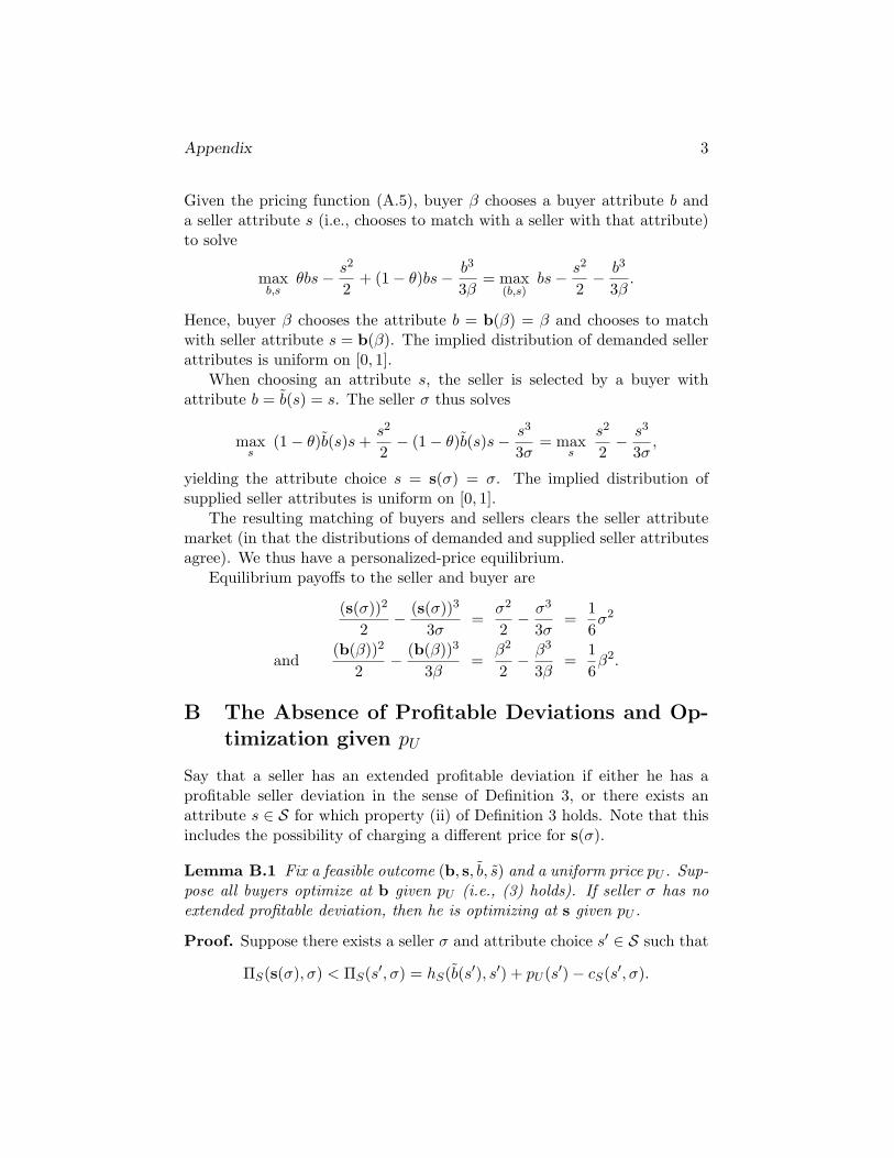
B The Absence of Profitable Deviations and Op-timization given pU

Say that a seller has an extended profitable deviation if either he has aprofitable seller deviation in the sense of Definition 3, or there exists anattribute s ∈ S for which property (ii) of Definition 3 holds. Note that thisincludes the possibility of charging a different price for s(σ).

Lemma B.1 Fix a feasible outcome (b, s, b, s) and a uniform price pU . Sup-pose all buyers optimize at b given pU (i.e., (3) holds). If seller σ has noextended profitable deviation, then he is optimizing at s given pU .

Proof. Suppose there exists a seller σ and attribute choice s′ ∈ S such that

ΠS(s(σ), σ) < ΠS(s′, σ) = hS(b(s′), s′) + pU (s′)− cS(s′, σ).

Appendix 4

Let ε = [ΠS(s′, σ)− ΠS(s(σ), σ)]/4 > 0. Then, there exists δ > 0 such thatfor all b ≥ b(s′)− δ,

hS(b, s′) + pU (s′)− cS(s′, σ) > ΠS(s(σ), σ) + 3ε. (B.1)

Denote by p′′ the price for an attribute s′′ that makes the buyer with at-tribute b(s′) indifferent between s′ (her equilibrium match) and s′′, i.e.,

hB(b(s′), s′′)− p′′ = hB(b(s′), s′)− pU (s′).

Choose s′′ > s′ sufficiently close to s′ so that∣∣hS(b, s′′)− cS(s′′, σ)− hS(b, s′) + cS(s′, σ)∣∣ < ε, ∀b ∈ B, (B.2)

holds and |p′′ − pU (s′)| < ε/2. From Assumption 1 (Supermodularity),

hB(b(s′)− δ, s′′)− p′′ < hB(b(s′)− δ, s′)− pU (s′).

For p < p′′ sufficiently close to p′′, we have p′′ − p > ε/2 and

hB(b(s′)− δ, s′′)− p < hB(b(s′)− δ, s′)− pU (s′).

Moreover the buyer with attribute b(s′) receives strictly higher payoff from(s′′, p) than from (s′, pU (s′))). Another application of Assumption 1 showsthat for all b ≤ b(s′)− δ,

hB(b, s′′)− p < hB(b, s′)− pU (s′).

From (3), for all b ∈ B,

hB(b, s′)− pU (s′) ≤ hB(b, s(b))− pU (s(b)),

and so no buyer with attribute b ≤ b(s′) − δ finds (s′′, p) attractive. Thus,the pair (s′′, p) is a profitable deviation for seller σ, since

hS(b(s′)− δ, s′′) + p− cS(s′′, σ) >hS(b(s′)− δ, s′) + p− cS(s′, σ)− ε≥ΠS(s(σ), σ) + 3ε+ (p− p′′) + (p′′ − pU (s′))− ε=ΠS(s(σ), σ) + ε,

where the first inequality follows from (B.2) and the second from (B.1).

Appendix 5

C Proof of Proposition 1: Efficient Uniform Pric-ing

Let (b, s, b, s, pP ) be an efficient personalized-price equilibrium (see SectionE; existence is established in Proposition E.1). We first show that the pricefunction can be altered so that the seller is indifferent over buyer attributes.In particular, (b, s, b, s, pP ) is a personalized-price equilibrium, where pP isthe personalized-price function given by

pP (b, s) = pP (b(s), s) + hS(b(s), s)− hS(b, s), ∀(b, s) ∈ B × S. (C.1)

Moreover, under pP , the seller is indifferent over all marketed buyer at-tributes.

To verify this, note that seller indifference is immediate, and it is thenimmediate that the seller is optimizing given pP . We then need show onlythat the buyer is optimizing given pU . Suppose (E.1) fails at some β. Then,for some (b, s) ∈ B × S and for sufficiently small ε > 0,

hB(b, s)− (pP (b, s) + ε)− cB(s, β) > ΠB(b(β), β).

Since no buyer has a profitable out-of-market deviation,

hS(b(s), s) + pP (b(s), s) ≥ hS(b, s) + pP (b, s) + ε.

But this, with (C.1), yields a contradiction.We now notice that if hS(b, s) does not depend on b, then neither does

pP , implying that (b, s, b, s, pU ) for pU (s) = pP (·, s) is a uniform-price equi-librium.

The constrained efficiency of uniform-price equilibria when the sellerpremuneration values do not depend on buyer attributes follows from theobservation that such equilibria are also personalized price equilibria andLemma E.2.

D Proof of Proposition 3: Existence of Equilib-rium.

The existence proof is involved and indirect. We would like to constructa game Γ whose equilibria induce uniform-price equilibria. However, theobvious such game Γ is itself difficult to handle, so we work with an approx-imating sequence of games Γn. We verify that each Γn has an equilibrium,

Appendix 6

take limits, and show that the limiting strategy profile induces a uniform-price equilibrium. Loosely, the n index allows us to accommodate (in thelimit) the possibility of jumps in the attribute-choice functions (precludedin game Γn).

D.1 Preliminaries

Let P = max{hB(b, s), hS(b, s)}. Then P is sufficiently large that no buyerwould be willing to purchase any seller attribute choice s ∈ [0, s] at a priceexceeding P , nor would any seller be willing to sell to a buyer b ∈ [0, b] atprice less than −P . We can thus limit prices to the interval [−P, P ].

Since buyer premuneration values are C2, there is a Lipschitz constant∆ such that for all ε > 0, s ∈ [0, s− ε], and b ∈ [0, b], we have hB(b, s+ ε)−hB(b, s) < ∆ε. As a result, given a choice between seller s and seller s+ε ata price higher by ∆ε, buyers would always choose the former. Equilibriumprices will thus never need to increase at a rate faster than ∆.

D.2 The game Γn

Each game Γn has three players, consisting of a buyer, a seller, and a price-setter.

D.2.1 Strategy spaces

We begin by defining the strategy spaces for Γn.The buyer chooses a pair of functions, (b, sB), where b : [0, 1] → [0, b]

specifies a buyer attribute choice and sB : [0, 1] → [0, s] a seller attributewith which to match, each as a function of the buyer’s type. We denotethe set of pairs of increasing functions (b, sB) normed by the sum of the L1

norms on the component functions by ΥB. In Γn, the buyer is restricted tothe subset of ΥB, denoted by Υn

B, of functions satisfying (D.1) and (D.2):

(β′ − β)/n ≤ b(β′)− b(β) ≤ n(β′ − β), ∀β < β′ ∈ [0, 1], (D.1)

and

(β′ − β)/n ≤ sB(β′)− sB(β) ≤ n(β′ − β), ∀β < β′ ∈ [0, 1]. (D.2)

The seller chooses an increasing function s, where s : [0, 1] → [0, s]specifies a seller attribute choice as a function of seller’s type. We denotethe set of increasing functions s endowed with the L1 norm by ΥS . In Γn,

Appendix 7

the seller is restricted to the subset of ΥS , denoted by ΥnS , of functions

satisfying (D.3),

(σ′ − σ)/n ≤ s(σ′)− s(σ) ≤ n(σ′ − σ), ∀σ < σ′ ∈ [0, 1]. (D.3)

The price-setter chooses an increasing function pU : [0, s] → [−P, P ]satisfying

pU (s′)− pU (s) < 2∆(s′ − s) (D.4)

for all s < s′ ∈ [0, s]. Denote the set of increasing functions pU satisfying(D.4), endowed with the sup norm, by ΥP (note that ΥP is not indexedby n). Every function in ΥP is continuous; indeed the collection ΥP isequicontinuous.

The set Υ ≡ ΥB × ΥS × ΥP , when normed by the sum of the threeconstituent norms, is a compact metric space.∗ It is immediate that Υn ≡ΥnB ×Υn

S ×ΥP is a closed subset of Υ, and so also compact.

D.2.2 Buyer and Price-Setter Payoffs

The buyer. The buyer’s payoff from (b, sB) ∈ ΥnB, when the price-setter

has chosen pU ∈ ΥP is∫(hB(b(β), sB(β))− pU (sB(β))− cB(b(β), β)) dβ. (D.5)

Note that the buyer’s payoff is independent of seller behavior.For any sB and s, define

FB(s) ≡ λ{β : sB(β) ≤ s}and FS(s) ≡ λ{σ : s(σ) ≤ s}.

∗It suffices for this conclusion to show that Υ is sequentially compact, since sequentialcompactness is equivalent to compactness for metric spaces (Dunford and Schwartz, 1988,p. 20). An argument analogous to that of Helly’s theorem (Billingsley, 1986, Theorem25.9) shows Υ is sequentially compact. In particular, given a sequence {(bm, smB , sm, pmU )},we can choose a subsequence along which each function converges at every rational valuein its domain to a limit {(b∞, s∞B , s∞, p∞U )}. Because each function in the sequence{(bm, smB , sm, pmU )} is increasing, so must be each limiting function {(b∞, s∞B , s∞, p∞U )}.This ensures convergence at every continuity point of the limit functions, and hence almosteverywhere for the functions bm, smB and sm and everywhere for the functions pmU )}, suffic-ing (for bounded functions) for L1 convergence in the former three cases and convergencein the sup norm in the latter.

Appendix 8

The price-setter. The price-setter’s payoff from pU ∈ ΥP , when thebuyer and seller have chosen (b, sB, s) ∈ Υn

B ×ΥnS is given by∫ s

0pU (s) (FB(s)− FS(s)) ds. (D.6)

Hence, the price-setter has an incentive to raise the price of seller attributechoices in excess demand and lower the price of seller attribute choices inexcess supply.

D.2.3 Seller Payoffs

The specification of the seller’s payoff is complicated by the need to incorpo-rate incentives arising from the possibility of profitable seller deviations toattribute choices outside S. Given an attribute choice s, price p, and pricefunction pU , set

B(s, p, pU ) ≡{b ∈ [0, b] : hB(b, s)− p ≥ max

s′∈[0,s]{hB(b, s′)− pU (s′)}

}.

(D.7)Hence, B(s, p, pU ) is the set of buyer attributes that find attribute s at pricep (weakly) more attractive than any attribute s′ ∈ [0, s] at price pU (s′). Notethat since the buyer is constrained in Γn to choose seller attributes so that(D.2) is satisfied, a maximizing buyer’s payoff from an attribute b (ignoringcosts) need not be given by maxs′∈[0,s]{hB(b, s′) − pU (s′)}. Note also thatfor all s and pU ∈ ΥP , since there is no a priori restriction on p, B(s, p, pU )is nonempty for low p (possibly requiring p < −P , e.g., if pU ≡ −P ), and itis empty if p > pU (s). Indeed, for sufficiently low p, B(s, p, pU ) = [0, b].

Lemma D.1 (1) If B(s, p, pU ) 6= ∅, then B(s, p, pU ) = [b1, b2] with b1 ≤ b2.(2) For fixed s and pU , let p(s, pU ) ≡ sup{p : B(s, p, pU ) 6= ∅} and

write [b1(p), b2(p)] for B(s, p, pU ) when p ≤ p(s, pU ). Denote the set ofdiscontinuity points in the domain of bj(p) by Dj(s, pU ) (j = 1, 2). The set{s : Dj(s, pU ) 6= ∅} has zero Lebesgue measure.

(3) Suppose {(s`, p`, p`U )}` is a sequence converging to (s, p, pU ) with ∅ 6=B(s`, p`, p`U ) ≡ [b`1, b

`2]. Then B(s, p, pU ) 6= ∅, and so B(s, p, pU ) = [b1, b2],

whereb1 ≤ lim inf` b`1 ≤ lim sup` b`2 ≤ b2. (D.8)

(4) Moreover,if p 6∈ Dj(s, pU ) ∪ {p(s, pU )}, then bj = lim` b`j.

Appendix 9

Proof. (1) Suppose b1, b2 ∈ B(s, p, pU ) with b1 < b2, and b 6∈ B(s, p, pU )for some b ∈ (b1, b2). Then there exists s ∈ [0, s] such that

hB(b, s)− p < hB(b, s)− pU (s).

If s > s, then Assumption 1 implies

hB(b2, s)− hB(b2, s) ≥ hB(b, s)− hB(b, s)> pU (s)− p,

contradicting b2 ∈ B(s, p, pU ). Similarly, s < s contradicts b1 ∈ B(s, p, pU ),and so s = s. But b2 ∈ B(s, p, pU ) then implies pU (s) ≥ p while b 6∈B(s, p, pU ) implies pU (s) < p, the final contradiction, and so b ∈ B(s, p, pU ).It is immediate that B(s, p, pU ) is closed.

(2) Since B(s, p′, pU ) ⊃ B(s, p, pU ) for p′ < p, b1(p) and b2(p) are mono-tonic functions of p, and so are continuous except at a countable number ofpoints. Moreover, we can apply the maximum theorem (since each of thefunctions in the maximum are continuous) to conclude that the right side ofthe inequality in (D.7) is continuous in b, and so b1 and b2 are left-continuousfunctions of p (as (D.7) features a weak inequality bounding p from above).

Suppose p ∈ D1(s, pU ), and let b+1 ≡ limp′↘p b1(p′). Since b1 is left-continuous, b1(p) < b+1 . Then for all b ∈ [b1(p), b+1 ],

hB(b, s)− p = maxs′∈[0,s]

hB(b, s′)− pU (s′). (D.9)

From the envelope theorem (Milgrom and Segal, 2002, Theorem 2), thisimplies for all b ∈ (b1(p), b+1 ),

∂hB(b, s)∂b

=∂hB(b, s′(b))

∂b,

where s′(b) ∈ arg maxs′∈[0,s] hB(b, s′) − pU (s′). Assumption 1 then impliess = s′(b) for all b ∈ (b1(p), b+1 ), and so p = pU (s).

Since b+1 ∈ B(s, pU (s), pU ), for all s′′ > s,

hB(b+1 , s′′)− hB(b+1 , s) ≤ pU (s′′)− pU (s)

so that∂hB(b+1 , s)

∂s≤ lim inf

s′′>s

pU (s′′)− pU (s)s′′ − s

.

On the other hand, for all s′ < s,

pU (s)− pU (s′) ≤ hB(b1(p), s)− hB(b1(p), s′),

Appendix 10

so that

lim sups′<s

pU (s)− pU (s′)s− s′

≤ ∂hB(b1(p), s)∂s

.

Consequently, since

∂hB(b1(p), s)∂s

<∂hB(b+1 , s)

∂s,

the price function pU cannot be differentiable at s. Finally, since pU is amonotonic function, it is differentiable almost everywhere (Billingsley, 1986,Theorem 31.2), and hence {s : D1(s, pU ) 6= ∅} has zero Lebesgue measure.A similar argument shows that {s : D2(s, pU ) 6= ∅} has zero Lebesguemeasure.

(3) Suppose {(s`, p`, p`U )}` is a sequence converging to (s, p, pU ), and let{b`} be a sequence of attributes with b` ∈ B(s`, p`, p`U ) for all `. By taking asubsequence if necessary, we can assume {b`} is a convergent sequence withlimit b. Since

hB(b`, s`)− p` ≥ maxs′∈[0,s]

{hB(b`, s′)− p`U (s′)}, ∀`,

taking limits gives

hB(b, s)− p ≥ maxs′∈[0,s]

{hB(b, s′)− pU (s′)},

and so b ∈ B(s, p, pU ). Hence, from part 2 of the lemma, B(s, p, pU ) =[b1, b2], and (D.8) the follows from taking sequences {b`} with limits lim inf` b`1and ≤ lim sup` b`2.

(4) Consider b2 and suppose p 6∈ D2(s, pU ) ∪ {p(s, pU )} (and so p <p(s, pU )). Hence, b2 = b+2 ≡ limp′↘p b2(p′). Consider b ∈ (b+1 , b2). For p′ > psufficiently close to p, we have b ∈ B(s, p′, pU ), and so

hB(b, s)− p > maxs′∈[0,s]

{hB(b, s′)− pU (s′)}.

Consequently, for ` sufficiently large,

hB(b, s`)− p` > maxs′∈[0,s]

{hB(b, s′)− pU (s′)},

i.e., b ∈ B(s`, p`, p`U ). This implies that b`2(p`) ≥ b, and hence lim inf b`2(p`) ≥b. Since this holds for all b ∈ (b+1 , b2) and lim sup` b`2 ≤ b2, we have lim` b

`2 =

b2. The argument for b1 is an obvious modification of this argument.

Appendix 11

Fix (s, p, pU ) and suppose λ({β : b(β) ∈ B(s, p, pU )}) > 0. Since bis strictly increasing and continuous, it then follows from Lemma D.1 thatb([0, 1]) ∩ B(s, p, pU ) = [b′1, b

′2] for some 0 ≤ b′1 < b′2 ≤ b. The payoff to the

seller from (s, p,b, pU ) is given by

H(s, p,b, pU ) ≡ hS(b′1, s) + p. (D.10)

This function depends upon pU and b through the dependence of b′1 onB(s, p, pU ) and b. For later reference, note that for fixed s, b, and pU ,the function H(s, p,b, pU ) is continuous from the left in p (since b satisfies(D.1) and both b1(p) and b2(p), defined just before Lemma D.1, are left-continuous).

We set

P (s,b, pU ) ≡ {p : λ ({β : b(β) ∈ B(s, p, pU )}) > 0} ,

and noting that this set is nonempty, define

H(s,b, pU ) ≡ max{

supp∈P (s,b,pU )H(s, p,b, pU ), hS(0, s) + pU (s)}.

(D.11)Notice that if p ∈ P (s,b, pU ) for all p < pU (s), then the first term in (D.11)will be the maximum.†

The seller’s payoff from s ∈ ΥnS when the buyer and price-setter have

chosen (b, sB, pU ) ∈ ΥnB ×ΥP is then∫ (H(s(σ),b, pU )− cS(s(σ), σ)

)dσ. (D.12)

Taking the maximum over supp∈P (s,b,pU )H(s, p,b, pU ) and hS(0, s) + pU (s)effectively assumes that the seller can always sell attribute choice s at theposted price pU (s), though perhaps only attracting buyer attribute choice0.

Note that the seller, when considering the payoff implications of alter-ing the attribute-choice function over an interval of seller types, can ignorethe seller types outside the interval, since feasibility of buyer responses isirrelevant (the comparison in B for buyer attributes is always to her payoffs,which is independent of seller behavior).

†It need not be true that for s ∈ sB([0, 1]), p ∈ P (s,b, pU ) for all p < pU (s). Moreover,we may have H(s,b, pU ) 6= hS(b(s−1

B (s)), s)+pU (s) (see the discussion just before LemmaD.1).

Appendix 12

D.3 Equilibrium in game Γn

Our next task is to show that each game Γn has a Nash equilibrium, and thatthe price-setter plays a pure strategy in any such equilibrium. To do this,we first note that the price-setter’s payoff is concave in pU (note that thebuyer’s and sellers’s payoffs need not be even quasiconcave). If the payofffunctions in game Γn are continuous, then Glicksberg’s fixed point theorem,applied to the game where we allow the buyer and seller to randomize, yieldsa Nash equilibrium in which the buyer and seller may randomize, but theprice-setter does not.

Lemma D.2 The buyer, price-setter and seller payoff functions given by(D.5),(D.6) and (D.12), are continuous functions of (b, sB, s, pU ) on Υn.

Proof. We first note that for increasing, bounded functions on a compactset, L1 convergence implies convergence almost everywhere.‡

Consider first the buyer. The functions b, sB, and pU are boundedfunctions on compact sets, and hence the absolute value of each of thesefunctions is dominated by an integrable function. The continuity of thebuyer’s payoff then follows immediately from Lebesgue’s dominated conver-gence theorem, if we can show that the convergence of b, pU , and sB inthe L1 norm (and hence almost everywhere) implies the convergence almosteverywhere of hB(b, sB), pU (sB), and cB(b(·), ·) (note that we are talkingabout sequences of functions within a given game Γn). The first and thethird of these follows from the continuity of hB and cB (from Assumptions1 and 3), while for the remaining case it suffices to note that the collectionΥP is equicontinuous.

Consider now the price-setter. Suppose s` converges in L1, and so almosteverywhere, to s. Then F `S converges weakly to FS (and so a.e.).§ Similarly,

‡Suppose {fn}n, with each fn increasing, converges in L1 norm to an increasing func-tion f without converging almost everywhere. Then since f is discontinuous on a set ofmeasure zero, there exists (for example) a continuity point x of f with lim sup fn(x) > f(x)(with the case lim inf fn(x) < f(x) analogous). The continuity of f at x then ensuresthat for some point y > x, some ε > 0, all z ∈ [x, y] and for infinitely many n, we havefn(z) ≥ fn(x) ≥ f(y)+ε ≥ f(z)+ε. This in turn ensures that

∫|fn(z)−f(z)|dz > (y−x)ε

infinitely often, precluding the L1 convergence of {fn}∞n=1 to f .§Fix ε > 0. By Egoroff’s theorem (Royden, 1988, p.73), s` converges uniformly to s

on a set E of measure at least 1 − ε. Suppose s is a continuity point of FS . There thenexists δ > 0 such that |FS(s) − FS(s′)| < ε for all |s − s′| ≤ δ. There exists `′ such that,for all σ ∈ E, for all ` > `′, |s`(σ)− s(σ)| < δ. Consequently, F `S(s) = λ{σ : s`(σ) ≤ s} ≤λ{σ : s(σ)−δ ≤ s}+ε = FS(s+δ)+ε and FS(s−δ)−ε ≤ F `S(s), and so |F `S(s)−FS(s)| < 2ε.Hence, F `S converges weakly to FS .

Appendix 13

if s`B converges in L1 to sB, then F `B converges a.e. to FB. Continuity for theprice-setter’s payoff then follows from arguments analogous to those appliedto the buyer, since we have convergence almost everywhere of pU [FB − FS ].

Finally, we turn to the seller, where the proof of continuity is moreinvolved. It suffices to argue that H(s,b, pU ) is continuous in (s,b, pU )for almost all s (since sB is irrelevant in the determination of the seller’spayoff and the continuity with respect to s is then obvious, at which pointanother appeal to Lebesgue’s dominated convergence theorem completes theargument).

Fix a sequence (s`,b`, p`U ) converging to some point (s, b, pU ). Since weneed continuity for only almost all s ∈ [0, s], we can assume D1(s, pU ) ∪D2(s, pU ) = ∅ (or, equivalently, that pU is differentiable at s, see the proofof Lemma D.1.2). We thus need only prove the following claim.

Claim 1 lim`→∞ H(s`,b`, p`U ) = H(s, b, pU ).

Proof. Since Hk(s,b, pU ) is the maximum of two terms, it suffices to showthat

lim`→∞

supp∈P (s`,b`,p`U )H(s`, p,b`, p`U ) = supp∈P (s,b,pU )

H(s, p, b, pU )

and lim`→∞

hS(0, s`) + p`U (s`) = hS(0, s) + pU (s).

The second is immediate from the continuity of hS and pU at s.We accordingly turn to the first. To conserve on notation, we define

supp∈P (s,b,pU )H(s, p,b, pU ) ≡ ¯H(s,b, pU ).We first show that

lim inf`→∞

¯H(s`,b`, p`U ) ≥ ¯H(s, b, pU ). (D.13)

For all ε > 0 there exists p ∈ P (s, b, pU ) such that

H(s, p, b, pU ) + ε/2 ≥ ¯H(s, b, pU ).

SinceH(s, p, b, pU ) is continuous from the left in p, there exists p′ 6∈ D1(s, pU )∪D2(s, pU ) ∪ {p(s, pU )} with p′ ≤ p satisfying

|H(s, p, b, pU )−H(s, p′, b, pU )| < ε/2,

and soH(s, p′, b, pU ) + ε ≥ ¯H(s, b, pU ).

Appendix 14

Since b satisfies (D.1), for sufficiently large `, p′ ∈ P (s`,b`, p`U ), and so(applying Lemma D.1.3)

lim`→∞

H(s`, p′,b`, p`U ) = H(s, p′, b, pU ).

Hence,lim inf`→∞

¯H(s`,b`, p`U ) + ε ≥ ¯H(s, b, pU ), ∀ε > 0,

yielding (D.13).We now argue that

¯H(s, b, pU ) ≥ lim sup`→∞

¯H(s`,b`, p`U ), (D.14)

which with (D.13) gives continuity.Fix ε > 0. For each `, there exists p` ∈ P (s`,b`, p`U ) such that

H(s`, p`,b`, p`U ) + ε ≥ ¯H(s`,b`, p`U ). (D.15)

Without loss of generality, we can assume {p`}` is a convergent sequence,with limit p. Suppose first that p ∈ P (s, b, pU ). If p 6= {p(s, pU )}, it isimmediate that

H(s, p, b, pU ) + ε ≥ lim sup`→∞

¯H(s`,b`, p`U ), (D.16)

which (since it holds for all ε) implies (D.14).Suppose now that p 6∈ P (s, b, pU ) or p = p(s, pU ). Since pU is differ-

entiable at s, there cannot be a nondegenerate interval of buyer attributesindifferent between (s, p) and the unconstrained optimal seller attribute un-der pU . This implies b([0, 1]) ∩B(s, p, pU ) = {b} for some b, and so

¯H(s, b, pU ) ≥ hS(b, s) + p.

From Lemma D.1.3,

lim`→∞

H(s`, p`,b`, p`U ) + ε = hS(b, s) + p+ ε,

and so (taking the lim sup of both sides of (D.15))

¯H(s, b, pU ) + ε ≥ lim sup`→∞

¯H(s`,b`, p`U ),

which (since it holds for all ε > 0) implies (D.14).

Appendix 15

Allowing the buyer and seller to choose mixed strategies then gives usa game whose best responses consist of closed, convex sets. As a result, wecan apply Glicksberg (1952) to conclude that we have a Nash equilibrium inwhich the price-setter plays a pure strategy, while the buyer and seller maymix:

Lemma D.3 The game Γn has a Nash Equilibrium, (ξnB, ξnS , p

nU ) ∈ ∆(ΥB)×

∆(ΥS)×ΥP .

D.4 The limit n→∞

We now examine the limit as n → ∞. In particular, let {(ξnB, ξnS , pnU )}n ⊂∆(ΥB) × ∆(ΥS) × ΥP be a sequence of Nash equilibria of the games Γn.Without loss of generality (since the relevant spaces are sequentially com-pact), we may assume that both the sequence of equilibria converges to somelimit (ξ∗B, ξ

∗S , p∗U ), and that players’ payoffs also converge.

We examine the limit (ξ∗B, ξ∗S , p∗U ). Intuitively, we would like to think of

this profile as the equilibrium of a “limit game.” However, the definitionof this limit game is not straightforward, since the definition of the seller’spayoffs in the game Γn relies on the strategies b, sB, and s having properties(such as strict monotonicity and continuity) that need not carry over to theirlimits. In establishing properties of (ξ∗B, ξ

∗S , p∗U ), we accordingly typically

begin our argument in the limit, and then pass back to the approximatingequilibrium profile (ξnB, ξ

nS , p

nU ) to obtain a contradiction. The latter step of

the argument is notationally cumbersome, and we do not always make theapproximation explicit.

Note that while the seller is best responding to ξnB in choosing s, thechoice of p implicit in (D.11) is made after (b, sB) is realized.

While the L1 topology does not distinguish between functions that agreealmost everywhere, it will be important for some of the later developmentsthat we make the selection indicated in the next lemma from the equivalenceclasses of functions that agree almost everywhere.

Lemma D.4 The limit profile (ξ∗B, ξ∗S , p∗U ) is pure, which we denote by

(b∗, s∗B, s∗, p∗U ). The limit functions can be (and subsequently are) taken

to be increasing, and the functions b∗, s∗B, and s∗ can be (and subsequentlyare) taken to be continuous from the left.

Proof. Consider the buyer (the case of the seller is analogous). Toward acontradiction, suppose the buyer’s strategy (ξ∗B, ξ

∗S) is not pure. Let ξ∗B,b and

ξ∗B,s denote the marginal distributions induced on buyer and seller attributes

Appendix 16

chosen by the buyer. Then define a pair of increasing functions b′ : [0, 1]→[0, b] and s′B : [0, 1]→ [0, s] by

b′(β) = inf{b : ξ∗B,b(b) ≥ β}and s′B(β) = inf{s : ξ∗B,s(s) ≥ β}.

These functions constitute pure strategies for the buyer giving the samedistribution of buyer and seller attributes chosen by the buyer. (For exam-ple, for any set [b, b] of buyer attributes with b > 0, ξ∗B,b[b, b] = β′′ − β′,where b′(β′′) = b and b′(β′) = b.) However, the b′ and s′B feature positiveassortativity between the buyer’s types and attribute choice, and betweenthe buyer’s and the seller’s attribute with which the buyer matches, whileξ∗B,b and ξ∗B,s, being mixed, do not. From Assumptions 1 and 3, this posi-tive assortativity increases the buyer’s payoff, and so the constructed purestrategy strictly increases the buyer’s payoff. It then follows from straight-forward continuity arguments that for sufficiently large n, i.e., for a game inwhich the slope requirements on the buyer’s strategy are sufficiently weakand the equilibrium profile (ξnB, ξ

nS , p

nU ) is sufficiently close to (ξ∗B, ξ

∗S , p∗U ),

there is a pure strategy sufficiently close to b′ and s′B giving the buyer apayoff higher than his supposed equilibrium payoff in Γn a contradiction.Hence, the buyer cannot mix.

The conclusion that each function is increasing is an implication of theobservation that if a sequence of increasing functions {fn} converges in L1

to a function f , then that function is increasing.

It is helpful to keep in mind the nature of convergence in ∆(ΥB) ×∆(ΥS) × ΥP . Recalling that ΥB, ΥS , are each endowed with the L1 normand ΥP with the sup norm, and the definition of the Prohorov metric(which metrizes weak convergence), (ξnB, ξ

nS , p

nU ) converges to the pure pro-

file (b∗, s∗B, s∗, p∗U ) if, and only if, the following holds: For all ε > 0 there

exists n′ such that for all n ≥ n′,

ξnB({

(b, sB) ∈ ΥnB :∫|b(β)− b∗(β)|dβ < ε,

∫|sB(β)− s∗B(β)|dβ < ε

})≥ 1− ε,

ξnS({

s ∈ ΥnS :∫|s(σ)− s∗(σ)|dσ < ε

})≥ 1− ε,

andsup |pnU (s)− p∗U (s)| < ε.

We next restate the nature of convergence in a more useful form:

Appendix 17

Lemma D.5 For all ε > 0, there exists a set Eε ⊂ [0, 1] with λ(Eε) ≥ 1−εand nε such that for all n ≥ nε,

ξnB ({(b, sB) ∈ ΥnB : |b(β)− b∗(β)| < ε, |sB(β)− s∗B(β)| < ε, ∀β ∈ Eε})

≥ 1− ε,

ξnS ({s ∈ ΥnS : |s(σ)− s∗(σ)| < ε, ∀σ ∈ Eε}) ≥ 1− ε,

and|pnU (s)− p∗U (s)| < ε, ∀s.

Moreover, the sets Eε are nested: Eε′ ⊂ Eε if ε < ε′.

Proof. Fix ε > 0. We prove that there is a set EεS with λ(EεS) > 1 − ε/3and an integer n′S such that

ξnS ({s ∈ ΥnS : |s(σ)− s∗(σ)| < ε, ∀σ ∈ EεS}) ≥ 1− ε (D.17)

for all n > n′S . The same argument implies a set EεB and integer n′B forthe function b∗, and a EεB and n′′B for the function s∗B.¶ The desired set isEε = EεS ∩ EεB ∩ EεB and integer is nε = max{n′S , n′B, n′′B}.

Let {σk} be an enumeration of the discontinuities of s∗. Since s∗ isbounded, there exists K such that the total size of the discontinuities over{σk}k>K is less than ε/6.

Fix L > 2 such that {(σk−2−kL, σk + 2−kL)}Kk=1 is pairwise disjoint and21−L < ε/6. Defining

EεS = [0, 1] \⋃k

(σk − 2−kL, σk + 2−kL)

yields a set of measure at least 1− ε/3.Let EKS be the set given by [0, 1] \ ∪Kk=1(σk − 2−kL, σk + 2−kL); clearly

EεS ⊂ EKS . The set EKS can be written as the disjoint union of closed intervals

¶More precisely, the sets can be chosen so that, for n > n′B ,

ξnB({(b, sB) ∈ ΥnB : |b(β)− b∗(β)| < ε, ∀β ∈ EεB}) ≥ 1− ε/2,

and, for n > n′′B ,

ξnB({(b, sB) ∈ ΥnB : |sB(β)− s∗B(β)| < ε, ∀β ∈ EεB}) ≥ 1− ε/2,

so that, for n > max{n′B , n′′B},

ξnB({(b, sB) ∈ ΥnB : |b(β)− b∗(β)| < ε, |sB(β)− s∗B(β)| < ε, ∀β ∈ EεB ∩ EεB}) ≥ 1− ε.

Appendix 18

Ik, k = 0, 1, . . . ,K. There exists an η > 0 such that for all k and for allσ, σ′ ∈ Ik, if |σ − σ′| < η then |s∗(σ)− s∗(σ′)| < ε/3.

Let {x`} ⊂ Ik be an η-grid of Ik, i.e., x`+1 − η < x` < x`+1 for all `.Consider an increasing function s satisfying

∫|s− s∗| < εη/3. We claim

that for all σ ∈ EKS (and so for all σ ∈ EεS), |s−s∗| < ε. Observe that (D.17)then follows, since n′S can be chosen so that ξnS

({s ∈ Υn

S :∫|s− s∗| < εη/3

})≥

1− ε holds for all n > n′S .The claim follows from two observations:

1. |s(x`) − s∗(x`)| < 2ε/3: Suppose s(x`) ≥ s∗(x`) + 2ε/3 (the otherpossibility is handled mutatis mutandis). Then, for all σ ∈ (x`, x`+1),

s(σ) ≥ s(x`) ≥ s∗(x`) + 2ε/3 > s∗(σ) + ε/3.

But this is impossible, since it would imply∫|s− s∗| > εη/3.

2. For all ` and all σ ∈ (x`, x`+1), |s(σ) − s∗(σ)| < ε: Suppose s(σ) ≥s∗(σ) + ε (the other possibility is handled mutatis mutandis). Then,

s(x`+1) ≥ s(σ) ≥ s∗(σ) + ε ≥ s∗(x`+1) + 2ε/3,

contradicting the previous observation.

The last assertion of Lemma D.5 is immediate from the definition of EεS .

Lemma D.6 The profile (b∗, s∗B, s∗, p∗U ) balances the market, i.e., F ∗B(s) =

F ∗S(s) for all s. Hence, s∗B(x) = s∗(x) for almost all x ∈ [0, 1].

Proof. Since F ∗B and F ∗S are continuous from the right, it suffices to showthat they agree almost everywhere. We first argue that F ∗B(s) − F ∗S(s) ≤ 0almost everywhere. Suppose this is not the case, so there exists s < s withF ∗B(s) − F ∗S(s) = ε > 0 and with s a continuity point of F ∗B − F ∗S . Thenthere exists s1 and s2 with s ∈ (s1, s2), F ∗B(s) − F ∗S(s) ≥ ε/2 on [s1, s2],and either s1 = 0 or, for every η > 0, there is a value sη ∈ [s1 − η, s1) withF ∗B(sη) − F ∗S(sη) < ε/2 (note that F ∗B(sη) − F ∗S(sη) may be negative, andso is bounded below by −1). We consider the case in which s1 > 0 andp∗U (s1) < p∗U (s2), with the remaining cases a straightforward simplification.

Since F ∗B(s) − F ∗S(s) > 0 on [s1, s2], for fixed p∗U (s1) and p∗U (s2), theprice-setter must be setting prices as large as possible on this interval. Ifnot, there is a price function pU ∈ ΥP with pU (s) ≥ p∗U (s) for all s and

Appendix 19

pU (s) > p∗U (s) for some s yielding strictly higher payoffs to the price-setterthan p∗U in Γn for sufficiently large n, when the buyer and seller choose(ξnB, ξ

nS). But this contradicts the equilibrium property of (ξnB, ξ

nS , p

nU ).

Hence, there exists s′ ∈ [s1, s2] such that dp∗U (s)/ds = 2∆ on (s1, s′) and

p∗U (s) = p∗U (s2) for s ∈ [s′, s2]. That is, prices increase at the maximumrate possible until hitting p∗U (s2) (with s′ = s2 possible, but since p∗U (s1) <p∗U (s2), we have s1 < s′). Consequently, sB([0, 1]) ∩ [s1, s2] ⊂ {s1, s2}, i.e.,buyers demand only seller attribute choices s1 and s2 from this interval.(Since all seller attribute choices in [s′, s2] command the same price, buyersdemand only attribute choice s2 from this set, while the price of a sellerattribute choice increases sufficiently quickly on [s1, s

′] that from this setbuyers demand only s1.)

Since for every η > 0, there exists sη ∈ [s1−η, s1) with F ∗B(sη)−F ∗S(sη) <ε/2 and yet F ∗B(s1)−F ∗S(s1) ≥ ε, the buyer must choose attributes arbitrarilyclose to s1 for some buyer types. This implies that there is a range of sellerattributes just below s1 with prices that are not too low, that is, there existsη′ > 0 such that

p∗U (s) > p∗U (s1)−∆(s1 − s)

for all s ∈ [s1 − η′, s1). Consider now the price function pηU ∈ ΥP given by

pηU (s) ≡

p∗U (s), if s ≥ s′,min{p∗U (s1 − η) + 2∆(s− s1 + η), p∗U (s′)}, if s ∈ (s1 − η, s′),p∗U (s), if s ≤ s1 − η,

and note that p0U = p∗U . Since pηU ≥ p∗U , the price-setter’s payoff from

choosing pηU ∈ ΥP less the payoff from p∗U is bounded below by

−∫ s1

s1−η

(pηU (s)− p∗U (s)

)ds+

∫ s′

s1

(pηU (s)− p∗U (s)

)ε/2 ds. (D.18)

For η < η′ and s ∈ (s1 − η, s1),

pηU (s)− p∗U (s) ≤ p∗U (s1 − η) + 2∆(s− s1 + η)− p∗U (s1) + ∆(s1 − s)= p∗U (s1 − η)− p∗U (s1)−∆(s1 − s) + 2∆η≤ 2∆η.

Moreover, for s ∈ (s1, s1 + (s′−s1)/2), if η is sufficiently close to 0, we have

Appendix 20

pηU (s) < p∗U (s′) and so

pηU (s)− p∗U (s) = p∗U (s1 − η) + 2∆(s− s1 + η)− p∗U (s)≥ p∗U (s1)−∆η + 2∆(s− s1 + η)− p∗U (s)= p∗U (s1)−∆η + 2∆(s− s1 + η)− p∗U (s1)− 2∆(s− s1)= ∆η.

Since pηU (s) ≥ p∗U (s) for all s, the expression in (D.18) is bounded below by

−∫ s1

s1−η2∆η ds+

∫ s1+(s′−s1)/2

s1

∆ηε/2 ds,

which is clearly positive for sufficiently small η. Since the lower bound isstrictly positive, the price-setter has a profitable deviation (in Γn for largen), a contradiction.

We conclude that F ∗B(s) − F ∗S(s) ≤ 0 for almost all s. It remains toargue that it is not negative on a set of positive measure. Suppose it is.Then there must exist a seller characteristic s > 0 such that pU (s) = −Pfor s < s, F ∗B(s) − F ∗S(s) < 0 for a positive-measure subset of [0, s], andF ∗B(s) − F ∗S(s) = 0 for almost all s > s. But then no seller would chooseattributes in [0, s), a contradiction.

We now seek a characterization of the seller’s payoffs. Intuitively, wewould like to use Lemma D.6 and the monotonicity of b∗ and s∗B to concludethat there is positive assortative matching, and indeed that a seller of typeσ matches with a buyer of type β = σ. However, these properties may nothold if b∗ and s∗B are not strictly increasing. Moreover, even if we had sucha matching, the specification of the seller’s payoffs given by (D.12) leavesopen the possibility that the (gross) payoff to a seller of type σ choosingattribute s may not be given by hS(b(s), s) + pU (s). Hence, the buyers thatsellers are implicitly choosing in their payoff calculations may not duplicatethose whose seller choices balance the market.

Our first step in addressing these issues is to show that the buyer’slimiting attribute-choice function is indeed strictly increasing. Intuitively, ifa positive measure of buyer types choose the same attribute, by having somehigher types in the pool choose a slightly higher attribute, and some lowertypes choose a slightly lower attribute, we can keep the average attributeunchanged, while saving costs (from Assumption 3).

Lemma D.7 The function b∗ is strictly increasing when nonzero.

Appendix 21

Proof. By construction, b∗ is weakly increasing. We show that β′′ > β′

and b∗(β′) > 0 imply b∗(β′′) > b∗(β′). Suppose to the contrary that b =b∗(β) > 0 for two distinct values of β.

Define β1 ≡ inf{β : b∗(β) = b}, β2 ≡ sup{β : b∗(β) = b}, and β =(β1 + β2)/2. We assume 0 < β1 and β2 < 1 (if equality holds in either case,then the argument is modified in the obvious manner). We now define anew attribute-choice function (as a function of a parameter η > 0) that isstrictly increasing on a neighborhood of [β1, β2] and agrees with b∗ outsidethat neighborhood. First, define

βη1 = inf{β ≤ β1 : b∗(β) ≥ b+ η(β − β)}and βη2 = sup{β ≥ β2 : b∗(β) ≤ b+ η(β − β)}.

Note that as η → 0, βηj → βj for j = 1, 2. Finally, define

bη(β) ≡

b∗(β), if β > βη2,

b+ η(β − β), if β ∈ [βη1, βη2],

b∗(β), if β < βη1.

The difference in payoffs to the buyer under bη and under b∗ is given by∫ βη2

βη1

hB(bη(β), s∗B(β))−hB(b∗(β), s∗B(β))− [cB(bη(β), β)−cB(b∗(β), β)] dβ.

(D.19)Now,∫ β2

β1

[cB(bη(β),β)− cB(b∗(β), β)] dβ

=∫ β2

β1

[∂cB(b, β)

∂bη(β − β) + o(η)

]dβ

=η∫ (β2−β1)/2

0

[∂cB(b, β + x)

∂b− ∂cB(b, β − x)

∂b

]x dx+ o(η).

From Assumption 3, the integrand is strictly negative, and so the integralis strictly negative and independent of η. Since s∗B is increasing, a similarargument applied to the difference in the premuneration values shows that∫ β2

β1

hB(bη(β), s∗B(β))−hB(b∗(β), s∗B(β))−[cB(bη(β), β)−cB(b∗(β), β)] dβ

≥ η∫ (β2−β1)/2

0

[∂cB(b, β − x)

∂b− ∂cB(b, β + x)

∂b

]x dβ + o(η).

Appendix 22

It remains to argue that the contribution to (D.19) from the intervals [βη1, β1)and (β2, β

η2] is of order o(η). But this is immediate, since |bη(β)−b∗(β)| ≤ η

and βηj → βj as η → 0 (for j = 1, 2). Hence, for η > 0 sufficiently small,bη gives the buyer a strictly higher payoff under (D.5) than b∗. But, thenby a now familiar argument, the buyer has a profitable deviation in Γn

for sufficiently large n, a contradiction. So b∗ is strictly increasing whennonzero.

We next show that the seller’s payoffs converge to the payoff one wouldexpect the seller to receive by matching with his corresponding buyer type.

Lemma D.8 For almost all σ satisfying b∗(σ) > 0,

limn

∫H(s(σ),b, pnU )− cS(s(σ), σ)dξn

= hS(b∗(σ)), s∗(σ)) + p∗U (s∗(σ))− cS(s∗(σ), σ).

The functions s and b on the left side of this expression are strategies in thegame Γn, and are the objects over which the equilibrium ξn mixes.

Proof. Suppose the claim is false. Then, since the limit exists, there existsn′′ and η > 0 such that for all σ in a set G of sellers of measure at least ηwhose “matched” buyers choose positive attributes (i.e., b∗(σ) > 0), for alln > n′′, ∫

H(s(σ),b, pnU )− cS(s(σ), σ)dξn

is at least η distant from

hS(b∗(σ), s∗(σ)) + p∗U (s∗(σ))− cS(s∗(σ), σ).

Since G has positive measure, we may assume that every index in G isa continuity point of the limit functions (b∗, s∗B, s

∗).For any ε > 0, let Eε ⊂ [0, 1] be the set from Lemma D.5 satisfying

λ(Eε) ≥ 1− ε.Fix an index σ′ ∈ G ∩ Eε′ for some ε′ > 0 (since Eε is monotonic in ε,

σ′ ∈ G ∩ Eε for all smaller ε). Since b∗ is strictly increasing, without lossof generality, we may assume that, for all ζ > 0, there is a positive measureset of buyers with b∗(β) ∈ (b∗(σ′) − ζ,b∗(σ′)). Indeed, a positive measureset of buyers in Eε does so for all ε sufficiently small. Formally,

∀ζ > 0 ∃ε′′ ∀ε < ε′′, λ{β ∈ Eε : b∗(β) ∈ (b∗(σ′)− ζ,b∗(σ′))} > 0. (D.20)

Appendix 23

Consider some ε < ε′ and suppose n > max{nε, n′′}, where nε is fromLemma D.5. Let (b, sB, s) ∈ Υn

B × ΥnS be a triple of functions with the

property that |b(β) − b∗(β)| < ε and |sB(β) − s∗B(β)| < ε for all β ∈ Eε,and |s(σ) − s∗(σ)| < ε for all σ ∈ Eε. (Recall that, from Lemma D.5, ξn

assigns high probability to such functions for large n.)By Lemma D.6, s∗ and s∗B are equal almost surely, so without loss of

generality, we may assume that s∗(x) = s∗B(x) for all x ∈ E.Observe first that if the max in (D.11) is achieved by hS(0, s(σ)) +

pnU (s(σ)), then

H(s(σ),b, pnU )− cS(s(σ), σ) = hS(0, s(σ)) + pnU (s(σ))− cS(s(σ), σ)≤ hS(b(σ), s(σ)) + pnU (s(σ))− cS(s(σ), σ).

We claim that, for sufficiently small ε > 0, the set P (s(σ),b, pnU ) containsall p < pnU (s(σ)). This follows from (D.20) and the observation that buyersin Eε receive a payoff (ignoring costs) arbitrarily close to hB(b∗(β), s∗(β))−p∗U (s∗(β)).

Consequently, for p sufficiently close to pnU (s(σ)), single crossing (As-sumption 1) implies that a buyer β with attribute satisfying b∗(β) < b∗(σ)will not be attracted (for sufficiently large n). This implies that

supp∈P (s(σ),b,pnU )

H(s(σ), p,b, pnU ) = hS(b(σ), s(σ)) + pnU (s(σ)).

By choosing ε small (or, equivalently, n large), the right side can be madearbitrarily close to

hS(b1(s′), s′) + p∗U (s′) = hS(b1(s∗(σ)), s∗(σ)) + p∗U (s∗(σ)).

Hence, the max in (D.11) is achieved by the first term, and we have acontradiction.

With this payoff characterization in hand, we can show that seller at-tribute choices are strictly increasing in types (when positive), as are thetypes of sellers with whom buyers attempt to match.

Lemma D.9 The functions s∗B and s∗ are strictly increasing on {β : b∗(β) >0}.

Proof. From Lemma D.6, s∗B(x) = s∗(x) for almost all x ∈ [0, 1], and so itsuffices to prove the result for s∗. Suppose to the contrary there is a strictlypositive constant s and associated maximal nondegenerate interval (σ1, σ2)

Appendix 24

with s∗(σ) = s and b∗(σ) > 0 for all σ ∈ (σ1, σ2). From Lemma D.6, wealso have s∗B(β) = s for all β ∈ (σ1, σ2).

Define b1 ≡ limβ↓σ1 b∗(β) and b2 ≡ limβ↑σ2 b∗(β).Define σ(η) ≡ inf{σ : s∗(σ) ≥ s+ η}, and notice that limη→0 σ(η) = σ2.

The seller attribute-choice function s′ given by

s′(s) ={

s∗(σ), if σ 6∈ (σ1, σ(η)),s+ η, if σ ∈ (σ1, σ(η)),

is weakly increasing. Consider the price p > p∗U (s) for attribute s + ηsatisfying

p = sup{p : B(s+ η, p, p∗U ) 6= ∅}.(This is p(s+ η, p, p∗U ) from Lemma D.1(1).) The price p is at least as highas the value p′ satisfying hB(b2, s)− pU (s) = hB(b2, s+ η)− p′. At the pricep for attribute choice s + η, the seller ensures that attribute choice s + ηis chosen by a buyer at least as high as b2 (the single-crossing conditionon buyer premuneration values ensures that no lower attribute buyers willchoose s + η). From Lemma D.8, we have then have that the switch toattribute-choice function s′ increases the seller’s payoff by at least∫ σ2

σ1

(hS(b2, s+ η) + p) dσ −∫ σ2

σ1

(hS(b1, s) + p∗U (s)) dσ

−∫ σ(η)

σ1

(cs(s+ η, σ)− cS(s∗(σ), σ)dσ

> (σ2 − σ1)[hS(b2, s+ η)− hS(b1, s]− (σ(η)− σ1)[cS(s+ η, σ1)− cS(s, σ1)].

The first term after the inequality is bounded away from zero as η approacheszero, while the second approaches zero as does η, ensuring that there is someη > 0 for which the payoff difference is positive. Intuitively, each seller inthe interval (σ1, σ2) experiences a discontinuous increase in expected buyer(at a higher price) when increasing her attribute choice, while sellers in theinterval (σ2, σ(η)) experience a continuous increase in cost. The attribute-choice function s′ increases the seller’s payoff for sufficiently small η, yieldingthe result.

The limiting mass of buyers and seller choosing zero attributes are equal:

Lemma D.10

λ({σ : s∗(σ) = 0}) = λ({β : b∗(β) = 0}).

Appendix 25

Proof. First, suppose λ({β : b∗(β) = 0}) > λ({σ : s∗(σ) = 0}). Thenbecause s∗B = s∗ almost everywhere, there exists a positive mass of buyersfor whom b∗(β) = 0 and s∗B(β) > 0. By Assumption 2, hB(0, s) is inde-pendent of s, and so, since p∗U is strictly increasing, the buyers choosingb = 0 can increase their payoff by choosing s = 0. The buyer’s equilibriumstrategy must then be suboptimal in the game Γn for sufficiently large n, acontradiction.

Now, suppose λ({β : b∗(β) = 0}) < λ({σ : s∗(σ) = 0}). Then thereexists a positive mass of buyers for whom b∗(β) > 0 and s∗B(β) = 0. ByLemma D.6, there is then a positive mass of buyers choosing a zero sellerattribute and positive buyer attribute. Since hB(b, 0) is independent of b(Assumption 2) and cB(b, β) is strictly increasing in b, such buyers can in-crease their payoff by choosing b = 0. The buyer’s equilibrium strategy mustthen be suboptimal in the game Γn for sufficiently large n, a contradiction.

We now turn to feasible matchings. For b ∈ [0,b∗(1)] and s ∈ [0, s∗(1)],we define

b∗(s) ≡

{b∗((s∗)−1(s)), s ∈ s∗([0, 1]), s > 0,max {0, supb∈B{b < b∗(inf {σ : s∗ (σ) > s})}} , otherwise,

and

s∗(b) ≡

{s∗((b∗)−1(b)), b ∈ b∗([0, 1]), b > 0,max {0, sups∈S{s < s∗(inf{β : b∗(β) > b})}} , otherwise.

The maximum in the specification of b∗ (with s∗ similar) ensures that b∗ iswell defined when s∗ is continuous at inf{σ|s∗(σ) > 0} (in which case, thesupremum is taken over the empty set and so has value −∞).

Lemma D.11 The pair (b∗, s∗) is a feasible matching. In addition, for allvalues b > 0 and s > 0, we have

s∗(b) = s∗((b∗)−1(b))

where

(b∗)−1(b) =

{inf{β : b∗(β) > b}, for b ≤ b∗(1),1, for b > b∗(1),

andb∗(s) = b∗((s∗)−1(s)),

Appendix 26

where

(s∗)−1(s) =

{inf{σ : s∗(σ) > s}, for s ≤ s∗(1),1, for s > s∗(1).

Proof. From Lemma D.10, we can assume that b∗ and s∗ share a commonset [0, x] on which they are zero. It is then immediate that (b∗, s∗) is afeasible matching.

The final two statements follow immediately from the left continuity ofthe attribute-choice functions (see Lemma D.4) and the definitions of s∗ andb∗.

Finally, we show that the seller’s payoff satisfies an optimality condition.

Lemma D.12 For almost all σ,

limn

∫H(s(σ),b, pnU )− cS(s(σ), σ)dξn

= hS(b∗(σ), s∗(σ)) + p∗U (s∗(σ))− cS(s∗(σ), σ)

= maxs∈S

hS(b∗(s), s) + p∗U (s)− cS(s, σ).

Proof. The first inequality duplicates Lemma D.8.Single-crossing (Assumption 3) implies that the attribute choices maxi-

mizing hS(b∗(s), s)+p∗U (s)−cS(s, σ) are increasing in σ, and so if the secondequality fails, in games Γn for sufficiently large n, the seller has a profitabledeviation.

D.5 Uniform-Price Equilibria

We finally argue that the profile (b∗, s∗, b∗, s∗, p∗U ) induces a uniform-priceequilibrium of the matching market with identical attribute choices andmatching function (but perhaps a vertical shift in the price function).

The first task is to show that equilibrium payoffs are nonnegative, sothat agents would not prefer to be out of the market. Suppose {ξnB, ξnS , pnU}nis the sequence whose limit induces (b∗, s∗B, b

∗, s∗, p∗U ). We have

hB(0, 0)− p∗U (0) = hB(0, 0)− p∗U (0)− cB(0, β)≤ hB(b(β), s∗(b∗(β)))− p∗U (s∗(b∗(β)))− cB(b(β), β) (D.21)

Appendix 27

and

hS(0, 0) + p∗U (0) = hS(0, 0) + p∗U (0)− cS(0, σ)

≤ hS(b∗(s(σ)), s(σ)) + p∗U (s(σ))− cS(s(σ), σ). (D.22)

Letκ∗ ≡ hB(0, 0)− p∗U (0) ≥ −hS(0, 0)− p∗U (0)

(where the inequality follows from Assumption 2) and replace the pricefunction p∗U with p∗U +κ∗. Both ξnB and ξnS remain best responses given pricepnU + κ∗ and markets still clear in the limit of n→∞. Moreover, replacingp∗U with p∗U + κ∗ in (D.21)–(D.22) gives nonnegative payoffs.

It is immediate from the formulation of the buyer’s payoffs in the gameand from Lemma D.12 that almost all buyers and sellers are optimizinggiven p∗U .

It remains to consider deviations by a seller of type σ to a value s notchosen by any seller under s∗. If there is a profitable such deviation forseller σ, then there is a price p such that B(s, p, p∗U ) is nonempty and for allb ∈ B(s, p, p∗U ),

ΠS(s∗(σ), σ) < hS(b, s) + p− cS(s, σ).

But then for all sufficiently large n, B(s, p′, pnU ) is again nonempty for p′

less than but close to p, contradicting the fact that ΠS(s∗(σ), σ) is close to∫H(s(σ),b, pnU )− cS(s(σ), σ) dξn.

D.6 Nontriviality

Partial nontriviality. We now show that under (14), the profile (b∗, s∗, b∗, s∗, p∗U )is nontrivial. If the equilibrium is trivial, b∗ and s∗ are identically zero, sothat there is no agent for whom it is profitable to trade at price pU , andhence for all (b, s) ∈ (0, b]× (0, s],

hS(0, s) + pU (s)− cS(s, 1) ≤ 0and hB(b, s)− pU (s)− cB(b, 1) ≤ 0,

where we focus on agents β = 1 = σ since they are the most likely to wantto trade. Notice that we are using here the maximum that appears in thebuilding block (D.11) for the specification of the seller’s payoff, and whicheffectively allows the seller to sell any attribute choice s ∈ [0, s] at price

Appendix 28

pU (s), assuming in the process that he can attract at least a zero-attributebuyer. For these two inequalities to hold, it must be that

hB(b, s) + hS(0, s) ≤ cB(b, 1) + cS(s, 1),

contradicting (14).Full nontriviality. We now assume (15) holds. Suppose that there is

an interval of seller types [0, σ′] with σ′ > 0 who choose zero attributes. ByLemma D.9, we then have b∗(β) = 0 for all β ∈ [0, σ′]. If neither agent oftype φ ∈ (0, β′) chooses a strictly positive attribute, it must be that

hS(0, s) + pU (s)− cS(s, φ) ≤ 0and hB(b, s)− pU (s)− cB(b, φ) ≤ 0,

where (b, s) are a pair of attributes satisfying (15). But summing these twoinequalities yields an inequality contradicting (15).

E Personalized Pricing

E.1 Prices

A personalized-price function is a function pP : B × S → R; where pP (b, s)is the (possibly negative) price that seller with attribute choice s ∈ S re-ceives when selling to a buyer with attribute choice b ∈ B. We emphasizethat a personalized-price function prices only matches between marketedattributes.

E.2 Equilibrium

Given a feasible outcome (b, s, b, s) and a personalized price pP , the payoffsto a buyer β who chooses b ∈ B and to a seller σ who chooses s ∈ S aregiven by

ΠB(b, β) ≡ hB(b, s(b))− pP (b, s(b))− cB(b, β)

and ΠS(s, σ) ≡ hS(b(s), s) + pP (b(s), s)− cS(s, σ).

The specification of equilibrium begins with appropriate modificationsof the notions of buyer and seller optimization given pU (i.e., (3) and (4)):

Appendix 29

Definition E.1 Given a feasible outcome (b, s, b, s), buyer β is optimizingat b given pP if

(b(β), s(b(β))) ∈ arg max(b,s)∈B×S

hB(b, s)− pP (b, s)− cB(b, β). (E.1)

Seller σ is optimizing at s given pP if

(b(s(σ)), s(σ)) ∈ arg max(b,s)∈B×S

hS(b, s) + pP (b, s)− cS(s, σ). (E.2)

Since the personalized-price function pP prices only pairs of marketedattributes, the stipulation that a seller optimize given pP says nothing aboutwhat might happen if this seller chooses an attribute s 6∈ S. We require thatno seller can choose an attribute s 6∈ S, find a target buyer attribute b ∈ Bwith whom to match, and find a way to split the resulting surplus so thatthe seller and target buyer are both better off than in equilibrium:‖

Definition E.2 Given (b, s, b, s, pP ), there is a profitable seller deviationif there exists a seller σ such that either ( i) ΠS(s(σ), σ) < 0 or ( ii) thereexist an unmarketed seller attribute choice s 6∈ S, a marketed buyer attributeb ∈ B, and a price p ∈ R such that

hB(b, s(b))− pP (b, s(b)) < hB(b, s)− p (E.3)and ΠS(s(σ), σ) < hS(b, s) + p− cS(s, σ). (E.4)

The definition of a buyer’s profitable deviation is similar:

Definition E.3 Given (b, s, b, s, pP ), there is a profitable buyer deviationif there exists a buyer β such that either ( i) ΠB(b(β), β) < 0 or ( ii) thereexist an unmarketed buyer attribute choice b 6∈ B, a marketed seller attributes ∈ S, and a price p ∈ R such that

ΠB(b(β), β) < hB(b, s)− p− cB(b, β)

and hS(b(s), s) + pP (b(s), s) < hS(b, s) + p.

Definition E.4 A feasible outcome (b, s, b, s) and a personalized-price func-tion pP constitute a personalized-price equilibrium if all buyers and sellersare optimizing given pP and no buyer or seller has a profitable deviation.‖Similar to footnote 6, Definitions E.2 and E.3 can be extended to cover deviations to

any seller attribute, as well as to prices that differ from the personalized-price function.See Mailath, Postlewaite, and Samuelson (2010) for details.

Appendix 30

Remark E.1 (Premuneration Values) Since personalized prices can com-pensate for any alterations of the division of v(b, s), the decompositionof the surplus v(b, s) between the buyer’s and seller’s premuneration val-ues plays no role in the efficiency of a personalized-price equilibrium out-come. In particular, it is a straightforward calculation that if (b, s, b, s, pP )is a personalized-price equilibrium with premuneration values hB(b, s) andhS(b, s), then (b, s, b, s, p′P ) is a personalized-price equilibrium with premu-neration values h′B(b, s) and h′S(b, s), where

p′P (b, s) = pP (b, s) + h′B(b, s)− hB(b, s) = pP (b, s) + hS(b, s)− h′S(b, s).

�

Remark E.2 (Ex Post Contracting Equilibrium) Cole, Mailath, andPostlewaite (2001) study continua of buyers and sellers who first simultane-ously choose attributes (as here), and then match and bargain to divide theresulting surplus v(b, s), with the matching/bargaining stage being modeledas a cooperative game (more specifically, an assignment game). An ex postcontracting equilibrium in Cole, Mailath, and Postlewaite (2001) is a Nashequilibrium of the noncooperative attribute-choice game, where the payoffsfrom the attribute choices are determined by stable (equivalently, core) allo-cations in the induced assignment game.∗∗ The set of outcomes and impliedpayoffs are essentially the same under the two notions (modulo some techni-cal differences). In particular, if all buyers and sellers are optimizing in themarket given pP , then no buyer-seller pair with attributes (b, s) ∈ B×S canblock the equilibrium. Moreover, a seller σ has a profitable out-of-marketdeviation if and only if there is a blocking pair consisting of that seller (withsome attribute s) and some buyer with an attribute b ∈ B. An analogouscomment applies to buyers. �

E.3 Efficiency

Lemma E.1 In any personalized-price equilibrium (b, s, b, s, pP ), b and sare strictly increasing for strictly positive attributes.

Proof. We consider only b (since s is almost identical). Suppose b is notstrictly increasing. Since b is one-to-one on s((σ, 1]) (see Definition 1 and its∗∗Consequently, matching is over buyers and sellers, not attributes as here. This differ-

ence results in some technical complications.

Appendix 31

following comment), there exists 0 < s1 < s2 with b1 ≡ b(s1) > b(s2) ≡ b2.From (E.1) for the buyer choosing b1 and from (E.2) for the seller choosings2, we have

hB(b1, s1)− pP (b1, s1) ≥ hB(b1, s2)− pP (b1, s2)and hS(b2, s2) + pP (b2, s2) ≥ hS(b1, s2) + pP (b1, s2),

and so

hB(b1, s1) + hS(b2, s2)− pP (b1, s1) + pP (b2, s2) ≥ v(b1, s2).

Adding this to the analogous inequality obtained from (E.1) for the buyerchoosing b2 and from (E.2) for the seller choosing s1, we obtain

v(b1, s1) + v(b2, s2) ≥ v(b1, s2) + v(b2, s1).

But Assumption 1 requires the reverse (strict) inequality, a contradiction.

From Lemma E.1, matching in a personalized-price equilibrium is pos-itively assortative in attributes. Since the attribute-choice functions arestrictly increasing in index when positive, we can accordingly define the exante surplus for buyer and seller types β = σ = φ ∈ [0, 1] as

W (b, s, φ) ≡ hB(b, s) + hS(b, s)− cB(b, φ)− cS(s, φ)= v(b, s)− cB(b, φ)− cS(s, φ).

An efficient choice of attributes maximizes W (b, s, φ) for (almost) all φ.Personalized-price equilibrium outcomes are constrained efficient in the

sense that no matched pair of agents can increase its net surplus withoutboth agents deviating to attribute choices outside the sets of marketed at-tributes B and S:††

Lemma E.2 Suppose (b, s, b, s, pP ) is a personalized-price equilibrium. Then,for all φ ∈ [0, 1], b ∈ B, s ∈ S and all b′ and s′,

W (b, s′, φ) ≤W (b(φ), s(φ), φ)and W (b′, s, φ) ≤W (b(φ), s(φ), φ).

††This is essentially Cole, Mailath, and Postlewaite (2001, Lemma 2), which describesa constrained efficiency property of ex post contracting equilibria (see Remark E.2). Thecurrent formulation allows a more transparent statement and proof.

Appendix 32

Proof. En route to a contradiction, suppose there exists φ ∈ [0, 1], b ∈ Band s′ ∈ [0, s] such that W (b, s′, φ) > W (b(φ), s(φ), φ). The other possibilityis handled analogously.

Let ε = [W (b, s′, φ) −W (b(φ), s(φ), φ)]/3 > 0 and set p = hB(b, s′) −hB(b, s(b)) + pP (b, s(b)) − ε. The seller of type σ = φ can induce a buyerwith attribute choice b to buy from him by choosing s′ and offering a pricep. Moreover, this deviation is strictly preferred by the seller φ:

hS(b, s′) + p− cS(s′, φ)= hS(b, s′) + hB(b, s′)− hB(b, s(b)) + pP (b, s(b))− ε− cS(s′, φ)> ΠS(s(φ), φ) + [hB(b(φ), s(φ))− pP (b(φ), s(φ))− cB(b(φ), φ)]

− [hB(b, s(b))− pP (b, s(b))− cB(b, φ)] + ε

≥ ΠS(s(φ), φ) + ε,

where the equality uses the definition of p, the strict inequality follows fromW (b, s′, φ) > W (b(φ), s(φ), φ) + 2ε, and the last inequality is an implicationof (E.1).

Lemma E.2 does not ensure that a personalized-price equilibrium out-come is efficient. The possibility remains that W (b, s, φ) may be maximizedby a pair of values b 6∈ B and s 6∈ S. In this sense, the inefficiency is theresult of a coordination failure. For example, for the premuneration valueshB(b, s) = θbs and hS(b, s) = (1 − θ)bs, it is an equilibrium for all agentsto choose attribute 0, giving a constrained-efficient outcome that is in factquite inefficient. The possible inefficiency of a uniform-price equilibrium canbe viewed as reflecting incomplete markets.

We could ensure efficiency by ensuring that a price exists for every at-tribute combination, whether marketed or not:

Definition E.5 The feasible outcome (b, s, b, s) and personalized price pPis a complete personalized-price equilibrium if there is an extension of pPto [0, b]× [0, s] (also denoted by pP ) such that for all β and all σ,

0 ≤ ΠB(b(β), β) = sup(b,s)∈[0,b]×[0,s]

hB(b, s)− pP (b, s)− cB(b, β)

and 0 ≤ ΠS(s(σ), σ) = sup(b,s)∈[0,b]×[0,s]

hS(b, s) + pP (b, s)− cS(s, σ).

Though the names suggest that every complete personalized-price equi-librium outcome is indeed a personalized-price equilibrium outcome, this isnot immediate, as we have replaced the prohibition on profitable deviations

Appendix 33

with the requirement that agents be optimizing given pP with respect to allattribute choices. However, we have:

Lemma E.3(E.3.1) Every complete personalized-price equilibrium outcome is a personalized-

price equilibrium outcome.(E.3.2) A complete personalized-price equilibrium outcome is efficient.

Proof. Fix a complete personalized-price equilibrium (b, s, b, s, pP ). Toshow that this is a personalized-price equilibrium, we must show there areno profitable deviations. We discuss seller deviations; the buyer case isanalogous. Suppose the seller has a profitable deviation, so there exists atype σ and an attribute choice s′ /∈ S, a price p ∈ R, and b′ ∈ B with

ΠS(s(σ), σ) < hS(b′, s′) + p− cS(s′, σ) (E.5)

andhB(b′, s(b′))− pP (b′, s(b′)) < hB(b′, s′)− p. (E.6)

Since (b, s, b, s, pP ) is a complete personalized-price equilibrium, (E.5) im-plies p > pP (b′, s′).

There exists some β ∈ [0, 1] for which b′ = b(β), and so subtractingcB(b′, β) from both sides of (E.6) and again using the assumption that(b, s, b, s, pP ) is a complete personalized-price equilibrium gives p < pP (b′, s′),a contradiction.

Since every pair of attributes is priced, the efficiency of complete personalized-price equilibria is a straightforward calculation.

One route to existence is to note that a personalized-price equilibriumis essentially equivalent to Cole, Mailath, and Postlewaite (2001) ex postcontracting equilibrium, and then to refer to that paper for conditions for theexistence of an ex post contracting equilibria. We take an alternative routehere, building on the relationship between personalized-price and uniform-price equilibria.

Proposition E.1 There exists an efficient personalized-price equilibrium.

Proof. Suppose first that hS(b, s) = 0 and hence hB(b, s) = v(b, s) for allpairs (b, s). Proposition 3 ensures that there exists a complete uniform-price

Appendix 34

equilibrium. Since hS(b, s) = 0, this is also a complete personalized-priceequilibrium. Then, if hS(b, s) 6= 0, by setting

p′P (b, s) = pP (b, s)− hS(b, s) = pP (b, s) + hB(b, s)− v(b, s),

we again have a complete (and hence efficient) personalized-price equilib-rium.

E.4 Uniform Rationing Equilibria

Lemma E.4 Any personalized-price equilibrium outcome is a uniform-rationingequilibrium outcome.

Proof. Let (b, s, b, s) be a personalized-price equilibrium outcome and con-sider its associated uniform-rationing price. The conditions for the latterto be a personalized-price equilibrium are implied by the former, with theexception that there may now be profitable deviations by a buyer β withattribute choice b(β) to match with a seller with s < s(b(β)) (and henceb(s) < b(β)). But since hS(b, s) is increasing in b, the seller in questionwould welcome such a match. Hence, if this match is a profitable devia-tion in the uniform-rationing equilibrium, it is a profitable deviation in thepersonalized-price equilibrium, a contradiction.

References

Billingsley, P. (1986): Probability and Measure. John Wiley and Sons,New York, 3rd edn.

Cole, H. L., G. J. Mailath, and A. Postlewaite (2001): “EfficientNon-Contractible Investments in Large Economies,” Journal of EconomicTheory, 101(2), 12–21.

Dunford, N., and J. T. Schwartz (1988): Linear Operators Part I:General Theory. John Wiley and Sons, New York, Wiley Classics LibraryEdition.

Glicksberg, I. L. (1952): “A Further Generalization of the KakutaniFixed Point Theorem, with Application to Nash Equilibrium Points,”Proceedings of the American Mathematical Society, 3(1), 170–174.

Appendix 35

Mailath, G. J., A. Postlewaite, and L. Samuelson (2010): “Pricingin Matching Markets,” PIER Working Paper No. 10-003, University ofPennsylvania, available at SSRN: http://ssrn.com/abstract=1543252.

Milgrom, P. R., and I. Segal (2002): “Envelope Theorems for ArbitraryChoice Sets,” Econometrica, 70(2), 583–602.

Royden, H. L. (1988): Real Analysis. Prentice Hall, Englewood Cliffs, NJ.