Copyright 2012 by Christopher L. Gilbert. All rights reserved. Readers may make verbatimcopies of this document for non-commercial purposes by any means, provided that thiscopyright notice appears on all such copies.

Paper prepared for the 123rd EAAE Seminar

PRICE VOLATILITY AND FARM INCOME STABILISATION

Modelling Outcomes and Assessing Market

and Policy Based Responses

Dublin, February 23-24, 2012

Speculative impacts on grains price volatility

Christopher L. GilbertDepartment of Economics, University of Trento, Italy

Corresponding author: christopher.gilbert@unitn.it

Speculative impacts on grains price volatility

Christopher L. Gilbert

Preliminary draft: 14 February 2012

Abstract

The paper examines the impact of changes in the positions of financial actors on the volatilities of Chicago grains and vegetable oil prices using a GARCH-X framework within which a variant of Granger-causality tests can be performed. The paper analyses both the position data in the post-2006 CFTC Commitments of Traders reports and the data on index provider positions in the Supplemental reports. A test of the Masters hypothesis that index trading increase volatility fails to find support.

This paper has been prepared for the European Agricultural Economics Association meeting, Dublin, 23-24 February 2012. It is a preliminary draft and should not be quoted without the author’s consent. Comments are welcome. Address for correspondence: Department of Economics, University of Trento, via Inama 5, 38122 Trento, Italy. Email: christopher.gilbert@unitn.it

1

1. Introduction

There has been considerable debate as to whether financial market operators, in particular hedge funds and index investors, impact grains prices. This debate revives an old debate that speculation may drive futures prices away from market fundamentals and increase price volatility. The U.S. Dodd-Frank act requires the CFTC, which regulates commodity futures markets, to “diminish, eliminate, or prevent excessive speculation”. That requirement is reflected in the recent decision of the CFTC, taken by majority vote, to limit position sizes on U.S. futures markets. 1

Orthodox discussions, from Friedman (1953) onwards, have minimized this possibility on the basis that, if speculation does move prices away from fundamentals, speculators as a class will lose money. However, recent developments in finance theory have qualified this view. Diba and Grossman (1988) showed how “rational bubbles” can develop in speculative markets. De Long et al (1990), drawing on the distinction between informed speculators, who know the fundamental value of an asset, and uninformed traders, who attempt to infer this value from movements in its price, may rationally choose to follow movements which take prices away from fundamentals if they are constrained by short institutional reporting horizons. The relative proportions of informed and uninformed traders is an important element in this story. Caballero et al (2008a,b) draw on these literatures to claim a “rolling bubble” moving across asset markets starting with the NASDAQ bubble in 1999.

These developments in finance theory relate generally to financial asset markets. Grains have not traditionally been seen as financial assets but there is no bar on speculators or financial institutions taking positions in grains futures. The financialization process has had just this effect – see Gilbert (2010c) and Mayer (2011). The debate in agricultural economics is whether this financialization process has resulted in greater market efficiency, by for example increasing the liquidity of grains futures markets, or has imported a large number of uninformed traders who have the result of moving prices away from fundamental values in the manner anticipated by De Long et al (1990).

For reasons of data availability, the empirical evaluation of the possible impacts of financialization on grains markets focuses on US grains markets. The Commodity Futures Trading Commission (CFTC), which regulates US futures markets, obliges futures dealers to report positions on a regular and comprehensive basis. An aggregated and anonymized summary of these positions is published on a weekly basis in the Commitments of Traders (COT) reports. Up to 2006, these reports distinguished simply between “commercial and “non-commercial” traders. Commercials, routinely identified as hedgers, are those traders with exposure to the price of the physical while non-commercials, who have no such exposure, were routinely identified as speculators. (“Non-reporting” traders, who are small

1 Financial Times, 18 October 2011,” CFTC approves new caps on speculators”, http://www.ft.com/intl/cms/s/0/a1532cc8-f98a-11e0-bf8f-00144feab49a.html#axzz1bi93BndT

2

and whose positions are reported by brokers on an aggregate basis, form a third category routinely identified as small speculators).

As the result of the increasing sophistication of futures market activity, this distinction came to be seen as too simple (CFTC, 2006). In particular, the growth of trading in commodity swaps resulted in swap providers, typically investment banks, using futures markets to hedge exposure taken on through sale of a swap to a genuinely non-commercial actor. This would result in the swap provider being classified as a commercial trader even though the activity that generated the institutions hedging requirement was initiated by a non-commercial. As of June 2006, the CFTC now classifies trades by five institutional classes:

producers and merchants swap providers money managers other reporting non-reporting

Note that this breakdown is based on the predominant trading activity of the institution, not the motivation of the futures trades.2

Index investors form a large and controversial group of traders. These investors hold portfolios of commodity futures contracts with the aim of replicating returns on one of a small number of tradable commodity futures indices of which the S&P GSCI and the Dow Jones-UBS indices are the most important. Index investment in commodity futures is motivated, at least in principle, by standard Markowitzian portfolio diversification arguments (Gilbert, 2010c; Stoll and Whaley, 2010). Gorton and Rouwenhorst (2006) show that, over the period July 1957 to December 2004, returns on the S&P GSCI compare favourably with those on equities although with slightly greater risk, and which dominate bonds in terms of the Sharpe ratio.

3

Index investors may either hold positions directly, as is the case with some large pension funds, or indirectly through fixed-floating swaps provided by “index providers” (typically investment banks). In the former case, they will be classified in the COT as money manager positions while in the latter case as swap provider positions. Furthermore, many swap

2 NYSE-LIFFE has published information in the same format for the London feed wheat market starting September 2011. Comparable information for the more important Paris (MATIF) milling wheat market is planned for 2013. 3 Over the period they consider, commodity returns have a statistically insignificant correlation with equities and a low but statistically significant negative correlation with bond returns. These calculations suggest that investment in a long passive commodity fund could have bought diversification of an equities portfolio at a lower cost than through bonds. Importantly, the S&P GSCI did not exist for much of the period Gorton and Rouwenhorst considered and there must be doubts that these returns continue to be available given the lower transaction costs now associated with commodity index trading.

3

positions will be commodity-specific and not index-related. The COT reports are therefore not directly informative in relation to index positions. For this reason, starting from January 2006, the CFTC has issued weekly Supplemental Commitments of Traders reports (Supplementals) for the major agricultural futures contracts trades on US exchanges. The Supplementals provide information on the offsetting futures market positions taken by index providers on US agricultural futures markets.

Most of the academic and policy literature in agricultural economics on financialization that has focussed on possible impacts on the levels of grains prices and, in particular, as to whether financial actors were responsible, in whole or in part, for the 2008 grains price spike. Gilbert (2010a, 2010b) and Gilbert and Pfuderer (2012) find evidence that index investment put upward pressure on grains prices in 2007-08. Sanders and Irwin (2010, 2011) take the opposite position. Wright (2009) argued that any speculative effects in raising grains price levels will necessarily be unsustainable because this will result in higher grains stocks which will force prices back to the fundamental level. Gilbert (2011) argued that this mechanism is likely to be weak allowing prices to diverge from fundamentals over significant periods of time.

The standard procedure in this literature is to regress futures market returns on changes in the positions of one or more groups of trader. When COT data are used, these regressions will typically be at the weekly frequency. Since transactions are almost certainly influenced by price developments within the week in question, contemporaneous reactions are not easily interpretable. For this reason, most analysts adopt a Granger-causality framework in which returns are regressed on lagged position changes. If a lagged position change series predicts the return series, one can infer that either that either the position changes caused the returns or that they are correlated with some other factor which was the direct cause of the position change. In such cases, we state that the position changes Granger-caused the returns.4

The Efficient Markets Hypothesis (Fama, 1965) states that asset price returns should not be predictable from publically available information. Positions as reported in the COT reports are publically available and therefore should not have predictive power. This suggests that any effects of financial market actors on futures prices evidenced through lagged position changes should be difficult to detect. Gilbert and Pfuderer (2012) attempt to circumvent this difficulty by looking at less liquid markets and at inter-market spreads.

In this paper, I focus on the possible impacts of speculative trading on volatilities rather than price levels. Orthodox theory sees speculators as providing the market liquidity that hedgers require to find trading counterparties. Increased liquidity will facilitate hedging by narrowing bid-ask spreads and by offering some guarantee that a large hedge position can subsequently be closed out without generating an adverse price movement. By contrast,

4 Or “G-caused” in deference to Granger who did not wish to take too much claim (Granger, 2007).

4

Masters (2008) has suggested that, by reducing market liquidity, index investment may have resulted in increased price volatility. I term this the Masters Hypothesis. He testified “Traditional Speculators provide liquidity by both buying and selling futures. Index Speculators buy futures and then roll their positions by buying calendar spreads. They never sell. Therefore, they consume liquidity and provide zero benefit to the futures markets”.

Examination of the impact of speculators on volatility is in certain respects simpler and in other respects more complicated than testing for levels effects. Greater simplicity results from the absence of efficient markets implication for the predictability of volatility. The greater difficulty arises from the fact that volatility is not directly observable and can be measured at different horizons.

There are four widely-used volatility measures

i) historical volatility, often measured as the return standard deviation over the previous 90 days;

ii) conditional volatility, typically generated by a GARCH(1,1) (or other low order GARCH) model (Bollerslev, 1980);

iii) realized volatility, measured by looking at the return standard deviation within the time period in question;

iv) implied volatility, measured by inverting the standard Black (1976) formula for the valuation of European-style commodity options.

The historical and conditional volatility measures are backward-looking, in the sense that they are based on past returns, and tend to be fairly similar. Realized volatility is a current measure. Using weekly data it can be measured as either the deviation of daily returns through the week or the average of Parkinson (1980) standardized daily price range. More precise measures are available of intraday prices are available. Implied volatility is, by contrast, forward looking even if traders’ expectations are necessarily conditioned on historical returns.

These measures are different and it is not to be expected that trading impacts should affect each in the same direction. Liquidity concerns will be most clearly reflected in realized, and perhaps also implied, volatilities. Farmers, consumers and policy makers are more likely to be interested in slower moving volatility measures as generated in the GARCH framework. This is the approach that I adopt in this paper. The strategy is to include lagged position change variables in a generalized GARCH, or GARCH-X model (Brenner et al, 1996) thereby combining the GARCH and Granger-causality methodologies. I use weekly data on the four major Chicago grains and vegetable oils markets (wheat, corn, soybeans and soybean oil) and look at the impacts of position changes on cash price volatility and on the volatility of the first four futures contracts.

5

The plan of the remainder of the paper is as follows. In Section 2, I discuss the price data and the resulting conditional volatilities. Section 3 discusses the position data. In section 4, I outline the test methodology. Section 5 contains results and section 6 concludes. (All tables and figures are collected together at the end of the paper).

2. Prices and volatilities

I analyze cash prices and the prices of the four front futures contracts on the Chicago Board of Trade (CBOT) contracts for soft wheat, corn (maize), soybeans and soybean oil. CBOT contracts expire on the 15th day of the expiry month, or the immediately prior trading day. Trading often becomes very thin in the days immediately prior to contract expiry. I therefore adopt the convention of rolling into next contract on the first trading day of the expiry month. To conform with the CFTC COT position data, I define weekly returns as the difference between the logarithms of the Tuesday settlement price and price of the same contract on the previous Tuesday. In the case that a Tuesday was not a trading day, I take the immediately preceding trading day. This gives me a total of twenty weekly return series (one for each commodity) over the period 13 June 2006 to 11 October 2011 (279 observations). In what follows, w refers to wheat, c to corn, s to soybeans and o to soybean oil and the four returns are respectively rw, rc, rs and ro.

The GARCH(1,1) model is defined under normality by5

( )( )

( )2

1 , 1 , , ,

0,1

t j jt jt

jt j j t j j j t

jt

rj h

h rj h j w c s o

N− −

= κ + ε

= ω +α − κ +β =

ε

(1)

Prior to moving to the position data, it is useful to examine the conditional volatilities (measured as conditional return standard deviations) generated by the basic GARCH models. The estimated volatilities are graphed in Figures 1-4.6

The following features are salient:

Table 1 reports descriptive statistics.

• Wheat and corn (around 40% at an annual rate) are more volatile than soybeans or soybean oil (around 30% at an annual rate). However, soybean and soybean oil volatilities are more variable (standard deviations around 8%-10% against 4%-5% for corn and 1%-4% for wheat).

5 It is possible to generalize the mean process to a low order ARMA. Efficient markets theory suggests that this should not be necessary and the evidence suggested that this is indeed the case. It is also possible to accommodate fat tails by moving to a Student distribution. 6 Weekly volatilities are converted to an annual rate by multiplication by 52 .

6

• Corn, soybean and soybean oil volatilities show a similar pattern with volatility rising from the start of 2008 and falling back through 2009 and 2010. The conditional wheat futures volatilities, by contrast, are relatively constant across the sample.

• The cash soybeans volatility and the four soybean futures volatilities move closely together, as do the soybean oil volatilities. In stark contrast, cash wheat volatility diverges strongly from the futures volatility over the whole of 2008 and 2009 and is much more variable than futures volatility over the entire sample. It has only a modest correlation with futures volatility.

The divergence noted above between wheat cash and futures market volatilities is very likely a symptom of the poor convergence properties of the CBOT wheat market in 2008-09. The same phenomenon is evident to a much lesser extent in the corn market. These convergence problems were discussed by Irwin et al (2009). However, the excess volatility of cash prices suggests that the problem may lie as much in the poor functioning of the cash market as in the futures market.

3. Positions

Position data is taken from the CFT COT and COT Supplemental reports. The COT reports give a five way breakdown of positions

producers and merchants (pm) swap providers (sp) money managers (mm) other reporting (or) non-reporting (nr).

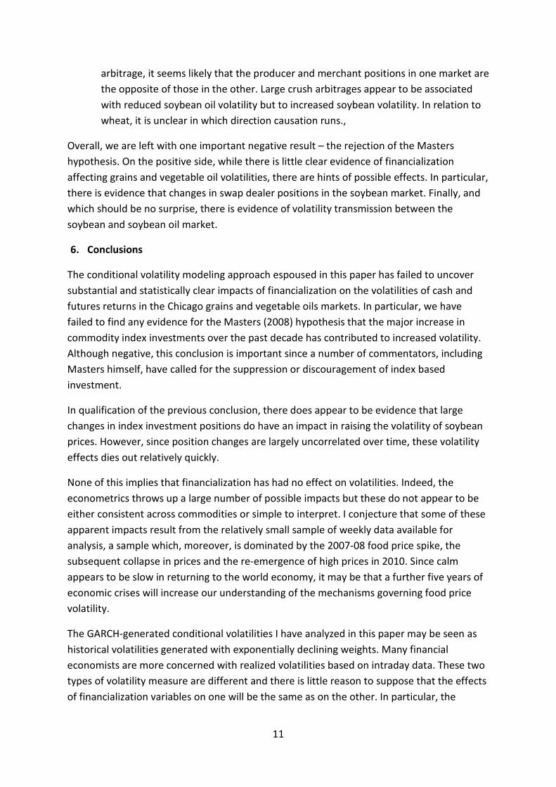
Because all futures transactions have counterparties, these five positions sum to zero identically. Figures 5-8 chart the net positions of these five groups and Table 2 reports descriptive statistics. The table also includes ADF statistics for both the position levels and changes and the first order autocorrelation coefficient of the changes.

In all four cases, producers and merchants were net short over the entire sample and swap dealers were net long by roughly the same order of magnitude. The small non-reporting group was always net short in the wheat, corn and soybean markets but this was not true of soybean oil. Money managers are generally but not invariably net long across all four markets whereas the pattern other reporting positions varies across the markets.

The Supplementals give information on index providers (CIT) positions. CIT positions largely fall within the swap provider category but a portion fall under money managers. Figure 9 charts these positions and Table 3 gives descriptive statistics. The largest, and also the most variable, CIT positions are in corn. The table also reports the correlations of changes in these positions with changes in the swap dealer and money manager positions which the CIT category overlaps. The swap dealer correlations range from 0.35 (soybeans) to 0.52

7

(soybean oil). The money manager correlations are much lower ranging from -0.07 (wheat) to 0.20 (soybeans).

The ADF statistics reported in Tables 2 and 3 show that the position change variables are all stationary. They are generally either positively autocorrelated with autocorrelation coefficients in the range 0.2 to 0.3, or, in the case of other reporting and non-reporting positions, have a small negative autocorrelation. The levels variables are more mixed – CIT positions appear non-stationary and the same is true of swap dealer positions, except in the case of wheat. The remaining levels variables are stationary.

4. Methodology

I adopt the GARCH(1,1) framework specified in equation (1) but add lagged position variables, here xt-1, one at a time, to the scedastic process:

( )( )

( )2

1 , 1 , 1 , , ,

0,1

t j jt jt

jt j j t j j j t j j t

jt

rj h

h rj h x j w c s o

N− − −

= κ + ε

= ω +α − κ +β + γ =

ε

(2)

This defines the GARCH-X model (Brenner et al, 1996). The test is the t-statistic on the coefficient γ of the lagged position variable.

The interpretation of this test is analogous to that of a Granger-causality test. If inclusion of a lagged position change variable in a GARCH equation enables us to better predict conditional volatilities, there must be a presumption of a causal link from the position change to the change in volatility. For this reason, I use the term GARCH-Granger test. As in the case of Granger-causality testing, an affirmative test result may arise if the position change is correlated with a third variable which is the genuine cause of the change in volatility. This qualification is important in the current context since position change variables are necessarily correlated by virtue of the fact that positions add to zero. As a consequence, any inference that the change in one position variable is the driver of volatility changes must be treated with caution.

A natural question is whether position changes are volatility-increasing or volatility-decreasing. This inference is also difficult. There are two reasons for this. The first follows from the previous discussion. Suppose we have only two trader categories, commercials and non-commercials. In this case, an increase in long non-commercial (speculative) positions must be exactly matched by an increase in short commercial (hedge) positions. If the estimated γ coefficient is positive for changes in speculative positions, apparently suggesting that an increase in speculative positions is volatility-increasing, it must be negative for hedge positions, suggesting that an increase in short hedge positions is also volatility-

8

decreasing. However, this casts no light on whether the causal impetus arises on the commercial or the non-commercial side, or even whether instead it is external.

The second problem is inherited from the Granger-causality framework. Granger-causality tests ask whether there is a causal impact from the candidate causal variable to the effect variable but are not informative about the sign of the causal relationship. Although it is natural in a testing framework, such as that in equation (2), which utilizes a single lag, to infer a positive impact if the estimated coefficient (here γ) on the lagged causal variable is positive, and a negative impact if the coefficient is negative, this may not be correct. One way in which this conclusion might be reversed is if the effect variable is in reality caused by contemporaneous changes in the causal variable which are, however, negatively autocorrelated. For this reason, inferences about the sign of any volatility impact need to take into account the serial correlation, if any, of the position changes.7

5. Results

Recall from Tables 2 and 3 that the producer and merchant, swap dealer, money manager and CIT position changes are all positively autocorrelated.

I first report test results where the X variable in the GARCH-X model is the lagged position change. I perform tests both on the volatility of cash returns and on returns on the first four futures contracts. Cash volatility is interesting because, if the convergence process is poorly functioning, it is possible that cash prices to differ substantially from futures prices. This appears to have been the case with wheat in 2008-09 – see Figure 1. Most studies look only at the front futures price. It is nevertheless worth looking at more distant futures since these will typically exhibit lower liquidity and this may result in the effects of position changes being more apparent.

Results are given in Table 4. They show only modest consistency across the four commodities considered.

• The clearest result is the negative relationship between lagged changes in other reporting positions and conditional volatility. This relationship is apparent in both the wheat and corn markets but not in either the soybean or soybean oil markets. It is true of cash corn as well as for the futures contracts, but the statistic is not statistically significant for cash wheat. The wheat and corn position changes exhibit very small and statistically insignificant autocorrelations (see Table 2) so we can be

7 A second possibility, which arises in an asset market context, is that the market shows “bounce” following large position changes. Suppose a position change causes a negative contemporaneous movement in a price or volatility but that this movement is wholly or partially reversed in the succeeding period. In this case, a Granger-type test will pick up the bounce which has the opposite sign from the original movement. Bounce seems more likely in relation to price levels than volatilities. I therefore ignore this possibility in the remainder of the paper.

9

reasonably secure in inferring that increases in the long positions (equally, decreases in the short positions) in other reporting positions are volatility-reducing.

• The corn results show a consistent negative relationship between lagged changes in CIT positions and conditional volatilities. This relationship is apparent for the three more distant futures contracts and also for the cash contract although the test statistic for the first future, which is typically the most liquid contract, is not significant. This relationship is not apparent for the other three commodities. On the contrary, there is some evidence in the opposite direction for third and fourth positions in wheat. Since CIT position changes are positively autocorrelated (see Table 2), we can be reasonably secure in inferring that increases in the long positions in CIT corn positions are volatility-reducing.

• For wheat only, there is some evidence that changes in lagged money market positions are positively associated with changes in conditional volatility. This evidence is clearest for the second and third futures positions which will typically be less liquid than the front contract.

• For soybean oil only, lagged changes in non-reporting positions are negatively associated with conditional volatilities. Since these positions are close to being serially independent, we can be reasonably secure in inferring that increases in the long positions (equally, decreases in the short positions) in non-reporting positions are volatility-reducing.

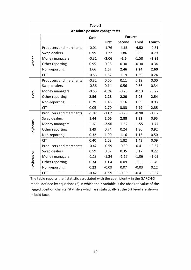
Volatility is a directionless measure or price variability. It may therefore be that it is the absolute size of position changes that matters and that the sign is irrelevant or misleading. In Table 5 I report the results of repeating the tests using these absolute measures.

• The negative relationship between lagged changes in other reporting positions for corn and conditional volatility reported in Table 4 becomes a positive relationship in Table 5. The less consistent relationship seen in Table 4 for wheat is not apparent in Table 5. The Table 5 results indicate that changes in the size of other reporting positions in corn have resulted in increased volatility. Estimates (not reported) which include both the lagged change and its absolute value give opposite and near equal coefficients so that the negative coefficient on the former cancels the positive coefficient on the latter for positive position changes. The results are therefore reconciled if it is that decreases, but not increases, in the long other reporting position (equally, rise in the short position) that are volatility increasing. It is difficult to make clear sense of this result.

• A similar situation, but with the signs reversed, for the effects of wheat money manager positions on conditional wheat volatilities. The implication is that results are therefore reconciled if it is increases, but not decreases, in the long money manager position are volatility increasing. Again, it is difficult to make clear sense of this result.

10

• The opposite situation arises for changes in corn index positions. Here, the estimated coefficients were significantly negative in Table 4 but are significantly positive in Table 5. Inclusion of both variables (results not reported) gives an insignificant estimate for the absolute position change indicating that the Table 4 results dominate.

• Differently from Table 4, the absolute values of lagged soybean swap dealer position changes is positively associated with conditional soybean volatilities. Large swap dealer position changes therefore appear to be volatility-increasing.

• The evidence in Table 4 of the effects of non-reporting position of soybean oil volatility is absent in Table 5. However, there is evidence, particularly from the more distant futures, that increases in the size of non-reporting positions in wheat may have been volatility-increasing.

Consideration of the evidence from Tables 4 and 5 jointly, the sole secure result is that changes in corn CIT positions have tended to be volatility increasing. Table 3 and Figure 9 both show the highest level of variability of corn CIT positions. This high variability may make it easier to discern the volatility impact of CIT position changes than in the other three commodities under consideration. The remaining relationships seen to be statistically significant in Tables 4 and 5 are difficult to rationalize and may result from sample correlations which will not necessarily be sustained in the future. Although 279 observations might in principle seem to constitute a long sample, Figures 1-4 show a relatively small number of large swings in conditional volatility.

In the final set of tests I use the lagged (absolute) level of positions as the X variable in the GARCH-X model.8

Results are reported in Table 7:

This allows me to examine whether a large overhang from one or another position reduces volatility by providing liquidity or raises volatility by “eating liquidity”. It therefore enables a direct test of the Masters (2008) hypothesis that CIT positions, as distinct from trades, are volatility-increasing. However, since the level variables are in general non-stationary (see Tables 2 and 3), these tests cannot sustain a Granger-type interpretation. In what follows, I therefore avoid offering any causal interpretation.

• Looking first at the Masters hypothesis, the coefficients on the lagged CIT position levels are nowhere significant. I conclude that there is no evidence for the claim that CIT positions are volatility increasing.

• There is evidence that a high level of (short) producer and merchant positions is volatility-increasing for wheat and soybeans, but volatility-decreasing for soybean oil. For the soybean and soybean oil markets, which are linked by the famous “crush”

8 Use of the absolute value of the level only makes a difference to the test outcomes for money manager and other reporting positions (plus non-reporting positions for soybean oil only), since the other position variables maintain the same sign throughout the sample – see Tables 2 and 3.

11

arbitrage, it seems likely that the producer and merchant positions in one market are the opposite of those in the other. Large crush arbitrages appear to be associated with reduced soybean oil volatility but to increased soybean volatility. In relation to wheat, it is unclear in which direction causation runs.,

Overall, we are left with one important negative result – the rejection of the Masters hypothesis. On the positive side, while there is little clear evidence of financialization affecting grains and vegetable oil volatilities, there are hints of possible effects. In particular, there is evidence that changes in swap dealer positions in the soybean market. Finally, and which should be no surprise, there is evidence of volatility transmission between the soybean and soybean oil market.

6. Conclusions

The conditional volatility modeling approach espoused in this paper has failed to uncover substantial and statistically clear impacts of financialization on the volatilities of cash and futures returns in the Chicago grains and vegetable oils markets. In particular, we have failed to find any evidence for the Masters (2008) hypothesis that the major increase in commodity index investments over the past decade has contributed to increased volatility. Although negative, this conclusion is important since a number of commentators, including Masters himself, have called for the suppression or discouragement of index based investment.

In qualification of the previous conclusion, there does appear to be evidence that large changes in index investment positions do have an impact in raising the volatility of soybean prices. However, since position changes are largely uncorrelated over time, these volatility effects dies out relatively quickly.

None of this implies that financialization has had no effect on volatilities. Indeed, the econometrics throws up a large number of possible impacts but these do not appear to be either consistent across commodities or simple to interpret. I conjecture that some of these apparent impacts result from the relatively small sample of weekly data available for analysis, a sample which, moreover, is dominated by the 2007-08 food price spike, the subsequent collapse in prices and the re-emergence of high prices in 2010. Since calm appears to be slow in returning to the world economy, it may be that a further five years of economic crises will increase our understanding of the mechanisms governing food price volatility.

The GARCH-generated conditional volatilities I have analyzed in this paper may be seen as historical volatilities generated with exponentially declining weights. Many financial economists are more concerned with realized volatilities based on intraday data. These two types of volatility measure are different and there is little reason to suppose that the effects of financialization variables on one will be the same as on the other. In particular, the

12

effects of financialization on market liquidity are more likely to be seen through examination of realized volatility whereas the conditional volatility measures considered in this paper, based on weekly data, will be more relevant for farmers, consumers and agricultural policy makers. The reconciliation of financialization impacts measured from data of the type we have used here and those from the analysis of intraday and trade (“tick”) data forms and important agenda item for ongoing research.

For this and other reasons, the results reported in this paper should be seen as a jumping off board for future research. I have noted that a number of the findings in the paper may not be sustained as the sample is lengthened. Other effects, such as that of the volatility impact of index-based trades on soybean volatility, may become more precisely estimated and the results may extend more generally. In any case, markets do not do the econometrician the service of standing still, and it is likely that, as they evolve, new issues and controversies will emerge. The academic and policy consensus therefore tends to reflect past realities. The role of empirically-based papers is to move that consensus towards the shifting frontier of market practice.

13

References Black, F. (1976), “The pricing of commodity contracts”, Journal of Financial Economics, 3,

167-179. Bollerslev, T. (1986), “Generalized autoregressive conditional heteroskedasticity”, Journal of

Econometrics, 31, 307-27. Brenner, R.J., R.H. Harjes and K.F. Kroner (1996), “Another look at models of the short-term

interest rate,” Journal of Financial and Quantitative Analysis, 31, 85-107. Caballero, R.J., E. Fahri and P-O. Gourinchas (2008a), “Financial crash, commodity prices and

global imbalances,” Brookings Papers on Economic Activity, Fall, 1-55. Caballero, R.J., E. Fahri and P-O. Gourinchas (2008b), “An equilibrium model of ‘global

imbalances’ and low interest rates,” American Economic Review, 92, 358-393. CFTC (2006), Commission Actions in Response to the “Comprehensive Review of the

Commitments of Traders Reporting Program (June 21, 2006), Washington DC, CFTC. De Long, J.B., A. Shleifer, L.H. Summers and R.J. Waldman (1990), “Positive feedback

investment strategies and destabilizing rational expectations”, Journal of Finance, 45, 379-95.

Diba, B., and Grossman, H. (1988) “The theory of rational bubbles in stock prices,” Economic Journal, 98, 746-754.

Fama, E.F. (1965), “The behavior of stock market prices”, Journal of Business, 38, 34-105. Friedman, M. (1953), Essays in Positive Economics, Chicago, University of Chicago Press,

157-203. Gilbert, C.L. (2010a), “How to understand high food prices”, Journal of Agricultural

Economics, 61, 398-425. Gilbert, C.L (2010b), “Speculative influence on commodity prices 2006-08”, Discussion Paper

197, UNCTAD, Geneva. Gilbert, C.L. (2010c), “Commodity speculation and commodity investment”, Commodity

Market Review, 2009-10, FAO, Rome. Gilbert, C.L. (2011), “International commodity agreements”, chapter 11 of A. Prakash ed.,

Safeguarding Food Security in Volatile Global Markets, Rome, FAO, 211-239. Gilbert, C.L., and S. Pfuderer (2012), “Index funds do impact futures prices”, paper

submitted to the Money, Macro and Finance Study Group workshop on commodity markets, May 2012.

Granger, C.W.J. (2007), “Causality in economics”, chapter 15 of P. Machamer and G. Wolters eds., Thinking about Causes, Pittsburgh, University of Pittsburgh Press.

Gorton, G., and K.G. Rouwenhorst (2006), “Facts and fantasies about commodity futures”, Financial Analysts Journal, 62, 47-68.

Irwin, S.H., P. Garcia, D.L. Good and E.L. Kunda (2009), “Poor convergence problems of CBOT corn, soybean and wheat futures contracts: causes and solutions”, Marketing and Outlook Research Report 2009-02, Department of Agricultural and Consumer Economics, University of Illinois at Urbana-Champaign.

14

Masters, M.W. (2008), Testimony before the U.S. Senate Committee of Homeland Security and Government Affairs, Washington, DC, 20 May 2008.

Mayer, J. (2011), “Financialized commodity markets: the role of information and policy issues”, Économie Appliquée, 44, 5-34.

Parkinson, M. (1980), “The extreme value method for measuring the variance of the rate of return”, Journal of Business, 53, 61-65.

Sanders, D. R. and S.H. Irwin (2010), “A speculative bubble in commodity futures prices? Cross-sectional evidence”, Agricultural Economics, 41, 25-32.

Sanders, D. R. and S.H. Irwin (2011), New Evidence on the impact of index funds in U.S. grain futures markets”, Canadian Journal of Agricultural Economics, 59, 519–532.

Stoll, H.R., and R.E. Whaley, (2010), “Commodity index investing and commodity futures prices”, Journal of Applied Finance, 20, 7-46.

Stoll, H.R., and R.E. Whaley, (2011), “Commodity index investing: speculation or diversification?”, Journal of Alternative Investments, 14, 50-60.

15

Table 1 Volatility descriptive statistics

Cash 1st future 2nd future 3rd future 4th future

Whe

at Average 49.4% 42.0% 41.3% 38.9% 35.3%

s.d. 11.2% 1.0% 3.2% 3.7% 4.3%

Correlation 0.529 1.000 0.848 0.740 0.818

Corn

Average 40.5% 39.3% 38.2% 36.4% 34.5%

s.d. 7.8% 4.1% 4.7% 5.2% 5.9%

Correlation 0.894 1.000 0.988 0.973 0.954

Soyb

eans

Average 30.1% 28.0% 27.8% 27.6% 27.4%

s.d. 9.8% 8.9% 8.8% 8.7% 8.6%

Correlation 0.988 1.000 0.997 0.997 0.996

Soyb

ean

oil Average 30.1% 27.9% 27.6% 27.5% 27.4%

s.d. 9.7% 9.0% 8.9% 8.8% 8.6%

Correlation 0.990 1.000 0.999 0.997 0.997

The table reports descriptive statistics associated with the conditional GARCH(1,1) volatilities graphed in Figures 1-4. In each case, the correlation is with the first future volatility. Sample: 13 June 2006 to 11 October 2011 (279 weekly observations)

16

Table 2 Position descriptive statistics

Producers and merchants

Swap dealers

Money managers

Other reporting

Non-reporting

Whe

at

Average -0.31 0.38 0.03 -0.04 -0.06 s.d. 0.05 0.03 0.06 0.02 0.02 Maximum -0.19 0.45 0.15 0.01 -0.01 Minimum -0.41 0.31 -0.12 -0.10 -0.09 ADF level -4.30 (1) -5.02 (1) -3.60 (1) -3.66 (0) -2.87 (1) ADF change -11.7 (1) -9.73 (2) -9.97 (3) -13.0 (1) -20.2 (1) AR(1) 0.26 0.20 0.26 -0.01 -0.20

Corn

Average -0.35 0.25 0.13 0.05 -0.08 s.d. 0.08 0.06 0.07 0.03 0.03 Maximum -0.14 0.35 0.26 0.11 -0.04 Minimum -0.52 0.12 -0.03 -0.04 -0.14 ADF level -2.95 (1) -1.41 (1) -3.25 (1) -2.24 (0) -2.11 (3) ADF change -12.0 (0) -12.2 (0) -12.1 (0) -16.9 (0) -8.43 (2) AR(1) 0.31 0.30 0.30 -0.02 -0.04

Soyb

eans

Average -0.37 0.26 0.14 0.04 -0.07 s.d. 0.11 0.04 0.08 0.04 0.02 Maximum -0.08 0.34 0.27 0.13 -0.01 Minimum -0.55 0.14 -0.12 -0.06 -0.13 ADF level -2.94 (2) -1.16 (3) -3.71 (1) -2.51 (1) -3.52 (1) ADF change -11.3 (1) -11.4 (2) -11.41 (1) -14.8 (0) -10.8 (2) AR(1) 0.27 0.20 0.23 0.11 0.07

Soyb

ean

oil

Average -0.39 0.24 0.10 0.01 0.03 s.d. 0.14 0.05 0.09 0.03 0.02 Maximum -0.04 0.37 0.27 0.09 0.07 Minimum -0.60 0.13 -0.13 -0.06 -0.03 ADF level -2.97 (1) -2.85 (1) -3.84 (1) -3.38 (0) -4.11 (1) ADF change -12.7 (0) -15.0 (0) -11.9 (0) -16.2 (0) -16.1 (0) AR(1) 0.25 0.10 0.32 0.02 0.02

The table reports descriptive statistics associated with the COT trader positions (millions of contracts) graphed in Figures 5-8. The order of the ADF test, chosen on the basis of the Akaike Information Criterion (AIC) is given in parentheses. The 5% critical value is -2.87. AR(1) is the first order autocorrelation coefficient of the position changes. Sample: 13 June 2006 to 11 October 2011 (279 weekly observations)

17

Table 3 CIT position descriptive statistics

Wheat Corn Soybeans Soybean oil Average 0.19 0.38 0.15 0.08 s.d. 0.02 0.07 0.03 0.02 Maximum 0.23 0.50 0.20 0.11 Minimum 0.13 0.22 0.09 0.04 SD correlation 0.49 0.57 0.35 0.52 MM correlation -0.07 0.10 0.20 0.08 ADF level -1.55 (1) -1.37 (1) -1.73 (1) -1.59 (1) ADF change -14.5 (0) -12.9 (0) -12.9 (0) -13.3 (0) AR(1) 0.13 0.24 0.23 0.21 The upper four rows of the table reports descriptive statistics associated with the CIT positions (millions of contracts) graphed in Figure 9. The middle two rows give the correlations of the CIT position changes with the changes in swap dealer (SD) and money manager (MM) positions over the same week. The order of the ADF test, chosen on the basis of the Akaike Information Criterion (AIC) is given in parentheses. The 5% critical value is -2.87. AR(1) is the first order autocorrelation coefficient of the position changes. Sample: 13 June 2006 to 11 October 2011 (279 weekly observations)

18

Table 4 Position change tests

Cash Futures

First Second Third Fourth

Whe

at

Producers and merchants -0.04 -0.62 -1.70 -2.12 -2.36 Swap dealers 2.66 1.79 1.97 2.28 2.64 Money managers -1.41 1.68 2.04 2.21 1.22 Other reporting -1.31 -2.42 -3.74 -3.95 -3.81 Non-reporting -1.10 -0.60 0.18 -0.03 0.55 CIT 1.63 -1.12 0.40 1.27 3.23

Corn

Producers and merchants 1.37 0.98 0.79 0.77 1.20 Swap dealers 0.33 0.50 0.35 -0.16 0.17 Money managers -0.01 1.07 -0.10 -0.14 -0.21 Other reporting -4.24 -3.75 -3.84 -3.93 -4.00 Non-reporting -0.83 -0.58 -0.43 -0.41 -0.31 CIT -2.69 -1.24 -2.32 -2.44 -2.27

Soyb

eans

Producers and merchants 0.28 0.38 0.15 1.77 0.78 Swap dealers -0.12 -0.57 -1.12 -0.74 -0.07 Money managers -0.14 -0.15 -0.20 -0.41 -0.65 Other reporting 0.07 0.42 1.20 0.87 -0.06 Non-reporting -0.45 -0.72 n.c. n.c. -0.64 CIT -1.56 -0.75 -0.80 -0.46 -1.89

Soyb

ean

oil

Producers and merchants 0.88 0.97 0.97 0.89 0.65 Swap dealers -0.83 -0.71 -0.71 -0.69 -0.71 Money managers -1.38 -1.70 -1.62 -1.73 -1.61 Other reporting 0.26 0.29 0.31 0.31 0.56 Non-reporting -2.43 -2.08 -2.07 -2.29 -2.04 CIT 0.88 0.97 0.97 0.89 0.65

The table reports the t statistic associated with the coefficient γ in the GARCH-X model defined by equations (2) in which the X variable is the lagged position change. Statistics which are statistically at the 5% level are shown in bold face. “n.c.” indicates no convergence.

19

Table 5 Absolute position change tests

Cash Futures

First Second Third Fourth

Whe

at

Producers and merchants -0.01 -1.76 -4.65 -4.52 -0.81 Swap dealers 0.99 -1.22 1.86 0.85 0.79 Money managers -0.31 -2.06 -2.5 -1.58 -2.95 Other reporting 0.95 0.38 0.30 -0.30 0.34 Non-reporting 1.66 1.67 2.46 2.24 2.60 CIT -0.53 1.82 1.19 1.59 0.24

Corn

Producers and merchants -0.32 0.00 0.11 0.19 0.00 Swap dealers -0.36 0.14 0.56 0.56 0.34 Money managers -0.53 -0.26 -0.23 -0.13 -0.27 Other reporting 2.56 2.28 2.20 2.08 2.54 Non-reporting 0.29 1.46 1.16 1.09 0.93 CIT 0.05 2.70 3.33 2.79 2.35

Soyb

eans

Producers and merchants -1.07 -1.02 -0.79 -0.98 -1.07 Swap dealers 1.44 2.06 2.88 2.32 0.95 Money managers -1.61 -2.96 -1.52 -1.55 -1.77 Other reporting 1.49 0.74 0.24 1.30 0.92 Non-reporting 0.32 1.00 1.16 1.13 0.50 CIT 0.40 1.08 1.82 1.43 0.09

Soyb

ean

oil

Producers and merchants -0.42 -0.59 -0.39 -0.41 -0.57 Swap dealers 0.59 0.07 0.35 0.17 0.22 Money managers -1.13 -1.24 -1.17 -1.06 -1.02 Other reporting 0.34 -0.04 0.09 0.05 -0.49 Non-reporting 0.23 -0.09 0.07 -0.03 0.12 CIT -0.42 -0.59 -0.39 -0.41 -0.57

The table reports the t statistic associated with the coefficient γ in the GARCH-X model defined by equations (2) in which the X variable is the absolute value of the lagged position change. Statistics which are statistically at the 5% level are shown in bold face.

20

Table 7 Absolute position level tests

Cash Futures

First Second Third Fourth

Whe

at

Producers and merchants 0.77 1.59 2.59 2.12 0.64 Swap dealers -0.46 -0.56 -0.52 0.01 -0.72 Money managers 0.59 0.15 0.29 1.01 0.61 Other reporting 1.72 0.12 0.22 0.66 0.89 Non-reporting -0.36 0.82 0.60 -0.21 0.83 CIT -1.58 -0.07 0.07 -0.54 -0.85

Corn

Producers and merchants 0.06 -0.10 -0.22 -0.07 -0.02 Swap dealers -0.81 -0.10 -0.19 -0.26 -0.28 Money managers 0.56 0.28 0.35 0.26 0.25 Other reporting -0.82 -2.12 -2.27 0.58 -2.23 Non-reporting 0.98 0.73 0.80 0.52 0.36 CIT -0.44 -1.24 -1.61 1.12 -0.20

Soyb

eans

Producers and merchants 2.21 2.57 9.70 5.83 2.55 Swap dealers -0.41 -0.55 -0.95 -0.96 -0.09 Money managers 1.64 2.62 3.23 2.83 2.34 Other reporting 0.26 0.60 0.91 0.87 0.56 Non-reporting 1.89 2.20 1.24 1.80 2.42 CIT 0.04 -0.01 0.62 0.24 0.45

Soyb

ean

oil

Producers and merchants -0.23 -2.66 -4.20 -6.71 -5.24 Swap dealers -0.05 -0.02 -0.30 -0.29 -0.29 Money managers -0.78 -0.79 -0.86 -0.85 -0.77 Other reporting -1.20 -1.21 -1.56 -1.62 -1.67 Non-reporting -0.35 -0.49 -0.31 -0.33 -0.26 CIT 0.15 0.20 0.47 0.51 0.45

The table reports the t statistic associated with the coefficient γ in the GARCH-X model defined by equations (2) in which the X variable is the absolute value of the lagged position level. Statistics which are statistically at the 5% level are shown in bold face.

21

Figure 1: Conditional wheat volatilities

Figure 2: Conditional corn volatilities

20%

30%

40%

50%

60%

70%

80%

90%

Cash1st future2nd future3rd future4th future

20%

30%

40%

50%

60%

70%

80%

90%

Cash1st future2nd future3rd future4th future

22

Figure 3: Conditional soybean volatilities

Figure 4: Conditional soybean oil volatilities

0%

10%

20%

30%

40%

50%

60%

70%

Cash1st future2nd future3rd future4th future

0%

10%

20%

30%

40%

50%

60%

70%

Cash1st future2nd future3rd future4th future

23

Figure 5: Wheat market positions

Figure 6: Corn market positions

-0.5

-0.4

-0.3

-0.2

-0.1

0.0

0.1

0.2

0.3

0.4

0.5

(mill

ion

cont

ract

s)Producers and merchants Swap dealers Money managers

Other reporting Non-reporting

-0.6

-0.5

-0.4

-0.3

-0.2

-0.1

0.0

0.1

0.2

0.3

0.4

(mill

ion

cont

ract

s)

Producers and merchants Swap dealers Money managers

Other reporting Non-reporting

24

Figure 7: Soybean market positions

Figure 8: Soybean oil market positions

-0.6

-0.5

-0.4

-0.3

-0.2

-0.1

0.0

0.1

0.2

0.3

0.4

(mill

ion

cont

ract

s)Producers and Merchants Swap dealers Money managers

Other reporting Non-reporting

-0.8

-0.6

-0.4

-0.2

0.0

0.2

0.4

0.6

(mill

ion

cont

ract

s)

Producers and merchants Swap dealers Money managers

Other reporting Non-reporting

25

Figure 9: Commodity Index Trader positions

0.0

0.1

0.2

0.3

0.4

0.5

0.6m

illio

n co

ntra

cts

Wheat_ChicagoCornSoybeansSoybean Oil