From Example 5.8-1,

Finally,

or, for 0.5 m of bed, AP = 0.42 mm Hg.

5.8-4 Vapor Capacity

Generalized correlations for flood point prediction have been based on the early work of Sherwood et al.19

Modifications of this work have been made from time to time, with that of Eckert,20 mentioned earlier inconnection with pressure drop estimation, being representative of those now in use. The flood line isdesignated as the top curve of Fig. 5.8-12. Thus, as for pressure drop, the Eckert chart enables a quickestimate of the maximum allowable vapor flow through the packed bed in question.

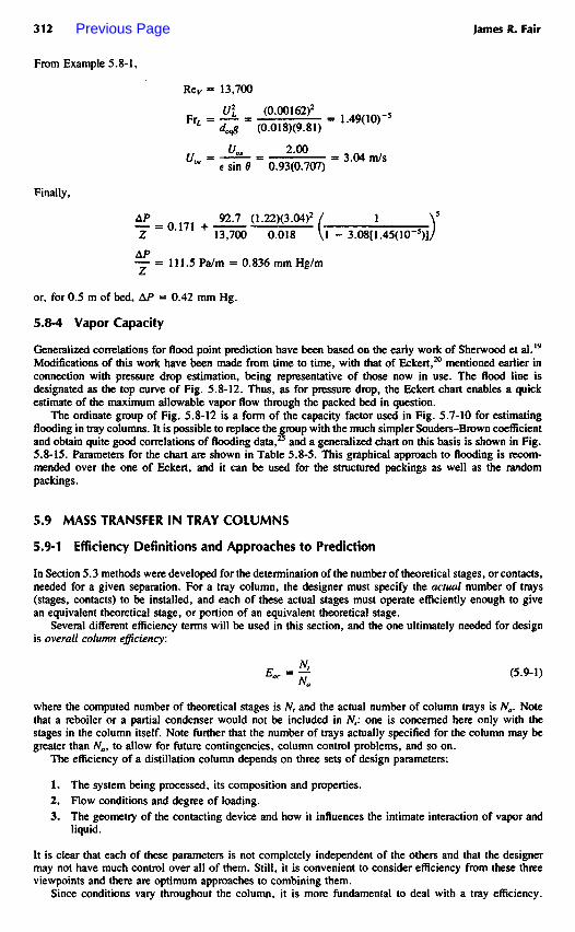
The ordinate group of Fig. 5.8-12 is a form of the capacity factor used in Fig. 5.7-10 for estimatingflooding in tray columns. It is possible to replace the group with the much simpler Souders-Brown coefficientand obtain quite good correlations of flooding data,25 and a generalized chart on this basis is shown in Fig.5.8-15. Parameters for the chart are shown in Table 5.8-5. This graphical approach to flooding is recom-mended over the one of Eckert, and it can be used for the structured packings as well as the randompackings.

5.9 MASS TRANSFER IN TRAY COLUMNS

5.9-1 Efficiency Definitions and Approaches to Prediction

In Section 5.3 methods were developed for the determination of the number of theoretical stages, or contacts,needed for a given separation. For a tray column, the designer must specify the actual number of trays(stages, contacts) to be installed, and each of these actual stages must operate efficiently enough to givean equivalent theoretical stage, or portion of an equivalent theoretical stage.

Several different efficiency terms will be used in this section, and the one ultimately needed for designis overall column efficiency:

(5.9-1)

where the computed number of theoretical stages is N, and the actual number of column trays is A .̂ Notethat a reboiler or a partial condenser would not be included in Nt: one is concerned here only with thestages in the column itself. Note further that the number of trays actually specified for the column may begreater than Nay to allow for future contingencies, column control problems, and so on.

The efficiency of a distillation column depends on three sets of design parameters:

1. The system being processed, its composition and properties.2. Flow conditions and degree of loading.3. The geometry of the contacting device and how it influences the intimate interaction of vapor and

liquid.

It is clear that each of these parameters is not completely independent of the others and that the designermay not have much control over all of them. Still, it is convenient to consider efficiency from these threeviewpoints and there are optimum approaches to combining them.

Since conditions vary throughout the column, it is more fundamental to deal with a tray efficiency.

Previous Page

Flow parameter, LIG (QVIQL)0'5

FIGURE 5.8-15 Design chart for packed column flooding. See Table 5.8-5 for factors of other packings.

2 in. Metal Pall rings1 1/2 in. Metal Pall rings1 in. Metal Pall rings

Ceramic Raschig rings

TABLE 5.8-5 Relative Flooding Capacities for Packed Columns Using 50 mm Pall Rings as theBasis

Pall Rings—Metal Intalox Saddles—Ceramic Koch Sulzer BX50 mm 1.00* 50 0.89 BX 1.0038 0.91 38 0.7525 0.70 25 0.60 Koch Flexipac12 0.65 12 0.40 N o j Q 6 9

Raschig Rings—Metal BeH Saddles—Ceramic N ° * 3 ^s

50 0.79 50 0.8438 0.71 38 0.70 Tellerettes25 0.66 25 0.54 , 0

12 0.55 12 0.37

, - «• -̂ • i r- j j i », i Nor-Pak PlasticRaschig Rings—Ceramic Intalox Saddles—Metal50 0.78 No. 25 0.88 JJo" 35 12038 0.65 No. 40 0.98 **25 0.50 No. 50 1.1012 0.37 No. 70 1.24

•Value is ratio of CSB for packing type and size to the CSB for 50 mm Pall rings for the same value offlow parameter.

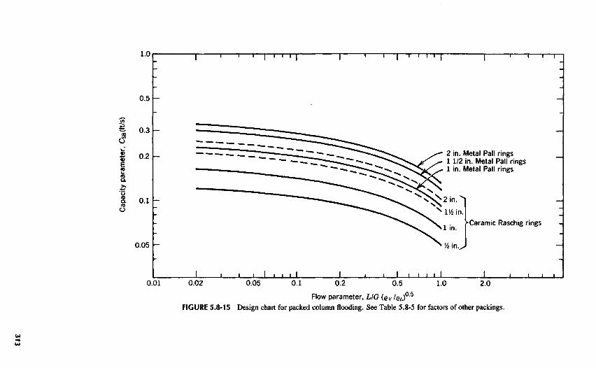
Figure 5.9-1 shows the vapor and liquid streams entering and leaving the nth tray in the column, and theefficiency of the vapor-liquid contact may be related to the approach to phase equilibrium between the twoexit streams:

(5.9-2)

where y* = KVLxn (Ky1 being the vapor-liquid equilibrium ratio discussed in Section 5.2) and the com-positions refer to one of the components in the mixture (often to the lighter component of a binary pair orto the "light key" of the mixture. The graphical equivalent of Eq. (5.9-2) is shown in Fig. 5.9-1, whereactual trays have been stepped off on a McCabe-Thiele-type diagram.

Equation (5.9-2) defines the Murphree vapor efficiency \ an equivalent expression could be given interms of liquid concentrations, but the vapor concentration basis is the one most used, and it is equivalentto its counterpart dealing with the liquid. It should be noted that the value of y* is based on the exitconcentration of the liquid and is silent on the idea that liquid concentration can vary from point to pointof the tray; when liquid concentration gradients are severe, as in the case of very long liquid flow paths,it is possible for the Murphree efficiency to have a value greater than 1.0.

A more fundamental efficiency expression deals with some point on the tray:

(5.9-3)

This is the local efficiency ox point efficiency, and because a liquid concentration gradient is not involved,it cannot have a value greater than 1.0. Thus, it is a more fundamental concept, but it suffers in applicationsince concentration profiles of operating trays are difficult to predict. As in the case of the Murphree trayefficiency, it is possible to use a liquid-phase point efficiency.

There are four general methods for predicting the efficiency of a commercial distillation column:

1. Comparison with a very similar installation for which performance data are available.2. Use of an empirical or statistical efficiency model.3. Direct scaleup from carefully designed laboratory or pilot plant experiments.4. Use of a theoretical or semitheoretical mass transfer model.

In practice, more than one of these methods will likely be used. For example, available data from a similarinstallation may be used for orientation and a theoretical model may then be used to extrapolate to the newconditions.

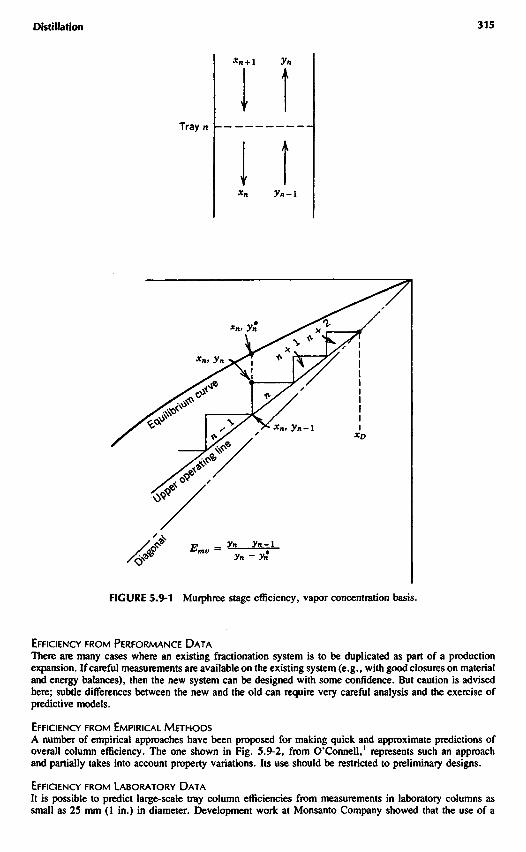
FIGURE 5.9-1 Murphree stage efficiency, vapor concentration basis.

EFFICIENCY FROM PERFORMANCE DATAThere are many cases where an existing fractionation system is to be duplicated as part of a productionexpansion. If careful measurements are available on the existing system (e.g., with good closures on materialand energy balances), then the new system can be designed with some confidence. But caution is advisedhere; subtle differences between the new and the old can require very careful analysis and the exercise ofpredictive models.

EFFICIENCY FROM EMPIRICAL METHODSA number of empirical approaches have been proposed for making quick and approximate predictions ofoverall column efficiency. The one shown in Fig. 5.9-2, from O'Connell,1 represents such an approachand partially takes into account property variations. Its use should be restricted to preliminary designs.

EFFICIENCY FROM LABORATORY DATAIt is possible to predict large-scale tray column efficiencies from measurements in laboratory columns assmall as 25 mm (1 in.) in diameter. Development work at Monsanto Company showed that the use of a

Tray

Relative volatility of key component X viscosity offeed (at average column conditions)

FIGURE 5.9-2 O'Connell method for the estimation of overall column efficiency (Ref. 1).

special laboratory sieve tray column, the Oldershaw column, produces separations very close to those thatcan be accomplished in the large equipment. A description of the underlying research is given by Fair etal.2 A view of a glass Oldershaw tray is shown in Fig. 5.9-3. Typical comparisons between Oldershawand commercial-scale efficiencies are shown in Fig. 5.9-4.

The Oldershaw testing provides values of the point efficiency. It is still necessary to correct thisefficiency to the Murphree and overall efficiencies, and approaches for this will be given later. For themoment it is important to consider the potential importance of the Oldershaw scaleup method: a specificdefinition of the system may not be necessary; the matter of vapor-liquid equilibria can be bypassed (ineffect, the Oldershaw column serves as a multiple-stage equilibrium still) and efficiency modeling can beminimized or even eliminated.

The procedure for using the Oldershaw scaleup approach is given in Ref. 2 and may be summarizedas follows:

1. Arbitrarily select a number of Oldershaw stages and set up the column in the laboratory. Oldershawcolumns and their auxiliaries are available from laboratory supply houses and are available in anumber of actual stages.

2. For the system to be studied, run the column and establish the upper operating limit (flood con-dition). Take data at a selected approach to flood, using total reflux or finite reflux. At steadyconditions, take overhead and bottom samples.

3. If the separation is satisfactory, the commercial column will require no more than the number ofstages used in the laboratory. Depending on the degree of liquid mixing expected, the large column

FIGURE 5.9-3 Glass Oldershaw tray, 50 mm diameter.

Plat

e ef

ficie

ncy,

%: Commercial hydrocarbonfractionation columnCommercial chlorinated hydrocarbonfractionation columnCommercial alcoholfractionationLaboratory fractionation ofethyl alcoholMiscellaneous

PERCENT FLOODFIGURE 5.9-4 Comparison of Oldershaw column (25 mm diameter) efficiency with that of a test columnat Fractionation Research, Inc. (FRI) of 1.2 m diameter (Ref. 2).

may require fewer stages. Note that comparisons must be made at the same approach to the floodpoint.

Unfortunately, a method such as this is not available for packed columns; more on this will be given inSection 5.10.

EFFICIENCY FROM MASS TRANSFER MODELS

Prediction of efficiency based on mass transfer theory and character of the two-phase contacting zone(Section 5.7-2) is a goal with parallels in other types of unit operations equipment. The development ofsuitable models for efficiency has been underway for a number of years, since the pioneering paper ofGeddes in 1946.3 From a practical point of view the first model suitable for design emerged from theAIChE Distillation Efficiency in 1958.4 As mentioned earlier, mass transfer models are useful not only fornew designs but for studying effects of changed operating conditions in existing designs.

5.9-2 Phase Transfer Rates

GENERAL EXPRESSIONS

Mass transfer on a distillation tray proceeds according to the general flux relationship:

(5.9-4)

where = flux of species A across a unit area of interface= mole fraction of A in bulk vapor= mole fraction of A in vapor at the interface= mole fraction of A in vapor that would be in equilibrium with mole fraction of A in bulk

liquid, xA

= mole fraction of A in liquid at the interface= mole fraction of A in liquid that would be in equilibrium with mole fraction of A in bulk

vapor, yA

Equation (5.9-4) may be written in a similar fashion for net transfer from liquid to vapor, and indeed indistillation there is usually a nearly equal number of total moles transferred in each direction. The masstransfer coefficients in Eq. (5.9-4) may be combined as follows:

(5.9-5)

and

EFFI

CIEN

CY,

Cyclohexane/n-Heptane

(5.9-6)

In these equations, m is the slope of the equilibrium line. For a binary system, and from Section 5.2, thisslope is

(5.9-7)

where aAB is the relative volatility and A is the lighter of the two components in the mixture. It can beshown that for a multicomponent system the pseudobinary value of m is equal to the equilibrium ratio KVL

for the lighter of the pseudocomponents.The mass transfer coefficients in Eq. (5.9-4) may be evaluated by various means. According to the film

model, and for the example of vapor-phase transfer,

(5.9-8)

where AZ is the thickness of the laminar-type film adjacent to the interface and Dv is the vapor-phasediffusion coefficient. For the penetration model,

(5.9-9)

where 9 is the time of exposure at the interface for an element of fluid that has the propensity to transfermass across the interface. Both film and penetration (or, alternatively, surface renewal) models are usedand differ primarily in the exponent on the diffusion coefficient. The weight of experimental evidencesupports the one-half power dependence, but neither the renewal time nor the film thickness is a parametereasily determined. Thus, models deal primarily with the mass transfer coefficients.

Even though tray columns are normally crossflow devices (as opposed to counterflow devices such aspacked columns), certain aspects of counterflow theory are used with trays. This involves the use of transferunits as measures of the difficulty of the separation. For a simple binary system, and for distillation, thenumber of transfer units may be obtained from

(5.9-10)

(5.9-11)

(5.9-12)

with heights of transfer units obtained from

(5.9-13)

(5.9-14)

(5.9-15)

Considering vapor-phase transfer as an example, and recognizing that Z = NyHy, the number of transferunits may be expressed as

(5.9-16)

In the context of a vapor passing up through the froth on a tray, this expression may be modified to

(5.9-17)

Note here that Eq. (5.7-6) has been used. Thus, the height of a vapor-phase transfer unit is Hv = Ualkva,*.In a similar fashion, and with the aid of Eq. (5.7-7), the number of liquid-phase transfer units may beobtained:

(5.9-18)

On the assumption that the transfer resistances of the phases are additive,

(5.9-19)

where X is the ratio of slopes of the equilibrium and operating lines; that is,

(5.9-20)

Thus, the slope of the operating line is obtained from equilibrium stage calculations and the slope of theequilibrium line is obtained as discussed above.

When Noy is evaluated at a point on the tray, the basic expression for point efficiency is obtained:

(5.9-21)

LIQUID-PHASE MASS TRANSFEREquation (5.9-18) is used to obtain values of NL. The residence time for liquid in the froth or spray isobtained from Eq. (5.7-9). For sieve trays, the experimental correlation of Foss and Gerster,5 included inRef. 4, is recommended:

(5.9-22)

For bubble-cap trays,

(5.9-23)

In these equations, D^ is the liquid-phase molecular diffusion coefficient, in m2/s, and the volumetriccoefficient kLat has units of reciprocal seconds.

VAPOR-PHASE MASS TRANSFERIn distillation the vapor-phase resistance to mass transfer often controls and thus the estimation of vapor-phase transfer units tends to be a critical issue. Equation (5.9-17) is used to evaluate the number of transferunits, and residence time is obtained from Eq. (5.7-6) or (5.7-8). The volumetric mass transfer coefficientis obtained from the expression of Chan and Fair:6

(5.9-24)

In this expression, the volumetric mass transfer coefficient is in reciprocal seconds, the molecular diffusioncoefficient in m2/s, and the liquid holdup h'L in meters. The term F refers to fractional approach toflooding.

For bubble-cap trays, the expression developed by the AIChE4 should be used to obtain the number oftransfer units directly:

(5.9-25)

w h e r e w e i r height, mmF factor through active portion of tray, m/s(kg/m3)l/2

liquid flow rate, m3 /sm, of width of flow path on the trayvapor-phase Schmidt number, dimensionless

5.9-3 Local Efficiency

Once the vapor- and liquid-phase transfer units have been determined, they are combined to obtain thenumber of overall transfer units (vapor concentration basis) by Eq. (5.9-19). Finally, the local, or point,efficiency is computed:

(5.9-21)

The next step in the process is to correct this point efficiency for vapor and liquid mixing effects.

5.9-4 Liquid and Vapor Mixing

The concentration gradients in the liquid and vapor on the tray are analyzed to determine whether the pointefficiency needs correction to give the Murphree efficiency. If the phases are well mixed, and no concen-tration gradients exist,

(complete mixing) (5.9-26)

If the liquid moves across the tray in plug flow, and the vapor rising through it becomes completely mixedbefore entering the tray above,

(5.9-27)

Thus, it is necessary to consider tray mixing effects to arrive at a value of Emv for design. Entrapmenteffects also must be considered, as discussed in Section 5.7-4. A chart showing the overall developmentof a design sequence is shown in Fig. 5.9-5.

For trays with relatively narrow spacing, the vapor may not be able to mix completely before leavingthe tray. For the case of plug flow of liquid and nonmixing of vapor, and with liquid alternating in flowdirection on successive trays, representative effects of vapor mixing are shown in Table 5.9-1. A morecomplete view of mixing effects may be seen in Fig. 5.9-6.8

The partial liquid mixing case is of considerable interest in design. Various models for representingpartial mixing have been proposed: for most instances the eddy diffusion model appears appropriate. Thismodel uses a dimensionless Peclet number:

Physical Flow DeviceProperties Conditions Geometry

L ^ 1 _ J

ZoneCharacteristics (Regimes)

ILocal

Efficiency (EOv)

1

Liquid VaporMixing Mixing

1 • > • 'Dry Murphree

Efficiency

IWet Murphree

EfficiencyFIGURE 5.9-5 Sequence of steps for evaluating the overall tray efficiency or for deducing the pointefficiency.

TABLE 5.9-1 Effect of Vapor Mixing on Plug Flow Efficiency

Plug

Eov Vapor Mixed Vapor Unmixed

0.60 0.82 0.810.70 1.02 0.980.80 1.22 1.16

(5.9-28)

where w' is the length of travel across the tray. A high value of the Peclet number indicates a close approachto plug flow. As the Peclet number approaches zero, complete mixing is approached. The relationshipbetween Emv, Eov, and Pe is shown in Fig. 5.9-7.

A simpler approach uses the mixing pool model of Gautreaux and CTConnell.9 These workers visualizeda crossflow tray as being comprised of a number of well-mixed stages, or mixing pools, in series. Theirgeneral expression for mixing is

(5.9-29)

where J, the number of pools, was estimated by Gautreaux and O'Connell to be some function of lengthof liquid path. It is more convenient to estimate 5 as a function of Peclet number:

(5.9-30)

which is simpler than using Fig. 5.9-7.It still remains that an estimate of the eddy diffusion coefficient must be made to evaluate the Peclet

number. For sieve trays the work of Barker and Self10 is appropriate:

(5.9-31)

For bubble-cap trays, the AIChE work4 provides the following:

(5.9-32)

Equations (5.9-31) and (5.9-32) are based on unidirectional flow, the expected situation for the rect-angular simulators that were used in the experiments. For large-diameter trays, there can be serious retro-grade flow effects, with resulting loss of efficiency due to stagnant zones. The work of Porter et al .n andBell12 elucidates the retrograde flow phenomenon, but the efficiency loss appears to be important only forcolumn diameters of 5 m or larger, especially for relatively short segmental weirs.

5.9-5 Overall Column Efficiency

As indicated in Fig. 5.9-6, overall column efficiency is obtained from the Murphree efficiency Emv (or fromthe Murphree efficiency corrected for entrainment, Ea). The conversion is by the relationships

(5.9-33)

5.9-5 Multicomponent Systems

The foregoing material is based on studies of binary systems. For such systems the efficiency for eachcomponent is the same. When more than two components are present, it is possible for each componentto have a different efficiency. Examples of efficiency distribution in multicomponent systems are given in

(C)

FIGURE 5.9-6 Relationship between point efficiency and Muiphnee efficiency for three cases of liquid-vapor flow combinations. Liquid in plug flow in all cases (Ref. 8). (a) Relationship of point efficiency toMurphree plate efficiency. Case 1: Vapor mixed under each plate, (b) Relationship of point efficiency toMurphree plate efficiency. Case 2: Vapor not mixed; flow direction of liquid reversed on successive plates,(c) Relationship of point efficiency to Murphree plate efficiency. Case 3: Vapor not mixed; liquid flow insame direction on successive plates.

Point efficiency, Eou

(a) (b)

E0O

Em

v

Ove

rall

Mu

rph

ree

vapo

r ef

ficie

ncy

of a

sin

gle

plat

e,

(b)

FIGURE 5.9-7 Relationship between point and Murphree efficiencies for partial mixing of liquid andcomplete mixing of vapor (Ref. 4).

the experimental results of Young and Weber," Krishna et al.,14 and Chan and Fair.15 For ideal systemsthe spread in efficiency is normally small.

The basic theory for multicomponent system efficiency determination has been given by Toor andBurchard16 and by Krishna et al.l4 In a series of experiments, confirmed by theory, Chan and Fair determinedthat a good approximation of multicomponent efficiency may be obtained by considering the dominant pairof components at the location in the column under consideration. This permits use of a pseudobinaryapproach, undoubtedly realistic for most commercial designs.

5.10 MASS TRANSFER IN PACKED COLUMNS

5.10-1 Efficiency Definitions and Approaches to Prediction

For packed columns, which are classified as counterflow columns (most trays are crossflow devices), masstransfer is related to transfer rates in counterflow vapor-liquid contacting. The most-used criterion ofefficiency is the height equivalent to a theoretical plate (HETP) that was first introduced by Peters:1

H E T P . Height of packed zoneNumber of theoretical stages achieved m zone

In using this expression to determine the required height of packing, one would calculate the number ofideal stages (Section 5.3) and obtain a value of HETP (likely from a packing vendor); the height of packingwould then follow directly.

Alternately, the height of packing may be obtained by a more fundamental approach, the use of transferunits;

(5.10-2)

where Hv, Hu Hoy, and HOL are known as "heights of a transfer unit" (HTU) based on vapor-phase,

liquid-phase, and combined-phase concentration driving forces, respectively. In the present work, a vapor-phase concentration basis will be adopted, and thus the term HOL will not be used. The equivalent "numbersof transfer units,*' /VV, NL, and NOVy will also be used.

As is the case for a tray column, the efficiency depends on the system properties, the flow conditions,and the geometry of the device. Because of the many possible variations in the geometry of the packedbed, the last-named parameter assumes great importance in the estimation of packed column efficiency.

Methods for predicting efficiency also parallel those for tray columns: comparison against a similarinstallation, use of empirical methods, direct scaleup from laboratory or pilot plant, and use of theoreticallyderived models. Approaches by vendors of packing usually center on comparisons with similar installations(the so-called "vendor experience") and empirical approximations. Direct scaleup from small columnstudies is difficult with packed columns because of the unknown effects of geometrical factors and thevariations of liquid distribution that are required for practical reasons. Theoretical or semitheoretical modelsare difficult to validate because of the flow effects on interfacial area. It may be concluded that there is noveiy good way to predict packed column efficiency, at least for the random type packings.

The approach used in the present work is that of semitheoretical models for mass transfer prediction.The reader should remember, however, that the packing vendors should be consulted as early as possible.These people have a great deal of experience with their own packings and, in addition, have done a greatdeal of their own test work. The models can then be used in connection with the vendor information toarrive at a final design.

5.10-2 Vendor Information

Vendors can provide values of HETP on the basis of their experience. They also conduct controlled testson packings, using as a basis the absorption of carbon dioxide from air into a dilute solution of sodiumhydroxide. The results of such tests normally are given in terms of an overall volumetric mass transfercoefficient, Kova. A discussion of the test method has been provided by Eckert et al.2 Because a reactionoccurs in the liquid phase, and because the rate of the reaction is a function of the degree of conversionof the hydroxide to the carbonate, it is difficult to construe the test results in terms of distillation needs.Also, the process involves significant mass transfer resistance in both the gas and liquid phases. As a result,such test values should be used with caution and, in general, considered only as a guide to the relativeefficiencies of different packings.

Some vendors also have conducted their own tests under distillation conditions and can make such testdata available. This is particularly the case for the vendors of structured packings. Standard distillation testmixtures are used, with operation usually under total reflux conditions. The use of these data, in connectionwith a mass transfer model, enables the most reliable approach to the estimation of the efficiency that apacked bed will produce.

5.10-3 Mass Transfer Models

For distillation, the height of a transfer unit is defined as

(5.10-3)

(5.10-4)

(5.10-5)

A combination of these units leads to

(5.10-6)

This approach enables one to consider separately the vapor- and liquid-phase mass transfer characteristicsof the system and the packing.

RANDOM PACKINGS

Several methods have been proposed for predicting values of Hv and HL as functions of system, flowconditions, and packing type. These include the methods of Cornell et al.,3 Onda et al.,4 Bravo and Fair,5

and Bolles and Fair.67 The last-named has had the broadest validation and will be discussed here.The Bolles-Fair method may be summarized by the following equations:

(5.10-7)

(5.10-8)

(5.10-9)

(5.10-10)

(5.10-11)

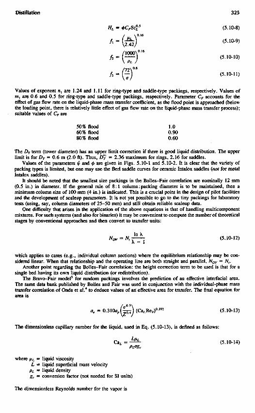
Values of exponent /i, are 1.24 and 1.11 for ring-type and saddle-type packings, respectively. Values ofmx are 0.6 and 0.5 for ring-type and saddle-type packings, respectively. Parameter CF accounts for theeffect of gas flow rate on the liquid-phase mass transfer coefficient, as the flood point is approached (belowthe loading point, there is relatively little effect of gas flow rate on the liquid-phase mass transfer process);suitable values of CF are

50% flood 1.060% flood 0.9080% flood 0.60

The DT term (tower diameter) has an upper limit correction if there is good liquid distribution. The upperlimit is for DT = 0.6 m (2.0 ft). Thus, D? = 2.36 maximum for rings, 2.16 for saddles.

Values of the parameters ^ and <f> are given in Figs. 5.10-1 and 5.10-2. It is clear that the variety ofpacking types is limited, but one may use the Berl saddle curves for ceramic Intalox saddles (not for metalIntalox saddles).

It should be noted that the smallest size packings in the Bolles-Fair correlation are nominally 12 mm(0.5 in.) in diameter. If the general rule of 8:1 column: packing diameter is to be maintained, then aminimum column size of 100 mm (4 in.) is indicated. This is a crucial point in the design of pilot facilitiesand the development of scaleup parameters. It is not yet possible to go to the tiny packings for laboratorytests (using, say, column diameters of 25-50 mm) and still obtain reliable scaleup data.

One difficulty that arises in the application of the above equations is that of handling multicomponentmixtures. For such systems (and also for binaries) it may be convenient to compute the number of theoreticalstages by conventional approaches and then convert to transfer units:

(5.10-12)

which applies to cases (e.g., individual column sections) where the equilibrium relationship may be con-sidered linear. When that relationship and the operating line are both straight and parallel, Nov = Nt.

Another point regarding the Bolles-Fair correlation: the height correction term to be used is that for asingle bed having its own liquid distribution (or redistribution).

The Bravo-Fair model5 for random packings involves the prediction of an effective interfacial area.The same data bank published by Bolles and Fair was used in conjunction with the individual-phase masstransfer correlation of Onda et al.4 to deduce values of an effective area for transfer. The final equation forarea is

(5.10-13)

The dimensionless capillary number for the liquid, used in Eq. (5.10-13), is defined as follows:

(5.10-14)

where fiL = liquid viscosityL - liquid superficial mass velocity

pL = liquid densitygc = conversion factor (not needed for SI units)

The dimensionless Reynolds number for the vapor is

PERCENT FLOOD

FIGURE 5.10-1 Packing parameters for estimating vapor-phase mass transfer, random packings (Ref. 7).

(5.10-15)

This model was found to give a slightly better fit of the distillation data than did the Bolles-Fair model.It is somewhat more cumbersome to use, however, because of the need to evaluate individual-phase transfercoefficients.

STRUCTURED PACKINGSThe channels formed by the structured packing elements are presumed to pass liquid and vapor in coun-terflow contacting. Since the geometry is well defined and the packing surface area is known precisely, ithas been found possible to model the mass transfer process along lines of wetted wall theory. The followingmaterial is based on recent work by Bravo et al.8 at the University of Texas and has been developedspecifically for structured packings of the gauze type, the principal dimensions of which are listed in Table5.10-1.

Using Fig. 5.8-14 as a guide, the equivalent diameter of a channel is defined as

(5.10-16)

where B = base of the triangle (channel cross section)h = height of the triangle ("crimp height")5 = corrugation spacing (channel side)

Metal PALL® Rings

Ceramic Berl Saddles

PACK

ING

PARA

MET

ER,

Metal Raschig Rings

Ceramic Raschig Ringsi i i

MASS VELOCITY, GL. lbm/(h)(ft2)FIGURE 5.10-2 Packing parameters for estimating liquid-phase mass transfer, random packings (Ref. 7).{Note: The value of <£ from the chart is in feet. (lbm/h-ft2) x 0.00136 = kg/s-m2.)

TABLE 5.10-1 Geometric Information, Sulzer BX Packing

Crimp height, h (mm) 6.4Channel base, B (mm) 12.7Channel side, S (mm) 8.9Hydraulic radius, rh (mm) 1.8Equivalent diameter, d^ (mm) 7.2Packing surface, ap (m2/m3) 492Void fraction, € 0.90Channel flow angle from horizontal (degrees) 60

Ceramic Raschig Rings

Metal Raschig Rings

PACK

ING

PARA

MET

ER,

Ceramic Berl Saddles

Metal PALL® Rings

The effective velocity of vapor through the channel is

(5.10-17)

The effective liquid velocity is based on the falling film relationship for laminar flow:

(5.10-18)

where T = LIPAn kg/s • m perimeterA, = tower cross-sectional area, m2

P = available perimeter, m/m2, tower cross section= l/2[(45 + 2B)IBh + ASIU]

For the vapor-phase mass transfer coefficient, the early work of Johnstone and Pigford9 is used in a slightlymodified form:

(5.10-19)

where Sh v = Sherwood number for the vapor = kydeqIDv

Key - Reynolds number for the vapor, defined for the present geometry as (dc<ipy/fXy)(Uve + Uu)Scv — Schmidt number for the vapor = \kylpvD

v

For the liquid phase, the penetration theory is used, with one exposure being the residence time for liquidflow between corrugation changes:

(5.10-20)

Finally, an analysis of the experimental data on the gauze-type structured packing showed that the totalsurface was fully wetted. This was attributed in part to the capillary action that takes place with the finelywoven wire gauze.

Thus, heights of transfer units can be calculated for the structured packing case, using information fromthe above relationships. The method was checked against 132 data points and found to have an averagedeviation of 14.6%.

Methods for handling the sheet metal structured packings have not yet been published. However, itseems clear that such packings do not have the benefit of capillary action and thus may not be completelywetted. General experience shows that the same approach may be used but that the transfer area must bediscounted to about 60% of the specific surface area of the packing. Under high loading conditions, theamount of discount is likely to be much less.

5.11 DISTILLATION COLUMN CONTROL

The control of distillation systems is a subject that has been treated extensively in the literature. At leastfour books on distillation control have been published in recent years.1"4 It is appropriate that in the presentwork only a few general guidelines on control be presented.

The column variables of concern, in a simple one-feed two-product column with pressure controlledseparately, may be categorized as follows:

1. Controlled Variables(a) Throughput(b) Distillate composition(c) Bottoms composition(d) Bottoms sump level(e) Reflux accumulator level

2. Manipulated Variables(a) Feed flow(b) Distillate flow

(c) Reflux flow

(d) Heat medium flow

(e) Bottoms flow

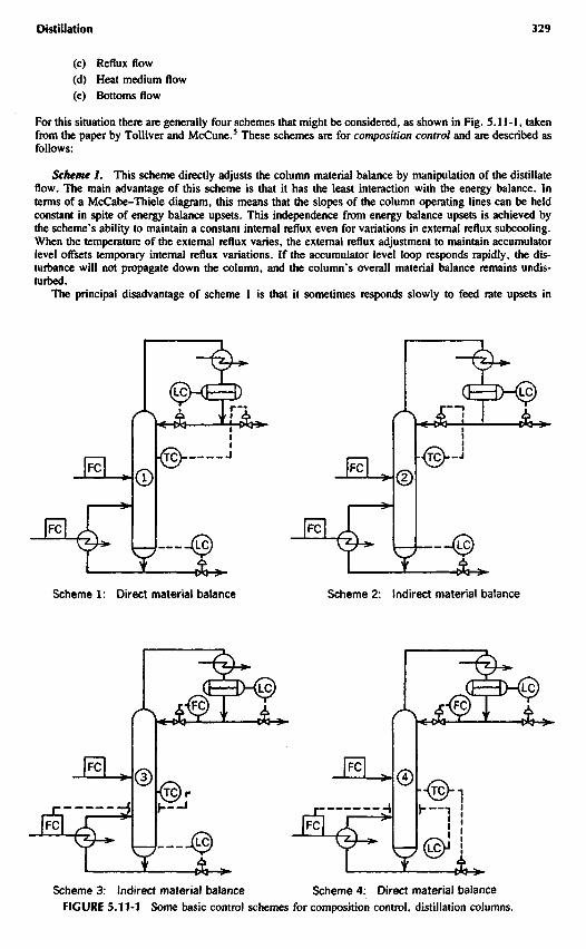
For this situation there are generally four schemes that might be considered, as shown in Fig. 5.11-1, takenfrom the paper by Tolliver and McCune.5 These schemes are for composition control and are described asfollows:

Scheme 1. This scheme directly adjusts the column material balance by manipulation of the distillateflow. The main advantage of this scheme is that it has the least interaction with the energy balance. Interms of a McCabe-Thiele diagram, this means that the slopes of the column operating lines can be heldconstant in spite of energy balance upsets. This independence from energy balance upsets is achieved bythe scheme's ability to maintain a constant internal reflux even for variations in external reflux subcooling.When the temperature of the external reflux varies, the external reflux adjustment to maintain accumulatorlevel offsets temporary internal reflux variations. If the accumulator level loop responds rapidly, the dis-turbance will not propagate down the column, and the column's overall material balance remains undis-turbed.

The principal disadvantage of scheme 1 is that it sometimes responds slowly to feed rate upsets in

Scheme 1: Direct material balance Scheme 2: Indirect material balance

Scheme 3: Indirect material balance Scheme 4: Direct material balance

FIGURE 5.11-1 Some basic control schemes for composition control, distillation columns.

stripping columns where the column objectives strongly emphasize control of bottom product composition.Also, in columns with relatively large accumulator holdup, often found in pilot plant columns, the levelcontrol (within the composition loop) can be too slow for effective composition control. Scheme 1 shouldbe selected whenever the distillate flow is one of the smaller flows in the column. If column dynamicsfavor other schemes, but the guidelines do not, then additional feed-forward controls may be applied tothis scheme to improve the dynamics.

Scheme 2. This scheme indirectly adjusts the material balance through the two level control loops.This arrangement has the advantage of reducing the ratio of effective dead time to total lag time within thecomposition loop. It has the disadvantage of allowing greater interaction between the material and energybalances because internal reflux is not held constant. This scheme should be considered when the reflux issmaller than other flows in the column and when the reflux to distillate ratio is 0.8 or less. It should alsobe considered for applications where reducing the ratio of effective dead time to total lag time in thecomposition loop is a significant and necessary consideration.

Scheme 3. This scheme is a common arrangement in the chemical industry, used primarily on strippingcolumns. This arrangement indirectly adjusts the material balance in the same manner as scheme 2. It hasthe advantage of offering the minimum effective dead time to total lag time in the composition loop. It hasthe disadvantage of having the greatest interaction between the material and energy balances. Because thereboiler is this interaction, scheme 3 is not recommended in columns where the reboiler boilup to columnfeed ratio is 2.0 or greater.

Scheme 4. This scheme directly manipulates the material balance by adjusting the bottom productflow. This scheme has the advantage of little interaction between the material and energy balances, similarto scheme 1. However, the sump level loop can significantly increase the ratio of effective dead time tototal lag time in the composition loop. Furthermore, the sump level loop is often subject to an inverseresponse, which can make the loop difficult to implement or even impossible to control. Because of thesedifficulties, this arrangement is recommended only when the bottom product flow is significantly smallerthan other flows in the column and is less than 20% of the boilup from the reboiler.

The authors point out that the schemes shown in Fig. 5.11-1 are conceptual arrangements and the readeris cautioned against inferring any control hardware requirements from such simplified diagrams.

In Fig. 5.11-1, composition of a flowing stream in the column is inferred from its temperature. Thisis the most common inferential measurement of composition; others include density, refractive index,viscosity and thermal conductivity. In some cases, especially for fractionating close-boiling mixtures, directcomposition measurement by stream analyzer may be desired. The most common analyzer used is the gaschromatograph, although other techniques such as mass spectrometry may be used in some instances. Thelocation of the point of measurement is determined by the gradient of composition or by column dynamicconsiderations.

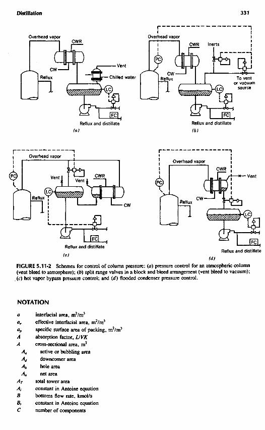
For column pressure control there are three general approaches: vent bleed (to atmosphere or to vacuumsystem), hot vapor bypass, and flooded condenser. These approaches are illustrated in Fig. 5.11-2.5 Foran atmospheric column, the vent approach is quite simple. The vapor bypass represents a temperatureblending method. Partial flooding of the condenser surface adjusts the heat transfer capability of thecondenser. The schemes are generally self-explanatory.

Distillation control schemes may be analyzed either on a steady-state (sensitivity analysis) or on adynamic basis. The latter requires a dynamic model that takes into account the dynamic response of thecolumn and the control loops. An example of a dynamic model is described by McCune and Gallier,6 butit should be apparent from the material presented earlier that the holdup characteristics of distillation columndevices can vary widely, and such variation should be accommodated by the model. The development ofthe new high-efficiency packings has caused a new look at the system dynamics when the liquid holdup inthe column is quite low, and thus the existing models for trays may not be adjustable to application topackings. The use of a tray-type dynamic model is described in the article by Gallier and McCune;7 nowork to date has been reported for packed column dynamic models.

Steady-state analysis is based on the determination of a new set of operating conditions that would berequired by an imposed upset of the system. In this case there is the constraint of a fixed number of traysor stages in the column, and the assumption is often possible that there would be no significant change inefficiency caused by the upset. Thus, in a simplistic example, one could modify a McCabe-Thiele plot toaccommodate a changed feed composition, by trial-and-error, finding a new set of operating lines thatwould not change the required theoretical stages. The steady-state approach, called "sensitivity analysis,"determines the new set of operating conditions but says nothing about how long it takes to reach the newstate—nor does it say anything about the gyrations that might occur during the period of transition. Still,it should always be carried out for new column designs.

Reflux and distillateReflux and distillate

FIGURE 5.11-2 Schemes for control of column pressure: (a) pressure control for an atmospheric column(vent bleed to atmosphere); (b) split range valves in a block and bleed arrangement (vent bleed to vacuum);(c) hot vapor bypass pressure control; and (d) flooded condenser pressure control.

NOTATION

interfacial area, m2/m3

effective interfacial area, m2/m3

specific surface area of packing, m2/m3

absorption factor, LI VKcross-sectional area, m2

active or bubbling areadowncomer areahole areanet area

total tower areaconstant in Antoine equationbottoms flow rate, kmol/sconstant in Antoine equationnumber of components

VentVent

CWReflux

Reflux C W

VentCWR

Overhead vaporOverhead vapor

CWR

Overhead vaporCWR

iOverhead vapor

CWR lnerts

CWReflux

CW-Reflux

Vent

Chilled water To ventor vacuum

source

Reflux and distillate(a)

Reflux and distillate(b)

constant in Eq. (5.7-26)drag coefficient, dimensionlessconstant in Antoine equationcapacity (Souders-Brown) coefficient based on net area, m/scapacity coefficient at flood, m/scapacity coefficient based on active area, m/s

discharge (orifice) coefficient, dimensionlesscapillary number, dimensionlesscooling waterequivalent diameter of packing, mmhole diameter, mmdiameter of random packing element, mmdiameter of liquid droplet, mmliquid diffusion coefficient, m2/svapor diffusion coefficient, m2/seddy diffusion coefficient, m2/sefficiency, fractional

efficiency, corrected for entrainmentMurphree vapor efficiencyoverall column efficiencypoint (local) efficiency, vapor basis

exponentialentrainment rate, moles/timefriction factor, dimensionlessvapor flow F factor, Uvp

m, m/s (kg/m3)1'2

F factor through active areaF factor through hole areaF factor through total tower cross-sectional area

molar flow rate of feed to stage n, kmol/spacking factor, mFroude number, dimensionlessgravitational constant, 9.81 m/s2

conversion factor, 32.2 lbm/lbf (ft/s2); not used with SI system

vapor mass velocity, kg/s-m2

molar velocity of vapor, kmol/s • m2

liquid enthalpy, J/kghead, mm liquid (pressure loss)pressure loss through holespressure loss under downcomer apronpressure loss for flow through distributorresidual pressure loss

total pressure drop across trayheight of liquid in downcomer, mmequivalent height of liquid holdup on tray, mm liquidcrest of liquid over weir, mmweir height, mmenthalpy of vapor, J/kgheight of a transfer unit (HTU), m

height of a liquid-phase transfer unitheight of an overall liquid transfer unitheight of an overall vapor transfer unitheight of a vapor transfer unit

liquid holdup, volume fractionoperating holdupstatic holduptotal holdup

height equivalent to a theoretical plate, mliquid holdup on tray, kg*molesindividual-phase mass transfer coefficient, m/s or kmol/(s*m2-mole fraction)vapor-phase coefficientliquid-phase coefficientoverall mass transfer coefficient, m/s or kmol/(s*m2*mole fraction)

overall coefficient based on vapor concentrationoverall coefficient based on liquid concentrations

vapor-liquid equilibrium ratiocomponent molar flow rate, kmol/sweir length, mm or mmolar liquid rate, kmol/smolar liquid rate in stripping section, kmol/smolar liquid velocity, kmol/s-m2

liquid rate, m3/s • m weirslope of the equilibrium linestage designation, stripping sectionstage designation, rectifying section (or general)top stagenumber of transfer unitsnumber of liquid transfer unitsnumber of overall transfer units, liquid concentration basisnumber of overall transfer units, vapor concentration basisnumber of vapor transfer unitsmolar flux of species A, kmol/s *mnumber of actual traysnumber of theoretical stagesminimum number of theoretical stagesvapor pressure, mm Hgpartial pressure, mm Hgtotal pressure, mm HgPoynting correction [Eq. (5.2-3)]Peclet number, dimensionlessheat ratio [Eq. (5.3-19)]volumetric flow rate of liquid, m3/sheat flow, J/s

flow to reboilerflow from condenserflow to or from stage n

volume of froth, m3

volumetric flow rate of vapor, m3/sgas constantreflux ratiominimum reflux ratio (also Rm)Reynolds number, dimensionlessnumber of mixing stages on traynumber of moles in stillpotSchmidt number, dimensionlessSherwood number dimensionless

time, stemperature, Ktray spacing, mmliquid velocity, m/svelocity under downcomer apron, m/svapor velocity, m/s

velocity through active areavelocity through hole areavelocity through net areaflooding velocity through net areasuperficial velocity (also Us)

liquid velocity, m/seffective vapor velocity, m/ssuperficial vapor velocity in packed column, m/smolar volume, m3/kmolpartial molar volume, mVkmolcomponent vapor flow rate, kmol/smolar flow rate of vapor, kmol/srate of sidestream vapor withdrawal from tray nmolar flow rate of liquid in stripping section, moles/timeliquid flow rate across tray [Eq. (5.9-25)], nrVs-mlength of liquid flow path, mmole fraction in liquidmole fraction in vaporequilibrium mole fraction in vapormole fraction in feedheight of packing, mfroth height on tray, m

Subscripts

active area basisfeedheavy keycomponent /component./liquidlight keystage noperatingstillpotsteady statetime /vaporinitial time (time 0)components 1 and 2stages 1 and 2

Superscripts

liquidvapor

Greek Letters

a relative volatilitya average relative volatility/3 aeration factory activity coefficientF liquid flow rate, based on length, nrVs-mA hydraulic gradient, mm liquidA difference point, Ponchon-Savarit methodAp pressure drop, mm liquidAp0 pressure drop through dry bed of packing€ void fraction or froth porosity$ angle of inclination of channel in structured packing6 notch angle, degrees9 exposure time, sX ratio of slope of equilibrium line to that of operating linep, viscosity, kg/m-sT 3.1416p density, kg/ma surface tension, mN/m (dynes/cm)<f> parameter for packed column mass transfer, Eq. (5.10-8)<ff geometric packing factor, Eq. (5.8-16)<f>e effective froth density, dimensionless4>i fugacity coefficient, dimensionless<£, fugacity coefficient for i in mixture^f1 fugacity coefficient for pure /, at system temperature and pressure equal to the vapor pressure of /

ty froth density, dimensionlessX aperature correction factor, Eq. (5.8-16)>f/ parameter for packed column mass transfer, Eq. (5.10-7)^ ratio, density of liquid to density of water

REFERENCES

Section 5.2

5.2-1 J. H. Hildebrand, J. M. Prausnitz, and R. L. Scott, Regular and Related Solutions, Van Nostrand

Reinhold, New York, 1970.5.2-2 R. C. Reid, J. M. Prausnitz, and T. K. Sherwood, The Properties of Gases and Liquids, 3rd ed.,

McGraw-Hill, New York, 1977.5.2-3 H. H. Y. Chien and H. R. Null, AIChEJ., 18, 1177 (1972).5.2-4 E. HaIa, J. Pick, V. Fried, and O. Vilim, Vapor-Liquid Equilibrium, 2nd ed., Pergamon, Oxford,

1967.5.2-5 E. HaIa, I. Wichterle, J. Polak, and T. Boublik, Vapor-Uquid Equilibrium at Normal Pressures,

Pergamon, Oxford, 1968.5.2-6 I. Wichterle, J. Linek, and E. HaIa, Vapor-Liquid Equilibrium Data Bibliography, Elsevier,

Amsterdam, 1975.5.2-7 J. C. Chu, S. L. Wang, S. L. Levy, and R. Paul, Vapor-Liquid Equilibrium Data, J. B. Edwards,

Ann Arbor, 1956.5.2-8 M. Hirata, S. Ohe, and K. Nagahama, Computer Aided Data Book of Vapor-Liquid Equilibria,

Elsevier, Amsterdam, 1975.5.2-9 J. Gmehling, U. Onken, and W. ArIt, Vapor-Liquid Equilibrium Collection (continuing series),

DECHEMA, Frankfurt, 1979.5.2-10 Chemshare Corp., Houston, Texas.5.2-11 S. T. Hadden and H. G. Grayson, Petrol. Refiner, 40(9), 207 (1961).5.2-12 Natural Gas Processors Suppliers Assn., Engineering Data Book, 9th ed., Tulsa, 1972.

5.2-13 L. H. Horsley, Azeotropic Data—III, American Chemical Society Advances in Chemistry Series116, Washington, DC, 1973.

Section 5.3

5.3-1 W. L. McCabe and E. W. Thiele, Ind. Eng. Chem., 17, 605 (1925).5.3-2 M. Ponchon, Tech. Mod., 13, 20, 55 (1921).5.3-3 R. Savarit, Arts Metiers, 65, 142, 178, 241, 266, 307 (1922).5.3-4 W. L. McCabe and J. C. Smith, Unit Operations of Chemical Engineering, 3rd ed., McGraw-

Hill, New York, 1976.5.3-5 M. R. Fenske, Ind. Eng. Chem., 24, 482 (1932).5.3-6 A. J. V. Underwood, Chem. Eng. Prog., 44, 603 (1948).5.3-7 H. H. Chien, Chem. Eng. ScL, 28, 1967 (1973).5.3-8 H. H. Chien, AIChE J., 24, 606 (1978).5.3-9 W. K. Lewis and G. L. Matheson, Ind. Eng. Chem., 24, 494 (1932).5.3-10 C D . Holland, Fundamentals of Multicomponent Distillation, McGraw-Hill, New York, 1981.5.3-11 E. W. Thiele and R. L. Geddes, Ind. Eng. Chem., 25, 290 (1933).5.3-12 N. R. Amundson and A. J. Pontinen, Ind. Eng. Chem., 50, 730 (1958).5.3-13 J. R. Friday and B. D. Smith, AIChEJ., 10, 698 (1964).5.3-14 J. C. Wang and G. E. Henke, Hydrocarbon Proc, 45(8), 155 (1966).5.3-15 J. C. Wang and Y. L. Wang, A Review on the Modeling and Simulation of Multistaged Separation

Processes, in Foundations of Computer-Aided Chemical Process Design, Vol. 2, R. S. H. Manand W. D. Seider (Eds.), American Institute of Chemical Engineers, New York, 1981.

5.3-16 E. R. Gilliland, Ind. Eng. Chem., 32, 1220 (1940).5.3-17 H. E. Eduljee, Hydrocarbon Proc, 54(9), 120 (1975).5.3-18 J. H. Erbar and R. N. Maddox, Petrol. Ref, 40(5), 183 (1961).5.3-19 E. R. Gilliland, Ind. Eng. Chem., 32, 918 (1940).5.3-20 J. R. Fair and W. L. Bolles, Chem. Eng., 75(9), 156 (Apr. 22, 1968).

Section 5.5

5.5-1 L. H. Horsley, Azeotropic Data—III, American Chemical Society Advances in Chemistry No.116, Washington, DC, 1973.

5.5-2 M. Lecat, Tables azeotropiques, 1'Auteur, Brussels, 1949.5.5-3 H. Renon and J. M. Prausnitz, AIChEJ., 14, 135 (1968).5.5-4 C. S. Robinson and E. R. Gilliland, Elements of Fractional Distillation, 4th ed., McGraw-Hill,

New York, 1950.5.5-5 B. T. Brown, H. A. Clay, and J. M. Miles, Chem. Eng. Prog., 66(8), 54 (1970).5.5-6 B. K. Kruelski, C C . Herron, and J. R. Fair, "Hydrodynamics and Mass Transfer on Three-

Phase Distillation Trays," presented at Denver AIChE Meeting, Aug. 1983.5.5-7 E. J. Hoffman, Azeotropic and Extractive Distillation, Interscience, New York, 1964.5.5-8 C Black, R. A. Golding, and D. E. Ditsler, Azeotropic Distillation Results from Automatic

Computer Calculations, in Extractive and Azeotropic Distillation, Chap. 5, American ChemicalSociety Advances in Chemistry No. 115, Washington, DC, 1972.

5.5-9 J. A. Gerster, Chem. Eng. Prog., 65(9), 43 (1969).5.5-10 C Black and D. E. Ditsler, Dehydration of Aqueous Ethanol Mixtures by Extractive Distillation,

in Extractive and Azeotropic Distillation, Chap. I, American Chemical Society Advances in Chem-istry No. 115, Washington, DC, 1972.

5.5-11 L. Berg, Chem. Eng. Prog., 65(9), 52 (1969).5.5-12 R. H. Ewell, J. M. Harrison, and C Berg, Ind. Eng. Chem., 36, 871 (1944).5.5-13 H. G. Drickamer, G. G. Brown, and R. R. White, Trans. AIChE, 41, 555 (1945).5.5-14 H. G. Drickamer and H. H. Hummel, Trans. AlChE, 41, 607 (1945).5.5-15 B. D. Smith, Design of Equilibrium Stage Processes, McGraw-Hill, New York, 1963.5.5-16 R. Kumar, J. M. Prausnitz, and C J . King, Process Design Considerations for Extractive Distil-

lation: Separation of Propylene-Propane, in Extractive and Azeotropic Distillation, Chap. 2, Amer-ican Chemical Society Advances in Chemistry No. 115, Washington, DC, 1972.

5.5-17 J. A. Gerster, T. Mizushina, T. N. Marks, and A. W. Catanach, AJChE J., 1, 536 (1955).5.5-18 E. R. Hafslund, Chem. Eng. Prog., 65(9), 58 (1969).5.5-19 R. R. Bannister and E. Buck, Chem. Eng. Prog., 65(9), 65 (1969).5.5-20 D. P. Tassios, Rapid Screening of Extractive Distillation Solvents. Predictive and Experimental

Techniques, in Extractive and Azeotropic Distillation, Chap. 4, American Chemical Society Ad-vances in Chemistry Series No. 115, Washington, DC, 1972.

5.5-21 J. Drew and M. Probst (Eds.), Tall Oil, Pulp Chemicals Assn., New York, 1981.5.5-22 J. W. Packie, Trans. AIChE, 37, 51 (1941).5.5-23 G. S. Houghland, E. J. Lemieux and W. C. Schreiner, Oil Gas J., 52, 198 (July 26, 1954).5.5-24 M. W. Van Winkle, Distillation, McGraw-Hill, New York, 1967.5.5-25 R. R. Dreisbach, Pressure-Volume-Temperature Relationships of Organic Compounds, Handbook

Publishers, Cleveland, 1952.5.5-26 M. J. P. Bogart, Trans. AIChE, 33, 139 (1937).5.5-27 R. F. Jackson and R. L. Pigford, Ind. Eng. Chem., 48, 1020 (1932).5.5-28 C. D. Holland and A. I. Liapis, Computer Methods for Solving Dynamic Separation Problems,

McGraw-Hill, New York, 1983.5.5-29 E. L. Meadows, Chem. Eng. Prog. Symp. Ser. No. 46, 59, 48-55 (1963).5.5-30 G. P. Distefano, AIChEJ., 14, 190 (1968).5.5-31 J. F. Boston, H. I. Britt, S. Jirapongphan, and V. B. Shah, An Advanced System for the Simulation

of Batch Distillation Operations, in Foundations of Computer-Aided Chemical Process Design,Vol. 2, American Institute of Chemical Engineers, New York, 1981.

Section 5.6

5.6-1 R. Krishnamurthy and R. Taylor, Ind. Eng. Chem. Proc. Des. Dev., 24, 513 (1985).

Section 5.7

5.7-1 American Institute of Chemical Engineers, Bubble-Tray Design Manual, New York, 1958.5.7-2 D. L. Bennett, R. Agrawal, and P. J. Cook, AIChEJ., 29, 434 (1983).5.7-3 P. A. M. Hofhuis and F. J. Zuiderweg, Int. Chem. Eng. Symp. Ser., 56, 2.2/1 (1979).5.7-4 R. E. Loon, W. V. Pincewski, and C. J. D. Fell, Trans. Inst. Chem. Eng., 51, 374 (1974).5.7-5 M. Souders and G. G. Brown, Ind. Eng. Chem., 26, 98 (1934).5.7-6 F. C. Silvey and G. J. Keller, Chem. Eng. Prog., 62(1), 69 (1966).5.7-7 J. R. Fair, Petro/Chem. Eng., 33(10), 45 (1961).5.7-8 E. Kirschbaum, Distillier-und Rektifiziertechnik, 4th ed., Springer Verlag, Berlin, 1969.5.7-9 J. R. Fair, Distillation in Practice, course notes for Today course, American Institute of Chemical

Engineers, New York, 1981.5.7-10 J. R. Fair and R. L. Matthews, Petrol. Ref, 37(4), 153 (1958).5.7-11 T. Yanagi, "Performance of Trays in Low Liquid Rate Fractionation," motion picture shown at

AIChE Miami meeting, Nov. 1978 (film available from Fractionation Research, Inc.)5.7-12 A. P. Colburn, Ind. Eng. Chem., 28, 526 (1936).5.7-13 J. R. Fair, Chap. 15 in B. D. Smith (Ed.), Design of Equilibrium Stage Processes, McGraw-Hill,

New York, 1963.5.7-14 S. Zanelli and R. Del Bianco, Chem. Eng. J., 6, 181 (1973).5.7-15 I. Leibson, R. E. Kelley, and L. A. Bullington, Petrol. Ref, 36(2), 127 (1957).5.7-16 M. H. Hutchinson, A. G. Buron and B. P. Miller, Paper presented at AIChE meeting, Los

Angeles, May 1949.5.7-17 W. L. Bolles and J. R. Fair, Distillation, Vol. 16 of Encyclopedia of Chemical Processing and

Design, J. J. McKetta (Ed.), Marcel Dekker, New York, 1982.5.7-18 W. L. Bolles, Chap. 14 in B. D. Smith (Ed.), Design of Equilibrium Stage Processes, McGraw-

Hill, New York, 1963.5.7-19 R. Billet, S. Conrad, and C. M. Grubb, Int. Chem. Eng. Symp. Ser. No. 32, 5, 111 (1969).5.7-20 P. J. Hoek and F. J. Zuiderweg, AIChEJ., 28, 535 (1982).5.7-21 Glitsch, Inc., Ballast Tray Design Manual, Bulletin 4900, Dallas, Texas, 1961.

Section 5.8

5.8-1 G. K. Chen, Chem. Eng., 91(5), 40 (Mar. 5, 1984).5.8-2 D. F. Stedman, Trans. AlChE, 33, 153 (1937).5.8-3 L. B. Bragg, Trans. AIChE1 37, 19 (1941).5.8-4 A. J. Hayter, lnd. Chemist, 59 (Feb. 1952).5.8-5 R. C. Scofield, Chem. Eng. Prog., 46, 405 (1950).5.8-6 L. B. Bragg, lnd. Eng. Chem., 49, 1062 (1957).5.8-7 R. Billet, Int. Chem. Eng. Symp. Ser. No. 32, 4, 42 (1969).5.8-8 M. Huber, U.S. Patent 3,285,587 (Nov. 15, 1966).5.8-9 J. R. Fair, Chem. Eng. Prog., 66(3), 45 (1970).5.8-10 T. Baker, T. H. Chilton, and H. C. Vernon, Trans. AIChE, 31, 296 (1935).5.8-11 F. C. Silvey and G. J. Keller, Int. Chem. Eng. Symp. Ser. No. 32, 4, 18 (1969).5.8-12 M. A. Albright, Hydrocarbon Proc, 63(9), 173 (1984).5.8-13 J. G. Kunesh, L. L. Lahm, and T. Yanagi, "Liquid Distribution Studies in Packed Beds"

presented at Chicago AIChE Meeting, Nov. 1985.5.8-14 H. L. Shulman, C. F. Ullrich, and N. Wells, AIChEJ., 1, 247, 253 (1955).5.8-15 J. E. Buchanan, lnd. Eng. Chem. Fundam., 6, 400 (1967).5.8-16 J. L. Bravo and J. R. Fair, lnd. Eng. Chem. Proc. Des. Dev., 21, 162 (1982).5.8-17 B. R. Sarchet, Trans. AlChE, 38, 283 (1942).5.8-18 F. C. Silvey and G. J. Keller. Chem. Eng. Prog., 62(1), 69 (1966).5.8-19 T. K. Sherwood, G. H. Shipley, and F. A. L. Holloway, lnd. Eng. Chem., 30, 765 (1938).5.8-20 J. S. Eckert, Chem. Eng. Prog., 66(3), 39 (1970).5.8-21 J. E. Buchanan, lnd. Eng. Chem. Fundam., 8, 502 (1969).5.8-22 G. G. Bemer and G. A. J. Kallis, Trans, lnst. Chem. Eng., 56, 200 (1978).5.8-23 R. Billet and J. Mackowiak, Fette-Seifen-Anstrichmittel. 86, 349 (1984).5.8-24 J. L. Bravo, J. A. Rocha, and J. R. Fair, Hydrocarbon Proc, 65(3), 45 (1986).5.8-25 W. L. Bolles and J. R. Fair, Distillation in Practice, Notes for American Institute of Chemical

Engineers course, New York, 1984.

Section 5.9

5.9-1 H. E. O'Connell, Trans AIChE, 42, 741 (1946).

5.9-2 J. R. Fair, W. L. Bolles, and H. R. Null, lnd. Eng. Chem. Proc. Des. Dev., 22, 53 (1983).5.9-3 R. L. Geddes, Trans. AIChE, 42, 79 (1946).5.9-4 AIChE [American Institute of Chemical Engineers], Bubble Tray Design Manual, New York,

1958.5.9-5 A. S. Foss and J. A. Gerster, Chem. Eng. Prog., 52, 28 (1956).5.9-6 H. Chan and J. R. Fair, lnd. Eng. Chem. Proc. Des. Dev., 23, 814 (1984).5.9-7 D. A. Diener, lnd. Eng. Chem. Proc. Des. Dev., 6, 499 (1967).5.9-8 W. K. Lewis, Jr., lnd. Eng. Chem., 28, 399 (1936).5.9-9 M. F. Gautreaux and H. E. O'Connell, Chem. Eng. Prog., 51, 232 (1955).5.9-10 P. E. Barker and M. F. Self, Chem. Eng. Sci., 17, 541 (1962).5.9-11 K. E. Porter, M. J. Lockett, and C. T. Lim, Trans, lnst. Chem. Eng., 50, 91 (1972).5.9-12 R. J. Bell, AlChE / . , 18, 498 (1972).5.9-13 G. G. Young and J. H. Weber, lnd. Eng. Chem. Proc. Des. Dev., 11, 440 (1972).5.9-14 R. Krishna, H. F. Martinez, R. Sreedhar, and G. L. Standart, Trans, lnst. Chem. Eng., 55, 178

(1977).5.9-15 H. Chan and J. R. Fair, lnd. Eng. Chem. Proc. Des. Dev., 23, 820 (1984).5.9-16 H. L. Toor and J. K. Burchard, AlChE J., 6, 202 (1960).Section 5.105.10-1 W. A. Peters, J. lnd. Eng. Chem., 14, 476 (1922).5.10-2 J. S. Eckert, E. H. Foote, L. R. Rollison, and L. F. Walter, lnd. Eng. Chem., 59(2), 41 (1967).

5.10-3 D. Cornell, W. G. Knapp, and J. R. Fair, Chem. Eng. Prog., 56(7), 68 (1960).5.10-4 K. Onda, H. Takeuchi, and Y. Okumoto, J. Chem. Eng. Japan, 1, 56 (1968).5.10-5 J. L. Bravo and J. R. Fair, lnd. Eng. Chem. Proc. Des. Dev., 21, 162 (1982).5.10-6 W. L. Bolles and J. R. Fair, Int. Chem. Eng. Symp. Ser. No. 56, 3.3/35 (1979).5.10-7 W. L. Bolles and J. R. Fair, Chem. Eng., 89(14), 109 (July 12, 1982).5.10-8 J. L. Bravo, J. A. Rocha, and J. R. Fair, Hydrocarbon Proc, 64(1), 91 (1985).5.10-9 H. F. Johnstone and R. L. Pigford, Trans. AlChE, 38, 25 (1942).

Section 5.11

5.11-1 A. E. Nisenfeld and R. C. Seeman, Distillation Columns, Instrument Society of America (ISA),Research Triangle Park, NC, 1981.

5.11-2 F. G. Shinskey, Distillation Control, 2nd ed., McGraw-Hill, New York, 1984.5.11-3 P. B. Deshpande, Distillation Dynamics and Control, Instrument Society of America (ISA), Re-

search Triangle Park, NC, 1984.5.11-4 P. S. Buckley, W. L. Luyben, and J. P. Shunta, Design of Distillation Control Systems, Instrument

Society of America (ISA), Research Triangle Park, NC, 1985.5.11-5 T. L. Tolliver and L. C. McCune ISA Transactions, 17(3), 3 (1978).5.11-6 L. C. McCune and P. W. Gallier, ISA Transactions, 12(3), 193 (1973).5.11-7 P. W. Gallier and L. C. McCune, Chem. Eng. Prog., 70(9), 71 (1974).