Embed Size (px)
Citation preview

APPLIED & INTERDISCIPLINARY MATHEMATICS | RESEARCH ARTICLE
Prevention strategy for superinfectionmathematical model tuberculosis and HIVassociated with AIDSMuhammad Tahir1*, Syed Inayat Ali Shah1 and Gul Zaman2
Abstract: In this article, we extended the co-infection mathematical model [1] foroptimal control purpose. We initially derived a threshold number R0 and found
bounded and biological region for the study of the proposed model. Here, wedeveloped a methodology through the considered superinfection problem which isgetting abate while neglecting Acquired Immuno deficiency Syndrome (AIDS)because it is a noncurable disease. For this, we developed the following controlvariables in our model: V1, using treatment against TB; V2, infection control in
health-care center; V3, co-treatment of multidrug-resistant TB and HIV or start bothHIV antiretroviral and anti-TB drug therapy; and V4, avoid close contact with TBpatient. These are defined with some different schemes to minimize and control theinfection from any community and population. In the last section, numericalsimulation is presented which supports the given model.
Subjects: Science; Biology; Mathematics & Statistics; Applied Mathematics; MathematicalBiology; Cancer; ChronicDiseases
Keywords: mathematical model; threshold number; sensitivity analysis; biological region;optimal control; TB/HIV/AIDS; numerical simulation
ABOUT THE AUTHORSMuhammad Tahir is the corresponding authorof this research article. His areas of researchare Mathematical Biology and Fluid Dynamics.He is affiliated with Department ofMathematics, Islamia College, UniversityPeshawar, 25000 Pakistan. E-mail: [email protected]; Tel: +92-345-9063508
Syed Inayat Ali Shah is currently working asa professor and dean in Mathematics atIslamia College University Peshawar, 25000Pakistan. He has obtained his Ph.D. degreefrom Saga University, Japan, in 2002. E-mail:[email protected]
Gul Zaman is currently working as a vicechancellor at University of Malakand, lower Dir,18800 Chakdara, Pakistan. He has obtained hisPh.D. from Pusan National University, SouthKorea, in 2008. E-mail: [email protected]
PUBLIC INTEREST STATEMENTIn this study we discussed the three acting playdiseases AIDS/HIV/TB. Tuberculosis (TB) is apotentially serious infectious disease which bringHIV and then AIDS if no treatment taken. Here allthe diseases are so harmful and transmissible,even if an individual get infection it transmit andcirculate in the entire world. In this study weshown that vaccination is key factor against thesediseases. The study is valuable for all mankindto avoid from these virus need to adopt good andhealthy environment, isolation from infectedindividuals, vaccination at proper time etc. Thestudy also provide a wide range of safety if pre-caution are adopted in advance, and if infectedshould be treated on time, is the necessary advisefor all mankind.
Tahir et al., Cogent Mathematics & Statistics (2019), 6: 1637166https://doi.org/10.1080/25742558.2019.1637166
© 2019 The Author(s). This open access article is distributed under a Creative CommonsAttribution (CC-BY) 4.0 license..
Received: 24 January 2019Accepted: 23 June 2019First Published: 28 June 2019
*Corresponding author: MuhammadTahir, Department of Mathematics,Islamia College, Peshawar, KPK25000, PakistanE-mail: [email protected]
Reviewing editor:Yuriy Rogovchenko, Universitetet iAgder, Norway
Additional information is available atthe end of the article
Page 1 of 17

1. Introduction and related literatureMathematical models have a great role in science field. Developing a mathematical model istermed mathematical modeling which is used in natural sciences such as physics, chemistry,and biology, as well as in engineering sciences such as computer sciences and electrical sciences.It is the art to transfer any problems from application area into tractable mathematical formula-tion. Developing a mathematical models is the process that uses maths to represent, analyze,make predictions, or otherwise provide insight into the real-world phenomena. There are manymathematical models and many techniques to solve a particular problem. Mathematical biologycan help us solve massive problems such as recycling option or the spread of a disease ina population. Work in mathematical biology is typically a collaboration between mathematicianand biologist. Similarly, control of an infectious disease is obligatory; therefore, some mathema-tical models and methodology are adopted to control infection. This is known as optimal control.
1.1. AIDS/HIV/TBAIDS is also called acquired immune deficiency syndrome which is occurred by a condition calledspectrum. In the initial stage, AIDS patients show no clear symptoms or influenza-like illness(International Committee on Taxonomy of Viruses, 2002b). The most important fact about AIDSis that it takes a long time period for symptoms to be obvious (HIV/AIDS Fact sheet N360, 2015).While the late symptoms brought a viral infection called Acquired Immunodeficiency Syndrome(AIDS) (HIV/AIDS Fact sheet N360, 2015). AIDS can be spread by unprotected sex, blood transfu-sion, and usable syringes and from mother to child during pregnancy and breastfeeding which arethe two major ways (About HIV/AIDS, 2015). Nowadays AIDS has no proper cure; however,antiretroviral vaccines have been developed which have a low infection rate, thus enabling AIDSpatients to possess a near-normal life (Cunningham, Donaghy, Harman, Kim, & Turville, 2010). Thetotal survival time without treatment for AIDS individual is 11 years after infection (Markowitz,edited by William N. Rom; associate editor, Steven B, 2007). Approximately 36.7 million individualsare living with HIV infection, while 1 million deaths occurr according to a survey conducted in 2016(UNAIDS, WHO, 2007), and these infected people mostly live in sub-Saharan Africa (UNAIDS, WHO,2007). Then, according to a 2014 survey, AIDS caused an estimated 39 million deaths worldwide(Fact sheet—Latest statistics on the status of the AIDS epidemic | UNAIDS, 2017). Initial infectionwith HIV is called acute HIV syndrome (Basic Statistics, 2015), while the next stage is called clinicallatency. Without treatment in the second stage of HIV, the survival time is considered to be 3–20years (Evian, 2006; xxxxx, 2007). The third chronic and last stage is called AIDS which can bedefined as when the CD4 + T cells go down below 200 cells per µL (Duoyi, 2001). A recent studyabout AIDS was presented by Win Min Han et al. on 27 September 2018 which was related to CD4and CD8 cell normalization and Tahir et al. presented a coinfection model (Tahir, Shah, & Zaman,2018; Win Min et al., 2018). Optimal control theory is one of the powerful tools used inmathematics to control or reduce infection in the community and population. In this situation,a control law is required through which we judge the problem and minimize the infection.
Human immunodeficiency virus is a global health problem which is a lentivirus and causes HIVinfection. It is one of the most studied infectious diseases in the world. If an infected individualdoes not use medicines against HIV, then the total survival time of that individualis 9–11 years(Lawn & Zumla, 2011). HIV is differentiated into two forms: HIV-1 and HIV-2. HIV-1 virus whichwas initially discovered is considered that mostly infect HIV globally (Doitsh et al., 2014).Transmission rate of HIV-2 mainly occurred in West Africa (International Committee onTaxonomy of Viruses, 2002a). A recent work on optimal control in 2018 has been done byTahir el.al who presented the stability and optimal control of Middle East respiratory syn-drome corona virus (MERS-CoV) (Tahir et al., 2018). HIV destroyed the system of basic immunecells of the human body system, like helper T cells (UNAIDS, WHO, 2007), and it decreases thenumbers of CD4 + T cells by a mechanism called pyroptosis and broadly infects T-cell apoptosisof uninfected cells of the body (UNAIDS, WHO, 2007). When CD4 + T cells of a person decreasebelow the critical numbers, the body is prone infections (Cunningham et al., 2010). An optimalcontrol was presented by Adams et al. HIV dynamics modeling, data analysis, and optimal
Tahir et al., Cogent Mathematics & Statistics (2019), 6: 1637166https://doi.org/10.1080/25742558.2019.1637166
Page 2 of 17

treatment protocols (Duoyi, 2001) were discussed. Also for the optimal control purposes Hem RajJoshi et al. discussed the optimal control of an HIV immunology model (Evian, 2006). Recently,Ciaranello et al. presented simulation modeling and metamodeling to explain national andinternational HIV policies for children and adolescents (WHO, 2007).
Tuberculosis (TB) is an infectious disease usually caused by the bacterium Mycobacterium tuber-culosis (Tahir & Shah, 0000) and simply known as a contagious infection. TBgenerally affects thelungs. Most TB patients show no symptoms, and this is known as latent TB. Latent TB individuals arenot harmful to people and do not spread the infection further. A tool to diagnose latent TB such asthe tuberculin skin test (TST) is used. Nowadays, most TB cases are considered curable by the use ofantibiotics. The latent infections progress into active TB in about 10% of the cases. Symptoms for theactive TB include feeling of sickness, weight loss, high fever, cough, chest pain, and chronic coughcontaining blood or sputum. Medicines are prescribed for a period of 6 to 9 months. TB alsospreads in the community by breathing contaminated air. According to a survey, one-third of thepopulation of the entire world were considered to be infected by TB (Tahir & Shah, 0000), and someinfections occur in about 1% of the whole population of the world every year (Tuberculosis Fact sheetN104, 2015). There has been a decline in the new cases of active TB from 2000 (Tahir & Shah, 0000).Also, 80% of the people in Asian and African countries show a positive test, while 5–10% people inthe United States show a positive tuberculin test (Tuberculosis, 2002). TB disease was present inhumans from ancient times (Kumar, Abbas, Fausto, & Mitchell, 2007). The optimal control strategy ofa fractional multistrain TB model was presented by Sweilam, and Mekhlafi (Sweilam & Mekhlafi,2016). Similarly, a numerical approach for optimal control was presented by (Sweilam & Mekhlafi,2016) for the time delay of multistrain fractional model TB.
In this article, we extended the mathematical model (Tahir & Shah, 0000) and focus on theminimization of the superinfection AIDS, HIV,and TB problem. After the introduction and relatedliterature, we find the threshold number. Then, we find the bounded and physical region for thestudy of the model. Here our mission is to control the infection,and for this purpose we definedfour control variables (V1;V2;V3,and V4) which are characterized as follows: using treatmentagainst TB, infection control in health-care center, co-treatment of multidrug-resistant TB andHIV or start both HIV antiretroviral, and anti-TB drug therapy and avoid close contact with TBpatient. These are defined with some different schemes to minimize and control the infection fromany population. We show numerical simulation for system (1) in the last section of the article withand without vaccination or control. From the simulation, we observed that the recovery is very fastin case of vaccination as compared to nonvaccination.
2. Related materials and problem’s formulationThis section contains a mathematical model for superinfection, that is, AIDS/HIV/TB, withthree mutual infectious classes. Here, the population model is based on superinfection character-istics of AIDS, HIV infection, TB-HIV chronic stage, and the final AIDS (HIV) infection transmissionstage. For this order, the whole population model is divided into nine mutual relations as:
(1) Susceptible individuals are represented by R1ðtÞ who are not infected, but with a chance toget infection.
(2) Latent TB individuals are represented by R2ðtÞ with no symptoms of TB.
(3) Active TB individuals are represented by R3ðtÞ with TB infection.
(4) Recovered TB individuals assigned by R4ðtÞ.(5) HIV-infected individuals represented by R5ðtÞ with no symptoms of AIDS.
(6) HIV-infected individuals having AIDS symptom are represented by R6ðtÞ.(7) HIV-infected individuals represented by R7ðtÞ which are under the treatment of HIV
infection.
(8) TB latent individuals represented by R8ðtÞ with co-infected HIV (pre-AIDS).
Tahir et al., Cogent Mathematics & Statistics (2019), 6: 1637166https://doi.org/10.1080/25742558.2019.1637166
Page 3 of 17

(9) HIV-infected individuals (pre-AIDS) represented by R9ðtÞ and having active TB symptoms also.
Now all the assumptions from 1 to 9 lead a compartmental mathematical model with thefollowing differential equations:
R�1ðtÞ ¼ μ��ðtÞR1ðtÞ � ΞðtÞR1ðtÞ � dNR1ðtÞ;
R�2ðtÞ ¼ �ðtÞSðtÞ þ γ1�ðtÞR3ðtÞ � ðk1 þ τ1 þ dNÞR2ðtÞ;
R�3ðtÞ ¼ k1R2ðtÞ � ðτ2 þ dT þ dN þ δΞðtÞÞR3ðtÞ;
R�4ðtÞ ¼ τ1R2ðtÞ þ τ2R3ðtÞ � ðγ1�ðtÞ þ ΞðtÞ þ dNÞR4ðtÞ; (1)
R�5ðtÞ ¼ ΞðtÞR1ðtÞ � ðρ1 þ ϕþ ψ�ðtÞ þ dNÞR5ðtÞÞ þ α1R6ðtÞ þ ΞðtÞR4ðtÞ þ ω1R7ðtÞ;
R�6ðtÞ ¼ ρ1R5ðtÞ þ ω2R10ðtÞ � α1R6ðtÞ � ðdN þ dAÞR6ðtÞ;
R�7ðtÞ ¼ ϕR5ðtÞ þ u1ðtÞρ2R9ðtÞ þ rk3R8ðtÞ � ðω1 þ dNÞR7ðtÞ;
R�8ðtÞ ¼ γ2�ðtÞR10ðtÞ � ðk2 þ k3 þ dNÞR8ðtÞ;
R�9ðtÞ ¼ δΞðtÞR3ðtÞ þ ψ�ðtÞR5ðtÞ þ α2R6ðtÞ þ k2R8ðtÞ � ðρ2 þ dN þ dTÞR9ðtÞ:
For the above system (1), we fix the following initial conditions as
R1ðtÞ � 0; R2ðtÞ � 0;R3ðtÞ � 0; R4 � 0; R5ðtÞ � 0;R6ðtÞ � 0; R7ðtÞ � 0;
R8ðtÞ � 0; R9ðtÞ � 0:
Also, we have drawn some certain assumptions in system ð1Þ. They are as follows:
γ1, γ2, ηC, ηA, δ, and ψ represent the modification parameters.
μ represents the recruitment rates,
β1 represents the TB transmission rate,
β2 represents the HIV transmission rate.
k1 represents the rate of individuals who leave compartment 2 by becoming infected.
k2 represents the individuals who leave compartment 8 and enter into the TB infectioncompartment.
k3 represents the individual to move from compartment 8.
ρ1 represents the rate in which the individuals leave compartment 5 and enter into compartment 6.
ρ2 individuals leave compartment 9.
ω1 represents the individual who leave compartment 7.
ω2 represents the individuals who leave compartment 9.
τ1 represents the TB individual treatment rate for compartment 2 individuals.
τ2 represents the treatment rate for compartment 3 individuals.
ϕ represents the HIV treatment rate for compartment 5 individuals.
α1 represent the AIDS treatment rate.
α2 represents the HIV treatment rate for 9 class individuals.
r represents the fraction of 8 individuals who used HIV and TB treatment.
dTA represents AIDS- and TB-induced death rate.
dT represents TB individual-induced death rate.
dN represents the natural death rate.
dA represents the AIDS individual-induced death rate.
Tahir et al., Cogent Mathematics & Statistics (2019), 6: 1637166https://doi.org/10.1080/25742558.2019.1637166
Page 4 of 17

The total population of system (1) at any time t is represented by PðtÞ as below,
PðtÞ ¼ R1ðtÞ þ R2ðtÞ þ r3ðtÞ þ R4ðtÞ þ R5ðtÞ þ R6ðtÞ þ R7ðtÞ þ R8ðtÞ þ R9ðtÞ:
We also assume that:
“Active TB” individuals infect susceptible individuals of “latent TB” by the rate of transmission �.
All individuals having HIV will infect susceptible individuals of HIV by a transmission rate Ξ asunder,
�ðtÞ ¼ β1PðtÞ ðR3ðtÞ þ R9ðtÞ þ R8ðtÞÞ:
The value of Ξ is as,
ΞðtÞ ¼ β2PðtÞ ½R4Ψ4ðtÞ þ R9ðtÞ þ R8ðtÞ þ R9ðtÞ þ ηCR7ðtÞ þ ηAðR6ðtÞ þ R8ðtÞÞ�:
Also we have drawn some more assumptions as:
β1 represents the effectiveness rate of TB-infected individuals
and β2 represents the effectiveness rate of HIV-infected individuals.
ηA > 1 represents the modification parameter relative infectiousness for AIDS symptomindividuals.
ηc 0 1 represents the modification parameter of the body immunity for the individual suffered inHIV produced by anti-retroviral treatment.
3. Bounded and biological regionAs the total population of model (1) is represented by PðtÞ, so differentiating the same and usingvalues we get the following,
dPðtÞdt
� μ� dNPðtÞ:
Thus, for biological study purposes, we study model (1) in the below closed region,
Ψ ¼ fðR1ðtÞ; R2ðtÞ; R3ðtÞ;R4ðtÞ;R5ðtÞ; R6ðtÞ; R7ðtÞ;R8ðtÞ;R9ðtÞ
2 R9þ;0 < V � μ� dNPðtÞg: (2)
The value of “V” is as under,
V ¼ ðR1ðtÞ þ R2ðtÞ þ R3ðtÞ þ R4ðtÞ þ R5ðtÞ þ R6ðtÞ þ R7ðtÞ þ R8ðtÞ þ R9ðtÞÞ:
which shows that the proposed model is bounded and closed.
4. Calculation of reproductive number “R0”The reproductive number is considered as one of the important and fundamental key value inmany epidemiological models, which is represented by R0 which predicts whether the infectiousdisease will be spread into a population class or not. We define the basic reproduction number as“It shows average rate of a secondary infectious cases when ever one of infectious individual isintroduced in susceptible population.” There are many approaches that are used to derive R0 in anepidemiological mathematical model, but we used next-generation matrix concept which is inter-esting and also a very simple tool. The next-generation matrix is very useful tool to determinea biologically meaningful formula to find the basic reproduction number in the continuous epi-demic model, (that is) system of differentials equations. By the next-generation matrix approach,the whole model is divided into two groups:
(1) infected and
Tahir et al., Cogent Mathematics & Statistics (2019), 6: 1637166https://doi.org/10.1080/25742558.2019.1637166
Page 5 of 17

(2) noninfected groups
Then, we define Jacobian matrix for infectious class and then Jacobian matrix is split further intotwo matrices, that is, J ¼ F � V, where J represents the Jacobian matrix and F, V are the newly
generated matrices. After this, we find the inverse of V and multiply with matrix F, that is FV�1.Finally, the most dominant eigen value is taken, which is the required basic reproduction numberR0. According to the statement above, the basic reproduction number for our system (1) is
R0 ¼ MaxδΞðtÞ
τ2 þ dT þ dN;
ψ�ðtÞρ1 þ ϕþ dN
� �:
The above R0 is the required value of our model.
5. Optimal control problem of the proposed modelIn mathematical models,the optimal control for any problem is considered one of the powerfultools through the complex structure of the dynamical system (Mandell & Dolan,2010). The saidtechnique is used for the dynamics study of the disease, and for more details refer (Lenhart &Workman, 2007; Zaman, Kang, & Jung, 2009).It is also good to check (Khan et al., 2012, 2013a).Now to determine the optimal control to minimize the infected individuals and maximize thenumber of susceptible individuals and recovered individuals, we define six variables for 10 statevariables, which are R1ðtÞ, R2ðtÞ, R3ðtÞ, R4ðtÞ, R5ðtÞ, R6ðtÞ, R7ðtÞ, R8ðtÞ, and R9ðtÞ. Here in equation (3)we define the control variables which are defined as follows:
R�1ðtÞ ¼ μ��ðtÞR1ðtÞ � ΞðtÞR1ðtÞ � dNR1ðtÞ
þ V1LTHðtÞ þ V2ITðtÞ þ V3RðtÞ þ V4RHðtÞ þ V5ITHðtÞ þ V6AðtÞ;
R�2ðtÞ ¼ �ðtÞSðtÞ þ γ1�ðtÞR3ðtÞ � ðk1 þ τ1 þ dNÞR2ðtÞ þ V1LTHðtÞ þ V2ITðtÞ þ V3RðtÞ;
R�3ðtÞ ¼ k1R2ðtÞ � ðτ2 þ dT þ dN þ δΞðtÞÞR3ðtÞ þ V1LTHðtÞ þ V2ITðtÞ þ V3RðtÞ;
R�4ðtÞ ¼ τ1R2ðtÞ þ τ2R3ðtÞ � ðγ1�ðtÞ þ ΞðtÞ þ dNÞR4ðtÞ þ V2ITðtÞ;
R�5ðtÞ ¼ ΞðtÞR1ðtÞ � ðρ1 þ ϕþ ψ�ðtÞ þ dNÞR5ðtÞÞ þ α1R6ðtÞ þ ΞðtÞR4ðtÞ þ ω1R7ðtÞ
þ V1LTHðtÞ þ V3RðtÞ þ V4RHðtÞ þ V5ITHðtÞ;
R�6ðtÞ ¼ ρ1R5ðtÞ þ ω2R10ðtÞ � α1R6ðtÞ � ðdN þ dAÞR6ðtÞ þ V1LTHðtÞ þ V2ITðtÞ þ V3RðtÞ
þ V4RHðtÞ þ V6AðtÞ; (3)
R�7ðtÞ ¼ ϕR5ðtÞ þ u1ðtÞρ2R9ðtÞ þ rk3R8ðtÞ � ðω1 þ dNÞR7ðtÞ þ V1LTHðtÞ þ V2ITðtÞ
þ V3RðtÞ þ V4RHðtÞ þ V5ITHðtÞ;
R�8ðtÞ ¼ γ2�ðtÞR10ðtÞ � ðk2 þ k3 þ dNÞR8ðtÞ þ V2ITðtÞ þ V3RðtÞ þ V4RHðtÞ þ V5ITHðtÞ;
R�9ðtÞ ¼ δΞðtÞR3ðtÞ þ ψ�ðtÞR5ðtÞ þ α2R6ðtÞ þ k2R8ðtÞ � ðρ2 þ dN þ dTÞR9ðtÞ þ V1LTHðtÞ
þ V2ITðtÞ þ V3RðtÞ þ V4RHðtÞ þ V5ITHðtÞ:
Subjected to initial conditions of equation (2),the control variables V1;V2;V3,and V4 are assignedforusing treatment against TB, infection control in health-care center, co-treatment of multidrug-resistant TB and HIV or start both HIV antiretroviral and anti-TB drug therapy and avoid closecontact with TB patient.
Now we define the objective function with the control problem which should minimize infectionin all individuals as well as maximize susceptible and recovered individuals. To achieve the desired
Tahir et al., Cogent Mathematics & Statistics (2019), 6: 1637166https://doi.org/10.1080/25742558.2019.1637166
Page 6 of 17
goal, we define five control variables mentioned above. So the required objective function with thecontrol problem is:
JðV1;V2;V3;V4Þ ¼ minðtend0
½ðZ1R1ðtÞ þ Z2R@ðtÞ þ Z3R3ðtÞ þ Z4R4ðtÞ þ Z5R5ðtÞ þ Z6R6ðtÞ
þ 7R7ðtÞ þ Z8R8ðtÞ þ Z9R9ðtÞ
þ
þ 12fW1V2
1ðtÞ þW2V22ðtÞ þW3V2
3ðtÞ (4)
þW4V24ðtÞÞg�dt
In the above equation, we represent the terms Z1, Z2, Z3, Z4, Z5, Z6, Z7, Z8, and Z9as susceptible individuals; unexposed TB individuals; TB-infected individuals; TB recoveredindividuals with HIV but no symptom of AIDS individuals; both HIV and AIDS individuals;treatment of HIV-,TB-, and HIV-infected individuals; TB and HIV having no AIDS individuals; TBand HIV recovered with no AIDS individuals and HIV having AIDS individuals, respectively. Ourmission is to maximize the number of recovered individuals in the population and also we tryto minimize all the infected individuals. To achieve the goal, we will define the followingcontrol set. Also in equation ð4Þ,the terms used are classified as follows:
� 12 ðW1V2
1Þ using treatment against “TB,”
� 12 ðW2V2
2Þ using to avoid close contact with “TB” patient,
� 12 ðW3V2
3Þ using for co-treatment of multidrug-resistant “TB” and “HIV”
or
start both “HIV” antiretroviral and anti “TB” drug therapy,
� 12 ðW4V2
40Þ using for infection control in the health-care center.
Now to find control function for the above, we processed as below:
JðV�1;V
�2;V
�3;V
�4Þ ¼ minfJðV1;V2;V3;V4Þg such that ðV1;V2;V3;V4)εQ
Control set for the system (3) is defined as,
Q=fðV1;V2;V3;V4=ViðtÞ is lebesgue measure on ½1;0�;0 � ViðtÞ<1
where (i = 1,2,3,4)
6. Existence of the optimal control problem of the modelBy considering the control system (4) at any time t ¼ 0 now to show the existence of the optimalcontrol problem, we define Equation (5) and (6) by “Lagrangian” and “Hamiltonian”. First, we needto define the Lagrangian for the optimal control problem, as under,
LðR1; R2;R3; R4; R5;R6; R7;R8; R9Þ ¼ Z1R1ðtÞ þ Z2R2ðtÞ þ Z3R3ðtÞ þ Z4R4ðtÞ þ Z5R5ðtÞ
þ Z6R6ðtÞ þ Z7R7ðtÞ þ Z8R8ðtÞ þ Z9R9ðtÞ
þ 12ðW1V2
1 þW2V22 þW3V2
3 þW4V24Þ:
Now for the optimal control, we define the “Hamiltonian “H” as given below,
H ¼ LðR1;R2; R3;R4; R5; R6;R7; R8;R9Þ þ �1ddt
R1ðtÞ� �
þ �2ddt
R2ðtÞ� �
þ �3ddt
R3ðtÞ� �
Tahir et al., Cogent Mathematics & Statistics (2019), 6: 1637166https://doi.org/10.1080/25742558.2019.1637166
Page 7 of 17

þ �4ddt
R4ðtÞ� �
þ �5ddt
R5ðtÞ� �
þ �6ddt
R6ðtÞ� �
þ �7ddt
R7ðtÞ� �
þ �8ddt
R8ðtÞ� �
þ �9ddt
R9ðtÞ� �
:
Now optimal control existence is given by,
H ¼ Lþ �1½μ��ðtÞR1ðtÞ � ΞðtÞR1ðtÞ � dNR1ðtÞ� þ �2½�ðtÞSðtÞ þ γ1�ðtÞR3ðtÞ � ðk1 þ τ1 þ dNÞR2ðtÞ�
þ �3½k1R2ðtÞ � ðτ2 þ dT þ dN þ δΞðtÞÞR3ðtÞ� þ �4½τ1R2ðtÞ þ τ2R3ðtÞ � ðγ1�ðtÞ þ ΞðtÞ þ dNÞR4ðtÞ�
þ �5½ΞðtÞR1ðtÞ � ðρ1 þ ϕþ ψ�ðtÞ þ dNÞR5ðtÞÞ þ α1R6ðtÞ þ ΞðtÞR4ðtÞ þ ω1R7ðtÞ� þ
þ �6½ρ1R5ðtÞ þ ω2R8ðtÞ � α1R6ðtÞ � ðdN þ dAÞR6ðtÞ� þ �7½ϕR5ðtÞ þ u1ðtÞρ2R9ðtÞ þ rk3R8ðtÞ
� ðω1 þ dNÞR7ðtÞ� þ �8½γ2�ðtÞR8ðtÞ � ðk2 þ k3 þ dNÞR8ðtÞ� (5)
þ �9½δΞðtÞR3ðtÞ þ ψ�ðtÞR5ðtÞ þ α2R6ðtÞ þ k2R8ðtÞ � ðρ2 þ dN þ dTÞR9ðtÞ�
þ �8½u2ðtÞρ2R9ðtÞ þ ð1� rÞk3R8ðtÞ � ðγ2�ðtÞ þ ω2 þ dNÞR8ðtÞ�
þ �9½ð1� ðu1ðtÞ þ u2ðtÞÞÞρ2R9ðtÞ � ðα2 þ dN þ dTAÞR9ðtÞ�:
where the value of “Lagrangian”,that is “L,” is given as,
L ¼ Z1R1ðtÞ þ Z2R2ðtÞ þ Z3R3ðtÞ þ Z4R4ðtÞ þ Z5R5ðtÞ
þ Z6R6ðtÞ þ Z7R7Þtþ Z8R8ðtÞ þ Z9R9ðtÞ
þ 12ðW1V2
1 þW2V22 þW3V2
3 þW4V24Þ: (6)
Now for the existence of the proposed model, we have the following known result, Theorem 8.1.For existence of optimal control we take, u? ¼ ðV?
1;V?2;V
?3;V
?4Þ εQ, such that,
LðV?1;V
?2;V
?3;V
?4Þ ¼ minLðV?
1;V?2;V
?3;V
?4Þ,
subjected to initial conditions of the control system (2).
Proof: Now to prove the optimal control existence using in (Fact sheet—Latest statistics on thestatus of the AIDS epidemic | UNAIDS, 2017), we define positive control variables as well as statevariables. To minimize the case defined above, the convexity required for the objective functionalin Equations (4), V1ðtÞ;V2ðtÞ;V3ðtÞ, and V4ðtÞ is are satisfied. The set of control variablesV1ðtÞ;V2ðtÞ;V3ðtÞ, and V4ðtÞ ε W so by the definition it is closed and also convex. Here optimalcontrol system is bounded which shows the compactness and fulfills the existence of the proposedmodel and optimal control for further to integrand on objective functional (4),
L ¼ Z1R1ðtÞ þ Z2R2ðtÞ þ Z3R3ðtÞ þ Z4R4ðtÞ þ Z5R5ðtÞ þ Z6R6ðtÞ þ Z7R7Þtþ Z8R8ðtÞ12ðW1V2
1 þW2V22 þW3V2
3 þW4V24Þ:
Taking the convex in optimal control, that is, set W which implies the ensure of optimal control,ðV?
1;V?2;V
?3;V
?4Þ to minimize (3). For optimal control problem, we need to find optimal control solution
for our purposed model. For this, we use maximum principle of Pontryagin's (Tuberculosis, 2002) tothe Hamiltonian as below.
Hðy;pðyÞ;uðyÞ; λðyÞÞ ¼ fðy; pðyÞ;uðyÞ þ λðgðpðyÞ;uðyÞÞÞ: (7)
If ðp?, w?1, w
?2Þ, w?
3Þ, w?4ÞÞ, we will consider the optimal control solution for the required proposed
optimal control problem then obviously a nontrivial vector exists,
Tahir et al., Cogent Mathematics & Statistics (2019), 6: 1637166https://doi.org/10.1080/25742558.2019.1637166
Page 8 of 17

λðyÞ ¼ ðλ1ðyÞ; λ2ðyÞ; λ3ðyÞ::::::::::::::::::::; λnðyÞÞ:
such that y is taken for time, that is, y ¼ t
dxdy
¼ @Hðy; xðyÞ;uðyÞ; λðyÞÞ
0 ¼ @Hðy;pðtÞ;uðyÞ;uðyÞ; λðyÞ@u
(8)
λðyÞ0 ¼ @Hðy; pðyÞ;uðyÞ; λðyÞ@x
:
On Hamiltonian equation, we apply the necessary condition and we processed as below.
Theorem 8.2. Suppose that R?1ðtÞ; R?2ðtÞ; R?3ðtÞ;R?4ðtÞ;R?
5ðtÞ; R?6ðtÞ; R?7ðtÞ;R?8ðtÞ;R?9ðtÞ are the optimal
state solution regarding to optimal control variables V?1;V
?2;V
?3;V
?4 for the optimal problem (4) also
(3). Then the adjoint variables will exist there λ1ðyÞ; λ2ðyÞ; λ3ðyÞ; λ4ðyÞ; λ5ðyÞ; λ6ðyÞ; λ7ðyÞ; λ8ðyÞ; λ9ðyÞare satisfied.
λ01ðyÞ ¼ �1ðλTðtÞ þ λHðtÞ þ dNÞ � ð�2λTðtÞ þ �5λHðtÞ þ Z1Þ;
λ02ðyÞ ¼ �2ðk1 þ τ1 þ dNÞ � ð�3k1 þ �4τ1 þ Z2Þ;
λ03ðyÞ ¼ �3ðτ3 þ dT þ dN þ δλHðtyÞ � 9�4τ2 þ Z3Þ;
λ04ðyÞ ¼ �4ðγ1λTðtÞ þ λHðtÞ þ dNÞ � ð�5λHðtÞ þ Z4Þ;
λ05ðyÞ ¼ �5ðρ1 þ ϕþ ψλTðtÞ þ dNÞ � ð�6ρ1 þ �7ϕþ �9ψλTðtÞÞ;
λ06ðyÞ ¼ �6ðα1 þ dN þ dAÞ � ð�5α1 þ Z6Þ; (9)
λ07ðyÞ ¼ �7ðω1 þ dNÞ � ð�5ω1 þ Z7Þ;
λ08ðyÞ ¼ �8ðk2 þ k3 þ dNÞ � ð�7rk3 þ �9k2 þ �10ð1� rÞ þ Z8Þ;
λ09ðyÞ ¼ �9ðρ2 þ dN þ dTÞ � ð�7ρ2u1ðtÞ þ �10ρ2u2ðtÞ þ �11ð1� u1ðtÞ þ u2ðtÞÞρ2Þ:
with the transversality conditions ðboundary conditionsÞ:
λiðyÞ ¼ 0, for i ¼ 1;2;3;4:
further more the optimal control variables V�1, V
�2, V
�3 and V�
4 are as:
V�1 ¼ max min
�7LTHðtÞW1
;1� �
;0� �
;
V�2 ¼ max min
�6ITðtÞW2
;1� �
;0� �
;
V�3 ¼ max min
�8RðtÞW3
;1� �
;0� �
;
V�4 ¼ max min
�7RHðtÞW4
;1� �
;0� �
:
(10)
Proof: Now to find the adjoint Equation (3) for transversality conditions (8), let us considerHamiltonian (5) by representing R1ðtÞ ¼ R?1ðtÞ; R2ðtÞ ¼ R?
2ðtÞ; R3ðtÞ ¼ R?3ðtÞ;R4ðtÞ ¼ R?4ðtÞ; R5ðtÞ ¼R?5ðtÞ;R6ðtÞ ¼ R?6ðtÞ; R7ðtÞ ¼ R?
7ðtÞ; R8ðtÞ ¼ R?8ðtÞ;R9ðtÞ ¼ R?9ðtÞ ¼ 0 then differentiatial Hamiltonian
Tahir et al., Cogent Mathematics & Statistics (2019), 6: 1637166https://doi.org/10.1080/25742558.2019.1637166
Page 9 of 17
equation with respect to time; SðtÞ, LTðtÞ, ITðtÞ, RðtÞ, IHðtÞ, AðtÞ, CHðtÞ, LTHðtÞ, and ITHðtÞ. then weobtain the desired adjoint Equation (9). We find V�
1, V�2, V�
3, and V�4. Now differentiate the
Hamiltonian with respect to V1, V2, V3 and V4, we solve @H@V1
¼ 0, @H@V2
¼ 0, @H@V3
¼ 0, @H@V4
¼ 0, on the
interior on the control set we use optimality conditions. Finally, we use property of the controlspace W to get Equations (10) and (11) which completes the required proof.
Now from Equations (10) and (11) from the optimal control V� the characterization of theoptimal control. We obtained the state variables and also optimal control variables by solvingoptimality system which contains state variables (4) and adjoint system (3) by boundary condi-tions (10) and (11).
Putting the values of V�1, V
�2, V
�3, and V�
4, on the control system (3), we obtain the following.
R�1ðtÞ ¼ μ��ðtÞR1ðtÞ � ΞðtÞR1ðtÞ � dNR1ðtÞ
þmax min�7LTHðtÞ
W1;1
� �;0
� �LTHðtÞ þmax min
�6ITðtÞW2
;1� �
;0� �
ITðtÞ
þmax min�8RðtÞW3
;1� �
;0� �
RðtÞ þmax min�7RHðtÞ
W4;1
� �;0
� �RHðtÞ
þmax min�6ITHðtÞ
W5;1
� �;0
� �ITHðtÞ;
R�2ðtÞ ¼ �ðtÞSðtÞ þ γ1�ðtÞR3ðtÞ � ðk1 þ τ1 þ dNÞR2ðtÞ
þmax min�7LTHðtÞ
W1;1
� �;0
� �LTHðtÞ þmax min
�6ITðtÞW2
;1� �
;0� �
ITðtÞ
þmax min�8RðtÞW3
;1� �
;0� �
RðtÞ;
R�3ðtÞ ¼ k1R2ðtÞ � ðτ2 þ dT þ dN þ δΞðtÞÞR3ðtÞ þ ax min�7LTHðtÞ
W1;1
� �;0
� �LTHðtÞ
þmax min�6ITðtÞW2
;1� �
;0� �
ITðtÞ
þmax min�8RðtÞW3
;1� �
;0� �
RðtÞ;
R�4ðtÞ ¼ τ1R2ðtÞ þ τ2R3ðtÞ � ðγ1�ðtÞ þ ΞðtÞ þ dNÞR4ðtÞ
þmax min�6ITðtÞW2
;1� �
;0� �
ITðtÞ;
R�5ðtÞ ¼ ΞðtÞR1ðtÞ � ðρ1 þ ϕþ ψ�ðtÞ þ dNÞR5ðtÞÞ þ α1R6ðtÞ þ ΞðtÞR4ðtÞ þ ω1R7ðtÞ (11)
þmax min�8RðtÞW3
;1� �
;0� �
RðtÞ þmax min�7RHðtÞ
W4;1
� �;0
� �RHðtÞ
þmax min�6ITHðtÞ
W5;1
� �;0
� �ITHðtÞ;
R�6ðtÞ ¼ ρ1R5ðtÞ þ ω2R8ðtÞ � α1R6ðtÞ � ðdN þ dAÞR6ðtÞ
þmax min�7LTHðtÞ
W1;1
� �;0
� �LTHðtÞ þmax min
�6ITðtÞW2
;1� �
;0� �
ITðtÞ
Tahir et al., Cogent Mathematics & Statistics (2019), 6: 1637166https://doi.org/10.1080/25742558.2019.1637166
Page 10 of 17
þmax min�8RðtÞW3
;1� �
;0� �
RðtÞ þmax min�7RHðtÞ
W4;1
� �;0
� �RHðtÞ
þmax min�6ITHðtÞ
W5;1
� �;0
� �ITHðtÞ þmax min
�3AðtÞW6
;1� �
AðtÞ;�
R�7ðtÞ ¼ ϕR5ðtÞ þ u1ðtÞρ2R9ðtÞ þ rk3R8ðtÞ � ðω1 þ dNÞR7ðtÞ þmax min�6ITðtÞW2
;1� �
;0� �
ITðtÞ
þmax min�8RðtÞW3
;1� �
;0� �
RðtÞ þmax min�7RHðtÞ
W4;1
� �;0
� �RHðtÞ
þmax min�6ITHðtÞ
W5;1
� �;0
� �ITHðtÞ þmax min
�3AðtÞW6
;1� �
AðtÞ;�
R�8ðtÞ ¼ γ2�ðtÞR8ðtÞ � ðk2 þ k3 þ dNÞR8ðtÞ þmax min�6ITðtÞW2
;1� �
;0� �
ITðtÞ
þmax min�8RðtÞW3
;1� �
;0� �
RðtÞ þmax min�7RHðtÞ
W4;1
� �;0
� �RHðtÞ
þmax min�6ITHðtÞ
W5;1
� �;0
� �ITHðtÞ:
R�9ðtÞ ¼ δΞðtÞR3ðtÞ þ ψ�ðtÞR5ðtÞ þ α2R6ðtÞ þ k2R8ðtÞ � ðρ2 þ dN þ dTÞR9ðtÞ þ V1LTHðtÞ
þ V2ITðtÞ þ V3RðtÞ þ V4RHðtÞ þ V5ITHðtÞ; (12)
where the value of H is given by,
H ¼ Z1R1ðtÞ þ Z2R2ðtÞ þ Z3R3ðtÞ þ Z4R4ðtÞ þ Z5R5ðtÞ þ Z6R6ðtÞ þ Z7R7Þtþ Z8R8ðtÞ þ Z9R9ðtÞþ 12ðW1V2
1 þW2V22 þW3V2
3 þW4V24 þW5V2
5 þW6V26Þ
þ �1½μ��ðtÞR1ðtÞ � ΞðtÞR1ðtÞ � dNR1ðtÞ� þ �2½�ðtÞSðtÞ þ γ1�ðtÞR3ðtÞ � ðk1 þ τ1 þ dNÞR2ðtÞ�þ �3½k1R2ðtÞ � ðτ2 þ dT þ dN þ δΞðtÞÞR3ðtÞ� þ �4½τ1R2ðtÞ þ τ2R3ðtÞ � ðγ1�ðtÞ þ ΞðtÞ þ dNÞR4ðtÞ�þ �5½ΞðtÞR1ðtÞ � ðρ1 þ ϕþ ψ�ðtÞ þ dNÞR5ðtÞÞ þ α1R6ðtÞ þ ΞðtÞR4ðtÞ þ ω1R7ðtÞ� þþ �6½ρ1R5ðtÞ þ ω2R8ðtÞ � α1R6ðtÞ � ðdN þ dAÞR6ðtÞ� þ �7½ϕR5ðtÞ þ u1ðtÞρ2R9ðtÞ þ rk3R8ðtÞ� ðω1 þ dNÞR7ðtÞ� þ �8½γ2�ðtÞR8ðtÞ � ðk2 þ k3 þ dNÞR8ðtÞ� (13)
þ �9½δΞðtÞR3ðtÞ þ ψ�ðtÞR5ðtÞ þ α2R6ðtÞ þ k2R8ðtÞ � ðρ2 þ dN þ dTÞR9ðtÞ�þ �8½u2ðtÞρ2R9ðtÞ þ ð1� rÞk3R8ðtÞ � ðγ2�ðtÞ þ ω2 þ dNÞR8ðtÞ�þ �9½ð1� ðu1ðtÞ þ u2ðtÞÞÞρ2R9ðtÞ � ðα2 þ dN þ dTAÞR9ðtÞ�:
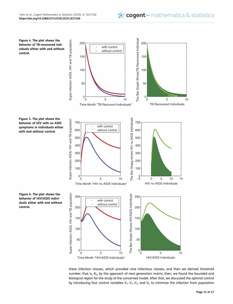
7. Numerical simulation and discussionIn this subsection of the article, the numerical simulations of the proposed model (1) are presented forverification of analytical results. The numerical results are obtained by using the Runge–Kutta methodof order 4. The parameter values used in the simulation are given in Table 1, which are biologicallyfeasible. Moreover, the time interval is taken from 0 to 10 units, while the different initial populationsize for the compartmental population is given in Figures 1–9 with and without vaccination and the bargraph of the related population is also obtained. By using the parameter values, non-negative initialpopulation sizes and the time interval 0 to 10 are shown in Table 1. From Figures 1–9, it is clear thatrecovery is fast in case of vaccination, while it is also to be noted that our proposed model shows thatthe TB/HIV and AIDS individuals show some different behaviors. Moreover, here we concluded thatvaccination provided for a long time will permanently eradicate the infection from the population. Hereour numerical results also show the area involved in the population or in the community.
Tahir et al., Cogent Mathematics & Statistics (2019), 6: 1637166https://doi.org/10.1080/25742558.2019.1637166
Page 11 of 17

8. Conclusion of the proposed modelIn this article, we extended the co-infection mathematical model for TB/HIV and chronic stage HIV(AIDS) defined in (Tahir & Shah, 0000). For this purpose, first we formulated the model according to
0 5 10−100
0
100
200
300
400
Time Month "Susceptible Individuals"
Sup
er in
fect
ion
AID
S, H
IV a
nd T
B p
opul
atio
n
with controlwithout contro l
0 5 10−100
0
100
200
300
400
Susceptible individuals
The
Bar
Gra
ph S
how
s su
scep
tible
Indi
vidu
alsFigure 1. The plot shows the
behavior of susceptible indivi-duals either with and withoutcontrol.
0 5 100
50
100
150
200
250
300
350
Time Month "Latent TB Individuals"
Sup
er in
fect
ion
AID
S, H
IV a
nd T
B p
opul
atio
n
with controlwithout control
0 5 100
50
100
150
200
250
300
350
Latent TB Individuals
The
Bar
Gra
ph s
how
sLat
ent T
B In
divi
dual
sFigure 2. The plot shows thebehavior of Latent TB indivi-duals either with and withoutcontrol.
0 5 100
50
100
150
200
250
300
350
Time Month "Latent TB Individuals"
Sup
er in
fect
ion
AID
S, H
IV a
nd T
B p
opul
atio
n
with controlwithout control
−5 0 5 10 150
50
100
150
200
250
300
350
The
Bar
Gra
phLa
tent
TB
Indi
vida
uls
Figure 3. The plot shows thebehavior of active TB indivi-duals either with and withoutcontrol.
Tahir et al., Cogent Mathematics & Statistics (2019), 6: 1637166https://doi.org/10.1080/25742558.2019.1637166
Page 12 of 17
there infection classes, which provided nine infectious classes, and then we derived thresholdnumber, that is, R0, by the approach of next-generation matrix; then, we found the bounded andbiological region for the study of the concerned model. After that, we discussed the optimal controlby introducing four control variables V1;V2;V3, and V4 to minimize the infection from population
0 5 100
50
100
150
200
Time Month "TB Recoverd Individuals"
Sup
er in
fect
ion
AID
S, H
IV a
nd T
B p
opul
atio
n
with controlwithout control
0 5 100
50
100
150
200
TB Recovered Individuals
The
Bar
Gra
ph S
how
sTB
Rec
over
ed In
divi
dualFigure 4. The plot shows the
behavior of TB-recovered indi-viduals either with and withoutcontrol.
0 5 100
100
200
300
400
500
600
700
Time Month "HIV no AIDS Individuals"
Sup
er in
fect
ion
AID
S, H
IV a
nd T
B p
opul
atio
n
with controlwithout control
−5 0 5 10 150
100
200
300
400
500
600
700
HIV no AIDS Individuals
The
Bar
Gra
pg s
how
s H
IV n
o A
IDS
Indi
vidu
alsFigure 5. The plot shows the
behavior of HIV with no AIDSsymptoms in individuals eitherwith and without control.
0 5 100
50
100
150
200
250
Time Month "HIV/AIDS Individuals"
Sup
er in
fect
ion
AID
S, H
IV a
nd T
B p
opul
atio
n
with controlwithout control
0 5 100
50
100
150
200
250
HIV/AIDS Individuals
The
Bar
Gra
ph S
how
s H
IV/A
IDS
Indi
vidu
alsFigure 6. The plot shows the
behavior of HIV/AIDS indivi-duals either with and withoutcontrol.
Tahir et al., Cogent Mathematics & Statistics (2019), 6: 1637166https://doi.org/10.1080/25742558.2019.1637166
Page 13 of 17

0 5 10−20
0
20
40
60
80
100
Time Month "Active TB/HIV infected Individuals"
Sup
er in
fect
ion
AID
S, H
IV a
nd T
B p
opul
atio
n
with controlwithout control
−5 0 5 10 15−20
0
20
40
60
80
100
Active TB/HIV Infected Individuals
Act
ive
TB
/HIV
Infe
cted
Indi
vidu
als
Figure 9. The plot shows thebehavior of active TB/HIV-infected individuals either withand without control.
0 5 100
20
40
60
80
100
Time Month "Latent TB/HIV infected Individuals"
Sup
er in
fect
ion
AID
S, H
IV a
nd T
B p
opul
atio
n
with controlwithout control
−5 0 5 10 150
20
40
60
80
100
Latent TB/HIV Infected Individuals
Late
nt T
B/H
IV In
fect
ed In
divi
dual
s
Figure 8. The plot shows thebehavior of latent TB/HIV-infected individuals either withand without control.
0 5 100
20
40
60
80
100
120
140
Time Month "HIV infected Individuals"
Sup
er in
fect
ion
AID
S, H
IV a
nd T
B p
opul
atio
n
with controlwithout control
−5 0 5 10 150
20
40
60
80
100
120
140
HIV Infected Individuals
The
Bar
Gra
ph S
how
s H
IV In
fect
ed In
divi
dual
sFigure 7. The plot shows thebehavior of HIV-infected indivi-duals either with and withoutcontrol.
Tahir et al., Cogent Mathematics & Statistics (2019), 6: 1637166https://doi.org/10.1080/25742558.2019.1637166
Page 14 of 17

and the behavior is shown in the graphs in Figure 1–9 with and without control. We observed thatwith vaccination, the recovery of individuals is very fast from the figures. All the parameters andtheir values are given in Table 1. Also, the simulation results are new in this area of research.
AcknowledgementsAll authors read and approved the final version.
FundingThe authors received no direct funding for this research.
Author detailsMuhammad Tahir1
E-mail: [email protected] ID: http://orcid.org/0000-0003-4300-3861Syed Inayat Ali Shah1
E-mail: [email protected] Zaman2
E-mail: [email protected] Department of Mathematics, Islamia College, Peshawar,KPK 25000, Pakistan.
2 Department of Mathematics, University of Malakand,Chakdara District Lower Dir, KPK, Pakistan.
Authors contributionAll authors equally contributed to this paper.
Conflict of InterestThere is no conflict of interest regarding this paper.
Citation informationCite this article as: Prevention strategy for superinfectionmathematical model tuberculosis and HIV associatedwith AIDS, Muhammad Tahir, Syed Inayat Ali Shah & GulZaman, Cogent Mathematics & Statistics (2019), 6:1637166.
ReferencesAbout HIV/AIDS. (2015, December 6) CDC.Basic Statistics. (2015, November 3). CDC.Cunningham, A. L., Donaghy, H., Harman, A. N., Kim, M., &
Turville, S. G. (2010). Manipulation of dendritic cell
Table 1. Description of parameter and its values
Notation Parameter description Value
μ The rate of recruitment 0:0235
dn Natural death rate 0:0213
γ1 Parameter of modification 0:1123
γ2 Parameter of modification 0:11889
k1 The rate through which individuals left LT ðtÞ class and got infection 0:0125
k2 The rate through which individuals left LTHðtÞ class and got TB infection 0:0825
k3 The rate through which individuals left LTHðtÞ class 0:2358
τ1 Rate for TB treatment in LT ðtÞ individuals 0:2230
τ2 Rate for TB treatment in IT ðtÞ individuals 0:2893
dT Death rate induced by TB 0:1110
δ Parameter of modification 0:3100
ρ1 The rate through which individuals left IHðtÞ class to A 0:5000
ρ2 The rate through which individuals left ITHðtÞ class 0:5800
ϕ The rate of HIV treatment in IHðtÞ individuals 0:1969
α1 The AIDS treatment rate 0:0035
α2 The rate of HIV treatment in AT ðtÞ individuals 1:0000
ω1 The rate through which individuals left CHðtÞ class 0:1030
ω2 The rate through which individuals left RHðtÞ class 0:0921
dA Death rate induced by AIDS 0:0035
r Fraction of LTHðtÞ treatment rate of HIV and TB individuals 0:6660
λ Individuals having active TB rate and susceptible 0:2345
λh Active HIV rate individuals 0:345
u1 Use a control parameter 0:2212
u1 Use a control parameter 0:0011
β1 The rate of TB transmission 1:7000
β2 The rate of HIV transmission 0:1000
dTA Death rate induced by AIDS-TB 0:2100
ηC Parameter of modification 0:0900
ηA Parameter of modification 0:6000
Tahir et al., Cogent Mathematics & Statistics (2019), 6: 1637166https://doi.org/10.1080/25742558.2019.1637166
Page 15 of 17

function by viruses. Current Opinion in Microbiology,13(4), 524–529. PMID 20598938. doi:10.1016/j.mib.2010.06.002.
Doitsh, G., Galloway, N. L. K., Geng, X., Yang, Z.,Monroe, K. M., Zepeda, O., … Greene, W. C. (2014). Celldeath by pyroptosis drives CD4 T-cell depletion inHIV-1 infection. Nature, 505(7484), 509–514. PMC4047036?Freely accessible. PMID 24356306.doi:10.1038/nature12940.
Evian, C. (2006). Primary HIV/AIDS care: A practical guidefor primary health care personnel in a clinical andsupportive setting. (4th ed, pp. 29). Houghton [SouthAfrica]: Jacana. ISBN 978-1-77009-198-6.
Fact sheet - Latest statistics on the status of the AIDSepidemic | UNAIDS. www.unaids.org 2017.
HIV/AIDS Fact sheet N360. WHO. November 2015Hu, D. (2001). Radiology of AIDS. Berlin [u.a.]: Springer. pp.
19. ISBN 978-3-540-66510-6.International Committee on Taxonomy of Viruses.
(2002a). 61.0.6. Lentivirus. National Institutes ofHealth.
International Committee on Taxonomy of Viruses.(2002b). 61. Retroviridae. National Institutes ofHealth.
Khan, M. A., et al. (2012). Optimal compaign in leptos-pirosis epidemic model by multiple control variables.Applied Mathematics, 3, 1655–1663. doi:10.4236/am.2012.311229
Khan, M. A., Zaman, G., Islam, S., & Chohan, M. I. (2013a).Application of homotopy perturbation method tovector host epidemic model with non-linearincidences. Research Journal of Recent Sciences, 2,90–95.
Khan, M. A., Islam, S., Ullah, M., Khan, S. A., Zaman, G.,Arif, M., & Sadiq, S. F. (2013b). Analytical solution ofthe leptospirosis epidemic model by homotopy per-turbation method. Research Journal of RecentSciences, 2, 66–71.
Kumar, V., Abbas, A. K., Fausto, N., & Mitchell, R. N. (2007).Robbins basic pathology (8th ed, pp. 516–522).Saunders Elsevier. ISBN 978-1-4160-2973-1.
Lawn, S. D., & Zumla, A. I. (2011, July 2). Tuberculosis.Lancet, 378(9785), 57–72. doi:10.1016/S0140-6736(10)62173-3.
Lenhart, S., & Workman, J. T. (2007). Optimal controlapplied to biological models, in: Mathematical andcomputational biology series. London, UK: Championand Hall, CRC.
Mandell, B., & Dolan (2010). Chapter 118.Markowitz, edited by William N. Rom; associate editor,
Steven B. (2007). Environmental and occupationalmedicine (4th ed.). Philadelphia: Wolters.
Sweilam, N. H., & Mekhlafi, S. M. A. L. “On the optimalcontrol for fractional multi-strain TB model” 10March 2016 doi:10.1002/oca.2247.
Tahir, M., Shah, S. I. A., Zaman, G., & Khan, T. (2018).Prevention strategies for mathematical modelMERS-corona virus with stability analysis and optimalcontrol. Journal of Nanoscience and Nanotechnology, 2,401.
Tahir, M., & Shah, S. I. A. (0000). A mathematicalco-infection problem its transmission and behaviouris presented with stability analysis. SeMA Journal.doi:10.1007/s40324-018-0176-y
Tahir, M., Shah, S. I. A., & Zaman, G. (2018). Approach foroptimal control to prevent infectious diseases fromcommunity. Journal of Advanced Physics, 7, 478–486.doi:10.1166/jap.2018.1467
Tuberculosis. (2002). World Health Organization.Tuberculosis Fact sheet N104. (2015, October). WHO.UNAIDS, WHO. (2007, December). 2007 AIDS epidemic
update (PDF). p. 10 doi:10.1094/PDIS-91-4-0467BWin Min, H., Apornpong, T., Kerr, S. J., Hiransuthikul, A.,
Gatechompol, S., Do, T., Ruxrungtham, K.,& Avihingsanon, A. (2018). CD4/CD8 ratio normalizationrates and low ratio as prognostic marker for non-AIDSdefining events among long-term virologically sup-pressed people living with HIV. AIDS Research andTherapy. doi:10.1186/s12981-018-0200-4
WHO. (2007). WHO case definitions of HIV for surveillanceand revised clinical staging and immunological clas-sification of HIV-related disease in adults and chil-dren. (PDF). Geneva: World Health Organization. pp.6–16. ISBN 978-92-4-159562-9.
Zaman, G., Kang, Y. H., & Jung, I. H. (2009). Optimaltreatment of an SIR epidemic model with time delay.Biosystems, 98, 43–50. doi:10.1016/j.biosystems.2009.05.006
Tahir et al., Cogent Mathematics & Statistics (2019), 6: 1637166https://doi.org/10.1080/25742558.2019.1637166
Page 16 of 17

© 2019 The Author(s). This open access article is distributed under a Creative Commons Attribution (CC-BY) 4.0license..
You are free to:Share — copy and redistribute the material in any medium or format.Adapt — remix, transform, and build upon the material for any purpose, even commercially.The licensor cannot revoke these freedoms as long as you follow the license terms.
Under the following terms:Attribution — You must give appropriate credit, provide a link to the license, and indicate if changes were made.You may do so in any reasonable manner, but not in any way that suggests the licensor endorses you or your use.No additional restrictions
Youmay not apply legal terms or technological measures that legally restrict others from doing anything the license permits.
Cogent Mathematics & Statistics (ISSN: 2574-2558) is published by Cogent OA, part of Taylor & Francis Group.
Publishing with Cogent OA ensures:
• Immediate, universal access to your article on publication
• High visibility and discoverability via the Cogent OA website as well as Taylor & Francis Online
• Download and citation statistics for your article
• Rapid online publication
• Input from, and dialog with, expert editors and editorial boards
• Retention of full copyright of your article
• Guaranteed legacy preservation of your article
• Discounts and waivers for authors in developing regions
Submit your manuscript to a Cogent OA journal at www.CogentOA.com
Tahir et al., Cogent Mathematics & Statistics (2019), 6: 1637166https://doi.org/10.1080/25742558.2019.1637166
Page 17 of 17