Tutorial

Version 1.0 September 2014

Project Team

Theresa Nelson

Aaron Ruesch

Danica Mazurek

Sarah Kempen

David Evans

dnrwaterqualitymodeling@wisconsin.gov

i

DISCLAIMER

EVAAL, the included documentation, and sample data files are made available free on an "as is"

basis. Although the Wisconsin Department of Natural Resources (WDNR) has tested this

program, no warranty, expressed or implied, is made by WDNR as to the accuracy and

functioning of the program and related program material. Neither shall the fact of distribution

constitute any such warranty nor is responsibility assumed by WDNR in connection therewith.

The contents of this manual are not to be used for advertising, publication, or promotional

purposes.

This tutorial assumes that the user has a moderate to intermediate knowledge of ArcGIS

software, GIS processing, and GIS datasets.

ii

TABLE OF CONTENTS

1.0 OVERVIEW ................................................................................................................. 1

2.0 HOW DOES EVAAL WORK? .................................................................................... 1

3.0 SYSTEM REQUIREMENTS ....................................................................................... 2

4.0 EVAAL INPUTS .......................................................................................................... 2

5.0 EVAAL SETUP ............................................................................................................ 4

5.1 Accessing and setting up EVAAL files.................................................................4

5.2 Loading EVAAL ...................................................................................................5

6.0 RUNNING EVAAL...................................................................................................... 6

6.1 Step 1: Condition the LiDAR DEM ......................................................................7

6.2 Identify Internally Drained Areas .........................................................................7

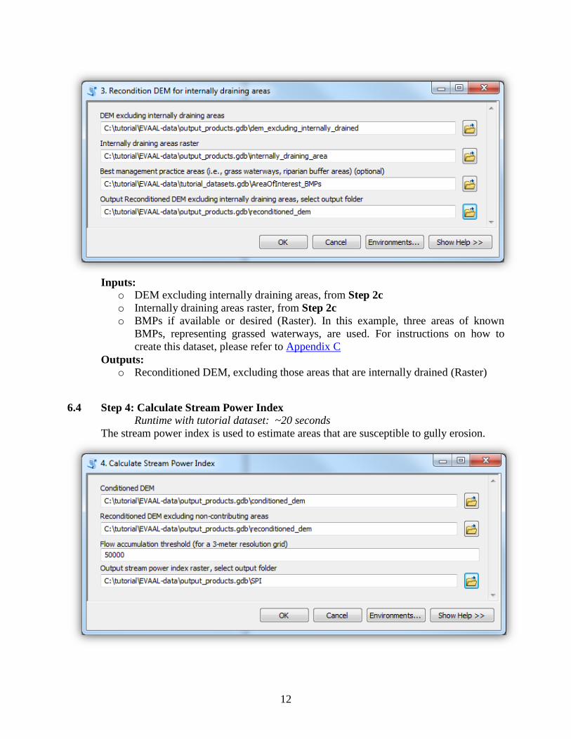
6.3 Step 3: Recondition DEM for internally draining areas ......................................11

6.4 Step 4: Calculate Stream Power Index ................................................................12

6.5 Step 5: Estimating Sheet and Rill Erosion ..........................................................13

6.6 Step 6. Calculate Erosion Vulnerability Index ....................................................17

7.0 OUTPUT OPTIONS ................................................................................................... 19

7.1 Modifying the Frequency-Duration of Precipitation Input .................................19

7.2 Creating Different Management Scenarios .........................................................19

8.0 TROUBLESHOOTING .............................................................................................. 19

9.0 TECHNICAL SUPPORT ........................................................................................... 21

10.0 APPENDICES .......................................................................................................... 22

Appendix A Creating Culverts Layer ........................................................................22

Appendix B Data Acquisition ...................................................................................24

Appendix C ArcGIS Tasks .......................................................................................25

Appendix D Output Files ..........................................................................................28

iii

ACRONYMS

BMP: Best Management Practice

CDL: Cropland Data Layer

CLU: Common Land Unit

DEM: Digital Elevation Model

EVAAL: Erosion Vulnerability Assessment for Agricultural Lands

GIS: Geographic Information System

gSSURGO: gridded Soil Survey Geographic Database

HUC: Hydrologic Unit Code

LiDAR: Light Detection And Ranging

NASS: National Agricultural Statistics Service

NRCS: Natural Resource Conservation Service

SPI: Stream Power Index

TMDL: Total Maximum Daily Load

USDA: United States Department of Agriculture

USLE: Universal Soil Loss Equation

WDNR: Wisconsin Department of Natural Resources

1

1.0 OVERVIEW

The Wisconsin Department of Natural Resources (WDNR) Bureau of Water Quality has

developed EVAAL, the Erosion Vulnerability Assessment for Agricultural Lands, to assist

watershed managers in prioritizing areas within a watershed which may be vulnerable to water

erosion (and associated nutrient export) and which may contribute to downstream water quality

problems. It evaluates locations of relative vulnerability to sheet, rill, and gully erosion using

information about topography, soils, rainfall, and land cover. This tool is intended for relatively

small watersheds (less than ~75 km2) that have already been identified as watersheds that

contribute higher nonpoint source pollutant loads, such as subbasins identified in a Total

Maximum Daily Load (TMDL) study as relatively high-loading. This tool enables watershed

managers to prioritize and focus their field-scale data collection efforts, thus saving time and

money while increasing the probability of locating fields with high sediment and nutrient export

for implementation of BMPs.

This tutorial demonstrates the application of EVAAL on a subbasin of the Plum Creek watershed

in eastern Wisconsin. It is approximately 5.5 km2 in area with land use dominated by agricultural

activity. Tutorial data is available for download from the WDNR ftp site

(ftp://dnrftp01.wi.gov/geodata/EVAAL_V1_0) as two Esri file geodatabases, one that provides

the input data needed to successfully run EVAAL, and another containing EVAAL outputs for

the watershed. Only the data in the input geodatabase is needed to run EVAAL; the data in

output geodatabase is provided for comparison to the user’s own output. Note that individual tool

runs may not provide the exact same results, as difference in areas included and parameters

chosen will likely influence the result.

Detailed information regarding the methods applied in this tutorial can be found in the

companion document, EVAAL Methods Documentation. That report contains an introduction to

the tool development, descriptions of the model inputs, the methodologies applied, and the model

outputs, as well as a comparison to another commonly used soil loss model, example

applications of the model, references, and appendices.

2.0 HOW DOES EVAAL WORK?

The EVAAL toolset was designed to quickly identify areas vulnerable to erosion using readily

available data and a user-friendly interface. This tool estimates vulnerability by separately

assessing the risk for sheet and rill erosion (using the Universal Soil Loss Equation, USLE), and

gully erosion (using the Stream Power index, SPI), while deprioritizing those areas that are not

often hydrologically connected to surface waters (also known as internally drained, or non-

contributing areas). These three pieces are combined to produce the following outputs:

erosion vulnerability index for the area of interest (raster and tabular);

areas vulnerable to sheet and rill erosion;

areas of potential gully erosion;

areas hydrologically disconnected from surface waters.

2

It is important to note that erosion “vulnerability” refers to an area’s susceptibility to sediment

and nutrient runoff given certain, assumed management practices. The erosion vulnerability

index output is a relative, non-dimensional index, which means that output from separate model

runs should not be compared directly. Direct comparison is only advisable for areas that have

been included in the same model run. The erosion vulnerability output is a non-dimensional

index, meaning it is only intended to prioritize or rank, not estimate the real value of sediment or

nutrient runoff.

EVAAL is an ArcGIS Toolbox divided into several different tools, to facilitate greater control

over inputs. The workflow can be divided into several stages: creating a hydrologically

conditioned DEM, identifying and removing from analysis those areas on the landscape that do

not drain to surface waters, estimation of potential gully erosion, estimation of relative soil loss

potential from sheet and rill erosion, and the calculation of an erosion vulnerability index.

For more information on the methods underlying the tools and processes, users are encouraged to

read the Methods Documentation for EVAAL.

3.0 SYSTEM REQUIREMENTS

To successfully install and operate EVAAL, the following requirements are needed:

Minimum 1.50 GB of RAM

ESRI ArcGIS 10.1 or 10.2 Desktop

ESRI ArcGIS 10.1 to 10.2 Spatial Analyst Extension

The tool makes use of several functions in ArcGIS’s Spatial Analyst Extension and so it

is necessary to have access to this license. To verify it is available select the ArcMap

Toolbar, move down to Customize, select Extensions, and check the “Spatial Analyst”

box. If you do not have access to the Spatial Analyst extension, contact your system

administrator for information on how to gain access.

4.0 EVAAL INPUTS

EVAAL has several input data files that are required in order to run. It is recommended that

these files be formatted within an ESRI file geodatabase, but is not required. Refer to Appendix

B for instructions on how to obtain the required datasets for areas outside the tutorial dataset

domain. All input data must be in the Wisconsin Transverse Mercator geographic

projection (EPSG: 3071) (ftp://dnrftp01.wi.gov/geodata/projection_file/).

LiDAR DEM

High quality, fine scale elevation data (less than 3-meter X/Y resolution) is

central to this tool and to the accurate modeling of landscape scale hydrology.

LiDAR data is available for numerous Wisconsin counties, some of which are

freely available on the WisconsinView website (http://wisconsinview.org/)

3

Area of Interest/Watershed Boundary

This is used to define the area in which erosion vulnerability is to be assessed. It

is strongly recommended to be a watershed boundary less than 75 square

kilometers. The tool may or may not run to completion on areas larger than

recommended. Certain functions of EVAAL require a buffered version of the area

of interest; instructions for creating a buffered version of the area of interest can

be found in Appendix C.

gSSURGO Data

EVAAL requires information about the erodibility of local soils. The tool was

written specifically to access this data from the statewide Gridded Soil Survey

Geographic Database, or gSSURGO database. The gSSURGO database is freely

available from the USDA-NRCS Geospatial Datagateway. Note that this is a

statewide dataset and so is very large and can take several hours to download.

Culvert Polylines

The LiDAR DEMs are of such high resolution that features such as road berms

are clearly discernable and create what are known as “digital dams”. When

hydrologic terrain attributes are calculated, these digital dams make it seem as

though the flow of water is being impeded as it runs over the landscape. In order

to accurately determine if rain water is likely to run off into surface waters or if it

will pond and infiltrate before reaching surface waters, it is necessary to “break”

these dams. This requires a vector layer of culverts to be created for the area of

interest. See Appendix A for instructions on how to create the culverts layer; note

that this must be done prior to running the tools.

EVAAL also uses the following data, but the user is not required to download or provide it prior

to running the tool, provided an internet connection is available; the capability to automatically

download and process this data is built into the tool.

Frequency-Duration Precipitation Data

Precipitation amounts for a given frequency and duration of storm event is

available from the National Weather Service. This information is used to assess if

an area on the landscape is hydrologically connected to surface waters, given a

specified size storm event.

National Cropland Data Layer (CDL)

Data about specific crops grown in an area are produced from the National

Agricultural Statistics Service (NASS). These data layers are used to infer a

generalized agricultural management scheme from a crop rotation sequence. For

example, 2 years of corn, 1 year of soybeans, and 2 years of alfalfa would be

considered a dairy rotation. It is recommended to use at least 5 years of data to

determine the generalized rotations. For more information on how a generalized

crop rotation is created, users should consult the EVAAL methods documentation.

4

Within the tool are the options to use additional datasets to customize the output.

Zone boundaries

These are vector files that delineate specific zones within the area of interest and

are used to aggregate the erosion vulnerability index or other output values. For

example, these boundaries could be for tracts, agricultural fields, or tax parcels.

The default of EVAAL is to calculate erosion vulnerability for every grid cell on

the landscape. In order to assess which agricultural fields or tracts have the most

potential for erosion, the zone boundary input layer can be used to average the

erosion vulnerability index for each field or tract.

Best Management Practices (BMPs)

A raster layer of digitized BMP locations can be used to deprioritize areas that

already have BMPs currently installed. Examples of these features are grassed

waterways, strip cropping, cover crops, and riparian buffers, see Appendix C for

assistance in creating this file.

5.0 EVAAL SETUP

5.1 Accessing and setting up EVAAL files

The most recent version of EVAAL can be downloaded from the DNR Water Quality

Modeling team’s GitHub repository, under the project name of “EVAAL”

(https://github.com/dnrwaterqualitymodeling/EVAAL). Once at this page select the

button on the right-hand side of the page labeled “Download ZIP”.

The tools and associated files are downloaded as one zip file. The file should be unzipped

to a directory to which all users must have permission to write. In addition, there may not

5

be spaces or “reserved”1 characters within the folder pathname. For this tutorial, the

model files were unzipped to a folder called “tutorial.” The input datasets are available

for download from ftp://dnrftp01.wi.gov/geodata/EVAAL_V1_0. The geodatabase

containing the tutorial inputs is titled “tutorial_datasets.gdb.” It is recommended that the

user create a geodatabase to hold the outputs of EVAAL, this has been done for the

tutorial and is called “output_products.gdb” in this example. Instructions on how to create

a geodatabase are located in Appendix C.

5.2 Loading EVAAL

EVAAL was designed to be used with ArcGIS 10.1 or 10.2. It can be run from ArcMap

or from ArcCatalog. Running from the latter will limit any issues with schema locks,

though this tutorial demonstrates running the tools from ArcMap in order to show images

of the output files as they are created. EVAAL runs as a series of scripts in a Python

Toolbox, this allows for an easy interface from within ArcGIS. To access and run the

scripts from ArcMap, open the ArcToolbox window, right-click within this window and

select “Add Toolbox…”, then navigate to where the file from GitHub was unzipped,

open the “EVAAL-master” folder, and select the “__EVAAL__.pyt” toolbox.

1 “Reserved” characters include: ?, %, *, :, “, |, <, >, and “.”.

Code and documents downloaded from GitHub

Output geodatabase and tables

Input files necessary for program

6

This toolbox should now show up in the ArcToolbox window. Upon opening this

toolbox, ten functions should be visible. To ensure the tool is visible every time the user

opens ArcMap or ArcCatalog, right-click the ArcToolbox again, then “Save Settings”,

then click “To Default.”

A note on terminology: this program is implemented as an ArcGIS Toolbox, and so each

individual step is, in ArcGIS terminology, a tool. For our purposes, these ten steps will be

referred to as steps or functions, to avoid confusion between the EVAAL toolset,

ArcToolboxes, and tools.

6.0 RUNNING EVAAL

To conceptualize the workflow for EVAAL, it is helpful to group the functions within the

EVAAL toolset, therefore these functions have been given numbers and letters to group them

according to their purpose. Note that if the user is running the functions from ArcMap 10.1 the

output files WILL NOT be automatically added to your map document (this is an unfortunate

ArcGIS bug). As a result, if the user would like to view the files created from any step, the user

needs to “Add Data…” and open the output files in their ArcMap document. Additionally, users

should remember to always specify the output folder for the output files, to avoid confusion and

misplaced files. Runtimes given are for the tutorial dataset, a watershed approximately 5.5 square

kilometers (2.5 square miles) in area, on a computer with a 64-bit Intel Xeon processor and 6 GB

of RAM; running the analyses on larger watersheds or “slower” computers will result in longer

runtimes. For the tutorial area of interest, output files are included in the “output_products.gdb”

and images of these files are found in Appendix D. If errors are encountered, users are

encouraged to consult the Troubleshooting section of this tutorial.

7

6.1 Step 1: Condition the LiDAR DEM

Runtime with tutorial dataset: ~8 minutes

This step utilizes the culverts layer that has already been created. Note that for large areas

of interest this step will have a long runtime (e.g., for areas nearing 50 square kilometers,

expect several hours).

Inputs:

o Culverts – feature class to break digital dams (Polyline feature class)

o Watershed boundary – or boundary for area of interest (Polygon feature class)

o Raw LiDAR DEM – DEM (needs to be larger than area of interest) from which

the watershed of interest is being cut (Raster)

Outputs:

o Conditioned DEM – the DEM modified for more accurate drainage assessment

(Raster)

o Optimized fill – a DEM which has been modified so all the water drains off the

landscape (Raster)

6.2 Identify Internally Drained Areas

These steps assess if an area on the landscape will store water or if the water will run off

into a stream or lake. Areas which do not drain to surface waters (i.e., drain internally)

are deprioritized in this analysis as they are considered to be hydrologically disconnected

from surface waters and therefore do not directly contribute to surface water quality

issues.

8

6.2.1 Step 2a: Download Precipitation Data

Runtime with tutorial dataset: ~ 30 seconds

The frequency-duration precipitation data is used to assess which areas will drain to

surface waters and which areas will not, given a user-defined rainfall event. The larger

the storm (the less frequent and the longer duration) selected, the fewer areas that will be

considered as disconnected to surface waters and not contributing to runoff.

Inputs:

o Desired frequency and duration to use in analysis (a 10-yr, 24-hr storm is

recommended, but the user can change as desired)

OR

o Zip file of locally stored precipitation data (use check box at top to toggle this

option). For instructions on how to acquire this data, see Appendix B.

o Conditioned DEM from Step 1 for use as a template

Outputs:

o The frequency-duration precipitation layer (Raster)

6.2.2 Step 2b: Create Curve Number Raster

Runtime with tutorial dataset: ~ 3 minutes

The curve number method is a way of estimating the amount of runoff. This estimate

considers land use, land cover and the hydrologic soil group, which is based on

infiltration rate. It also depends on factors such as type and amount of tillage, and amount

of year-round residue/crop cover. Such factors are difficult to assess without direct

observation, and so the function outputs both a high estimate of the runoff potential (high

curve number) and a low estimate of runoff potential (low curve number). It is left to the

user to decide whether to assume that management in their area of interest is generally

9

facilitating infiltration (low curve number) or if management is hindering infiltration

(high curve number).

Inputs:

o Starting and ending years for cropland layers to download (recommended to use

at least five years)

OR

o Location of local cropland layers (use check box at top to toggle this option)

o Location of gSSURGO database, select just the geodatabase file, not specific

tables or files within. For instructions on how to acquire this data, see Appendix

B.

o Buffered watershed boundary (Polygon Feature Class)

10

o Conditioned DEM from Step 1 for use as a template

Outputs:

o Output curve number raster, high estimate (Raster)

Assuming management practices that increase runoff

o Output curve number raster, low estimate (Raster)

Assuming management practices that reduce runoff

6.2.3 Step 2c. Identify internally draining areas

Runtime using tutorial dataset: ~3 minutes

This function utilizes the output from the previous steps to identify those areas that are

disconnected to surface waters and do not contribute to runoff, given a certain storm

event. Note that this tool must be run twice if the user wants to use both curve number

estimates in later steps. If no internally draining areas are found in the area of interest,

this function will return a message saying so. It will produce a file for the internally

draining areas and a DEM excluding internally draining areas, but the former will be null

and blank and the latter will be identical to the conditioned DEM. Because the following

step expects these output files, input them in Step 3, as if there were internally drained

areas.

11

Inputs:

o Conditioned DEM, from Step 1

o Optimized fill raster, from Step 1

o Precipitation frequency-duration, from Step 2a

o Curve number raster (either high or low; in this example practices that increase

runoff are assumed and the high curve number is used), from Step 2b

o Buffered watershed boundary (Polygon Feature Class)

Outputs:

o Internally draining areas, shows those areas of the landscape found not to be

connected to surface waters (Raster)

o DEM excluding internally draining areas, a modified DEM with non-contributing

areas removed (Raster)

6.3 Step 3: Recondition DEM for internally draining areas

Runtime with tutorial dataset: ~30 seconds

This step produces a reconditioned DEM that accounts for areas that do not contribute to

runoff. This is similar to what was produced in Step 1, but it now has the non-

contributing areas removed from the DEM.

12

Inputs:

o DEM excluding internally draining areas, from Step 2c

o Internally draining areas raster, from Step 2c

o BMPs if available or desired (Raster). In this example, three areas of known

BMPs, representing grassed waterways, are used. For instructions on how to

create this dataset, please refer to Appendix C

Outputs:

o Reconditioned DEM, excluding those areas that are internally drained (Raster)

6.4 Step 4: Calculate Stream Power Index

Runtime with tutorial dataset: ~20 seconds

The stream power index is used to estimate areas that are susceptible to gully erosion.

13

Inputs:

o Conditioned DEM, from Step 1

o Reconditioned DEM, excluding non-contributing areas, from Step 3

o Flow Accumulation Threshold, the default value of 50000 is recommended,

though the capability is provided for advanced users interested in altering the flow

accumulation threshold. Raising this value will include longer flow paths,

potentially modeling streamflow as opposed to overland flow. Alternatively,

lowering this value will shorten flow paths.

Outputs:

o Stream power index (Raster)

6.5 Step 5: Estimating Sheet and Rill Erosion

The Universal Soil Loss Equation (USLE) is used to estimate soil loss potential from

sheet and rill erosion. The version of the USLE in this tool calculates an index of soil loss

using rainfall erosivity, soil erodibility, slope/slope-length, and a land cover factor (see

Methodology document for additional details). The results of the USLE analysis should

be used relatively instead of quantitatively.

6.5.1 Step 5a: Rasterize K-factor for USLE

Runtime with tutorial dataset: ~2 minutes

The K factor is easily estimated for the area of interest by referencing the gSSURGO

database.

Inputs:

o Location of gSSURGO database, as in Step 2b, select just the geodatabase file,

not specific tables or files within

o K factor field, leave this as ‘kwfact’, unless you know that the title of this field in

the gSSURGO table has been modified

14

o Conditioned DEM, from Step 1

o Buffered watershed boundary (Polygon Feature Class)

Outputs:

o K factor showing the erodibility of the soils in the area of interest (Raster). Note

that there are a few locations in Wisconsin where soils were not surveyed—the

toolbox does not attempt to evaluate erosion vulnerability in these areas.

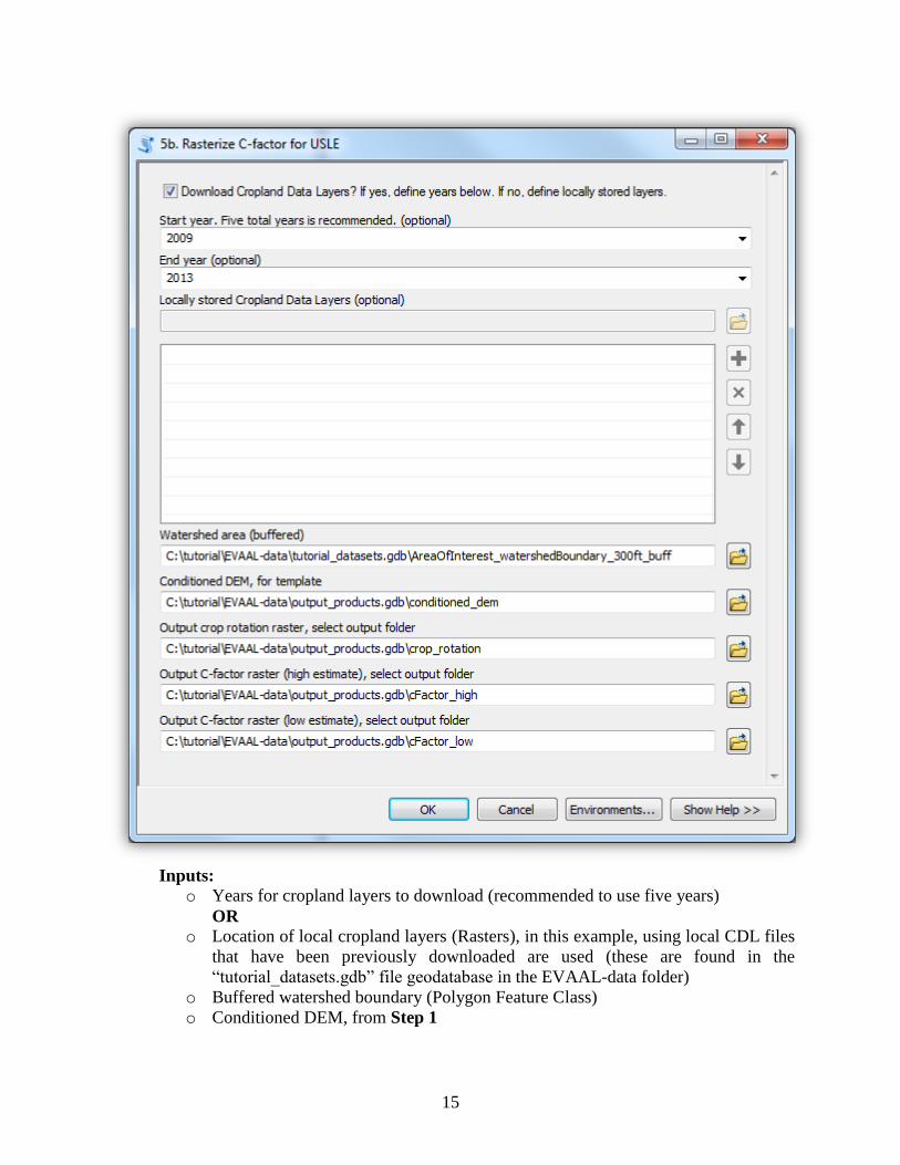
6.5.2 Step 5b. Rasterize C-factor for USLE

Runtime with tutorial dataset: ~1 minute

The Cropland Data Layer (CDL) is used to estimate the C factor by calculating a

probable crop rotation scenario. As there are potentially many variations in tillage and

cropping, the specifics of management cannot be estimated without direct observation.

As with the curve number, high and low C factors are calculated assuming management

practices that might enhance runoff and management practices that might reduce runoff,

respectively.

15

Inputs:

o Years for cropland layers to download (recommended to use five years)

OR

o Location of local cropland layers (Rasters), in this example, using local CDL files

that have been previously downloaded are used (these are found in the

“tutorial_datasets.gdb” file geodatabase in the EVAAL-data folder)

o Buffered watershed boundary (Polygon Feature Class)

o Conditioned DEM, from Step 1

16

Outputs:

o Crop rotation (Raster) map showing the estimated crop rotation, created from

cropland data layers (rotation descriptions are included in attribute table; to

symbolize this layer see Appendix C)

o C factor, high estimate, assuming practices contributing to erosion (Raster)

o C factor, low estimate, assuming conservation practices (Raster)

6.5.3 Step 5c. Calculate soil loss using USLE

Runtime with tutorial dataset: ~20 sec

When running the USLE, it is possible to define the rainfall erosivity factor. Erosivity is

generally understood to vary at coarse spatial scales, and so by default is assumed not to

vary in the study area. However, if it is known to vary within the watershed, the option is

available to input an erosivity raster or a user-specified constant. Note that to calculate

the soil loss with both the high C and low C factor estimates, it is necessary to run this

tool twice.

Inputs:

o Conditioned DEM, from Step 1

o Reconditioned DEM, from Step 3

o Optional erosivity values

A raster map of rainfall erosivity

OR

An erosivity constant

17

o K-factor, from Step 5a

o C-factor, from Step 5b, either high or low. In this example management is

assumed to be contributing to or at least not mitigating erosion, and so a high C

factor is used.

o Flow Accumulation Threshold, the default value of 1000 is recommended, though

the capability is provided for advanced users interested in altering the flow

accumulation threshold. As in Step 6.4, raising this value will include longer flow

paths, potentially modeling gully or even stream erosion as opposed to overland

sheet and rill erosion. Alternatively, lowering this value will shorten flow paths.

Outputs:

o Soil loss index map (Raster)

6.6 Step 6. Calculate Erosion Vulnerability Index

Runtime with tutorial dataset: ~20 seconds

The final step is to combine the susceptibility to gully erosion with the susceptibility to

sheet and rill erosion to produce the erosion index.

Inputs:

o Soil loss index raster, from Step 5c

o Stream power index, from Step 4

o Optional zonal boundary layer (Polygon Feature Class), such as CLU, tract, field

or tax parcel layers. This boundary layer is used to create a summary table of the

erosion index, with each record being a feature within the boundary layer. This

18

example uses a parcel boundary layer for the area, which contains fake data on the

tax parcels of the properties.

o Optional zonal statistic field which is the column name, by which the erosion

index should be summarized, defaults to each individual polygon in the layer.

This example summarizes the erosion index for each parcel within the area of

interest therefore “Parcel_ID” (the name of the column within the layer) is

entered.

o Conditioned DEM, from Step 1

Outputs:

o The erosion index map (Raster), this map shows the locations that are most

susceptible to sheet, rill, and gully erosion. Note that this is an optional output. If

the user is interested only in producing a tabular output do not enter a name here

and no file will be produced.

o Table showing summary statistics of the erosion vulnerability index, grouped by

the input boundaries. This allows for identifying those fields or landowners that

are potentially the most susceptible to erosion. (See Appendix C for displaying

this in a map.)

19

7.0 OUTPUT OPTIONS

EVAAL allows for different purposes and scenarios to be produced and explored.

7.1 Modifying the Frequency-Duration of Precipitation Input

The frequency-duration precipitation data is used to assess locations that drain to surface

waters and locations that do not have outflows and drain water internally. By increasing

the frequency and duration of the storm input, for example from the default 10-year 24-

hour storm to 100- or 500-year storm, the amount of area that drains internally decreases

as the simulated runoff overflows more of the depressions. A stronger storm creates

fewer internally drained areas, increasing the area included in calculating the erosion

index.

7.2 Creating Different Management Scenarios

The curve number is an estimate of the runoff potential for a certain soil given a certain

land cover. It is based on the hydrologic soil group as well as management factors such as

cover type and tillage. Similarly, the C factor in the USLE is derived from the amount of

canopy, surface cover, surface roughness, and prior land use. Both the C factor and curve

number need field-specific information to know how management factors impact their

values. For each of these, best- and-worst case scenarios are assumed, creating high and

low curve number and C factor output raster layers. It is left to the user whether the soil

erosion vulnerability index should be a worst- or best-case scenario. Or the user can run

the index twice, once for best-case and once for worst-case, then look at the difference

between the two outcomes; those areas with the greatest difference show areas where

there would be the greatest erosion reduction if going from poor to good management

practices.

8.0 TROUBLESHOOTING

EVAAL has been run, checked, and tested to catch and fix any potential errors in the underlying

code. There are still errors that can happen and below is a list of common and potential problems

and solutions.

Possible Issue 1: File open in another program

Message “WindowError: [Error 32] The process cannot access the file because it is

being used by another process: <filename>”

Problem The script cannot delete a file in the scratch geodatabase. This could be

because the scratch database is open or because of another issue with

ArcMap or ArcCatalog.

Possible

Solution Close ArcMap and/or ArcCatalog and try running the program again.

20

Possible Issue 2: Too many characters in name

Message “Could not save raster dataset to <filepath> with output format GRID” or

“Name of single band grid cannot have more than 13 characters”

Problem ArcGIS cannot save the file as a GRID format to a normal folder if the file

has too many characters in the name.

Possible

Solution

Save the file to a file geodatabase or if you would like to output the file to a

location outside a geodatabase, reduce the number of characters or save the

file as a TIFF (with a .tif extension).

Possible Issue 3: ArcCatalog won’t open at all or won’t open the EVAAL Toolset

folder and crashes

Message A window will open with the heading “ArcGIS Desktop has encountered a

serious application error and is unable to continue”

Problem There is a bug with the Python toolbox on which EVAAL runs.

Possible

Solution

The best solution seems to be to delete a results file that ArcGIS

automatically creates. Navigate to

C:\Users\<user>\AppData\Roaming\ESRI\Desktop10.x\ArcToolbox (where

you replace the <user> with your local username) and then delete the

“ArcToolbox.dat” file. Note that the AppData folder is a hidden folder, and

to find it is necessary to make all hidden folders visible or to type the above

path directly into Windows Explorer.

Possible Issue 4: Compact cannot execute

Message “ExecuteError: Failed to execute. Parameters are not valid. Error 000188:

Only supported by personal geodatabases

Failed to execute (Compact)”

Problem Issue with deleting or cleaning the scratch geodatabase.

Possible

Solution

Go into the EVAAL folder, and then into the ‘Scratch’ folder and delete

scratch.gdb

Possible Issue 5: There are lines of NoData on the Erosion Vulnerability Index output

Message No error message because the tool runs to completion

Problem There are some areas of the zonal statistics boundary layer that do not have

data and so the NoData values get transferred to the output.

Possible

Solution Rerun the tool without any zonal statistics layer.

Possible Issue 6: Where is the output?

Message No error message because the tool runs to completion

Problem The output maps are not automatically added to the map document or the

output file is not in the expected folder.

Possible

Solution

1. Add the the output manually to the map document

2. If you cannot find the output, check to make sure that you specified the

file path to your output geodatabase. Its possible the file is in your scratch

geodatabase within the scratch folder of the EVAAL folder or maybe your

default geodatabase.

21

Possible Issue 7: Error in reading/writing data

Message “ExecuteError: ERROR 999999: Error executing function. Workspace or

data source is read only.”

Problem Some functions run multiple procedures and cannot access local files.

Possible

Solution

1. Delete the scratch geodatabase in the “Scratch” folder within the EVAAL

code folder and restart the session.

2. Use ArcCatalog to avoid schema lock issues.

3. If error persits, see Issue 3, and delete the ArcToolbox.dat file.

9.0 TECHNICAL SUPPORT

Technical issues can be sent to dnrwaterqualitymodeling@wisconsin.gov and will be responded

to by one of the Wisconsin Department of Natural Resources Modeling Technical Team staff.

Updated versions of EVAAL, user’s manual, and documentation can be retrieved from the DNR

Water Quality Modeling Team’s GitHub.

Links to the model files, documentation, and tutorial data can be found on the WDNRs website:

http://dnr.wi.gov/topic/Nonpoint/EVAAL.html.

22

10.0 APPENDICES

Appendix A Creating Culverts Layer

The high resolution of the LiDAR DEM shows roads and highways in high relief. When

modeling water flow over the landscape, this creates “digital dams” that artificially impound the

water. In reality there are usually culverts or bridges that are allowing water to flow through road

berms and other barriers. To rectify this, it is necessary to create a layer of ‘culverts’ so that

water can flow unimpeded. To create this layer, follow these steps:

1. Create a “filled” DEM using the Fill tool in ArcGIS Spatial Analyst “Hydrology”

toolbox. This creates a map where all internally draining areas have been ‘filled up’

(elevation increased) so that all the water flows off of the map. Then subtract the

original DEM from the filled raster using the Spatial Analyst ‘Map Algebra’ “Raster

Calculator” (Fill – Dem). This results in a raster of the depression depths,

highlighting those areas that are not draining directly to streams.

2. Deep depressions near road berms are places where a culvert is probably located.

Locate one of these depressions using the depression depth raster, just created, and

zoom to it.

3. To visualize digital dams, open the “Symbology” tab in the original DEM’s

“Property” tab (found by right-clicking the layer in the table of contents). Choose the

Filled DEM Raw DEM

DEM

Depression Depth

23

“Stretched” option using “From Current Display Extent” with the Statistics box, and

choose a color gradient that spans multiple hues (e.g., a rainbow color scheme).

4. Create an empty line feature class. To do this, open the ArcCatalog window, and

right-click a geodatabase in which you would like the culverts layer. Select ‘New’

and select ‘Feature Class.’ Type the name of the culverts layer, and make sure to

select the “Line” type of feature. You may be prompted to select the coordinate

reference system for this layer, you can navigate to the

“NAD_1983_HARN_Transverse_Mercator” projection or you can copy and paste

this into the search bar and select this projection under the “Layers” tab. Select the

defaults for the remainder of the pages.

5. Start an editing session with this new feature. Right-click the new feature, and select

“Edit Features” and select “Start Editing.” The “Create Features” panel should open

on the side of ArcMap. If it does not, move to the editor tool bar and select the pencil

over the pad icon. Select the name of the layer that you have just created, and make

sure that the ‘Line’ function is highlighted in the “Construction Tools” window.

6. Each culvert should have only two nodes. The nodes must be drawn in order from

upstream to downstream, across the digital dam. Use the depression depth raster

created in Step 1 to navigate to impounded areas. Then switch to the original DEM to

identify the side of higher elevation and lay down the first node of the culvert. Then

click to lay down the downstream end of the culvert. After these two clicks, right

click and select “Finish Sketch” or just push F2 on your keyboard. It can be difficult

to be certain which locations are actually higher in elevation than those in the

downstream area, so it can be very helpful to use the “Identify” tool on the toolbar (

) to extract pixel elevations. While editing, save often by selecting the “Editor” on the

Editor Toolbar and select “Save Edits.”

24

7. Repeat this process until all digital dams have culverts spanning them. Then select the

“Editor” on the Editor Toolbar and select “Save Edits” and then “Stop Editing.” The

culverts layer has been completed.

Appendix B Data Acquisition

Refer to the following steps if you require any of the input data.

B1 LiDAR DEMs

To find LiDAR DEMs go the WisconsinView website. Here, LiDAR DEMs are available

in county wide downloads for certain counties. They are large files and so may take some

time to download. It is not necessary to clip the LiDAR DEM to the area of interest; the

script will do this automatically.

B2 gSSURGO Database

The gridded Soil Survey Geographic Database can be found on the USDA - NRCS

Geospatial Data Gateway website. On the menu on the right-hand side, select “Order by

State” and then select Wisconsin. Scroll down to the “Soils” section and check the box

next to “Gridded Soil Survey Geographic (gSSURGO) by State” box. Then select the

green “Continue” button at the bottom of the screen. Select continue again, and then enter

your contact information and the email you wish the download notification to be sent.

After this page, verify the info is correct and select “Place Order”. Within several minutes

you will receive an email message with a link to an FTP download. Click this and the

gSSURGO dataset will begin downloading (this is a large file and so may take some

time). Once it is done, unzip it to a folder of your choice – you may want to put it in the

same folder as your other input datasets. You need only navigate here to find the

geodatabase that the EVAAL function requires to complete its analysis.

B3 Cropland Data Layers

25

The CDL can be automatically downloaded by EVAAL. If you would like to see these

files for a larger area, you can find them at the USDA - NRCS Geospatial Data Gateway

website (where the gSSURGO database was found). At the homepage, you will need to

select the area in which you are interested (state, county, or a custom bounding box) and

then navigate to the “Land Use Land Cover” section and select the “Cropland Data

Layer.” All other steps are the same as for the gSSURGO Database.

B4 Precipitation

As with the CDL, the precipitation data of storm frequency-duration can be downloaded

by EVAAL. If you are interested in downloading this data manually, they are available

from the Nation Weather Service website. The specific page to obtain the files can be

found at this website ftp://hdsc.nws.noaa.gov/pub/hdsc/data/mw/. This page is not the

most user-friendly and care should be taken to download the correct files. It is

recommended to search the page to find the proper file. Press ‘ctrl + f’ to bring up the

search/find box and search for ‘mw’ + the desired frequency + 'yr' + desired duration +

'ha.zip' (i.e., for 100-year, 6-hour, search ‘mw100yr06ha.zip’) and you’ll find the correct

file to download. Once this has downloaded, unzip it to a folder of your choice and

navigate to this file when prompted in Step 2a.

B5 Watershed boundaries

As stated earlier, it is recommended to run EVAAL using a watershed boundary as the

area of interest. Furthermore, it is recommended to use a watershed that is smaller than

75 sq. km., a larger area than this could take an excessive amount of time. For this reason,

a HUC 12 (75 sq. km. or 30 sq. mi.) watershed boundary or smaller is recommended.

Official HUC watersheds are available for download from the USDA - NRCS Geospatial

Data Gateway website, just as the gSSURGO and CDL, and are found in the “Hydrologic

Units” section, after the area of interest has been specified. To create a custom watershed

boundary, the watershed tool within ArcGIS can be used (see the online help pages

http://resources.arcgis.com/en/help/main/10.1/index.html#/Watershed/009z00000059000

000/ ).

Appendix C ArcGIS Tasks

Several GIS tasks are referenced in this document that are not fully explained. This section is

meant to help as a reference to perform these ancillary tasks but is not meant to be a full guide.

C1 Creating a geodatabase

EVAAL has been designed and tested to use files that are formatted in an ESRI file

geodatabase. It is also recommended to output files to a file geodatabase. To create a

geodatabase, use ArcCatalog (either stand alone, or within ArcMap) and navigate to the

folder in which you want to place the file geodatabase. Right-click on the folder and

select “New” and scroll down to “File Geodatabase” and then name the file as you

choose.

26

C2 Buffering a polygon

Several steps in the EVAAL toolset ask for the watershed boundary file in a buffered

form. This is because certain processes may be changed by edge effects. To create a

buffered watershed file, select the “Geoprocessing” tab at the top of ArcMap and scroll

down to “Buffer.” Input your watershed (or other area of interest boundary) and select the

output location and name of the output file (preferably a file geodatabase). You are then

asked to enter the distance of the buffer, it is recommended that this be 300 feet, to

correspond with some of the functions in EVAAL, the default values for the other options

are sufficient. Select “OK” and a feature class of your area of interest, enlarged 300 feet

(or what was specified) is created.

C3 Creating a BMP raster layer

Step 3 has an optional input for a best management practices raster layer. The purpose of

this is layer is to deprioritize from the final erosion index those areas where best

management practices are in place. Examples of these areas include grassed waterways

and riparian buffers. To create this layer, it will be necessary to have satellite imagery,

such as that from the National Agriculture Imagery Program, so that the BMPs can be

traced and digitized.

In ArcCatalog, either stand-alone or from within ArcMap, right-click on the file

geodatabase in which you would like the BMP layer added, select ‘New’, then select

‘Feature Class…’ In this menu that pops up, select “Polygon Features” as the feature

type, and name the file appropriately. You may be prompted to select the coordinate

reference system for this layer, you can navigate to the

“NAD_1983_HARN_Transverse_Mercator” or you can copy and paste this into the

search bar and select this projection under the “Layers” tab. Select the defaults for the

remainder of the pages.

Your new file should be added to ArcMap, if not, add it. You will not see anything as

there is currently nothing in it. Right-click on the file name in the table of contents and

select “Edit Features” and “Start Editing.” If the “Create Features” menu does not open

automatically, add the “Editor” toolbar, and select the “Create Features” menu from this

toolbar. Click on the name of the BMP layer and then down in the “Construction Tools”

menu, select “Freehand.” With this tool, trace over the BMP features in the area of

interest. Click once to begin tracing, and then move the mouse over the outline of the

grassed waterways and click again when finished, this will complete the polygon. If the

outcome is not satisfactory, select the undo button (or push ‘ctrl’ + ‘z’) to remove it, or

just delete the polygon, and then start again. Repeat this procedure for all the desired

BMPs in the area of interest. Once finished, select “Editor” and from the dropdown

menu, select “Save Edits” and then “Stop Editing.”

Next, open the ArcToolbox title “Conversion Tools”, select “To Raster” and open up

“Polygon to Raster.” Select the just created BMP polygon feature for the input, and use

the default for “Value Field” and input the directory and filename of the output.

Assuming the map document in which this work is being done is in Universal Transverse

Mercator projection, in “Cellsize” and input 3, or whatever the cellsize of your LiDAR

27

DEM. (If it is not in this projection, it is recommended that the user changes the

projection to this.) Select “OK” and create a raster file of BMPs which can now be used

in Step 3.

C4 Symbolizing the crop rotation layer

A crop rotation layer is produced in Step 5b. This was produced using certain

assumptions and several years of the Cropland Data Layers. In order to interpret and

verify this layer’s accuracy, it is necessary to symbolize the layer and add a label to each

crop rotation code. The best way to do this is to use the symbology from the raster layer

distributed with the EVAAL package. Add the crop rotation file to the map document,

right-click the file name in the table of contents, and select ‘Properties.’ Select the

“Symbology” tab, and make sure that “Unique Values” is selected on the left-hand side.

In the upper right-hand corner select the folder icon, and again select the folder icon to

browse to the EVAAL file that was downloaded from GitHub, and open it, open the “etc”

folder, and select the “rotationSymbology.lyr.” This will add the rotation label to the

code, and symbolize the layer a certain way.

C5 Joining an erosion vulnerability index table to a polygon layer

The option of using a zonal statistics boundary layer is provided in Step 6. This allows

for the erosion index to be aggregated or summarized by certain boundary units, such as

fields, tracts or parcels. The output is a table, where each feature within the boundary

layer has summary statistics of the erosion index calculated. In this way, it is possible to

find the tract with the highest mean erosion index, or the highest maximum erosion index

by examining the table. Using this table, you can create a map of the erosion index

summarized by each boundary unit. This will provide cartographical display of fields or

landowners that are potentially more susceptible to erosion, rather than finding which

specific locations are more susceptible. To create this map, add the boundary file that you

used in Step 6 (for this tutorial that is the made-up zone boundary file for the tutorial

area) to your map document, and right-click on it in the table of contents. Select “Join

and Relates” and in the first box select the column by which you summarized the

vulnerability index, for this tutorial it would be “Parcel_ID” and make sure the proper

erosion vulnerability index table output is selected in the middle box and then select

“PARCEL_ID” in the bottom box and hit “OK.” You have now joined the information

that has been summarized for each feature class to the feature class itself. By going into

that layer’s symbology and selecting ‘Categories’ or ‘Quantities’ you can then select the

summary statistic of your choice (e.g., mean or maximum) in order symbolize each

boundary by its erosion index. Here we’ve symbolized by the mean erosion index for

each parcel.

28

These images show the parcels, symbolized by which have the greatest mean erosion

index (red being the highest, green being the lowest).

C6 Manually aggregating by zonal boundary layer EVAAL allows for the automatic aggregation of the erosion vulnerability index by a

zonal boundary layer, from which easy to read maps can be created. Aggregating the

stream power index or the USLE soil loss index raster by the same zonal boundary layer

must be done manually.

From ArcMap or ArcCatalog, navigate to the “Spatial Analyst” toolbox, open and select

the “Zonal” toolbox open up the “Zonal Statistics as Table” tool. In the menu, in the

“Input raster or feature zone data” place enter the zonal boundary layer that is being used

to aggregate. For “Zone field” select the criteria that is being used for aggregation. For

the “Input value raster” select either the SPI or the USLE soil loss index and then input

the title of the table in “Output table”. This will then produce a table that can be joined to

the zonal boundary layer, which can then be symbolized as in Appendix C5.

Appendix D Output Files

The tutorial files are listed here as a reference so that the user may verify the appearance of their

own output as well understand where and how the files are being used in the program.

29

Watershed boundary – polygon feature

class, used as input in Steps 1, and as

buffered boundary in 2b, 2c, 5a and 5b

Culverts (shown with watershed boundary

for viewing) – lines feature class, used as

inputs in Step 1

Raw LiDAR – raster, used as input in Step 1 Conditioned DEM – raster, produced in

Step 1, used as input in Steps 2a, 2b, 2c, 4,

5a, 5b, 5c, and 6

Optimized Fill – raster, produced in Step 1,

used as input in Steps 2c, 5a,

Frequency-Duration Precipitation – raster,

produced in Step 2a, used as input in Step

2c

30

Curve Number – raster, produced in Step

2b, used as input in Step 2c.

Internally Drained Areas – raster,

produced in Step 2c, used as input in Step

3

DEM Excluding Internally Drained Areas –

raster, produced in Step 2b, used as input in

Step 3

Reconditioned DEM Excluding Internally

Drained Areas – raster, produced in Step

3, used as input in Steps 4 and 5c

Stream Power Index – raster, produced in

Step 4, used as input in Step 6

K-Factor – raster, produced in Step 5a,

used in Step 5c

31

C-Factor – raster, high and low produced in

Step 5b, only high or low used as input in

Step 5c

Crop Rotation – raster, produced in Step

5b (see Appendix C for symbolizing with

above colors)

Soil Loss – raster, produced in Step 5c, used

as input in Step 6

Erosion Vulnerability Index – raster,

produced in Step 6