Embed Size (px)
Citation preview
Pressure drop considerations with heat transfer enhancement in heat exchanger
network retrofit
Mary O. Akpomiemie*, Robin Smith
Centre for Process Integration, School of Chemical Engineering and Analytical Science, The
University of Manchester, Manchester, M13 9PL, UK.
*Corresponding authors’ email address: [email protected]
Abstract
The success of heat exchanger network (HEN) retrofit not only lies in the amount of energy
savings that can be obtained but also being able to comply with any pressure drop constraints
imposed on the network. The techniques used for heat transfer enhancement increase the
performance of the heat exchanger but at a penalty of increased pressure drop. In order for a
retrofit design with heat transfer enhancement to be realistic, pressure drop must be
considered. The effects of heat transfer enhancement on pressure drop can be mitigated by
applying different techniques. For shell and tube heat exchangers, the decision on the best
technique to apply is dependent on the side that is constrained i.e. shell side or tube side. The
variety of options available for pressure drop mitigation can make the process more complex.
To effectively solve the problem, a step wise approach for the application of heat transfer
enhancement with pressure drop consideration is proposed. The first step is the identification
of the heat exchangers that bring about pressure drop violation when enhanced. Pressure drop
mitigation techniques can then be applied. Considering there might be multiple mitigation
techniques that can be used for a given heat exchanger, a ranking criterion has been defined
for the identification of the best modification required. After mitigation techniques have been
applied to candidate heat exchangers and the network is no longer constrained by pressure
drop, a simple nonlinear optimisation based model is used, together with the new geometry of
modified heat exchangers to apply heat transfer enhancement. The objective of the non-linear
optimisation model is to maximise the retrofit profit i.e. the difference between profit from
energy savings and the total cost of retrofit subject to a specified payback operating period.
This is achieved by varying the overall heat transfer coefficient of candidate exchangers and
fixing the heat transfer area of existing exchangers to maintain the target temperature of all
streams in the network. Heat transfer enhancement, even with pressure drop considerations
1
1
2
3
4
5
6
7
8
9
10
11
12
13
14
15
16
17
18
19
20
21
22
23
24
25
26
27
28
29
30
remains an attractive option for HEN retrofit as the costs associated with changing the
network topology are eliminated, and it requires reduced time for implementation.
Highlights:
New systematic methodology for pressure drop consideration in retrofit.
Practical pressure drop mitigation techniques employed.
Pressure drop constraints restricts the degree of enhancement in heat exchangers.
Energy savings can be accommodated with pressure drop constraints with enhancement.
1 Introduction
Environmental concerns regarding global warming and declining energy resources create an
urgent need to improve the energy efficiency in process plants. There has been significant
research performed on the retrofit of HENs. The objective has been to develop ways of
optimising the use of existing exchangers and identifying attractive structural modifications
that can be applied to an existing HEN. Recently, there has been increased interest in the use
of heat transfer enhancement for retrofit. Retrofit methods can be broadly divided into
groups: pinch analysis, mathematical programming and hybrid methods.
In terms of the pinch design method, early research on the retrofit of HENs focused on
estimating the cost and area requirements for additional exchangers to achieve a retrofit
target. Tjoe and Linnhoff [1] first proposed a two-step approach for the retrofit of HENs. In
the first step, a retrofit target was established in terms of energy reduction and additional area
required. To improve the energy efficiency of the process, modifications were then carried
out in the second step. The drawback of this approach is that there is no method for
identifying the area distribution within a given HEN. Subsequent research conducted based
on the pinch design method overcame this limitation by integrating the area distribution of
the existing HEN into the targeting stage [2]. The design method was further modified to
include the costs of structural modifications required with each match [3]. This was based on
the development of a cost matrix. The cost matrix is used together with a set of heuristic
rules, and the capital -energy trade-off is evaluated by producing different design options at
varying energy reduction levels. Li and Chang [4] introduced a pinch-based retrofit method
that determines the pinch temperatures, identifies cross-pinch matches and eliminates these
2
31
32
33
34
35
36
37
38
39
40
41
42
43
44
45
46
47
48
49
50
51
52
53
54
55
56
57
58
59
60

matches by decreasing their heat load until cross-pinch heat transfer is eliminated. Next, the
unmatched split loads on each side of the pinch are combined and matched. One potential
drawback of this method is that it attempts to mirror a maximum energy recovery HEN
design. Although this may seem like a reasonable proposition in terms of energy savings, it
might not always be practical as the associated capital costs with such a procedure might be
prohibitive. The advantage of pinch analysis is that it encourages user interaction and
provides physical insights to the retrofit problem. On the other hand, the heuristic nature
results in a very time consuming process, which can be difficult to implement in large HENs.
Mathematical programming methods formulate and solve the retrofit problem as an
optimisation task. Ciric and Floudas [5] first proposed a two-step approach, which consisted
of a match selection and an optimisation step. A mixed integer linear programming (MILP)
model was used in the match selection stage to determine the process stream matches, which
were then optimised in the second step using a nonlinear programming (NLP) model to
determine the flow configurations in terms of capital cost. The proposed method was later
combined into a single step consisting of a mixed integer nonlinear programming (MINLP)
model for the retrofit of HENs [6]. This formulation is used to simultaneously optimise all the
aspects of retrofit. Yee and Grossmann [7] produced a pre-screening and an optimisation
stage for solving retrofit problems with mathematical programming. In the pre-screening
stage, the optimal energy recovery and the economic feasibility of the retrofit design were
determined using an MILP model. The network was then optimised using a detailed MINLP
model to determine the number of units required to achieve the optimal retrofit investment.
The amount of detail incorporated in the MINLP model restricts it from being applied to
large scale problems as a result of the presence of binary variables. Abbas et al. [8] developed
a new method based on heuristic rules to solve the retrofit problem based on constraint logic
programming (CLP). The heuristic rules used in this method involved shifting a certain
amount of heat load between utilities and process heat exchangers by the addition of a new
shell to the existing unit, and creating a new utility path by adding a new heat exchanger
between utilities. Ma et al. [9] proposed a two-step approach, which included a constant
approach temperature (CAT) model to optimise the HEN structure in the first step, and an
MINLP model, which includes additional variables for exchanger area and takes into account
the actual approach temperatures of all heat exchangers, is used in the second step. Sorsak
and Kravanja [10] proposed a simultaneous MINLP model based on the original
superstructure by Yee and Grossmann [11] consisting of different heat exchangers types. The
3
61
62
63
64
65
66
67
68
69
70
71
72
73
74
75
76
77
78
79
80
81
82
83
84
85
86
87
88
89
90
91
92
93
superstructure is updated with heat transfer area of heat exchangers, the type and the location
of the heat exchanger in the HEN. Although being automated is a benefit of the mathematical
programming method, its lack of user interaction and prolonged computational time required
are drawbacks that readily restrict its practical application in industry.
To capitalise on the benefits of pinch analysis and mathematical programming, both methods
have been combined to solve the retrofit problem. Briones and Kokossis [12] proposed a
three step approach. The first step, the screening stage, involves area targeting and
minimisation of modifications simultaneously. In the second stage, an MILP model is
developed, taking into account the topology identified in the first stage, to simultaneously
optimise heat transfer area and modifications to the existing HEN. A NLP model is then
solved using the structure developed in the second stage. Asante and Zhu [13, 14] proposed a
two-step approach for solving the HEN problem that combined pinch analysis and
mathematical programming. The new method aimed to simplify the retrofit procedure by the
use of the network pinch. The network pinch defines the bottleneck of the existing network
that limits energy recovery. To overcome the network pinch, structural modifications must be
performed on the existing network. In the first step, the diagnosis step, promising structural
modifications are identified. The modifications identified are then optimised based on an
energy-capital cost trade-off. Smith et al. [15] presented a modified network pinch concept
for solving retrofit problems. The novelty of this work is its ability to handle temperature-
dependent thermal properties of streams. The diagnosis stage and optimisation stage were
combined to eliminate the likelihood of missing cost effective designs. A simulated annealing
algorithm is then used in solving the formulated NLP model, together with a feasibility
solver.
The methods discussed so far all depend on the need for additional heat transfer area or
structural modifications. In retrofit, this might not be ideal as a result of the cost associated
with these modifications, layout restrictions and difficulty in implementation. This gave rise
to research into the use of heat transfer enhancement techniques in retrofit. The benefits of
heat transfer enhancement include its ability to improve the performance of existing heat
exchangers without altering the network structure. It is easy to implement, and as such can be
done during normal shut down periods. It is generally cheaper to implement heat transfer
enhancement than additional heat transfer area or structural modifications. Zhu et al. [16]
presented a two-step approach for the implementation of heat transfer enhancement in
retrofit. In the first step, the network pinch method is used to identify structural stages for a
4
94
95
96
97
98
99
100
101
102
103
104
105
106
107
108
109
110
111
112
113
114
115
116
117
118
119
120
121
122
123
124
125
126
given HEN. The different enhancement techniques are applied depending on the controlling
side (given a shell and tube heat exchanger; shell side or tube side). Up to this point,
enhancement has been looked upon as a way of reducing or eliminating the area requirement
after structural modifications are applied. To highlight the benefit of heat transfer
enhancement, Pan et al. [17] presented an MINLP model for solving the retrofit problem
considering only enhancement. To reduce the computational difficulties associated with the
MINLP model, an MILP model was developed to solve the problem. Pan et al. [18] then
presented an MILP optimisation model taking into account only tube-side enhancement. The
novelty of this work was to present a way of overcoming the difficulty faced in optimisation
due to the nonlinearities of the log mean temperature difference and the correction factor. The
work was then extended by including two iteration loops for solving the retrofit problem with
heat transfer enhancement using a simple MILP model [19]. The first loop is solved based on
an objective function of energy savings or retrofit profit i.e. the difference between the profit
from energy savings and the total cost of retrofit. The maximum energy savings and retrofit
profit is then obtained using the second loop. The advantage of this method is that it is able to
considerably reduce the computational difficulties due to the nonlinear formulation in the
existing HEN retrofit formulations. However, the mathematical approach used limits its
application in industry as insights into the interactions within the HEN are not known. To
tackle this problem, Wang et al. [20] presented a method for the application of heat transfer
enhancement techniques based on heuristics. The proposed methodology highlighted the
benefits of network structure analysis and sensitivity analysis in identifying the best heat
exchanger to enhance. However, the optimal degree of enhancement in this study cannot be
guaranteed, as detailed modelling of heat exchangers was not considered. Jiang et al. [21]
extended the method proposed by Wang et al. [20] by considering detailed heat exchanger
design. Although a systematic methodology for the application of heat transfer enhancement
was presented in both publications [20, 21], ways of dealing with the downstream effects
after enhancement were not provided. This is essential as a result of the close interactions
between units in the HEN. To tackle this issue Akpomiemie and Smith [22] presented a novel
method based on the combination of heuristic rules and a NLP model to solve the retrofit
problem with heat transfer enhancement. The methodology presented was based on
sensitivity analysis for the identification of the best heat exchanger to enhance. The NLP
model was used in eliminating the need for additional heat transfer area after the application
of enhancement. Although sensitivity analysis is an efficient method for the identification of
the best heat exchanger to enhance, the procedure can be computationally expensive if
5
127
128
129
130
131
132
133
134
135
136
137
138
139
140
141
142
143
144
145
146
147
148
149
150
151
152
153
154
155
156
157
158
159
160

applied to large scale networks. This is because the determination of the best heat exchanger
to enhance is dependent on a key utility exchanger, and only heat exchangers located on a
utility path with the key utility exchanger are considered. This can be problematic if there is
more than one utility exchanger. Therefore, to tackle this issue a more robust method i.e. the
area ratio approach was developed [23]. The area ratio approach identifies the best heat
exchangers to enhance based on the ability of candidate heat exchangers to accommodate for
additional heat transfer area. This lends itself to being applicable in large scale HEN for
retrofit.
One of the major drawbacks as to why heat transfer enhancement is not readily used in
industry is as a result of the pressure drop penalty of enhancement devices. Many studies do
not consider pressure drop, which may present a false sense of energy efficiency in existing
HENs. A typical assumption made with the use of enhancement is that the existing pumps
have enough capacity to cope with the increase in pressure drop due to the application of heat
transfer enhancement techniques. This work presents methods that can be used in mitigating
pressure drop when heat transfer enhancement is used. A systematic approach that makes use
of exchanger modifications with heat transfer enhancement methodology [22, 23] is used. A
ranking criterion is presented that helps in identifying the best modification when there are
multiple viable options. The new approach presents a more realistic representation of energy
savings that can be attained when pressure drop constraints are imposed on process streams.
First the retrofit problem with heat transfer enhancement is defined in Section 2. This section
also includes the correlations used for detailed modelling of shell and tube heat exchangers
with two commonly used tube side enhancement techniques i.e. twisted tape and wire coil
inserts. A simple example is used in highlighting the effects of the enhancement techniques
on pressure drop. Section 3 then presents the various methods that can be used for pressure
drop mitigation. Section 4 presents the retrofit methodology for the application of heat
transfer enhancement with pressure drop considerations. This methodology is then applied to
a case study and the results obtained are discussed. Finally, conclusions and
recommendations for improving the proposed methodology are presented in Section 5.
2 Retrofit problem
Although heat transfer enhancement has the ability to provide a good degree of energy
savings in an existing network, it is not so readily applied in process industries. This is due to
the pressure drop penalty associated with the use of heat transfer enhancement techniques. In
6
161
162
163
164
165
166
167
168
169
170
171
172
173
174
175
176
177
178
179
180
181
182
183
184
185
186
187
188
189
190
191
192
an existing HEN, each stream is constrained by a maximum allowable pressure drop. If
enhancement is applied, this constraint might be violated. This work is an extension of the
novel methodologies for the application of tube side heat transfer enhancement techniques
[22, 23]. First it is important to examine the effect of the use of tube side enhancement
techniques. Two tube side enhancement techniques commonly used i.e. twisted tape and wire
coil inserts, and the correlations for modelling the respective heat transfer coefficients for
both inserts are provided in Akpomiemie and Smith [23]. Outlined below are correlations
used in calculating the pressure drop when both enhancement techniques are used.
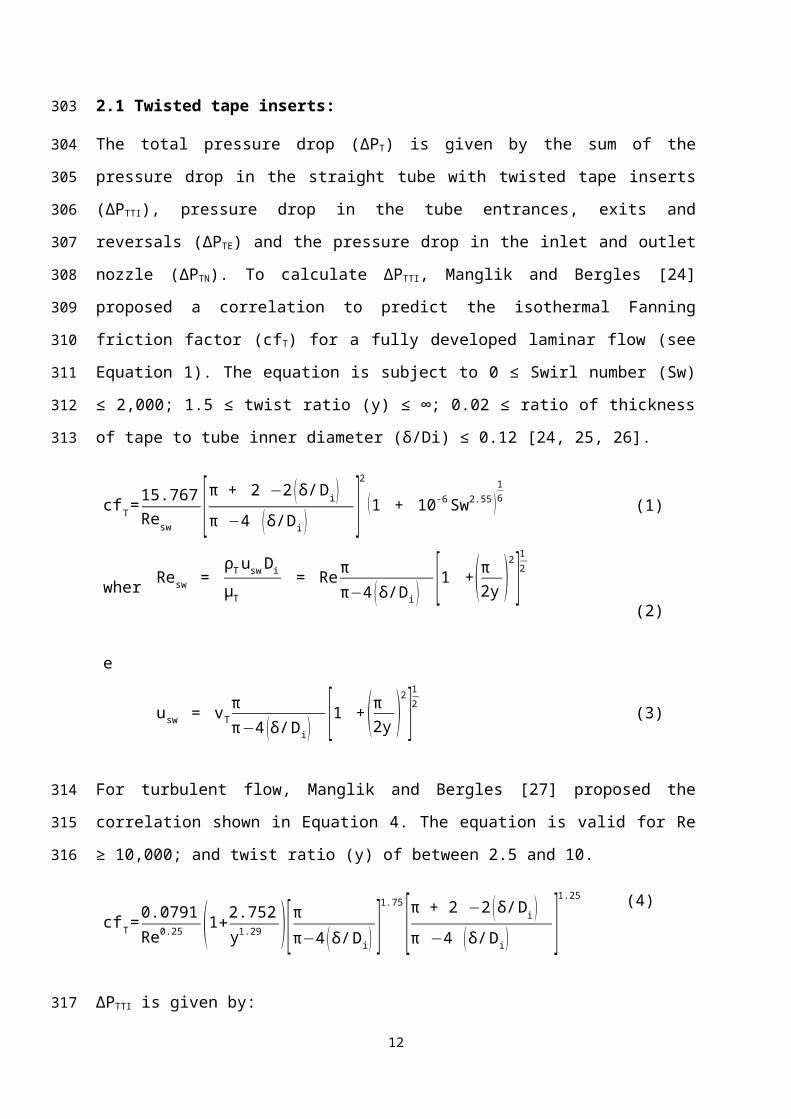
2.1 Twisted tape inserts:
The total pressure drop (ΔPT) is given by the sum of the pressure drop in the straight tube
with twisted tape inserts (ΔPTTI), pressure drop in the tube entrances, exits and reversals
(ΔPTE) and the pressure drop in the inlet and outlet nozzle (ΔPTN). To calculate ΔPTTI, Manglik
and Bergles [24] proposed a correlation to predict the isothermal Fanning friction factor (cfT)
for a fully developed laminar flow (see Equation 1). The equation is subject to 0 ≤ Swirl
number (Sw) ≤ 2,000; 1.5 ≤ twist ratio (y) ≤ ∞; 0.02 ≤ ratio of thickness of tape to tube inner
diameter (δ/Di) ≤ 0.12 [24, 25, 26].
cf T =15.767Resw [π + 2 −2 (δ/ Di )
π −4 (δ/ Di ) ]2
(1 + 10-6 Sw2.55 )16 (1)
wher
e
Resw = ρT usw Di
μT = Re π
π−4 ( δ/ Di ) [1 +(π2y )
2]12
(2)
usw = vTπ π−4 ( δ/Di ) [1 +(π
2y )2]
12 (3)
For turbulent flow, Manglik and Bergles [27] proposed the correlation shown in Equation 4.
The equation is valid for Re ≥ 10,000; and twist ratio (y) of between 2.5 and 10.
cfT =0.0791Re0.25 (1+2.752
y1.29 ) [ππ−4 ( δ/Di ) ]1.75[π + 2 −2 ( δ/Di )
π −4 (δ/ Di ) ]1.25 (4)
ΔPTTI is given by:
7
193
194
195
196
197
198
199
200
201
202
203
204
205
206
207
208
209
210
211

∆ PTTI =4 cf T(LDi )(
ρT vT2
2 ) (5)
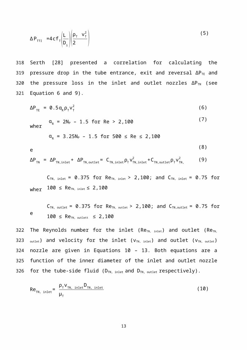
Serth [28] presented a correlation for calculating the pressure drop in the tube entrance, exit
and reversal ΔPTE and the pressure loss in the inlet and outlet nozzles ΔPTN (see Equation 6
and 9).
∆PTE = 0.5 αR ρT vT2 (6)
where
αR = 2NP – 1.5 for Re > 2,100 (7)
αR = 3.25NP – 1.5 for 500 ≤ Re ≤ 2,100 (8)
∆PTN = ∆PTN,inlet + ∆PTN,outlet = CTN,inlet ρT vTN,inlet2 + CTN,outlet ρT vTN,outlet
2 (9)
where
CTN, inlet = 0.375 for ReTN, inlet > 2,100; and CTN, inlet = 0.75 for 100 ≤ ReTN, inlet ≤ 2,100
CTN, outlet = 0.375 for ReTN, outlet > 2,100; and CTN,outlet = 0.75 for 100 ≤ ReTN, outlett ≤ 2,100
The Reynolds number for the inlet (ReTN, inlet) and outlet (ReTN, outlet) and velocity for the inlet
(vTN, inlet) and outlet (vTN, outlet) nozzle are given in Equations 10 – 13. Both equations are a
function of the inner diameter of the inlet and outlet nozzle for the tube-side fluid (DTN, inlet and
DTN, outlet respectively).
ReTN, inlet= ρT vTN, inlet DTN, inlet
μT
(10)
vTN, inlet = m T
ρT(π DTN, inlet2
4 ) (11)
ReTN, outlet = ρT vTN, outlet DTN, outlet
μT
(12)
vTN, outlet = mT
ρT(π DTN,outlet2
4 ) (13)
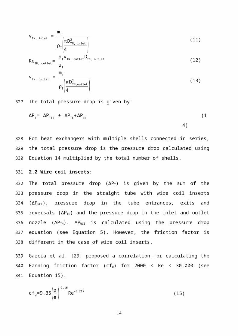
The total pressure drop is given by:
∆PT= ∆PTT I + ∆PTE+∆PTN (14)
8
212
213
214
215
216
217
218
219
For heat exchangers with multiple shells connected in series, the total pressure drop is the
pressure drop calculated using Equation 14 multiplied by the total number of shells.
2.2 Wire coil inserts:
The total pressure drop (ΔPT) is given by the sum of the pressure drop in the straight tube
with wire coil inserts (ΔPWCI), pressure drop in the tube entrances, exits and reversals (ΔPTE)
and the pressure drop in the inlet and outlet nozzle (ΔPTN). ΔPWCI is calculated using the
pressure drop equation (see Equation 5). However, the friction factor is different in the case
of wire coil inserts.
Garcia et al. [29] proposed a correlation for calculating the Fanning friction factor (cfW) for
2000 < Re < 30,000 (see Equation 15).
cfW =9.35(pe )
-1.16
Re-0.217 (15)
Ravigururajan and Bergles [30] proposed a correlation for calculating the Fanning friction
factor for 30,000 < Re < 250,000 in augmented tube with structured roughness (see Equation
16).
cfW = cfs {1 + [29.1 Rea1(eDi )
a2
(pDi )
a3
(α90 )
a4]1516 }
1615
(16)
where a1= 0.67 – 0.06(pDi ) – 0.49(α90 ) (17)
a2= 1.37 – 0.157(pDi ) (18)
a3= –1.66 x 10⁻⁶ Re – 0.33(α90 ) (19)
a4 = 4.59 + 4.11 x 10⁻⁶ Re – 0.15(pDi ) (20)
(α90 )= 2π
tan-1 π
(pDi )
(21)
Filonenko [31] defined a correlation for the smooth tube friction factor (cfs):
9
220
221
222
223
224
225
226
227
228
229
230
231
232
233

cfs = (1.58lnRe – 3.28 )-2 (22)
The total pressure drop is given by:
∆PT= ∆PWCI + ∆PTE+∆PTN (23)
Similar to twisted tape inserts, heat exchangers with multiple shells connected in series, the
total pressure drop is the pressure drop calculated in Equation 23 multiplied by the total
number of shells.
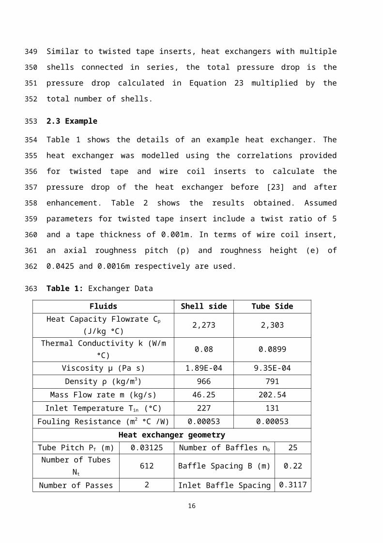
2.3 Example
Table 1 shows the details of an example heat exchanger. The heat exchanger was modelled
using the correlations provided for twisted tape and wire coil inserts to calculate the pressure
drop of the heat exchanger before [23] and after enhancement. Table 2 shows the results
obtained. Assumed parameters for twisted tape insert include a twist ratio of 5 and a tape
thickness of 0.001m. In terms of wire coil insert, an axial roughness pitch (p) and roughness
height (e) of 0.0425 and 0.0016m respectively are used.
Table 1: Exchanger Data
Fluids Shell side Tube Side
Heat Capacity Flowrate Cp (J/kg °C) 2,273 2,303
Thermal Conductivity k (W/m °C) 0.08 0.0899
Viscosity µ (Pa s) 1.89E-04 9.35E-04
Density ρ (kg/m3) 966 791
Mass Flow rate m (kg/s) 46.25 202.54
Inlet Temperature Tin (°C) 227 131
Fouling Resistance (m2 °C /W) 0.00053 0.00053
Heat exchanger geometryTube Pitch PT (m) 0.03125 Number of Baffles nb 25
Number of Tubes Nt 612 Baffle Spacing B (m) 0.22Number of Passes Np 2 Inlet Baffle Spacing Bin (m) 0.3117
Tube Length L (m) 6 Outlet Baffle Spacing Bout (m) 0.3117Tube Effective Length
Leff (m)5.9 Baffle cut Bc 20%
Tube Conductivity ktube
(W/m K)51.91
Inner Diameter of Tube-side Inlet Nozzle DT,inlet (m)
0.336
10
234
235
236
237
238
239
240
241
242
243
244
245
Tube Layout Angle 90Inner Diameter of Tube-side
Outlet Nozzle DT,outlet (m)0.336
Bundle ConfigurationStraight Tube
BundleInner Diameter of Shell-side
Inlet Nozzle DS,inlet (m)0.154
Tube Inner Diameter Di
(m)0.02
Inner Diameter of Shell-side Outlet Nozzle DS,outlet (m)
0.154
Tube Outer Diameter Do
(m)0.025
Shell-Bundle Diametric Clearance Lsb (m)
0.069
Shell Inner Diameter Ds
(m)0.97
Shell arrangement (series x parallel)
2 x 1
Table 2: Enhancement Results
Tube Side Shell side
hT (kW/m2 °C) ∆PT (kPa) hS (kW/m2 °C) ∆PS (kPa)
Base Case 1.58 95.23 1.91 69.09
Twisted Tape 2.64 130.32 1.91 69.09
Wire Coil 3.26 111.51 1.91 69.09
From the result shown in Table 2, the use of both enhancement techniques led to an increase
in the pressure drop by 36.9% for twisted tape and 17.1% for wire coil inserts. In this case,
the existing pumps might not be able to cope with the increase in pressure drop. This problem
can be solved by installing additional pumps either as replacements or in series with existing
ones or retrofitting the existing pumps. However, in retrofit, it might not be economic to
consider the installation of pumps with increased capacity. Therefore, presenting different
methods for mitigating the increase in pressure drop with enhancement is vital.
3 Pressure drop mitigation
The example studied in the previous section highlights the effect of heat transfer
enhancement on both heat transfer coefficient and pressure drop. Not only does the heat
transfer enhancement techniques used increase the heat transfer coefficient, but also the
pressure drop. In addition to installing a pump to cope with the increase in pressure drop,
other methods can be considered for pressure drop mitigation. Methods used in mitigating
pressure drop are discussed in more detail in the following sections.
11
246
247
248
249
250
251
252
253
254
255
256
257
258
259
260
3.1 Tube passes
Modifying the tube passes in existing heat exchangers is one way of reducing the pressure
drop. Reducing the tube passes in existing heat exchangers results in a decrease in the tube-
side flow velocity but the overall performance of the heat exchanger can still be improved
with the use of heat transfer enhancement. Examples of common tube passes used in the
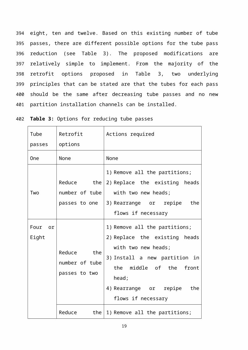
design of shell and tube heat exchangers are one, two, four, six, eight, ten and twelve. Based
on this existing number of tube passes, there are different possible options for the tube pass
reduction (see Table 3). The proposed modifications are relatively simple to implement. From
the majority of the retrofit options proposed in Table 3, two underlying principles that can be
stated are that the tubes for each pass should be the same after decreasing tube passes and no
new partition installation channels can be installed.
Table 3: Options for reducing tube passes
Tube passes Retrofit options Actions required
One None None
TwoReduce the number
of tube passes to one
1) Remove all the partitions;
2) Replace the existing heads with two new
heads;
3) Rearrange or repipe the flows if necessary
Four or
Eight
Reduce the number
of tube passes to two
1) Remove all the partitions;
2) Replace the existing heads with two new
heads;
3) Install a new partition in the middle of the
front head;
4) Rearrange or repipe the flows if necessary
Reduce the number
of tube passes to one
1) Remove all the partitions;
2) Replace the existing heads with two new
heads;
3) Rearrange or repipe the flows if necessary
12
261
262
263
264
265
266
267
268
269
270
271
272
Six or Ten
Reduce the number
of tube passes to two
Remove all partitions except the middle one
in the front head
Reduce the number
of tube passes to one
1) Remove all the partitions;
2) Replace the existing heads with two new
heads;
3) Rearrange or repipe the flows if necessary
Twelve
Reduce the number
of tube passes to
four
Remove some partitions and retain those in
the typical 4-tube-pass layout
Reduce the number
of tube passes to two
1) Remove all the partitions;
2) Replace the existing heads with two new
heads;
3) Install a new partition in the middle of the
front head;
4) Rearrange or repipe the flows if necessary
Reduce the number
of tube passes to one
1) Remove all the partitions;
2) Replace the existing heads with two new
heads;
3) Rearrange or repipe the flows if necessary
This technique is used in reducing the tube side pressure drop. Therefore, considering the
example heat exchanger provided in Table 1, the pressure drop after the application of heat
transfer enhancement can be reduced by modifying the tube passes. There are two tube passes
in this example heat exchanger. From Table 3, the only option available is to reduce the
number of tube passes from two to one. Table 4 shows the result obtained when this
procedure was applied.
Table 4: Result from tube pass reduction
Before Modification After Modification
hT (kW/m2 °C) ∆PT (kPa) hT (kW/m2 °C) ∆PT (kPa)
Base Case 1.58 95.23 0.905 21.26
13
273
274
275
276
277
278
279
Twisted Tape 2.64 130.32 1.51 42.23
Wire Coil 3.26 111.51 1.98 49.77
From Table 4, it can be noted that the heat transfer coefficient in the base case scenario
decreases as a result of the decrease in the number of tube passes. However, the decrease in
performance can be compensated for with the use of enhancement in particular. In this case, a
wire coil insert has been used, which was still able to provide a degree of enhancement
compared to the base case but at a lower pressure drop. In summary, this example shows that
modifying the number of tube passes can mitigate the increase in pressure drop with the use
of heat transfer enhancement. However, this comes at a penalty of decreased level of
enhancement when compared to the scenario where pressure drop is not considered.
3.2 Modification of shell arrangement
In retrofit, the presence of more than one shell in a heat exchanger allows for an opportunity
to reduce its pressure drop requirement. The total pressure drop of the heat exchanger is
dependent on the shell arrangement and the total number of shells. Different shell
arrangements have a significant impact on pressure drop. For example, for a two shell heat
exchanger, the shells can either be arranged in series or in parallel (see Figure 1). In the case
of the series arrangement of shells, the total pressure drop is the sum of pressure drop of both
shells. In the series arrangement, the entire flow goes through both shells resulting in pressure
drop and heat transfer coefficient that are relatively high. On the other hand, with parallel
arrangement, the total pressure drop is given by the maximum pressure drop in either of the
shells. With a parallel arrangement, the heat transfer coefficient and pressure drop are lower
as the flow going through each shell is lower than that of series arrangement.
14
280
281
282
283
284
285
286
287
288
289
290
291
292
293
294
295
296
297
298
299
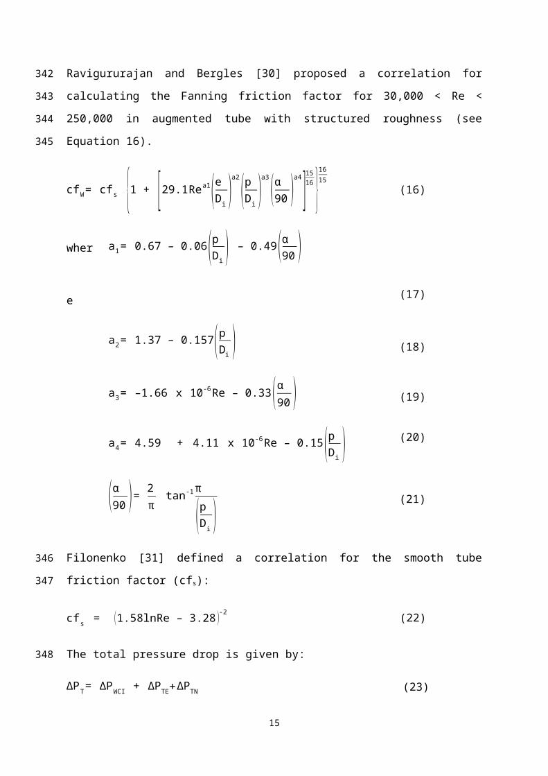
Figure 1: Shell arrangement
In the case where there are more than two shells in a heat exchanger, a mixed arrangement
can be used (see Figure 2). In this case, each shell has intermediate heat transfer coefficients
and pressure drops compared to the series and parallel arrangements.
Figure 2: Mixed arrangement (2series, 2 parallel)
This technique can be used in reducing both the shell and tube side pressure drop
requirement. Again, considering the example heat exchanger provided in Table 1, it is
assumed that the two shells are in series. Therefore, to reduce the pressure drop we can
modify the shell arrangement from series to parallel. A split ratio of 0.5 is assumed for both
the shell and tube side analysis. Tables 5 and 6 show the result obtained when this approach
was applied to reduce the shell and tube side pressure drop respectively.
Table 5: Shell side mitigation
Before Modification After Modification
15
300
301
302
303
304
305
306
307
308
309
310
311
312
313
hS (kW/m2 °C) ∆PS (kPa) hS (kW/m2
°C)
∆PS (kPa)
Base Case 1.91 69.09 1.21 18.92
Twisted Tape 1.91 69.09 1.21 18.92
Wire Coil 1.91 69.09 1.21 18.92
Table 6: Tube side mitigation
Before Modification After Modification
hT (kW/m2 °C) ∆PT (kPa) hT (kW/m2 °C) ∆PT (kPa)
Base Case 1.58 95.23 0.905 27.31
Twisted Tape 2.64 130.32 1.51 37.61
Wire Coil 3.26 111.51 1.98 45.16
The results show that modifying the shell arrangement resulted in a decrease in both the heat
transfer coefficients and the pressure drop for both cases. Also, the result obtained in Table 6
is the same as that obtained for reducing the number of tube passes from two to one (see
Table 4) in terms of heat transfer coefficients. This result is expected as the velocity of the
tube-side in both cases decreases by a factor of half. However, the pressure drop is different
from that of reducing the number of tube passes due to the tube-side entrance and exit
pressure drop losses, which is a function of the number of tube passes (see Equations 7 and
8).
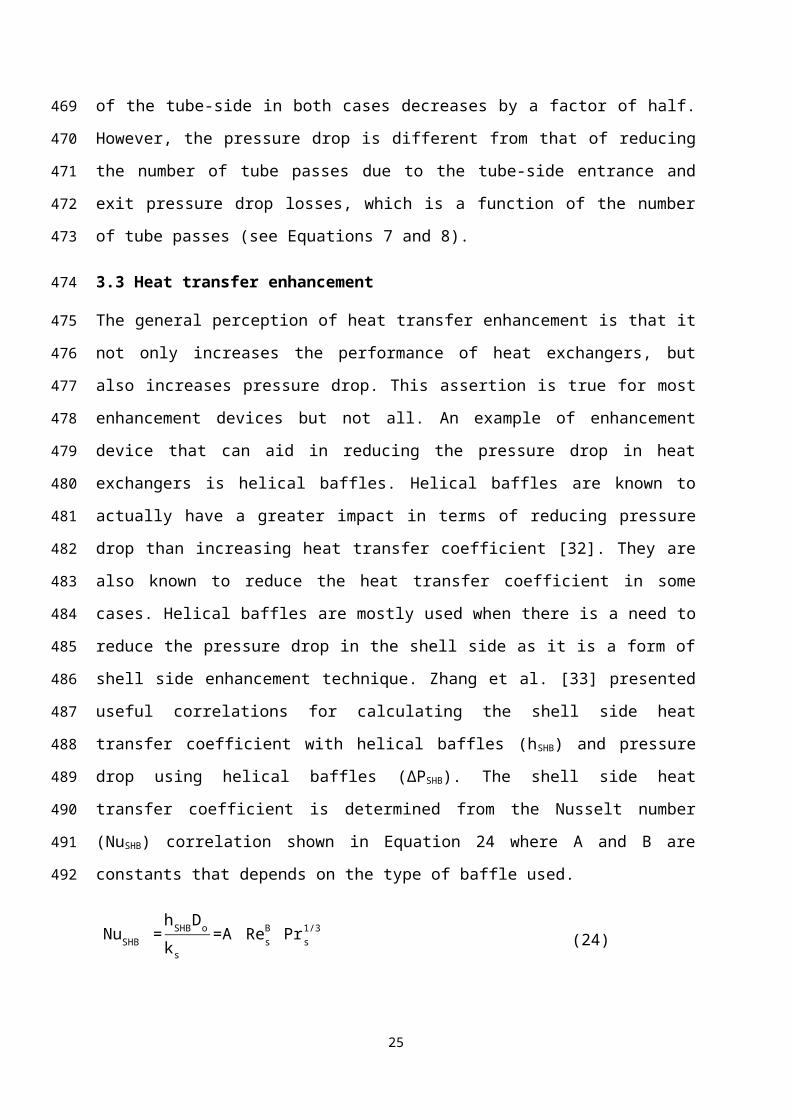
3.3 Heat transfer enhancement
The general perception of heat transfer enhancement is that it not only increases the
performance of heat exchangers, but also increases pressure drop. This assertion is true for
most enhancement devices but not all. An example of enhancement device that can aid in
reducing the pressure drop in heat exchangers is helical baffles. Helical baffles are known to
actually have a greater impact in terms of reducing pressure drop than increasing heat transfer
coefficient [32]. They are also known to reduce the heat transfer coefficient in some cases.
Helical baffles are mostly used when there is a need to reduce the pressure drop in the shell
side as it is a form of shell side enhancement technique. Zhang et al. [33] presented useful
correlations for calculating the shell side heat transfer coefficient with helical baffles (hSHB)
and pressure drop using helical baffles (ΔPSHB). The shell side heat transfer coefficient is
16
314
315
316
317
318
319
320
321
322
323
324
325
326
327
328
329
330
331
332
333

determined from the Nusselt number (NuSHB) correlation shown in Equation 24 where A and
B are constants that depends on the type of baffle used.
NuSHB =hSHBDo
ks=A Re s
B Prs1/3
(24)
where Res = Shell side Reynolds number =ρs u sDo
μs(25)
Pr=Shell side Prandtl number=Cpsμs
ks(26)
The friction factor (cfSHB) is dependent on the shell side Reynolds number, as shown in
Equation 27, where C and D are constants dependent on the baffle type.
cfSHB = C ResD (27)
The pressure drop for helical baffles can then be calculated using the correlation shown in
Equation 28. Values for each constant (A, B, C and D) are given in Table 7.
∆ PSHB = 2 cfSHB Nt L ρs us
2
X (28)
where X = √2 Ds tan β (29)
Table 7: Values of constants A, B, C and D [33]
Baffle type A B C D
Helical baffles, β = 20° 0.275 0.542 11.0 -0.715
Helical baffles, β = 30° 0.365 0.516 13.5 -0.774
Helical baffles, β = 40° 0.455 0.488 34.7 -0.806
Helical baffles, β = 50° 0.326 0.512 47.9 -0.849
The total pressure drop when helical baffles are used is the sum of the pressure drop in the
straight section with helical baffles and the pressure drop in the nozzles (ΔPSN).
∆PS = ∆PSHB +∆PSN (30)
17
334
335
336
337
338
339
340
341
342

For heat exchangers with multiple shells, the pressure drop calculated using Equation 30 is
multiplied by the total number of shells.
To examine the influence of helical baffles on heat transfer coefficient and pressure drop;
helical baffles are implemented in the example heat exchanger shown in Table 1. Table 8
confirms that helical baffles not only reduce the shell side pressure drop but also the heat
transfer coefficient. Based on this example, the best baffle type to use will be 30°, as the
degree of enhancement between this baffle and that at 40° is close, but the difference in
pressure drop is considerable.
Table 8: Application of helical baffles
Shell sidehS (kW/m2 °C) ∆PS (kPa)
Base Case 1.91 69.09
Helical baffles, β = 20° 0.848 67.87
Helical baffles, β = 30° 0.832 32.27
Helical baffles, β = 40° 0.748 37.23
Helical baffles, β = 50° 0.709 25.86
3.4 Other practical methods
Nie and Zhu [34] identified four other opportunities that can be applied in practice to tackle
pressure drop problems when looking at a HEN. The opportunities identified are as follows.
Option 1: Exploiting streams with spare pressure drop capacity:
This opportunity arises from the fact that in a given HEN, not every stream will have a
pressure drop constraint. Therefore, a certain amount of heat load can be shifted between
exchangers on constrained and unconstrained streams.
Option 2: Releasing pressure drop from existing heat exchangers on the same stream:
The shell arrangements of each heat exchanger on the stream can be manipulated to reduce
the pressure drop requirement of the stream. This releases the pressure drop and allows for
heat transfer enhancement techniques to be applied, while still maintaining the pressure
constraint of the stream. Also, if the shell arrangement of a heat exchanger is modified from
series to parallel, this not only reduces the pressure drop requirement, but also increases the
18
343
344
345
346
347
348
349
350
351
352
353
354
355
356
357
358
359
360
361
362
363
364
performance of heat exchangers located downstream. As such, the overall energy
performance is improved.
Option 3: Modifying the existing pumps to increase the allowable pressure drop requirement:
This is often not a desirable option in retrofit due to the cost associated with pump
modification. However, if this is an option the pump capacity can be improved by methods
such as increasing the impeller size or increasing the rotating speed of the pump. This
increases the discharge pressure and the allowable pressure drop of the HEN.
Option 4: Exploiting utility conditions:
Increasing the duty of a heat exchanger in an existing network not only results in target
temperature violations but also additional heat transfer area requirements in downstream
exchangers due to the decrease in driving force. Ordinarily, additional heat transfer area can
be added to existing heat exchangers in order to maintain the energy balance. However, this
might result in an increase in the pressure drop beyond the allowable limit of the existing
pump. With this method, utilities are either replaced with higher temperature utility or one
with a higher heat transfer coefficient, instead of increasing the heat transfer area of existing
heat exchangers.
In addition to the practical methods presented by Nie and Zhu [34], other methods can be
used in mitigating pressure drop in the shell and tube sides. In terms of shell side pressure
drop mitigation, the baffle cut, baffle spacing and tube pitch can be increased. Other methods
include changing the tube pitch configuration from triangular to square or rotated to in-line or
use an alternative baffle design. For tube side mitigation, the tube length can be decreased;
the shell diameter and tube diameter can be increased. In summary, it is important to point
out that although these methods might be able to mitigate pressure drop requirement, it is
always advisable to explore the effect of performing these modifications in terms of cost.
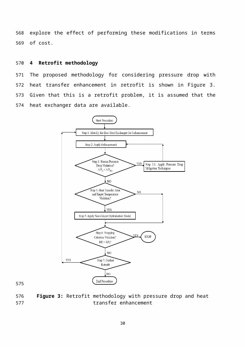
4 Retrofit methodology
The proposed methodology for considering pressure drop with heat transfer enhancement in
retrofit is shown in Figure 3. Given that this is a retrofit problem, it is assumed that the heat
exchanger data are available.
19
365
366
367
368
369
370
371
372
373
374
375
376
377
378
379
380
381
382
383
384
385
386
387
388
389
390
391
392
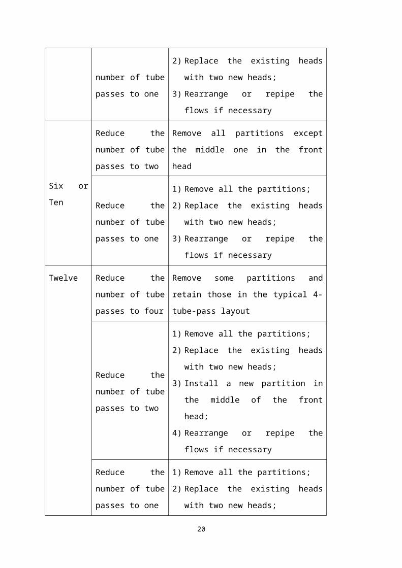
Figure 3: Retrofit methodology with pressure drop and heat transfer enhancement
Step 1: Given the base case heat exchanger data, the first step is the identification of the best
heat exchanger to enhance. This procedure is a two-step approach as described in [22, 23].
The first step is the identification of heat exchangers on a utility path. For simple
networks, heat exchangers on a utility path can be identified by inspection. However,
for complex networks, a more systematic method is required i.e. the Incidence Matrix
Approach is used. The Incidence Matrix characterises a network as a number of
streams by number of exchangers matrix where the rows represent the number of
process and utility streams and the columns represents a number of process and utility
exchangers. Figure 4 shows an example network used for illustrating the application
of Incidence Matrix Approach for identifying utility paths. From Figure 4, If a heat
exchanger removes heat from a stream and supplies heat to another, a value of +1 and
20
393
394
395
396
397
398
399
400
401
402
403
404
405

-1 are added to signify the stream from which heat is removed and added respectively.
The utility path is dependent on the column vector P added to the Incidence Matrix.
As such, a value of +1 and -1 must added under the column vector to signify the hot
and cold utility respectively (see Table 9). To identify heat exchangers on a utility
path, the column vector P is used. A linear combination of the reduced incidence
matrix gives this. The matrix is reduced by performing row operations to ensure that
all entries below the first non-zero entry of each row are zero (see Table 10). Linear
combination is based on utility path analysis, which states that if a certain amount of
heat is added to a heater that same amount must be subtracted from a heat exchanger
on a utility path as that heater, added to the next, subtracted from the next until finally
that same amount of heat load is added to a cooler on the same utility path as that
heater. Therefore, the column profile identified by performing the plus-minus analysis
must be equal to the column vector P. Figures 5 and 6 shows the paths identified
based on the example network.
Figure 4: Example Network
Table 9: Initial Incidence Matrix
S/E 1 2 3 4 C1 C2 H P
1 0 0 +1 0 +1 0 0 0
2 0 0 0 +
1
0 +1 0 0
3 +
1
+1 0 0 0 0 0 0
4 0 -1 -1 0 0 0 0 0
5 -1 0 0 -1 0 0 -1 0
HU 0 0 0 0 0 0 +1 +1
CU 0 0 0 0 -1 -1 0 -1
21
406
407
408
409
410
411
412
413
414
415
416
417
418
419
420
421
422

Table 10: Reduced Incidence Matrix
S/E 1 2 3 4 C1 C2 H P
1 0 0 +1 0 +1 0 0 0
2 0 0 0 +
1
0 +1 0 0
3 +
1
+1 0 0 0 0 0 0
4 0 -1 0 0 +1 0 0 0
5 0 0 0 0 +1 +1 -1 0
HU 0 0 0 0 0 0 +1 +1
CU 0 0 0 0 0 0 0 0
Figure 5: First Utility Path
Figure 6: Second Utility Path
22
423
424
425
426
427

In the second step, either sensitivity analysis [20, 21 and 22] or the area ratio
approach [23] can be used in determining the best heat exchanger to enhance. The
fundamental idea is to be able to evaluate the energy saving potential of candidate
heat exchangers i.e. exchangers on a utility path. In this paper, only area ratio
approach is explored. A way of reducing the energy consumption in a network is by
adding heat transfer area to existing heat exchangers (see Equation 31). However, this
work focuses only on the use of heat transfer enhancement for energy recovery.
Assuming enhancement can completely accommodate the need for additional area to
obtain the same degree of energy savings, an expression for area ratio can be derived
(see Equations 32 and 33)
Q = U(A +∆A)∆TLMFT (31)
Q = UEA∆TLMFT (32)
AR =A(A +∆A )
= U UE (33)
Based on Equation 33, the best heat exchanger to enhance is one with the smallest
area ratio as this signifies the heat exchanger that can provide the greatest degree of
enhancement relative to its base case value.
Step 2: In the second step, the chosen enhancement technique is applied to the best heat
exchanger identified in Step 1.
Step 3: The stream pressure drop is then checked after enhancement. If there are pressure
drop violations, the mitigation techniques described in Section 3 are applied (Step 3.1). If not
continue to Step 4. The decision on what technique to apply depends on the stream that is
constrained. For example, if the shell side is constrained, helical baffles or changing the shell
arrangements could be considered. If on the other hand, the constraint is on the tube side,
then reduction in the number of tube passes or change in the shell arrangement could be
considered. Given the new exchanger geometry and data, the new heat transfer coefficient
and pressure drop for the new base case and enhanced conditions could be determined. In
situations where there is more than one mitigation option, a ranking criterion is required to
determine the best modification option. The ranking criterion (SF) is defined as the change in
pressure drop with respect to the change in the degree of enhancement before and after
applying modifications (Equation 34). The best option is one with the smallest selection
23
428
429
430
431
432
433
434
435
436
437
438
439
440
441
442
443
444
445
446
447
448
449
450
451
452
453
454

factor, as this signifies the modification that can still provide a higher degree of enhancement
with the lowest pressure drop penalty.
SF =(∆PN,E – ∆PN
∆PB,E – ∆PB)(UB,E – UB
UN,E – UN) (34)
Step 4: After satisfying the pressure drop constraint, the network is checked for heat transfer
area and target temperature constraint violations. This is essential, as the aim is to apply heat
transfer enhancement without the need for additional heat transfer area, while ensuring
energy balance is maintained. If the constraints are not violated, continue to Step 6 otherwise
continue to Step 5.
Step 5: In case of constraint violations, a non-linear optimisation model can be applied. The
non-linear optimisation model is similar to that presented in [22, 23]. However, it has been
modified to take into account the cost associated with the application of the mitigation
techniques. The objective function of the non-linear optimisation model used is still to
maximise the retrofit profit (RP) (see Equation 35).
RP=UC B−[UC E+ ∑ex∈ EX
RC ex ] (35)
In this case, the retrofit cost includes the cost of modifications and is given in Equation 36
where, ECex is the enhancement cost of exchangers, ACex is the additional area cost, BCex is
the cost of bypass, and MCex is the modification cost. Factors, EF, AF, BF, and MF are
assigned to each individual cost. If a heat exchanger is enhanced, additional area is required,
bypass is required or modifications are made to the exchanger geometry, the values of EF,
AF, BF, and MF are one otherwise zero. Equations 37 and 38 are used in calculating the
utility cost before and after enhancement where CCU and CHU are the yearly cost parameters
for cold and hot utility, QB and QE are the duties before and after enhancement and OT is the
payback operating time.
RCex=ECex×EF ex+AC ex× AF ex+BC ex×BF ex+MCex×MFex∀ ex∈EX (36)
UC B=OT ×[CCU× ∑ex∈EX CU
QB , ex+CHU × ∑ex∈EX HU
QB ,ex ]
(37)
UC E=OT ×[CCU × ∑ex∈EX CU
QE ,ex+CHU × ∑ex∈ EX HU
QE ,ex ]
(38)
24
455
456
457
458
459
460
461
462
463
464
465
466
467
468
469
470
471
472
473
474
475
The aim of the optimisation model is to be able to apply heat transfer enhancement without
the need for additional heat transfer area and ensuring the target temperatures of all streams
are met (see Equations 39 – 41). Equations 39 to Equation 41 represent the constraints for
heat transfer area requirement, and target temperature constraints for all cold and hot streams,
CS and HS. Aex and AE represent the heat transfer area of all process heat exchangers before
and after the application of enhancement. TCOSCS and THOSHS represent the cold and hot
outlet stream temperatures.
Aex=A E∀ ex∈ EXE (39)
TCOS i ,CS=TCOS f ,CS∀CS (40)
THOSi , HS=THOSf , HS∀HS (41)
Variables used in this model are the overall heat transfer coefficients of all process heat
exchangers, subject to this value not exceeding the maximum determined based on the
exchanger geometry after enhancement. The duty of all heat exchangers on a utility path is
another variable used in this model. It is important to point out that although the overall heat
transfer coefficients of heat exchangers not on a utility path are varied, this is done at
constant heat exchanger duty.
Step 6: Given that the retrofit objective is to maximise the retrofit profit, after the application
of the non-linear optimisation model, if the retrofit profit before enhancement is greater than
that after, the procedure is stopped. This means that the profit obtained from applying
enhancement is less than the cost of retrofit. As such, it is uneconomic. If this is not the case,
proceed to Step 7.
Step 7: There might be more than one heat exchanger that can improve energy recovery. If
so, other candidate heat exchangers are sorted and the procedure is repeated. If all potential
for energy recovery has been explored, the procedure can be terminated.
5 Case Study
The case study shown in Figure 7 depicts a simplified crude-oil pre-heat train [22, 23]. Table
11 shows the data for each process heat exchanger in the network. The objective is to present
a retrofit design with the maximum retrofit profit while minimising the energy consumption
of the hot utility (exchanger 12) and maintaining the pressure drop, heat transfer area and
25
476
477
478
479
480
481
482
483
484
485
486
487
488
489
490
491
492
493
494
495
496
497
498
499
500
501

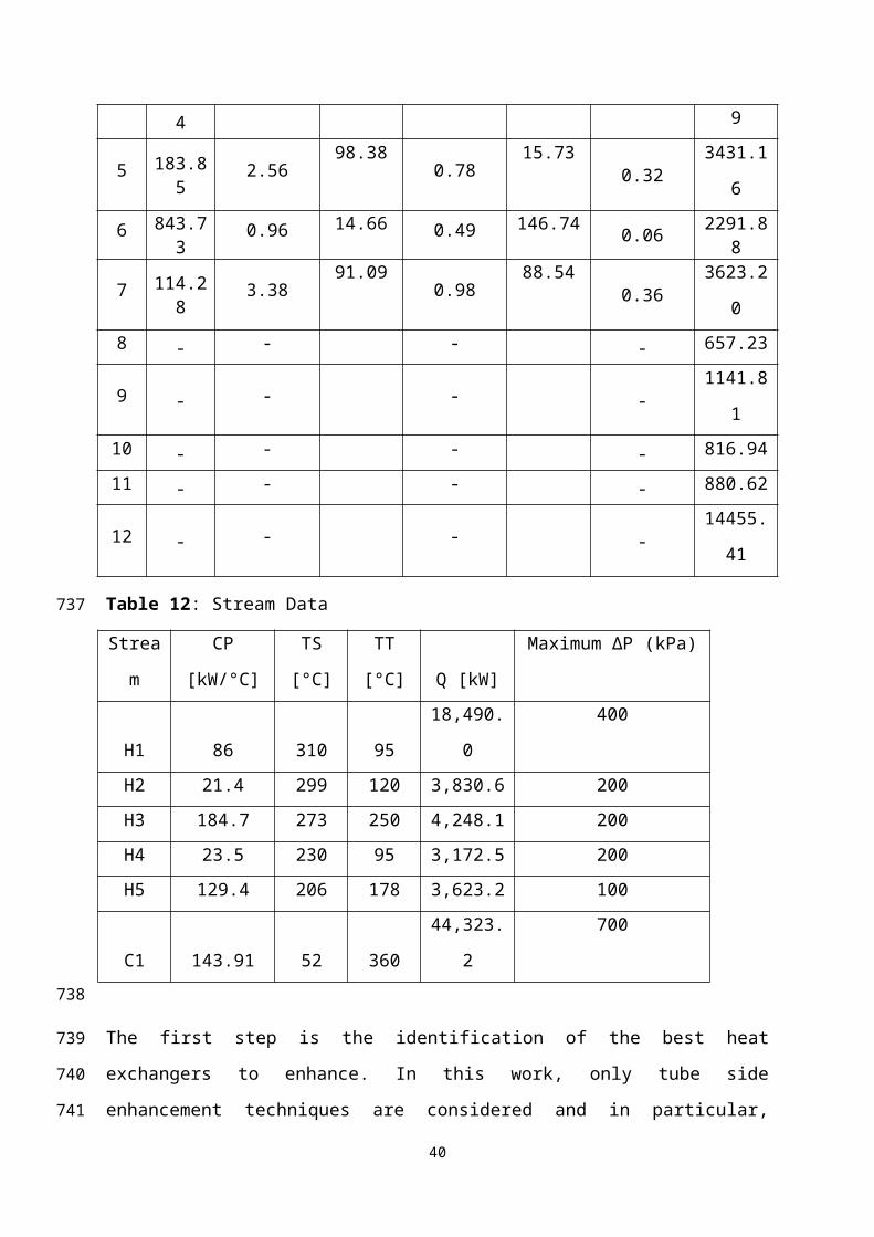
target temperature constraints in the network. Table 12 shows the stream data for the case
study, including the maximum pressure drop of each process stream in the HEN.
Figure 7: Case study
Table 11: Original Heat Exchanger Data
Ex. A (m2) hs
(kW/m2°C)∆PS
(kPa)hT
(kW/m2°C)∆PT
(kPa)U
(kW/m2°C)Q (kW)
1 396.72 2.07 78.49 1.33 167.29 0.52 6141.33
2 545.45 2.31 100.80 1.40 131.40 0.48 6134.83
3 633.85 4.54 75.76 0.78 73.43 0.16 5556.61
4 354.64 1.27 4.27 0.62 45.38 0.10 2688.79
5 183.85 2.56 98.38 0.78 15.73 0.32 3431.16
6 843.73 0.96 14.66 0.49 146.74 0.06 2291.887 114.28 3.38 91.09 0.98 88.54 0.36 3623.20
8 - - - - 657.23
9 - - - - 1141.81
10 - - - - 816.94
11 - - - - 880.62
12 - - - - 14455.41
Table 12: Stream Data
Stream CP [kW/°C] TS [°C] TT [°C] Q [kW] Maximum ∆P (kPa)
H1 86 310 95 18,490.0 400
H2 21.4 299 120 3,830.6 200
26
502
503
504
505
506
507

H3 184.7 273 250 4,248.1 200
H4 23.5 230 95 3,172.5 200
H5 129.4 206 178 3,623.2 100
C1 143.91 52 360 44,323.2 700
The first step is the identification of the best heat exchangers to enhance. In this work, only
tube side enhancement techniques are considered and in particular, twisted tape inserts are
used, as they brought about the largest degree of enhancement in all candidate process heat
exchangers. The geometric details of all candidate heat exchangers are given in Table 13. The
area ratio approach [23] is used in determining the enhancement sequence for this case study.
Table 14 shows the results obtained for each candidate heat exchanger. It is important to
point out that results for Exchanger 7 are not provided as it is the only process heat exchanger
not on a utility path. From Table 14, the best heat exchanger for enhancement is Exchanger 5,
as it has the smallest area ratio (i.e. signifies the heat exchanger that can accommodate for the
greatest increase in heat transfer area, and as such greatest decrease in utility consumption).
After enhancing Exchanger 5 the pressure drop on stream C1 is then checked for pressure
drop violation. Applying enhancement to Exchanger 5, results in an increase in its tube side
pressure drop from 15.73kPa to 37.67kPa. Initially, the total pressure drop of stream C1 was
668.51kPa. After enhancement, this value increases to 690.45kPa, which is below the
maximum allowable pressure drop in stream C1. Therefore, the next step in the retrofit
process is to check for heat transfer area and target temperature violations.
Enhancing Exchanger 5 resulted in a decrease in the driving force for Exchanger 1. At
constant duty, additional heat transfer area is required in Exchanger 1 to maintain the target
temperatures. Therefore, the non-linear optimisation model is applied. The optimisation was
carried out using the LINDO system What’s Best global solver [35]. Table 15 shows the cost
data for the utilities and cost of modifications. Table 16 shows the result obtained after
enhancing Exchanger 5 and applying the non-linear optimisation model. From Table 16,
enhancing exchanger 5 can bring about a total retrofit profit of ~3% of the initial utility cost
of $5,801,395.
Table 13: Detailed exchanger geometry
Heat exchanger Ex.1 Ex.2 Ex.3 Ex.4 Ex.5 Ex.6
27
508
509
510
511
512
513
514
515
516
517
518
519
520
521
522
523
524
525
526
527
528
529
530
531
532
533

geometryPT (m) 0.025 0.025 0.025 0.025 0.025 0.025
Nt 1032 985 1192 798 665 985Np 4 2 2 2 2 2
L (m) 6.4 9.3 8.5 7.4 4.4 13.6
ktube (W/m°C) 51.91 51.91 51.91 51.91 51.91 51.91
Tube Layout Angle 90 90 90 90 90 90
Di (m) 0.015 0.015 0.016 0.016 0.016 0.016
Do (m) 0.019 0.019 0.020 0.020 0.020 0.020
Ds (m) 1.02 1.00 1.10 0.90 0.82 1.00
nb 41 41 41 41 41 41
B (m) 0.3 0.3 0.3 0.3 0.488 0.25
Bin (m) 0.127 0.127 0.127 0.127 0.488 0.127
Bout (m) 0.127 0.127 0.127 0.127 0.488 0.127
Bc 20% 20% 20% 20% 25% 20%
DT,inlet (m) 0.1023 0.1023 0.1023 0.1023 0.3048 0.1023
DT,outlet (m) 0.1023 0.1023 0.1023 0.1023 0.3048 0.1023
DS,inlet (m) 0.079 0.079 0.079 0.079 0.3048 0.079
DS,outlet (m) 0.079 0.079 0.079 0.079 0.3048 0.079
Lsb (m) 0.074 0.074 0.071 0.071 0.041 0.071
Table 14: Area Ratio Result
Exchangers U (kW/m2°C) UE(kW/m2°C) AR
1 0.517 0.669 0.7732 0.475 0.597 0.7953 0.158 0.198 0.7984 0.0963 0.108 0.8915 0.325 0.448 0.7256 0.610 0.674 0.905
Table 15: Cost Data
Utility Cost Data Retrofit Cost Data
Hot Utility Cost: 400 ($/kW y) Cost of Inserts: 500 + 10*A ($)
Cold Utility Cost: 5.5 ($/kW y) Implementing By-Pass: 500 ($)
Cost of Increasing Heat Exchanger Area: 4000 + 200*A
($)
28
534
535
Cost of modifying shell arrangement: 10,000($)
Cost of modifying tube passes: 5,000 ($)
Table 16: Results after enhancing Exchanger 5
Retrofit Cost
Enhancement $2,338
Modification for Pressure Drop Mitigation
$0
Increasing Area $0
Implementing By-pass $500
Total Cost $2,838
Retrofit Profit
Utilities Savings $178,076
Net Saving (Utility Savings - Total Cost)
$175,238 (~3.0% of initial utility cost)
The next step is to explore other opportunities for energy recovery. The next candidate heat
exchanger for enhancement is Exchanger 1. Applying tube side enhancement to Exchanger 1
not only results in an increase of its overall heat transfer coefficient from 0.52 kW/m2°C to
0.67 kW/m2°C, but also the pressure drop from 167.29kPa to 169.25kPa. The total pressure
drop of stream C1 has now increased to 692.41kPa. Again this is below the maximum
allowable pressure drop, and as such the retrofit procedure can proceed to the next step which
is dealing with heat transfer area and target temperature violations. The final result obtained
after enhancing Exchanger 1 is given in Table 17.
Table 17: Results after enhancing Exchangers 5 and 1
Retrofit Cost
Enhancement $8,448
Modification for Pressure Drop Mitigation
$0
Increasing Area $0
Implementing By-pass $1,500
Total Cost $9,948
Retrofit Profit Utilities Savings (relative to initial utility cost)
$321,924
Net Saving (Utility Savings - Total $311,976 (~5.4% of
29
536
537
538
539
540
541
542
543
544
545
Cost) initial utility cost)
The procedure is repeated for the next best heat exchanger i.e. Exchanger 2. In the case of
Exchanger 2, the pressure drop after enhancement increased from 131.40kPa to 163.31kPa.
This increased the total pressure drop of Stream C1 to a value of 724.32kPa. Therefore,
pressure drop mitigation techniques must be applied. Exchanger 2 has two shells arranged in
series and two tube passes. In this case, there are two options available i.e. reducing the
number of tube passes from two to one and changing the shell arrangement from series to
parallel. A split fraction of 0.5 is assumed for the case of changing shell arrangement. In this
case, the selection of the best modification is based on the ranking criterion (SF). From the
result shown in Table 18, the modification of the shell arrangement is the best, as it has the
lowest value for SF.
30
546
547
548
549
550
551
552
553
554
555
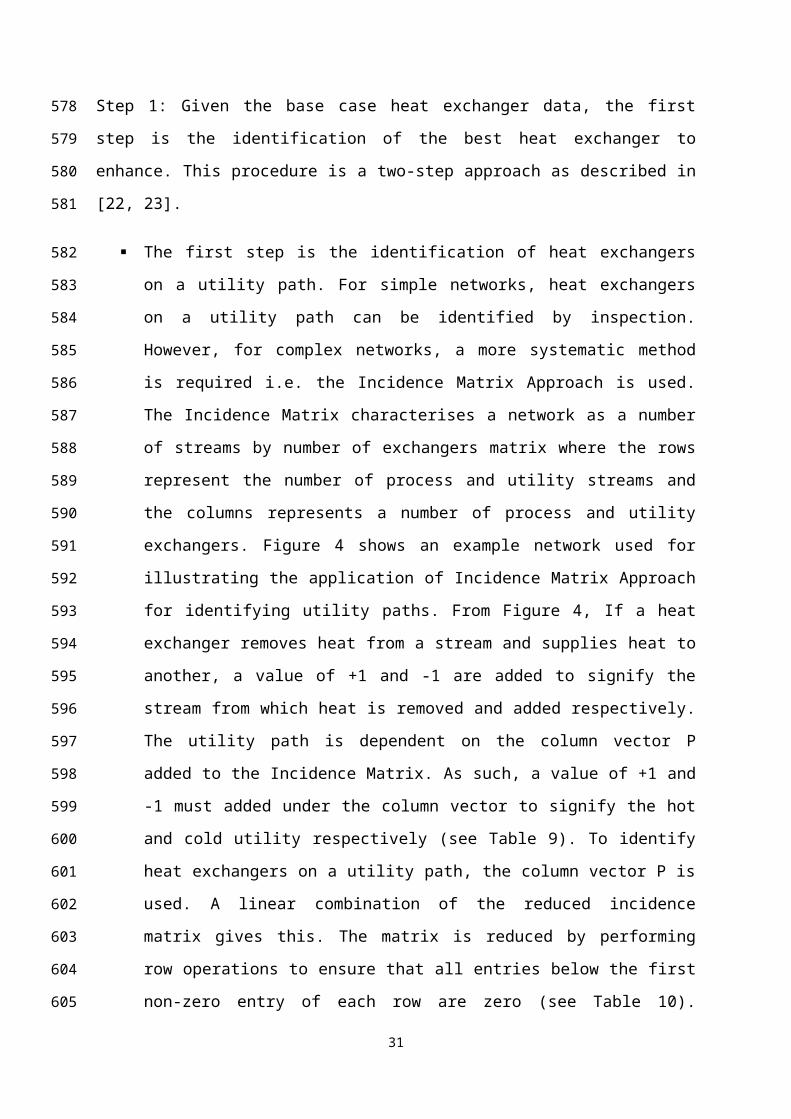
Table 18: Modification of Exchanger 2
Base Case After ModificationSFUB
(kW/m2°C)UB,E
(kW/m2°C)∆PB (kPa)
∆PB ,E (kPa)
UN
(kW/m2°C)UN,E
(kW/m2°C)∆PN (kPa)
∆PN ,E (kPa)
Original
Design0.475 0.597 131.40 163.31 - - - - -
Tube pass
reduction
(two to one)
0.475 0.597 131.40 163.31 0.356 0.490 113.80 125.48 0.33
Shell
Modification
(series to
parallel)
0.475 0.597 131.40 163.31 0.361 0.494 33.77 43.22 0.27
31
556
557
558
559
560
The modification is applied based on the degree of enhancement after shell
modification to Exchanger 2 is applied. The network is checked for violations and if
there are any, the violations are corrected using the non-linear optimisation model.
The retrofit profit obtained after enhancing Exchanger 2 (see Table 19) is less than
that before. Therefore, the result obtained is discarded, as it is not economic to apply
enhancement. The final details of all heat exchangers after enhancement with
pressure drop considerations are given in Table 20.
Table 19: Enhancement Result after Enhancing Exchanger 5, 1 and 2
Retrofit Cost
Enhancement $14,323
Modification for Pressure Drop Mitigation
$10,000
Increasing Area $0
Implementing By-pass $1,500
Total Cost $25,823
Retrofit Profit
Utilities Savings (relative to initial utility cost)
$242,017
Net Saving (Utility Savings - Total Cost)
$216,194 (~3.9% of initial utility cost)
Table 20: Final Heat Exchanger Data
Ex A (m2) UF
(kW/m2°C)∆TLM (°C) FT Q (kW) ∆PT
(kPa)∆PS
(kPa)1 396.72 0.67 28.29 0.88 6104.73 169.25 78.49
2 545.45 0.48 29.00 0.82 6162.68 131.40 100.80
3 633.85 0.16 62.80 0.88 5561.54 73.43 75.76
4 354.64 0.10 84.06 0.94 2688.32 45.38 4.27
5 183.85 0.45 53.53 0.96 4230.13 37.67 98.38
6 843.73 0.06 46.00 0.97 2291.21 146.74 14.66
7 114.28 0.36 88.76 0.97 3623.20 88.54 91.09
8 - - - - 661.04 - -9 - - - - 1142.28 - -
32
561
562
563
564
565
566
567
568
569
570

10 - - - - 17.97 - -11 - - - - 881.29 - -12 - - - - 13661.52 - -
A comparative analysis (see Figure 8) shows that with pressure drop considerations,
only a decrease in utility consumption of ~5.5% can be achieved, compared to the
7% achieved without pressure drop consideration [22, 23]. Compared to the result
obtained without pressure drop [22, 23], the retrofit profit obtained with pressure
drop consideration represents a decrease of ~18.5%. This result was obtained even
though the retrofit cost with pressure drop was considerably lower than that without.
The higher retrofit profit without pressure drop is obtained as there was more
opportunity for increasing energy recovery by enhancing more candidate heat
exchangers.
Figure 8: Comparative Analysis
6 Conclusions
This work presents a new systematic approach for pressure drop considerations with
heat transfer enhancement in retrofit. The approach is based on a combination of
heuristics and optimisation to meet the retrofit target. The method first identifies the
heat exchangers for enhancement. Then the network is checked for pressure drop
33
571
572
573
574
575
576
577
578
579
580
581
582
583
584
585
586

violations. If there are violations, pressure drop mitigation techniques are used to
solve the problem. For tube side pressure drop violations, modifying the number of
tube passes and shell arrangement can be considered. In terms of shell side
violations, the use of helical baffles or the modification of shell arrangement can be
considered. In cases where there is no pressure drop violations, other constraints
such as heat transfer area and target temperature constraints are examined. Heat
transfer area and target temperature violations are corrected using a non-linear
optimisation model. The aim in retrofit is not only to present a feasible design that
incorporates all network constraints, but also an economic design. Therefore, a
stopping criterion for the retrofit profit is included in the methodology. The
procedure is stopped when the application of enhancement, subject to all constraints
being met, becomes uneconomic. The effectiveness of the approach is demonstrated
with the case study presented in this paper. The results of the approach are compared
against that without pressure drop considerations. The results show that the energy
savings and retrofit profit decreases with pressure drop considerations due to the
constraint on the maximum degree of enhancement that can be applied so as not to
violate the stream pressure drop.
Nomenclature
Symbols Definitions Units
A Heat transfer area m2
AR Area ratio -
AC Area cost $
AF Area factor -
B Baffle spacing m
BC Baffle cut -
B¿ Inlet baffle spacing m
Bout Outlet baffle spacing m
BC Bypass cost $
BF Bypass factor -
c fS Smooth tube friction factor -
34
587
588
589
590
591
592
593
594
595
596
597
598
599
600
601
602
603
604
c fT Tube-side friction factor for twisted tape -
c fW Tube-side friction factor for wire coil -
CP Heat capacity Jkg-1°C-1
CCU Cost parameter for cold utility $/y
cf SHB friction factor for helical baffles -
CHU Cost parameter forhot utility $/y
Di Tube inner diameter m
Do Tube outer diameter m
DS Shell inside diameter m
DSN ,inlet Inner diameter of the inlet nozzle for the shell-side fluid m
DSN ,outlet Inner diameter of the outlet nozzle for the shell-side fluid m
DTN ,inletInner diameter of the inlet nozzle for the tube-side fluid m
DTN ,outletInner diameter of the outlet nozzle for the tube-side fluid m
e Wire diameter m
U E Enhanced overall heat transfer coefficient kWm-2°C-1
U F Final overall heat transfer coefficient kWm-2 °C-1
EC Enhancement cost $
EF Enhancement Factor -
FT Correction factor -
hS Shell-side heat transfer coefficient kWm-2°C-1
hSHB Shell-side heat transfer coefficient with helical baffles kWm-2°C-1
hT Tube-side heat transfer coefficient kWm-2°C-1
k Fluid thermal conductivity kWm-1°C-1
k s Shell thermal conductivity kWm-1°C-1
k tube Tube thermal conductivity kWm-1°C-1
L Length m
Leff Effective tube length m
m Mass flowrate kgs-1
35

MC Modification cost $
MF Modification factor -
mT Mass flowrate on the tube-side kg s-1
NB Number of baffles -
N P Number of tube passes -
OT Operating time y
p Roughness pitch m
pT Tube pitch m
Q Heat duty kW
RC Retrofit cost $
RP Retrofit Profit $
SF Selection factor -
TCOS Cold outlet temperature of stream °C
THOS Hot outlet temperature of stream °C
TS Supply temperature °C
TT Target temperature °C
U B Base overall heat transfer coefficient kWm-2°C-1
U B,E Base overall heat transfer coefficient after enhancement kWm-2°C-1
U N New overall heat transfer coefficient kWm-2°C-1
U N , E New overall heat transfer coefficient after enhancement kWm-2°C-1
uS Mean fluid velocity inside the shell ms-1
uSW Effective swirl velocity ms-1
uT Mean fluid velocity inside the tubes ms-1
UC Utility cost $
U E Enhanced overall heat transfer coefficient kWm-2°C-1
U F Final overall heat transfer coefficient kWm-2 °C-1
vTN , inletvelocity of the inlet nozzle for the tube-side fluid ms-1
vTN , outletvelocity of the outlet nozzle for the tube-side fluid ms-1
y Twist ratio -
36

∆ PB Base total pressure drop Pa
∆ PB, E Base total pressure drop after enhancement Pa
∆ PN New total pressure drop Pa
∆ PN , E New total pressure drop after enhancement Pa
∆ PS Total shell-side pressure drop Pa
∆ PSHB Total shell-side pressure drop using helical baffles Pa
∆ PSN Pressure drop in shell side nozzles Pa
∆ PT Total tube-side pressure drop Pa
∆ PTE Pressure drop in the tube entrances, exits and reversal Pa
∆ PTN Pressure drop in tube side nozzles Pa
∆ PTTI Pressure drop in the straight tubes with twisted tapes Pa
∆ PWCI Pressure drop in the straight tubes with wire coil Pa
∆T LM Log Mean Temperature Difference °C
Greek letters
μ Viscosity Pa s
ρ Fluid density kg m−3
δ Tape thickness m
β Helical baffles angle type °
α Function of number of tube passes -
Dimensionless groups:
Nu :Nusselt number=hDi
k
Pr :Prandtl number=Cp μk
ℜ:Reynolds number=ρu Di
μ
Sw :Swirl number= ℜ√ y
ππ−4 (δ /Di ) [1+( π
2 y )2]
12
37
605
606

Subscripts:
B Base
CS Cold stream
CU Cold utility
E Enhanced
ex, EX Exchanger
F Final
HS Hot stream
HU Hot utility
I Initial
N New
S Shell
SHB Shell helical baffles
T Tube
TT Twisted Tape
WC Wire coil
References
[1] Tjoe, T., and Linnhoff, B. (1986). Using pinch technology for process retrofit.
Chemical Engineering, 93(8), 47-60.
[2] Shokoya, C. G., and Kotjabasakis, E. (1991). Retrofit of heat exchanger networks
for bebottlenecking and energy savings. PhD Thesis, University of Manchester,
Institute of Science and Technology.
[3] Carlsson, A., Franck, P. A., and Berntsson, T. (1993). Design better heat
exchanger network retrofits. Chemical Engineering Progress; (United States),
89(3).
[4] Li, B. H., and Chang, C. T. (2010). Retrofitting heat exchanger networks based
on simple pinch analysis. Industrial and Engineering Chemistry Research, 49(8),
3967-3971.
[5] Ciric, A., and Floudas, C. (1989). A retrofit approach for heat exchanger
networks. Computers and chemical engineering, 13(6), 703-715.
[6] Ciric, A. R., and Floudas, C. A. (1990). A comprehensive optimization model of
the heat exchanger network retrofit problem. Heat Recovery Systems and CHP,
38
607
608
609
610
611
612
613
614
615
616
617
618
619
620
621
622
623

10(4), 407-422.
[7] Yee, T. F., and Grossmann, I. E. (1991). A screening and optimization approach
for the retrofit of heat-exchanger networks. Industrial and Engineering Chemistry
Research, 30(1), 146-162.
[8] Abbas, H. A., Wiggins, G. A., Lakshmanan, R., Morton, W. (1999). Heat
exchanger network retrofit via constraint logic programming. Computers and
Chemical Engineering, 23 (Suppl.1), S129 – S132.
[9] Ma, K., Hui, C. W., and Yee, T.F. (2000). Constant approach temperature
model for HEN retrofit. Applied Thermal Engineering, 20, 1505 – 1533.
[10] Sorsak, A., Kravanja, Z. (2004). MINLP retrofit of heat exchanger networks
comprising of different exchanger types. Computer and Chemical Engineering,
28(1), 235 – 251.
[11] Yee, T. F., and Grossmann, I. E. (1990). Simultaneous-Optimization models
for heat integration 0.2. Heat-Exchanger Network Synthesis. Computer and
Chemical Engineering, 14 (10), 1165 – 1184.
[12] Briones, V., and Kokossis, A. (1996). A new approach for the optimal retrofit
of heat exchanger networks. Computers and chemical engineering, 20, S43-S48.
[13] Asante, N.D.K., and Zhu, X.X. (1996). An automated approach for heat
exchanger network retrofit featuring minimal topology modifications. Computers
and Chemical Engineering, 20, 6-12.
[14] Asante, N.D.K., AND Zhu, X.X. (1997). An automated and interactive
approach for heat exchanger network retrofit. Chemical Engineering Research
and Design, 75(3), 349-360.
[15] Smith, R., Jobson, M., and Chen, L. (2010). Recent development in the
retrofit of heat exchanger networks. Applied Thermal Engineering, 30(16),
2281–2289.
[16] Zhu, X., Zanfir, M., and Klemes, J. (2000). Heat transfer enhancement for
heat exchanger network retrofit. Heat Transfer Engineering, 21(2), 7-18.
[17] Pan, M., Bulatov, I., Smith, R., and Kim, J. K. (2011). Novel optimization
method for retrofitting heat exchanger networks with intensified heat transfer.
Computer Aided Chemical Engineering, 29, 1864-1868.
[18] Pan, M., Bulatov, I., Smith, R., and Kim, J.K. (2011). Improving energy
recovery in heat exchanger network with intensified tube-side heat transfer.
Chemical Engineering, 25.
39
624
625
626
627
628
629
630
631
632
633
634
635
636
637
638
639
640
641
642
643
644
645
646
647
648
649
650
651
652
653
654
655
656
657
[19] Pan, M., Bulatov, I., Smith, R., and Kim, J. K. (2012). Novel MILP-based
iterative method for the retrofit of heat exchanger networks with intensified heat
transfer. Computers and Chemical Engineering, 42, 263-276.
[20] Wang, Y., Pan, M., Bulatov, I., Smith, R., and Kim, J.-K. (2012). Application
of intensified heat transfer for the retrofit of heat exchanger network. Applied
Energy, 89(1), 45-59.
[21] Jiang, N., Shelley, J. D., Doyle, S., and Smith, R. (2014). Heat exchanger
network retrofit with a fixed network structure. Applied Energy, 127, 25-33.
[22] Akpomiemie, M. O., and Smith, R. (2015) Retrofit of heat exchanger
networks without topology modifications and additional heat transfer area.
Applied Energy, 159 381-390.
[23] Akpomiemie, M.O., and Smith, R. (2016). Retrofit of heat exchanger
networks with heat transfer enhancement based on an area ratio approach.
Applied Energy, 165, 22-35.
[24] Manglik, R. M., and Bergles, A. E. (1993). Heat transfer and pressure drop
correlations for twisted-tape inserts in isothermal tubes. I: Laminar flows. Journal
of heat transfer, 115(4), 881-889.
[25] Manglik, R. M., Maramraju, S., and Bergles, A. E. (2001). The scaling and
correlation of low Reynolds number swirl flows and friction factors in circular
tubes with twisted tape inserts. Journal of enhanced heat transfer, 8, 383-395.
[26] Bejan, A. D., Kraus. (2003). Heat Transfer Handbook. New York: John
Wiley and Sons. Chapter 14.
[27] Manglik, R. M., and Bergles, A. E. (1993). Heat transfer and pressure drop
correlations for twisted-tape inserts in isothermal tubes. II: Transition and
turbulent flows. Journal of heat transfer, 115(4), 890-896.
[28] Serth, R. (2007). Design of shell-and-tube heat exchangers. Handbook of
Process Heat Transfer Principles and Applications, RW Serth, eds., Elsevier Ltd.
[29] Garcia, A., Vicente, P. G., and Viedma, A. (2005). Experimental study of
heat transfer enhancement with wire coil inserts in laminar-transition-turbulent
regimes at different Prandtl numbers. International Journal of Heat and Mass
Transfer, 48(21), 4640-4651.
[30] Ravigururajan, T., and Bergles, A. (1996). Development and verification of
general correlations for pressure drop and heat transfer in single-phase turbulent
flow in enhanced tubes. Experimental Thermal and Fluid Science, 13(1), 55-70.
40
658
659
660
661
662
663
664
665
666
667
668
669
670
671
672
673
674
675
676
677
678
679
680
681
682
683
684
685
686
687
688
689
690
691
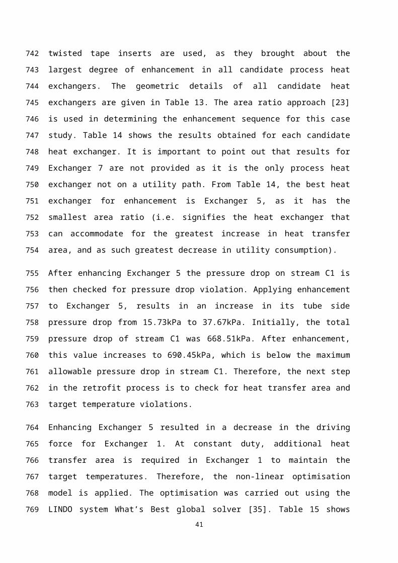
[31] Filonenko, G.K. (1954). Hydraulic resistance in pipes, Teploergetica, 1(4),
40-44.
[32] Elsiedig, A. (2011). Heat Exchanger Network Retrofit Using Shell-Side Heat
Transfer Enhancement. University of Manchester: Manchester.
[33] Zhang, J. F., Li, B., Huang, W. J., Lei, Y. G., He, Y. L., and Tao, W. Q.
(2009). Experimental performance comparison of shell-side heat transfer for
shell-and-tube heat exchangers with middle-overlapped helical baffles and
segmental baffles. Chemical Engineering Science, 64(8), 1643-1653.
[34] Nie, X., and Zhu, X. (1999). Heat exchanger network retrofit considering
pressure drop and heat transfer enhancement. AIChE journal, 45(6), 1239-1254.
[35] LINDO Systems Inc. (2013). What’s Best! 12.0 User’s Manual, LINDO
Systems, Chicago, IL.
41
692
693
694
695
696
697
698
699
700
701
702
703
704