Pressure and Temperature based Adaptive Observer of Air ...annastef/FuelCellPdf/scheme2forJNACfin.pdf · In this paper we design an adaptive air charge estimator for turbocharged

Stefanopoulou et al. - Pressure and Temperature based Adaptive Observer of TC Diesel Air Charge 1

Pressure and Temperature based Adaptive Observer of Air Charge for

Turbocharged Diesel Engines∗

A. G. Stefanopoulou1†, O. F. Storset2, R. Smith3

1University of Michigan, Ann Arbor

2,3University of California Santa Barbara

September 26, 2003

Abstract

In this paper we design an adaptive air charge estimator for turbocharged diesel engines using intake manifold

pressure, temperature and engine speed measurements. This adaptive observer scheme does not depend on

mass air flow sensors and can be applied to diesel engines with no exhaust gas recirculation (EGR). The

performance of the adaptive scheme is shown in simulations to be comparable to conventional air charge

estimation schemes if perfect temperature measurements are available. The designed scheme cannot estimate

fast transients and its performance deteriorates with temperature sensor lags. Despite all these difficulties,

this paper demonstrates that (i) the proposed scheme has better robustness to modelling errors because it

provides a closed loop observer design, and (ii) robust air charge estimation is achievable even without air

flow sensors if good (fast) temperature sensors become available. Finally, we provide a rigorous proof and

present the implementation challenges as well as the limiting factors of this adaptation scheme and point to

hardware and temperature sensor requirements.

Keywords: Estimation, Adaptive, Nonlinear, Engine, Sensors, Automotive, Emissions

1 Introduction

Air charge estimation is an integral part of modern automotive controllers and a critical algorithm for low

emission vehicles. In gasoline throttled port fuel injection engines air charge estimation is used to schedule the∗Support for Stefanopoulou and Storset is provided by the National Science Foundation under contract NSF-ECS-0049025 and

Ford Motor Company through a 2001 University Research Project; Smith is supported by the National Science Foundation under

contract NSF-ECS-9978562.†Corresponding author: Mechanical Engineering, University of Michigan, G058 WE Lay Auto Lab, 1231 Beal Ave, Ann Arbor,

MI 48109-2121, [email protected], TEL: +1 (734) 615-8461, FAX: +1 (734) 764-4256


fuel injection command that will result in a cylinder mixture with stoichiometric air-to-fuel ratio. The air-to-fuel

ratio regulation to the stoichiometric fuel value is a stringent requirement that ensures high conversion of the CO,

HC, and NOx feedgas pollutants to less harmful tailpipe emissions through the Three-Way-Catalytic (TWC)

Converter [1]. The fuel scheduling is typically controlled via a combination of a measured AFR (feedback) signal

and an estimated cylinder air charge (feedforward) signal. Seminal contributions can be reviewed in [2, 3, 4, 5]

and the references therein.

Air charge estimation is used in diesel engines to limit the fuel flow command and avoid low AFR. Low AFR

is undesirable because it results in visible smoke and excessive particulate matter. Turbocharged diesel engines

typically operate with very lean mixtures (AFR>35) thus the fuel is scheduled to meet the driver torque demand

and road load. During fast accelerations or sudden load changes the scheduled fuel flow can cause rich AFR

excursions (AFR<AFRsl=25) and consequently visible smoke generation. The rich AFR excursions last until

the air flow adjusts to a new higher value due to the increase of the exhaust gas energy, and consequent increase

in turbocharger speed and compressor flow [6]. This transient excursion can be avoided if an accurate air charge

estimator is used to trigger an upper limit to the fuel flow that keeps the actual AFR above the smoke limit [7].

The difficulty is mostly during transients and requires characterization of the engine breathing dynamics [8]

to analyze and develop real-time algorithms [9]. Most of the estimation and control algorithms are similar to the

ones developed for throttled gasoline engines taking only into account the differences due to the turbocharger and

intercooler dynamics. The air charge estimation is based again on a static volumetric efficiency map that depends

on intake manifold (boost) pressure and engine speed. During transient fueling changes,however, there are very

large deviations of the instantaneous ratio between the exhaust and intake manifold pressure from their steady-

state values. These transient deviations have significant effects to the value engine breathing capacity and its air

charge estimation. Characterization of this dynamic breathing behavior requires the additional parameterization

of volumetric efficiency with respect to exhaust manifold pressure [10, 11].

Hence additional sensors are considered. In [12] an exhaust manifold pressure sensor is introduced in addition

to an intake manifold pressure sensor to facilitate the prediction of the transient breathing characteristics. The

complexity introduced by the varying intake manifold temperature is addressed in [13] and the authors indicate

the benefits of fast temperature measurement. Additional measurements such as a Universal (linear) Exhaust Gas

Oxygen (EGO) sensor for AFR feedback in [14] and closed loop air charge estimation in [15] are also investigated.

Another important collection of work on air charge estimation is proposing the use of adaptive observers for

on-line estimation of the engine breathing characteristics. This approach is especially desirable due to the reduced

engine mapping requirements and thus easy vehicle calibration and low development cost [16]. It is also necessary

during significant aging and parameter variations [15]. Moreover, it has been proposed in order to account for

the engine dynamic behavior during fast transients after appropriate parameterization [17, 18, 19]. All the above

efforts depend on traditional sensing scheme of speed, intake manifold pressure, and inlet air flow.

In this paper an adaptive air charge estimation scheme is presented that uses intake manifold temperature


sensors instead of the expensive and delicate air flow sensor. The proposed scheme can only work for engines with

no EGR. Indeed, EGR changes the intake mass composition and requires additional measurements. After a few

preliminary notes for the engine model dynamics, the measurements and the system observability are presented

in Section 2, the algorithm is presented in Section 3. The proof delineates the difficulties arising from the slow

temperature sensors and unmodeled sensor dynamics in Section 3.1. A simulation of the estimation scheme

assuming a fast temperature sensor (with 100-200ms time constant) is included in Section 4 to allow comparison

with the traditional estimation schemes. Although such fast thermocouples are not available currently, we believe

that it is important to show what is achievable with this scheme if fast temperature measurements become

available in the future.

2 Preliminaries

In the sequel, (·) denotes a measured variable, or a variable constructed from measurements only, so that x is the

measurement of x. The notation (·) is used for estimated variables and the (·) is used for the error in the estimated

variables. The set of positive real numbers excluding zero is denoted by R+, x denotes ddtx, and Pn(x) is a n-th

order polynomial in x. The operator [Hu](t,N) denotes the filter with the output y = C(N(t))x+D(N(t))u with

x = A(N(t))x + B(N(t))u. For convenience, the dependency on the time varying signal N(t) will be omitted so

that [Hu](t) = [Hu](t,N). Similarly, we will omit the time dependence on signals so that u = u(t), N = N(t),

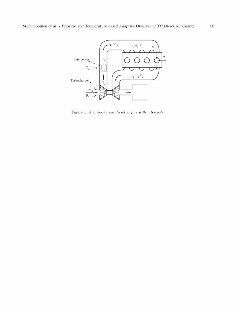
etc. A complete list of all the variables used is in Appendix B. Some of the physical variables are shown in

Figure 1 and we define them in the following text when they are first introduced.

2.1 Model and Estimation Schemes

The engine is approximated as a “continuous flow device” such as a pump. The objective of this paper is to

develop an accurate estimate for the air flow through the engine W1e that is assumed to be constant during a

cycle and is given by

W1e = k21k3Nm1ηv, k3 = Vd

R1120, k1 =

√R1V1

(1)

where R1 is the air gas constant, V1 is the volume of the intake manifold, Vd is the engine total displacement

volume, m1 is the mass in the intake manifold and ηv is the volumetric efficiency [10, 11]:

ηv = ηρ(p2p1

)ηz(N,√

T1), (2)

where ηρ accounts for the pumping losses due to different pressures in the exhaust (p2) and intake (p1) manifold.

The term ηz accounts for the effects of the piston speed which depends on the engine speed (N) and the velocity

of sound in the intake manifold (Mach number) through the temperature (T1).

This model is clearly not valid for short time intervals because it disregards the cylinder-to-cylinder events,

but it has good accuracy on time scales slightly larger than an engine cycle [20, 21, 8]. The energy balance (Eq.


(3)) and mass balance (Eq. (4)) in the intake manifold given adiabatic conditions result in the state equation

for pressure, p1, and mass, m1, respectively. They are related with the intake manifold temperature, T1, through

the ideal gas law (5):

p1 = κk21 (Wc1Ti − W1eT1) (3)

m1 = Wc1 − W1e (4)

T1 = 1k21

p1

m1, (5)

where κ is the ratio of specific heats and Ti the intercooler temperature that depends on compressor and intercooler

efficiencies and is different from T1 during transients. The model described by Eq. (1)-(5) is used after several

simplifications and assumptions in all the existing implementations of air charge estimation. These schemes and

their related measurements are summarized below and serve as basis for comparison.

Modeling the air charge and the cylinder air flow is simplified in throttled engines because the intake manifold

air temperature and the air inlet temperature are considered constant and equal to the ambient temperature

(T1 = Ti = Ta). This eliminates one of the two state equations (3)-(4) and simplifies the intake manifold filling

dynamics. Moreover, the volumetric efficiency can be simplified and represented as a function of the intake

manifold pressure and engine speed, only: ηv = Pv(N, p1). This function can be derived using engine flow

measurements during steady-state conditions.

In the “MAP”-based air charge estimation scheme the key measurement is the intake Manifold Absolute

Pressure (MAP) that provides exact pressure measurements, i.e., p1 = p1. Temperature is measured with

conventional (slow) sensors providing T1. It is almost always true that N = N , and thus, ηv = Pv(N, p1). Open

loop estimation is used to calculate the engine air flow using (1) and (5):

W1e = k3Np1

T1Pv(N, p1) (6)

In addition to modeling errors in Pv that affects both transient and steady-state estimated air charge, this scheme

is prone to temperature variations.

In the “MAF”-based estimation scheme we assume perfect measurement of the mass air flow (MAF) into the

manifold Wc1 = Wc1 (or Wthr = Wthr for throttled engines). This scheme either assumes (i) that the difference

between W1e and Wc1 is negligible and thus uses W1e = Wc1 even during transients, or (ii) utilizes dynamic

compensation for the manifold filling dynamics based on a map of the steady-state air flow Pw(N, p1, T1) as

shown in [22]:

·p1 = κk2

1T1(Wc1 − Pw(N, p1, T1)) (7)

W1e = Pw(N, p1, T1) (= k3Np1

T1Pv(N, p1)). (8)

Errors in Pw(N, p1, T1) and the assumption of constant (or slowly varying) T1 will cause errors during transients.

The two major simplifications that the traditional air charge estimation schemes make are:


(a) Volumetric efficiency and consequently engine air flow do not depend on exhaust manifold pressure (down-

stream pressure).

(b) Intake manifold temperature is constant.

Volumetric efficiency (item (a)) in turbocharged diesel engines is a function of p2. To circumvent the p2 based

parameterization in Eq. (2), we will assume that the volumetric efficiency depends on N and a time varying

parameter θ(t) that needs to be identified so that

ηv(t) = Pρ(N(t))θ(t), (9)

where Pρ(N) > 0 is a polynomial in N that accounts for the pumping rate’s dependency on engine speed. The

variable θ(t) is an unknown time varying coefficient that accounts for all the other phenomena mentioned. Note

that in TC diesel engines we have to assume that θ(t) is a time varying parameter because of the fast variations

of p2p1

. In throttled engines we can assume that θ(t) is an unknown constant or a slow varying parameter as

in [16, 15].

The fact that mass and pressure are independent during transients is usually neglected in conventional esti-

mation schemes where Ti and T1 are assumed equal and constant (item (b)). This variability is represented in

Eq. (3)-(4) and the model we use after the volumetric efficiency parameterization becomes:

p1 = −κk21k3NPρ(N)θp1 + κk2

1Wc1Ti (10)

m1 = −k21k3NPρ(N)θm1 + Wc1. (11)

We use pressure and temperature measurements (Ti and T1) for on-line estimation of θ(t) and then create a

closed loop observer for m1 that is needed for the air flow estimation (Eq. 1). The observability of the system

states with this sensing scheme is presented in Section 2.3.

2.2 Measurements

Sensor selection in engines depends on their cost, reliability and precision. The engine speed N is assumed

measured throughout the sequel, and it is precise so we assume N = N . The flow into the intake manifold,

Wc1, is typically measured with a hot wire anemometer, Wc1, but its performance deteriorates with use even

for expensive devices. This is why we explore its replacement if fast temperature sensors become available.

Intake manifold pressure, p1, can be measured precisely with a large bandwidth at moderate cost relative to

Wc1. However, the engine events cause pressure fluctuations so that p1 = p1 + ∆p1, where ∆p1 represents the

cylinder-to-cylinder flow events and the unmodelled dynamics which are not present in the mean value model.

The term ∆p1 typically has a rectified sinusoidal shape with frequency of the sinusoid equal to 2πN/60 rad/s

appearing as measurement “noise” which might destabilize the identified scheme for the parameter θ(t).


Temperature measurements are typically done with thermocouples which have a time constant varying with

the flow of air. The fastest thermocouples are significantly slower than p1 measurements, so temperature mea-

surements limit the observer bandwidth. However, there is significant development in automotive sensors from

the progression of microelectro-mechanical systems (MEMS) which might result in higher bandwidth automo-

tive temperature sensors in the future. Note here that in experimental configurations, one can use co-axial

thermocouples [23] to obtain fast response metal wall surface temperature measurements.

The temperature of air leaving the intercooler, Ti, can be assumed to be slowly time varying due to the

high efficiency of air-to-air intercoolers and the slowly varying ambient temperature [24]. For better precision a

measurement has to be taken. The cost versus precision considerations are the same as for the T1 measurement.

2.3 Observability based on Temperature Measurements

The issue of observability for a stable plant addresses whether it is possible to create an observer whose state

estimate converges faster to the actual state than the plants dynamics, given perfect knowledge of the plant,

the inputs and the outputs except its present state. In the linear case the famous Kalman rank condition can

be used to check if the plant is observable. However, for a general nonlinear system there is no generic way of

checking observability, and the observer structure is unknown. For completeness we review here some definitions

of nonlinear observability [25].

Observability for the system x = f(x, u) with y = h(x, u) with state x ∈ D, control input u ∈ U and solution

Φ(x(t0), u, t) at time t from the initial condition x(t0), can be defined with the concept of indistinguishable initial

conditions.

Definition 1: Indistinguishable states The initial condition pair (x(t0), x′(t0)), x(t0) �= x′(t0), is said to

be indistinguishable by u if h(Φ(x(t0), u, t), u) = h(Φ(x′(t0), u, t), u) ∀t ≥ t0. If the pair is indistinguishable by all

u; it is said to be indistinguishable.

Definition 2: Observability A nonlinear system is observable if it does not have any indistinguishable pairs

of states.

Notice that observability of a nonlinear system does not exclude the possibility of states indistinguishable by

some inputs. So observability is in general not enough to be able to design a closed loop observer. There have to

be additional constraints on the input. Such an input is called an universal input:

Definition 3: Universal Input An input u ∈ U is universal on [t0, t] if for every pair of distinct states x(t0)

and x′(t0) there exists τ ∈ [t0, t] such that h(Φ(x(t0), u, τ), u) �= h(Φ(x′(t0), u, τ), u). If u is universal for all t > 0

it is just said to be universal.

A non-universal input is called a singular input. If the system is observable and U only contains universal


inputs, it is possible to create an observer whose state converges faster to the actual state than the plants

dynamics. Such a plant is said to be uniformly observable.

Definition 4: Uniformly Observable (UO) A system that is observable and all inputs u are universal is

said to be uniformly observable.

It should be emphasized that even if a system is UO, the observer structure is unknown for a general nonlinear

system. In order to evaluate the observability properties of a system directly from the definition of indistinguish-

able states, it is necessary to have the explicit solution Φ(x(t0), u, t) which is rarely available for nonlinear systems.

It is therefore in general not possible to check observability directly by using the definition of indistinguishable

states.

In our case to estimate W1e we need to produce an estimate of m1 since it cannot be measured directly.

Observability of m1 can then be assessed from p1 and/or T1 measurements assuming correct system equations,

(10)-(11), and perfect knowledge of all the model parameters ηv and Wc1,Ti,N as follows. Equations (10)-(11)

and (5) can be written p1

m1

=

−κk2

1k3N(t)ηv(t)p1 + κk21Wc1Ti

−k21k3N(t)ηv(t)m1 + Wc1

(12)

T1 =1k21

p1

m1(13)

where xT = [p1,m1] is the state and T1 is the output. Equation (12) is a nonlinear system. However, if we

consider u′T = [Wc1Ti,Wc1] any input and N(t) as the known model parameter, the state equation (12) can be

viewed as a linear time varying system p1

m1

=

−κa(t) 0

0 −a(t)

p1

m1

(14)

+

κk2

1 0

0 1

Wc1Ti

Wc1

a(t) = k21k3N(t)ηv(t)

with a nonlinear output equation if y = h(x) = T1 given by (13).

If we denote Φ(x(t0), u, t) the solution to (14) at time t with initial condition x(t0) with input u, the output

becomes

T1(t) = g1(Φ(x(t0), u, t)) (15)

=:1k21

(Φ1(t, t0))κ

p1(t0) + κk21

∫ t

t0(Φ1(t, τ))κ

Wc1Ti(τ)dτ

Φ1(t, t0)m1(t0) +∫ t

t0Φ1(t, τ)Wc1dτ


where the state transition matrix is

Φ(t, τ) = e

−k21k3

t∫τ

N(σ)ηv(σ)dσ

. (16)

Thus, the system (12) is uniformly observable (UO) from (13) because there no states x(t0) �= x′(t0) such that

g1(Φ(x(t0), u, t)) = g1(Φ(x′(t0), u, t)) for all time and all possible inputs. Note that if we consider y = p1 the

output equation (13) does not contain m1, and the system (12) is decoupled, thus observability is lost.

If both p1 and T1 are measured, the system (12)-(13) is obviously observable since it is so in the case when only

T1 is measured. However, it is beneficial to consider this case to see the effects of the additional measurement. In

particular, it is interesting to see that the two measurements together result in a linear time varying system. We

can now disregard the p1 equation in the observability assessment since we measure p1, and there is no coupling

between the states. T1 must now be considered an input, and the system becomes

m1 = −a(t)m1 + Wc1 (17)

p1 = k21T1m1 =: C(u)m1, (18)

which is a linear time varying system. The state transition matrix for this system is (16), and the observability

grammian becomes:

O(t, T, u) =

t+T∫t

ΦT (τ, t)CT (u(τ))C(u(τ))Φ(τ, t)dτ

= k41

t+T∫t

T 21 (τ)e

−2k21k3

τ∫t

N(σ)ηv(σ)dσ

dτ.

Since T1, N and ηv are positive ∀t we have that O(t, T, u) > 0 ∀T > 0, and ∀u = [Wc1, Ti, N, T1] in the

corresponding input space, and we can conclude that m1 is UO from yT = [p1, T1].

Note here that although p1 is measured and thus we can disregard the p1 equation in the observability

assessment, the actual measurement p1 has additional fluctuations that can destabilize the adaptive scheme. Due

to these fluctuations we use a feedback observer for p1 and do not disregard the p1 dynamics from the adaptive

observer.

3 Adaptive Observer Scheme

Since Wc1 is an expensive and often imprecise measurement, it is desirable to develop a scheme that does not rely

on it. Consequently, neither the identification scheme nor the observer can utilize this signal. This is possible

since a parameterization of the plant independent of Wc1 can be derived in any of the coordinates (p1,m1),

(p1, T1) or (m1, T1). By constructing the measurement m1 = 1k21

p1T1

from the ideal gas law (5), it is possible to


realize the equations for the identifier and the observer. For compactness of presentation, this scheme will only

be presented in the coordinates xT := [p1,m1], but by using the same methodology it is possible to derive similar

schemes in the two other coordinates mentioned.

In the observer, Wc1 is replaced with a constant W , and the resulting error is canceled with feedback from

the measurements. The addition of the T1 measurement is essential since the states are not observable from p1

alone. The benefits of the extra measurement are a closed loop observer whose error dynamics converge faster

and are less sensitive to modeling errors than an open loop observer. This identification scheme is sensitive to

errors in Ti since the cancellation of Wc1 in the parameterization makes Ti a factor in the identification error.

Consequently, Ti must be measured, so the total measurements become: p1, T1, Ti and N .

By using the parameterization ηv = Pz(N)θ and adding estimation error injection to equations (10) and (11)

and replacing all signals with their measurements (p1,Ti, m1 = 1k21

p1T1

), and Wc1 = const. = W (any value would

work) the observer becomes:

·p1 = −κk2

1k3NPz(N)θp1 + κk21WTi + gp1(p1 − p1) (19)

·m1 = −k2

1k3NPz(N)θm1 + W + gm1(m1 − m1) (20)

W1e = k21k3NPz(N)θm1 (21)

where, gp1 and gm1 are observer gains to be determined in the design process.

After we multiply (11) with κk21Ti and subtract (10) with the parameterization ηv = Pz(N)θ we derive a

reliable identification scheme that is linear in θ and can guarantee convergence of θ to 0:

κk21Tim1 − p1 = κk2

1k3NPz(N)p1θ − κk41k3NPz(N)m1Tiθ (22)

= −κk21k3NPz(N)

(k21m1Ti − p1

)θ (23)

=: −GpN

(k21m1Ti − p1

)θ (24)

A filter Hf with cutoff frequency linear in N(t) defined as

[Hfu] (t) = xf , with xf = −kωNxf − kωNu (25)

with kω > 0 constant, is used to avoid the pure derivatives in (22). Next, define the signal [φθ] (t):

[Hf (κk2

1Tim1 − p1)]

= (26)

− [HfGpN

(k21m1Ti − p1

)θ]

=: [φθ] (27)

and its implementable versions z(t) and z(t):

z(t) :=[φθ

](t) = − [

HfGpN

(k21m1Ti − p1

)θ](t) (28)

z(t) :=[φθ

](t) = −

[HfGpN

(k21m1Ti − p1

)θ](t). (29)


that are used for the identification error ε(t):

ε(t) := z(t) − z(t) = −[HfGpN

(k21m1Ti − p1

)θ](t) (30)

= φ(t)θ(t) −[Hsφ(τ)

·θ(τ)

](t) (31)

= φ(t)θ(t) − εs (32)

with the regressor, φ(t) = − [HfGpN

(k21m1Ti − p1

)](t). (33)

which is linear in the parameter error θ if we ignore the swapping error εs =[Hsφ(τ)

·θ(τ)

]that arises from

pulling θ out of the filter Hf in (30) using Morse’s swapping lemma [26]. The filter Hs in the swapping lemma

is defined by

[Hsu] (t) := xs, with xs = −kωNxs + u (34)

In Appendix A it is shown that we can obtain an implementable identification error ε:

ε(t) = κk21

[Hf Ti

(d

dτ+ gm1

)(m1 − m1)

]−

[Hf

(d

dτ+ gp1

)(p1 − p1)

](35)

based on measured and estimated variables. The identification error ε is linear in the parameter error θ except

from some terms that depend on the pressure ripples ∆p1 = p1 − p1 and the sensing errors ∆Ti = Ti − Ti,

∆Tm = m1Ti − m1Ti, ∆m1 =·m1 − m1. These terms will cause a bias in the estimate of θ.

The update law is chosen to be the gradient algorithm

·θ =

Γφε ηv = Pz(N)θ ∈ Sη

0 ηv = Pz(N)θ /∈ Sη

,Γ > 0. (36)

where Sη is a bounded set and defined as ηv(t) ∈ Sη := {ηv |0 < ηvMIN ≤ ηv ≤ ηvMAX } ∀t so that θ(t) ∈ Sθ(t) :=

{θ(t)|Pρ(N(t))θ(t) ∈ Sη} ⊂ Sθ ⊂ R+ ∀t.

Theorem: The adaptive air charge estimation scheme summarized as the observer (19)-(21) with the update

law (36) driven by the identification error (35) and the regressor in (33) has the following properties:

[i] Assuming that there are no compressor instabilities, the state xT := [p1,m1] and the input uT := [Ti, T1, N ]

belong in bounded sets, and thus, all the errors θ, p1, m1, W1e are bounded.

[ii] If all the sensing errors and the pressure ripples are zero, and the parameter θ is constant, then the identified

parameter converges to the true constant one (θ → θ) exponentially.

[iii] If we measure the compressor flow accurately in addition to conditions in [ii], then (W1e → W1e) exponen-

tially.

The proof is given in Appendix A.


A simulation of the adaptive estimation compared to the traditional air charge estimation schemes is shown in

Figure 3. It performs similarly to the MAF scheme. The identification error (35) is more sensitive to the ripple

∆p1 and the sensing errors ∆m1 etc. Since the effects caused by the sensing errors increase with the identification

gain Γ, this limits the feasible values for Γ, and in turn the convergence rate of θ. Due to the significant difference

between the temperature and pressure sensor dynamics in this scheme, the higher order dynamics introduced by

the sensors need to be accounted for if the convergence rate of θ is to be acceptable.

This scheme is not vulnerable to possible errors in the Wc1 measurement. In addition, the observer equation

for m1 (20) is closed loop which gives better robustness to modelling errors in the observer. These beneficial

features have been traded with one more measurement, slower convergence time for θ, and most notably that φ

is not always persistently exciting.

The regressor φ is not always persistently exciting (PE). The PE condition fails when k21Tim1− p1 = 0 in some

time interval. If there are no sensor errors and no pressure ripples, the PE condition implies that Ti = 1k21

p1m1

= T1

which is the case at equilibrium, where instability of θ can occur1. This will make θ drift to the boundary of the

projection set Sθ(t). Approximate tracking of the time varying θ(t) cannot be assured when the PE condition

fails. One way to remedy this is to switch the adaption off when the regressor is close to zero and k21Tim1 − p1

is small.

3.1 Unmodelled dynamics introduced by the sensors

The sensors can be assumed to be linear first order systems, so that p1 := Hp1p1, T1 := HT1T1 and Ti := HTiTi.

For example consider the p1 measuring signal p1:

p1 = [Hp1(p1 + ∆p1)] =pp1

s + pp1(p1 + ∆p1) =

1τp1s + 1

(p1 + ∆p1), (37)

which introduces additional dynamics in the identification error ε (second term in the right hand side of Eq. (35)):

Hf

(d

dτ+ gp1

)Hp1 (p1 + p1) (38)

=s + gp1

(τωs + 1)(τp1s + 1)(p1 + ∆p1 − (τp1s + 1)p1)

=s + gp1

(τωs + 1)(τp1s + 1)(p1 + ∆p1 − τp1sp1) (39)

This gives a considerable inverted initial response in θ from·p1.

The slow temperature measurement T1 relative to the p1 measurement creates problems for the m1 approxi-

mation which becomes

m1 =1k21

p1

T1=

[Hp1p] (t)[HT1T1] (t)

. (40)

1See [27] for a treatment of instability phenomena in online parameter identification.


This is very different from a slightly filtered [Hmm1] (t) since the time constant of HT1 is much larger than the

time constant of Hp1. In addition, the sensor dynamics of Ti further worsen the transient behavior of θ and can

even destroy its convergence.

The problem with the m1 approximation can to some extent be removed by filtering with a filter Hc so that

m1 :=1k21

[Hcp1] (t)[HcT1] (t)

=1k21

[HcH

−1p1 p1

](t)[

HcH−1T1 T1

](t)

, (41)

where the bandwidth of Hc is limited by the noise level and the time constant of T1 which is the slowest

measurement. Consequently, the high frequency information in the p1 measurement cannot be utilized if the

temperature measurements are significant slower, and the convergence of θ will be slower. Note also that the

time constant of the temperature measurements is a function of the flow Wc1 which is not measured. This is

a possible obstacle, but if overcome, and in addition the temperature measurements are sufficiently fast, the

response of this scheme is similar to the uncompensated one in Figure 3.

4 Simulation Results

To provide a bit of insight on the practicality of the above analysis we use a mean value model of a turbocharged

2.0 l diesel engine documented in [9] and consequently used for control development in [28] and [29]. The adaptive

air charge estimation is evaluated during fueling level steps (from 5 kg/h to 15 kg/h at time 0.2 s and a negative

step back to 5 kg/h at t=0.7 s). Such a large increase in fuel flow is typically followed by opening the wastegate

or the turbine nozzles in an engine equipped with Variable Geometry Turbocharger (VGT). To match typical

operating engine conditions we also vary the road load. All the input traces are shown in Figure 2.

The volumetric efficiency of the model is

ηv = P3m(N)(1 − 0.003(p′2 − p1)) (42)

where p′2(t) = p2(t − δ(t))

with δ(t) = 60N(t)

12 (one event). Also, P3

m(N) is a third order polynomial representing steady state pumping as a

function of engine speed.

The ηv parameterization for the proposed scheme is

ηv = (P3m(N) + 0.15)θ. (43)

Whereas, the pumping rate for the speed density (“MAP”) scheme in Eq. (8) and mass air flow (“MAF”) scheme

in Eq. (6) is

ηv = Pv(N, p1) = (P3m(N) + 0.15)(1 − 0.003(p2mean − p1)) (44)

Pw(N, p1, T1) = k3Np1

T1Pv(N, p1) (45)


where p2mean is taken to be the average value of p2 in the simulation. In all three cases, ηv has a large constant

deviation of 15% from the one used in the simulation model.

The time constant of Hp1 is 5 ms, and the 2.5% ripple in p1 is represented in the model as

∆p1(t) = (0.127324 −∣∣∣∣sin(

2π

60N(t))

∣∣∣∣)0.0125p1. (46)

The temperature sensor time constant for the MAF schemes is 1.0 s, whereas we assume a time constant of 0.1 s for

the proposed (temperature-based) scheme. Although the adaptive observer has the appropriate filters for dealing

with temperature sensor time constant of 0.1 sec, there are no sensor dynamics modelled when simulating the

proposed scheme.

The estimation parameters for this simulation are: τω = (0.08N)−1, Γ = 0.03, gp1 = 300, gm1 = 1000,

Wc1 = 0.05. The engine air flow estimation results are shown in Figure 3. Although the proposed observer does

not have the bandwidth needed to capture the large initial air excursion, it has a similar W1e estimate with the

traditional “MAF”-based estimator that utilizes a mass air flow sensor and slow temperature measurements. One

should note that the comparison between the proposed and the MAF scheme is unfair due to the differences in the

assumed temperature sensor dynamics. However, the comparison illustrates that robust air charge estimation

is achievable even without air flow sensors if good (fast) temperature sensors are available. This robustness,

reduction in engine mapping, and potential cost elimination from the elimination of the air flow sensor, comes at

the expense of algorithmic challenges and elaborate sensor characterization.

5 Conclusions and Future Work

In this paper we use a temperature measurement instead of mass air flow (MAF) and show that in the case

of zero-EGR the proposed adaptive observer is comparable in performance to the conventional “MAF”-based

air charge estimation. Advances in temperature sensor technology will greatly facilitate adaptive control and

observer design in advanced technology engines because it contains additional information on the dynamics not

easily recovered otherwise.

Fast temperature sensors are considered in addition to flow and pressure sensors in engines with exhaust

gas recirculation. Exhaust gas recirculation gives rise to burnt gas fraction dynamics in the intake and the

exhaust manifold. These dynamics are weakly observable by flow and pressure measurements of intake manifold

variables [13] and require additional sensors such as temperature to enable observability. In-cylinder air estimation

in engines with EGR is much harder and requires more sensors and non-trivial modifications of the proposed

estimation scheme. The air charge estimation for engines with EGR will be addressed in future work.


A Proof of Theorem

As we have indicated in Section 3 the implementable identification error is linear with respect to the parameter

error except from some terms that depend on sensing errors and higher order cylinder-to-cylinder dynamics.

These terms can cause estimation bias or even destabilization, we thus start the proof of [i] by identifying these

terms and then quantifying their effects on the parameter error convergence.

First, let z(t) in (28)

z =[φθ

]= − [

HfGpN

(k21m1Ti − p1

)θ]

(47)

= − [Hf

(GpN

(k21m1Ti − p1

)θ − GpNk2

1(m1Ti − m1Ti)θ + GpN (p1 − p1)θ)]

(48)

= − [HfGpN

(k21m1Ti − p1

)θ] − [

HfGpN

(k21∆Tm + ∆p1

)θ]

(49)

=[Hf

(κk2

1m1Ti − p1

)] − [HfGpN

(k21∆Tm + ∆p1

)θ]

using Eq. (22)-(24). (50)

Similarly, z(t) from (29) can be implemented as

z =[φθ

]= −

[HfGpN

(k21m1Ti − p1

)θ](t) (51)

= −[Hfκk4

1k3NPz(N)m1Tiθ]

+[Hfκk2

1k3NPz(N)p1θ]

(52)

=[Hfκk2

1Ti

( ·m1 − W − gm1(m1 − m1)

)]−

[Hf

( ·p1 − κk2

1TiW − gp1(p1 − p1))]

(53)

=[Hfκk2

1Ti

( ·m1 − gm1(m1 − m1)

)]−

[Hf

( ·p1 − gp1(p1 − p1)

)](54)

where, we used (19)-(20) to derive (53) from (52) above.

Manipulating (50) and (54) and utilizing the sensing error definitions ∆Ti = Ti − Ti, ∆Tm = m1Ti − m1Ti,

∆m1 =·m1 − m1 and the pressure ripples ∆p1 = p1 − p1 we derive the identification error as

ε = z(t) − z

= ε(t) = κk21

[Hf Ti

(d

dτ+ gm1

)(m1 − m1)

]−

[Hf

(d

dτ+ gp1

)(p1 − p1)

](55)

− κk21

[Hf

(Ti∆m1 + ∆Tim1

)]+

[Hf

d

dτ∆p1

]− [

HfGpN

(k21∆Tm + ∆p1

)θ]

If we neglect the terms in the third line of (55), this results in the implementable identification error in (35) or

more specifically:

ε = ε − κk21

[Hf

(Ti∆m1 + ∆Tim1

)]+ [Hdf∆p1] −

[HfGpN

(k21∆Tm + ∆p1

)θ]

= φθ −[Hsφ(τ)

·θ(τ)

]− κk2

1

[Hf

(Ti∆m1 + ∆Tim1

)]+ [Hdf∆p1] −

[HfGpN

(k21∆Tm + ∆p1

)θ]

(56)

where we used (31) to explicitly include the regressor φ and the parameter error θ in the implementable identifi-

cation error ε. We also employed the simplified notation of the filter [Hdfu] =[Hf

ddτ u(τ)

]:

[Hdfu] (t) = xdf + kωNu with xdf = −kωNxdf − k2ωN2u. (57)


Using (36) we define the rate of change of the parameter error:·θ = θ − Γφ

(φθ −

[Hsφ(τ)

·θ(τ)

]− [Hdf∆p1] +

[Hf

(κk2

1

(Ti∆m1 + ∆Tim1

)+ GpN

(k21∆Tm + ∆p1

)θ)])

.

(58)

By expanding the filter notation (25),(34), and (57) and combining them into the dynamical state xa we can

derive the following second order system: ·

xa·θ

=

−kωN + Γφ2 Γφ3

−Γφ −Γφ2

xa

θ

(59)

+

kωN kωN(Γφ2 + kωN) −φ

0 −kωNΓφ 1

fse(∆Ti,∆m1,∆Tm)

∆p1

θ

,

where the term that corresponds to all the sensor errors is fse(∆Ti,∆m1,∆Tm) = κk21

(Ti∆m1 + ∆Tim1

)+

k21GpN∆Tmθ. The linear time varying system in (59) that can be expressed as x = A(t)x+B(t)u is exponentially

stable since the eigenvalues of A(t) + AT (t) can satisfy∫ t

t0

λmax(A+AT )(τ)dτ ≤ −λ(t − t0) + µ ∀t > t0. (60)

for some positive constant λ and µ. If we assume bounded sensing errors one also can show that B(t)u(t) is

bounded. We thus conclude that the parameter error θ is bounded.

Due to the estimation error injection in Eq. 19 and 20 the dynamical systems for p1 and m1 are stable and

their input is bounded, thus, the air flow error W1e is bounded.

A.1 Zero Sensing Errors

If the pressure ripples ∆p1 = p1−p1 and the sensing errors ∆Ti = Ti−Ti, ∆Tm = m1Ti−m1Ti, ∆m1 =·m1−m1

are all zero, then the ε = ε and thus the only bias for the parameter error will depend on the swapping error in

Eq. (32).·θ = θ − Γφ

(φθ −

[Hsφ(τ)

·θ(τ)

])(61)

By expanding the filter Hs to its state space representation we obtain:·θ = θ − Γφ2θ + Γφxs (62)

xs = −kωNxs + φ·θ = −kωNxs + φ

[θ − Γφ2θ + Γφxs

](63)

and its state space form ·

xs·θ

=

−kωN + Γφ2 −Γφ3

Γφ −Γφ2

xs

θ

+

−φ

1

θ, (64)


which can be expressed as x = Ansx + Bθ and has stable dynamics because the eigenvalues satisfy (60) since

λ(Ans+ATns) = λ(A+AT ). As a result, θ is bounded if θ is bounded. Moreover, θ → 0 if θ = 0 (time invariant

volumetric efficiency and correctly parameterized).

A.2 Measured Compressor Air Flow

If there are no pressure ripples and no sensor errors it is easy to show that

·p1 = −gp1p1 − κk2

1k3NPz(N)p1θ + κk21Ti (Wc1 − W ) (65)

·m1 = −gp1m1 − k2

1k3NPz(N)m1θ + (Wc1 − W ) , (66)

W1e = k1k3NPz(N)(θm1 + θm1

). (67)

If the true volumetric efficiency is given by (9), i.e., Pρ = Pz with constant parameter θ, and the compressor

flow is measured (W = Wc1), it is easy to show that p1 → 0, m1 → 0, and W1e → 0.


B Nomenclature

kω filter coefficient

m1 kg mass of gas in the intake manifold

m2 kg mass of gas in the exhaust manifold

N rpm engine speed

p1 kPa pressure in the intake manifold

p2 kPa pressure in the exhaust manifold

pa kPa ambient pressure

R1 kJ/(kg K) gas constant for the intake manifold

r - engine compression ratio

T1 K temperature of gas in the intake manifold

T2 K temperature of gas in the exhaust manifold

Ta K ambient temperature

Tc K Temperature of the air leaving the compressor

Ti K temperature of the gas leaving the intercooler

V1 m3 volume of the intake manifold

Vd m3 total engine displacement volume

W1e kg/s mass flow into the engine

Wc1 kg/s mass flow from compressor to intake manifold

Wt kg/s throttle mass flow

Wf kg/h engine fueling level

Γ - identification gain for the gradient algorithm see Equation 36

ε and ε identification error and implementable identification error

εs swapping error see Equation 32

ηv - volumetric efficiency of the engine

φ and φ regressor signal and implementable regressor signal


References

[1] Shulman M. A., Hamburg D. R., and Throop M. J. Comparison of measured and predicted three-way catalyst

conversion efficiencies under dynamic air-fuel ratio conditions. SAE Technical Paper 820276, 1982.

[2] Turin R. C. and Geering H. P. On-line identification of air-fuel ratio dynamics in a sequentially injected si engine.

SAE Technical Paper 930857, 1993.

[3] Grizzle JW, Dobbins KL, and Cook JA. Individual cylinder air-fuel rato control with a single EGO sensor. IEEE

Transactions on Vehicular Technology, 40(1), 1991.

[4] Mooncheol W, Choi SB, and Hedrick JK. Air-to-fuel ratio control of spark ignition engines using gaussian network

sliding control. IEEE Transactions on Control Systems Technology, 6(5):678–87, 1998.

[5] Powell J. D., Fekete N. P., and Chang C.-F. Observer-based air fuel ratio control. IEEE Control Systems Magazine,

18(5):72–83, 1998.

[6] Fukutani I. Watanabe E., Komotori K., and Miyake K. Throttling of 2-stroke cycle diesel engines at part-load and

idling. SAE Technical Paper 730187, 1973.

[7] Guzzella L. and Amstutz A. Control of diesel engines. IEEE Control Systems Magazine, 18(2):53–71, 1998.

[8] Hendricks E. Mean value modelling of large turbocharged two-stroke diesel engine. SAE Technical Paper 890564,

1989.

[9] Kolmanovsky I.V., Moral P.E., van Nieuwstadt M., and Stefanopoulou A.G. Issues in modelling and control of intake

flow in variable geometry turbocharged engines. Proc. of the 18th IFIP Conf. on System Modelling and Optimization,

1:436–45, July 1998.

[10] Taylor C.F. The Internal-Combustion Engine in Theory and Practice. M.I.T. Press, Cambridge, Massachusetts, 1985.

[11] Yuen W.W. and Servati H. A mathematical engine model including the effect of engine emissions. SAE Technical

Paper 840036, 1984.

[12] Kolmanovsky I.V., Jankovic M., van Nieuwstadt M., and Moraal P.E. Method of estimating mass airflow in tur-

bocharged engines having exhaust gas recirculation. U.S. Patent 6,035,639, 2000.

[13] Diop S., Moral P.E., Kolmanovsky I.V., and van Nieuwstadt M. Intake oxygen concentration estimation for DI diesel

engines. Proc. of the 1999 IEEE International Conference on Control Applications, 1:852–7, 1999.

[14] Amstutz A. and Del Re L.R. EGO sensor based robust output control of EGR in diesel engines. IEEE Transactions

on Control System Technology, 3(1):39–48, 1995.

[15] Kolmanovsky I.V., Sun J., and Druzhinina M. Charge control for direct injection spark ignition diesel engines with

EGR. Proc. of the 2000 American Control Conference, 1:34–8, 2000.

[16] Stotsky A. and Kolmanovsky I.V. Simple unknown input estimation techniques for automotive applications. Proc.

of the 2001 American Control Conference, 5:3312–17, 2001.

[17] Andersson P. and Eriksson L. Air-to-cylinder observer on a turbocharged si-engine with wastegate. SAE Technical

Paper 2001-01-0262, 2001.


[18] Storset OF. Air charge estimation for turbocharged diesel engines. Master’s thesis, University of California Santa

Barbara, 2000.

[19] Storset O.F., Stefanopoulou A.G., and Smith R. Air charge estimation for turbocharged diesel engines. Proc. of the

2000 American Control Conference, 1:28–30, 2000.

[20] Heywood J.B. Internal Combustion Engine Fundamentals. McGraw-Hill, New York, 1988.

[21] Hendricks E. and Sorenson S.C. Mean value modeling of spark ignition engines. SAE Technical Paper 900616, 1990.

[22] Grizzle J.W., Cook J.A., and Milam W.P. Improved cylinder air charge estimation for transient air-to-fuel ratio

control. Proc. of the 1994 American Control Conference, 2:1568–73, 1994.

[23] MEDTHERM Corporation. Coaxial thermocouples with 1 microsecond response. Bulletin 500, March 2002.

[24] Muller M, Hendricks E, and Sorenson SC. Mean value modelling of turbocharged spark ignition engines. SAE

Technical Paper Series 980784, 1998.

[25] Hermann R. and Krener A.J. Nonlinear controllability and observability. IEEE Trans. on Automatic Control, 22:728–

740, 1977.

[26] Morse A.S. Global stability of parameter adaptive control systems. IEEE Transactions on Automatic Control,

25:433–439, 1980.

[27] Ioannou P.A. and Sun J. Robust Adaptive Control. Prentice Hall, New Jersey, 1996.

[28] Stefanopoulou A.G., Kolmanovsky I.V., and Freudenberg J.S. Control of a variable geometry turbocharged diesel

engine for reduced emissions. IEEE Transactions on Control Sytems Technology, 8(4):733–45, 2000.

[29] van Nieuwstadt M., Kolmanovsky I.V., Moraal P.E., Stefanopoulou A.G., and Jankovic M. EGR-VGT Control

Schemes: Experimental comparison for a high-speed diesel engine. IEEE, Control System Magazine, 20(3):63–79,

June 2000.


Intercooler

p2 m2 T2

p1 m1 T1 w1e

wc1

wf

Tc

Ti

pa Ta

Ta

Turbocharger

wc1

Figure 1: A turbocharged diesel engine with intercooler


0 0.1 0.2 0.3 0.4 0.5 0.6 0.7 0.8 0.9 1

5

10

15

Fue

l (kg

/hr)

0 0.1 0.2 0.3 0.4 0.5 0.6 0.7 0.8 0.9 10

0.2

0.4

0.6

0.8

EG

R &

VG

T

0 0.1 0.2 0.3 0.4 0.5 0.6 0.7 0.8 0.9 180

100

120

140

160

180

Load

(N

m)

time (sec)

VGT

EGR

Figure 2: Inputs to the mean-value engine model


0 0.1 0.2 0.3 0.4 0.5 0.6 0.7 0.8 0.9 140

45

50

55

60

65

70

75

80

85

t [s]

MAP-based

Actual

Adaptive Observer

W1e [g/s]

MAF-based

Figure 3: Engine air flow as estimated by the adaptive observer based on engine speed, intake manifold tem-

peratures and pressure. The actual engine air flow as well as the estimated using the traditional MAP- and

MAF-based estimation are shown for comparison.

Documents

Pressure and Temperature based Adaptive Observer of Air ...annastef/FuelCellPdf/scheme2forJNACfin.pdf · In this paper we design an adaptive air charge estimator for turbocharged