Presidential Popularity in a Hybrid Regime:

Russia under Yeltsin and Putin

Abstract

In liberal democracies, the approval ratings of political leaders have been

shown to track citizens‘ perceptions of the state of the economy. By contrast,

in illiberal democracies and competitive autocracies, leaders are often

thought to boost their popularity by exploiting nationalism, exaggerating

external threats, and manipulating the media. Using time series data, I

examine the determinants of presidential approval in Russia since 1991, a

period in which leaders‘ ratings swung between extremes. I find that

Yeltsin‘s and Putin‘s ratings were, in fact, closely linked to public

perceptions of economic performance, which, in turn, reflected objective

economic indicators. Although media manipulation, wars, terrorist attacks,

and other events also mattered, Putin‘s unprecedented popularity and the

decline in Yeltsin‘s are well explained by the contrasting economic

circumstances over which each presided.

Daniel Treisman,

University of California, Los Angeles and NBER*

September 2010

Forthcoming American Journal of Political Science

I thank Yevgenia Albats, Robert Erikson, Lev Freinkman, Tim Frye, Scott Gehlbach, Vladimir

Gimpelson, Patrik Guggenberger, Sergei Guriev, Arnold Harberger, John Huber, Rostislav

Kapelyushnikov, Matthew Lebo, Grigore Pop-Eleches, Brian Richter, Richard Rose, Jim Snyder,

Konstantin Sonin, Stephen Thompson, Jeff Timmons, Josh Tucker, Andrei Yakovlev, Alexei Yudin,

Katya Zhuravskaya and other participants in seminars at the Higher School of Economics, Moscow, and

Columbia University, as well as the editor and three anonymous referees for comments or helpful

suggestions, and the UCLA College of Letters and Science for research support.

Keywords: Presidential approval; hybrid regimes; Russia; economic voting; fractional

cointegration.

* Department of Political Science, UCLA, 4289 Bunche Hall, Los Angeles, CA 90095-1472.

Treisman@polisci.ucla.edu

1

In liberal democracies, the approval ratings of political leaders play an important role in the interaction

between citizens and their governments.1 Like elections—but far more frequently—they communicate to

officials what the public thinks of their performance. Moreover, the messages such polls send have been

shown to make sense. In various Western democracies, leaders‘ ratings tend to rise and fall with the country‘s

economic performance. Respondents appear to hold their leaders responsible and reward them for effective

economic management with approval, much as, when voting retrospectively, they repay competent and honest

incumbents with reelection.

But what role do such ratings play in illiberal democracies and competitive autocracies, where

formally democratic institutions coexist with authoritarian elements? In such states, public opinion is often

viewed as more a product of political manipulation than an input into politics. Even when the polls themselves

are trustworthy, they are thought likely to capture the effects of rulers‘ political theater rather than reasoned

evaluations rooted in material reality. Citizens, fed distorted information by an unfree press and cynical about

the possibilities for participation, are expected to focus on image and personalities rather than to soberly

evaluate performance by studying economic statistics (Ekman 2009). To rekindle their appeal periodically,

incumbents invoke cruder forms of nationalism, exaggerate external threats or terrorist dangers, or even start

military engagements (Mansfield and Snyder 1995).

One country where these issues arise particularly starkly is Russia. Since the first competitive

presidential election there in 1991, presidents‘ ratings have careened wildly. Russia‘s first president, Boris

Yeltsin, started out extremely popular; in September 1991, 81 percent of citizens approved of his performance.

When he left office eight years later, the proportion had dropped to eight percent. His successor, Vladimir

Putin, saw his approval shoot up from 31 percent in August 1999 to 84 percent in January 2000. In his eight

years as president, his rating rose as high as 87 percent and never fell below 60 percent.

To some, these extreme swings reveal the country‘s political immaturity. Journalists attributed both

wars in Chechnya to the desire to boost a Kremlin-backed candidate‘s electoral prospects. Putin‘s appeal has

been explained as the result of an artificially cultivated image as a ―tough‖ leader, the trauma of terrorist

bombings in late 1999, and the Kremlin‘s enhanced control and manipulation of the media. Such

2

interpretations seem to fit the fluidity of the political scene, where parties come and go and politics has often

been seen as primarily the clash of personalities.

But there is another possibility. The volatility of presidents‘ ratings and vote shares might merely

mirror volatility in the economy. Russians might be responding to perceived conditions as logically as do their

Western counterparts. Swings in incumbents‘ approval might reflect not Kremlin manipulation or the

capriciousness of voters but their admittedly crude attempts, in an environment of uncertainty and

unresponsive government, to hold their leaders to account.

Although there are many conjectures about what causes change over time in the popularity of Russian

presidents, few have attempted to confront these systematically with evidence.2 I use statistical techniques and

time series survey data to do so. I look first at what polls reveal directly about the determinants of presidential

popularity. Then, with error correction regression models, I test which factors help predict the trajectories of

presidents‘ ratings.

Understanding what affects the popularity of Russian presidents is important for several reasons. Not

least, it matters for Russian politics. If building support for an incumbent requires only projecting a certain

image, it makes sense for Kremlin operatives to monopolize the mass media. If fighting Chechen terrorists

boosted Putin‘s appeal, such threats are likely to be dramatized as elections approach. However, if the key

element was economic recovery, implications are more benign: leaders will need to master the art of economic

management.

Although Russia is unique in certain ways, the results suggest hypotheses and modes of analysis

relevant to other hybrid regimes. Debates continue over the influence of economics and charismatic populism

over voting and presidential approval in Latin America (Dominguez and McCann 1996, Weyland 2003). Does

Hugo Chavez‘s appeal in Venezuela rest on ideological support for his ―Bolivarian Revolution‖ or on oil-

fueled prosperity? Did Fujimori‘s support in Peru owe more to economic conditions or his counterinsurgency

efforts (Arce 2003)? Scholars have also pondered what shapes presidential popularity in the young

democracies of Asia, exploring, for instance, whether the dips in Indonesian President Yudhono‘s rating in

3

2008 were caused by falling oil prices or the image of the president as weak and indecisive (Mietzner 2009,

p.147).

To preview the results, I find that Russians resemble voters in developed democracies in how they

judge their leaders. Their evaluations closely follow economic conditions. Perceptions of the state of the

Russian economy and of families‘ own finances do a good job of predicting both the decline in Yeltsin‘s

rating, and the surge and plateau in Putin‘s. Although leaders have tried to manipulate perceptions, the

statistical evidence suggests such efforts have had limited effects. At times—notably during certain election

campaigns—Russians‘ views of the economy were rosier than warranted. But in general perceptions were well

predicted by objective economic indicators.

In this paper, I study what determines change in the average popularity of Russian presidents over

time. Other papers, using cross-sectional survey data, have explored what types of individuals supported

Yeltsin or Putin at given moments. Such studies, like this one, tend to find that economic factors were

important (Duch 1995; Miller, Reisinger, and Hesli 1996; Hesli and Bashkirova 2001; Rose, Mishler and

Munro 2004; Rose 2007b; Colton and Hale 2008; White and Mcallister 2008). While this might seem

reassuring, it is important to remember how cross-sectional and time series analyses differ. They do not, as

sometimes thought, generate potentially competing evidence on the same question. Rather, they address

different questions. Cross-sectional analyses show what categories of citizens favored the incumbent at a

particular time. They reveal little about changes in aggregate support. For that, we need time series or panel

data. Of course, time series regressions are unable to assess the importance of characteristics that vary across

individuals but not over time.3

The only time series study of Russian presidential approval of which I am aware is Mishler and

Willerton (2003), which examined data up to 2000, and so was not able to draw strong comparisons between

the Yeltsin and Putin periods. I extend their analysis, and, using the more extensive data now available, draw

somewhat different conclusions.

4

Data on presidential approval

The main data I analyze are from a regular, face-to-face survey conducted by the Russian Center for Public

Opinion Research (VCIOM) until 2003, and then by its successor, the Levada Center. VCIOM, founded in

1988, was directed from 1992 by Yuri Levada, a sociologist who had been fired from Moscow State

University in 1969 for ―ideological mistakes in his lectures.‖ VCIOM earned a reputation as the most

professional and politically independent of Russia‘s half dozen leading polling organizations. This

independence is thought to have prompted a state takeover in 2003, in which Levada was fired. The center‘s

researchers set up the private Levada Center, which continued the polls.

The surveys are of a nationally representative sample of voting-age citizens, who are interviewed in

their homes. I focus on two questions. First, the pollsters ask: ―On the whole do you approve or disapprove of

the performance of [the president‘s name]?‖ This question, similar to one on the US Gallup poll, was included

monthly from late 1996.4 I use it to examine approval of President Putin, first elected in March 2000. Since

this question was asked only occasionally before September 1996, I use another to study Yeltsin‘s popularity.

This one, included every second month from early 1994, asked: ―What evaluation from 1 (lowest) to 10

(highest) would you give the President of Russia Boris Yeltsin?‖5 I analyze the average evaluation.

6 When

both measures are available, the two are highly correlated, in levels (at r = .98) and in two-month differences (r

= .91).

Figure 1 shows the data. On the left, Yeltsin bumps his way down from a December 1990 peak to a

low of 6 percent in early 2009. On the right, Putin glides along, consistently above 60 percent. No American

president has equaled Putin‘s record since regular polling began in the 1930s. Eisenhower came closest, but

even his rating fell at times into the 40s. No British prime minister has come close since the first MORI poll in

1979.7 Nor have post-war US presidents plumbed the depths to which Yeltsin sank—the lowest was Harry

Truman‘s 22 percent in February 1952.

A natural first question, then, is whether the results are believable. Might Putin‘s ratings have been

concocted to please the Kremlin or reflect insincere replies of intimidated respondents? There are reasons to

5

doubt this. First, it is hard to believe VCIOM was slanting results to please Putin given its leader‘s semi-

dissident past and the state‘s takeover to punish it for insufficient loyalty. Various Western pollsters (such as

World Public Opinion and the New Russia Barometer) have worked with the Levada group and found it highly

professional. The dynamics in VCIOM/Levada polls match those in surveys by other organizations. For

instance, in 2006-7 the Levada 10-point rating correlates at r = .93 with the share that said in polls of the Fond

Obshchestvennogo Mnenia that they ―trusted‖ Putin.

Second, it seems unlikely many respondents were intimidated given their critical responses on other

questions. Asked in 2004 whether there was more or less corruption and abuse of power in the highest state

organs than a year before, 30 percent said ―more,‖ 45 percent said ―the same amount,‖ and only 13 percent

said ―less.‖8 Respondents were not shy to give Yeltsin a 6 percent approval rating and Putin just 31 percent in

1999. Even as Russians swooned over Putin, his governments never won the approval of more than 46 percent,

and large majorities opposed some of his policies, including—after the initial period—the military occupation

of Chechnya.9

Another concern is that, by limiting respondents to a 10 point scale, the surveys might be censoring

the data. In the web appendix, I show the distributions of responses around Yeltsin‘s highest and lowest points.

While the distribution is reasonably symmetric for Yeltsin‘s peak, respondents did cluster at the bottom in

1999. If the scale was censoring some respondents, the effect of economic decline under Yeltsin may actually

have been greater than that estimated here.

Possible explanations

What might explain the path of approval in Figure 1? In other countries, the public often rallies behind leaders

at the start of wars (Mueller 1973). Both wars in the southern republic of Chechnya began in the run-up to

presidential elections. In November 1994, Yeltsin‘s aide Oleg Lobov reportedly said that a ―small, victorious

war‖ would ―raise the president‘s ratings.‖10

Putin‘s surge occurred as he sent troops to the republic for a

second time and promised to crush the terrorists who had bombed four apartment buildings. ―People believed

6

that he, personally, could protect them,‖ Yeltsin wrote in his memoirs. ―That‘s what explains his surge in

popularity‖ (Yeltsin 2000, p.338).

Surveys suggest the public viewed the two wars quite differently. Yeltsin‘s use of force in December

1994 was widely condemned; the next month, two thirds of respondents opposed it (Jeffries 2002, p.372). By

summer, 71 percent disapproved of Yeltsin‘s approach to Chechnya. However, opinion soon soured on the

compromise of 1996, under which terrorists regularly crossed the border to take hostages for ransom. In

October 1999, 74 percent favored a major military operation against illegal armed groups in Chechnya.11

Support, however, proved fickle. By July 2000, about two thirds of Russians thought Putin‘s attempts

to rout the insurgents mostly or completely unsuccessful, and the share remained above 60 percent until 2006.

By November 2000, more Russians favored starting peace negotiations than continuing the military operation.

By early 2001, less than one in ten respondents said they were attracted to Putin by his Chechnya policy. If

Putin‘s hard line on Chechnya helped him early on, this does not seem to have been the case later. To capture

attitudes towards Putin‘s Chechnya policy, I use a variable that measures the percentage of respondents who

favored ―continuing the military operation‖ in Chechnya rather than ―negotiating with the ‗fighters‘.‖12

Second, some saw the main reason for Putin‘s popularity and Yeltsin‘s dwindling appeal in their

divergent personal styles. Yeltsin—ailing, gaffe-prone, at times visibly inebriated—could hardly have seemed

more different from the disciplined, energetic, sober Putin, a former spy and judo black belt. Polls confirm that

Russians were attracted by Putin‘s image of youthful vigor and put off by Yeltsin‘s physical decline. Asked

what qualities attracted them to Putin, from 30 to 47 percent of respondents chose ―he is an energetic, decisive,

strong-willed person.‖ Only 9 percent said this of Yeltsin in January 2000. Even in 1996, the third most

frequent thing respondents disliked about Yeltsin was that he was ―a sick, weak person.‖13

But did the presidents‘ images explain their varying support? Unfortunately, regular data on this were

not available; respondents were asked only occasionally about Putin‘s attractions. Governing style is also

manifested in particular incidents. One episode thought to have harmed Putin‘s image was his reaction when

the Kursk nuclear submarine sank in 2000. While the Navy brass dithered, ignoring Western offers of help, the

news showed Putin jet-skiing on the Black Sea. Yeltsin‘s frequent hospital stays cannot have improved his

7

image (Mishler and Willerton 2003). His drinking problem was made vivid in August 1994, when television

showed him jerkily conducting a police band in Berlin.

Putin promised from the start to restore ―order‖ after the turbulent 1990s, to fight crime and

corruption and reimpose control over wayward local officials. A former KGB officer, he seemed to

have the appropriate experience and connections. Could this explain his popularity? In surveys, many Russians

say they favor strong leaders and are willing to sacrifice some rights in return for order.14

However, advocates

of a ―strong hand‖ and other antidemocratic norms turn out to be less likely to support Putin than to back

Communist leader Gennady Zyuganov or the ultranationalist Vladimir Zhirinovsky. In fact, Whitefield (2005)

found it was democracy supporters that favored Putin.15

Moreover, many Russians were skeptical of Putin‘s claims. Periodically, VCIOM/Levada polls asked

how successful Putin had been at imposing order. On average 47 percent thought he had been at least partly

successful; 49 percent thought he had been unsuccessful.16

There was no clear trend. On more specific

questions, reports of deterioration predominated. Each year after 2000, at least 25 percent more thought

citizens‘ personal security had worsened than thought it had improved; at least 15 percent more saw decline in

law enforcement than saw progress.17

Early on, 29 percent liked Putin because he ―could impose order in the

country.‖ By October 2006 the share had fallen to 13 percent.18

Following Mishler and Willerton (2003), I created a measure of Russians‘ political mood from the

question: ―Overall, how would you assess the political situation in Russia?‖ I subtracted the proportion

choosing ―critical, explosive,‖ or ―tense‖ from that saying ―calm‖ or ―favorable.‖ To test whether attacking the

oligarchs and exploiting nostalgia won Putin support, I created dummies for the months after the arrest of the

oligarch Mikhail Khodorkovsky and after Putin restored the Soviet music to the national anthem. A large

plurality—46 percent in a VCIOM poll—favored the Soviet version.19

Respondents credited Putin with ―strengthening Russia‘s international position.‖ Between July 2000

and March 2007, on average 65 percent of respondents said he was quite or very successful at this, compared

to 47 percent who said this of his efforts to ―introduce order in the country.‖ By contrast, many thought Yeltsin

had been too accommodating towards the West, which expanded NATO into Eastern Europe on his watch and

8

then bombed the Serbs over Kosovo. To capture effects of foreign affairs, I included dummies for the Kosovo

bombing, the 9/11 attack, which prompted a pro-American turn on Putin‘s part, and the 2003 US invasion of

Iraq. The Kosovo and Iraq wars were both unpopular in Russia and might have sapped support for presidents

viewed as too cozy with Washington. Under Putin, I also included the share that said he was strengthening

Russia‘s international position minus the share that thought him mostly or completely unsuccessful in this.

To his opponents, Putin‘s ratings simply showed the Kremlin‘s increasing dominance of the press. In

the words of Garry Kasparov: ―You cannot talk about polls and popularity when all of the media are under

state control‖ (Remnick 2007). Under Putin, state companies or loyal businessmen took over the last

independent national television networks. Strong criticism of the president—although not of the government—

disappeared from broadcasts. Based on a 1999 survey, White et al. (2005, p.192) concluded that media bias

helped secure Putin‘s victory: ―The decisive factor in this dramatic reversal of fortunes appeared to be the

media, particularly state television.‖ Measuring change in press freedom was difficult. Lacking a more

sophisticated gauge, I used Freedom House‘s index of press freedom, with the annual value used for each

month of the relevant year. I also created a variable for the month of the state takeover of NTV, the network

previously most critical of the Kremlin.

Finally, economic performance—and, especially, perceptions of it—has been shown to affect approval

of incumbents in the US, France, and Britain (Erikson, MacKuen and Stimson 2002, Lafay 1991, Clarke and

Stewart 1995, Sanders 2000). In Russia, scholars have found economic influences on voting (Colton 2000,

Tucker 2006), and these might also shape presidential popularity. Such effects might be retrospective or

prospective and might focus on respondents‘ own circumstances or their views of conditions nationwide.

Previous studies of post-Soviet countries found evidence of all four types of economic influences. Hesli and

Bashkirova (2001), looking at cross-sectional surveys, found all four effects affected support for Yeltsin.

Mishler and Willerton (2003), focusing on time series data, noted the influence of retrospective evaluations of

the national economy and family finances. Rose et al (2004, p.209) found in a cross-section that views of

current economic performance were the strongest predictor of support for the political regime.

Data were available in the VCIOM/Levada surveys to construct three variables. For retrospective

9

evaluations of the national economy, I use the question: ―How would you assess Russia‘s present economic

situation?‖ For retrospective assessments of personal finances, I use: ―How would you assess the current

material situation of your family.‖ For each of these, I subtracted the shares saying ―very bad‖ or ―bad‖ from

those saying ―very good‖ or ―good,‖ ignoring those who said ―in between‖ or ―don‘t know.‖ For prospective

evaluations of the national economy, I use: ―What do you think awaits Russia in the economy in the coming

several months?‖ I subtracted the percentage anticipating decline from that expecting improvement.20

Unfortunately, no question captured prospective evaluations of personal finances for a comparable period. I

use a dummy for the shock of the August 1998 financial crisis and another for January 2005, when Putin

introduced a reform to replace in-kind benefits such as free bus tickets and drugs for pensioners by cash grants.

This provoked major demonstrations of benefit recipients, who complained that the compensation was

insufficient.

Explaining presidential approval: analysis

Before analyzing the presidential ratings, some statistical issues must be addressed. As is well-known, OLS

regressions on non-stationary data may produce spurious results. I therefore examined whether the approval

data and the time series explanatory variables were stationary, i.e. I(0); had a unit root, i.e. I(1); or were

something in between, i.e. fractionally integrated, I(d) where 0 < d < 1.21

Table 1 shows test statistics for these

series. I use the augmented Dickey-Fuller (ADF) and the Phillips-Perron tests to test the null hypothesis of a

unit root, and the Kwiatkowski et al. (KPSS) and Harris-McCabe-Leybourne (HML) tests to test the null of

stationarity. I treat the two presidencies separately because, examining Figure 1, it seems likely the underlying

process changed between their tenures.22

The tests have weak power and do not always agree. In almost all cases, the HML test—but not the

KPSS test—suggests the series are not stationary.23

In almost all, the ADF and Phillips-Perron tests cannot

exclude the possibility of a unit root.24

Given the likelihood that most or all series are not stationary and the

uncertainty about whether they are exactly I(1), it makes sense to see whether they are fractionally integrated.25

10

I therefore estimated the order of fractional integration, d, for each series in each period, using Robinson‘s

Local Whittle Gaussian ML semi-parametric method (Robinson 1995) (estimates in Table 1).26

I fractionally

differenced each series by its d, estimated for the appropriate period, before including it in regressions.27

I then examined whether the presidents‘ ratings were cointegrated with any of the economic series. If

two variables are cointegrated, a long-run equilibrium relationship exists between them (Box-Steffensmeier

and Tomlinson 2000, p.70). The usual test for cointegration of two I(1) variables is to regress one on the other

and test whether the residuals are I(0), in which case the variables are cointegrated. To test whether two

fractionally integrated series are fractionally cointegrated, one regresses one on the other (both in levels) and

estimates d for the residuals. If the residuals‘ d is less than those for the ―parent‖ series, the variables are

fractionally cointegrated.28

The estimates in Table 1 suggest that Yeltsin‘s rating was fractionally cointegrated

with perceptions of the current economy and/or family finances (the two are highly correlated). Putin‘s

approval may be fractionally cointegrated with economic expectations and support for continuing the military

operation in Chechnya; it may also be cointegrated with the political mood. However, this was highly

correlated with the economic variables and preferred Chechen policy, and tests in the web appendix suggest it

may have been Granger caused by economic expectations.

One revealing way to analyze non-stationary time series is with an error correction model, which

simultaneously estimates the long-run relationship and the short-run dynamics of adjustment. Error correction

models have been used with fractionally integrated series to study various problems (Clarke and Lebo 2003,

Baum and Barkoulas 2006). I use the three-step fractional error correction model of, for instance, Clarke and

Lebo (2003) and Lebo and Cassino (2007). That is, I run regressions of the form:

0 , , 1 1

d d d

t j j t k k t t t

j k

Rating X W ECM (1)

where d indicates that a variable has been fractionally differenced by its estimated value of d; Rating is the

average rating on the 10-point scale (for Yeltsin) or the percentage approving of the president‘s performance

(for Putin); the X‘s, indexed by j, are fractionally integrated explanatory variables; the W‘s, indexed by k, are

stationary explanatory variables; 1

d

tECM is the fractional error correction mechanism (FECM); and ε is a

11

normally distributed stochastic error.29

Where necessary to reduce autocorrelation, I included one lag of the

fractionally differenced dependent variable on the right-hand side (Table 3, columns 1, 2, and 4). To obtain the

FECM, I regressed the president‘s rating on a right-hand variable or variables with which it was thought to be

cointegrated (both in levels), estimated d for the residuals from this regression, fractionally differenced the

residuals by this d, and then lagged the series by one two-month period (see Clarke and Lebo 2003).

The different economic perceptions measures are highly correlated (r = .89, for the current economy

and family finances under Putin), which is not surprising since the same factors are bound to affect all three.

Lacking good instruments, it is easier to assess the aggregate impact of economic perceptions than to be sure

which type matters most. Because of the high correlations, I first present models with each economic

perceptions measure separately and then report a preferred model with more than one, dropping those event

dummies that were not significant at p = .30 (Table 2, column 5; Table 3, column 7). Under Putin, the choice

which economic variables to put in the final model was somewhat arbitrary given the high correlations.

Including family finances together with perceptions of the national economy, the former had an odd negative

coefficient, which I judged to be a spurious result of the correlation between these two variables rather than

evidence that worsening finances boosted Putin‘s popularity. In my view, the data are just not fine-grained

enough to adjudicate between the three types of perceptions. I also include the political mood variable

separately as it is so highly correlated with the economic variables and likely Granger caused by one of them

(see web appendix). I show separate models with the measures of Putin‘s policy performance (on international

affairs, order) since these require shortening the data series. Finally, in Table 2 column 6 and Table 3, column

8, I show the preferred models with the FECM dropped; these are needed for subsequent simulations.

Choosing how to model the influence of discrete events poses a dilemma when the duration of such

effects is unclear. One can arbitrarily assume a path of decay. Or, lacking theoretically-informed priors, one

can try several specifications. The second course reduces the danger of missing the true effect because one has

misspecified the duration, but increases the risk of false positives. In my experience, readers are more

uncomfortable with the latter than with the former. In general, I model each event with a dummy valued 1 in

12

the month of the earliest subsequent survey, and 0 at other times. The impact is thus assumed to decay at the

same gradual rate that the fractional differencing implies.

The one exception is the end of the first Chechen war, which arrived gradually. In March 1996,

Yeltsin decreed a halt to military operations, but this changed little on the ground. In May 1996, he and acting

Chechen President Yandarbiyev signed a ceasefire agreement. But only in late August was the Khasavyurt

Accord signed, actually ending the war. I model this with a dummy valued 1 in May and July, and 0 otherwise

(June and August were not in the bimonthly data). I include simple dummies for the months in which the two

Chechen wars started (since the dependent variables are differenced, dummies for the start and end make more

sense than a dummy for the duration).

As is common in studies of US presidential approval, I control for the time the president had been in

office. Approval of American presidents typically falls, even controlling for other factors. Mueller (1973)

argued that citizens start with unrealistically high expectations and gradually grow disappointed in their

leaders. Under Putin, months in office and the index of press restrictions turn out to be highly correlated (r =

.96); both rose monotonically over time. Therefore, I do not include them in the same regression; months in

office turned out to be more significant in each case.

Table 1 suggested that, under both presidents, more than one variable might be cointegrated with the

president‘s rating. Since it was not obvious a priori which of these—individually or in combination—belonged

in the FECM, I tried several formulations. In Table 2, columns 1 and 5 contain an FECM formed using the

residuals from regressing Yeltsin‘s rating on perceptions of the current economy. In column 2, the FECM used

residuals from Yeltsin‘s rating regressed on perceived family finances. The former proved much more

significant, and also more significant than an FECM for which the cointegrating regression contained both

family finances and the current economy. In Table 3, the FECM uses residuals from regressing Putin‘s

approval on economic expectations. This proved more significant than FECMs that incorporated preferences

on Chechnya policy or the political mood.

What do the results show? Consider first the effects of war and terrorist attacks. Yeltsin‘s Chechen

misadventure appears to have cost him support, although perhaps less than might have been expected. His

13

rating fell at the start of the first war by more than one quarter of a point on the 10 point scale (Table 2,

column 5). It rose as the war ended in 1996, by .31 of a point in both May and July; of course, the estimates

should be viewed as only approximate. Yeltsin lost another quarter point after the 1995 Budyonnovsk terrorist

siege. By contrast, the start of the second war had no clear effect.30

Putin‘s approval rose and fell with support for the use of military force in Chechnya. Since the

latter peaked at 70 percent in March 2000, falling to just 13 percent in December 2007, this suggests the

Chechen situation helped Putin early on, but weighed him down in later years. Indeed, supposing the

coefficients on the fractionally differenced series roughly correspond to those for first differences, Putin lost

about 20-30 points of approval over the course of his presidencies as faith in his military approach dwindled.

Terrorist attacks temporarily revived backing for military force. After the Nordost siege in 2002, support for

the military option leapt from 34 percent in September to 48 percent in November, before falling back to 31

percent in January 2003. This led to a rally behind Putin, whose approval temporarily jumped by six points.

(Nordost had no effect beyond its militarization of the public mood; the dummy is insignificant in Table 3,

where regressions control for support for the military operation.) Beslan led to a smaller jump in support for

military force (from 24 to 31 percent); but Putin‘s approval actually fell that month. The Beslan dummy is

significantly negative, controlling for preferences on Chechnya policy; in other words, support for Putin rose

by less than one would have expected given the militarization of the public mood. One might speculate that in

this case Russians blamed both the terrorists and the authorities for the disastrous outcome.

I lacked good data to assess the influence of presidential style conclusively. But it probably made

some difference. After Yeltsin conducted the band in Berlin, his rating fell by about one quarter point. I found

no evidence, however, that Yeltsin‘s hospitalizations hurt his popularity. Perhaps his ill-health was already too

well-known for this to matter. Putin‘s approval may have fallen after the Kursk sank, but the estimates were

statistically insignificant. Restoring the Soviet music to the national anthem produced a boost of eight or nine

points. It could be that this was the moment Putin ―closed the deal‖ with some former Communist supporters.

Perhaps for the same reason, the arrest of the oligarch Khodorkovsky led to a bounce of about seven points.

Neither respondents‘ assessments of the political situation nor their evaluations of Putin‘s success in

14

international affairs or at establishing ―order‖ significantly affected presidential ratings, although in the latter

cases the limited data might be to blame. After the US invaded Iraq, Putin‘s approval fell several points:

apparently the exercise of American power cast his previous solicitousness of the US after 9/11 in a bad light.

Putin‘s rating also fell after the 9/11 attack. NATO‘s bombing of Kosovo did not have a clear impact on

Yeltsin‘s rating (it was not significant in the final model).

As with US presidents, a time trend remains in Yeltsin‘s and Putin‘s ratings controlling for other

variables. One should interpret the months term along with the intercept; the first was negative for both

presidents, the second positive. This implies that, other things equal, approval tended to rise at first, but then

fall. Such a pattern makes intuitive sense: at first citizens rallied behind a new leader, but over time more and

more grew disillusioned for a variety of reasons not captured by the model. For Yeltsin, the effect turned

negative after about 70 months (mid-1997); for Putin, it remained positive through the end of his second

term.31

The admittedly rough press freedom data do not suggest greater Kremlin control boosted Putin‘s rating.

The NTV takeover had no clear effect. Nor did Freedom House‘s media index; always less significant than

time in office, it was dropped from the regressions. Months in office might, under Putin, be picking up the

trend toward less press freedom. But if so this would suggest that unfree media lowered Putin‘s approval: the

coefficient on months was negative.

These results include a mixture of surprises and confirmations of the conventional wisdom.

Some of the hypothesized factors help account for the spikes in the ratings at various points. But most effects

are small. By contrast, economic perceptions have considerable explanatory power.32

Under Yeltsin, perceptions of the national economy had the strongest impact. The significant FECM in

columns 1 and 5 suggests a long run relationship between rosy views of current conditions and support for the

president. The coefficient‘s value, -.23 in column 5, implies that when a shock knocks the two variables out of

equilibrium, about one quarter of the gap is closed each period. The significant coefficient on fractionally

differenced current economic perceptions suggests these also had a short-term effect. As expected, the 1998

financial crisis depressed Yeltsin‘s popularity. This is not significant if one controls for perceptions of the

current economy, suggesting the crisis affected Yeltsin‘s rating via this pathway. Under Putin, the evidence

15

suggests a long run relationship between economic expectations and presidential approval, with about one

third of any divergence eliminated each period (coefficient of -.32 in column 7). I also found evidence of short

run effects, although the correlations among variables make it hard to say which matters more. Current

economic assessments and expectations are both significant if entered alone (columns 1 and 3), but statistical

significance falls if more than one is included at one time. Again, the strongest short-run effects are of

perceptions of the current economy. As expected, Putin‘s monetization of benefits cost him several percentage

points even after taking into account the impact of the reform on perceptions of family finances.

How much difference did the economy make? One can explore this by simulating the final model

estimated for one president, substituting economic perceptions from the corresponding month in the other‘s

term, while leaving all other variables at their actual levels. The two presidents‘ simulated ratings supposing

each had presided over the other‘s perceived economic conditions are shown in Figure 2, panels A and B.33

This exercise should be taken with a grain of salt. The simulations change somewhat depending on the

specification, and it was not possible to include an FECM.34

Nevertheless, the results are suggestive. It seems

Russians‘ radically different evaluations of their first two presidents were strongly influenced by the very

different economic conditions under which each served. Had Yeltsin presided over Putin‘s economy, he would

apparently have left office extremely popular. Had Putin presided over Yeltsin‘s, his rating would have

plunged early on, recovered a bit, but then sunk again. In January 2008, fewer than 50 percent of Russians

would have approved of his performance.35

The regressions also enable us to explore an intriguing counterfactual about Putin‘s rise, which

is usually seen as inexorably tied to the violent events of late 1999. Suppose there had been no apartment

bombings, no second Chechen war. Would Putin‘s rating have stayed around its starting point of 31 percent?

Of course, we cannot know for sure, but the statistics offer some clues. To see what economic perceptions

alone would predict, I used the estimated effects of just economic perceptions and months in office from Table

1, model 6, and simply extrapolated forward using the actual economic perceptions data under Putin and

restarting months in office. In Figure 3, the dotted line shows the simulated rating of a generic new president

based on just the dramatic economic recovery, supposing Russians started evaluating the new leader in

16

September 1999, right after Putin became prime minister. The dashed line supposes Russians started

evaluating the new incumbent in January 2000, when Putin became acting president.36

The striking implication is that even without a Chechen war or terrorist attacks, economic factors

alone would have prompted a leap in the new president‘s popularity quite similar to that which occurred. In

late 1999, the economy began to revive. Between August 1999 and June 2000, real wages rose by about 20

percent, while wage arrears and unemployment fell. This fueled an unexpected rebirth of economic optimism

that would have boosted support for any new Kremlin incumbent.37

The main difference is that the surge in approval predicted by economic factors comes a little later

than the actual surge. In those months, time was of the essence. Putin would have to run for election in June

2000, or, after Yeltsin resigned early, in March. Were it not for the Chechen war, the Kremlin would have

been best served by the original election schedule. If the public began evaluating Putin in September 1999, by

July 2000 the simulation suggests his rating would have reached 4.5 on the 10-point scale. Supposing instead

that Putin remained tethered to Yeltsin‘s rating until January 2000, by July his would have been 3.7. In 1996,

when Yeltsin won reelection with 54 percent of the valid vote, his rating had been 3.9. Thus, it is very possible

that Putin—or some other new Kremlin candidate—would have won the presidency even without the Chechen

conflict and terrorist bombings.

However, economic factors do not explain why Putin‘s rating actually surged when it did. This might,

indeed, be associated with the Chechen events. Although economic factors would have achieved the same result

a few months later, the traumas of late 1999 apparently sped things up.38

The determinants of economic perceptions

If economic perceptions were important, what caused these perceptions? Did they reflect actual economic

conditions, were they idiosyncratic, or were they manipulated by government propaganda? Russians‘ rosy

view of the economy under Putin might itself result from the Kremlin‘s media control. Or positive economic

perceptions might reflect a general confidence in Putin‘s stewardship.

17

To explore this, I ran fractional error correction models with the fractionally differenced economic

perceptions measures as dependent variables (Table 4). Among explanatory factors, I included six objective

measures of economic conditions—the average real wage, real wage arrears, the average real pension, logged

inflation, unemployment, and the demand for workers (job openings reported to the state employment service).

As might be expected, these were correlated (e.g., r = .87 for the real wage and pension), so besides showing

models that include all six (odd-numbered columns), I present simpler models from which the most

insignificant variables have been dropped (even columns). Given the high correlations, conclusions about

which economic variables were most important have to be tentative. All the economic indicators appeared to

be fractionally integrated, so I fractionally differenced each by the appropriate d (average estimate for

bandwidths 10, 20, and 30; N = 82-4), and included a fractional error correction mechanism. Based on

exploratory analysis, the most appropriate FECM was based on cointegrating regressions including: the real

wage (columns 5-6), the real wage and demand for workers (columns 1-2), and the real wage and

unemployment (columns 3-4).

Besides the official statistics, certain events informed the public about economic conditions. One

might expect gloomier views after the August 1998 financial crisis. Earlier, Russians had been shocked when

on ―Black Tuesday‖ in October 1994 the ruble plunged almost 30 percent, prompting Yeltsin to fire his main

economic ministers. The protests that followed the January 2005 reform of social benefits suggest many

Russians thought this had worsened their financial situation. I also include a dummy for whether the economy

was in its decline or recovery phase, on the theory that expectations tend to overshoot, being too pessimistic in

downturns and too optimistic in recoveries. It is almost a cliché that in business cycles consumers swing

between ―irrational exuberance‖ in the boom and excessive pessimism in the recession; there is some evidence

for this from the US.39

What about political influences? First, causation might run in reverse from presidential approval to

perceptions of economic performance. In the US, overall presidential approval does not appear to affect

consumer sentiment (MacKuen, Erikson, and Stimson 1992), but approval of the president‘s economic

management does (De Boef and Kellstedt 2004). So in estimating the impact of economic indicators on

18

perceptions, one should at least control for presidential ratings; I include the incumbent‘s differenced rating on

the 10-point scale. (My estimate of d was almost exactly 1, so first differencing was appropriate.) Certain

government actions are likely to affect economic perceptions. I included a dummy to see whether Russians

viewed Khodorkovsky‘s arrest as good or bad for the economy (recall that Putin‘s approval jumped). Finally, I

looked for effects of media manipulation. I included a dummy for Putin‘s presidency given the view that

coverage became more favorable under him, and also included the Freedom House index of press freedom.

Media effects are expected to be particularly strong during election campaigns. I included variables valued 1

for the six months before a presidential election and -1for the six months after it.40

Table 4 suggests that Russians‘ views of economic conditions were not just idiosyncratic. Each

perceptions variable is systematically related to objective measures of economic performance. All three appear

to be in long run equilibrium with the average real wage; perceptions of the current economy and family

finances were apparently also in long run equilibrium with, respectively, demand for workers and

unemployment. When real wages rise, economic expectations adjust upward to a new equilibrium, closing

about a quarter of the gap each period (column 6). In the short run, more job vacancies (significant at p = .06)

and perhaps lower wage arrears (p = .09) correlate with a rosier view of the current economy. Short run

increases in pensions (p = .01) and drops in unemployment (p = .04) were associated with cheerier views of

family finances; higher wages may also have helped (p = .08). Rising pensions (p = .01), falling wage arrears

(p = .04), and possibly falling unemployment (p = .13) led to more positive expectations. Inflation was never

significant; its effects might be captured here by real wages and pensions. Attitudes did also overshoot,

accentuating the current trend; even controlling for political factors, views of the current economy and family

finances were more negative in the downslide and positive during the recovery than would be predicted from

just the objective indicators.

As expected, major economic events also triggered reevaluations. The 1998 financial crisis fostered

gloom about the current economy, although oddly it did not influence expectations. Both views of the current

economy and economic expectations worsened after the October 1994 currency crisis. However, these events

did not affect Russians‘ assessments of their own finances, unless such effects were captured by the economic

19

indicators. By contrast, the 2005 monetization of benefits prompted a sharp fall in how well-off many Russians

felt, as well as more pessimistic expectations.

The extent to which objective economic indicators and events can, by themselves, account for the

pattern of economic perceptions can be seen in Figures A2.A and A2.B in the web appendix. In these graphs, I

plot both actual economic perceptions and those predicted using just the economic variables in the regressions

in columns 2 and 4, leaving out political effects. The predictions do not catch all the spikes and dives in

perceptions. But they do an excellent job of capturing the trends.

Politics helps explain the remaining variation. As expected, presidential approval correlated with all

three economic perceptions measures; controlling for it allows greater confidence in the estimated impact of

the economic variables. The coefficients on presidential approval—2.78, 1.44, and 6.91, in columns 2, 4, and

6—suggest the extent of reverse causation. For the current economy and family finances, such effects seem

minor. Of the 84-point range of the current economy variable, presidential popularity could predict about 16

points, and it could predict about eight points of the 77-point range in family finances.41

The possible effect of

presidential approval on economic expectations is somewhat larger—the former could predict up to 39 points

in the 81-point range of the latter.

The dummy for Putin‘s presidency was not significant in columns 1 or 5. It was significant at p = .051

but negative in model 3 for family finances. Of course, it was highly correlated with the economic recovery

variable, which distinguished months after February 1999. Interpreting the two together suggests that

perceived family finances improved a lot in the early recovery months of 1999, but that the effect diminished

after January 2000. Including the economic recovery and Putin dummies separately in the preferred family

finances model (column 4), economic recovery is highly significant but the Putin dummy is not. In short, the

evidence suggests that perceptions were better during the recovery phase, which largely corresponded to

Putin‘s presidencies. But it is not clear that Putin‘s leadership (and media management) had an independent

effect beyond that already captured by the presidential rating. Nor was there evidence that economic

perceptions improved as press freedom decreased, at least as measured by the Freedom House index.

Khodorkovsky‘s arrest led to a boost of some six or seven points in Putin‘s approval (Table 3).

20

Apparently this was in spite of—rather than because of—the economic effect Russians anticipated: after the

arrest, assessments of and expectations for the economy worsened. Russians may have favored the arrest on

grounds of social justice despite fearing adverse economic effects; or perhaps it was different Russians that

applauded Putin‘s action and that anticipated economic reverberations.

Finally, presidential campaigns do seem at times to have influenced perceptions. In 1996 and 2004,

Russians‘ views of the economy and economic expectations improved during the six pre-election months and

fell during the six post-election months by more than expected based on the economic data. Interestingly, the

campaigns brought no improvement in Russians‘ perceptions of their own material situations—these may even

have worsened in 1996—so this might indeed reflect the media‘s influence. There were no significant

campaign effects in 2000, and November 2007 (the only month in the dataset from the 2008 campaign)

actually saw a decline in economic expectations and perceived family finances. Whether the Medvedev

campaign later kicked into gear must await future research.42

Thus, politics does help explain some of the peaks and dips in economic perceptions. Russians‘ greater

approval of Putin than of Yeltsin may have fed back, exacerbating economic pessimism in the late Yeltsin

period and fueling optimism in the early Putin years. Biased media might help explain the surges and falls of

economic optimism around the presidential campaigns of 1996 and 2004. On the other hand, I found no

evidence of systematically greater distortions under Putin than under Yeltsin. Overall, the trends in economic

perceptions were well predicted by just the economic indicators. Perceptions of the economy plummeted under

Yeltsin and soared under Putin not because of effective propaganda but because the underlying economic

variables were doing the same.

Conclusion

In illiberal democracies and semi-authoritarian states, politicians‘ ratings wax and wane, sometimes very

rapidly. Electorates swing between candidates and parties, at times embracing complete unknowns. It is easy

to attribute such fluctuations to an unhealthy brew of rootless and cynical voters, demagogic politicians, and

21

media manipulation. But in some cases the cause may be something else: electoral volatility may mirror

economic volatility—and the efforts of rational voters, against the odds, to hold their leaders to account.

In Russia, Yeltsin‘s plunging popularity and Putin‘s soaring ratings are often linked to their

personalities and public images.43

Some see in Putin‘s ratings an endorsement of his Chechen military

campaign and efforts to rebuild the Russian state (Sil and Chen 2004). Others suppose Russians backed Putin

because they had been brainwashed by a state-controlled media from which criticism of the Kremlin had been

eliminated (Ryzhkov 2004).

Wartime rallies, media effects, and image did play a part at times. Perhaps better data would show

their role to be somewhat greater. However, Russians‘ perceptions of economic conditions have been more

consistently important. Much like citizens in Western democracies, Russians approved of their president when

they saw the economy improving and felt hopeful about its future. Although Kremlin public relations

influenced perceptions, especially in certain electoral campaigns, Russians‘ views of the economy were

closely related to objective economic indicators such as real wages, pensions, and wage arrears.

From this perspective, the fates of Russia‘s first two presidents appear in a new light. Yeltsin‘s

ignominious slide and Putin‘s eight years of adulation seem largely predetermined by the economic conditions

each inherited. (Of course, each influenced the economy on his watch; still, Yeltsin inherited the Soviet system

in mid-collapse, while Putin benefited from a recovery fueled by soaring oil prices.) Simulations suggest a

generic new president would have become extremely popular—judo or no judo—as a result of the boom.

Starting in late 2008 (after the first draft of this paper was written), Russia succumbed to the

international financial crisis. Yet the ratings of Putin (now prime minister) and Medvedev, his successor, did

not drop dramatically. Has the relationship between economics and presidential popularity in Russia changed?

In fact, considered more closely, recent data offer a striking confirmation of the relationships noted here. Two

circumstances are important. First, the Putin government, concerned about social stability, succeeded in

sheltering the public from the full pain of the crisis. Despite an 8 percent drop in GDP per capita in 2009, real

wages fell only 2.8 percent; real disposable incomes actually rose by 1.9 percent because of generous increases

in pensions, which rose by 10.7 percent in real terms that year. Unemployment only increased from 5.7 percent

22

in July 2008 to 8.2 percent in December 2009, less than the US‘s 9.7 percent. Although alarming, the

economic downturn was relatively mild in its effects. Second, the effect of deteriorating economic sentiment

was largely offset by a surge in support for Putin and Medvedev during the war with Georgia in August 2008.

Between July and September 2008, Putin‘s approval leapt from 80.4 to 88.0 percent and Medvedev‘s rose

from 69.4 to 83.0 percent. This was a classic wartime rally behind the flag.

If one subtracts out the 7.6 point jump in Putin‘s approval in September 2008 attributable to the

Georgian war, his rating follows almost exactly the course predicted by the model I previously estimated for

the Putin presidency (column 8 in Table 3) when one enters the actual economic perceptions data for the

Medvedev presidency (see Figure A3 in web appendix). The percentage approving of Putin‘s performance

falls in the simulation from 85 in March 2008 to 69 in November 2009; Putin‘s actual rating minus the

Georgia jump fell from 85 percent to 71 percent. Medvedev‘s rating correlates with Putin‘s at r = .85 in this

period; if we subtract out his even larger jump during the Georgian war, his approval closely parallels the

predicted trajectory.44

Thus, the financial crisis of 2008-9 does appear to have pulled down the leaders‘

popularity, but by a fairly moderate amount since the government took active measures to shelter the

population, and in a way that was largely offset by the wartime rally of support for the Kremlin over the

conflict with Georgia.

The findings of this paper fit with a body of recent work that has been discovering familiar, rational

behavior beneath the irregular surfaces of political life in developing and middle income countries (Drazen

2008). Outside the rich democracies, information is usually asymmetric, uncertainty is endemic, and economic

conditions often fluctuate wildly. In such environments, quite rational behavior can look like impulsiveness and

manipulation. While miscalculations and fraud are certainly common in the hybrid regimes of the developing

and postcommunist worlds, so too, it turns out, is retrospective voting and economics-based evaluations of

incumbents. From Peru to Zambia, ―governments are being held accountable for bad economic policies, at least

to some degree‖ (Lewis-Beck and Stegmaier 2008). The irony is that in such countries economic conditions are

particularly vulnerable to global forces, which complicates the task for citizens—even sophisticated ones—of

separating noise from signals about leaders‘ competence.

23

References

Anderson, Perry. 2007. ―Russia‘s Managed Democracy.‖ London Review of Books, January 25, 2007, 3-12.

Arce, Moisés. 2003. ―Political Violence and Presidential Approval in Peru.”Journal of Politics 65 (May): 572–

583.

Baum, Christopher and John Barkoulas. 2006. ―Dynamics of Intra-EMS Interest Rate Linkages.‖ Journal of

Money, Credit, and Banking 38: 469-82.

Box-Steffensmeier, Janet M. and Renée M. Smith. 1996. ―The Dynamics of Aggregate Partisanship.‖ American

Political Science Review 90: 567-80.

Box-Steffensmeier, Janet M. and Andrew R. Tomlinson. 2000. ―Fractional Integration Methods in Political

Science.‖ Electoral Studies 19: 63-76.

Byers, David, James Davidson, and David Peel. 2000. ―Modeling Political Popularity: an Analysis of

Long-Range Dependence in Opinion Poll Series.‖ Journal of the Royal Statistical Society: A 160: 471-

90.

Cheung, Yin-Wong., and Kon S. Lai. 1993. ―A Fractional Cointegration Analysis of Purchasing Power Parity.‖

Journal of Business and Economic Statistics 11: 103–112.

Clarke, Harold D. and Matthew Lebo. 2003. ―Fractional (Co)integration and Governing Party Support in

Britain.‖ British Journal of Political Science 33: 283-301.

Clarke, Harold and Marianne C. Stewart. 1995. ―Economic Evaluations, Prime Ministerial Approval and

Governing Party Support: Rival Models Reconsidered.‖ British Journal of Political Science 25: 145-70.

Colton, Timothy J. 2000. Transitional Citizens: Voters and What Influences Them in the New Russia.

Cambridge, MA: Harvard University Press.

Colton, Timothy J. 2008. Yeltsin: A Life. New York: Basic Books.

Colton, Timothy J. and Henry E. Hale. 2008. ―The Putin Vote: The Demand Side of Hybrid Regime Politics.‖

George Washington University: unpublished.

De Boef, Suzanna and Paul M. Kellstedt. 2004. ―The Political (and Economic) Origins of Consumer

Confidence.‖ American Journal of Political Science 48: 633-49.

Dominguez, Jorge I., and James A. McCann. 1996. Democratizing Mexico: Public Opinion and Electoral

Choices. Baltimore: Johns Hopkins University Press.

Doukhan, Paul, Georges Oppenheim and Murad S. Taqqu, eds. 2003. Theory and Applications of Long-Range

Dependence: Theory and Applications. Basel: Birkhäuser.

Drazen, Allan. 2008. ―Is There a Different Political Economy for Developing Countries? Issues, Perspectives,

and Methodology.‖ Journal of African Economies 17: 18-71.

24

Duch, Raymond M. 1995. ―Economic Chaos and the Fragility of Democratic Transitions in Former Communist

Regimes.‖ Journal of Politics 37: 121-58.

Dueker, Michael, and Richard Startz. 1998. ―Maximum-Likelihood Estimation of Fractional Cointegration with

an Application to U.S. and Canadian Bond Rates.‖ Review of Economics and Statistics 80 (August): 420–426.

Ekman, Joakim. 2009. ―Political Participation and Regime Stability: A Framework for Analyzing Hybrid

Regimes.‖ International Political Science Review 30: 7–31.

Erikson, Robert S., Michael B. MacKuen, and James A. Stimson. 2002. The Macro Polity. New York:

Cambridge University Press.

Haldrup, Niels and Morten Orregaard Nielsen. 2007. ―Estimation of Fractional Integration in the Presence of

Data Noise.‖ Computational Statistics & Data Analysis 51: 3100-3114.

Hale, Henry. 2009. ―The Myth of Mass Authoritarianism in Russia: Public Opinion Foundations of a Hybrid

Regime.‖ George Washington University: unpublished.

Hesli, Vicki L. and Elena Bashkirova. 2001. ―The Impact of Time and Economic Circumstances on Popular

Evaluations of Russia‘s President.‖ International Political Science Review 22: 379-98.

Jeffries, Ian. 2002. The New Russia: A Handbook. New York: Routledge.

Kramer, Gerald. 1983. ―The Ecological Fallacy Revisited: Aggregate- versus Individual-level Findings on

Economics and Elections, and Sociotropic Voting.‖ American Political Science Review 77: 92-111.

Lafay, Jean-Dominique. 1991. ―Political Dyarchy and Popularity Functions: Lessons from the 1986 French

Experience.‖ In Economics and Politics: The Calculus of Support, eds., Helmut Norpoth, Michael Lewis-Beck,

and Jean-Dominique Lafay. Ann Arbor: University of Michigan Press, 123-39.

Lebo, Matthew J. and Daniel Cassino. 2007. ―The Aggregated Consequences of Motivated Reasoning and the

Dynamics of Partisan Presidential Approval.‖ Political Psychology 28: 719-46.

Lewis-Beck, Michael, and Mary Stegmaier. 2008. ―The Economic Vote in Transitional Democracies.‖ Journal

of Elections, Public Opinion & Parties 18: 303-23.

MacKuen, Michael, B., Robert S. Erikson, and James A. Stimson. 1992. ―Peasants or Bankers? The

American Electorate and the US Economy.‖ American Political Science Review 86: 597-611.

Mansfield, Edward D. and Jack Snyder. 1995. ―Democratization and the Danger of War.‖ International Security

20: 5-38.

Mietzner, Marcus. 2009. ―Indonesia in 2008: Yudhoyono's Struggle for Reelection,‖ Asian Survey 49: 146–155.

Miller, Arthur H., William Reisinger, and Vicki L. Hesli. 1996. ―Understanding Political Change in Post-Soviet

Societies: A Further Commentary on Finifter and Mickiewicz.‖ American Political Science Review 90: 153-66.

Mishler, William and John Willerton. 2003. ―The Dynamics of Presidential Popularity in Post-Communist

Russia: Cultural Imperative versus Neo-Institutional Choice?‖ Journal of Politics 65: 111-141.

25

Morin, Richard, and Nilanthi Samaranayake. 2006. The Putin Popularity Score: Increasingly Reviled in the

West, Russia's Leader Enjoys Broad Support at Home. Washington, DC: Pew Research Center.

Mueller, John. 1973. War, Presidents, and Public Opinion. New York: Wiley.

Remnick, David. 2007. ―Letter from Moscow: The Tsar‘s Opponent.‖ The New Yorker, October 1, 2007.

Robinson, Peter M. 1995. ―Gaussian Semiparametric Estimation of Long Range Dependence.‖ Annals of

Statistics 23: 1630-61.

Rose, Richard. 2007a. ―Going Public with Private Opinions: Are Post-Communist Citizens Afraid to Say What

They Think?‖ Journal of Elections, Public Opinion, and Parties 17: 123-42.

Rose, Richard. 2007b. ―The Impact of President Putin on Popular Support for Russia‘s Regime.‖ Post-Soviet

Affairs 23: 97-117.

Rose, Richard, William Mishler, and Neil Munro. 2004. ―Resigned Acceptance of an Incomplete Democracy:

Russia‘s Political Equilibrium.‖ Post-Soviet Affairs 20: 195-218.

Rzyhkov, Vladimir. 2004. ―The Liberal Debacle.‖ Journal of Democracy 15: 52-8.

Sanders, David. 2000. ―The Real Economy and the Perceived Economy in Popularity Functions: How Much Do

Voters Need to Know? A Study of British Data, 1974-97.‖ Electoral Studies 19: 275-94.

Sil, Rudra and Cheng Chen. 2004. ―State Legitimacy and the (In)significance of Democracy in Post-Communist

Russia.‖ Europe-Asia Studies 56: 347-368.

Tortorice, Daniel L. 2009. ―Unemployment Expectations and the Business Cycle.‖ Brandeis: unpublished.

Tucker, Joshua A. 2006. Regional Economic Voting: Russia, Poland, Hungary, Slovakia and the Czech

Republic, 1990-1999. New York: Cambridge University Press.

Weyland, Kurt. 2003. ―Economic Voting Reconsidered: Crisis and Charisma in the Election of Hugo Chávez.‖

Comparative Political Studies 36 (September): 822-848.

White, Stephen and Ian Mcallister. 2008. ―The Putin Phenomenon.‖ Journal of Communist Studies and

Transition Politics 24: 604-28.

White, Stephen, Sarah Oates, and Ian McAllister. 2005. ―Media Effects and Russian Elections, 1999.‖ British

Journal of Political Science 35: 191-208.

Whitefield, Stephen. 2005. ―Putin‘s Popularity and Its Implications.‖ In Leading Russia: Putin in Perspective,

Essays in Honour of Archie Brown. ed. Alex Pravda. New York: Oxford University Press, 139-160.

Wyman, Matthew. 1997. Public Opinion in Postcommunist Russia. New York: St Martin‘s Press.

Yeltsin, Boris. 2000. Midnight Diaries. New York: Public Affairs.

26

Endnotes

1 The dataset, statistical analysis, and a web appendix for this article are available on the author‘s website at

www.sscnet.ucla.edu/polisci/faculty/treisman/.

2 One exception is Mishler and Willerton (2003).

3 As Kramer (1983) demonstrated: ―There is no reason whatever to expect time-series and cross-sectional

estimates of the same parameters to be similar in magnitude; they need not even be of the same sign.‖ For an

excellent discussion of cross-sectional vs. time series data, see Erikson, MacKuen and Stimson (2002).

4 Gallup asks: ―Do you approve or disapprove of the way that ______ is handling his job as President?‖

5 This question was also used by Mishler and Willerton (2003). In the approval question, sample sizes were

about 1,600; in the 10-point scale questions, the size ranged from 2,100 to about 2,400.

6 I constructed a dataset including just the alternating months in which the question was asked, from early 1994

when the regular series began. In a previous version, I interpolated missing values; however, given the large

amount of interpolation necessary, I prefer here to analyze the bimonthly series. I also use a bimonthly series

for the Putin period since economic explanatory variables were available only every second month.

7 See historical data on the US Gallup poll at www.presidency.ucsb.edu/data/popularity.php and the Ipsos-

MORI polls at http://www.ipsos-mori.com/polls/trends/satisfac.shtml.

8 Results at www.russiavotes.org, Slide 450. Twelve percent picked ―don‘t know.‖

9 Wyman (1997, pp.5-19) reviews the difficulties and common criticisms of polling in Russia, and concludes

that most problems are those faced by survey researchers worldwide. He found ―no evidence specific to Russia

that respondents…. engage in self-censorship.‖ To investigate this, Rose (2007a) asked respondents in 13

postcommunist countries in 2004-5 whether they thought ―people today are afraid to say what they think to

strangers.‖ Among Russians, 25 percent thought people were afraid to some extent—the lowest rate for all 13

countries. Those who thought people afraid to talk—and who were presumably nervous themselves—were

only slightly more likely to favor the current regime, suggesting distortions due to self-censorship are minor.

10 Lobov later denied saying this, but admitted overestimating the odds of a quick success (Colton 2008,

p.290).

27

11

VCIOM, Omnibus poll 1995-4 and Express poll 1999-11, at http://sofist.socpol.ru.

12 The question was not available for the first war. In a previous version I used the percent that said ―war is

continuing‖ in Chechnya rather than ―peace is being established.‖ However, after correcting a data error,

preferences on Chechnya policy were more significant, and also required less interpolation of missing values.

13 VCIOM Express 1996-3, 15-20 February, 1996, 1,584 respondents, at http://sofist.socpol.ru.

14 Does this reveal a cultural predilection for authoritarian rule or just a response to extreme conditions? After

9/11, large majorities of US and British respondents were ready to trade civil liberties for security. In a

YouGov poll of British adults, 70 percent said they were ―willing to see some reduction in our civil liberties in

order to improve security in this country‖ (―Observer Terrorism Poll: Full Results,‖ Observer, September 23,

2001). In a New York Times/CBS poll, 64 percent of US respondents agreed that in wartime ―it was a good

idea for the president to have authority to change rights usually guaranteed by the Constitution‖ (Robin Toner

and Janet Elder, ―A Nation Challenged: Attitudes; Public is Wary but Supportive on Rights Curbs,‖ New York

Times, December 12, 2001). See Hale (2009) for a debunking of the common claim that Russians are

undemocratic.

15 Other polls confirm that Putin is not more popular among supporters of authoritarian government (Morin

and Samaranayake 2006; Rose, Mishler, and Munro 2004).

16 See ―Prezident: otsenki deatelnosti,‖ Levada Center, at http://www.levada.ru/ocenki.html.

17 Levada Center press release, at http://www.levada.ru/press/2007120703.html.

18 I used a measure of the share of respondents who said Putin had been very or quite successful in creating

order in Russia minus the share who thought he had been mostly or completely unsuccessful. As this question

was asked only 14 times, this required shortening the data period and interpolating two thirds of the data.

Similar problems apply to the international affairs variable. Given the need for extensive interpolation, I

include these variables with strong reservations; however, some previous readers thought it important to do so.

19 VCIOM Express poll, 2000-22, 27-30 October, 2000, 1,600 respondents, and Romir Omnibus poll, 2000-11,

1-30 November, 2000, 2,000 respondents. Results available at http://sofist.socpol.ru. In a previous version, in

28

which I interpolated more data, I was able to examine the effect of the constitutional crises of April and

October 1993. Avoiding such interpolation, available data now begin in 1994.

20 These variables were available in a continuous bimonthly series from early 1994, and irregularly before

then.

21 On the analysis of fractionally integrated time series, see, for instance, Box-Steffensmeier and Smith (1996).

22 And analysis using the 10 point scale for both periods (not shown here) confirms that the coefficients on key

variables changed between the two presidencies. Economic perceptions, although still highly significant, had

somewhat smaller coefficients under Putin. It is intuitive to suppose that Russians acclimated psychologically

to the stable growth under Putin and were less sensitive to short run changes than they were to the large,

sustained, irregular economic declines under Yeltsin.

23 The exception is expectations in the Putin period, for which the HML test cannot reject stationarity.

24 The exceptions are economic expectations under Putin, for which the Phillips-Perron, but not the ADF test,

rejects the null of I(1), and possibly also Putin‘s approval (Phillips-Perron test marginally significant).

25 Studies of approval ratings in other countries have also found them to be fractionally integrated (e.g. Byers,

Davidson and Peel (2000), which gives theoretical reasons to expect such data to be fractionally integrated).

26 I used James Davidson‘s Time Series Modeling (TSM) software, v. 4.31. To calculate d, it was necessary to

choose a bandwidth parameter. Unfortunately, as one text puts it: ―In the case of the Gaussian semiparametric

estimator…. [t]here are as yet no satisfactory methods for choosing the bandwidth parameter‖ (Doukhan,

Oppenheim, and Taqqu 2003, p.282). The only recommendation I could find was that of Haldrup and Nielsen

(2007), who suggest choosing relatively low bandwidths, which tend to ―bias estimators less when noise is not

too persistent.‖ I therefore aimed low, calculating d for bandwidths of 5, 10, and 15, and averaging the results.

N was 34 for the Yeltsin series and 50 for the Putin series.

27 Again, I used Davidson‘s TSM software. The fractional differencing formula produces extreme values for

the first numbers in the series (in fact, the first value is the level, not a difference). To prevent such outliers

distorting the results, I dropped the first case from the fractionally differenced series for Putin‘s approval. In

29

the Yeltsin period, I fractionally differenced the series including one interpolated observation from before the

regular series started. I then dropped the corresponding fractionally differenced term.

28 Steffensmeier and Tomlinson (2000) derive this method from Cheung and Lai (1993) and Dueker and Startz

(1998).

29 The three-step method also avoids including non-stationary variables on the right-hand side.

30 That the dependent variable is fractionally differenced makes it harder to interpret the size of the effects. To

get a sense of what difference this makes, I ran versions of the preferred models first-differencing instead of

fractionally differencing the dependent variables. The coefficients were mostly quite similar, at least for the

significant variables, so it is probably safe to assume the effects are roughly as large as those in Tables 2 and 3.

31 To locate the peak, I divide the constant by the coefficient on months in the preferred models.

32 For instance, a model including all the variables in Table 2 except the economic ones has an adjusted R

2 of

.1270. Adding fractionally differenced current economy and family finances along with the FECM raises the

adjusted R2 to .7036. The difference is less dramatic but still notable in the Putin period—adding economic

variables to a model with all non-economic variables raises the adjusted R2 from .4907. to .6630.

33 To simulate Putin with Yeltsin‘s economy, it was necessary to impute values for economic perceptions

under Yeltsin in 1992. To do this, I regressed the economic perceptions variables on inflation and real wages

during months when both were available and used the resulting models to impute backwards.

34 Since one is simulating the dependent variable, one cannot first regress it on economic perceptions to form

the FECM. Instead, I use the models in Table 2, column 6 and Table 3, column 8.

35 In fact, this probably underestimates Putin‘s decline. Not including the FECM, the simulations are unable to

incorporate the long run effect of the fall in economic perceptions under Yeltsin‘s economy.

36 To be clear, no actual data on Putin‘s approval were used to calculate this. I simply used actual economic

perceptions to simulate the incumbent‘s rating, restarting months in office in the relevant month. I therefore

assume nothing about Yeltsin‘s successor except that he took office in September 1999 (dotted line) or January

2000 (dashed line) and that economic perceptions influenced his rating in the same way as under Yeltsin.

30

37

Had Yeltsin been eligible to run for a third term and continued in office, simulations suggest the economic

recovery would also have revived his popularity—but more slowly and less dramatically. As noted, the

accumulated effect of time in office was by that point weighing quite heavily on his rating.

38 As noted, support for military operations fell drastically in subsequent years, which must have pushed down

Putin‘s rating; that it remained high reflects the positive effect of economic stabilization.

39 Tortorice (2009), for instance, finds that American poll respondents are irrationally pessimistic about future

unemployment at the end of a recession and excessively optimistic at the beginning of the downturn. I date the

bottom in Russia by the month in which real wages were lowest, February 1999.

40 For a similar approach, see De Boef and Kellstedt (2004).

41 The range of the presidential rating was 5.6 points. Multiplying this by the coefficients on current economy

and family finances yields 15.6 points for current economy and 8.1 points for family finances.

42 If one assumes each campaign had the same effect, the variable is significant at p = .01 for the current

economy, p = .03 for economic expectations, and not at all for family finances.

43 Anderson (2007) attributes Putin‘s popularity largely to his ―image of firm, where necessary ruthless

authority,‖ and claims to see a link to Russian culture: ―Historically, the brutal imposition of order has been

more often admired than feared in Russia… In what remains in many ways a macho society, toughness—

prowess in judo and drops into criminal slang are part of Putin‘s kit—continues to be valued.‖

44 Since the Levada Center has not published regular data on economic perceptions for this period, I had to

interpolate some observations either linearly or, where possible, regressing the Levada data on answers to

identical questions asked in surveys by VCIOM, the polling organization Levada used to head. (The results of

economic questions on surveys by the two organizations are actually very similar.) Since the Levada Center

stopped asking the question about strategy in Chechnya in December 2007, I assumed support for the military

option remained at its December 2007 level of 13 percent.

31

Table 1. Testing for stationarity and cointegration A. Under Yeltsin (May 1994 - Dec 1999, bimonthly data) Yeltsin rating Current economy Family finances Russia’s ec. future Political situation

ADF test of I(1)

-1.01, p < .90 -1.60, p < .90 -1.72, p < .90 -2.76, p < .10 -1.62, p < .90

Phillips-Perron test of I(1)

-1.22, p < .90 -1.97, p < .90 -2.39, p < .90 -2.56, p < .90 -2.58, p < .90

KPSS test of I(0)

.03, p < 1 .00, p < 1 .02, p < 1 .01, p < 1 .00, p < 1

HML test of I(0)

2.24, p = .01 2.22, p = .01 2.19, p = .01 2.04 p = .02 2.23 p = .01

Estimate of d 0.884 (.17) .909 (.17) 0.977 (.17) 0.505 (.17) 0.553 (.17) Estimate of d for residuals of regression of Yeltsin rating on this variable

0.344 (.17) 0.509 (.17) 0.629 (.17) 1.001 (.17)

B. Under Putin (Jan 2000 - Nov 2007 or Mar 2008, bimonthly data)

Putin approval

Current economy

Family finances

Russia’s ec. future

Military op. in Chechnya

Political situation

ADF test of I(1)

-1.94, p <.90 -.24, p < .95 -1.09, p < .90 -2.41, p < .90 -2.73, p < .10 -.44, p < .90

Phillips-Perron test of I(1)

-2.78 p < .10 -.68, p < .90 -1.80, p < .90 -3.10, p < .05 -2.81, p < .10 -.95, p < .90

KPSS test of I(0)

.00 p < 1 .14, p < 1 .07, p < 1 .15, p < 1 .17, p < 1 .34, p < 1

HML test of I(0)

2.49, p = .01 2.35, p =.01 2.42,p = .01 -.17, p = .57 2.28, p = .01 2.08, p = .02

Estimate of d .646 (.17) 0.725 (.17) 0.470 (.17) 0.635 (.17) 0.604 (.17) 0.634 (.17) Estimate of d for residuals of regression of Putin approval on this variable

.703 (.17) .754 (.17) .492 (.17) .552 (.17)

.592 (.17)

Calculated using James Davidson’s Time Series Modeling software, v. 4.27; p: probability of the test statistic exceeding the computed value under H(0); estimates of d calculated with Robinson’s Local Whittle Gaussian ML semi-parametric method; I present averages of the estimates for bandwidths of 15, 10, and 5 (Yeltsin series have N of 34; those for Putin have N of 50), standard errors in parentheses (averaged across the 3 bandwidths). Yeltsin: 10-point rating; Putin: percent approving of his performance. Standard errors in parentheses.

32

Table 2. Explaining Yeltsin’s popularity, Russia 1994-1999 Dependent variable is fractionally differenced Yeltsin rating on 10 point scale (d = .884)

(1) (2) (3) (4) (5) (6)

d current economy

.031* (.005)

.033* (.004)

.035* (.004)

d family finances

.010 (.012)

.005 (.004)

.007 (.003)

d Russia’s economic future

.011* (.003)

d Political mood

.004 (.010)

d ECM(t-1) -.31*

(.14) -.17 (.13)

-.23* (.09)

Months in office -.006* (.002)

-.004 (.003)

-.004 (.003)

-.004 (.004)

-.006* (.002)

-.005* (.002)

First Chechen war start

-.31* (.08)

-.55* (.09)

-.41* (.09)

-.51* (.18)

-.28* (.06)

-.28* (.06)

First Chechen war end

.35* (.14)

.45* (.11)

.26* (.10)

.35* (.17)

.31* (.12)

.25 (.14)

Budyonnovsk crisis

-.30* (.12)

-.22 (.12)

-.14 (.11)

-.16 (.11)

-.25* (.06)

-.16* (.05)

Start of second Chechen war -.01 (.07)

-.05 (.10)

.05 (.10)

.03 (.14)

Drunk in Berlin

-.19* (.09)

-.19 (.10)

-.17 (.09)

-.17 (.11)

-.23* (.07)

-.27* (.07)

Yeltsin hospitalized .03 (.08)

-.08 (.10)

-.07 (.09)

-.11 (.10)

Kosovo bombing

.06 (.07)

-.01 (.14)

.16* (.07)

.19* (.09)

1998 financial crisis

-.14 (.11)

-.53* (.19)

-.52* (.09)

-.59* (.16)

Constant .42* (.17)

.27 (.22)

.36 (.19)

.31 (.31)

.43* (.13)

.40* (.12)

R

2 .8180 .6171 .6714 .5788 .8250 .7909

LM Autocorrelation test, χ

2 .43, p = .51 .47, p = .49 .00, p = .96 .23, p = .63 .00, p = .97 .03, p = .85

KPSS test of I(0) .05, p < 1 .08, p < 1 .13, p < 1 .13, p < 1 .06, p < 1 .07, p < 1 Durbin Watson statistic 2.00 1.73 1.91 1.73 1.83 1.97 N 33 33 33 33 33 33 * p < .05. OLS with robust standard errors in parentheses. Data are bimonthly, starting in May 1994, when continuous bimonthly economic series

begin, ending in December 1999. d

series fractionally differenced using d estimated in Table 1. ( 1)

dECM t in columns 1 and 5 is the

fractionally differenced residuals from a regression of Yeltsin’s rating on perceptions of the current economy (both in levels), lagged one two-month period; in column 2, the residuals are from a regression of Yeltsin’s rating on perceived family finances. Column 5 shows the preferred model (in bold), from which event variables not significant at p = .30 have been dropped. Column 6 shows a regression identical to that in column 5 except without the ECM.

33

Table 3. Explaining Putin’s popularity, Russia 2000-2008 Dependent variable is fractionally differenced percent approving of Putin’s performance (d = .646)

(1) (2) (3) (4) (5) (6) (7) (8)

d current economy .38*

(.11)

.33*

(.16) .35* (.16)

d family finances -.01

(.23)

d Russia’s ec. future .18*

(.07) .07

(.08) .04 (.10)

d Political mood .10

(.07)

d Successful: International affairs

.19 (.14)

d

Successful: order .11 (.22)

d continue milit. op. in Chechnya

.41* (.16)

.31 (.21)

.45* (.12)

.32 (.21)

.41* (.17)

.40* (.19)

53* (.07)

.56* (.08)

d

ECM(t-1) -.41* (.10)

-.41* (.13)

-.34* (.11)

-.46* (.13)

-.13 (.13)

-.14 (.14)

-.32* (.10)

Months in office -.03 (.02)

-.03 (.02)

-.04 (.02)

-.03 (.02)

-.05 (.03)

-.04 (.03)

-.04* (.02)

-.05* (.02)

Nordost theater siege 1.12

(2.97) 2.07 (3.96)

1.69 (2.45)

3.77 (4.41)

-1.93 (3.19)

.22 (3.43)

Beslan terrorist attack -5.80* (1.97)

-6.85* (2.14)

-6.79* (1.76)

-2.97 (3.96)

-6.25* (2.00)

-7.13* (1.85)

-6.73* (1.17)

-6.38* (1.21)

Sinking of Kursk -1.05

(1.07) -2.89 (1.53)

-1.94 (1.37)

-1.63 (1.63)

-5.05* (2.21)

-2.22 (2.71)

Soviet anthem restored

8.66* (1.16)

8.64* (1.65)

7.95* (1.17)

9.08* (1.45)

10.34* (1.41)

10.04* (1.85)

8.78* (.84)

9.18* (1.20)

Nine eleven -4.79* (1.47)

-1.49 (1.91)

-4.24* (.69)

-2.18 (1.62)

-2.82 (1.98)

-1.85 (1.53)

-6.12* (1.01)

-5.89* (1.18)

Iraq war -3.64*

(.76) -4.94* (1.50)

-4.44* (.80)

-4.60* (.77)

-4.31* (.82)

-5.47* (1.93)

-3.59* (.66)

-3.59* (.75)

Monetization of benefits, Jan 2005

-4.76* (1.00)

-6.32 (4.56)

-4.30* (1.05)

-5.98* (1.02)

-4.26* (1.15)

-4.71* (1.49)

-3.95* (.94)

-3.12* (.84)

Takeover of NTV .72 (1.12)

.16 (1.46)

.02 (1.37)

.33 (1.36)

-2.25 (2.85)

.19 (1.62)

Arrest of Khodorkovsky

6.50* (1.12)

4.85* (1.40)

5.45* (.99)

4.83* (1.22)

5.01* (2.14)

7.10* (2.03)

6.90* (1.08)

8.67* (.89)

L1

d rating .10

(.06) .13 (.08)

.13 (.08)

Constant 5.61* (1.33)

6.10* (1.53)

7.12* (1.39)

5.50* (1.74)

5.82* (1.53)

7.11* (1.78)

6.74* (.95)

6.97* (1.25)

R2 .7707 .6887 .7118 .7054 .6420 .5984 .7540 .6936

LM Autocorrelation test, χ

2

.18, p =.68

.00, p =.96

.35, p =.55

.06, p =.80

.16, p =.69

.15, p = .70

.33, p =.57

.79, p =.38

KPSS test of I(0) .24, p < 1 .24, p < 1 .31, p < 1 .23, p < 1 .14, p < 1 .22, p <1 .29, p < 1 .24, p < 1 Durbin Watson statistic 1.86 1.94 1.81 1.89 2.08 1.87 1.81 2.19 N 47 47 47 47 40 40 47 47

* p < .05. OLS with robust standard errors in parentheses. Data bimonthly, starting in early 2000 and ending in December 2007. d

series

fractionally differenced using d estimated in Table 1. ( 1)d

ECM t is the fractionally differenced residuals from a regression of Putin’s

approval on expected performance of the national economy (both in levels), lagged one two-month period. Preferred model in bold.

34

Table 4. Determinants of economic perceptions

Dependent variable d current economy (d = .947)

d family finances (d = .832)

d Russia’s ec. future (d = .884)

(1) (2) (3) (4) (5) (6) Economic data

d

real wage .007 (.011)

.004 (.011)

.012 (.007)

.007 (.020)

d real wage arrears -.041

(.035) -.040 (.024)

.073 (.057)

-.12* (.05)

-.11* (.05)

d

average real pension .023 (.023)

.051* (.022)

.051* (.019)

.10 (.05)

.094* (.035)

d log inflation 4.24

(3.73) 2.48

(4.23) 3.04

(7.40)

d unemployment -.21

(.98) -2.49

(1.34) -2.82* (1.33)

-2.91 (2.40)

-2.77 (1.83)

d demand for workers .007

(.006) .008

(.004) -.001 (.005)

-.00 (.01)

d ECM(t-1) -.50*

(.08) -.51* (.08)

-.48* (.09)

-.45* (.11)

-.27 (.15)

-.27* (.12)

Recovery phase .97 (1.73)

1.75* (.82)

8.66* (2.27)

3.13* (.89)

1.21 (4.54)

Economic events 1998 financial crisis

-20.16* (4.91)

-18.84* (2.39)

-.61 (6.97)

-2.99 (7.60)

Oct. 1994 financial crisis -6.43* (2.48)

-5.76* (.99)

-1.65 (2.58)

-11.73* (5.39)

-12.48* (1.28)

Monetization of benefits, Jan 2005

-.48 (1.33)

-15.27* (2.01)

-15.05* (1.64)

-5.89 (3.06)

-5.41* (2.05)

Politics Putin presidency dummy .41

(1.71) -4.99

(2.50)

-3.62 (4.69)

President’s rating (10 point scale)

3.08* (1.08)

2.78* (.83)

2.11* (.72)

1.44* (.45)

7.23* (1.71)

6.91* (1.69)

Khodorkovsky arrested

-6.68* (1.45)

-6.14* (1.17)

.45 (1.98)

-6.24* (2.80)

-6.10* (2.15)

Press freedom (high = less free)

.00 (.09)

-.06 (.08)

.10 (.17)

1996 campaign 3.95* (1.38)

4.13* (1.03)

-1.19 (1.38)

-1.70 (.92)

3.57 (2.15)

3.86* (1.93)

2000 campaign -1.30 (2.37)

-1.10 (1.99)

6.16 (7.19)

6.94 (7.15)

2004 campaign 5.37* (1.08)

5.41* (1.02)

-.17 (1.10)

8.53* (1.70)

8.79* (1.54)

2008 campaign -1.75 (1.58)

-3.66* (1.42)

-4.46* (.65)

-5.89* (2.33)

-4.29* (.94)

Constant -.53 (4.84)

-.63 (.67)

.82 (4.50)

-2.31* (.75)

-4.76 (8.75)

.31 (.73)

R

2 .6537 .6255 .6782 .6030 .5129 .5039

LM Autocorrelation test, χ2

(p) .02 (.90) .19 (.67) .03 (.86) .42 (.52) .19 (.66) .20 (.66) KPSS test of I(0) .04, p < 1 .04, p < 1 .04, p < 1 .19, p < 1 .05, p < 1 .10, p < 1 Durbin Watson statistic 2.00 2.05 1.95 2.06 2.08 2.09 N 80 80 80 80 80 80

* p < .05. OLS with robust standard errors in parentheses. Data bimonthly, starting in early 1994, ending in December 2007. d

: series

fractionally differenced using estimated d (average for bandwidths of 30, 20, and 10). ( 1)d

ECM t : fractionally differenced one period lag of

residuals of regression of dependent variable on: a) real wage and demand for workers (columns 1-2); b) real wage and unemployment (columns 3-4); c) real wage (columns 5-6). Even columns show models from which the most insignificant variables have been dropped.

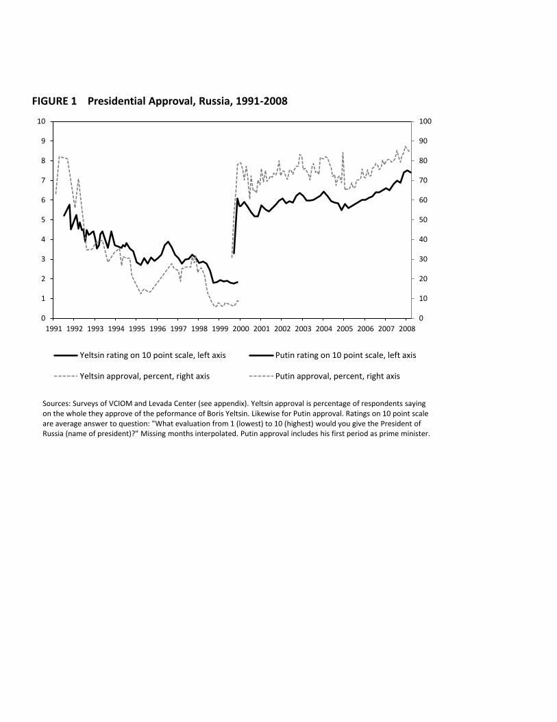
0

10

20

30

40

50

60

70

80

90

100

0

1

2

3

4

5

6

7

8

9

10

1991 1992 1993 1994 1995 1996 1997 1998 1999 2000 2001 2002 2003 2004 2005 2006 2007 2008

FIGURE 1 Presidential Approval, Russia, 1991-2008

Yeltsin rating on 10 point scale, left axis Putin rating on 10 point scale, left axis

Yeltsin approval, percent, right axis Putin approval, percent, right axis

Sources: Surveys of VCIOM and Levada Center (see appendix). Yeltsin approval is percentage of respondents saying on the whole they approve of the peformance of Boris Yeltsin. Likewise for Putin approval. Ratings on 10 point scale are average answer to question: "What evaluation from 1 (lowest) to 10 (highest) would you give the President of Russia (name of president)?" Missing months interpolated. Putin approval includes his first period as prime minister.

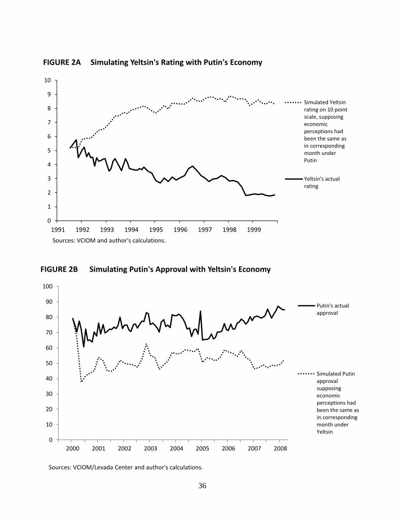
36

0

1

2

3

4

5

6

7

8

9

10

1991 1992 1993 1994 1995 1996 1997 1998 1999

FIGURE 2A Simulating Yeltsin's Rating with Putin's Economy

Simulated Yeltsinrating on 10 pointscale, supposingeconomicperceptions hadbeen the same asin correspondingmonth underPutin

Yeltsin's actualrating

Sources: VCIOM and author's calculations.

0

10

20

30

40

50

60

70

80

90

100

2000 2001 2002 2003 2004 2005 2006 2007 2008

FIGURE 2B Simulating Putin's Approval with Yeltsin's Economy

Putin's actualapproval

Simulated Putinapprovalsupposingeconomicperceptions hadbeen the same asin correspondingmonth underYeltsin

Sources: VCIOM/Levada Center and author's calculations.

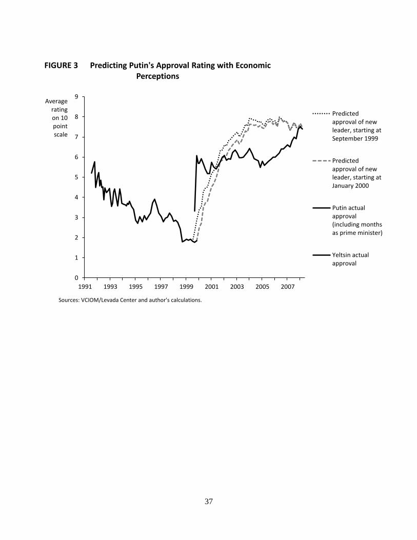
37

0

1

2

3

4

5

6

7

8

9

1991 1993 1995 1997 1999 2001 2003 2005 2007

FIGURE 3 Predicting Putin's Approval Rating with Economic Perceptions

Predictedapproval of newleader, starting atSeptember 1999

Predictedapproval of newleader, starting atJanuary 2000

Putin actualapproval(including monthsas prime minister)

Yeltsin actualapproval

Average rating on 10 point scale

Sources: VCIOM/Levada Center and author's calculations.

38

Web Appendix for ―Presidential popularity in a hybrid regime: Russia under

Yeltsin and Putin‖

Distribution of evaluations of Yeltsin on 10-point scale

Figure A1.a Distribution of evaluations of

Yeltsin's performance, October 1991

0

5

10

15

20

1 2 3 4 5 6 7 8 9 10

Score on 10 point scale

Perc

en

t o

f valid

resp

on

ses

Figure A1b. Distribution of evaluations of

Yeltsin's performance, September 1999

0

10

20

30

40

50

60

70

80

1 2 3 4 5 6 7 8 9 10

Score on 10 point scale

Perc

en

t o

f valid

resp

on

ses

39

Predicting economic perceptions with just objective economic indicators and events

-100

-90

-80

-70

-60

-50

-40

-30

-20

-10

0

1994 1995 1996 1997 1998 1999 2000 2001 2002 2003 2004 2005 2006 2007

FIGURE A2.A Perceptions of the National Economy and their Economic Determinants

Russians'assessmentof thecurrentnationaleconomy

Assessmentof thenationaleconomypredictedfrom justeconomicvariables

Sources: VCIOM, Levada Center, and author's calculations.

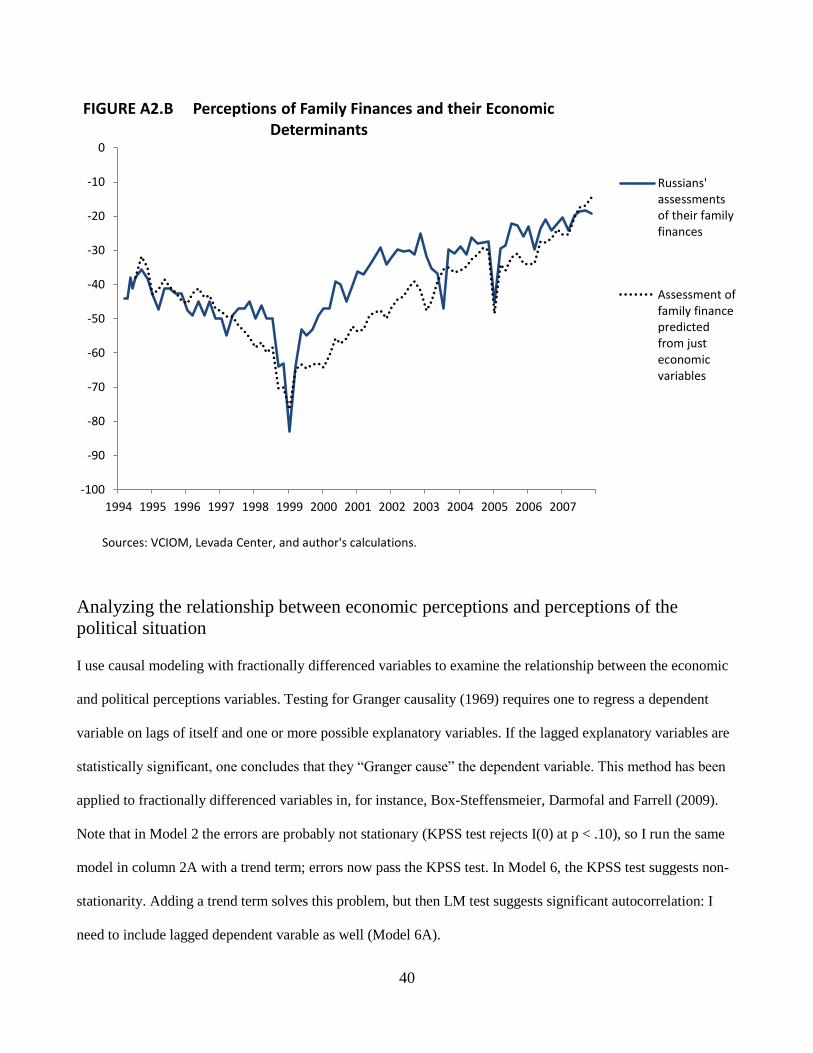
40

Analyzing the relationship between economic perceptions and perceptions of the

political situation I use causal modeling with fractionally differenced variables to examine the relationship between the economic

and political perceptions variables. Testing for Granger causality (1969) requires one to regress a dependent

variable on lags of itself and one or more possible explanatory variables. If the lagged explanatory variables are

statistically significant, one concludes that they ―Granger cause‖ the dependent variable. This method has been

applied to fractionally differenced variables in, for instance, Box-Steffensmeier, Darmofal and Farrell (2009).

Note that in Model 2 the errors are probably not stationary (KPSS test rejects I(0) at p < .10), so I run the same

model in column 2A with a trend term; errors now pass the KPSS test. In Model 6, the KPSS test suggests non-

stationarity. Adding a trend term solves this problem, but then LM test suggests significant autocorrelation: I

need to include lagged dependent varable as well (Model 6A).

-100

-90

-80

-70

-60

-50

-40

-30

-20

-10

0

1994 1995 1996 1997 1998 1999 2000 2001 2002 2003 2004 2005 2006 2007

FIGURE A2.B Perceptions of Family Finances and their Economic Determinants

Russians'assessmentsof their familyfinances

Assessment offamily financepredictedfrom justeconomicvariables

Sources: VCIOM, Levada Center, and author's calculations.

41

Table A1 Economic and political perceptions: causal modeling -------------------------------Yeltsin presidency----------------------------- -------------------------------Putin presidency--------------------------------- 1

d political situation

2 d

political situation

2A d

political situation

3 d

current economy

4 d

Russia’s ec. future

5 d

political situation

6 d

political situation

6A d

political situation

7 d

current economy

8 d

Russia’s ec. future

L1 d

political situation .44* (.11)

.32* (.13)

.10 (.14)

-.03 (.10)

.22 (.22)

-.19 (.13)

-.23 (.14)

-.34* (.16)

.01 (.06)

-.13 (.20)

L1 d

current economy .13 (.24)

.18 (.18)

-.07 (.31)

-.16 (.18)

L1 d

Russia’s ec. future

.25 (.14)

.31* (.15)

.30 (.18)

.06 (.19)

.18 (.20)

.25 (.24)

L2

d dependent var.

.02

(.21) -.10

(.09) .21

(.18) Trend

.26*

(.11) .19

(.10)

Constant -5.33*

(1.19) -5.24* (1.27)

-12.10* (3.02)

-1.16 (1.44)

-.83 (3.19)

5.13* (1.61)

4.96* (1.65)

-5.84 (6.23)

2.50* (.70)

2.07 (1.22)

R2 .3175 .3772 .4668 .0237 .1398 .0423 .0437 .1038 .0223 .1235

Durbin Watson 2.17 1.97 1.79 1.92 1.73 1.97 2.00 1.99 2.00 1.99 LM autocorrelation test, χ

2 1.02,

p = .31 .00 p =.98

.70 p = .40

.15 p = .70

.01 p =.94

.23 p =.63

1.19 p =.28

.27, p = .60

.43 p =.51

1.01 p =.32

KPSS test of I(0) .30 (p < 1)

.37 (p < .1)

.14 (p <1)

.11 (p < 1)

.09 (p < 1)

.33 (p < 1)

.35 (p < .1)

.17 (p < 1)

.21 (p < 1)

.11 (p < 1)

N 33 33 33 33 32 50 50 50 50 50

* p < .05. OLS with robust standard errors in parentheses.d

: series fractionally differenced using d estimated in Table 1; Lk: kth lag of the variable. Lags of the dependent variable were included when necessary to reduce autocorrelation. Trend was included when necessary to render residuals stationary.

42

From the estimates in Table A1 it appears that Russians‘ expectations about future economic

performance Granger caused their evaluations of the political situation during the Yeltsin period (this is

significant at p = .04 in Model 2A). Evidence of causation running from evaluations of the political system to

expectations of future economic performance was less significant (p = .34 in Model 4). There was no clear

evidence that economic perceptions affected political perceptions (or vice versa) during the Putin period,

however.

55

60

65

70

75

80

85

90

95

Mar May July Sep Nov Jan-09 Mar May July Sep Nov

FIGURE A3 Putin's and Medvedev's Ratings in 2008-9, Actual and Predicted with Economic Perceptions

Actual Putin rating

Actual Putin ratingminus the Georgiawar jump

Putin ratingpredicted witheconomicperceptions

Medvedev ratingminus the Georgiawar jump

Percent approving

of leader's

perform-ance

Sources: Levada Center and author's calculations. Predictions formed using Table 3, model 8, with actual economic perceptions for 2008-9; some values in economic series interpolated linearly or using regressions of Levada data on VCIOM data from surveys that asked the same question; percentage supporting military action in Chechnya assumed to have stayed at the December 2007 level (question was no longer asked by Levada Center).

43

Table A2 Variable definitions and data sources Variable Definition Source

____10pt

What evaluation from 1 (lowest) to 10 (highest) would you give the President of Russia, __________? Mar 1994-Nov 1999, bimonthly series, average response.

http://sofist.socpol.ru, http://www.levada.ru/programs.html, Ekonomicheskie i Sotsialnie peremeni: monitoring obshchestvennogo mnenia, various issues, Russiavotes.org

____app

On the whole do you approve or disapprove of the performance of President ____? % saying they approve. Sep 1996-Mar 2008, bimonthly series.

http://www.levada.ru/programs.html, Ekonomicheskie i Sotsialnie peremeni: monitoring obshchestvennogo mnenia, various issues, Russiavotes.org

Putapbacktosep

Percent approving of Putin's performance as President (Jan 2000-Mar 2008) concatenated with percent approving of Putin's performance as PM (Sep -Nov, 1999).

http://www.levada.ru/programs.html, Ekonomicheskie i Sotsialnie peremeni: monitoring obshchestvennogo mnenia, various issues, Russiavotes.org

tenpt average 10pt ratings for Yeltsin and Putin concatenated.

http://sofist.socpol.ru, http://www.levada.ru/programs.html, Ekonomicheskie i Sotsialnie peremeni: monitoring obshchestvennogo mnenia, various issues, Russiavotes.org

app average percent approving of the president's performance, Yeltsin and Putin terms concatenated.

http://sofist.socpol.ru, http://www.levada.ru/programs.html, Ekonomicheskie i Sotsialnie peremeni: monitoring obshchestvennogo mnenia, various issues, Russiavotes.org

russec

How would you assess Russia’s present economic situation? Very good + good - (Very bad + bad), %, there is also category "in between"; Mar 1994-Mar 2008, bimonthly series.

http://www.levada.ru/programs.html, Ekonomicheskie i Sotsialnie peremeni: monitoring obshchestvennogo mnenia, various issues, Russiavotes.org

fammat

How would you assess your family’s present material condition? Very good + good - (Very bad + bad), %, there is also category "in between"; Mar 1994-Mar 2008, bimonthly series.

http://www.levada.ru/programs.html, Ekonomicheskie i Sotsialnie peremeni: monitoring obshchestvennogo mnenia, various issues, Russiavotes.org

Echope

What do you think, what awaits Russia in coming months in the economic sphere? significant improvement + minor improvement - significant deterioration - minor deterioration; Mar 1994-Mar 2008, bimonthly series.

http://www.levada.ru/programs.html, Ekonomicheskie i Sotsialnie peremeni: monitoring obshchestvennogo mnenia, various issues, Russiavotes.org

Polsit

How, overall, would you assess the political situation in Russia? Favorable + calm - tense - critical, explosive; Mar 1994-Mar 2008, bimonthly series.

Russiavotes.org, Levada Center, and Ekonomicheskie i Sotsialnie peremeni: monitoring obshchestvennogo mnenia 1996, Jan-Feb.

Chechwar2

1 in Jan 00 – Mar 00; then, proportion who, when asked “What do you think is happening right now in Chechnya?” choose “War continues” rather than “Peace is being established”; missing values—59% of the total--linearly interpolated. VCIOM polls and russiavotes.org

Chechmil

Do you consider that it is necessary to continue military action in Chechnya or begin peaceful negotiations with the "fighters?"; % saying "continue military operation", missing values—8 % of the total—linearly interpolated. Levada Center, Russiavotes.org

Months number of months incumbent president has been in office since June 1991 (Yeltsin), since Dec 1999 (Putin) Author

Orchp 1 in Sep 1994 (after Yeltsin drunkenly conducted band in Berlin), 0 otherwise. Author

yhosp1 1 for any month in which Yeltsin reported to be in hospital (including just for checkup), 0 otherwise. Search of Lexis-Nexis

budp 1 in July 1995 (after Budyonnovsk terrorist attack), 0 otherwise. Author

che1start 1 in Jan 1995 (start of first Chechen war), 0 otherwise. Author

44

che1end 1 in May and July 1996 (end of first Chechen war), 0 otherwise. Author

startc2 1 in Sep 1999 (start of second Chechen war), 0 otherwise. Author

finp 1 in September 1998 (financial crisis), 0 otherwise. Author

kosp 1 in May 1999 (Kosovo bombing), 0 otherwise. Author

Fhpress Freedom House index of restrictions on the press, annual figures; high = less free. Freedomhouse.org

Nordost 1 in Nov 2002 (after Nordost terrorist attack), 0 otherwise. Author

Beslan 1 in Sep 2004 (Beslan terrorist attack), 0 otherwise. Author

Kursk 1 in Sep 2000 (after sinking of the Kursk), 0 otherwise. Author

nineleven 1 in Sep 2001 (Nine-Eleven), 0 otherwise. Author

Khodnov 1 in Nov 2003 (after Khodorkovsky arrested), 0 otherwise. Author

Sovhymn 1 in Jan 2001 (after Putin's instatement of old music to Soviet anthem), 0 otherwise. Author

iraqp 1 in May 2003 (after beginning of US Iraq war), 0 otherwise. Author

ntvp 1 in May 2001 (after takeover of NTV), 0 otherwise. Author

international

In answer to: "How successfully has Vladimir Putin coped with the problems of strengthening the international position of Russia?" percent that said very or quite successfully minus percent that said not especially successfully or completely unsuccessfully, Levada Center VCIOM/Levada polls and russiavotes.org

order

In answer to: "How successfully has Vladimir Putin coped with the problem of introducing order in the country?" percent that said very or quite successfully minus percent that said not especially successfully or completely unsuccessfully, Levada Center VCIOM/Levada polls and russiavotes.org

Rwage Real average wage due, December 1997 prices, deflated by CPI.

Russian Economic Trends database and Voprosy Statistiki March 2007, plus Goskomstat RF updates

Rwarrear

Estimated real wage arrears, index Dec 1995 = 100, deflated by CPI. Until Feb 1996, series from Goskomstat as in Russian Economic Trends database; from Feb 1996, Goskomstat figures for broader set of sectors; two series merged to form consistent index.

Russian Economic Trends Database, Goskomstat publications including Sotsialno-ekonomicheskoe polozhenie Rossii , various issues, Statistichesky biulleten.

Unemployment Unemployment rate, ILO concept, end of month, %

Russian Economic Trends Database with updates from Goskomstat, Informatsiia o sotsialno-ekonomicheskom polozhenii Rossii, various months.

inflation log (1 + monthly inflation of CPI) Russian Economic Trends Database with updates from Goskomstat RF.

workdem demand for workers, jobs announced by enterprises to state employment service, thousands Goskomstat RF.

pens average monthly pension, December 1997 th. Rs. Russian Economic Trends Database with updates from Goskomstat RF.

nov94p 1 in November 1994 (after banking crisis), 0 otherwise. Author

monetize 1 in January 2005 (introduction of monetization of benefits), 0 otherwise. Author

putdum 1 from 2000 to March 2008, 0 otherwise (Putin's presidencies). Author

D1_tenpt 1 period change in tenpt Author

recovery 1 from Mar 1999-Mar 2008; 0 otherwise; period of economic recovery. Author

camp96 presidential campaign: 1 in Mar, May, July 1996, -1 in Sep, Nov 1996 and Jan 1997. Author

camp00 presidential campaign: 1 in Nov 1999, Jan, Mar 2000, -1 in May, Jul, Aug 2000. Author

45

camp04 presidential campaign: 1 in Nov 2003, Jan, Mar 2004, -1 in May, Jul, Aug 2004. Author

camp08 presidential campaign: 1 in Nov 2007, Jan, Mar 2008 (then dataset ends). Author