(Preprint) AAS 16-286 PERFORMANCE ...Preprint) AAS 16-286 PERFORMANCE CHARACTERIZATION OF A LANDMARK MEASUREMENT SYSTEM FOR ARRM TERRAIN RELATIVE NAVIGATION Michael A. Shoemaker, Cinnamon

(Preprint) AAS 16-286

PERFORMANCE CHARACTERIZATION OF A LANDMARKMEASUREMENT SYSTEM FOR ARRM TERRAIN RELATIVE

NAVIGATION

Michael A. Shoemaker∗, Cinnamon Wright†, Andrew J. Liounis ‡, Kenneth M.Getzandanner†, John M. Van Eepoel §, and Keith D. DeWeese§

This paper describes the landmark measurement system being developed for ter-rain relative navigation on NASA’s Asteroid Redirect Robotic Mission (ARRM),and the results of a performance characterization study given realistic navigationaland model errors. The system is called Retina, and is derived from the stereopho-toclinometry methods widely used on other small-body missions. The system issimulated using synthetic imagery of the asteroid surface and discussion is givenon various algorithmic design choices. Unlike other missions, ARRM’s Retina isthe first planned autonomous use of these methods during the close-proximity anddescent phase of the mission.

INTRODUCTION

NASA’s Asteroid Redirect Robotic Mission (ARRM) is the robotic mission to visit an asteroidand retrieve a boulder from its surface as a precursor to the manned Asteroid Retrieval Mission(ARM).1, 2 The target launch date for ARRM is in January 2021, and the current asteroid target is2008 EV5. After the spacecraft begins operations in the vicinity of the asteroid, the characterizationphase will refine the shape, spin, and gravity models as well as obtain high resolution imagery of thesurface. Two descent and boulder collection dry runs will be performed prior to the actual descentto the surface of the asteroid. After the boulder is captured the spacecraft will perform an ascentmaneuver, drift to a safe distance away, then insert into a halo orbit along the vbar of the asteroid fora period of time to perform a gravity tractor demonstration before returning the boulder to cislunarspace for later exploration by the ARM crewed mission.

Both optical navigation and terrain-relative navigation (TRN) are important components in theguidance, navigation, and control (GN&C) while the vehicle is near the asteroid. One of the mostcritical phases of the mission is the descent from 50 m altitude to the surface of the asteroid. Asthe vehicle descends closer to the surface, autonomous TRN is required to maintain the descenttrajectory to the target boulder. The spacecraft must be centered over the boulder with dispersions ofless than 50 cm (3-σ). Moreover, the navigation must be autonomous because of the communication

∗Senior Systems Engineer, a.i. solutions, Inc., 4500 Forbes Blvd., Lanham, MD, 20706.†Aerospace Engineer, Navigation and Mission Design Branch (Code 595), NASA Goddard Spaceflight Center, Greenbelt,MD 20771, USA.‡Pathways Intern, Navigation and Mission Design Branch (Code 595), NASA Goddard Spaceflight Center, Greenbelt, MD20771, USA.§Aerospace Engineer, Attitude Control Systems Engineering Branch, NASA Goddard Spaceflight Center, Greenbelt, MD20771, USA.

1

https://ntrs.nasa.gov/search.jsp?R=20160001645 2018-06-20T20:12:31+00:00Z

light-time delays. This autonomous TRN is partially achieved with a system to match observedlandmarks with onboard terrain maps. Retina is a tool being developed at NASA Goddard SpaceFlight Center to make line-of-sight (LOS) measurements to predetermined landmarks on the surfaceof the asteroid. Retina is derived from the stereophotoclinometry (SPC) methods developed byGaskell,3 which have a rich heritage on several planetary and small-body missions such as Voyager’sexploration of Io,4 NEAR Shoemaker,5 Hayabusa,6 Rosetta,7, 8 Dawn,9, 10 and others. Reference 11gives additional details of the Retina design and ARRM mission.

This paper characterizes the performance of these SPC-derived landmark template matching al-gorithms when subjected to a variety of navigational and model error sources that are importantduring the vehicle’s descent to the surface. This study is performed as part of an effort to developrequirements for the onboard GN&C hardware and software, and to validate assumptions (e.g.,measurement noise statistics) that are being used to develop the descent GN&C concept of oper-ations. Furthermore, in the process of evaluating the performance of this landmark measurementsystem, we have developed several improvements to the original methodology that will eventuallybe incorporated into the Retina flight software version of this system.

SPC is the process of estimating terrain slopes and surface brightness (i.e., albedo) from images.More specifically, at a given point on the surface of the body, three parameters are solved for: theslope in two directions and the albedo. Once the slopes are computed, they can be integrated togive the terrain heights, resulting in a digital elevation map (DEM) of the planetary or small-bodysurface. Additional data such as limb measurements are used to constrain the slope integrations.SPC is accomplished using a set of images; for a given surface point, the SPC solution requires atleast three images of varying geometry and lighting in which the point appears, but in practice manymore images (10s to 100s) are used to solve for the slopes and albedo in a least-squares sense.

SPC requires knowledge of the spacecraft and camera state, hence it is not a simultaneous local-ization and mapping method. Instead, SPC is usually performed iteratively in conjunction with aground-based navigation process, i.e., as the vehicle slowly approaches the target body, the ground-based navigation will estimate the target-relative navigation state, which is then fed into SPC tosolve for a DEM of a certain spatial resolution. Once the DEM is available from SPC, an imageregistration process called “autoregister” is performed on the ground to compare navigation imageswith the pre-computed DEM data to obtain LOS measurements to landmarks within the DEM. Asthese terrain-relative LOS measurements become available, they can be fed into the navigation sys-tem to further refine the spacecraft state estimate, and the cycle repeats as the spacecraft approachesthe body and higher-resolution images are obtained. The autoregister process is analogous to theregistration performed in other applications such as processing of geospatial remote sensing data,i.e., the alignment (or registering) of collected imagery with a DEM on the Earth.12 In the contextof SPC and autoregister, the LOS measurement to a specified landmark is generated by solving forthe shift that best aligns a collected image of a landmark with its DEM. In other words, the DEM isassumed to be known to the navigation system, and collected imagery is compared with the DEMto produce LOS measurements to landmarks. Note that for the above-mentioned missions that haveused SPC and autoregister in the past, both of these processes have been performed on the ground.

The ARRM concept of operations (conops) assumes a similar strategy for SPC to be performed onthe ground, but one innovation is the planned application of the autoregister functionality onboardthe vehicle. We are denoting this planned flight SW system for landmark measurements as Retina;the focus of this paper is a simulation of the autoregister-derived algorithms that will lead to Retina.JPL is separately incorporating the autoregister functionality for landmark-based navigation into

2

the AutoNAV flight SW system for onboard optical GN&C.13 This version of autoregister, calledOBIRON (Onboard Image Registration for Optical Navigation), was tested on the ground using bothHayabusa6, 13, 14 and Dawn15 imagery. In the case of Hayabusa, imagery of the descent from 740 to57 m range to the surface was used for testing.6 Reference 16 describes offline testing of OBIRONusing aerial images from the Death Valley and Nevada Test Site in support of the AutonomousLanding and Hazard Avoidance Technology project with applications for a lunar landing. Theplanned ARRM conops for Retina is potentially the first time this SPC and autoregister functionalitywill be performed close to the surface of a small-body; the focus of the present paper is the rangefrom 50 m from the surface.

DEFINITIONS AND TERMINOLOGY

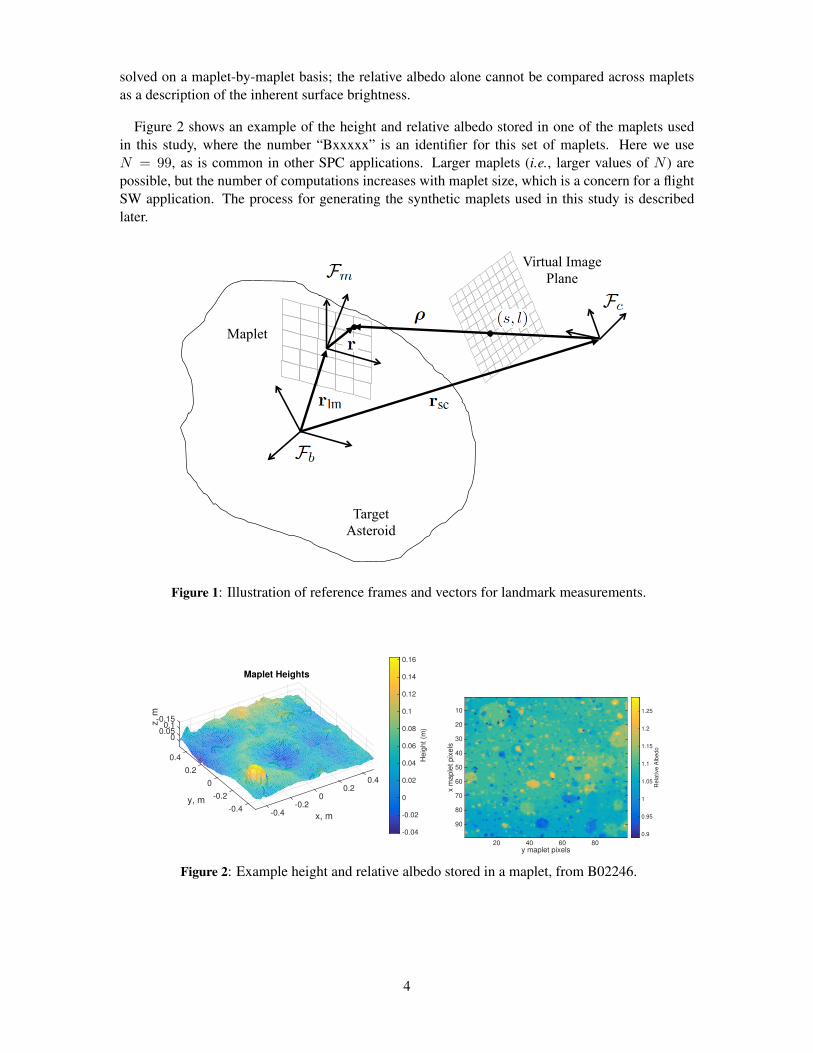
It is useful to first define some terminology and variables used in the SPC and landmark templatematching process before describing the overall conops flow. The reference frame Fb is the targetasteroid’s body-fixed frame (see Figure 1). The asteroid surface map is divided into a series ofmaplets that tile the surface (with partial overlaps allowed). The SPC literature sometimes refers tomaplets as “L-maps” as well.3 Below is a list of some of the properties of a maplet, all of which aredefined in the maplet creation process of SPC:

• Landmark – the center (origin) of a given maplet is denoted as a landmark, with a positionvector rlm relative to the target body. Note that the landmark itself does not have to be adistinguishing feature, such as a boulder or crater; it is the surrounding maplet terrain’s heightand albedo that form our required image templates. In other words, the maplet terrain itselfmust have a certain amount of variation.

• Maplet Frame – the local coordinate frame centered on the landmark, Fm, where the z-axispoints towards zenith. The orientation of Fm relative to Fb is known.

• Maplet Grid Resolution and Scale – the number of grid elements that define the maplet (i.e.,N × N ), and the scale of each maplet grid element (i.e., meters per element). Note that theterm “maplet pixel” is sometimes used as well to describe a maplet grid element, but cancause confusion with image pixels.

• Maplet Space Coordinate - the cartesian position r = (x, y, z) that describes a point in themaplet Fm.

• Height – an N × N matrix of height values that is a function z = z(x, y) of planar gridcoordinates in Fm.

• Relative Albedo– an N × N matrix of albedo values, also a function a = a(x, y) of mapletplanar grid coordinates in Fm.

The albedo contained in the maplet is not an absolute albedo; it is a relative albedo because it isa description of a given maplet element’s surface material brightness relative to that of all otherelements in that maplet. For example, if points A and B in a maplet have a(xA, yA) = 1 anda(xB, yB) = 2, then point B is twice as bright as point A (assuming they have equal slopes andSun-observer geometry). Hence, the relative albedo is only meaningful when used with the assumedillumination model, discussed below. In the SPC maplet construction process, the relative albedo is

3

solved on a maplet-by-maplet basis; the relative albedo alone cannot be compared across mapletsas a description of the inherent surface brightness.

Figure 2 shows an example of the height and relative albedo stored in one of the maplets usedin this study, where the number “Bxxxxx” is an identifier for this set of maplets. Here we useN = 99, as is common in other SPC applications. Larger maplets (i.e., larger values of N ) arepossible, but the number of computations increases with maplet size, which is a concern for a flightSW application. The process for generating the synthetic maplets used in this study is describedlater.

Virtual Image Plane

Maplet

Target Asteroid

Figure 1: Illustration of reference frames and vectors for landmark measurements.

0.40.2

x, m

0

Maplet Heights

-0.2-0.4

-0.4

-0.2

0

y, m

0.2

0.4

0.150.1

0.050

z,

m

He

igh

t (m

)

-0.04

-0.02

0

0.02

0.04

0.06

0.08

0.1

0.12

0.14

0.16

Maplet Relative Albedo

y maplet pixels20 40 60 80

x m

ap

let

pix

els

10

20

30

40

50

60

70

80

90

Rela

tive A

lbedo

0.9

0.95

1

1.05

1.1

1.15

1.2

1.25

Figure 2: Example height and relative albedo stored in a maplet, from B02246.

4

Transformation from Maplet Space to Image Space

Figure 1 shows the vector relationship

rlm + r− rsc = ρ (1)

where rsc is the spacecraft position vector relative to the Fb origin, and ρ is the position vector ofa surface point in the maplet relative to the camera focal point centered on the camera frame Fc.Note that in the remainder of this study, we ignore the offset of the camera relative to the spacecraftbody center. Also, we ignore errors in knowledge of the camera position and orientation relativeto the spacecraft, and in essence treat the spacecraft as consisting of nothing but the camera. TheLOS vector to a surface point is then ρ = ρ/||ρ||. Considering a virtual image plane in front ofthe focal point, then the point of intersection between ρ and this plane is described by image spacecoordinates (s, l), which are the (sample,line) coordinates in the image∗.

The optical model follows Reference 17. The nonlinear measurement model that describes the(s, l) measurements to a surface point r = (x, y, z) as a function of the spacecraft pose x (i.e.,position and attitude), modeled landmark position rlm, and vector of camera model parameters c isdenoted [

sl

]= h(x, rlm, c) (2)

In other words, h() is the transformation that maps a point in maplet space to a point in image space.The steps involved in Eq. 2 are as follows. The position vectors in Eq. 1 are initially expressed inFb,

rblm + rb − rbsc = ρb (3)

The vector ρb is then rotated into Fc using the assumed camera attitude knowledge between Fb andFc:

ρc = Rb→cρb (4)

The 2D gnomonic projection (i.e., pinhole camera model) gives the coordinates z =[zx zy

]T inmm on the virtual image plane:

z =f

ρc3

[ρc1ρc2

](5)

where f is the focal length and ρc =[ρc1 ρc2 ρc3

]T . A model for geometrical distortion (i.e.,deviations from a simple pinhole camera optical model) is then applied:

z′ = z +

[−zyr zxr

2 −zyr3 zxr4 zxzy z2x

zxr zyr2 zxr

3 zyr4 z2y zxzy

]ε (6)

where r = ||z||, and ε =[ε1 · · · ε6

]T are the parameters that describe the distortion due to2nd-order radial distortion and tangential distortion. The coordinates on the distorted virtual imageplane z′ =

[z′x z′y

]Tare still expressed in mm; the mapping to pixel coordinates (s, l) is achieved

with [sl

]= K

[z′

1

](7)

∗The (sample,line) measurements are synonymous with the (column,row) notation for describing the pixel coordinatesin a image.

5

where the matrix

K =

[Kx Kxy s0Kyx Ky l0

](8)

contains the image pixel coordinates of the principle point (s0, l0) (i.e., where the camera boresightintersects the image plane), the terms Kx and Ky convert from units of mm to pixels, and the termsKxy and Kyx apply a rotation. We can now define the vector of camera model parameters in Eq. 2as c = (f, ε,K).

PROCESS OVERVIEW

This section describes the overall optical navigation process in conjunction with the TRN phaseof the mission (see Figure 3). The major components in the landmark template matching processare described in the following subsections. This paper does not go into detail on the other elementsof the planned onboard GN&C process, such as the filter, controller, guidance algorithms, and statepropagation.

Figure 3: Flow chart of SPC, Retina, and optical GN&C processes.

The ground-based SPC functionality shown in Figure 3 is assumed to be nearly identical to thesystem used in previous SPC missions, as discussed above in the introduction. One set of inputs tothe ground-based SPC is the narrow field-of-view (FOV) survey images taken from a higher map-ping altitude. The outputs of the SPC process are the individual maplets. Furthermore, the groundsystem will include a landmark down-selection algorithm responsible for taking the predicted space-craft ephemeris and attitude pointing and choosing the appropriate L-maps to be uploaded to the

6

vehicle.

The inputs to the landmark template matching process are: the maplets generated during theground-based SPC process, the predicted spacecraft state at the current time from the onboardGN&C subsystem, and the current wide-FOV imagery from the onboard optical navigation cam-era. The landmark template matching is usually performed in an iterative fashion, where an initialguess of the landmark LOS vector is refined. For the initial iteration into the template matchingloop (i = 0), an initial estimate of the (s, l) measurement to the landmark is computed using the apriori pose estimate x∗ and the model from Eq. 2:[

sl

]i=0

= h(x∗, rlm, c) (9)

Landmark Extraction from Image

In this step, the portion of the image that contains the maplet data is identified, and those imagepixels are transformed from image space into maplet space, i.e., the maplet data is extracted fromthe image. The main steps for accomplishing the image extraction are as follows:

• Compute the Jacobian of h() with respect to r evaluated on (x∗, rlm, c) using finite differenc-ing:

H =∂h()

∂r

∣∣∣∣(x∗,rlm,c)

(10)

• Loop over each point rk in maplet space, where k ∈ {1, · · · , N2}, and project that point intoimage space (s, l) using the linearization[

sl

]k

=

[sl

]i

+ Hrk (11)

• The image data must be interpolated at the projected point, because the projected point inimage space almost certainly will not fall exactly on an image pixel (recall Figure 1). Thisimage interpolation is nominally performed with bilinear interpolation.

• Iterate around the maplet point rk using a small search distance, and for each of these addi-tional points in maplet space, repeat the above-mentioned projection and interpolation steps.The purpose of this additional iteration is to perform local averaging of the computed bright-ness.

• Loop over each point in the extracted image and normalize the brightness within the maxi-mum detector thresholds. Denote the final extracted image intensity at maplet coordinate kas Iext(k). See Figure 4a for an example of an extracted maplet image, where the color scaledenotes the normalized image intensity.

Predicted Maplet Rendering

The L-map data is illuminated using knowledge of the slope and albedo at each point, as well asthe sun direction and assumed spacecraft pose. This predicted brightness I at each point k in theL-map is calculated using an illumination model that has been developed over the years for airless

7

extracted image of maplet

y (maplet grid elements)0 20 40 60 80 100

x (

ma

ple

t g

rid

ele

me

nts

)

10

20

30

40

50

60

70

80

90

0

0.1

0.2

0.3

0.4

0.5

0.6

0.7

0.8

0.9

1

(a)

predicted image of maplet


x (

ma

ple

t g

rid

ele

me

nts

)

10

20

30

40

50

60

70

80

90

0

0.2

0.4

0.6

0.8

1

(b)

Figure 4: Left (a) example of extracted maplet image from L-map B02246, right (b) example ofpredicted maplet image from L-map B02246.

planetary bodies. Let s denote the sun direction unit vector in Fm, and let e denote the emissiondirection unit vector in Fm (i.e., the direction from the surface to the observer). Let the surfacenormal vector at r in Fm be n. Then the incidence angle, emission angle, and phase angle are givenrespectively with

i = cos−1(s · n) (12)

e = cos−1(e · n) (13)

α = cos−1(s · e) (14)

The function to calculate the predicted brightness at maplet coordinate rk is3

Ipred(k) = Λa(xk, yk)R(cos i, cos e, α) + Φ (15)

where Λ is an image scaling multiplier, a(xk, yk) is the relative albedo defined previously, Φ is apositive background term that can be used when there is background or haze in an image (e.g., due toambient lighting on a planet containing an atmosphere16), and R is the so-called “Lunar-Lambert”function defined as:18

R(cos i, cos e, α) = (1− L(α)) cos i+L(α) cos i

cos i+ cos e(16)

where the term L(α) is defined shortly. The Lunar-Lambert function is a combination of Lambertand Lommel-Seeliger reflectance functions, and is a simple model of single and multiple scattering,in which the scattering is isotropic. The term L(α) is a phase adjustment term to model limb-darkening. Reference 19 empircally models L(α) by fitting lunar data to a 3rd order polynomial.However, we follow the convention of Gaskell3 which does an additional fit using an exponential asfollows:

L(α) = exp(−α/60) (17)

where α is expressed in degrees. Note that the limb-darkening term L(α) is the only phase-dependent term in the intensity calculation. The Lunar-Lambert function of Eq. 16 has been vali-dated on powdery materials in the laboratory, as well as disk-integrated properties of asteroids andnatural satellites,18 not to mention the flight programs where SPC has been used in the past.

The steps for computing the predicted maplet brightness are as follows:

8

• Given the current spacecraft state inFb, compute the following vectors inFm: sun unit vector(s), and unit vector from maplet center to camera (e). Note that the simplification is madewhere e is assigned to be the same for all points in the maplet, and to take on the value fromthe maplet origin.

• Because the maplet contains the height data and not the slope data, the slope must be com-puted from the height. This is done by looping over each point in the maplet and computingthe slope in two directions with a finite differencing.

• Also in the loop over all points in the maplet, the illumination is calculated with Eq. 15. Theresult is the predicted illuminated maplet in Fm.

The illumination model used for the predicted images for this version of the landmark templatematching does not realistically account for shadowing, i.e., a full-fledged ray tracing is not per-formed. Instead, in the interest of computational speed, a maplet pixel is calculated as being darkonly if its incidence angle is greater than 90 degrees. This shadow modeling difference can be seenby comparing Figures 4a and 4b. This approximation is a hold-over from the original SPC andautoregister formulation, and its speed makes it desired for onboard image rendering. The impli-cations of this modeling approach on the correlation step, as well as future enhancements to thismethodology, are discussed below.

Correlation and Peak Finding

This step attempts to solve for the translational shift in maplet space ∆ri = (∆x,∆y) thatmaximizes the correlation between the predicted and extracted maplet images, where i is the cur-rent iteration of the template matching loop. If the onboard maplets contained no model errors andperfectly represented the true terrain, and if the camera model contained no errors, then only naviga-tional offsets (i.e., differences between the true and assumed spacecraft pose) would be responsiblefor non-zero values of ∆ri in this correlation step. By solving for the shift ∆ri using our a prioriknowledge of the spacecraft pose, we can adjust our a priori knowledge of the LOS vectors to thelandmarks.

Figure 5a is a simplified illustration of the process for correlating the predicted and extractedmaplets. In this simple example for easy visualization, the maplet has dimensions of 5 × 5 mapletpixels, and the correlation search is performed over a 3 × 3 grid. The predicted maplet is depictedin blue, the extracted maplet is depicted in yellow, and the overlapping regions are shown in green.The correlator is looped over the maplet-space planar search dimensions (∆x,∆y), and for a givenvalue of overlap, a correlation metric is computed and stored in a matrix as shown. The correlationmetric currently used is simply a linear correlation coefficient (i.e. the Pearson product momentcoefficient):

ρ =

∑IextIpred −

∑Iext∑Ipred√[

M∑I2ext − (

∑Iext)

2] [M∑I2pred −

(∑Ipred

)2] (18)

where M is the length of both signals Iext and Ipred. The correlation coefficient ρ is defined from -1(perfect inverse correlation) to 1 (perfect correlation).

Once the correlator loop has fully populated the correlation matrix, a peak correlation value isfound. The peak is found by selecting points on both sides of the max and finding the intersection

9

Δx = -1 horiz. shifts Δy = 1 vert. shifts

Δx = 0 horiz. shifts Δy = 1 vert. shifts

Δx = 1 horiz. shifts Δy = 1 vert. shifts

…

Correlation matrix of ρ(Δx, Δy)

(a)

Horizontal shift "x0 5 10

Ver

tical

shi

ft "

y

2

4

6

8

10

Cor

rela

tion

coef

ficie

nt ;

0.2

0.3

0.4

0.5

0.6

0.7

0.8

(b)

Figure 5: Left (a) shows a simplified illustration of the process for populating the correlation matrixρ(∆x,∆y). Right (b) is an example of the ρmatrix using Ipred and Iext from our descent simulations.

of lines constructed from those points, where the slopes of the lines are computed from the corre-lation matrix gradient. The solution ∆ri is the shift that maximizes the correlation coefficient. Thecorrelation search distances are controlled by the template matching loop iteration, e.g. ∆x = 5Li,where Li in the current simulations begins at a max of 10 and decrements to 1. Hence, the search isinitially performed over a larger area in maplet space and should converge to a small area. Note thatthe peak finding in the ρ matrix allows sub-maplet-pixel solutions for ∆ri. Figure 5b is an exampleof the ρ correlation matrix using the predicted and extracted maplets (from an unperturbed case)from our ARRM descent simulations, where the correlation matrix has dimensions of 11× 11.

It is important to note that the correlated images from the predicted and extracted maplets aredecomposed into a one-dimensional signal, hence all spatial information is lost, and the correla-tion is performed on a pixel-by-pixel basis. Also, because the illumination model for the predictedmaplets is known to be deficient with regard to shadow calculations (as mentioned above), a pairof image pixels from the predicted and extracted maplets is included in the correlation signal onlyif both are greater than a near-zero threshold. In other words, the correlator is intentionally disre-garding shadowed pixels in either image. Lastly, the linear correlation coefficient ρ is invariant tolinear transformations of one signal relative to the other; for example, the slight differences in thenormalized image intensities between Iext and Ipred apparent in the color scales in Figures 4a and 4bdo not affect ρ.

Image Space Transformation

Lastly, the landmark LOS shift measurements are transformed from maplet space into imagespace, again using the a priori spacecraft state knowledge. Here, the linearized transformation isused again: [

sl

]i+1

=

[sl

]i

+ H∆ri (19)

If the template matching loop is done with all iterations i, then the final landmark LOS measure-ments (s, l) can be fed into the onboard GN&C filter, otherwise the loop repeats.

10

SIMULATION ENVIRONMENT

An in-house renderer called Geomod is used to model the 3D scene geometry, lighting models,and ray tracing for synthesizing the “truth” images in our ARRM simulations. The ray tracer usesMonte Carlo importance sampling to follow a large number of incoming light ray directions (back-wards) from a pixelated detector grid, through a lens system, and into a scene. It is physically-basedon radiometric light transport, geometric optics, and statistically unbiased Monte Carlo integration.Geomod has been used previously to support simulations of the Origins, Spectral Interpretation,Resource Identification, Security, Regolith Explorer (OSIRIS-REx) mission.

For the purposes of this study, the wide-FOV navigation camera is baselined using similar pa-rameters as the NAVCAM wide-FOV camera on OSIRIS-REx (see Table 1). From Table 1, theprinciple point pixel coordinates are (s0, l0) = (1296.5, 972.5), and Kx = 454.54, Ky = −454.54,and Kxy = Kyx = 0.

Table 1: Wide-FOV camera parameters used in this study

Parameter Value

Detector horizontal resolution 2592 pixelsDetector vertical resolution 1944 pixelsFocal length, f 7.68 mmDetector pixel dimensions 2.2 × 2.2 micronsCamera horizontal FOV 40.7 degCamera vertical FOV 31.1 deg

There are two sets of maplets for the asteroid surface used in this study. The first is the “truth”set used to render the synthetic images from Geomod, which has 3-mm resolution maplet pixels.The onboard maplet set (i.e., the maplets we assume would be used onboard during the descentfrom 50-m altitude, denoted with the “B” prefix) is derived from the truth set for the purposes ofthis simulation∗, but is down-sampled and smoothed to a final maplet pixel resolution of 1-cm, withN = 99. The down-sampling and smoothing from truth maplets to onboard maplets introducessmall systematic errors (e.g., on the order of a few cm in height).

The asteroid surface is simulated with a suite of FORTRAN algorithms provided by Gaskell,which take as input an approximate shape model and applies a stochastic interpolation to add a re-alistic distribution of surface boulder, craters, and accretion layer. Earlier examples of this method-ology can be found in References 20 and 21. For example, the cratering distribution is based ona power law relating the number of craters and their diameters, as observed in nature. The out-put is a series of maplets at the desired resolution and scale. Gaskell5 shows an example of thesynthetic shape generation algorithms being applied to Bennu for the OSIRIS-REx mission. Fig-ure 6 shows the synthesized asteroid surface within the FOV at 50 m altitude, with 12 landmarksindicated, where the magenta squares indicate the size of each individual maplet. Note that eachmaplet considered here is 1 m × 1 m, whereas the entire FOV at 50 m altitude covers an area onthe surface of approximately 28 m × 37 m. Figure 7 shows the extracted maplet images for each ofthe 12 landmarks at 50 m altitude. The reference trajectory for the ARRM vehicle’s descent to thesurface is the same as that used in Reference 22. Note that our simulation of the landmark matchingalgorithms in the present paper is not a dynamic simulation that uses the landmark measurements in

∗During actual operations, the onboard maplets come from the SPC process as described above, because obviouslythe truth terrain is unknown.

11

a closed loop; instead we simply use the vehicle’s asteroid-relative state a given time to render thetruth images and measure the landmarks.

PERFORMANCE CHARACTERIZATION

This section describes the results of running the landmark template matching algorithms whensubjected to imperfect knowledge of the spacecraft navigational state and model parameters (i.e.,parameters affecting both the camera model and terrain model).

Perturbed cases at 50 m altitude

The nominal states and model parameters were perturbed at 50-m altitude from the surface as de-scribed in Table 2. Each perturbation is zero-mean and normally distributed with the 1-σ standarddeviations shown. Most of the perturbation values in the table are realistic assumptions at this stageof the preliminary design, with the exception of the spacecraft pose knowledge relative to the as-teroid, as discussed below. The landmark template matching algorithms were simulated in a MonteCarlo (MC) setting, with Latin Hypercube Sampling (LHS)23 of 500 samples per landmark. LHSgenerally allows a more accurate representation of the desired probability density function compared

Image line, pixels-500 0 500 1000 1500 2000 2500

Ima

ge

sa

mp

le,

pix

els

500

1000

1500

2000

2500

B01980

B02176

B02246

B01585

B01909B02235

B02690

B02631

B02642

B01926

B01536

B01595

Figure 6: Synthetic image of asteroid surface from Geomod at 50-m altitude, showing location ofthe 12 landmarks used in the performance characterization.

12



x (

ma

ple

t g

rid

ele

me

nts

)

10

20

30

40

50

60

70

80

90

0

0.1

0.2

0.3

0.4

0.5

0.6

0.7

0.8

0.9

1

(a) B01980



x (

ma

ple

t g

rid

ele

me

nts

)

10

20

30

40

50

60

70

80

90

0

0.1

0.2

0.3

0.4

0.5

0.6

0.7

0.8

0.9

1

(b) B02176



x (

ma

ple

t g

rid

ele

me

nts

)

10

20

30

40

50

60

70

80

90

0

0.1

0.2

0.3

0.4

0.5

0.6

0.7

0.8

0.9

1

(c) B02246extracted image of maplet


x (

ma

ple

t g

rid

ele

me

nts

)

10

20

30

40

50

60

70

80

90

0

0.1

0.2

0.3

0.4

0.5

0.6

0.7

0.8

0.9

1

(d) B01585



x (

ma

ple

t g

rid

ele

me

nts

)

10

20

30

40

50

60

70

80

90

0

0.1

0.2

0.3

0.4

0.5

0.6

0.7

0.8

0.9

1

(e) B01909



x (

ma

ple

t g

rid

ele

me

nts

)

10

20

30

40

50

60

70

80

90

0

0.1

0.2

0.3

0.4

0.5

0.6

0.7

0.8

0.9

1

(f) B02235extracted image of maplet


x (

ma

ple

t g

rid

ele

me

nts

)

10

20

30

40

50

60

70

80

90

0

0.1

0.2

0.3

0.4

0.5

0.6

0.7

0.8

0.9

1

(g) B02690



x (

ma

ple

t g

rid

ele

me

nts

)

10

20

30

40

50

60

70

80

90

0

0.1

0.2

0.3

0.4

0.5

0.6

0.7

0.8

0.9

1

(h) B02631



x (

ma

ple

t g

rid

ele

me

nts

)

10

20

30

40

50

60

70

80

90

0

0.1

0.2

0.3

0.4

0.5

0.6

0.7

0.8

0.9

1

(i) B02642extracted image of maplet


x (

ma

ple

t g

rid

ele

me

nts

)

10

20

30

40

50

60

70

80

90

0

0.1

0.2

0.3

0.4

0.5

0.6

0.7

0.8

0.9

1

(j) B01926



x (

ma

ple

t g

rid

ele

me

nts

)

10

20

30

40

50

60

70

80

90

0

0.1

0.2

0.3

0.4

0.5

0.6

0.7

0.8

0.9

1

(k) B01536



x (

ma

ple

t g

rid

ele

me

nts

)

10

20

30

40

50

60

70

80

90

0

0.1

0.2

0.3

0.4

0.5

0.6

0.7

0.8

0.9

1

(l) B01595

Figure 7: Extracted maplet images (Iext) for the 12 L-maps at 50-m altitude.

with MC for the same number of samples. LHS was chosen because the landmark image process-ing algorithms are currently implemented in Matlab, hence a large number of MC samples requirea long computation time. The “truth” measurement (s, l)truth is defined as Eq. 2 evaluated on theunperturbed values of (x, rlm, c), the “perturbed” (s, l)perturb is the result of the landmark templatematching algorithms when (x, rlm, c) are perturbed, and the resulting errors in the measurement asa result of the perturbations are (s, l)err = (s, l)truth − (s, l)perturb. Note that the synthesized images(simulated from the navigation camera) are not re-rendered for each perturbed sample due to thelong computational time required; rather we are perturbing our knowledge of the navigation state

13

and model parameters for a single set of collected (i.e., synthesized) images. Additional fidelitymay be achieved in future simulations that also perturb the truth state (as well as rendered syntheticimagery).

Table 2: Monte Carlo Simulation Parameters

Parameter or state to perturb 1-σ std applied

Asteroid-relative spacecraft position rsc, each component 0.1667 mAsteroid-relative spacecraft attitude, each component 0.05 degAsteroid-relative landmark position rlm, each component 3.33 cmMaplet terrain height z(x, y) 3.33 mmMaplet terrain albedo a(x, y) 0.047Camera model pixel skew Kyx 1× 10−5

Camera model principle coordinates (s0, l0) 0.1667 pixelsCamera model focal length f 0.004 mmCamera model distortion coefficients ε (1× 10−5, 1× 10−7, 1× 10−5, 1× 10−5, 0, 0)Asteroid-relative sun vector direction, RA and DEC 0.3 deg

The results of the LHS simulations are summarized in Table 3, and Figure 8 shows the distributionin (s, l)err for each landmark. The first column in the table is the landmark ID number. The nextfour columns are the means and 1-σ standard deviations of (s, l)error. The 6th column shows thenumber of samples where a peak in the correlation matrix was not found, e.g., due to the peak beingon the edge of the search distance, or the correlation matrix not showing a clearly defined peak. The7th column shows the number of samples where the peak correlation was found, but with a valuebelow a specified threshold of 0.3. The threshold level was determined based on experience in thesimulations, but this value is subject to change. The 8th column is the landmark template matchingsuccess rate, meaning the fraction of those 500 samples that successfully had a peak correlationvalue above the 0.3 threshold. The last column is the mean across the 500 samples of the maxcorrelation value ρ from the correlation matrix from each sample. The samples shown in Figure 8correspond to those having a successfully located correlation peak. From these results, it is clearthat these 12 landmarks have a line error lerr mean close to zero, but a small bias of approximately-0.1 pixels in the sample error serr. The error distributions shown in Figure 8 do not show any strongnon-Guassian behavior. The lerr 1-σ std is consistently larger than the corresponding statistic in serr,but both are below approximately 0.1 image pixels.

The biggest influences on the size of the errors (s, l)err are the knowledge errors in spacecraftpose, followed to a lesser extent by rlm, (s0, l0), and z(x, y). The majority of the failure cases in thelandmark template matching (i.e., the approximately 10% of the 500 samples for each landmark)are due to the spacecraft pose knowledge errors projecting the extracted maplet imagery too faroff of the maplet terrain in maplet space. Recall from the discussion on the correlation in mapletspace, that the correlation is only performed on the overlapping portions of the two signals. As thecorrelation signal size decreases, the quality of the linear correlation quickly degrades (especiallyin the presence of noise). Considering the 1-σ values, the spacecraft position alone is 0.17 m andthe attitude is 0.05 deg; when these two act in the same direction (parallel to the asteroid surface)the result is an offset in the boresight intersection with the asteroid surface of roughly 42 cm atthe 2-σ level. The max search distance used in the correlation loop for these tests is L = 10,corresponding to a maplet space max search distance of 5L = 50 maplet pixels, or 50 cm. Hence,when the spacecraft pose knowledge errors approach the 2-σ levels, the correlation algorithm beginsto approach its maplet space search distance limits when L = 10.

14

sample error-0.35 -0.3 -0.25 -0.2 -0.15 -0.1 -0.05 0 0.05

line

err

or

-0.2

-0.1

0

0.1

0.2

0.3

0.4

B01980.MAP, frame=0 Mean=[ -0.136, 0.048 ] pix, Std=[ 0.062 , 0.096] pix

Total Runs=500, Not Found=42, Sub-threshold(0.30)=1520151110120837

(a) B01980

sample error-0.3 -0.25 -0.2 -0.15 -0.1 -0.05

line

err

or

-0.1

-0.05

0

0.05

0.1

0.15

0.2



(b) B02176

sample error-0.25 -0.2 -0.15 -0.1 -0.05 0 0.05

line

err

or

-0.25

-0.2

-0.15

-0.1

-0.05

0

0.05

0.1

0.15

0.2

B02246.MAP, frame=0 Mean=[ -0.111, -0.027 ] pix, Std=[ 0.041 , 0.082] pix


(c) B02246

sample error-0.15 -0.1 -0.05 0 0.05

line

err

or

-0.15

-0.1

-0.05

0

0.05

0.1

0.15

0.2

0.25



(d) B01585

sample error-0.2 -0.15 -0.1 -0.05 0 0.05 0.1

line

err

or

-0.15

-0.1

-0.05

0

0.05

0.1

0.15

0.2

0.25

0.3



(e) B01909

sample error-0.25 -0.2 -0.15 -0.1 -0.05 0

line

err

or

-0.15

-0.1

-0.05

0

0.05

0.1

0.15

0.2

0.25



(f) B02235

sample error-0.2 -0.15 -0.1 -0.05 0 0.05 0.1

line

err

or

-0.4

-0.3

-0.2

-0.1

0

0.1

0.2



(g) B02690

sample error-0.25 -0.2 -0.15 -0.1 -0.05 0

line

err

or

-0.25

-0.2

-0.15

-0.1

-0.05

0

0.05

0.1

0.15



(h) B02631

sample error-0.3 -0.25 -0.2 -0.15 -0.1 -0.05 0 0.05

line

err

or

-0.4

-0.3

-0.2

-0.1

0

0.1

0.2

0.3

0.4



(i) B02642

sample error-0.3 -0.25 -0.2 -0.15 -0.1

line

err

or

-0.15

-0.1

-0.05

0

0.05

0.1

0.15

0.2



(j) B01926

sample error-0.3 -0.25 -0.2 -0.15 -0.1

line

err

or

-0.1

-0.05

0

0.05

0.1

0.15

0.2

0.25

0.3



(k) B01536

sample error-0.25 -0.2 -0.15 -0.1 -0.05 0 0.05

line

err

or

-0.1

-0.05

0

0.05

0.1

0.15

0.2

0.25

0.3



(l) B01595

Figure 8: Monte Carlo results from several landmarks at 50-m altitude, where the axes are (s, l)errin units of image pixels.

15

Table 3: Summary of Monte Carlo (LHS) Simulation Results at 50 m altitude.

L-mapID

Sampleerrormean[pix]

Lineerrormean[pix]

Sampleerrorstd[pix]

Lineerrorstd[pix]

Num.notfound

Num.belowthresh.

SuccessRate

Meanof maxρ

B01980 -0.136 0.048 0.062 0.096 42 15 0.89 0.54B02176 -0.163 0.053 0.028 0.066 23 25 0.90 0.54B02246 -0.111 -0.027 0.041 0.082 31 18 0.90 0.58B01585 -0.041 0.054 0.033 0.082 36 20 0.89 0.56B01909 -0.049 0.081 0.043 0.085 36 15 0.90 0.55B02235 -0.139 0.068 0.025 0.071 39 12 0.90 0.55B02690 -0.052 -0.056 0.043 0.097 52 16 0.86 0.57B02631 -0.107 -0.069 0.038 0.076 37 13 0.90 0.57B02642 -0.117 0.007 0.058 0.113 46 15 0.88 0.58B01926 -0.193 0.019 0.032 0.078 49 6 0.89 0.59B01536 -0.208 0.118 0.037 0.083 35 19 0.89 0.58B01595 -0.114 0.111 0.041 0.080 33 25 0.88 0.57

The descent GN&C conops currently assumes the spacecraft pose navigational errors to be ap-proximately 0.5 m and 0.6 deg (3σ) in each component at 50 m altitude, based on a linear covari-ance analysis assuming landmark measurements (s, l) with 1σ noise of 1 pixel.22 Thus, we haveshown that the achievable landmark measurement noise may be smaller, but we have also assumeda smaller navigational error in attitude knowledge (recall Table 2). Thus, the current landmarktemplate matching algorithm and settings may be insufficient for accurately providing landmarkmeasurements with this level of spacecraft pose error, which requires further investigation. Onealternative is to increase the search distance L: the downside of this approach is the potential in-crease in computational burden as a larger search area must be iterated in the correlator. Anotheralternative is to increase the maplet template size (i.e., N ), which comes with its own increase incomputation burden because many of the calculation are performed on a pixel-by-pixel basis in themaplet. We are exploring a new approach to solving this problem by performing the correlations inimage space, as opposed to maplet space, described below in the discussion on Retina.

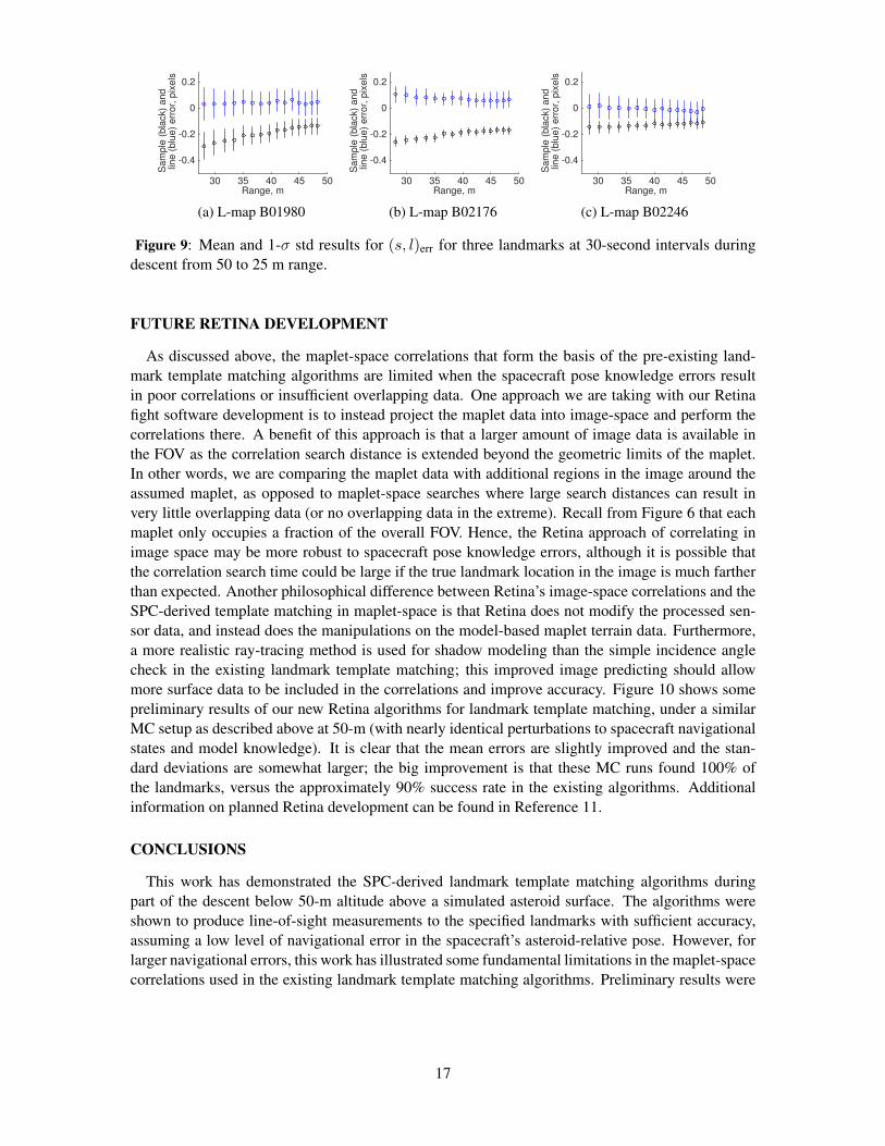
Perturbed cases during descent below 50-m altitude

The above perturbed cases were repeated for three landmarks at 30-second intervals during thedescent, beginning at 50-m altitude and stopping before 25-m altitude. Figure 9 shows these results,where the mean and 1-σ std from each 500-sample LHS run are shown as a box-and-whiskers plot.The sample and line errors are shown in black and blue, respectively. Note that each run of thelandmark template matching algorithm at a given instant is independent, i.e., the (s, l) solution atone time step is not used as an input to the next time step. Only three landmarks are shown herebecause of the large number of samples required to run the LHS simulations at this 30-secondtime step in Matlab. Figure 9 shows that the standard deviations do not increase greatly as thespacecraft approaches the surface. The largest increase here is the sample error mean and std forL-map B01980, which nearly double during the approach. Figure 7 shows that this landmark hastwo large boulders, unlike L-maps B02176 and B02246, and the boulder shadows exist mostly alongthe sample direction. One possible explanation for this error growth is mis-modeling of the bouldershadows in the predicted image (as described after Eq. 17). Lastly, it is worth noting that neither thelandmark template matching success rate nor the max correlation value changed significantly overthe altitude ranges tested.

16

Range, m30 35 40 45 50

Sam

ple

(bla

ck)

and

line (

blu

e)

err

or,

pix

els

-0.4

-0.2

0

0.2

L-map 1980

(a) L-map B01980

Range, m30 35 40 45 50

Sam

ple

(bla

ck)

and

line (

blu

e)

err

or,

pix

els

-0.4

-0.2

0

0.2

L-map 2176

(b) L-map B02176

Range, m30 35 40 45 50

Sam

ple

(bla

ck)

and

line (

blu

e)

err

or,

pix

els

-0.4

-0.2

0

0.2

L-map 2246

(c) L-map B02246

Figure 9: Mean and 1-σ std results for (s, l)err for three landmarks at 30-second intervals duringdescent from 50 to 25 m range.

FUTURE RETINA DEVELOPMENT

As discussed above, the maplet-space correlations that form the basis of the pre-existing land-mark template matching algorithms are limited when the spacecraft pose knowledge errors resultin poor correlations or insufficient overlapping data. One approach we are taking with our Retinafight software development is to instead project the maplet data into image-space and perform thecorrelations there. A benefit of this approach is that a larger amount of image data is available inthe FOV as the correlation search distance is extended beyond the geometric limits of the maplet.In other words, we are comparing the maplet data with additional regions in the image around theassumed maplet, as opposed to maplet-space searches where large search distances can result invery little overlapping data (or no overlapping data in the extreme). Recall from Figure 6 that eachmaplet only occupies a fraction of the overall FOV. Hence, the Retina approach of correlating inimage space may be more robust to spacecraft pose knowledge errors, although it is possible thatthe correlation search time could be large if the true landmark location in the image is much fartherthan expected. Another philosophical difference between Retina’s image-space correlations and theSPC-derived template matching in maplet-space is that Retina does not modify the processed sen-sor data, and instead does the manipulations on the model-based maplet terrain data. Furthermore,a more realistic ray-tracing method is used for shadow modeling than the simple incidence anglecheck in the existing landmark template matching; this improved image predicting should allowmore surface data to be included in the correlations and improve accuracy. Figure 10 shows somepreliminary results of our new Retina algorithms for landmark template matching, under a similarMC setup as described above at 50-m (with nearly identical perturbations to spacecraft navigationalstates and model knowledge). It is clear that the mean errors are slightly improved and the stan-dard deviations are somewhat larger; the big improvement is that these MC runs found 100% ofthe landmarks, versus the approximately 90% success rate in the existing algorithms. Additionalinformation on planned Retina development can be found in Reference 11.

CONCLUSIONS

This work has demonstrated the SPC-derived landmark template matching algorithms duringpart of the descent below 50-m altitude above a simulated asteroid surface. The algorithms wereshown to produce line-of-sight measurements to the specified landmarks with sufficient accuracy,assuming a low level of navigational error in the spacecraft’s asteroid-relative pose. However, forlarger navigational errors, this work has illustrated some fundamental limitations in the maplet-spacecorrelations used in the existing landmark template matching algorithms. Preliminary results were

17

presented on a different algorithmic approach, where terrain data is projected into image-space formore robust correlation. This different approach to landmark template matching is being developedas the Retina flight software for eventual onboard implementation.

Figure 10: Example Monte Carlo results from Retina, where column = sample and row = line.

ACKNOWLEDGEMENTS

This work was performed under NASA contract number NNG12CR31C. The authors acknowl-edge the support of the Satellite Servicing Capabilities Office. We thank Bob Gaskell of the Plan-etary Science Institute for his various SPC contributions, and Shaun Oborn and Reed McKenna ofSolo Effects LLC for their development of the Geomod image renderer. We also thank Alex Piniand Matt Vavrina of a.i. solutions, Inc. for reviewing a draft of this manuscript.

NOTATION

a maplet relative albedoc vector of camera model parameterse emission direction unit vectore emission angleFb asteroid body-fixed frameFc camera frameFm maplet framef camera focal lengthH Jacobian of h()

18

h() maplet-space to image-space transformationIext extracted image intensityIpred predicted image intensity

i (subscript) index of landmark matching loopi incidence angle

K camera intrinsic matrixKx,Ky camera mm-to-pixel scaling terms

Kxy,Kyx camera image rotation termsk (subscript) index of discrete point in maplet

L correlation search distanceL(α) limb-darkening phase adjustment termM length of vectors for correlationN number of maplet grid elements per siden surface normal direction unit vectorl line image coordinate, pixell0 line image coordinate of principle point, pixel

Rb→c rotation matrix from Fb to Fc

R Lunar-Lamber functionr position of point in maplet

rlm position of landmarkrsc position of spacecraft∆r solve-for shift in maplet spacer magnitude of zs sun direction unit vectors sample image coordinate, pixels0 sample image coordinate of principle point, pixelx spacecraft pose

x, y cartesian coordinates within maplet∆x,∆y cartesian components of ∆r

z virtual image plane coordinatesz′ distorted virtual image plane coordinatesz maplet height

zx, zy components of zα phase angleε vector of camera distortion coefficientsΛ image scaling multiplierρ range vector from camera to surface pointρ correlation value

ρ1, ρ2, ρ3 components of ρΦ positive background term

REFERENCES

[1] R. Merrill, M. Qu, M. Vavrina, J. Englander, and C. Jones, “Interplanetary Trajectory Design for the As-teroid Robotic Redirect Mission Alternate Approach Trade Study,” AIAA/AAS Astrodynamics SpecialistConference, San Diego, CA, 2014. AIAA 2014-4457.

19

[2] D. Reeves, B. Naasz, C. Wright, and A. Pini, “Proximity Operations for the Robotic Boulder CaptureOption for the Asteroid Redirect Mission,” AIAA Space 2014 Conference and Exposition, 4-7 Aug.2014, San Diego, CA, 2014. AIAA 2014-4433.

[3] R. Gaskell et al., “Characterizing and navigating small bodies with imaging data,” Meteoritics andPlanetary Science, Vol. 43, 2008, pp. 1049–1061.

[4] R. Gaskell, “Digital Identification of Cartographic Control Points,” Photogrammetric Engineering andRemote Sensing, Vol. 54, 1988, pp. 723–727.

[5] R. Gaskell, “Optical Navigation Near Small Bodies,” Advances in the Astronautical Sciences (M. K.Jah, Y. Guo, A. L. Bowes, and P. C. Lai, eds.), Vol. 140, 2011, pp. AAS 11–220.

[6] R. Gaskell, O. Barnouin-Jha, D. Scheeres, T. Mukai, N. Hirata, S. Abe, J. Saito, M. Ishiguro, T. Kubota,T. Hashimoto, J. Kawaguchi, M. Yoshikawa, K. Shirakawa, and T. Kominato, “Landmark NavigationStudies and Target Characterization in the Hayabusa Encounter with Itokawa,” AIAA/AAS Astrodynam-ics Specialist Conference and Exhibit, Keystone, Colorado, 2006.

[7] L. Jorda, P. L. Lamy, R. W. Gaskell, M. Kaasalainen, O. Groussin, S. Besse, and G. Faury, “Asteroid(2867) Steins: Shape, topography and global physical properties from OSIRIS observations,” Icarus,Vol. 221, No. 2, 2012, pp. 1089–1100.

[8] H. Sierks et al., “On the nucleus structure and activity of comet 67P/Churyumov-Gerasimenko,” Sci-ence, Vol. 347, No. 6220, 2015.

[9] N. Mastrodemos, B. Rush, D. Vaughan, and W. Owen, Jr., “Optical Navigation for the Dawn Mission,”23rd International Symposium on Space Flight Dynamics, Pasadena, CA, Oct 29 - Nov 2, 2012.

[10] A. S. Konopliv, S. W. Asmar, R. S. Park, B. G. Bills, F. Centinello, A. B. Chamberlin, A. Ermakov,R. W. Gaskell, N. Rambaux, C. A. Raymond, C. T. Russell, D. E. Smith, P. Tricarico, and M. T. Zuber,“The Vesta gravity field, spin pole and rotation period, landmark positions, and ephemeris from theDawn tracking and optical data,” Icarus, Vol. 240, 2013, pp. 103–117.

[11] C. Wright, M. Shoemaker, J. Van Eepoel, K. DeWeese, and K. Getzendanner, “Relative Terrain ImagingNavigation Tool (Retina) for the Asteroid Robotic Redirect Mission,” 39th AAS Guidance, Navigationand Control Conference, Breckenridge, CO, 2016. AAS 16-084.

[12] R. A. Schowengerdt, Remote Sensing (Third edition), ch. 8, pp. 355–385. Academic Press, 2007.[13] J. Riedel, T. Wang, R. Werner, A. Vaughan, and D. Myers, “Configuring the Deep Impact AutoNav Sys-

tem for Lunar, Comet, and Mars Landing,” AIAA/AAS Astrodynamics Specialist Conference, Honolulu,HI, 2008. AIAA 2008-6940.

[14] S. Bhaskaran, S. Nandi, S. Broschart, M. Wallace, L. Cangahuala, and C. Olson, “Small Body Land-ing Accuracy Using In-situ Navigation,” Advances in the Astronautical Sciences (K. B. Miller, ed.),Vol. 141, 2011, pp. AAS 11–056.

[15] S. Bhaskaran, “Autonomous Navigation for Deep Space Missions,” AIAA SpaceOps 2012 Conference,2012. doi:10.2514/6.2012-1267135.

[16] Y. Cheng, D. Clouse, A. Johnson, W. Owen, and A. Vaughan, “Evaluation and Improvement of PassiveOptical Terrrain Relative Navigation Algorithms for Pinpoint Landing,” Advances in the AstronauticalSciences (M. K. Jah, Y. Guo, A. L. Bowes, and P. C. Lai, eds.), Vol. 140, 2011, pp. AAS 11–221.

[17] W. Owen, “Methods of Optical Navigation,” Advances in the Astronautical Sciences (M. K. Jah, Y. Guo,A. L. Bowes, and P. C. Lai, eds.), Vol. 140, 2011, pp. AAS 11–215.

[18] A. McEwen, “Exogenic and Endogenic Albedo and Color Patterns on Europa,” Journal of GeophysicalResearch, Vol. 81, 1986, pp. 8077–8097.

[19] A. McEwen, “A Precise Lunar Photometric Function,” Lunar and Planetary Science, Vol. 27, 1996,pp. 841–842.

[20] R. Gaskell, “Martian Surface Simulations,” Journal of Geophysical Research, Vol. 98, 1993, pp. 11099–11103.

[21] R. Gaskell, J. Collier, L. Husman, and R. Chen, “Synthetic environments for simulated mis-sions,” Aerospace Conference, 2001, IEEE Proceedings., Vol. 7, 2001, pp. 7–3556 vol.7,10.1109/AERO.2001.931433.

[22] C. Wright, S. Bhatt, D. Woffinden, M. Strube, and C. D’Souza, “Linear Covariance Analysis for Prox-imity Operations Around Asteroid 2008 EV5,” 38th AAS Guidance, Navigation and Control Confer-ence, Breckenridge, CO, 2015. AAS 15-084.

[23] M. McKay, R. Beckman, and W. Conover, “A comparison of three methods for selecting values of inputvariables in the analysis of output from a computer code,” Technometrics, Vol. 21, 1979, pp. 239–245.

20

Documents

(Preprint) AAS 16-286 PERFORMANCE ...Preprint) AAS 16-286 PERFORMANCE CHARACTERIZATION OF A LANDMARK MEASUREMENT SYSTEM FOR ARRM TERRAIN RELATIVE NAVIGATION Michael A. Shoemaker, Cinnamon