Embed Size (px)
Citation preview

Freshwater dilution and transport in Canterbury Bight
Prepared for Environment Canterbury
June 2012

© All rights reserved. This publication may not be reproduced or copied in any form without the permission of the copyright owner(s). Such permission is only to be given in accordance with the terms of the client’s contract with NIWA. This copyright extends to all forms of copying and any storage of material in any kind of information retrieval system.
Whilst NIWA has used all reasonable endeavours to ensure that the information contained in this document is accurate, NIWA does not give any express or implied warranty as to the completeness of the information contained herein, or that it will be suitable for any purpose(s) other than those specifically contemplated during the Project or agreed by NIWA and the Client.
Authors/Contributors: Mark Hadfield John Zeldis
For any information regarding this report please contact:
Mark Hadfield Scientist Marine Physics +64-4- 386 0363 [email protected]
National Institute of Water & Atmospheric Research Ltd
301 Evans Bay Parade, Greta Point
Wellington 6021
Private Bag 14901, Kilbirnie
Wellington 6241
New Zealand
Phone +64-4-386 0300
Fax +64-4-386 0574
NIWA Client Report No: WLG2011-54 Report date: June 2012 NIWA Project: ENC11511 Cover images:
· MODIS true-colour image 7 September 2004, (Schwarz et al. 2008, figure A10).
· False-colour graph of freshwater concentration from a ROMS simulation, 17 June 2009 (this report)
· Sontek ADP

Freshwater dilution and transport in Canterbury Bight
Contents
Executive summary .............................................................................................................. 5
1 Introduction ................................................................................................................. 6
2 Methods: model setup ................................................................................................ 6
2.1 Nested domains ................................................................................................... 6
2.2 Freshwater input .................................................................................................. 9
2.3 Simulations ........................................................................................................ 11
3 Methods: field measurements .................................................................................. 11
3.1 CTD survey ........................................................................................................ 11
3.2 Current measurements ....................................................................................... 11
4 Model verification ...................................................................................................... 13
4.1 Sub tidal velocity ................................................................................................ 13
4.2 Tidal velocity ...................................................................................................... 16
4.3 Salinity ............................................................................................................... 16
5 Results ....................................................................................................................... 17
6 Discussion ................................................................................................................. 23
7 Acknowledgements ................................................................................................... 24
8 Glossary of abbreviations and terms ....................................................................... 25
9 References ................................................................................................................. 26
Appendix A Animations ................................................................................................... 28
Appendix B CTD-model comparisons ............................................................................ 29
Tables
Table 1: Model freshwater point sources. 9
Table 2: Sites for vertical profiles. 18
Figures
Figure 1: Model domains. 7
Figure 2: Freshwater flow rate time series. 10
Figure 3: Field measurement sites. 12
Figure 4: Currents at the outer ADP. 12

Freshwater dilution and transport in Canterbury Bight
Figure 5: Velocity scatter plot comparison at the outer ADP site. 14
Figure 6: Along-shore (60°T) velocity component comparison at the outer ADP site. 15
Figure 7: Cross-shore (330°T) velocity component comparison at the outer ADP site. 15
Figure 8: Tidal ellipse comparison for the outer (left) and inner (right) ADP sites. 16
Figure 9: Mean (upper) and maximum (lower) surface freshwater concentration . 20
Figure 10: Mean (upper) and maximum (lower) freshwater concentration at 10 m depth. 20
Figure 11: Sites for vertical profiles. 22
Figure 12: Profiles of mean and maximum freshwater concentration at six sites. 23
Reviewed by Approved for release by
……………………………………… ……………………………… Dr G. Rickard Dr A. Laing

Freshwater dilution and transport in Canterbury Bight 5
Executive summary
§ A nested set of ocean and coastal hydrodynamic models was set up with the
ultimate aim of simulating freshwater transport in Canterbury Bight and Pegasus
Bay.
§ A model of Canterbury Bight at 1 km resolution was run for a period of one year
(April 2009–April 2010), forced with ocean currents, winds, tides and freshwater
inputs from 10 rivers in Southland, Otago and Canterbury, along with Lake
Ellesmere/Te Waihora. The freshwater sources in Canterbury were each
labelled with a separate tracer, allowing the concentration of river-derived
freshwater to be evaluated and attributed to the specific source.
§ A programme of field measurements in Canterbury Bight has been carried out
under the same project, involving acoustic Doppler profiler (ADP) time series at
two locations and two surveys with conductivity-temperature-depth (CTD)
instruments, in July and December 2011.
§ The model produces freshwater plumes with behaviour that is physically
plausible and qualitatively consistent with remote sensing results.
§ The model verification confirms that the model is simulating currents in the area
very well and that the behaviour of the surface freshwater layer is realistic,
though it does not reproduce the small-scale variability on the in-shore transect
during the CTD surveys.
§ River plumes are initially confined very close to the surface (typically 1–3 m)
and have freshwater concentrations of 10–30%, occasionally approaching
100%. The plumes are progressively diluted by vertical mixing and horizontal
dispersion and form a coastal band ~10 km wide with surface freshwater
concentrations typically 5–10%.
§ The coastal freshwater band, and the river plumes within it, general move north-
eastward but with substantial fluctuations that are largely wind driven. Under
winds from the south or southwest, the coastal freshwater band can move quite
quickly (within a few days) north-eastward along the coast of Canterbury Bight
and around the end of Banks Peninsula.
§ The model indicates substantially higher freshwater concentrations on the
southern and eastern sides of Banks Peninsula than on the northern side.

26 Freshwater dilution and transport in Canterbury Bight
1 Introduction Environment Canterbury requires more information on the mixing and transport of
freshwater—with its associated nutrients, sediments and contaminants—entering Canterbury
Bight. A recent two-year study (Schwarz 2008,Schwarz et al. 2010) found that river plumes
were frequently visible in satellite images and were generally constrained to within 6 km or so
of the coastline. Water from Lake Ellesmere/Te Waihora was conspicuous because of its
yellow-green colour and was seen up to 95 km northeast and 27 km southwest of the source,
and up to 33 km from the coast. Plumes from the rivers and from Lake Ellesmere typically
moved north-eastward along the coast, around Banks Peninsula and into Pegasus Bay.
The task, as specified by Dr Lesley Bolton-Ritchie (‘Canterbury Bight water circulation and
mixing’. ECAN pers. comm., January 2010) was to model the near shore water circulation
and mixing processes in the Canterbury Bight with an emphasis on the fate of the freshwater
inputs to the Bight. This modelling was to investigate
§ the dilution and mixing of the freshwater inputs and
§ the offshore and alongshore movement of lower salinity water (resulting from
freshwater inputs).
The modelling must take into consideration the temporal variation in the volumes of
freshwater discharged into the Canterbury Bight.
This report describes modelling of the dynamics of freshwater-affected coastal waters. The
work has been accompanied by a programme of in-situ ocean observing for validation
purposes. This approach capitalises on the reciprocal relationship between modelling and in-
situ observation: the modelling allows prediction of the dynamics of freshwater-affected
waters under various environmental scenarios (e.g., wind, river flow patterns) over broader
time and space scales than can be achieved with in-situ observations, while the observations
validate predictions of the modelling.
The programme of field measurements in Canterbury Bight has now been completed. They
are described and compared with the model.
2 Methods: model setup
2.1 Nested domains
A nested set of hydrodynamic model domains was set up (Figure 1). The model used on all
three domains was ROMS1 (Haidvogel et al. 2008; MacCready et al. 2009), a widely used,
open-source ocean/coastal model. Coupling between the nested domains was one-way and
off-line: one-way because each domain influences any smaller-scale domains nested inside
it, but not vice versa and off-line because the models are run separately.
1 http://www.myroms.org/

Freshwater dilution and transport in Canterbury Bight 7
15 June 2012 4.31 p.m.
Figure 1: Model domains. (a) Outer and intermediate domains; (b) intermediate and inner domains; (c) inner domain with coastline (grey) and freshwater input locations (white symbols) shown over the land mask (light grey) and bathymetry (coloured) of the 1 km grid.

8 Freshwater dilution and transport in Canterbury Bight
The outer domain covered an area somewhat larger than the New Zealand EEZ at 10 km
resolution; the intermediate domain covered the continental shelf of the southeast South
Island at 2.5 km resolution; the inner domain covered Canterbury Bight and Pegasus Bay.
On the inner domain, model grids have been set up with two different resolutions: 1 km and
500 m; The simulations described here used 1 km grid and were run for a relatively long
time, namely one year. Because it is expensive—in terms of processor time and storage
space—to run simulations of comparable length with the 500 m grid, we intend in future to
compare simulations on the 1 km and 500 m grids for selected shorter periods (perhaps 20–
50 days) to establish whether the finer resolution changes the results significantly.
The outer model simulates the climatological2 large-scale flows around the New Zealand
landmass, essentially repeating the work of Rickard et al. (2005), but with a different model
code and different forcing datasets. Boundary conditions along the 4 sides of the outer model
grid were from a monthly climatology calculated from 10 years’ output of a global ocean
model (the SODA reanalysis, version 1.4.2, Carton and Giese 2008). The heat, momentum
and freshwater fluxes through the sea surface were from the NCEP Reanalysis monthly
climatology (Kalnay et al. 1996), with nudging of sea surface temperature (SST) towards a
monthly climatology from the NOAA optimum interpolation SST analysis (Reynolds et al.
2002). Weak nudging towards the SODA climatology was applied in the interior of the model
to prevent it drifting away from a realistic state. The outer model was spun up from rest for 3
years and then run for several more years, during which output was saved at 5 day intervals
and interpolated spatially to provide lateral boundary data for the intermediate model.
The intermediate model simulates the Southland Current, a flow of subtropical and
subantarctic water along the continental shelf of the south-eastern South Island (Sutton
2003). The Southland Current’s mean flow and water mass properties are imposed by the
outer model, and the intermediate model adds a much more accurate description of the
bathymetry and the ability to generate finer-scale turbulent flow structures (both permitted by
the finer grid) along with forcing by real-time winds. Freshwater sources representing the
major rivers are also included in the intermediate domain, as described in more detail in
Section 2.2.
The inner domain covers Canterbury Bight, Banks Peninsula and Pegasus Bay allowing the
inner model to simulate the movement of freshwater plumes in reasonable detail. The
Southland Current flows through this domain, imposed by the initialisation and lateral
boundary data derived from the intermediate model. Tides were imposed at the boundaries
of the inner domain in the form of 6 tidal constituents (M2, S2, N2, O1, K1, & P1) from the NIWA
EEZ tidal model (Stanton et al. 2001; Walters et al. 2001).
Given that the wind is known to be a major driver of variability in currents on the South Island
continental shelf (Chiswell 1996), the choice of wind data to drive the model is important. We
used 3-hourly winds from the NIWA NZLAM regional atmospheric model, which is part of the
EcoConnect3 environmental forecasting system. The NZLAM data are available from May
2007 to the present and appear to be superior to other wind datasets in their representation
of topographic effects by the New Zealand topography. Surface stresses were calculated
from the NZLAM winds using a standard relationship (Smith 1988) and then multiplied by a
2 There is an important distinction between climatological and real-time model forcing—see the glossary (Section 8).
3 http://ecoconnect.niwa.co.nz/

Freshwater dilution and transport in Canterbury Bight 9
15 June 2012 4.31 p.m.
factor of 1.2. This factor was adjusted to optimise the match between modelled and observed
sub tidal velocities (Section 4.1); similar adjustments have been found to be necessary in
other similar modelling exercises around New Zealand.
2.2 Freshwater input
The major rivers of the southern and eastern South Island, from the Oreti in Southland to the
Waimakariri in Pegasus Bay were represented in the model as point sources of freshwater
and also labelled with passive tracers, or “dyes”, as explained below. The freshwater sources
(the 10 rivers along with Lake Ellesmere) are listed in Table 1 column 1. The input locations
(Table 1 column 2) were established by inspecting Google Maps and then converted into
model grid locations, with adjustments to ensure each freshwater input lay on the model’s
land-sea boundary. Flow-rate time series were constructed for each source by multiplying
daily data from a suitable flow gauge site (Table 1 column 3) by a factor (Table 1 column 4)
representing the ratio between the total catchment area of the river (from the NIWA WRENZ4
site) and the catchment area upstream of the flow gauge site. For Lake Ellesmere, a daily
flow rate time series was constructed from opening/closing data for 2009–present supplied
by Graeme Horrell of NIWA, using the model described by Horrell (2009). The tracers
associated with each point source, or set of sources, are listed in Table 1 column 5. The four
rivers in Otago and Southland were all labelled with the same tracer, dye_01. The remaining
rivers, all in Canterbury, were labelled separately, with dye_02 to dye_08, giving a total of 8
tracers. Carrying this many tracers in the model simulations increases the resources required
substantially, but allows the individual plumes to be distinguished. The value of each dye
tracer was set to one in the water entering from its respective source(s) and zero elsewhere.
Thus the dye concentration in the model represents the volume fraction of river-derived
freshwater.
Table 1: Model freshwater point sources. See text for information on the construction of the time series.
Source Source input location Flow gauge Flow
factor
Tracer
Oreti 168.29318° E, 46.50395° S 78601 Oreti at Wallacetown 1.60
dye_01 Mataura 168.79735° E, 46.58187° S 77506 Mataura at Tuturau 1.23
Clutha 169.81067° E, 46.34515° S 75207 Clutha at Balclutha 1.00
Taieri 170.20257° E, 46.05358° S 74308 Taieri at Outram 1.21
Waitaki 171.14284° E, 44.93710° S 71110 Waitaki below Waitaki Dam 1.20 dye_02
Opihi 171.34998° E, 44.28165° S 69607 Opihi at No1 SHB 1.36 dye_03
Rangitata 171.51421° E, 44.18596° S 69302 Rangitata at Klondyke 1.21 dye_04
Ashburton 171.80366° E, 44.05293° S 68801 Ashburton at SHBr 1.01 dye_05
Rakaia 172.20661° E, 43.90176° S 68526 Rakaia at Fighting Hill 1.14 dye_06
Waimakariri 172.71054° E, 43.39133° S 66401 Waimakariri at Old Highway Br 1.10 dye_07
Ellesmere 172.37753° E, 43.85625° S dye_08
4 http://wrenz.niwa.co.nz/webmodel/

10 Freshwater dilution and transport in Canterbury Bight
The flow time series for the 8 tracers cover the years 2009 and 2010 (Figure 2), and will be
extended to the end of the measurement period in late 2011 as soon as the data become
available.
Figure 2: Freshwater flow rate time series.
The freshwater point sources were applied in the intermediate and inner domains only. (This
means that seawater entering the intermediate domain may be slightly more saline than it
should be, because the outer model is missing some freshwater inputs. However this is
expected to be a very small effect.) In the intermediate model, all 11 sources in Table 1 were

Freshwater dilution and transport in Canterbury Bight 11
15 June 2012 4.31 p.m.
included. In the inner domain, the first 4 sources lie outside the domain and so were omitted,
but the remaining 7 sources were included.
2.3 Simulations
Our strategy for simulations on the intermediate domain is to run a “base” simulation for a
several-year period, saving restart files at regular intervals from which other simulations can
be started as required. The base simulation in this case covered the years 2009–2011, with
restart files saved every 25 days. From the base simulation’s restart files, two shorter period
runs were conducted. The model output data from these runs comprised consecutive 0.5 day
averages throughout and these were then interpolated in space to provide lateral boundary
data for the inner model. The inner model was then run over the same periods.
The first inner model run was started at 100 days (relative to the beginning of 2009, so at 11
April 2009) and continued to 475 days (21 April 2010). This run provided the model output
fields that are examined in the remainder of this report. The choice of this period of this run
was rather arbitrary, but it covers a full seasonal cycle and includes several high-flow events
(Figure 2). For comparison with the field data (Section 3) a similar inner model run was
initialised at 900 days (20 June 2011) and continued to 1075 days (12 December 2011).
3 Methods: field measurements A programme of field measurements was conducted in late 2011 to collect measurements for
verification of the hydrodynamic model.
3.1 CTD survey
CTD (conductivity-temperature-depth) profiles were measured at 30 sites (Figure 3) on 4 July
and 9 December 2011. Sites 1–25 were distributed along the coast from Akaroa Heads to
the Waitaki River mouth, generally within 2 km of the shore. Sites 26-30 were distributed in
the reverse direction along the 50 m depth contour in the middle of Canterbury Bight.
The CTD measures high-resolution profiles of temperature, conductivity and depth (from
pressure) on the down-cast and again on the up-cast. The variable of most interest here is
salinity, calculated from the measured variables. All the profiles are shown in comparison
with modelled profiles in Appendix B.
3.2 Current measurements
Acoustic Doppler Profilers (ADPs) were installed at two locations (Figure 3) during the first
CTD survery and recovered during the second. Because of battery life limitations (which
were known in advance) the instruments stopped collecting data before they were recovered.
The instrument at the inner site returned 77 days data and the instrument at the outer site
returned 102 days.

12 Freshwater dilution and transport in Canterbury Bight
Figure 3: Field measurement sites. A portion of the inner model domain (cf. Figure 1c) with the locations of ADP sites (solid yellow stars), CTD sites (open yellow circles) and river mouths (solid white circles).
Figure 4: Currents at the outer ADP. a) .Current speed: 5-minute data in blue with 25-hour running average in red; b) De-tided velocity vector. All data are from the middle of the water column (19 m below the surface in a water depth of 39 m).

Freshwater dilution and transport in Canterbury Bight 13
15 June 2012 4.31 p.m.
For an indication of the characteristics of the currents in Canterbury Bight, Figure 4 shows
data from the outer ADP site, midway between the surface and the bottom. The mean
current speed (Figure 4a) is usually around 0.1 m s−1, with a few excursions as high as
0.6 m s−1. The vector plot of sub tidal currents (Figure 4b) shows that there is a mean drift to
the northeast at about 0.05 m s−1 and that the high-current periods correspond to periods of
increased flow to the northeast (or in some cases to the southwest). Comparison with the
model (Section 4.1) indicates that the subtidal variability in the currents is largely driven by
the wind.
4 Model verification
4.1 Sub tidal velocity
The animations of the surface freshwater plumes in Canterbury Bight indicate (Section 5)
that there is generally a drift to the northeast, frequently accelerated or reversed for periods
of several days, and that the surface plumes sometimes spread into the bight and are
sometimes confined close to shore. The correspondence between the surface plume pattern
and the surface wind vector displayed on the animations suggests that much of the variability
is associated with the winds. Before we can believe these aspects of the model we need
verification that its variability is realistic.
As explained in Section 2.3, a model run was set up for the period from 20 June to 12
December 2011 specifically for comparison with the field measurements. Vertical profiles
from the ADP and CTD sites were extracted from the model at a high temporal resolution
(one-hourly) to facilitate this comparison. Data were then interpolated to a common hourly
time series and smoothed with a 103-point filter (Thompson 1983) to remove the tides.
Figure 5 to Figure 7 show various the comparisons of the filtered, or sub tidal, velocities at
the Outer ADP site. With one exception (Figure 7b) the graphs show velocities at the middle
of the water column (19 m below the surface in 39 m water depth).
The scatter plots in Figure 5 indicate that the mean and variability in velocity in the model
agree in magnitude with the observations. The observed mean velocity over the
measurement period is 0.051 m s−1 (modelled 0.041 m s−1) towards 57°T (modelled 62°T),
i.e. parallel to the coastline. For some perspective on these values, note that 0.05 m s−1 =
4.32 km d−1. Ellipses (called “variance ellipses”) are drawn on Figure 5 to indicate the
magnitude and direction of variability. In both cases the ellipse is highly elongated. The axis
of greatest variability in the observed data is towards 57°T (modelled 53°T) and the length of
this axis is 0.078 m s−1 (modelled 0.071 m s−1).
In Figure 6 the along-shore velocity components (towards 60°T) are compared in time. The
magnitudes agree (as one can see from Figure 5) and the correlation coefficient (r) is high at
0.92. Given that the only model input that is related to specific times is the surface stress,
calculated from the wind, this agreement implies that the variability in along-shore velocity in
the middle of the water column is predominantly wind-driven and that the model is
representing this process well.

14 Freshwater dilution and transport in Canterbury Bight
In Figure 7 the cross-shore velocity components (towards 330°T) are similarly compared in
time. In the middle of the water column (Figure 7a) the magnitudes are similar but the
correlation coefficient is low at 0.39. Nearer the surface (Figure 7b) the magnitudes are
larger and the correlation coefficient somewhat higher at 0.57. The poorer agreement for
cross-shore velocity than for along-shore velocity implies that cross-shore currents are not so
strongly wind-driven, or possibly that they are, but the model is not representing this process
so well.
Figure 5: Velocity scatter plot comparison at the outer ADP site. Measured (left-hand panel) and modelled (right-hand panel) velocities in the middle of the water column (19 m below the surface).
The degree of agreement between the observed and modelled currents at the outer ADP site
is similar to, or better than, what has been achieved with similar models elsewhere on the
New Zealand continental shelf.
A similar set of comparisons has been done for the inner ADP site, with very similar results; it
will not be shown here. One of the purposes of the inner ADP site was to detect any near-
shore counter-current, directed opposite to the flow on the middle of the shelf. There is no
sign of such counter-current in either the observations or the model.

Freshwater dilution and transport in Canterbury Bight 15
15 June 2012 4.31 p.m.
Figure 6: Along-shore (60°T) velocity component comparison at the outer ADP site. Measured (blue) and modelled (red) velocities in the middle of the water column (19 m below the surface).
Figure 7: Cross-shore (330°T) velocity component comparison at the outer ADP site. Measured (blue) and modelled (red) velocities: a) in the middle of the water column (19 m below the surface); b) near the top of the water column (4 m below the surface)

16 Freshwater dilution and transport in Canterbury Bight
4.2 Tidal velocity
An accurate treatment of tides is not crucial for the present application, but it is desirable as a
test of model quality. Figure 8 shows the M2 (lunar, semi-diurnal) tidal constituent in the
conventional ellipse. Over the course of a tidal cycle, the current vector traces out the
elliptical path indicated on the graph, with the phase in time indicated by a line from the origin
to the ellipse boundary. Agreement is very good at the outer site, but not quite so good at the
inner site, where the model over-estimates tidal velocities by approximately 10%. The poorer
agreement probably results from errors in the model’s near-shore bathymetry, resulting from
a lack of data at less than 20 m depth in Canterbury Bight.
Figure 8: Tidal ellipse comparison for the outer (left) and inner (right) ADP sites. M2 tidal ellipses from measured (blue) and modelled (red) depth-average velocity data.
4.3 Salinity
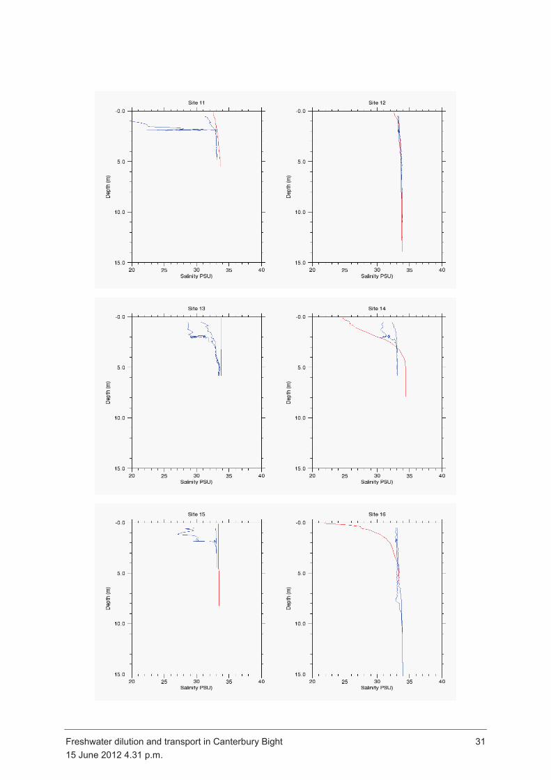
There were two CTD surveys, each comprising 30 casts. The observed salinity profiles have
been collocated with the modelled salinity; figures showing the 60 comparisons are shown in
Appendix B.
Agreement between the observed and modelled salinity is variable. Some profiles (Survey 1,
Site 3) match very well, some (Survey 1, Site 6) do not. In some cases (Survey 1, Site 5) the
model agrees with one cast of the CTD but not with the other. Given that the spacing in time
between the downcast and the upcast is typically 10 minutes, this indicates considerable
short-term variability (and probably considerable small-scale spatial variability) in the
freshwater layer.
The thickness of the observed surface freshwater layer on the inshore transect is typically 2–
5 m and the model generally agrees with this, though the model never develops the very
sharp salinity discontinuities that mark the base of the layer in the CTD casts. On the
offshore transects, the salinity depression is smaller and the thickness of the freshwater
layer, if it is apparent at all, is 5–7 m. Again the model reproduces this behaviour.

Freshwater dilution and transport in Canterbury Bight 17
15 June 2012 4.31 p.m.
Overall the comparison indicates that the model does not match the small-scale variability
that characterises the freshwater layer on the inshore transect, but tends to produce a
freshwater layer with salinity depression and thickness of approximately the correct
magnitude.
5 Results Section 2.3 described a simulation on the inner domain (1 km grid) covering a period of
slightly more than one year in 2009–2010. From this simulation were saved fields of
temperature, salinity, velocity and freshwater dye concentration as averages over
consecutive 12-hour intervals. Possibly the most instructive way to examine model output is
by viewing animated graphs; several of these are included with the electronic version of this
report, as described in Appendix A.
The animated graphs of surface velocity, temperature and salinity show some of the basic
oceanography of the area. The Southland Current is evident as a region of persistent flow
towards the northeast along the shelf break, following the 500 m depth contour (Figure 1c).
On the continental shelf the surface water moves back and forth, mainly in response to
forcing by the wind. Tides are included in this simulation and the 12-hour averaging filters out
most, but not all, of the tidal motion: what remains is largely responsible for the “jittery”
character of the velocity plot. Over periods of a week or more the surface water in
Canterbury Bight generally drifts to the northeast and past Banks Peninsula. Along the coast
of Canterbury Bight there is a band ~10 km wide in which the currents, temperature and
salinity are quite variable, due to the effects of freshwater input from the rivers and also
coastal upwelling and downwelling. The salinity is generally lowest (< 33.5 psu) near the
coast, highest (~34.6 psu) in the subtropical water on the outer shelf and lower again
(~34.3 psu) in the subantarctic water beyond the shelf break.
Animated graphs are also included of the freshwater tracers (Table 1) individually and of their
sum. Looking first at the animation of the surface total freshwater concentration
(dye_01+dye_02+dye_03+dye_04+dye_05+dye_06+dye_07+dye_08.avi):
§ One can see a plume associated with each of the major rivers and a broader
freshwater band attached to the coast.
§ The surface freshwater concentration in the river plumes regularly exceeds 30%
(the scale maximum) within a few kilometres of the source.
§ The river plumes move back and forth, and the width of the coastal freshwater
band fluctuates, on time scales of several days. The animations include a barb
indicating the direction and magnitude of the surface stress. The relationship
between plume behaviour and surface stress is not straightforward, but, broadly
speaking, a stress directed to the S (a northerly wind) spreads the freshwater
band away from the coast, whereas a stress directed to the NE (a south-
westerly wind) produces a narrow freshwater band moving north-eastward
along the coast.

18 Freshwater dilution and transport in Canterbury Bight
The total freshwater concentration at 10 m depth (dye_01+dye_02+dye_03+dye_04+-
dye_05+dye_06+dye_07+dye_08_10.0_m.avi) is much lower than at the surface, indicating
that the plumes are generally shallow features.
In the animations of the individual tracers (dye_01 to dye_08), points to note include:
§ Freshwater from the Southland and Otago rivers (dye_01) is periodically
injected into Canterbury Bight and then tends to persist, at concentrations less
than 1%. On other occasions, one can see pulses of this water moving past
Canterbury Bight in the Southland Current.
§ Waitaki River water (dye_02) forms an extensive plume that tends to move
along the coast towards Timaru or be swept offshore, sometimes being picked
up by the Southland Current and moved rapidly north-eastward.
§ Plumes from the Opihi (dye_03), Rangitata (dye_04) and Ashburton (dye_05)
Rivers move back and forth along the coast of central Canterbury Bight, with
occasional rapid excursions towards Banks Peninsula. These excursions
occurred during the first few months of the one-year simulation period and the
most pronounced one was around 22–26 May 2009.
§ The Rakaia River (dye_06) produced higher surface concentrations around
Banks Peninsula than any other single source. Rakaia River water entered
Pegasus Bay on several occasions, but at surface concentrations of no more
than a few percent.
§ Lake Ellesmere/Te Waihora (dye_08) was open twice during the simulation
period. The plume affected northern Canterbury Bight and southern and eastern
Banks Peninsula.
§ The Waimakariri River (dye_07) plume was normally contained within Pegasus
Bay, more often in the northern part.
Mean and maximum surface freshwater concentrations have been calculated from the tracer
data and are shown in Figure 9 (surface) and Figure 10 (10 m depth). At the surface, the
highest concentrations occur near the mouths of the major rivers (Waitaki, Rangitata, Rakaia
and Waimakariri): the mean concentrations here are in excess of 30% and the maximum
concentrations approach 100%. The lowest concentrations at the Canterbury coastline occur
on northern Banks Peninsula (mean ~3%, maximum ~10%).
At 10 m depth the concentrations are much lower than at the surface and also more evenly
distributed. The mean concentration in Canterbury Bight is typically 1–3% and the maximum
is 2–6%.
Table 2: Sites for vertical profiles. See also Figure 11.
Site Location Description
A 171.209° E, 44.971° S Waitaki River plume, 20 m contour
B 172.225° E, 43.948° S Rakaia River transect, 20 m contour
C 172.317° E, 44.108° S Rakaia River transect, 40 m contour
D 172.544° E, 44.392° S Rakaia River transect, 100 m contour

Freshwater dilution and transport in Canterbury Bight 19
15 June 2012 4.31 p.m.
Site Location Description
E 172.973° E, 43.913° S Near Akaroa Harbour entrance
F 172.836° E, 43.578° S Lyttleton Harbour/Port Levy entrance
To further elucidate the vertical variation in freshwater concentrations, six sites have been
specified (Table 1, Figure 11) and vertical profiles extracted at each one from the 12-hour
average model output. The mean and maximum concentrations at each site are shown in
Figure 12 for the same one-year period as shown in Figure 9 and Figure 10.

20 Freshwater dilution and transport in Canterbury Bight
Figure 9: Mean (upper) and maximum (lower) surface freshwater concentration . Statistics calculated for the sum of the eight freshwater tracers over the 365 day period from 21 April 2009 to 21 April 2010.
Figure 10: Mean (upper) and maximum (lower) freshwater concentration at 10 m depth. Statistics calculated for the sum of the eight freshwater tracers over the 365 day period from 21 April 2009 to 21 April 2010.

Freshwater dilution and transport in Canterbury Bight 21
15 June 2012 4.31 p.m.
Two of the sites (A and B) are within a few kilometres of the largest rivers (Waitaki and
Rakaia, respectively. Maximum concentrations there are 50–70% and mean concentrations
~20%. The concentrations drop off rapidly in the top 3 m of the water column and below 5 m
are always less than 10%. Sites B, C and D form a transect out from the Rakaia River and
Figure 12 clearly shows the drop-off in concentration with distance from the coast and/or
depth. Site E, in relatively deep water at the entrance to Akaroa Harbour shows quite a high
maximum concentration (~35%) associated with shallow plumes from the Rakaia River; Site
F, in much shallower water at the entrance to Lyttleton Harbour and Port Levy, has much
lower concentrations.

22 Freshwater dilution and transport in Canterbury Bight
Figure 11: Sites for vertical profiles. See also Table 2 and Figure 12.

Freshwater dilution and transport in Canterbury Bight 23
15 June 2012 4.31 p.m.
Figure 12: Profiles of mean and maximum freshwater concentration at six sites. See Table 2 and Figure 11.
6 Discussion The model has produced freshwater plumes with behaviour that is physically plausible and
qualitatively consistent with remote sensing results (Schwarz 2008,Schwarz et al. 2010).
The model verification confirms that the model is simulating currents in the area very well
and that the behaviour of the surface freshwater layer is realistic, though it does not
reproduce the small-scale variability on the in-shore transect during the CTD surveys in July
and December 2011. Plumes are initially confined very close to the surface (typically 1–3 m)
and have freshwater concentrations of 10–30%, frequently more and occasionally
approaching 100%. Such concentrated plumes can often be detected several kilometres
from the source. The plumes are progressively diluted by vertical mixing and horizontal
dispersion, forming a coastal band ~10 km wide with surface freshwater concentrations
typically 5–10%. Further out in Canterbury Bight the surface freshwater concentrations are
lower still (1–5%) and include a significant contribution from Southland and Otago rivers,
notably the Clutha River.
The coastal freshwater band, and the river plumes within it, are transported by surface
currents, which produce a general north-eastward drift but with fluctuations that are largely
wind driven. When the wind is from the south or southwest, the coastal freshwater band
becomes narrower and can move quite quickly (within a few days) north-eastward along the
coast of Canterbury Bight and around the end of Banks Peninsula.
The model indicates substantially higher freshwater concentrations on the southern and
eastern sides of Banks Peninsula than on the northern side (e.g. see Figure 9 and Figure
12). The concentrations on the northern side are relatively low because freshwater from
rivers to the south (notably the Rakaia) tend to be diluted as they enter Pegasus Bay, while
the Waimakariri plume tends to move northward and does not produce high concentrations
adjacent to Banks Peninsula. Note that this finding depends on the model’s representation of
the circulation in Pegasus Bay, and there are not sufficient data to confirm that this
representation is essentially correct.

24 Freshwater dilution and transport in Canterbury Bight
7 Acknowledgements River flow data were provided by Kathy Walter of NIWA and originated from Environment
Southland, Otago Regional Council, Environment Canterbury and NIWA archives.
The field measurement programme was conducted by Warren Thompson of NIWA, who
worked long hours to ensure high-quality data.
Thanks to Lesley Bolton-Ritchie of Environment Canterbury for her feedback on a preliminary
version of the report.

26 Freshwater dilution and transport in Canterbury Bight
8 Glossary of abbreviations and terms
climatological In connection with model forcing, an adjective describing data (frequently
at one-month intervals) with an annual cycle that is repeated indefinitely,
thus representing generic conditions, cf. real-time.
real-time In connection with model forcing, an adjective describing a dataset
representing a sequence of actual dates and times, cf. climatological.

26 Freshwater dilution and transport in Canterbury Bight
9 References Carton, J.A.; Giese, B.S. (2008). A reanalysis of ocean climate using simple ocean
data assimilation (SODA). Monthly Weather Review 136(8): 2999–3017.
doi:10.1175/2007MWR1978.1
Chiswell, S.M. (1996). Variability in the Southland Current, New Zealand. New
Zealand Journal of Marine and Freshwater Research 30(1): 1–17.
doi:10.1080/00288330.1996.9516693
Haidvogel, D.B.; Arango, H.; Budgell, W.P.; Cornuelle, B.D.; Curchitser, E.; Di
Lorenzo, E.; Fennel, K.; Geyer, W.R.; Hermann, A.J.; Lanerolle, L.; Levin, J.;
McWilliams, J.C.; Miller, A.J.; Moore, A.M.; Powell, T.M.; Shchepetkin, A.F.;
Sherwood, C.R.; Signell, R.P.; Warner, J.C.; Wilkin, J. (2008). Ocean forecasting
in terrain-following coordinates: Formulation and skill assessment of the Regional
Ocean Modeling System. Journal of Computational Physics 227(7): 3595–3624.
doi:10.1016/j.jcp.2007.06.016.
Horrell, G.A. (2009). Lake Ellesmere (Te Waihora) water balance model: variable
update 1991 to 2007. NIWA Client Report CHC2009-102. 35 p.
Kalnay, E.; Kanamitsu, M.; Kistler, R.; Collins, W.; Deaven, D.; Gandin, L.; Iredell,
M.; Saha, S.; White, G.; Woollen, J.; Zhu, Y.; Leetmaa, A.; Reynolds, R.W.;
Chelliah, M.; Ebisuzaki, W.; Higgins, W.; Janowiak, J.; Mo, K.C.; Ropelewski, C.;
Wang, J.; Jenne, R.; Joseph, D. (1996). The NCEP/NCAR 40-Year Reanalysis
Project. Bulletin of the American Meteorological Society 77(3): 437–471.
doi:10.1175/1520-0477(1996)077<0437:TNYRP>2.0.CO;2
MacCready, P.; Banas, N.S.; Hickey, B.M.; Dever, E.P.; Liu, Y. (2009). A model
study of tide- and wind-induced mixing in the Columbia River Estuary and plume.
Continental Shelf Research 29(1): 278–291. doi:10.1029/2004JC002691
Rickard, G.J.; Hadfield, M.G.; Roberts, M.J. (2005). Development of a regional
ocean model for New Zealand. New Zealand Journal of Marine and Freshwater
Research 39(5): 11711191. doi:10.1080/00288330.2005.9517383
Reynolds, R.W.; Rayner, N.A.; Smith, T.M.; Stokes, D.C.; Wang, W. (2002). An
improved in situ and satellite SST analysis for climate. Journal of Climate 15(13):
1609–1625. doi:10.1175/1520-0442(2002)015<1609:AIISAS>2.0.CO;2
Schwarz, J.N. (2008). Remote sensing of river plumes in the Canterbury Bight:
Stage I report. NIWA Client Report: CHC2008-169. 68 p.
Schwarz, J.N.; Pinkerton, M.H.; Wood, S.; Zeldis, J.R. (2010). Remote sensing of
river plumes in the Canterbury Bight Stage II: Final Report. NIWA Client Report:
CHC2010-048. 180 p.
Smith, S.D. (1988). Coefficients for sea surface wind stress, heat flux, and wind
profiles as a function of wind speed and temperature. Journal of Geophysical
Research 93(C12): 15467–15472.

Freshwater dilution and transport in Canterbury Bight 27
15 June 2012 4.31 p.m.
Stanton, B.R.; Goring, D.G.; Bell, R.G. (2001). Observed and modelled tidal currents
in the New Zealand region. New Zealand Journal of Marine and Freshwater
Research 35(2): 397–415. doi:10.1080/00288330.2001.9517010
Sutton, P.J.H. (2003). The Southland Current: a subantarctic current. New Zealand
Journal of Marine and Freshwater Research 37(3): 645–652.
doi:10.1080/00288330.2003.9517195
Thompson, R.O.R.Y. (1983). Low-pass filters to suppress inertial and tidal
frequencies. Journal of Physical Oceanography 13(6): 1077–1083.
Walters, R.A.; Goring, D.G.; Bell, R.G. (2001). Ocean tides around New Zealand.
New Zealand Journal of Marine and Freshwater Research 35(3): 567–579.
doi:10.1080/00288330.2001.9517023

28 Freshwater dilution and transport in Canterbury Bight
Appendix A Animations Several animations of model output are included with the electronic version of the report in a
subdirectory called Animations. On Windows we recommend that you view them with a free
media player called Imagen, available from the following Web page:
http://gromada.com/imagen/
Otherwise you can use Windows Media Player or QuickTime Player. The advantage of
Imagen is that it allows fast & easy navigation, either forward or backward, through the
animation with the computer’s keyboard. (Use the space bar to pause or restart the
animation, left and right arrow keys to step one frame, and the Home and End keys to move
to the beginning and end of the animation.)
The Animations subdirectory includes an HTML document (index.html) with links to the
animations, along with a brief description of each one. If the location of the Animations
subdirectory relative to this report has been preserved, you should be able to open the
index.html using the following relative link:
Animations/index.html
Alternatively, you can navigate to the Animations subdirectory and open index.html in a Web
browser directly.

Freshwater dilution and transport in Canterbury Bight 29
15 June 2012 4.31 p.m.
Appendix B CTD-model comparisons Survey 1 (4 July 2011), near-shore transect (Sites 1 to 25)

30 Freshwater dilution and transport in Canterbury Bight
Freshwater dilution and transport in Canterbury Bight 31
15 June 2012 4.31 p.m.

32 Freshwater dilution and transport in Canterbury Bight

Freshwater dilution and transport in Canterbury Bight 33
15 June 2012 4.31 p.m.
Survey 1 (4 July 2011), off-shore transect (Sites 26 to 30)

34 Freshwater dilution and transport in Canterbury Bight
Survey 2 (9 December 2011), near-shore transect (Sites 1 to 25)

Freshwater dilution and transport in Canterbury Bight 35
15 June 2012 4.31 p.m.

36 Freshwater dilution and transport in Canterbury Bight

Freshwater dilution and transport in Canterbury Bight 37
15 June 2012 4.31 p.m.

38 Freshwater dilution and transport in Canterbury Bight

Freshwater dilution and transport in Canterbury Bight 39
15 June 2012 4.31 p.m.
Survey 2 (9 December 2011), off-shore transect (Sites 26 to 30)