PREFERENCE UNCERTAINTY IN NON-MARKET VALUATION:

A FUZZY APPROACH

by

G. Cornelis van Kooten, Department of Economics, University of Victoria, Victoria, Canada

Emina Krcmar

FEPA Research Unit, University of British Columbia, Vancouver, Canada

and

Erwin H. Bulte, Department of Economics, Tilburg University, Netherlands

Abstract

In this paper, we consider uncertain preferences for non-market goods, but we move away from a probabilistic representation of uncertainty and propose the use of fuzzy contingent valuation (CV). We assume that a decision maker never fully knows her own utility function and we treat utility as a fuzzy number. The methodology is illustrated using data on forest valuation in Sweden. Fuzzy CV provides estimates of resource value in the form of a fuzzy number and includes estimates obtained using a standard probabilistic approach.

Key Words: Fuzzy set theory; fuzzy contingent valuation; forest preservation; preference uncertainty Acknowledgements: The authors wish to thank Chuan–Zhong Li and Leif Mattsson for graciously sharing their data. They also wish to thank the Sustainable Forest Management Network at the University of Alberta and the Agricultural Economics and Rural Policy Group at the University of Wageningen for research support.

PREFERENCE UNCERTAINTY IN NON-MARKET VALUATION: A FUZZY APPROACH

1. Introduction

The contingent valuation (CV) survey method is a widely used technique for valuing

non-market environmental amenities. In forestry, for example, both commercial timber

values and non-timber values are important for guiding policy. Commercial timber values

are straightforward to measure using market data and the travel cost method can be used

to find forest recreation benefits, but CV is generally required to provide estimates of

preservation value, which may be the most important non-timber value.

Most CV surveys rely on a dichotomous choice question to elicit either

willingness to pay (WTP) or compensation demanded. Calculation of the Hicksian

compensating or equivalent welfare measure is based on the assumption that the survey

respondent knows her utility function with certainty (Hanemann 1984; Hanemann and

Kriström 1995). This assumption implies that the respondent knows with certainty how

much she would be willing to pay for the good in question.

The assumption of preference certainty is a strong one because CV seeks to elicit

values for environmental resources from respondents who may lack the cognitive ability

to make such assessments (Gregory et al. 1993; Sagoff 1994; Knetsch 2000). While

Hanemann and Kriström (1995) provide an explanation of what preference uncertainty

means in the context of the CV method, several authors have adopted varying but ad hoc

approaches for dealing with preference uncertainty in non-market valuation (Ready et al.

1995; Loomis and Ekstrand 1998). These approaches rely on probabilistic interpretations

of uncertainty. Our contention is that the apparent precision of standard WTP estimates

2

(even as a mean value with confidence interval) masks the underlying vagueness of

preferences and may lead to biased outcomes (Barrett and Pattanaik 1989).

Fuzzy set theory (Zadeh 1965) provides a useful alternative for interpreting

preference uncertainty and analyzing willingness to pay responses in the CV framework.

Fuzzy logic addresses both imprecision about what is to be valued (Li 1989; Treadwell

1995) and uncertainty about values that are actually measured (Cox 1994). In this paper,

we focus on the most often used economic application of fuzzy set theory––modelling of

choices based on vague preferences (Basu 1984; Barrett and Pattanaik 1989; Barrett et al.

1990; Banerjee 1995). We distinguish between three types of uncertainty that could cause

ill-defined preferences for environmental goods.

First, people may not be well acquainted with the alternatives they are being

asked to value, and cannot easily express a preference for different combinations of

income and the environmental amenity. For example, a survey of Scottish citizens

revealed that over 70% of the respondents were completely unfamiliar with the meaning

of biodiversity (Hanley et al. 1997). Similarly, some respondents are likely not familiar

with ‘obscure’ endangered species such as the striped shiner or the squawfish, yet are

asked to value their survival (Bulte and van Kooten 1999). One straightforward means for

mitigating this type of uncertainty is to provide more information or detail about the

amenity to be valued.

Second, respondents may be truly uncertain about their preferences because they

have never previously given such tradeoffs much thought. In a one-shot CV experiment,

a respondent’s stated WTP may be biased. One approach in this case is to use focus

groups that enable stakeholders (as opposed to a truly representative group) to construct a

3

preference function (McDaniels 1996). Other approaches have also been proposed to

address this type of uncertainty, all relying on a probabilistic interpretation of uncertainty

(Kriström 1997; Loomis and Edstrand 1998).

Third, and crucial for the current paper, it may be the case that respondents never

fully know their preferences. The concern here is with a respondent’s cognitive inability

to rank commodities with diverse properties, even if the commodities themselves are well

defined and their attributes completely known by the respondent (Fedrizzi 1987; Irwin et

al. 1993). So far, this type of uncertainty has been ignored in much of the economic

valuation literature, and certainly in the valuation of non-market goods.

There is a fundamental and philosophical difference between the second and third

approaches to uncertain preferences. The second approach assumes that respondents learn

about their preferences over time (Hoehn and Randall 1987) and eventually ‘know’ their

true utility function. In other words, respondents are uncertain about the location of their

true indifference curve(s), but a time series of CV surveying would measure a shifting

‘perceived’ indifference curve that gradually approaches the true one. The third approach,

in contrast, treats the utility function as a useful analytical construct, but acknowledges

that certain trade-offs are inherently difficult, if not impossible, to make. How does one

value ‘employment’ versus ‘endangered species conservation,’ or ‘children’s health’

versus ‘poverty alleviation’? While respondents will certainly have some preference over

such choices, valuation at the margin is extremely difficult and it is obvious that some

trade-offs cannot be represented by a true and unique indifference curve. In this paper, we

replace this notion with that of a fuzzy set. Li and Mattsson (1995) were among the first

to incorporate preference uncertainty (of the second type) into a discrete choice model of

4

WTP. They assumed that each individual has a true value for the amenity in question, but

that the respondent does not yet know that value with certainty. They then develop a CV

survey that uses a post–decisional confidence measure on each respondent’s ‘yes/no’

answer about willingness to pay a given ‘bid’ for the amenity. They integrate this

confidence measure into the standard dichotomous-choice WTP model. Li and Mattsson

model the respondent’s ‘yes/no’ choice as a realization of some probabilistic mechanism

where the post-decisional confidence is interpreted as a subjective probability that the

change in the respondent’s utility is positive (for a ‘yes’ answer) or negative (for a ‘no’

answer). In contrast to this approach, we assume that an individual does not have an exact

value for amenity and will therefore never know it with certainty. We assume only that a

respondent knows the level above which she certainly rejects to pay the bid amount for

the amenity and the level below which she certainly accepts the bid. In between these

levels, the preferences of the respondent are vague. In what follows, we use Li and

Mattsson’s data on Swedish forest preservation to illustrate how preference uncertainty of

the third kind can be addressed using fuzzy set theory.

The paper is organized as follows. In section 2, we present a background to fuzzy

logic, focusing on means for comparing fuzzy numbers. Then, in section 3, we briefly

review the traditional contingent valuation method indicating, in section 4, how our fuzzy

approach modifies it. We then, in section 5, apply our approach to a case study of forest

preservation in Sweden, comparing the results with those using traditional valuation

methods. Our conclusions follow.

5

2. Background to Fuzzy Logic

Multivalued logic was first introduced in the 1920s to address indeterminacy in quantum

theory. This was done by permitting a third, or intermediate, possibility in the traditional

bivalent logical framework. The Polish mathematician Jan Lukasiewicz introduced three–

valued logic and then extended the range of truth values from {0, 1/2, 1} to all rational

numbers in [0, 1] and finally to all numbers in [0, 1]. In the late 1930s, quantum

philosopher Max Black used the term ‘vagueness’ to refer to Lukasiewicz’ uncertainty

and introduced the idea of a membership function (Kosko 1992, pp.5-6). Subsequently,

Lofti Zadeh (1965) introduced the term fuzzy set and the fuzzy logic it supports.

Zadeh’s concern was with the ambiguity and vagueness of natural language, and

the attendant inability to convey crisp information linguistically. The subjective

perception of heat by one person is not necessarily congruent with the perception of heat

by another person. There is no absolute temperature at which a thing may be said to

belong in the set of things that are ‘hot,’ or at which it has ceased to be merely ‘warm.’

Subjective interpretations of the term allow for an overlap of temperature ranges. Thus,

an object is said to be ‘warm’ by some while it is judged ‘hot’ by others. In essence, it is

accorded partial membership in both of the sets—it displays some of the requirements for

‘hot’ while retaining some of the requirements for being ‘warm.’ It is this concept of

partial membership that is central to the theory of fuzzy sets. In what follows, we apply

the same reasoning to analyze vague preferences rather than vague language (see also

Ells et al. 1997). Thus, a bid may be fully acceptable or fully unacceptable to a

respondent (i.e., full membership in the set of acceptable and unacceptable bids,

respectively), but it may also be a bit of both.

6

Consider the idea of partial membership more formally. An element x of the

universal set X is assigned to an ordinary (crisp) set A via the characteristic function µA,

such that:

µA(x) = 1 if x∈A.

(1)

µA(x) = 0 otherwise. The element has either full membership (µA(x)=1) or no membership (µA(x)=0) in the set

A. A fuzzy set A~ is also described by a characteristic function, the difference being that

the function now maps over the closed interval [0,1]. Thus, an element may be assigned a

value that lies between 0 and 1 and is representative of the degree of membership that x

has in the fuzzy set A~ .1 A membership function describes the relative grade or degree of

membership, with the membership function viewed as a representation of a fuzzy number

(Klir and Folger 1988, p.17).

Zadeh (1965) originally proposed operations for fuzzy sets, defining the

intersection of two fuzzy sets A~ and B~ as:

(2) Xxxxx BABA ∈∀=∩

)},(),(min{)( ~~~~ µµµ ,

and union as:

(3) Xxxxx BABA ∈∀=∪

)},(),(max{)( ~~~~ µµµ .

Intersection A~ ∩ is the largest fuzzy set that is contained in both B~ A~ and , and union B~

A~ ∪ is the smallest fuzzy set containing both B~ A~ and . Both union and intersection of

fuzzy sets are commutative, associate and distributive as for crisp (ordinary) sets. Further,

B~

1By convention, membership functions are normalized so that there exists at least one x∈X such that A~µ (x) = 1, and 0 ≤ A~µ (x) ≤ 1 ∀ x∈X.

7

the complement A~ c of fuzzy set A~ is defined as:

A~

µ

(4) µ (x) = 1 – µ (x). CA~ A~

Fuzzy logic deviates from crisp or bivalent logic because, if we do not know A~

with certainty, its complement C is also not known with certainty. Thus, A~ C ∩ A~ does

not necessarily produce the empty set as is the case for crisp sets (where AC ∩ A = φ).

Fuzzy logic violates the “law of noncontradiction” and the “law of the excluded middle,”

because the union of a fuzzy set and its complement does not equal the universe of

discourse (the universal set).

Finally, we define the α-level set, Aα, as that subset of values of A~ for which the

degree of membership exceeds the level α

(5) Aα = { x | A~ (x) ≥α}, α∈(0,1].

The result Aα is itself crisp.

Fuzzy numbers and fuzzy arithmetic

In this paper, we express uncertainty in terms of fuzzy numbers. A fuzzy number F~ is a

fuzzy set defined on the real line with the membership function µ (x) ∈ [0,1]. Fuzzy sets

can be used to express concepts of approximate functions and numbers (e.g., ‘closeness’

or ‘nearness’ to a function or number, as well as linguistic concepts like ‘large’ or

‘small’). Both interpretations are useful in the context of CV, but here we focus on

approximation. As an example, a non-symmetric, triangular fuzzy number

F~

F~ =(f, d1, d2)

with center f, left spread d1 and right spread d2 is presented in Figure 1. It has the

membership function:

8

1 – 1d

xf − , f – d1 ≤ x ≤ f

(6) F~µ (x) = 1 – 2d

fx − , f ≤ x ≤ f+d2

0, otherwise.

<INSERT FIGURE 1 ABOUT HERE>

Alternative specifications of membership functions are possible. If the left spread

approaches infinity, the resulting fuzzy number becomes M~ =(f, ∞, d2), which has the

membership function:

1, x ≤ f

(7) )(~ xMµ = 1 – 2dfx − , f ≤ x ≤ f+d2

0, otherwise Such a number may describe respondents’ WTPs for a certain environmental amenity; it

may describe the fuzzy set of ‘bids that are acceptable to respondents.’ Respondents are

always willing to pay an amount less than f (with membership in fuzzy WTP equal to

one), but membership decreases as the bid increases beyond f and eventually falls to zero.

If the right spread of a fuzzy number approaches infinity, or N~ =(g, d1, ∞), it has

membership function:

1, x ≥ g

(8) N~µ (x) = 1 – 1dxg − , g– d1 ≤ x ≤ g

0, otherwise. Numbers of this type could represent respondents’ willingness not to pay (WNTP) for an

environmental amenity. Thus, it may be used to define the fuzzy set ‘bids that are

unacceptable to respondents.’ Further, membership functions need not be (piecewise)

9

linear, but can be highly nonlinear (see below).

Operations on fuzzy numbers are the extension of operations on real numbers

(Kauffman and Gupta 1985; Kosko 1992; Klir and Yuan 1995). For fuzzy sets F~ and G~ ,

x, y, z∈ℜ, addition and subtraction can be defined as:

(9) )](),(min[sup)( ~~~~ yxz GFyxz

GF µµµ+=

+=

(10) )](),(min[sup)( ~~~~ yxz GFyxz

GF µµµ−=

−=

Comparing fuzzy numbers

For any two crisp numbers F and G, only one of the relations F<G, F>G or F=G holds.

For two fuzzy numbers F~ and G~ , two ordering relations can hold simultaneously. The

order of fuzzy numbers cannot be established in an absolute sense, but only to a degree.

Comparison of fuzzy numbers has received significant attention in connection with

special types of decision problems (see Chen and Hwang 1992; Munda et al.1995). The

ordering of fuzzy numbers represents a relation of partial order and thus involves the

notion of preference rather than ‘greater than.’ Three classes of methods for ordering

fuzzy numbers have been proposed. First are the methods that extend preference between

crisp numbers to fuzzy numbers. The second includes approaches that rely on intuition to

determine which of two fuzzy numbers is preferred over the other. While the first

addresses the order of fuzzy numbers along the horizontal axis (the values of fuzzy

numbers), the second relies on membership values (the vertical component of a fuzzy

number). Both approaches have disadvantages since they limit comparison to only one

aspect (component) of the fuzzy number. Different approaches in ordering fuzzy numbers

10

are illustrated using the two fuzzy numbers in Figure 2.

<INSERT FIGURE 2 ABOUT HERE>

In Figure 2, the order of fuzzy numbers F~ and G~ along the horizontal axis is

based on the partial order of the closed intervals (Klir and Yuan 1995, p.114). Let f~

denote the fuzzy relation ‘greater than or equal to.’ Then

(11) F~ f~ G~ if and only if [f1, f2] ≥ [g1,g2] if and only if f1 ≥ g1 and f2 ≥ g2 .

If membership values are taken into account, the partial order of fuzzy numbers

can be defined in terms of their α–cuts (vertical component). For fuzzy numbers F~ and

G~ , α–cuts Fα and Gα are closed intervals. The fuzzy relation F~ f~ G~ is then defined as

(Klir and Yuan 1995, p.114):

(12) F~ f~ G~ if and only if Fα ≥Gα for all α∈(0,1].

When this definition is applied to the fuzzy numbers in Figure 2, different orderings of

F~ and are obtained at various α-levels. First, G~ F~ f~ G~ for α∈(0, α1]. For α∈(α1,α2),

the fuzzy numbers F~ and are not comparable. Finally, G~ F~ p~ G~ for α∈(α2, 1].

Inconsistencies in ordering fuzzy numbers for different approaches and even for

the same definition motivate the third approach. In situations of overlap (as in Figure 2),

methods based on area measurement are generally able to order fuzzy numbers where

other methods fail to establish an order. Yager (1981) was among the first to compare

fuzzy numbers in terms of area measurement by introducing a ranking index for a fuzzy

number. Several criteria for choosing between two fuzzy numbers based on the Hamming

11

distance or its variations have been proposed (Kauffman and Gupta 1985; Saade and

Schwarzlander 1992).

Ordering of fuzzy numbers usually establishes a binary relation between fuzzy

numbers. Based on the area measurement approach, we introduce the notion of the

strength (degree) of the relation between two fuzzy numbers. We define the fuzzy

relation between two fuzzy numbers in terms of the areas under the membership

functions, S1, S2, S3, S4 and S5 in Figure 2. Let s∈[0,1] denote the normalized strength of

the fuzzy relations ‘greater than or equal to’ ( ) and ‘less than or equal to’ ( ). The

strength of

f~ p~

F~ p~ G~ is represented by the sum of areas S2, S3 and S5. Similarly, the

strength of F~ f~ G~ is defined by S1+S4+S5. The strength of a relation between two fuzzy

numbers is normalized by dividing by S=S1+S2+S3+S4+S5, or the total area under the

membership curves for F~ and . G~

Let F be the set of fuzzy numbers. We can define fuzzy orderings as follows:

Definition 1. (Fuzzy less than or equal to). For given F~ , ∈F,

s(

G~

F~ p~ G~ )=(S2+S3+S5)/S.

Definition 2. (Fuzzy greater than or equal). For given F~ , ∈F,

s(

G~

F~ f~ G~ )=(S1+S4+S5)/S.

Notice that s( F~ p~ G~ )+s( F~ f~ G~ )≥1. This results follows because fuzzy logic violates the

“law of the excluded middle” (Barrett and Pattanaik 1989).

12

The application of Definitions 1 and 2 for comparing two fuzzy numbers, F~ and

, is illustrated in Figure 3. In panel 3(a), s(G~ F~ p~ G~ )=1 since (S2+S3+S5)/S=1. Likewise,

s( F~ f~ G~ )=0 as S1+S4+S5=0. As G approaches ~ F~ , the area of overlap between the

membership functions increases. Then, s( F~ p~ G~ ) remains 1 and s( F~ f~ G~ ) increases. As

long as S1 and S4 are zero, S=S2+S3+S5, s( F~ p~ G~ )=1 and s( F~ f~ G~ )=S5/S (Figure 3b).

Panel 3(c) illustrates a case of non-obvious relations between two fuzzy numbers. Both

relations and hold simultaneously to some degree. p~ f~

<INSERT FIGURE 3 ABOUT HERE>

In Figure 3, situations (a) and (b) differ only by the overlap area between the

membership functions. To distinguish between these cases, we introduce the relation

‘fuzzy overlap’ (denoted by ~). The normalized strength of s( F~ ~ ) is defined as: G~

Definition 3. (Fuzzy overlap ~). From Figure 3, for given F~ , ∈F,

s(

G~

F~ ~G )=S5/S. ~

Fuzzy Preference

If F is a set of fuzzy numbers, a fuzzy preference relation is a function ρ:F ×F→[0,1].

We interpret ρ( F~ , ) as the degree to which G~ F~ is preferred to or the degree to

which ‘

G~

F~ is at least as good as ’ (Barrett and Pattanaik 1989). G~

13

Definition 4. (Fuzzy preference) For given F~ , ∈F, G~ F~ is preferred to G if and only

if s(

~

F~ f~ G~ )≥s( F~ p~ G~ ). Then, ρ( F~ , )=s(G~ F~ f~ G~ ).

It may be easily proved that a fuzzy preference relation between F~ and (Definition 4)

is reflexive, connected and transitive in terms of the following axioms:

G~

Reflexivity. ρ( F~ , F~ ) =1, ∀ F~ ∈F .

Connectedness. ρ( F~ , )+ρ(G ,G~ ~ F~ )≥1 ∀ F~ , G ∈F . ~

Max-min Transitivity. ρ( F~ , H~ )≥min[ρ( F~ ,G ), ρ( ,~ G~ H~ )] ∀ F~ , G ,~ H~ ∈F .

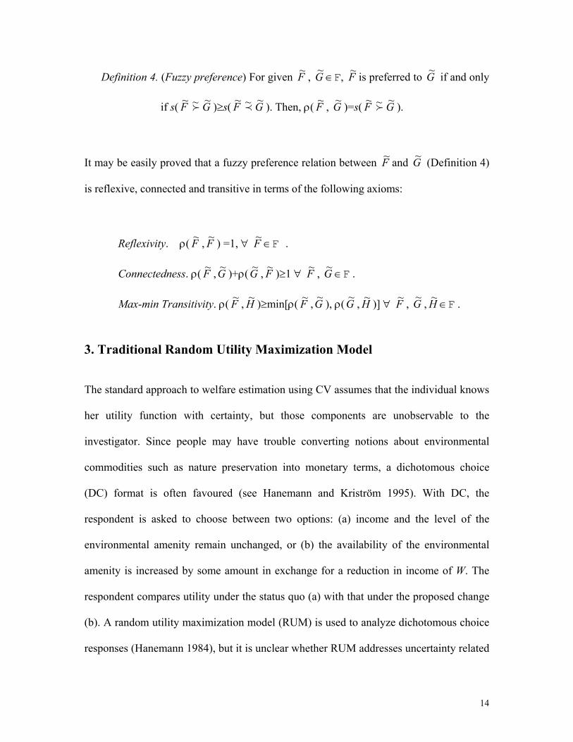
3. Traditional Random Utility Maximization Model

The standard approach to welfare estimation using CV assumes that the individual knows

her utility function with certainty, but those components are unobservable to the

investigator. Since people may have trouble converting notions about environmental

commodities such as nature preservation into monetary terms, a dichotomous choice

(DC) format is often favoured (see Hanemann and Kriström 1995). With DC, the

respondent is asked to choose between two options: (a) income and the level of the

environmental amenity remain unchanged, or (b) the availability of the environmental

amenity is increased by some amount in exchange for a reduction in income of W. The

respondent compares utility under the status quo (a) with that under the proposed change

(b). A random utility maximization model (RUM) is used to analyze dichotomous choice

responses (Hanemann 1984), but it is unclear whether RUM addresses uncertainty related

14

to observation or actual preference uncertainty, or both.

Formally, let u(j, m; r) be a crisp utility function where j∈{0,1} is an indicator

variable that takes on the value 1 if the individual accepts the opportunity to pay the bid

amount W for the amenity and 0 if not, m is income, and r is a vector of the respondent

attributes. If we assume that the respondent knows her utility function with certainty, then

she should be willing to pay amount W as long as

(13) u(1, m–W; r) ≥ u(0, m; r).

In this model, if utility is crisp, there exists a maximum willingness to pay, M, such that

u(1, m–M; r)–u(0, m; r)=0. M is the reduction in income that would make the respondent

indifferent between the status quo (j=0) and the contingency (j=1); it is the Hicksian

compensating surplus.

Consider the simplest case where the utility function has a linear form:

(14) u(j, m; r) = αj + δm + εj with δ>0, j = 0,1,

where αj and δ are parameters of the utility function and εj is an error term associated

with observed uncertainty of the respondent’s utility function. The change in utility

between the two states is then given as:

(15) ∆v = [α1+δ(m–W)+ε1] – [α0+δm+ε0] = (α1–α0)– δW+(ε1–ε0) = α–δW+ε,

where α≡α1–α0 and ε≡ε1–ε0 is iid because εj (j=0,1) are each iid (Hanemann 1984). The

respondent accepts the bid if ∆v>ε0–ε1.

In the classical CV model, ∆v is assumed to be a random variable. If both the

analyst’s uncertainty about the respondent’s utility and the respondent’s uncertainty about

her preferences are assumed to be random, this implies that acquiring additional

15

information can reduce both uncertainties.2 In a case of perfect information then,

uncertainty would be zero. The fuzzy approach to contingent valuation described below

is different because it retains uncertainty even when information is perfect. Thus, the

fuzzy approach should not be regarded as competing with, but rather as complementing,

the standard approaches to preference uncertainty within a CV framework.

4. Fuzzy Utility Functions and Fuzzy Contingent Valuation

Our concern is with people who may have conflicting impulses about which goods they

prefer; they may think that one good is better than another in some respect but worse in

others. We consider respondents’ cognitive (in)ability to rank commodities with diverse

properties, even if the commodities themselves are well defined or crisp, and information

is perfect. An assumption of the DC approach in the CV context is that each respondent is

able to determine which option is preferred, but there are situations when it may be

difficult or impossible for the respondent to determine with certainty the preferred option.

Authors who studied preference uncertainty in the CV framework (Ready et al.

1995; Li and Mattsson 1995; Loomis and Ekstrand 1998) interpret respondents’ difficulty

in making a choice as uncertainty over the location of the indifference curve. Most CV

studies assume that the respondent resolves such uncertainty through additional

information about the amenity being valued. While additional information and

knowledge of the amenity in question may narrow the preference uncertainty region,

preference uncertainty remains as a result of strong conflicts between the objectives

2This assumes that all respondents have the same utility function, a crucial but generally unstated assumption in the random utility maximization model.

16

(Ready et al. 1995). In such situations, a respondent typically adopts one of a variety of

decision rules in order to provide a crisp answer to the DC question. Loomis and

Ekstrand (1998) provide a review and comparison of alternative approaches to

incorporating preference uncertainty into dichotomous choice CV. The methods range

from coding uncertain ‘yes’ responses as ‘no’ (or vice versa) to incorporating a measure

of uncertainty of a DC answer directly into the likelihood function. Despite differences in

the approaches, they are all based on Hanemann’s formulation of the utility difference

model. The underlying assumption of this model and its modifications is that uncertainty

in the model (respondent’s and/or observer’s) can and should be modelled

probabilistically.

Unlike these approaches, we assume that a respondent’s utility is vague and can

be represented by a fuzzy number . Then, the indifference curve is fuzzy too. Graphical

illustration of the DC model when utility is fuzzy is given in Figure 4.3 Income and the

amount of the environmental amenity are assumed to be well defined or crisp.

Representative fuzzy indifference curves are provided in Figure 4 for two individuals (A

and B) faced with the opportunity of paying an amount W to increase the availability of

the environmental amenity from E0 to E1, or remaining at the status quo level K.

Combinations of income and the environmental amenity located on the dark lines have

memberships equal to 1.0 in the fuzzy utility sets, u (A) and (B). Points located off the

dark lines but in the respective shaded areas have a degree of membership in the fuzzy

indifference level that is less than 1.0 but greater than 0. The outside boundaries of the

indifference curve are given by dashed lines. For the respondent with fuzzy indifference

u~

~ u~

3For convenience, the convex indifference curves are drawn as straight lines. See Hanemann and Kriström (1995) for a crisp representation.

17

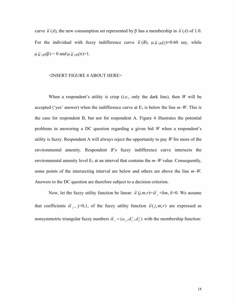
curve (A), the new consumption set represented by β has a membership in u (A) of 1.0.

For the individual with fuzzy indifference curve u (B), µu (B)(γ)=0.60 say, while

µ (B)(β) = 0 and µ (B)(π)=1.

u~ ~

~ ~

j

u~ u~

α~

jα~ ,mj

)2jd

<INSERT FIGURE 4 ABOUT HERE>

When a respondent’s utility is crisp (i.e., only the dark line), then W will be

accepted (‘yes’ answer) when the indifference curve at E1 is below the line m–W. This is

the case for respondent B, but not for respondent A. Figure 4 illustrates the potential

problems in answering a DC question regarding a given bid W when a respondent’s

utility is fuzzy. Respondent A will always reject the opportunity to pay W for more of the

environmental amenity. Respondent B’s fuzzy indifference curve intersects the

environmental amenity level E1 at an interval that contains the m–W value. Consequently,

some points of the intersecting interval are below and others are above the line m–W.

Answers to the DC question are therefore subject to a decision criterion.

Now, let the fuzzy utility function be linear: u (j,m;r)=~ +δm, δ>0. We assume

that coefficients , j=0,1, of the fuzzy utility function );(~ ru are expressed as

nonsymmetric triangular fuzzy numbers ,,(~1j

jj da=α with the membership function:

18

=)(~ xjαµ j

jjj

j axdad

xa≤≤−

−− 1

1

,1

(16) =)(~ xjαµ j

jjjj daxa

dax

22

, +≤<−

−1

=)(~ xjαµ 0, otherwise.

Then, 01~~);,0(~);,1(~~ αδα −−=−−=∆ WrmurWmuv .

A response to the DC question depends on the preference relation ρ( 1~α –δW, 0

~α )

between 1~α –δW and 0

~α . Following Definition 4 (fuzzy preference), a 1~α –δW for a bid W

is preferred to 0~α if and only if s( 1

~α –δWf~ 0~α )≥s( 1

~α –δW p~ 0~α ). The degree to which

1~α –δW is preferred to 0

~α is ρ( 1~α –δW, 0

~α )=s( 1~α –δWf~ 0

~α ).

Choice Rules

The requirement of the DC method is that a respondent provides a clear choice between

the ‘yes’ or ‘no’ answer, even when her preferences are uncertain. Our analysis about

how this choice is made is motivated by the explicit treatment of a respondent’s

preference uncertainty as proposed by Li and Mattsson (1995). Following a standard

contingent valuation question regarding WTP for forest preservation, Li and Mattsson

elicited post-decisional confidence by asking, “How certain were you of your answer to

the previous [dichotomous choice] question?” (p.264). The authors interpreted responses

as the subjective probabilities that the individual’s true valuation is greater (for a ‘yes’

answer) or less (for a ‘no’ answer) than the bid. Li and Mattsson also assume that an

individual may give different ‘yes/no’ answers to the same bid because of the

randomness of her preferences.

19

The format of the confidence question posed by Li and Mattsson allows for different

interpretations. It is known that people have problems interpreting measures of

uncertainty even when these are defined as probabilities. We assume that an individual

always provides the same ‘yes/no’ answer whenever the same bid is offered. Along with

the ‘yes/no’ answer, she provides a number between 0 and 1 that we interpret as a

measure of her comfort, enthusiasm or inclination toward the given answer, or the degree

of membership of the bid in the fuzzy sets of ‘acceptable bids’ and ‘unacceptable bids,’

respectively. As we have seen in section 3, classical CV requires only one value,

maximum willingness to pay (denoted M), to define a crisp choice rule: Accept a bid W

(‘yes’ answer) if W≤M; do not accept a bid W (‘no’ answer) if W>M. The corresponding

crisp choice function is Cyes(W) = 1, if W≤M and Cyes(W) = 0, otherwise.

We assume that each individual has a fuzzy choice function. If a respondent

accepts a bid W (‘yes’ answer with a post-decisional confidence of 0<Cyes(W) <1), there

may exist a value greater than W that a respondent would be willing to pay, but its

membership is lower than Cyes(W). Similarly, if the post-decisional confidence associated

with a ‘no’ answer to bid W is 0<Cno(W)<1, there may be a value lower than W that a

respondent is not willing to pay with positive degree of membership. However, any lower

value than W would have a membership lower than elicited Cno(W).

We now formulate the choice criteria using the notion of fuzzy preference relation

introduced above. Criteria for the acceptance (‘yes’ answer) and rejection (‘no’ answer)

of a bid W are the following:

20

Definition 5. (Acceptance rule) A respondent will accept a bid W if ρ( 1~α –

δW, 0~α )≥ρ( 0

~α , 1~α –δW). Then, the ‘comfort’ in accepting the bid or the

membership of ‘yes’, Cyes(W) = ρ( 1~α –δW, 0

~α )–s( 1~α –δW~ 0

~α ).

Definition 6. (Rejection rule) An individual will reject a bid W if ρ( 0~α , 1

~α –

δW)>ρ( 1~α –δW, 0

~α ). In this case, the ‘comfort’ in rejecting the bid or

the membership of ‘no’, Cno(W)=ρ( 0~α , 1

~α –δW)–s( 0~α ~ 1

~α –δW).

These choice rules should be able to distinguish between a choice with certainty, when

comfort level equals 1 (Figure 3a), and one where the comfort level is less than 1 (Figure

3b). The comfort levels Cyes and Cno are therefore adjusted by the normalized area of

overlap between 0~α and 1

~α –δW (definition 3). Definitions 5 and 6 characterize a

respondent’s fuzzy choice function C(S )(W), where S is a set of possible answers to

the given bid W. The values of C(S )(W) are between 0 and 1, thus representing

membership in a choice function. Banerjee (1995) discusses properties and

characterization of rational choice based on such a function.

A Cyes(W) may be interpreted as a membership function for fuzzy WTP, and

Cno(W) a membership function for fuzzy WNTP. Define fuzzy sets M~ and N~ such that

fuzzy number M~ is the maximum WTP for an increase in the environmental amenity,

and N~ is the minimum WNTP for preservation of the amenity. For very high or very low

bids, the respondent has little (if any) uncertainty about the response. She rejects or

accepts bids with a high level of comfort and consistency.

The membership of WTP equals 1 for low bid values (the respondent is likely

21

willing to “pay” negative amounts,4 and may also be willing to pay small positive

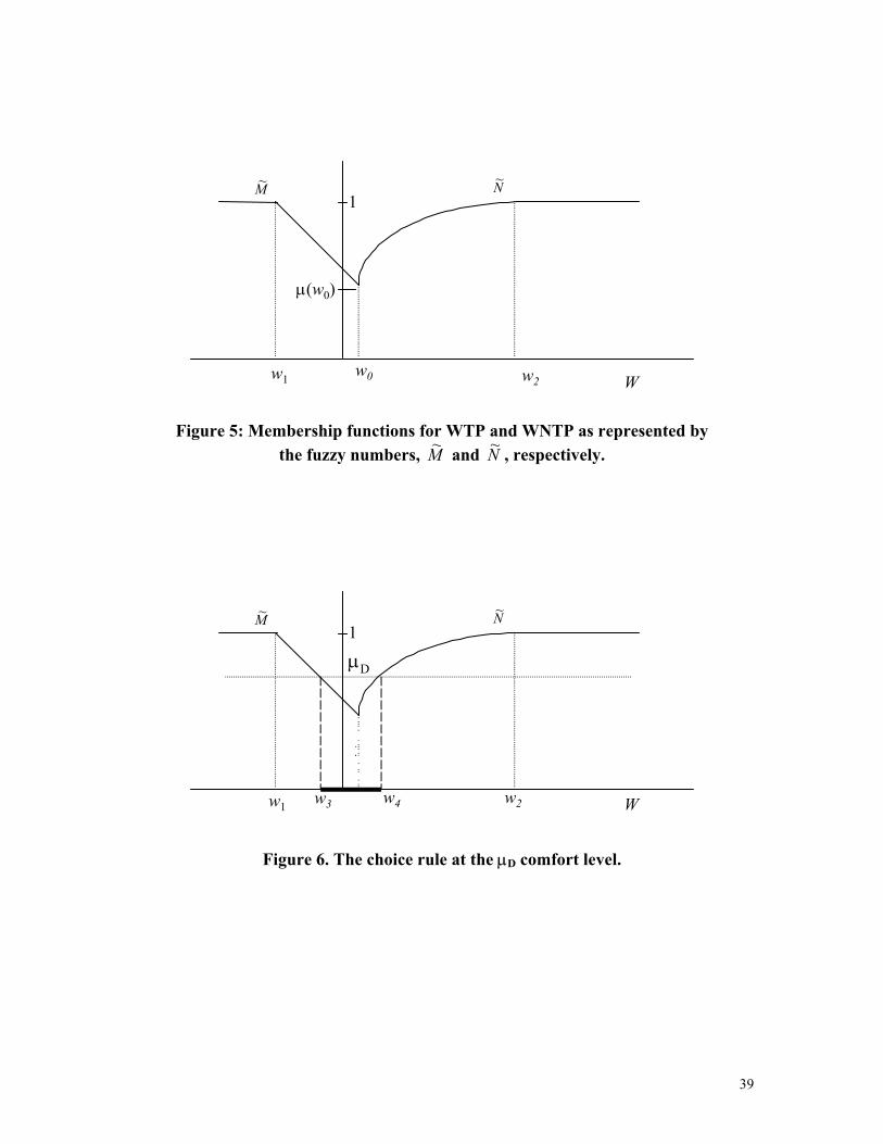
amounts) and then declines as the bid increases above w1 (Figure 5). A bid w0 is the

maximum value that a respondent would be WTP with a membership µ(w0). The same w0

is the minimum bid that a respondent would not be willing to pay at the comfort level

µ(w0). As the bid amount W increases, membership in WNTP increases (as bids increase

they become less acceptable for the respondent) and reaches 1 at w2 (Figure 5).

<INSERT FIGURE 5 ABOUT HERE>

Three components of the fuzzy numbers M~ and N~ correspond to different

aspects of a respondent’s preference uncertainty in the non-market valuation context.

First, the shape of the membership curves of M~ and N~ may depend on the respondent’s

attitude toward risk, thus explaining the asymmetrical feature of the two curves. Second,

µ(w0) reflects the strength of a respondent’s preference uncertainty regarding valuation of

the environmental amenity. A higher µ(w0) corresponds to weaker preference uncertainty.

Finally, the width of the interval [w1,w2] relates to the range of the bid values over which

a respondent’s preferences are uncertain.

For a bid w0, a respondent is indifferent (at the comfort level µ(w0)) between

accepting or rejecting the bid. When a respondent is certain of her preferences, then

µ(w0)=1 and w0=w1=w2. Thus, our approach to CV with vague preferences includes

preference certainty as a special case. Another extreme value, µ(w0)=0, corresponds to

4 Kriström (1997) and Loomis and Ekstrand (1998) also permit negative WTP values.

22

the situation of strongest preference uncertainty. In this case, there is no single bid in the

range of non-intersection that could be reported as a maximum value (with reasonable

comfort) that a respondent is WTP. This occurs in Figure 5 if M~ and N~ do not intersect,

in which case the degree of uncertainty is so great as to prevent a decision. This

represents the situation where respondents register protest votes by not answering the

valuation question.

Despite similarities to the classical method, our approach to CV with vague

preferences is peculiar. Classical CV requires one value (maximum WTP, denoted M) to

define a crisp choice function. The choice rule is far more complex when vague

preferences are considered and more information is required. This should not be treated

as a disadvantage of the proposed methodology, but rather as a way of incorporating real-

life complexity into traditional models of CV.

The objective now is to determine the membership function of WTP:

µWTP (W)= 1, W<w1 (17)

µWTP (W)= Cyes(W), w1 ≤W≤w0.

Here, Cyes(W) is monotonically decreasing for W∈[w1, w0]. Likewise, the degree of

membership in WNTP is

µWNTP(W) = Cno(W), w0 ≤W≤w2 (18)

µWNTP(W) = 1, W>w2,

where Cno(W) is a monotonically increasing function for W∈[w0,w2] (see Figure 5). Once

the membership functions for WTP and WNTP are determined, the point of their

intersection (w0,µ(w0)) will be used to formulate the operational choice rule:

23

Fuzzy choice rule.

(a) Accept the bid W≤w0 with comfort Cyes(W)=µ(W)≥µ(w0), where µ(W)=µWTP(W).

(b) Reject the bid W>w0 with comfort Cno(W)=µ(W)≥µ(w0), where µ(W)=µWNTP(W).

For low µ(w0) value, the fuzzy choice rule is of no practical value because of the low

comfort with respect to the chosen ‘yes’ or ‘no’ answer. To overcome this problem, one

may wish to consider only answers to the DC question at the (arbitrary) comfort level

µD>µ(w0). Denote by w3 and w4 the maximum WTP and minimum WNTP, respectively,

with the µD comfort level (Figure 6). In this case, a respondent would be indifferent at the

µD level between ‘yes’ and ‘no’ answers to a DC question for all bids W∈[w3, w4].

<INSERT FIGURE 6 ABOUT HERE>

5. Case Study: Valuing Forest Preservation in Sweden

In this section, fuzzy WTP and WNTP numbers are constructed using the results of a

contingent valuation survey of Swedish residents undertaken during the summer of 1992

(Li and Mattsson 1995). The survey asked respondents whether they would be willing to

pay a given amount “… to continue to visit, use, and experience the forest environment

as [they] usually do.” Bid amounts took one the following values: 50, 100, 200, 400, 700,

1000, 2000, 4000, 8000 and 16000 SEK. Since Li and Mattsson were interested in

preference uncertainty, they used a post-decisional confidence measure based on a

follow-up question that asked respondents how certain they were about their ‘yes/no’

answer. A graphical scale with 5% intervals was used. The researchers also collected data

24

on household income, the respondent’s age, gender, education level, and average annual

number of forest visits. The sample consisted of 800 individuals living in Vasterbotten

county in Sweden. Although 436 questionnaires were returned, only 389 survey

responses were usable and provided to us.

We first assume that an individual’s response to the question of how certain she is

about her answer to the dichotomous choice question is a measure of the uncertainty of

WTP and WNTP in the case of ‘yes’ and ‘no’ responses, respectively. If a respondent

answers ‘yes’ with a comfort Cyes(W) to the dichotomous choice question at the bid value

W, it is assumed she would then be willing to pay any lesser amount than W with a

comfort at least as high as Cyes(W). It is also assumed that a maximum WTP value greater

than W may exist, but with a comfort level not greater than Cyes(W). Similar logic holds

for ‘no’ answers and minimum WNTP.

Using the same criterion as Li and Mattsson to eliminate observations,5 the

sample data were divided into two groups according to the respondents’ answers to the

dichotomous choice contingent question. To estimate the membership function for WTP,

we regress comfort level for the ‘yes’ answer on the relative bid expressed as a

percentage of the respondent’s income. Similarly, we regress comfort level for the ‘no’

answer on the respondent’s relative bid to estimate the membership function for WNTP.

Functional forms for fitting the sample data must satisfy both conditions (17) and (18).

Membership functions for aggregated WTP and WNTP are estimated from

available data using a statistical approach for constructing membership functions (see

5The authors exclude observations with income levels below 11,000 SEK and above 300,000 SEK, and those with education levels below 1 year and above 25 years of education (to eliminate cases where education exceeds age) (C–Z. Li, pers. cor.).

25

Chameau and Santamarina 1987). Instead of individual WTP and WNTP, estimated

membership functions of aggregate WTP and WNTP are developed. For data (Wi,µi),

i=1,2, …, n, and choice of a suitable functional form, membership functions can be

estimated using the method of least-squares. Once the parameter values a, b, … are

determined, then

(19) µ(W) = max[0, min(1, f(W, a, b, …)] , ∀W.

Different classes of functional forms are used in the literature to construct membership

functions, with Turksen (1991) providing a review of different approaches. We selected

two nonlinear forms of membership function that can cover a broad range of applications

(Sakawa 1993). The functional form used for ‘yes’ responses is:

(20) 21)(tanh 1

~ ++= − cbWaMµ , a, b, c ∈ℜ and a>0 .

The minimum of the sum of squared deviations of the respondents’ post–decisional

comfort levels is reached for estimated parameter values, a=1.775, b= –0.026 and

c=0.187.

The functional form employed for ‘no’ responses is:

(21) 21)tanh(

21)(~ ++= edWxNµ , d, e∈ℜ and d>0.

The minimum of the sum of squared deviations of the respondents’ post-decisional

comfort levels is obtained for d = 0.044 and e = 0.466.

Our estimate of the intersection of the membership of maximum WTP and

minimum WNTP occurs at a comfort level of 74.9% and is associated with the relative

26

bid of 1.82% of income.6 As the average income in the given sample is 171190 SEK, the

intersection of the two membership functions is associated with 3116 SEK. This value

may be interpreted as the respondents’ WTP with a comfort of 74.9%, but it is also the

respondents’ WNTP with 74.9% comfort. It is thus the largest estimated value of the

amenity for which there is an aggregate indifference between WTP and WNTP. Other

measures of welfare may be reported if higher comfort levels than 0.749 are applied. In

that case, we can report the WTP at the comfort level c>0.749 (which will be below 3116

SEK) and the WNTP at the level c (which will be above 3116 SEK) (see Figure 6). The

range of values between WTP and WNTP could be interpreted as the aggregated

indifference at the comfort level c.

To analyze the sensitivity of the fuzzy estimates to the form of the membership

functions, linear and exponential specifications for WTP and WNTP are also considered.

Upon regressing the respondents’ post-decisional comfort levels for both ‘yes’ and ‘no’

responses on the relative bid, we obtain the following respective membership functions

for WTP and WNTP:

(22) Linear: xxM 655.4461.83)(~ −=µ and xxN 071.1883.72)(~ +=µ

(23) Exponential:

)552.1210.0exp(1

1)(~−+

=x

xMµ and)932.0088.0exp(1

1)(~−−+

=x

xNµ .

As indicated in Table 1, the results are not sensitive to functional form. The estimates of

WTP provided using our fuzzy approach are lower than those of Li and Mattsson (1995).

Our estimate of maximum WTP (at about 75% comfort) ranges from 3116 SEK to 3561

6This is found by solving: 1.77 tanh–1(–0.026W+0.187) = 0.5 tanh(0.044W+0.466).

27

SEK is less than half the magnitude of Li and Mattsson’s lowest estimates—7352 SEK or

8578 SEK depending on what assumptions are made.

Table 1: Intersection of WTP and WNTP Membership Functions: Comparison of Different Functional Specifications Hyperbolic tangent Linear Exponential Proportion of income 1.82% 1.85% 2.08% Income level 3116 SEK 3167 SEK 3561 SEK Comfort level 0.749 0.749 0.753

Several explanations for the difference between Li and Mattsson’s and our results

are possible. The one that accounts for the major difference is that Li and Mattsson use

mean WTP as a measure of welfare. If we assume complementarity of the ‘yes’ and ‘no’

answers (as Li and Mattsson do), i.e., Cyes(W)=1–Cno(W), then the membership functions

of WTP and WNTP would intersect at (w0, 0.5) and the value w0 would correspond to the

median WTP. In that sense, it would be more appropriate to compare our measure with

the median WTP.7 Further, we make different assumptions about the nature of preference

uncertainty (as discussed in the introduction).

Asymmetry of the membership functions for WTP and WNTP may be explained

by different attitudes towards acceptance and non-acceptance of a particular bid.

Complete certainty of a ‘no’ answer occurs only for very high bid values, but respondents

choose not to accept a wide range of bid values including low ones. Respondents indicate

their uncertainty about an exchange of money for an environmental amenity through

expressed comfort levels that are below 1. We found that respondents indicate preference

7 Estimates of median WTP are usually lower than mean WTP, but Li and Mattsson (1995) do not report median WTP for forest preservation and we can only guess at what these values might be.

28

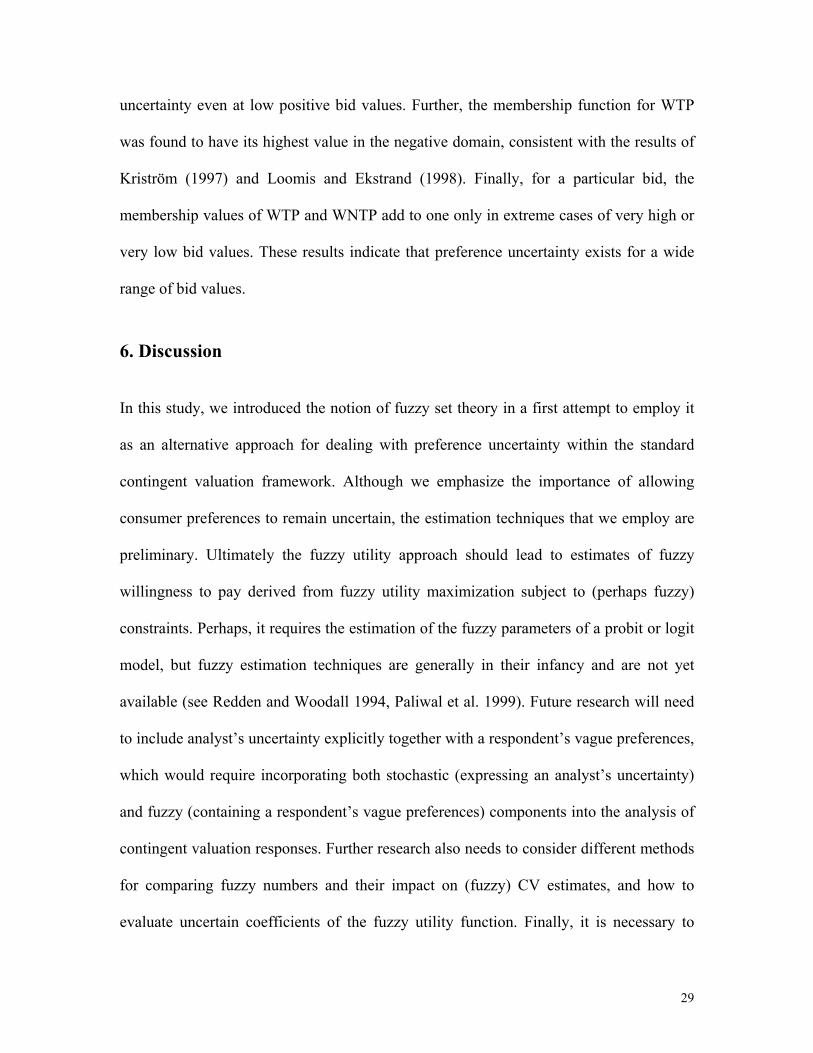
uncertainty even at low positive bid values. Further, the membership function for WTP

was found to have its highest value in the negative domain, consistent with the results of

Kriström (1997) and Loomis and Ekstrand (1998). Finally, for a particular bid, the

membership values of WTP and WNTP add to one only in extreme cases of very high or

very low bid values. These results indicate that preference uncertainty exists for a wide

range of bid values.

6. Discussion

In this study, we introduced the notion of fuzzy set theory in a first attempt to employ it

as an alternative approach for dealing with preference uncertainty within the standard

contingent valuation framework. Although we emphasize the importance of allowing

consumer preferences to remain uncertain, the estimation techniques that we employ are

preliminary. Ultimately the fuzzy utility approach should lead to estimates of fuzzy

willingness to pay derived from fuzzy utility maximization subject to (perhaps fuzzy)

constraints. Perhaps, it requires the estimation of the fuzzy parameters of a probit or logit

model, but fuzzy estimation techniques are generally in their infancy and are not yet

available (see Redden and Woodall 1994, Paliwal et al. 1999). Future research will need

to include analyst’s uncertainty explicitly together with a respondent’s vague preferences,

which would require incorporating both stochastic (expressing an analyst’s uncertainty)

and fuzzy (containing a respondent’s vague preferences) components into the analysis of

contingent valuation responses. Further research also needs to consider different methods

for comparing fuzzy numbers and their impact on (fuzzy) CV estimates, and how to

evaluate uncertain coefficients of the fuzzy utility function. Finally, it is necessary to

29

develop an appropriate survey instrument that allows respondents to express their

preference uncertainty qualitatively, rather than relying on data generated from CV

surveys that essentially require crisp responses. Indeed, it is likely necessary to develop

survey instruments that also treat fuzziness due to vagueness in classification (see Li

1989).

At this stage, it is not possible to say that the fuzzy approach is somehow ‘better’

than standard approaches for evaluating environmental amenities. The fuzzy approach to

contingent valuation interprets uncertainty in a fundamentally different way than the

standard random utility maximization model. Our results indicate persistence of

preference uncertainty over a wide range of bid values, thus suggesting that uncertainty

cannot be treated only as a random phenomenon to be minimized by providing

respondents with more information. In that case, the fuzzy approach needs to be seriously

considered as a method for addressing preference uncertainty in non-market valuation.

30

References

Banerjee, A., 1995. Fuzzy choice functions, revealed preference and rationality, Fuzzy

Sets and Systems 70: 31–43.

Barrett, C.R. and P.K. Pattanaik, 1989. Fuzzy Sets, Preference and Choice: Some

Conceptual Issues, Bulletin of Economic Research 41(4): 229–253.

Barrett, C.R., P.K. Pattanaik and M. Salles, 1990. On choosing rationally when

preferences are fuzzy, Fuzzy Sets and Systems 34: 197–212.

Basu, K., 1984. Fuzzy Revealed Preference Theory, Journal of Economic Theory 32:

212–27.

Bulte, E.H. and G.C. van Kooten, 1999. Marginal Valuation of Charismatic Species:

Implications for Conservation, Environmental and Resource Economics 14: 119-

130.

Chameau, J.L. and J.C. Santamarina, 1987. Membership Functions I, International

Journal of Approximate Reasoning 1(3): 287–301.

Chen, S.–J. and C.–L. Hwang, 1992. Fuzzy Multiple Attribute Decision Making: Methods

and Applications. New York: Springer–Verlag.

Cox, E., 1994. The Fuzzy Systems Handbook. Cambridge, MA: Academic Press.

Cutello, V. and J. Montero, 1997. Equivalence and compositions of fuzzy rationality

measures. Fuzzy Sets and Systems 85: 31–43.

Ells, A., E.H. Bulte, and G.C. van Kooten, 1997. Uncertainty and Forest Land Use

Allocation in British Columbia: Vague Preferences and Imprecise Coefficients,

Forest Science 43(4): 509–520.

31

Fedrizzi, M., 1987. Introduction to Fuzzy Sets and Possibility Theory. In Optimization

Models Using Fuzzy Sets and Possibility Theory edited by J. Kacprzyk and S.A.

Orlovski. Dordecht, The Netherlands: D. Reidel Publishing Co.

Gregory, R., S. Lichtenstein and P. Slovic, 1993. Valuing Environmental Resources: A

Constructive Approach, Journal of Risk and Uncertainty 7(October): 177–97.

Hanemann, W.M., 1984. Welfare Evaluations in Contingent Valuation Experiments with

Discrete Responses, American Journal of Agricultural Economics 66(August):

332–41.

Hanemann, W.M. and B. Kriström, 1995. Preference Uncertainty, Optimal Designs and

Spikes. Chapter 4 in Current Issues in Environmental Economics edited by P.–O.

Johansson, B. Ristrom and K.–G. Maler. Manchester UK: Manchester University

Press.

Hanley, N., J.F. Shogren and B. White, 1997. Environmental Economics in Theory and

Practice. Hampshire, NJ: MacMillan Press.

Hoehn, J. and A. Randall, 1987. A satisfactory benefit cost indicator from contingent

valuation, Journal of Environmental Economics and Management 14: 226-247.

Irwin, J.R., P. Slovic, S. Lichtenstein, and G.H. McClelland, 1993. Preference Reversals

and the Measurement of Environmental Values, Journal of Risk and Uncertainty

6(January): 5–18.

Kauffman, A. and M.M. Gupta, 1985. Introduction to Fuzzy Arithmetic. New York: Van

Nostrand Reinhold.

Klir, G. and T. Folger, 1988. Fuzzy Sets, Uncertainty, and Information. Englewood

Cliffs, New Jersey: Prentice Hall.

32

Klir, G.J. and B. Yuan, 1995. Fuzzy Sets and Fuzzy Logic. Englewood Cliffs, New

Jersey: Prentice Hall.

Knetsch, J.L., 2000. Environmental Valuations and Standard Theory: Behavioural

Findings, Context Dependence and Implications. Chapter 7 in The International

Yearbook of Environmental and Resource Economics 2000/2001 (pp.267-99)

edited by T. Tietenberg and H. Folmer. Cheltenham, UK: Edward Elgar.

Kosko, B., 1992. Neural Networks and Fuzzy Systems. Englewood Cliffs, NJ: Prentice

Hall.

Kriström, B., 1997. Spike Models in Contingent Valuation, American Journal of

Agricultural Economics 79(August): 1013–23.

Li, S., 1989. Measuring the Fuzzines of Human Thoughts: An Application of Fuzzy Sets

to Sociological Research, Journal of Mathematical Sociology 14(1): 67–84.

Li, C–Z. and L. Mattsson, 1995. Discrete Choice under Preference Uncertainty: an

Improved Structural Model for Contingent Valuation, Journal of Environmental

Economics and Management 28: 256–269.

Loomis, J. and E. Ekstrand, 1998. Alternative Approaches for Incorporating Respondent

Uncertainty when Estimating Willingness to Pay: The Case of the Mexican

Spotted Owl, Ecological Economics 27: 29–41.

McDaniels, T.L., 1996. The Structured Value Referendum: Eliciting Preferences for

Environmental Policy Alternatives, Journal of Policy Analysis and Management

15(2): 227–51.

33

Munda, G., P.Nijkamp and P. Rietveld, 1995. Qualitative Multicriteria Methods for

Fuzzy Evaluation Problems: An Illustration of Economic–Ecological Evaluation,

European Journal of Operational Research 82: 79–97.

Paliwal, R., G.A. Geevarghese, P.R. Babu and P. Khanna (1999) Valuation of landmass

degradation using fuzzy hedonic method: a case study of National Capital Region.

Environmental and Resource Economics 14: 519-543.

Ready, R.C., J.C. Whitehead and G.C. Blomquist, 1995. Contingent Valuation when

Respondents are Ambivalent, Journal of Environmental Economics and

Management 29: 181–196.

Redden, D. and W. Woodall, 1994. Properties of Certain Fuzzy Linear Regression

Methods, Fuzzy Sets and Systems 64: 361–375.

Saade, J.J. and H. Schwarzlander, 1992. Ordering Fuzzy Sets over the Real Line: An

Approach Based on Decision Making under Uncertainty, Fuzzy Sets and Systems

50: 237–246.

Sagoff, M., 1994. Should Preferences Count? Land Economics 70(May): 127–44.

Sakawa, M., 1993. Fuzzy Sets and Interactive Multiobjective Optimization. New York:

Plenum.

Treadwell, W.A., 1995. Fuzzy Set Theory Movement in the Social Sciences, Public

Administration Review 55(January/February): 91–96.

Turksen, I.B. 1991. Measurement of membership function. Fuzzy Sets and Systems 40(1):

5–38.

Zadeh, L.A., 1965. Fuzzy Sets, Information and Control 8: 338–53.

34

Yager, R.R., 1981. A procedure for ordering fuzzy subsets over the unit interval,

Information Science 24: 143–151.

35

f - d1 f f+d2

(x)F~µ

x

F~1.0

Figure 1: Non-symmetric triangular fuzzy number

α1

µ

S1 S4

S5

x

S3S2

F~ G~

f1 f2g1 g2

S5 S4S1

S2

α2

α1

µ

S1 S4

S5

x

S3S2

F~ G~

f1 f2g1 g2

S5 S4S1

S2

α2

µ

S1 S4

S5

x

S3S2

F~ G~

f1 f2g1 g2

S5 S4S1

S2

α2

Figure 2: Fuzzy numbers with nonempty intersection.

36

x

S3S2

µ(a)

S2

S5

x

S3

S1S4

µ

(c)

S5

x

S3S2

µ

(b)

F~ G~ F~ G~

G~F~

~ ~ ~ ~ ~ ~ ~ ~ ~ ~ ~ ~Figure 3: (a) s( F p G )=1, s( F f G )=0; (b) 0< s( F f G )<s( F p G )=1; ~ ~(c) 0<s( F~ p G )<1, 0<s( F~ f~ G~ )<1.

37

Environmental Amenity

γ

m-W

m

$

µ~ (A)

µ~ (B)

K

β

E0 E10

τ

π

Figure 4: Interpretation of Dichotomous Choice Answers with Fuzzy Utility

38

w0w1 W

N~M~1

w2

µ(w0)

Figure 5: Membership functions for WTP and WNTP as represented by the fuzzy numbers, M~ and N~ , respectively.

w1 w3 W

N~M~1

w2w4

µD

Figure 6. The choice rule at the µD comfort level.

39