Predictive Force Control of Robot Manipulators in … force control of robot manipulators in nonrigid environments 843 lis effects, as well as geometric and stiffness uncertainties

841

31

Predictive Force Control of Robot Manipulators

in Nonrigid Environments

L.F. Baptista, J.M.C. Sousa and J.M.G. Sa da Costa

1. Introduction

The application of robot manipulators in industry is in general related to tasks such as manipulation or painting that requires only position control of the arm. Nonetheless, there are other robotic tasks like pushing, polishing and grinding that require interaction between the manipulator and a contact sur-face or environment. This fact leads to the desire of controlling the interaction between the robot and the environment. Although a lot of different control schemes has been proposed in the literature, as surveyed by (Zeng & Hemami, 1997 ; De Schutter et al., 1997), the major force control approaches can be clas-sified as hybrid control (Raibert & Craig, 1981) or impedance control (Hogan, 1985). The hybrid control separates a robotic force task into two subspaces: a force controlled subspace and a position controlled subspace. Two independ-ent controllers are then designed for each subspace. In contrast, impedance control does not attempt to control force explicitly but rather to control the re-lationship between force and position of the end-effector in contact with the environment. Furthermore, when the environment is rigid with known charac-teristics it is possible to plan a virtual trajectory, such that a desired force pro-file is obtained (Singh & Popa, 1995). However, the same does not hold in the presence of nonrigid environments, which disables a reliable application of the classical impedance controller. This problem has motivated the development and design of more sophisticated force control methodologies which usually take into consideration the dynamics of the environment. In (Love & Book, 1995) it is shown that the performance of an impedance controlled manipula-tor increases when the desired impedance includes some modeling of the envi-ronment. Another possible solution to tackle this problem is to use a model-based control scheme like predictive control, which incorporates the manipula-tor and environment models in a force optimization-based strategy (Wada et al., 1993). Recently, a force control strategy for robotic manipulators in the presence of nonrigid environments combining impedance control and a model predictive control (MPC) algorithm in a force control scheme has been pro-posed (Baptista et al., 2000b). In this force control methodology, the predictive

842 Industrial Robotics: Theory, Modelling and Control

controller generate the position and velocity references in the constrained di-rection, to obtain a desired force profile acting on the environment. The main advantage of this control strategy is to provide an easy inclusion of the envi-ronment model in the controller design and thus to improve the global per-formance of the control system. Usually, impedance and environmental models are linear, mainly because the solution of an unconstrained optimization procedure can be analytically ob-tained with moderate computational burden. However, a nonrigid environ-ment has in general a nonlinear behavior, and a nonlinear model for the con-tact surface must be considered. Therefore, in this paper the linear spring/damper parallel combination, often used as a model of the environ-ment, is replaced by a nonlinear one, where the damping effect depends on the penetration depth (Marhefka & Orin, 1996). Unfortunately, when a nonlinear model of the environment is used, the resulting optimization problem to be solved in the MPC scheme is nonconvex. This problem can be solved using discrete search techniques, such as the branch-and-bound algorithm (Sousa et al., 1997). This discretization, however, introduces a tradeoff between the number of discrete actions and the performance. Moreover, the discrete ap-proximation can introduce oscillations around non-varying references, usually know as the chattering effect, and slow step responses depending on the se-lected set of discrete solutions. These effects are highly undesirable, especially in force control applications. A possible solution to this problem is a fuzzy scaling machine, which is proposed in this paper. Fuzzy logic has been used in several applications in robotics. In the specific field of robot force control, some relevant references, such as (Liu, 1995 ; Corbet et al., 1996 ; Lin & Huang, 1997), can be mentioned. However, these papers use fuzzy logic in the classic low level form, while in this paper fuzzy logic is applied in a higher level. Here, the fuzzy scaling machine alleviates the effects due to the discretization of the nonconvex optimization problem to be solved in the model predictive algo-rithm, which derives the virtual reference for the impedance controller consid-ering a nonlinear environment. The fuzzy scaling machine proposed in this paper uses an adaptive set of discrete alternatives, based on the fulfillment of fuzzy criteria applied to force control. This approach has been used in predic-tive control (Sousa & Setnes, 1999), and is generalized here for model predic-tive algorithms. The adaptation is performed by a scaling factor multiplied by a set of alternatives. By using this approach, the number of alternatives is kept low, while performance is increased. Hence, the problems introduced by the discretization of the control actions are highly diminished. For the purpose of performance analysis, the proposed predictive force control strategy with fuzzy scaling is compared with the impedance controller with force tracking by simulation with a two-degree-of-freedom (2-DOF) manipula-tor, considering a nonlinear model of the environment. The robustness of the predictive control scheme is tested considering unmodeled friction and Corio-

Predictive force control of robot manipulators in nonrigid environments 843

lis effects, as well as geometric and stiffness uncertainties on the contact sur-face. The implementation and validation of advanced control algorithms, like the one presented above, require a flexible structure in terms of hardware and software. However, one of the major difficulties in testing advanced force/position control algorithms relies in the lack of available commercial open robot controllers. In fact, industrial robots are equipped with digital con-trollers having fixed control laws, generally of PID type with no possibility of modifying the control algorithms to improve their performance. Generally, ro-bot controllers are programmed with specific languages with fixed pro-grammed commands having internally defined path planners, trajectory inter-polators and filters, among other functions. Moreover, in general those controllers only deal with position and velocity control, which is insufficient when it is necessary to obtain an accurate force/position tracking performance (Baptista et al., 2001b). Considering these difficulties, in the last years several open control architectures for robotic applications have been proposed. Gener-ally, these solutions rely on digital signal processor techniques (Mandal & Payandeh, 1995 ; Jaritz & Spong, 1996) or in expensive VME hardware running under the VxWorks operating system (Kieffer & Yu, 1999). This fact has moti-vated the development of an open PC-based software kernel for management, supervision and control. The real-time software tool for the experimentation of the algorithms proposed in this paper was developed considering require-ments such as low cost, high flexibility and possibility of incorporating new hardware devices and software tools (Baptista, 2000a). This article is organized as follows. Section 2 summarizes the manipulator and the environment dynamic models. The impedance controller with force track-ing is presented in section 3. Section 4 presents the model predictive algorithm with fuzzy scaling applied to force control. The simulation results for a 2-DOF robot manipulator are discussed in section 5. The experimental setup and the force control algorithms implemented in real-time are presented in section 6. The experimental results with a 2-DOF planar robot manipulator are presented in section 7. Finally, some conclusions are drawn in section 8.

2. Manipulator and environment modeling

Consider an n-link rigid-link manipulator constrained by contact with the en-vironment, as shown in fig.1. The complete dynamic model is described by (Si-ciliano & Villani, 2000)

( ) ( , ) ( ) ( ) eM q q C q q q g q d q τ τ+ + + = −&& & & & (1)


where 1, , ×∈& && nq q q R correspond to the joint, position, velocity and acceleration vectors, respectively, ( ) ×∈ n nM q R is the symmetric positive definite inertia ma-trix, ( , ) ×∈& n nC q q R is the centripetal and Coriolis matrix, 1( ) ×∈ ng q R contains the gravitational terms and 1( ) ×∈& nd q q R accounts for the frictional terms. The vec-tor 1×∈ nRτ is the joint input torque vector and 1×∈ n

e Rτ denote the generalized vector of joint torques exerted by the environment on the end-effector. From (1) it is possible to derive the robot dynamic model in the Cartesian space:

( ) ( , ) ( ) ( )x x x x eM x x C x x x g x d x f f+ + + = −&& & & & (2) where x is the n-dimensional vector of the position and orientation of the ma-nipulator's end-effector, 1( )− ×= ∈T nf J q Rτ is the robot’s driving force,

1×∈ nef R is the contact force vector and J represents the Jacobian matrix.

The interaction force vector [ ]Te n tf f f= is composed by the normal contact force fn and the tangential contact forces ft caused by friction contact between the end-effector and the surface. An accurate modeling of the contact between the manipulator and the environment is usually difficult to obtain due to the complexity of the robot's end-effector interaction with the environment. In this paper, the normal contact force fn is modeled as a nonlinear spring-damper mechanical system according (Marhefka & Orin, 1996):

( )n ef ke x x xδ ρ δ= + & (3) where the terms ke and ρe are the environment stiffness and damping coeffi-cients, respectively, ex x xδ = − is the penetration depth, where xe stands for the distance between the surface and the base Cartesian frame. Notice that the damping effect depends non-linearly on the penetration depth δx. The tangen-tial contact force vector ft due to surface friction is assumed to be given as proposed by (Yao & Tomizuka, 1995):

sgn( )t n pf f xμ= & (4) where px& is the unconstrained or sliding velocity and μ is the dry friction coef-ficient between the end-effector and the contact surface.


Figure 1. Robot manipulator applying a desired force on the environment. (Reprinted from Baptista, L.; Sousa, J. & Sá da Costa, J. (2001a) with kind permission of Springer Science and Business Media).

3. Impedance control

The impedance controller proposed by (Hogan, 1985) aims at controlling the dynamic relation between the manipulator and the environment. The force ex-erted by the manipulator on the environment depends on the end-effector po-sition and the correspondent impedance. The impedance of the robot is di-vided in the following terms: one that is physically intrinsic to the manipulator and the other that is given to the robot by the controller. The impedance con-trol goal is to oblige the manipulator to follow the reference or target imped-ance. As shown by (Volpe & Khosla, 1995) a good impedance relation is achieved with a linear model of second order. The complete form of a second order type impedance control model, which is valid for free or constrained motion, is given by:

( ) ( )d d d d d eM x B x x K x x f− − − − = −&& & & (5) where ,d dx x& are the desired velocity and position defined in the Cartesian space, respectively, and ,x x& are the end-effector velocity and position in Car-tesian space, respectively. The matrices , ,d d dM B K are the desired inertia, damping and stiffness for the manipulator. The reference or target end-effector acceleration u x≡ && is then given by:

1( )d d d eu M B e K e f−= + −& (6)


where , d de x x e x x= − = −& & & are the velocity and position errors, respectively. Thus, u can be used as the command signal to an inner position control loop in order to drive the robot accordingly to the desired trajectory.

3.1 Virtual trajectory for force tracking

The major drawback of the impedance control scheme presented above is re-lated to its poor force tracking capability, especially in the presence of nonrigid environments (Baptista et al., 2000b). However, from the conventional imped-ance control scheme it is possible to obtain a force control scheme in a steady-state contact condition with the surface. Considering the impedance control scheme (6) in the constrained direction, the following holds:

1( ( ) ( ) )f d d v d v nu m b x x k x x f−= − + − −& & (7) where , and v v fx x u& are the virtual position, velocity and target acceleration, re-spectively, while , ,d d dm b k are appropriate elements of , ,d d dM B K matrices de-fined in (5) in the constrained direction. The contact force fn during steady-state contact with the surface is given by:

( )n d vf k x x= − (8) Considering for simplicity the environment modeled by a linear spring with stiffness ke the contact force is given by: n ef k xδ= (9)

This leads to the following steady-state position and contact force (Singh & Popa, 1995):

d v e ess

d e

k x k xxk k

+=+

(10)

( )

ss

d en v e

d e

k kf x xk k

= −+

(11)

It is possible to apply a desired force fd on the system while simultaneously achieving the desired impedance by estimating the desired virtual position xv as:


e dv e d

e d

k kx x fk k

⎛ ⎞+= + ⎜ ⎟⎝ ⎠

(12)

Moreover, when the environment stiffness is unknown, it is also possible to obtain the virtual position from fd, fn and δx (Jung & Hsia, 1995). In this case, by substitution of ke in (12) the following virtual position xv is obtained:

if 0

if 0

de n

dv

d ne d n

d n

fx fk

xk x fx f fk fδ

⎧ + =⎪⎪= ⎨ ⎛ ⎞+⎪ + ≠⎜ ⎟⎪ ⎝ ⎠⎩

(13)

which is valid for contact and non-contact condition. This approach enables the classical impedance controller, given by (6), with force tracking capability without explicit knowledge of the environment stiffness. Notice that vx& is usu-ally assumed to be zero due to the noise always present in the force sensor measurements.

3.2 Impedance control with force tracking

The impedance control with force tracking (ICFT) block diagram is presented in fig.2.

ef

d dx ,x&

qq & ,

vx

uτ

xx & ,

Inverse dynamics controller

Impedance controller

Force sensor/ environment

Robot

Reference trajectory algorithm

df Forward kinematics

Figure 2. Impedance control with force tracking (ICFT) block diagram. In this scheme, the virtual position xv given by (13), is computed in the Refer-ence trajectory algorithm block, while the target acceleration vector


T

f pu u u⎡ ⎤= ⎣ ⎦ with up is obtained from (6) and uf from (7), is computed in the Impedance controller block. Moreover, the unconstrained target acceleration vec-tor up is further compensated by a proportional-derivative (PD) controller, which is given by: pc p P Du u K e K e= + + & (14)

where KP and KD are proportional and derivative gain matrices, respectively. The target acceleration vector

T

c f pcu u u⎡ ⎤= ⎣ ⎦ is then used as the driving signal to the inverse dynamics controller, in order to track the desired force profile. Since robot controllers are usually implemented in the joint space, it is useful to obtain the correspondent target joint acceleration uq for the inverse dynam-ics controller. Then, using the appropriate kinematics transformations, uq is given by:

( )1 ( )q cu J u J q q−= − & & (15) Then, applying an inverse dynamics controller in the inner control loop, the joint torques are given by:

ˆ ˆ( ) ( ) ( )Tq eM q u g q J q fτ = + + (16) where ˆ ˆ( ), ( )M q g q are estimates of ( ), ( )M q g q in the robot dynamic model (1). Notice that Coroilis and friction effects are neglected. The impedance control-ler with force tracking (ICFT) presented above is a good control approach for rigid environments since the end-effector velocity in the constrained direction is close to zero, which leads to a virtual position with an acceptable precision. However, for nonrigid environments the constrained velocity can hardly be zero, which limits the accuracy of the control system to track the desired force profile (Baptista et al, 2001a). To overcome the drawbacks of the scheme pre-sented above, this paper proposes an alternative force control methodology based on a model predictive algorithm (MPA) which is presented in the next section.


4. Model predictive algorithms applied to force control

Predictive algorithms consist of a broad range of methods, which are used to predict a desired variable in an optimal way. The most common predictive al-gorithms are model predictive controllers (Maciejowski, 2002), which have one common feature; the controller is based on the prediction of the future system behavior by using a process model. In a more general way, predictive algo-rithms are based on the following basic concepts:

1. Use of a (nonlinear) model to predict the process outputs at future time periods over a prediction horizon;

2. Computation of a sequence of future inputs using the model of the sys-tem by minimizing a certain objective function;

3. Receding horizon principle; at each sampling period the optimization process is repeated with new measurements, and only the first input ob-tained is applied to the system.

In this paper, an MPA is used to predict the target position xv to the impedance control law in (7), such that a desired force profile is obtained. In general, a predictive algorithm minimizes a cost function over a specified prediction ho-rizon Hp. In order to reduce model-plant mismatch and disturbances in an ef-fective way, the predictive algorithm is combined with an internal model con-trol (IMC) structure (Economou et al., 1986) which increases the force tracking performance. A filter is included in the feedback loop of the predictive struc-ture to reduce the noise present in the force sensor data. This filter stabilizes the loop by decreasing the gain, increasing the robustness of the force control loop. The sequence of future target positions ( )..... ( 1)v v px k x k H+ − over a speci-fied prediction horizon, produced by the MPA, results in a new target accel-eration by the impedance control law (6), which determines the force to apply on the surface. Predictive algorithms need a prediction model to compute the optimal input. In this paper, the model must predict the contact force fm based on the measured position x and velocity x& . This model must consider the dy-namics of the environment given by (3). In order to minimize the number of calculations during the nonlinear optimization procedure, only the virtual tra-jectory is computed in an optimal way, and thus vx& is assumed to be zero. Therefore, the nonlinear prediction model in the constrained direction is given by:

( )d f d d v mm u b x k x x f+ − − = −& (17) Note that a discrete version of this model is required, predicting the future val-ues fm(k+i) based on the measured position x(k) and the measured velocity


( )x k& at time instant k. The predictive scheme is combined with an internal model control scheme, and the model-plant mismatch is given by

( ) ( ) ( )m n me k f k f k= − (18) The desired force profile fd is compensated by the filtered modeling error emf, as shown in fig.4, resulting in the modified force reference fdc defined as:

( ) ( ) ( )dc d mff k f k e k= − (19) The cost function considered for the force control scheme is then given by:

( )2

1

( ) ( ) ( )pH

v dc mi

J x f k i f k i=

= + − +∑ (20)

The process inputs and outputs, as well as state variables, can be subjected to constraints, which must be incorporated in the optimization problem.

k

fdHc

Hp

fm

xv

fm

k-1 k+1 ... k+Hc... k+Hp

^

Figure 3. Basic principle of MPA applied to robot force control. The performance of the MPA depends largely on the accuracy of the process model. The model must be able to accurately predict the future process out-


puts, and at the same time be computationally attractive to meet real-time de-mands. When both nonlinear models and constraints are present, the optimi-zation problem is nonconvex. Efficient optimization methods for nonconvex optimization problems can be used when the solution space is discretized, and techniques such as Branch-and-Bound - B&B (Sousa et al., 1997) can be ap-plied. The B&B method can be used in a recursive way, demanding less com-putation effort than other methods, and is used in this paper to solve the non-convex optimization problem. Figure 3 presents the basic principle of a predictive strategy applied to robot force control.

4.1 Branch-and Bound Optimization

Branch-and-Bound algorithms solve optimization problems by partitioning the solution space. In this paper, B&B is used for the optimization problem that must be solved at each time instant k in the model predictive algorithm. A B&B algorithm can be characterized by two rules: Branching rule - defines how to divide a problem into sub-problems; and Bounding rule - establishes lower and upper bounds in the optimal solution of a sub-problem, allowing for the elimi-nation of sub-problems that do not contain an optimal solution. The model predicts the future outputs of the system, which are the forces

( 1),...., ( )m m pf k f k H+ + and can be given by (3) when the stiffness coefficient is considered to be constant. Let M be the possible discrete inputs of the system, which are denoted as w j. Thus, at each step the desired positions

( 1)vx k i+ − ∈Ω , are given by { 1, 2,..., }j j MωΩ = = . In the considered predictive scheme, the problem to be solved is represented by the objective function (20) minimizing the predicted force error. This opti-mization problem is successively decomposed by the branching rule into smaller sub-problems. At time instant k+i the cumulative cost of a certain path followed so far, and leading to the output fm(k+i) is given by

( )2( )

1

( ) ( )i

idc m

l

J f k l f k l=

= + − +∑ (21)

where i = 1,…,Hp, denotes the level corresponding to the time step k+i. A par-ticular branch j at level i is created when the cumulative cost ( ) ( )iJ u plus a lower bound on the cost from the level i to the terminal level Hp for the branch j, denoted

jLJ , is lower than an upper bound of the total cost, denoted JU :

( )

j

iL UJ J J+ < (22)


Let the total number of branches verifying this rule at level i be given by N. In order to increase the efficiency of the B&B method, it is required that this num-ber should be as low as possible, i.e. N M . The major advantages of the B&B algorithm applied to MPA over other non-convex optimization methods are the following: the global discrete minimum containing the optimal solution is always found, guaranteeing good perform-ance; and the B&B method implicitly deals with constraints. In fact, the pres-ence of constraints improve the efficiency of bounding, restricting the search space by eliminating non-feasible sub-problems. The most serious drawbacks of B&B are the exponential increase of the compu-tational time with the prediction horizon and the number of alternatives, and the discretization of the possible inputs, which are the position references xv in this paper. A solution to these problems is proposed in the next section.

4.2 Fuzzy scaling machine

Fuzzy predictive filters, as proposed in (Sousa & Setnes, 1999), select discrete control actions by using an adaptive set of control alternatives multiplied by a gain factor. This approach diminishes the problems introduced by the discreti-zation of control actions in MPA. The predictive rules consider an error in or-der to infer a scaling factor, or gain, ( ) [0,1]kγ ∈ for the discrete incremental in-puts. For the robotic application considered in this paper this error is given by em, as defined in (18). The gain ( )kγ goes to the zero value when the system tends to a steady-state situation, i.e., the force error and the change in this error are both small. On the other hand, the gain increases when the force error or the change in this error is high. When the gain ( )kγ is small, the possible inputs are made close to each other, diminishing to a great extent, or even nullifying, oscillations of the output. When the system needs to change rapidly the gain is increased and the interval of variation of the inputs is much larger, allowing for a fast response of the system. The fuzzy scaling machine reduces thus the main problem introduced by the discretization of the inputs, i.e. a possible limit cycle due to the discrete inputs, maintaining also the number of necessary input alternatives low, which increases significantly the speed of the optimiza-tion algorithm. The design of the fuzzy scaling machine consists of three parts: the choice of the discrete inputs, the construction of the fuzzy rules for the gain filter, and the application of the B&B optimization. The first two parts are ex-plained in the following. Let the virtual position ( 1)vx k X− ∈ , which was described in (17), represent the input reference at time instant 1k − , where [ , ]X X X− += is the domain of this reference position. Upper and lower bounds must be defined for the pos-sible changes in this reference signal at time k, which are respectively kx

+ and


kx− : ( 1)k vx X x k+ += − − , ( 1)k vx X x k− −= − − .

These values are then defined as the maximum changes allowed for the virtual reference when it is increased or decreased, respectively. The adaptive set of incremental input alternatives can now be defined as

{ }* 0, , ^ 1, ,k l k l kx x l Nλ λ+ −Ω = = K (23) The distribution lλ must be chosen taking into account that 0 1lλ≤ ≤ . In this way, the choice of lλ sets the maximum change allowed at each time instant by scaling the maximum variations kx

+ and kx− . The parameter l is important to

define the number of possible inputs. From (23) it follows that the cardinality of kΩ , i.e., the number of discrete alternatives, is given by 2 1M l= + . The fuzzy scaling machine applies a scaling factor, ( ) [0,1]kγ ∈ to the adaptive set of inputs *

kΩ in order to obtain the scaled inputs kΩ of the optimization routine, the B&B in this case:

*( )k kkγΩ = ⋅Ω (24) The scaling factor ( )kγ must be chosen based on the predicted error between the reference and the system's output, which is defined as

( ) ( ) ( ),p dc p n pe k H f k H f k H+ = + − + (25) where ( )dc pf k H+ is the reference to be followed at time pH , as in (19). Added to the error, the change in the error gives usually important indications on the evolution of the system behavior. This information can also be considered in the derivation of ( )kγ . The change in error is given by

( ) ( ) ( 1).e k e k e kΔ = − − (26) The fuzzy rules to be constructed have as antecedents the predicted error and the change in the error, and as consequent a value for the scaling factor. Simple heuristic rules can be constructed noticing the following. The system is close to a steady-state situation when the error and the change in the error are both small. In this situation, the discrete virtual references must be scaled down, al-lowing smaller changes in the reference vx , which yield smaller variations in the impedance controller, and ( )kγ should tend to zero. On the other hand, when the predicted error or the change in error are high, larger discrete refer-


ences must be considered, and ( )kγ should tend to its maximum value, i.e. 1. The trapezoidal and triangular membership functions ( ( ))e pe k Hμ + and

( ( ))e e kμΔ Δ define the two following fuzzy criteria: “small predicted error” and “small change in error”, respectively. The two criteria are aggregated using a fuzzy intersection; the minimum operator (Klir, 1995). In this way, the mem-bership degree of these criteria using the min operator is given by:

( ( ), ( )) min( , ),p e ee k H e kγμ μ μΔ+ Δ = (27) The scaling factor ( )kγ must be the fuzzy complement of a certain member-ship degree γμ :

( ) 1 .k γ γγ μ μ= = − (28) Summarizing, the set of inputs *

kΩ at time instant k, which are virtual refer-ences in this paper, is defined in (23). These inputs are within the available in-put space at time k. Further, the inputs are scaled by the factor ( ) [0,1]kγ ∈ to create a set of adaptive alternatives kΩ , which are passed on to the optimiza-tion routine. At a certain time k, the value of ( )kγ is determined by simple fuzzy criteria, regarding the predicted error of the system. Note that the pro-posed fuzzy scaling machine has only the following design parameters: lλ , and the membership functions eμ and eμΔ . Moreover, the tuning of these pa-rameters is not a hard task, allowing the use of some heuristics to derive them. Possible constraints on the input signal, which is the virtual trajectory in this paper, are implemented by selecting properly the parameters lλ .

Fuzzyscaling

machine

fd xv

-

Filter

Modelfm

em

-

+

+ fd c

emf

Internalcontrollerand robot

Internalcontrollerand robot

Environment

fn

x, x.

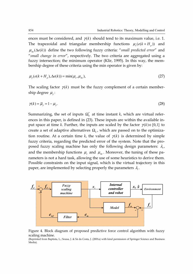
Figure 4. Block diagram of proposed predictive force control algorithm with fuzzy scaling machine. (Reprinted from Baptista, L.; Sousa, J. & Sá da Costa, J. (2001a) with kind permission of Springer Science and Business Media).


Figure 4 depicts the proposed predictive force control algorithm with fuzzy scaling. The block Fuzzy scaling machine contains the model predictive algo-rithm, the B&B optimization and the fuzzy scaling strategy. The block Internal controller and robot implement the impedance and the inverse dynamics control algorithms. The robot dynamic model equations are also computed in this block. The block Environment contains the nonlinear model of the environ-ment. In order to cope with disturbances and model-plant mismatches, an in-ternal model controller is included in the control scheme. The block Filter be-longs to the IMC structure (Baptista et al., 2001a).

5. Simulation results

The force control scheme introduced in this paper is applied to a robot through computer simulation for an end-effector force/position task in the presence of robot model uncertainties and inaccuracy in the environment location and the correspondent stiffness characteristics. The robot model represents the links 2 and 3 of the PUMA 560 robot. In all the simulations, a constant time step of 1 ms is used. The overall force control scheme including the dynamic model of the PUMA robot is simulated in the Matlab/Simulink environment. A nonri-gid friction contact surface is placed in the vertical plane of the robot work-space where it is assumed that the end-effector always maintain contact with the surface during the complete task execution. In order to analyze the force control scheme robustness to environment model-ing uncertainties, a non rigid time-varying stiffness profile ke(t) is considered, given by:

( 0.25( 2))

1000 sin( / 2) 0 2( )

1000 2 3e t

t tk t

e tπ

− −

+ < <⎧= ⎨ ≤ <⎩

(29)

The damping coefficient and the coefficient of dry friction are settled to ρe=45 Ns/m2 and μ=0.2, respectively. Notice that the stiffness coefficient is consid-ered to be constant (ke=1000 N/m) in the environment model used for predict the contact force fm. The matrices in the impedance model (6) are defined as Md

= diag[2.5 2.5] and Kd = diag[250 2500] to obtain an accurate force tracking in the x-axis direction and an accurate position tracking performance in the y-axis direction. The matrix Bd is computed to obtain a critically damped system behavior. The control scheme was tested considering a smooth step force profile of 10 N and a desired position trajectory from p1 = [0.5 -0.2] m to p2 = [0.5 0.6] m. Uncertainties in the location of the contact surface given by the final real posi-tion of p2r=[0.512 0.6] m are considered in the simulations, as shown in fig.5.


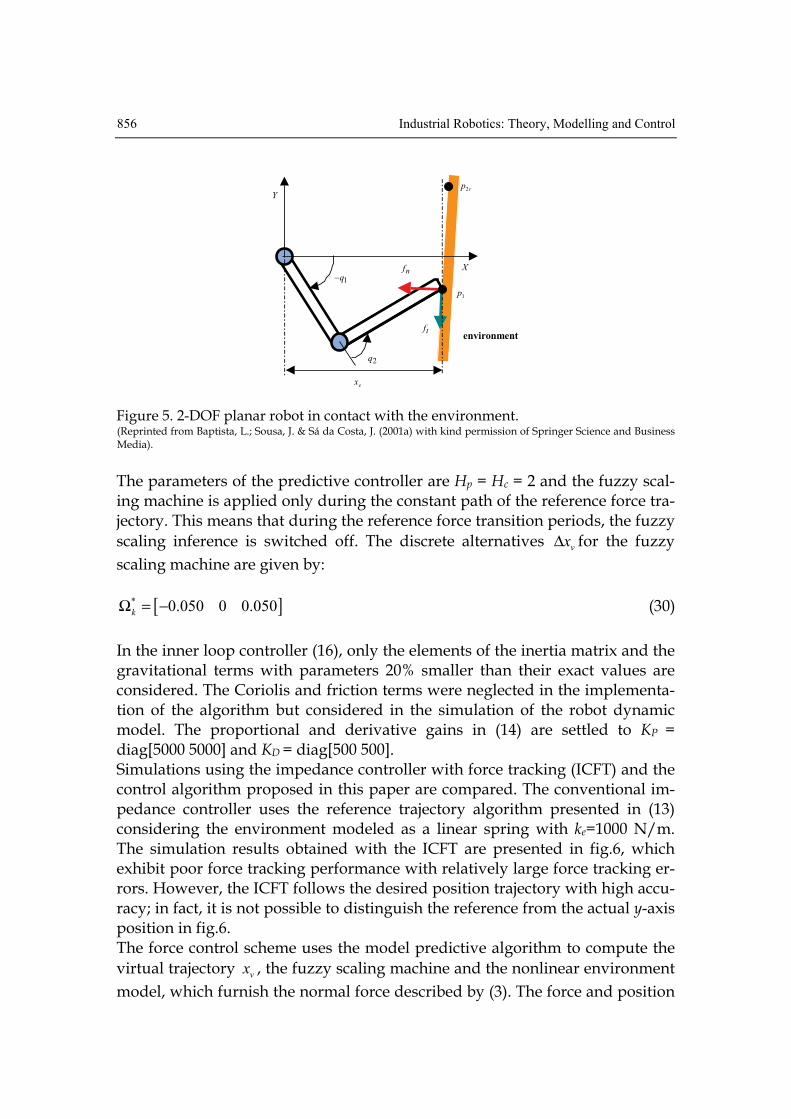
Figure 5. 2-DOF planar robot in contact with the environment. (Reprinted from Baptista, L.; Sousa, J. & Sá da Costa, J. (2001a) with kind permission of Springer Science and Business Media).

The parameters of the predictive controller are Hp = Hc = 2 and the fuzzy scal-ing machine is applied only during the constant path of the reference force tra-jectory. This means that during the reference force transition periods, the fuzzy scaling inference is switched off. The discrete alternatives vxΔ for the fuzzy scaling machine are given by:

[ ]* 0.050 0 0.050kΩ = − (30) In the inner loop controller (16), only the elements of the inertia matrix and the gravitational terms with parameters 20% smaller than their exact values are considered. The Coriolis and friction terms were neglected in the implementa-tion of the algorithm but considered in the simulation of the robot dynamic model. The proportional and derivative gains in (14) are settled to KP = diag[5000 5000] and KD = diag[500 500]. Simulations using the impedance controller with force tracking (ICFT) and the control algorithm proposed in this paper are compared. The conventional im-pedance controller uses the reference trajectory algorithm presented in (13) considering the environment modeled as a linear spring with ke=1000 N/m. The simulation results obtained with the ICFT are presented in fig.6, which exhibit poor force tracking performance with relatively large force tracking er-rors. However, the ICFT follows the desired position trajectory with high accu-racy; in fact, it is not possible to distinguish the reference from the actual y-axis position in fig.6. The force control scheme uses the model predictive algorithm to compute the virtual trajectory vx , the fuzzy scaling machine and the nonlinear environment model, which furnish the normal force described by (3). The force and position


results from the application of this controller are presented in fig.7. Comparing this figure with fig.6, it becomes clear that the proposed force controller pre-sents a remarkable performance improvement in terms of force tracking capa-bility. In fact, it is not possible to distinguish the reference force from the actual contact force. In terms of position control, similar performance is achieved. The results for both controllers can be compared in Table 1, where the error norm . for position and force errors, as well as the absolute maximum values for these errors are presented. The table shows that the force control perform-ance is clearly superior for the MPA with fuzzy scaling machine.

Force control algorithms pe

[m]

Max(ep)

[mm] fe

[N]

Max(ef)

[N] Impedance control with force track-ing

0.041 0.836 60.426 4.420

MPA with fuzzy scaling machine 0.041 0.801 0.8021 0.064

Table 1. Euclidian norm of position, force errors and absolute maximum errors.

0 0.5 1 1.5 2 2.5 30

2

4

6

8

10

12

f d ;

f n ;

f t [N

]

0 0.5 1 1.5 2 2.5 3−0.4

−0.2

0

0.2

0.4

0.6

time [s]

y d ;

y [m

]

Figure 6. Impedance control with force tracking: desired force (dashdot), normal force (solid) and friction force (dashed) – top view; desired y-axis trajectory (dashdot) and actual position trajectory (solid) – bottom view. (Reprinted from Baptista, L.; Sousa, J. & Sá da Costa, J. (2001a) with kind permission of Springer Science and Business Media).


0 0.5 1 1.5 2 2.5 30

2

4

6

8

10

12

f d ;

f n ;

f t [N

]

0 0.5 1 1.5 2 2.5 3−0.4

−0.2

0

0.2

0.4

0.6

time [s]

y d ;

y [m

]

Figure 7. MPA with fuzzy scaling: desired force (dashdot), normal force (solid) and friction force (dashed) – top view; desired y-axis trajectory (dashdot) and actual posi-tion trajectory (solid) – bottom view. (Reprinted from Baptista, L.; Sousa, J. & Sá da Costa, J. (2001a) with kind permission of Springer Science and Business Media).

0 0.5 1 1.5 2 2.5 3−0.08

−0.06

−0.04

−0.02

0

0.02

e f [

N]

0 0.5 1 1.5 2 2.5 30

0.2

0.4

0.6

0.8

1

time [s]

γ(k

)

Figure 8. MPA with fuzzy scaling: contact force errors (top view) and fuzzy scaling factor γ(k) (bottom view). (Reprinted from Baptista, L.; Sousa, J. & Sá da Costa, J. (2001a) with kind permission of Springer Science and Business Media).


0 0.5 1 1.5 2 2.5 340

50

60

70

80

90

τ1

[Nm

]

0 0.5 1 1.5 2 2.5 340

50

60

70

80

90

time [s]

τ1

[Nm

]

Figure 9. MPA with fuzzy scaling: joint torque τ1 without (top view) and with fuzzy scaling machine (bottom view). (Reprinted from Baptista, L.; Sousa, J. & Sá da Costa, J. (2001a) with kind permission of Springer Science and Business Media). In order to study in more detail the proposed force approach, fig. 8 presents the contact force error and the fuzzy scaling factor γ(k) for the same trajectory. The factor γ(k) exhibits a fast convergence to values around zero during the constant reference force path, which reduces the chattering present on the tar-get trajectory and in the joint torques. The joint torque τ1 using the predictive approach with and without the fuzzy scaling machine is shown in fig. 9. The strategy without fuzzy scaling produce undesirable oscillations on the virtual trajectory xv, which has the same effect on the joint torques τ. This effect is significantly reduced by the fuzzy scaling machine, as shown in fig.9 for the joint torque τ1.

6. Experimental setup

In order to validate the proposed force control scheme presented in previous sections, real-time experiments were carried out with a 2-DOF planar manipu-lator and a nonrigid mechanical environment built at the Robotics Laboratory of Technical University of Lisbon/Instituto Superior Técnico (IST). A low cost open PC-based control architecture using a commercial servo-axis interface board was developed to control the robotic setup in an effective and reliable way.


.m I2 2,

l1

.

l2

m I1 1,

lc1

lc2

q1

q2

X

shaft

Force sensor

Y

fz

fx

springspring

ye

fn

shaft

Rigid plate

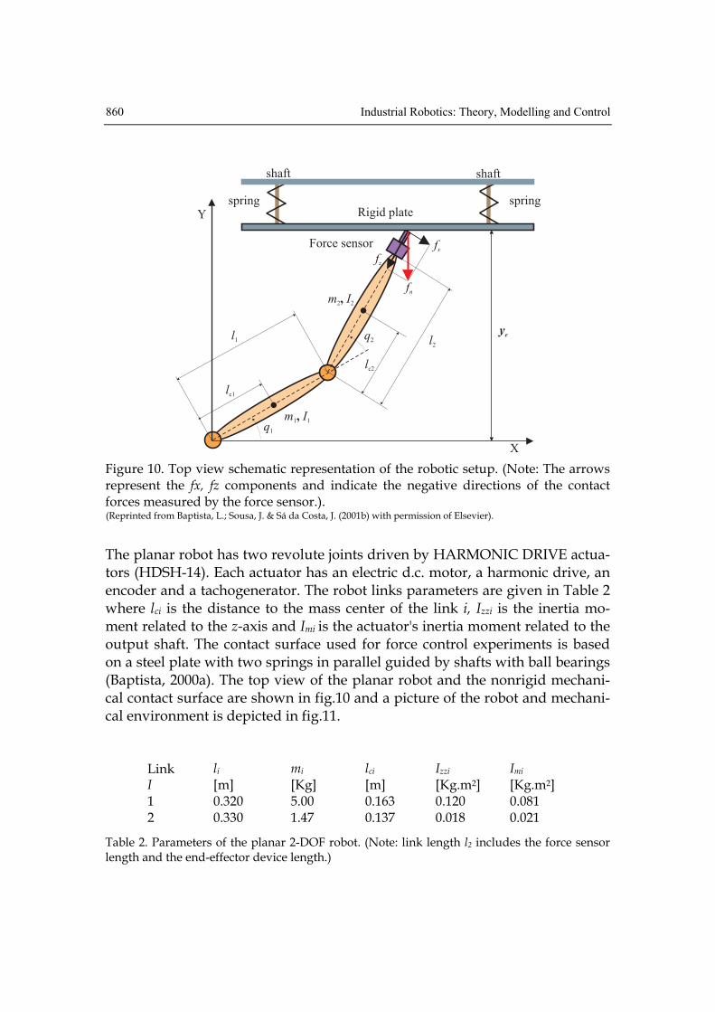
Figure 10. Top view schematic representation of the robotic setup. (Note: The arrows represent the fx, fz components and indicate the negative directions of the contact forces measured by the force sensor.). (Reprinted from Baptista, L.; Sousa, J. & Sá da Costa, J. (2001b) with permission of Elsevier).

The planar robot has two revolute joints driven by HARMONIC DRIVE actua-tors (HDSH-14). Each actuator has an electric d.c. motor, a harmonic drive, an encoder and a tachogenerator. The robot links parameters are given in Table 2 where lci is the distance to the mass center of the link i, Izzi is the inertia mo-ment related to the z-axis and Imi is the actuator's inertia moment related to the output shaft. The contact surface used for force control experiments is based on a steel plate with two springs in parallel guided by shafts with ball bearings (Baptista, 2000a). The top view of the planar robot and the nonrigid mechani-cal contact surface are shown in fig.10 and a picture of the robot and mechani-cal environment is depicted in fig.11.

Link I

li [m]

mi [Kg]

lci [m]

Izzi [Kg.m2]

Imi [Kg.m2]

1 0.320 5.00 0.163 0.120 0.081 2 0.330 1.47 0.137 0.018 0.021

Table 2. Parameters of the planar 2-DOF robot. (Note: link length l2 includes the force sensor length and the end-effector device length.)


Figure 11. Top view of the 2-DOF robot and the nonrigid mechanical environment. (Reprinted from Baptista, L.; Sousa, J. & Sá da Costa, J. (2001b) with permission of Elsevier).

6.1 Control hardware and software tools

The control hardware is based on a PC Pentium 200 MHz, a servo-axis I/O card, linear power amplifiers and a 6-axis force/torque sensor. The power am-plifiers are configured to operate as current amplifiers. In this functioning mode, the input control signal is a voltage in the range ± 10 V with current rat-ings in the interval [-2; 2] A. The signals are processed through a low cost ISA-bus servo I/O card from ServoToGo, Inc. The contact forces are measured by a JR3 6-axis force/torque sensor mounted at the end-effector of the arm. The force and torque signals are computed by a ISA-bus DSP card with a frequency rate of 8 KHz. Note that in order to reduce the surface friction during motion, a ball bearing is mounted at the end-effector contact device. The simplified con-trol hardware architecture is shown in fig.12. The real-time software tool used to implement the force control experiments was developed in the C++ language for the MS-DOS operating system. Real-time performance is guaranteed by reprogramming the Programmable Interval Timer (PIT) of the computer system (Baptista, 2000a). The periodic interrupt generated by the servo-axis I/O board PIT is configured to the Interrupt Re-quest 5 (IRQ 5), which activates the Interrupt Service Routine 13 (ISR 13). This ISR is reserved for the control algorithm implementation at a sampling fre-quency Fs=1 KHz. The software uses also the ISR 8 which is activated by the computer's IRQ 0.


AmplifierJoint 2

ServoToGo axis board JR3 DSP sensor board

ComputerPentium 200MHz

ISA BUS

Channel 0 Channel 1

Amplifier Joint 1

q

q

JR3 sensor

Figure 12. Simplified hardware control architecture of the 2-DOF robot.

This ISR is redefined to execute the safety routine at a frequency that is the double of the sampling frequency. In order to avoid the accumulation of inter-rupt requests, the ISR 13 increments a flag at the beginning of the execution of the selected control routine. This flag is decremented at the end of the execu-tion of the procedure and is checked by the safety routine, which aborts the real-time procedure if its content is superior to the unit value. In this situation, the failure is reported to the operator by the interface program.

6.2 Real-time force control algorithms

For real-time implementation of the force control algorithms presented in pre-vious sections, some simplifications were considered due to the higher number of calculations that must be performed in real-time. Let's first consider the


classical model-based impedance controller, derived from (2) and (5), repre-sented by the following equation:

( )1( ( )) ( , ) ( )Tx d d d e x x eJ M u M B e K e f C x x x g x fτ −= + + − + + +& & & (31)

It is possible to obtain an important simplification considering that Md=Mx. Moreover, it is also possible to consider ``quasi-static" conditions, which means that velocities x ≈& 0 and q ≈& 0. This is a reasonable approximation since force control tasks are generally executed at low speeds. Thus, the following simpli-fied impedance control law is obtained:

( )( ) ( )Td dJ q B e K e g qτ = + +& (32)

This control scheme is equivalent to a proportional-derivative cartesian posi-tion control law with gravity compensation. It is possible to demonstrate that for a constant reference xd and without contact with the environment, asymp-totic stability of xd is obtained (de Witt et al, 1997). This control law can be used to apply a desired contact force on the environment considering the virtual references given by the target vector [ ]Tt v dx x x= . The application of this vec-tor in the control law (32), allows a force tracking capability without explicit knowledge of the environment stiffness coefficient. In order to improve the force tracking accuracy, an integral control action can be included in (32), which leads to:

( )( ) ( )Td d i fJ q B e K e K e dt g qτ = + + +∫& (33)

where te x x= − and te x x= −& & & are redefined as virtual position and velocity er-rors and f d ee f f= − are the force errors. Taking the previous assumptions in consideration, the impedance control algorithm with force tracking imple-mented in real-time is given by (33) where the gravitational terms g(q) are null since the robot is of planar type. The main steps of the controller implementa-tion for each sampling period Ts are (Baptista et al., 2001b): • Step 1: calculation of cartesian positions and velocities, x(k) and x( k )& ,

respectively. • Step 2: calculation of the normal contact force fn(k) from JR3 sensor data. • Step 3: calculation of xv(k) in the constrained direction (y-axis):


1 if 0

1 if 0

dv n

dv

d f fv n

e

f ( k )x ( k ) f ( k )k

x ( k )f ( k ) e ( k )

x ( k ) f ( k )k̂

δ

δ κ

⎧ − − ≥⎪⎪= ⎨ +⎪ − − <⎪⎩

(34)

where

1d d df ( k ) f ( k ) f ( k )δ = − − (35) f d ne ( k ) f ( k ) f ( k )= − (36)

• Step 4: definition of the virtual vector

-axis direction -axis direction

dv

v

x ( k ) xx ( k )

x ( k ) y⎧

= ⎨ ⊥⎩

(37)

• Step 5: calculation of the control actions in the Cartesian space:

( )d d i s pf ( k ) B x( k ) K e( k ) K T I ( k )= − + +& (38) where

12p

e( k ) e( k )I ( k ) + −= (39)

• Step 6: calculation of the joint control actions

T( k ) J( q( k )) f ( k )τ = (40) Notice that in (35) the minus signals follow the convention of signals used by the force/torque sensor. In this algorithm, an estimate of the environment stiffness ek̂ is used to compute xv(k). The term f fe ( k )κ is used to compensate geometric and stiffness uncertainties and other non-modeled terms of the envi-ronment. For purposes of performance analysis, the classical hybrid position/force con-trol algorithm was also implemented in real-time. This algorithm has been pro-posed by (Raibert & Craig, 1981) and uses a selection matrix

diag with 1jS ( s ) j ,...,m= = , to separate the position and force subspaces, by the attribution of ``1" to the force subspace and ``0" to the position subspace. The matrix S is used to represent the force controlled direction and the matrix I-S to represent the remaining position controlled directions, where I is the iden-


tity matrix. In this algorithm, the control forces are given by:

[ ]1f pf ( k ) Sf ( k ) S f ( k )= + − (41) The real-time implementation of the control laws for unconstrained space and constrained space, are respectively given by:

Force subspacePosition subspace

d Pf s f I f Df

P s I p D

f ( k ) K e( k ) T K I ( k ) K xf ( k )

K e( k ) T K I ( k ) K x+ + −⎧

= ⎨ + −⎩

&

& (42)

where ef is defined in (37) and Ip follows the definition in (39) for the uncon-strained direction. The coefficients KP, KI and KD are the parameters of the PID position controller and KPf, KIf and KDf are the parameters of the PID force con-troller. Notice that velocity damping is included in the control law for the con-strained direction (Mandal & Payandeh, 1995). Unfortunately, the control scheme presented in fig.4 is not possible to imple-ment directly in real-time due to the high sampling rate used in the force con-trol loop (Fs=1 KHz). Thus, one possible solution is to use more powerful hardware and software tools to implement the control scheme in a straight-forward way. Due to computer hardware limitations, an alternative strategy was used to implement the proposed force control algorithm in real-time. The optimized virtual trajectory xv for the impedance controller is computed off-line in Matlab/Simulink using a realist simulator of the experimental robotic setup. The optimized virtual trajectory calculated off-line with an additional term for compensation of uncertainties and modeling errors is then furnished as a reference signal (xvopt) to the impedance controller described in Section 3. The virtual reference used in the simplified version of the MPA with fuzzy scaling implemented in real-time is then given by:

fv vopt f

e

e ( k )x ( k ) x ( k )

k̂κ= + (43)

where and f ek̂κ are terms as defined in (34).


7. Experimental results

In this section, experimental results obtained with the predictive force algo-rithm with fuzzy scaling proposed in this paper are presented. These results are compared with the classical force control algorithms, namely the classical impedance controller and the hybrid position/force controller. Note that the predictive control algorithm uses a nonlinear model of the nonrigid environ-ment where the stiffness coefficient is varying with the penetration depth δx. It is necessary to obtain an estimate of the environment stiffness in the con-strained direction ek̂ , which is used in (34) and (43). This estimate is obtained experimentally by measuring the linear surface displacement when a force profile is applied by the end-effector. The collected pairs of nf xδ− data are then used to estimate the global stiffness coefficient ek̂ =1636 N/m, using the least-squares method. The obtained results presented in fig.13, exhibit a large deformation of the surface when a 10 N smooth step force profile is applied on the surface. From the plot is possible to observe that the environment has a nonlinear behavior of hysteresis type (Baptista et al., 2001b). The control algorithms are implemented in the cartesian space with a sampling period of Ts = 1 ms. The implemented force/position task is a linear trajectory with 100 mm length between xi = 229.5 mm and xf = 329.5 mm along x-axis, with simultaneous application of a smooth 10 N step force profile along the y-axis, during 8 seconds. It is assumed that the arm is initially in contact with the environment. Moreover, geometric uncertainty in the contact surface of 5 mm at the end of the trajectory is intentionally imposed to the environment. The fil-tered force data components (fx, fz) are obtained from the JR3 DSP board con-sidering a first order low-pass digital filter with 500 Hz cut-off frequency in order to attenuate the force sensor noise. The predictive force control algo-rithm, which derives the virtual position to the impedance controller, use the parameters Hc= Hp = 2. As refereed in Section 4, the fuzzy scaling machine is applied only during the constant path of the reference force profile.


0 1 2 3 4 5 6−5

0

5

10

15

δx [mm]

f n [

N]

0 1 2 3 4 5 6 7 8−15

−10

−5

0

5

time [s]

f n ;

f* n [N

]

Figure 13. Estimated environment stiffness and contact forces. (Note: dashdot - esti-mated contact force n e

ˆ ˆf k xδ= ; solid - actual force fn). (Reprinted from Baptista, L.; Sousa, J. & Sá da Costa, J. (2001b) with permission of Elsevier).

The maximum allowed increments Δxv at each time step are the following (in mm):

2 20 75 10 0 0 75 10* . .Ω − −⎡ ⎤= − × ×⎣ ⎦ (44) The impedance control algorithm use the parameters presented in Table 3 for the real-time control experiments. The force compensation gain is set to fκ =0.025, and was selected from experimental trials.

Axis Kd Ki Bd x-axis 3000 4000 6 y-axis 2000 3000 2

Table 3. Impedance control parameters. Figure 14 presents the end-effector’s position in the x-y axis coordinates using the real-time implementation of the predictive force control algorithm with fuzzy scaling. For the same controller, the optimized virtual position given by (43) and the actual contact force are presented in fig.15. Figure 16 presents the obtained position and force errors. The experimental results obtained with the classical impedance controller are presented in fig. 17, where the position and


force errors are depicted. The parameters for the hybrid position/force control-ler used in the real-time tests are presented in Table 4 and the position and force errors are depicted in fig.18.

Axis KP KI KD x-axis 3000 4000 6 y-axis 570 2500 2

Table 4. Parameters of the hybrid position/force controller. The results presented for the predictive force control algorithm reveal an accu-rate force tracking accuracy when compared to the equivalent results obtained with the impedance and hybrid control algorithms. The proposed controller exhibit significantly better results, especially during the time-varying force ref-erence trajectory. The impedance controller with force tracking reveal some difficulties in following the force reference path when this is not constant. The force control performance of the hybrid controller drops significantly during the final part of the trajectory due to the geometric uncertainty, which is not ef-ficiently compensated by the algorithm.

0 1 2 3 4 5 6 7 8220

240

260

280

300

320

340

x d ;

x [m

m]

0 1 2 3 4 5 6 7 8440

442

444

446

448

450

time [s]

y [m

m]

Figure 14. Predictive force control algorithm with fuzzy scaling: X-axis position coor-dinate, Y-axis constrained position coordinate. (Reprinted from Baptista, L.; Sousa, J. & Sá da Costa, J. (2001b) with permission of Elsevier).


0 1 2 3 4 5 6 7 8440

442

444

446

448

450

x v [

mm

]

0 1 2 3 4 5 6 7 8−15

−10

−5

0

5

time [s]

f d ;

f n [

N]

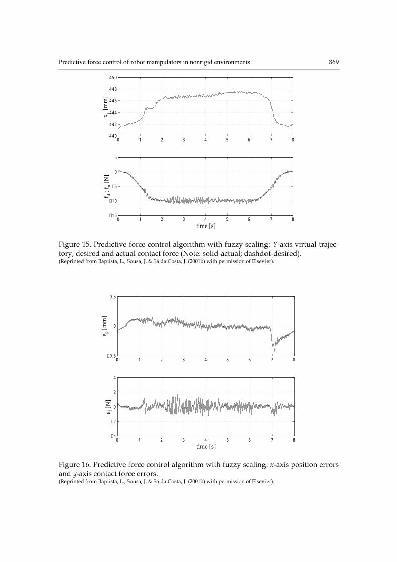
Figure 15. Predictive force control algorithm with fuzzy scaling: Y-axis virtual trajec-tory, desired and actual contact force (Note: solid-actual; dashdot-desired). (Reprinted from Baptista, L.; Sousa, J. & Sá da Costa, J. (2001b) with permission of Elsevier).

0 1 2 3 4 5 6 7 8−0.5

0

0.5

e p [

mm

]

0 1 2 3 4 5 6 7 8−4

−2

0

2

4

time [s]

e f [

N]

Figure 16. Predictive force control algorithm with fuzzy scaling: x-axis position errors and y-axis contact force errors. (Reprinted from Baptista, L.; Sousa, J. & Sá da Costa, J. (2001b) with permission of Elsevier).


0 1 2 3 4 5 6 7 8−0.5

0

0.5

e p [

mm

]

0 1 2 3 4 5 6 7 8−4

−2

0

2

4

time [s]

e f [

N]

Figure 17. Impedance control with force tracking: x-axis position errors and y-axis contact force errors. (Reprinted from Baptista, L.; Sousa, J. & Sá da Costa, J. (2001b) with permission of Elsevier).

In order to compare the performance of the controllers, the Euclidian norm ( . ) of position and force errors and the absolute maximum error values for the given task are presented in Table 5.

Force controllers pe

[m]

Max(ep)

[mm] fe

[N]

Max(ef)

[N] Hybrid position/force control 8.1 0.43 63.89 2.76 Impedance control with force tracking 8.5 0.49 50.63 2.33 Predictive force control with fuzzy scaling

8.1 0.42 37.40 1.73

Table 5. Euclidian norm of position, force errors and absolute maximum errors.

From Table 4 results, is possible to conclude that predictive force control algo-rithm proposed in this paper reduces the norm of the force error in 26% when compared to the impedance controller with force tracking, which is a quite significant value. The reduction in the norm of the force error is even more significant when compared to the hybrid position/force controller results (41%). The experimental results reveal the successful implementation of the proposed predictive force control strategy in real-time, in the presence of non-rigid environments with uncertainties.


0 1 2 3 4 5 6 7 8−0.5

0

0.5

e p [

mm

]

0 1 2 3 4 5 6 7 8−4

−2

0

2

4

time [s]

e f [

N]

Figure 18. Hybrid position/force control: x-axis position errors and y-axis contact force errors. (Reprinted from Baptista, L.; Sousa, J. & Sá da Costa, J. (2001b) with permission of Elsevier).

8. Conclusion

In this article, a force control scheme integrating a model predictive algorithm and an impedance controller in the presence of nonrigid environments is pro-posed. The force controller uses a MPA with a fuzzy scaling machine to allevi-ate the problems introduced by the discretization of inputs required by the B&B algorithm. The optimization procedure is nonconvex since a nonlinear model of the environment is considered. Simulation results were carried out considering a 2-DOF robot model interacting with a nonrigid environment with nonlinear characteristics. A real-time implementation of the fuzzy predic-tive algorithm is derived, which uses an optimal virtual trajectory computed off-line. The experimental results are compared to other classical force control techniques, which are the impedance control with force tracking and the hy-brid position/force control. Simulation and experimental results reveal that the proposed MPA with fuzzy scaling force controller presents a significant better force tracking performance when compared to the conventional force controllers. Future research will concentrate on the on-line implementation of the full ver-sion of the fuzzy predictive force control algorithm and the extension of the control scheme to a robot with more than two joints.


AKNOWLEDGMENTS

Part of the material in this chapter appeared in various journal and conference publications. These publications are referred to in the relevant paragraphs, and they are listed in the bibliography. The material, including figures and tables, is reproduced with the kind permission of the respective copyright holders. The list of the copyright holders is as follows: Springer Science and Business Media: Baptista, L.; Sousa, J. & Sá da Costa, J. (2001a). Elsevier Science: Bap-tista, L.; Sousa, J. & Sá da Costa, J. (2001b).

9. References

Baptista, L.; (2000a). Adaptive force and position control of robot manipulators, PhD Thesis, Technical University of Lisbon, Mechanical Engineering De-partment, Lisbon (in portuguese)

Baptista,L; Ayala Botto, M. & Sá da Costa, J. (2000b). A predictive force control approach of robot manipulators in nonrigid environments. International Journal of Robotics and Automation, 15(2) pp.94-102, ISSN 0826-8185

Baptista,L; Sousa, J. & Sá da Costa, J. (2001a). Force control of robot manipula-tors using a fuzzy predictive approach. Journal of Intelligent and Robotic Systems, 30(4), April 2001, pp.359-376, ISSN 0921-0296

Baptista,L; Sousa, J. & Sá da Costa, J. (2001b). Force predictive algorithms ap-plied to real-time force control. Control Engineering Practice, 9(4), pp.411-423, ISSN 0967-0661

Corbet, T. ; Sepehri, N. & Lawrence, P. (1996). Fuzzy control of a class of hy-draulically actuated industrial robots. IEEE Transactions Control Systems Technology, 4(4), pp.419-426

De Witt, C. ; Siciliano, B. & Bastin, G. (1997). Theory of robot control. Springer-Verlag, ISBN 3-540-76054-7, London, UK

De Schutter, J. ; Bruyninckx, H. & Spong, M. (1997). Force control: a bird’s eye. Proceedings of IEEE CSS/RAS International Workshop on Control Problems in Robotics and Automation: Future directions. San Diego, December 1997, USA

Economou, C. ; Morari, M. & Palsson, B. (1986). Internal model control. 5. Exten-sion to nonlinear systems. Industrial Engineering Chemical Process De-sign and Development, 25, American Chemical Society, pp.404-411

Hogan, N. (1985). Impedance control: An approach to manipulation: Part I-II-III. Journal of Dynamic Systems, Measurement and Control, 107(1), pp.1-24

Jaritz, A. & Spong, M. (1996). An experimental comparison of robust control algorithms on a direct drive manipulator. IEEE Transactions on Control Systems Technology, 4, pp.614-626


Jung, S. & Hsia, T. (1995). On neural network application to robust impedance control of robot manipulators. Proceedings of the IEEE International Con-ference on Robotics and Automation, pp. 869-874

Lin, S. & Huang, A. (1997). Position-based fuzzy force control for dual indus-trial robots. Journal of Intelligent and Robotic Systems, 19, pp.393-409

Liu, M. (1995). Force-controlled-fuzzy-logic-based robotic deburring. Control Engineering Practice, 3(2), pp.189-201, ISSN 0967-0661

Love, L. & Book, W. (1995). Environment estimation for enhanced impedance control. Proceedings of the IEEE International Conference on Robotics and Automation, pp. 1854-1859

Kieffer, J. & Yu, K. (1999). Robotic force/velocity control for following un-known contours of granular materials. Control Engineering Practice, 7(10), October 1999, pp.1249-1256, ISSN 0967-0661

Klir, G. & Yuan, B. (1995). Fuzzy set and fuzzy logic: theory and applications, Englewood Cliffs, Prentice Hall, ISBN 0792377338, NJ

Maciejowski, J. (2002). Predictive control with constraints, Prentice Hall Inc., New York, USA, ISBN 0201398230

Marhefka, D. & Orin, D. (1996). Simulation of contact using a nonlinear damp-ing model. Proceedings of the IEEE International Conference on Robotics and Automation, pp.1662-1668

Mandal, N. & Payandeh, S. (1995). Control strategies for robotic control tasks: an experimental study. Journal of Robotic Systems, 12(1), pp.67-92

Raibert, M & Craig, J. (1981). Hybrid position/force control of manipulators. Journal of Dynamic Systems, Measurement and Control, 102(2), pp.126-133

Siciliano, B. & Villani, L. (2000). Robot force control, Springer-Verlag, New York, ISBN 0792377338

Singh, S, & Popa, D. (1995). An analysis of some fundamental problems in adaptive control of force and impedance behavior: theory and experi-ments. IEEE Transactions on Robotics and Automation, 11, pp.912-921

Sousa, J. ; Babuska, R. & Verbruggen, H. (1997). Branch-and-bound optimiza-tion in fuzzy predictive control: an application to an air conditioning system. Control Engineering Practice, 5(10), October 1997, pp.1395-1406, ISSN 0967-0661

Sousa, J. & Setnes, M. (1999). Fuzzy predictive filters in model predictive con-trol. IEEE Transactions on Industrial Electronics, 46(6), December 1999, pp.1225-1232

Volpe, R. & Khosla, P. (1995). On the equivalence of second order impedance control and proportional gain explicit force control. International Journal of Robotics Research, 14(6), pp.574-589

Yao, B. & Tomizuka, M. (1995). Adaptive control of robot manipulators in con-strained motion – controller design. Journal of Dynamic Systems, Meas-urement and Control, 117, pp.320-328


Wada, H. ; Fukuda, T. ; Kosuge, K. ; Arai, F. & Watanabe, K. (1993). Damping control with consideration of dynamics of the environment. Proceedings of the International Conference on Intelligent Robots and Systems, 1, pp.1516-1520

Zeng, G. & Hemami, A. (1997). An overview of robot force control. Robotica, 15(5), pp.473-482

Documents

Predictive Force Control of Robot Manipulators in … force control of robot manipulators in nonrigid environments 843 lis effects, as well as geometric and stiffness uncertainties