Predictive Control for the Grape Juice Concentration Processcdn.intechweb.org/pdfs/29695.pdf · · 2012-07-0390 Frontiers of Model Predictive Control The type and magnitude of degradation

5

Predictive Control for the Grape Juice Concentration Process

Graciela Suarez Segali1 and Nelson Aros Oñate2 1Department of Chemical Engineering, Faculty of Engineering,

National University of San Juan, Avda. Libertador San Martín, San Juan,

2Department of Electrical Engineering, Faculty of Engineering, University of La Frontera, Avda. Francisco Salazar, Temuco,

1Argentina 2Chile

1. Introduction

Concentrated clear grape juices are extensively used in the enological industry. Their use as constituents of juices, jellies, marmalades, jams, colas, beverages, etc., generates a consumer market with an increasing demand because they are natural products with an industrial versatility that allows them to compete with other fruit juices.

Argentina is one of the principal producers and exporters of concentrated clear grape juices in the world. They are produced mainly in the provinces of Mendoza and San Juan (Argentine Republic) from the virgin grape juice and in the most part from sulfited grape juices. The province of Mendoza’s legislation establishes that a portion of the grapes must be used for making concentrated clear grape juices. This product has reached a high level of penetration in the export market and constitutes an important and growing productive alternative.

An adequate manufacturing process, a correct design of the concentrate plants and an appropriate evaluation of their performance will facilitate optimization of the concentrated juices quality parameters (Pilati, 1998; Rubio, 1998). The plant efficiency is obtained from knowledge of the physics properties of the raw material and products (Moressi, 1984; Piva, 2008). These properties are fundamental parameters that are used in the designing and calculations on all the equipment used and also in the control process.

The juices (concentrate and intermediate products) physical properties, such as density, viscosity, boiling point elevation, specific heat and coefficient of thermal expansion, are affected by their solid content and their temperature (Schwartz, 1986). For this reason, it is necessary to know the physical properties values, as a function of the temperature and the solids content, during the manufacture process, not just to obtain an excellent quality, but also to develop a data base, that is essential for optimizing the installation design and the transformation process itself. The principal solids constituents of clear grape juices are sugars (mostly glucose and fructose) and its concentration affects directly the density, viscosity and refraction index.

www.intechopen.com

Frontiers of Model Predictive Control 90

The type and magnitude of degradation products will depend on the starting reagent condition (Gogus, et al., 1998). Acetic, formic, and D/L-lactic acids were identified at the end of thermal degradation of sugar solutions (Asghari and Yoshida, 2006), and a reaction scheme was proposed by Ginz et al. (2000). Sugar degradation may result in browning of solutions with polymeric compounds as the ultimate product of degradation, generally known as “melanoidins”, involving the formation of 5-(hydroxymethyl)-2-furancarboxaldehyde (5-HMF) as intermediate.

Barbieri and Rossi (1980) worked with white concentrated clear grape juice in a falling film multiple effect evaporators. They obtained 18.2, 27.3, 38.6, 48.6 and 64.6 °Brix samples. They measured density, viscosity and boiling point elevation as a function of soluble solids concentration and temperature. They presented the results in plots with predictive equations for the properties studied.

Di Leo (1988) published density, refraction index and viscosity data for a rectified concentrated grape juice and an aqueous solution of a 1:1 glucose/levulose mixture, for a soluble solids concentrate range from 60 to 71% (in increments of 0.1%) and 20 °C. The author determinated the density in undiluted and 2.5-fold diluted samples (100 g of clear grape juice in 250 ml of solution at 20 °C), finding different results between both determinations. He recommended measuring density without dilution.

Pandolfi et al., (1991) studied physical and chemical characteristics of grape juices produced in Mendoza and San Juan provinces, Argentina. They determined density at 20°C in sulfited grape juices of 20–22°Bx and concentrated grape juices of 68–72°Bx. They obtained no information on intermediate concentrations or other temperatures. In general, the clarified juice concentrates have a Newtonian behavior (Ibarz & Ortiz, 1993; Rao, Cooley & Vitali, 1984; Sáenz & Costell, 1986; Saravacos, 1970).

Numerous industrial processes are multivariable systems which require a large number of variables to be controlled simultaneously (Kam, 1999; Kam, 2000). The controller design is for this type of system has a great interest in control theory (Doyle, 1979; Freudenberg, 1988; Friedland, 1989; Middleton, 1990; Zang, 1990; Aros, 2008; Suarez, 2010). This work presents an interactive tool to facilitate understanding of the control of multivariable systems (MIMO) using the technique of Generalized Predictive Control (GPC). The tool can handle the main concepts of predictive control with constraints and work both as monovariable and multivariable systems.

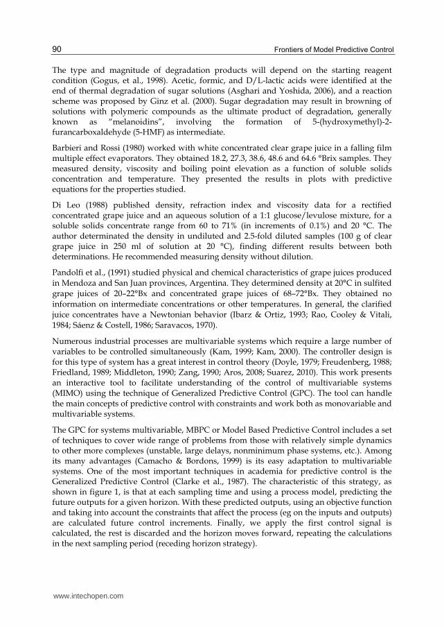
The GPC for systems multivariable, MBPC or Model Based Predictive Control includes a set of techniques to cover wide range of problems from those with relatively simple dynamics to other more complexes (unstable, large delays, nonminimum phase systems, etc.). Among its many advantages (Camacho & Bordons, 1999) is its easy adaptation to multivariable systems. One of the most important techniques in academia for predictive control is the Generalized Predictive Control (Clarke et al., 1987). The characteristic of this strategy, as shown in figure 1, is that at each sampling time and using a process model, predicting the future outputs for a given horizon. With these predicted outputs, using an objective function and taking into account the constraints that affect the process (eg on the inputs and outputs) are calculated future control increments. Finally, we apply the first control signal is calculated, the rest is discarded and the horizon moves forward, repeating the calculations in the next sampling period (receding horizon strategy).

www.intechopen.com

Predictive Control for the Grape Juice Concentration Process 91

Fig. 1. MBPC action.

The GPC technique is based on the use of models derived from transfer functions (transfer matrices in the multivariate case). The use of a formulation of this kind against an internal description has certain advantages in the field of development of interactive tools. The transfer function formulation is more intuitive, being based only on information input and output measurable and arrange its elements (poles and zeros) of a clear physical meaning and interpretation.

This is critical in the design of interactive tools, which simultaneously shows different representations of the system that allow to analyze how the change affects any parameter of the plant-controller-model global behavior of the controlled system without ever losing its physical sense, allowing to develop their intuition and skills.

The basic idea was proposed of GPC is to calculate a sequence of future control signals in such a way that it minimizes a multistage cost function defined over a prediction horizon. The index to be optimized is the expectation of a quadratic function measuring the distance between the predicted systems output and some predicted reference sequence over the horizon plus a quadratic function measuring the control effort. This approach was used in Lelic & Wellstead (1987) and Lelic & Zarrop (1987), to obtain a generalized pole placement controller which is an extension of the well-known pole placement controllers Allidina & Hughes (1980) and belongs to the class of extended horizon controllers.

Generalized Predictive Control has many ideas in common with the predictive controllers previously mentioned since it is based upon the same concepts but it has some differences. As will be seen, it provides an analytical solution (in the absence of constraints)nit can deal with unstable and nonminimum phase plants and it incorporates the concept of control horizon as well as the consideration of weighting control increments in the cost function. The general set of choices available for GPC leads to a greater variety of control objectives compared to other approaches, some of which can be considered as subsets or limiting cases of GPC. In particular, the strategy GPC uses the model CARIMA (Controlled Auto Regressive Integrated Moving Average) to predict the process output.

2. Process description

Figure 2 show the input and output streams in a vertical generic effect evaporator with long tubes. The solution to be concentrated circulates inside the tubes, while the steam, used to heat the solution, circulates inside the shell around the tubes.

www.intechopen.com


The evaporator operates in co-current. The solution to be concentrated and the steam are fed to the first effect by the bottom and by the upper section of the shell, respectively. Later on, the concentrated solution from the first effect is pumped to the bottom of the second effect, and so on until the fourth effect. On the other hand, the vapor from each effect serves as heater in the next one. Finally, the solution leaving the fourth effect attains the desired concentration.

Each effect has a baffle in the upper section that serves as a drops splitter for the solution dragged by the vapor. The vapor from the fourth effect is sent to a condenser and leaves the process as a liquid. The concentrated solution coming from the fourth effect is sent to a storage tank.

Fig. 2. Photo of evaporator and scheme of effect i in the four-stage evaporator flow sheet. 件噺な, ⋯ ,4. 3. Phenomenological model

Stefanov & Hoo (2003) have developed a rigorous model with distributed parameters based on partial differential equations for a falling-film evaporator, in which the open-loop stability of the model to disturbances is verified. On the other hand, various methods have been proposed in order to obtain reduced-order models to solve such problems (Christofides, 1998; El-Farra, Armaou and Christofides, 2002; Hoo and Zheng, 2001; Zheng and Hoo, 2002). However, the models are not a general framework yet, which assure an effective implementation of a control strategy in a multiple effect evaporator.

In practice, due to a lack of measurements to characterize the distributed nature of the process and actuators to implement such a solution, the control of systems represented by partial differential equation (PDE) in the grape juice evaporator, is carried out neglecting the spatial variation of parameters and applying lumped systems methods. However, a

www.intechopen.com


distributed parameters model must be developed in order to be used as a real plant to test advance control strategies by simulation.

In this work, it is used the mathematical model of the evaporator developed by Ortiz et al.

(2006), which is constituted by mass and energy balances in each effect. The assumptions are: the main variables in the gas phase have a very fast dynamical behavior, therefore the corresponding energy and mass balances are not considered. Heat losses to surroundings are neglected and the flow regime inside each effect is considered as completely mixed.

a. Global mass balances in each effect:

ii si i

dWW W W

dt1 (1)

in this equations iW i, 1,..., 4 are the solution mass flow rates leaving the effects 1 to 4, respectively. W0 is the input mass flow rate that is fed to the equipment. siW i, 1,..., 4 are the vapor mass flow rates coming from effects 1 to 4, respectively. dMi dt i/ , 1,..., 4represent the solution mass variation with the time for each effect.

b. Solute mass balances for each effect:

i ii i i i

d W XW X W X

dt1 1

( ) (2)

where, iX i, 1,..., 4 are the concentrations of the solutions that leave the effects 1 to 4, respectively. is the concentration of the fed solution.

c. Energy balances:

i ii i i i si si i i si i

dW hW h W h W H A U T T

dt1 1 1( ) (3)

where, ih i, 1,..., 4 are the liquid stream enthalpies that leave the corresponding effects, h0 is the feed solution enthalpy, and siH i, 1,..., 4 are the vapor stream enthalpies that leave the corresponding effects and, iA represents the heat transfer area in each effect. The model also includes algeb raic equations. The vapor flow rates for each effect are calculated neglecting the following terms: energy accumulation and the heat conduction across the tubes. Therefore:

i i si isi

si ci

U A T TW

H h1

1

( )

(4)

For each effect, the enthalpy can be estimated as a function of temperatures and concentrations (Perry, 1997). Them:

si siH T2509.2888 1.6747 (5)

ci sih T4.1868 (6)

,oX

www.intechopen.com


pi i iC X T3 40.80839 4.3416 10 5.6063 10 (7)

i i i i ih T X T T3 4 20.80839 4.316 10 2.80315 10 (8)

iT i, 1,..., 4 are the solution temperatures in each effect, and sT 0 , is the vapor temperature that enters to the first effect. siT i, 1,..., 4 are the vapor temperatures that leave each effect.

The heat transfer coefficients are:

JL

sii

i i

D WU

T

0.57 3.6

0.25 0.1

490.

(9)

Once viscosity values were established at different temperatures, (apparent) flow Activation Energy values for each studied concentration were calculated using the Arrhenius equation:

航噺航著exp岫伐帳尼眺脹岻 (10)

航著噺伐exp岫欠待髪欠怠稽堅件捲髪欠態稽堅件捲態 (11)

継銚劇斑噺伐exp岫欠待髪欠怠稽堅件捲髪欠態稽堅件捲態 (12)

The global heat-transfer coefficients are directly influenced by the viscosity and indirectly by the temperature and concentration in each effect. The constants 欠待, 欠怠 y 欠態 depend on the type of product to be concentrated (Kaya, 2002; Perry, 1997; Zuritz, 2005).

Although the model could be improved, the accuracy achieved is enough to incorporate a control structure.

4. Standard model predictive control

The biggest problem that arises in the implementation of conventional PID controllers, arises when there are high nonlinearities and long delays, a possible solution to these arises with the implementation of predictive controllers, in which the entry in a given time (t) will generate an output at a time (t +1), using a control action at time t.

The model-based predictive control is currently presented as an attractive management tool for incorporating operational criteria through the use of an objective function and constraints for the calculation of control actions. Furthermore, these control strategies have reached a significant level of acceptability in practical applications of industrial process control.

The model-based predictive control is mainly based on the following elements:

The use of a mathematical model of the process used to predict the future evolution of the controlled variables over a prediction horizon.

The imposition of a structure in the future manipulated variables. The establishment of a future desired trajectory, or reference to the controlled variables. The calculations of the manipulated variables optimizing a certain objective function or

cost function. The application of control following a policy of moving horizon.

www.intechopen.com


4.1 Generalized predictive control

The CARIMA model of the process is given by:

畦岫権貸怠岻検岫建岻噺稽岫権貸怠岻憲岫建伐な岻髪怠∆ 系岫権貸怠岻結岫建岻 (13)

with ∆噺な伐権貸怠

And the C polynomial is chosen to be 1, from what they if C-1 can be truncated it can be absorbed into A and B.

The GPC algorithm consists of applying a sequence that minimizes a multistage cost function of the form

蛍岫軽怠, 軽態, 軽通岻噺 ∑ 絞岫倹岻岷検賦岫建髪倹|建岻伐拳岫建髪倹岻峅態髪 ∑ 膏岫倹岻岷Δ憲岫建髪倹伐な岻峅態朝迭珍退怠朝鉄珍退朝迭 (14)

where: 検賦岫建髪倹|建岻 is a sequence of (j) best predictions from the output of the system later instantly t and performed with the known data to instantly t. Δ憲岫建髪倹伐な岻 is a sequence control signal increases to come, to be obtained from the minimization of the cost function.

N1, N2 and Nu are the minimum and maximum costing horizons, and control horizon. N1 and N2 That does not necessarily coincide with the maximum prediction horizon. The meaning of them is quite intuitive, they mark the limits of the moments that criminalizes the discrepancy of the output with the reference.

δ(j) and ┣(j) are weighting factors they are sequences are respectively weighted tracking errors and future control efforts. Usually considered constant values or exponential sequences. These values can be used as tuning parameters.

Reference trajectory: one of the benefits of predictive control is that if you know a priori the future evolution of the reference, the system can start to react before the change is actually carried out, avoiding the effects of the delay in the response of the process. On the criterion of minimizing (Bitmead et al., 1990), most of the methods often used a trajectory of reference w(t+j) which does not necessarily coincide with the actual reference. Normally it would be a soft approach from the current value of the output y (t) to the known reference, through a first-order dynamics.

拳岫建髪倹岻噺糠拳岫建髪倦伐な岻髪岫な伐糠岻堅岫建髪倹岻 (15)

where

α is a parameter between 0 and 1 that constitutes an adjustable value that will influence the dynamic response of the system. where α = diag( α1, α2,. . . , αn) is the diagonal soften factor matrix;

(1-α) = diag(1- α1, 1- α2,….1- αn); r(t+j) is the system’s future set point sequence. By employing this cost function, the distance between the model predictive output and the

www.intechopen.com


soften future set point sequence is minimized over the predictive horizon while the variation of the control input is preserved small over the control horizon.

In order to optimize the cost function the optimal prediction of y(t+j) for j ≥ N1 and j ≤ N2 will be obtained. Consider the following Diophane equation:

な噺継珍岫権貸怠岻畦寞岫権貸怠岻髪権貸怠繋珍岫権貸怠岻 (16)

where 畦寞岫権貸怠岻噺 Δ畦岫権貸怠岻

The polynomial Ej and Fj are uniquely defined with degrees j-1 and na, respectively. They can be obtained by dividing 1 by Ã(z-1) until the remainder can be factorized as z-1 Fj(z-1). The quotient of the division is the polynomial Ej (z-1).

畦寞岫権貸怠岻継珍岫権貸怠岻検岫建髪倹岻噺継珍岫権貸怠岻稽岫権貸怠岻∆憲岫建髪倹伐穴伐な岻髪継珍岫権貸怠岻結岫建髪倹岻 (17)

Considering the equation (16), the equation (17) can be written as 岾な伐権貸怠繋珍岫権貸怠岻峇検岫建髪倹岻噺継珍岫権貸怠岻稽岫権貸怠岻∆憲岫建髪倹伐穴伐な岻髪継珍岫権貸怠岻結岫建髪倹岻

which can be rewritten as:

検岫建髪倹岻噺繋珍岫権貸怠岻検岫建岻髪継珍岫権貸怠岻稽岫権貸怠岻∆憲岫建髪倹伐穴伐な岻髪継珍岫権貸怠岻結岫建髪倹岻 (18)

As the degree of polynomial Ej (z-1) = j-1the noise terms in equation (18) are all in the future. The best prediction of y (t+j) is therefore:

検賦岫建髪 |建岻噺罫珍岫権貸怠岻∆憲岫建髪倹伐穴伐な岻髪繋珍岫権貸怠岻検岫建岻 (19)

Where 罫珍岫権貸怠岻噺継珍岫権貸怠岻稽岫権貸怠岻

There are other ways to formulate a GPC as can be seen in Albertos & Ortega, (1989)

The polynomials Ej, Fj and Gj can be obtained recursively. 繋珍岫権貸怠岻噺繋珍,待髪繋珍,怠岫権貸怠岻髪繋珍,態岫権貸態岻髪 ⋯ 髪繋珍,津銚岫権貸津銚岻継珍岫権貸怠岻噺継珍,待髪継珍,怠岫権貸怠岻髪継珍,態岫権貸態岻髪 ⋯ 髪継珍,珍貸怠盤権貸岫珍貸怠岻匪罫珍岫権貸怠岻噺罫珍,待髪罫珍,怠岫権貸怠岻髪罫珍,態岫権貸態岻髪 ⋯ 髪罫珍,珍貸怠盤権貸岫珍貸怠岻匪

for instant j +1 繋珍袋怠岫権貸怠岻噺繋珍袋怠,待髪繋珍袋怠,怠岫権貸怠岻髪繋珍袋怠,態岫権貸態岻髪 ⋯ 髪繋珍袋怠,津銚岫権貸津銚岻継珍袋怠岫権貸怠岻噺継珍岫権貸怠岻髪継珍袋怠,珍盤権貸珍匪罫珍袋怠岫権貸怠岻噺罫珍岫権貸怠岻髪繋珍,待盤権貸珍匪稽

Consider the group of j ahead optimal prediction For a reasonable response, these bounds are assumed to be Camacho & Bordons, (2004):

N1 = d + 1

www.intechopen.com


N2 = d + N

Nu = N

検噺罫憲髪繋岫権貸怠岻髪罫嫗岫権貸怠岻∆憲岫建伐な岻 (20)

検噺琴欽欽欽欣検賦岫建髪穴髪な|建岻検賦岫建髪穴髪に|建岻..検賦岫建髪穴髪軽|建岻筋禽禽

禽禁罫噺琴欽欽

欽欣罫待ど … ど罫怠罫待 … ど..罫朝貸怠罫朝貸態罫待筋禽禽禽禁憲噺琴欽欽

欽欣 ∆憲岫建岻∆憲岫建髪な岻..∆憲岫建髪軽伐な岻筋禽禽禽禁

繋岫権貸怠岻噺琴欽欽欽欣繋鳥袋怠岫権貸怠岻繋鳥袋態岫権貸怠岻..繋鳥袋朝岫権貸怠岻筋禽禽

禽禁罫嫗岫権貸怠岻噺琴欽欽

欽欣岫罫鳥袋怠岫権貸怠岻伐罫待岻権岫罫鳥袋態岫権貸怠岻伐罫待伐罫怠権貸怠岻権態..岫罫鳥袋朝岫権貸怠岻伐罫待伐罫怠権貸怠伐 ⋯ 罫朝貸怠権貸岫朝貸怠岻権朝筋禽禽禽禁

After making some assumptions and mathematical operations the equation (14) is written:

蛍噺岫罫憲髪血伐拳岻脹岫罫憲髪血伐拳岻髪膏憲脹憲 (21)

where 血噺罫嫗岫権貸怠岻∆憲岫建伐な岻拳噺岷拳岫建髪穴髪な岻拳岫建髪穴髪に岻 … 拳岫建髪穴髪軽岻峅脹

Then (21) is

蛍噺なに憲脹茎憲髪決脹憲髪血待

with 茎噺に岫罫脹罫髪膏荊岻決脹噺に岫血伐拳岻脹罫血待噺岫血伐拳岻脹岫血伐拳岻

Many processes are affected by external disturbances caused by variation of variables that can be measured. Consider, for example, the evaporated where the first effect temperature is controlled by manipulating the steam of temperature, any variation of the steam temperature, influence the first effect temperature. These type of perturbations, also known as load disturbances, can easily be handled by the use of feedforward controllers. Known disturbances can be taken explicitly into account in MBPC, as will be seen in the following.

Consider a process described by the following in this case the CARIMA model must be changed to include the disturbances:

畦岫権貸怠岻検岫建岻噺稽岫権貸怠岻憲岫建伐な岻髪経岫権貸怠岻懸岫建岻髪怠∆ 系岫権貸怠岻結岫建岻 (22)

www.intechopen.com


Where the variable v(t) is the measured disturbance at time t and D(z-1) is a polynomial defined as: 経岫権貸怠岻噺穴待髪穴怠権貸怠髪穴態権貸態髪 ⋯ 髪穴津鳥権貸津鳥

If equation (16) is multiplied by ∆Ej (z-1) zj. 継珍岫権貸怠岻畦寞岫権貸怠岻検岫建髪倹岻噺継珍岫権貸怠岻稽岫権貸怠岻∆憲岫建髪倹伐な岻髪継珍岫権貸怠岻経岫権貸怠岻∆懸岫建髪倹岻髪継珍岫権貸怠岻結岫建髪倹岻

and manipulation these equation, we get 検岫建髪倹岻噺繋珍岫権貸怠岻検岫建岻髪継珍岫権貸怠岻稽岫権貸怠岻∆憲岫建髪倹伐な岻髪継珍岫権貸怠岻経岫権貸怠岻∆岫建髪倹岻髪継珍岫権貸怠岻結岫建髪倹岻

Notice that because the degree of Ej (z-1) is j-1, the noise terms are all in the future; by taking the expectation operator and considering that E[e(t)] = 0 the expected value for y (t+j) is given by: 検賦岫建髪倹|建岻噺継岷検岫建髪倹岻峅噺繋珍岫権貸怠岻検岫建岻髪継珍岫権貸怠岻稽岫権貸怠岻∆憲岫建髪倹伐な岻髪継珍岫権貸怠岻経岫権貸怠岻∆懸岫建髪倹岻

Whereas the polynomial Ej (z-1) D (z-1) = Hj (z-1) + z-j H’j (z-1), with δ(Hj(z-1)) = j-1, the prediction equation can be rewritten as 検賦岫建髪倹|建岻噺罫珍岫権貸怠岻∆憲岫建髪倹伐な岻髪茎珍岫権貸怠岻∆懸岫建髪倹岻髪罫珍嫗岫権貸怠岻∆憲岫建伐な岻髪茎珍嫗岫権貸怠岻∆懸岫建岻

髪繋珍岫権貸怠岻検岫建岻 (23)

Note that the last three terms of the right-hand side of this equation depend on past values of the process output, measured disturbances and input variables and correspond to the free response of the process considered if the control signals and measured disturbances are kept constant; while the first term only depends on future values of the control signals and can be interpreted as the force response, that is, the response obtained when the initial conditions are zero y(t-j) = 0, ∆u(t-j-1) = 0, ∆v(t-j) for j > 0.

The other terminus equation (23) depends on the future deterministic disturbance. 検賦岫建髪倹|建岻噺罫珍岫権貸怠岻∆憲岫建髪倹伐な岻髪茎珍岫権貸怠岻∆懸岫建髪倹岻髪血珍血珍噺罫珍嫗岫権貸怠岻∆憲岫建伐な岻髪茎珍嫗岫権貸怠岻∆懸岫建岻髪繋珍岫権貸怠岻検岫建岻

Then for N j ahead predictions: 検賦岫建髪軽|建岻噺罫朝岫権貸怠岻∆憲岫建髪軽伐な岻髪茎珍岫権貸怠岻∆懸岫建髪軽岻髪血朝

If one considers 茎珍噺 ∑ 月沈権貸怠珍沈退怠 where hi are the coefficients of system step response to the disturbance, if f’ = Hv + f.

The predictive equation of is

Y = Gu + f’

www.intechopen.com


5. Simulations results

5.1 Open loop

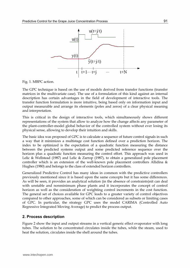
The following figures shows the behavior of each of the states against disturbances stair, rising and declining in each of the manipulated variables such as feed flow of the solution to concentrate, steam temperature, concentration of food and feed temperature. In each figure a, b, c and d correspond to 1, 2, 3 and 4 th respectively effect.

The following figure shows the response of the open loop system, when making a disturbance in one of the manipulated variables such as flow of food; in the figure 3 is represented the concentration of output in each of the effects and figure 4 is represented the temperature in each of the effects.

(a) (b)

(c) (d)

Fig. 3. Behavior of the outlet concentration of each of the effects of the evaporator to a change of a step in the flow of food (increase of 5% - decrease of 5%)

www.intechopen.com


(a) (b)

(c) (d)

Fig. 4. Behavior of the temperature in the evaporator to a change of a step in the flow of food (increase of 5% - decrease of 5%)

In the following figures shows the response of the open loop system, when making a disturbance in one of the manipulated variables such as steam temperature is the other manipulated variable; in the figure 5 is represented the concentration of output in each of the effects and figure 6 is represented the temperature in each of the effects.

(a) (b)

www.intechopen.com


(c) (d)

Fig. 5. Behavior of the concentration in the evaporator to a change of a step in the temperature of the steam supply (increase of 5% - decrease of 5%).

(a) (b)

(c) (d)

Fig. 6. Behavior of the temperature in the evaporator to a change of a step in the temperature of the steam supply (increase of 5% - decrease of 5% ).

In the following figures shows the response of the open loop system, when making a step in one of the disturbance variables such as in feed concentration is one measurable disturbances; in the figure 7 is represented the concentration of output in each of the effects and figure 8 is represented the temperature in each of the effects.

www.intechopen.com


(a) (b)

(c) (d)

Fig. 7. Behavior of the concentration in the evaporator to a step change in feed concentration (increase of 5% - decrease of 5%).

(a) (b)

www.intechopen.com


(c) (d)

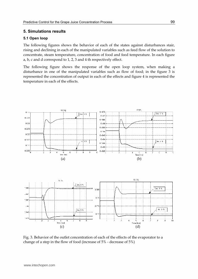
Fig. 8. Behavior of the temperature in the evaporator to a step change in feed concentration (increase of 5% - decrease of 5%).

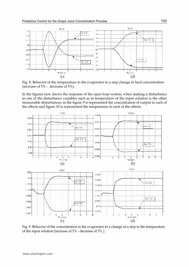
In the figures now shows the response of the open loop system, when making a disturbance in one of the disturbance variables such as in temperature of the input solution is the other measurable disturbances; in the figure 9 is represented the concentration of output in each of the effects and figure 10 is represented the temperature in each of the effects.

(a) (b)

(c) (d)

Fig. 9. Behavior of the concentration in the evaporator to a change of a step in the temperature of the input solution (increase of 5% - decrease of 5% ).

www.intechopen.com


(a) (b)

(c) (d)

Fig. 10. Behavior of the temperature in the evaporator to a change of a step in the temperature of the input solution (increase of 5% - decrease of 5%).

5.2 Close loop

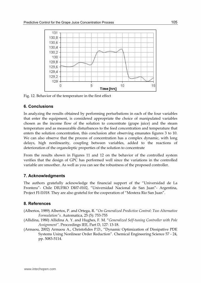
The following figures show the response of GPC controller, when conducted disturbances on the manipulated variables, ie giving an overview of the steam temperature and feed flow, one step at time 5 hours on the steam temperature and an increase to 10 hours in the feed stream.

Fig. 11. Behavior of the final product concentration at the outlet of the fourth effect

www.intechopen.com


Fig. 12. Behavior of the temperature in the first effect

6. Conclusions

In analyzing the results obtained by performing perturbations in each of the four variables that enter the equipment, is considered appropriate the choice of manipulated variables chosen as the income flow of the solution to concentrate (grape juice) and the steam temperature and as measurable disturbances to the feed concentration and temperature that enters the solution concentration, this conclusion after observing emanates figures 3 to 10. We can also observe that the process of concentration has a complex dynamic, with long delays, high nonlinearity, coupling between variables, added to the reactions of deterioration of the organoleptic properties of the solution to concentrate

From the results shown in Figures 11 and 12 on the behavior of the controlled system verifies that the design of GPC has performed well since the variations in the controlled variable are smoother. As well as you can see the robustness of the proposed controller.

7. Acknowledgments

The authors gratefully acknowledge the financial support of the “Universidad de La Frontera”- Chile DIUFRO DI07-0102, “Universidad Nacional de San Juan”- Argentina, Project FI-I1018. They are also grateful for the cooperation of “Mostera Rio San Juan”.

8. References

(Albertos, 1989) Albertos, P. and Ortega, R. “On Generalized Predictive Control: Two Alternative Formulation”s. Automatica, 25 (5): 753-755

(Allidina, 1980) Allidina A. Y. and Hughes, F. M. “Generalized Self-tuning Controller with Pole Assignment”. Proccedings IEE, Part D, 127: 13-18.

(Armaou, 2002) Armaou A., Christofides P.D., “Dynamic Optimization of Dissipative PDE Systems Using Nonlinear Order Reduction”. Chemical Engineering Science 57 - 24, pp. 5083-5114.

www.intechopen.com


(Aros, 2008), Nelson Aros, Carlos Muñoz, Javier Mardones, Ernesto Villarroel, Ludwig Von Dossow, “Sintonía de controladores PID basado en la respuesta de un GPC”II Congreso Internacional de Ingeniería Electrónica, ciudad de Madero – México, marzo de 2008.

(Asghari, 2006) Asghari, F. S.; Yoshida, H. “Acid-catalyzed production of 5-hydroxymethyl furfural from D-fructose in subcritical water”. Ind. Eng. Chem. Res. 2006, 45, 2163–2173.

(Barbieri, 1980) Barbieri, R., & Rossi, N. “Propietà fisiche dei mosti d’uva concentrati”. Rivista de Viticol. e di Enologia. Conegliano, No 1, 10–18.

(Bitmead, 1990) Bitmead, R.R.,M.Geversand V.Wertz “Adaptive Optimal Control: the Thinking Man‘s GPC”. Prentice-Hall.

(Camacho, 2004) Camacho, E.F. and Bordons, C. “Model Predictive Control”, Springer, London Limited.

(Clarke, 1987) Clarke, D.W. and Mohtadi, P.S. Tuffs, C. “ Generalized predictive control – Part I: thebasic algorithm”, Automatica 23 (2) 137–148.

(Christofides, 1998) Christofides P.D, “Robust Control of Parabolic PDE Systems”, Chemical Engineering Science, 53, 16, 2949-2965.

(Di Leo, 1988) Di Leo, F. “Caratteristiche fisico-chimiche dei mosti concentrati rettificati. Valutazione gleucometrica”. Vignevini, 15(1/2), 43–45.

(Ginz, 2000) Ginz, M.; Balzer, H. H.; Bradbury, A. G. W.; Maier, H. G. “Formation of aliphatic acids by carbohydrate degradation during roasting of coffee”. Eur. Food Res. Technol. 211, 404–410.

(Gogus, 1998) Gogus, F.; Bozkurt, H.; Eren, S. “Kinetics of Maillard reaction between the major sugars and amino acids of boiled grape juice”. Lebensm.-Wiss. Technol 31, 196–200.

(Ibarz, 1993) Ibarz, A., & Ortiz, J. “Reología de Zumos de Melocotón”. Alimentación, Equipos y Tecnología. Octubre, 81–86, Instituto Nacional de Vitivinicultura. Síntesis básica de estadística vitivinícola argentina, Mendoza. Varios números.

(Kam, 1999) Kam K.M., Tade M.O., “Case studies on the modelling and control of evaporation systems”. XIX Interamerican Congress of Chemical Engineering COBEQ.

(Kam, 2000) Kam K.M., Tade M.O., “Simulated Nonlinear Control Studies of Five Effect Evaporator Models”. Computers and Chemical Engineering, Vol. 23, pp. 1795 - 1810.

(Doyle, 1979) Doyle J.C., Stein G., “Robustness with observers”. IEEE Trans. on Auto. Control, Vol. AC-24, April.

(El-Farra, 2003) El-Farra N.H., Armaou A., Christofides P.D., “Analysis and Control of Parabolic PDE Systems with Input Constraints”. Automatica 39 – 4, pp. 715-725.

(Freudenberg, 1988) Freudenberg J., Looze D., Frequency Domain Properties of Scalar and Multivariable Feedback Systems. Springer Verlag, Berlín.

(Friedland, 1989) Friedland B., “On the properties of reduced-orden Kalman filters”. IEEE Trans. on Auto. Control, Vol. AC-34, March.

(Hoo,2001) Hoo, K.A. and D. Zheng, “Low-Order Control Relevant Model for a Class of Distributed Parameter Systems”, Chemical Engineering Science, 56, 23, 6683-6710.

(Kaya, 2002) Kaya A., Belibagh K.B., “Rheology of solid Gaziantep Pekmez”. Journal of Food Engineering, Vol. 54, pp. 221-226.

(Lelic, 1987) Lelic, M. A. and Wellstead, P. E, “Generalized Pole Placement Self Tuning Controller”. Part 1”. Basic Algorithm. International J. of Control, 46 (2): 547-568.

www.intechopen.com


(Lelic, 1987) Lelic, M. A. and Zarrop, M. B. “Generalized Pole Placement Self Tuning Controller. Part 2”. Basic Algorithm Application to Robot Manipulator Control. International J. of Control, 46 (2): 569-601, 1987.

(Middleton, 1990) Middleton R.H., Goodwin G.C., Digital Control and Estimation. A Unified Approach. Prentice Hall, Englewood Cliffs, N.J.

(Moressi, 1984). Moressi, M., & Spinosi, M. “Engineering factors in the production of concentrated fruit juices, II, fluid physical properties of grapes”. Journal of Food Technology, 5(19), 519–533.

(Ortiz, 2006) Ortiz, O.A., Suárez, G.I. & Mengual, C.A. “Evaluation of a neural model predictive control for the grape juice concentration process”. XXII Congreso 2006.

(Pandolfi, 1991) Pandolfi, C., Romano, E. & Cerdán, A. Composición de los mostos concentrados producidos en Mendoza y San Juan, Argentina. Ed. Agro Latino. Viticultura/Enología profesional 13, 65–74.

(Perry, 1997) Perry R., Perry’s Chemical Engineers Handbook. 7TH Edition McGraw Hill. (Pilati, 1998) Pilati, M. A., Rubio, L. A., Muñoz, E., Carullo, C. A., Chernikoff, R.E. & Longhi,

M. F. “Evaporadores tubulares de circulación forzada: consumo de potencia en distintas configuraciones. III Jornadas de Investigación´ n. FCAI–UNCuyo. Libro de Resúmenes, 40.

(Piva, 2008) Piva, A.; Di Mattia, C.; Neri, L.; Dimitri, G.; Chiarini, M.; Sacchetti, G. Heat-induced chemical, physical and functional changes during grape must cooking. Food Chem. 2008, 106 (3), 1057–1065.

(Rao, 1984) Rao, M. A., Cooley, H. J., & Vitali, A. A. “Flow properties of concentrated juices at low temperatures. Food Technology, 3(38), 113–119.

(Rubio, 1998) Rubio, L. A., Muñoz, E., Carullo, C. A., Chernikoff, R. E., Pilati, M. A. & Longhi, M. F. “Evaporadores tubulares de circulación forzada: capacidad de calor intercambiada en distintas configuraciones”. III Jornadas de Investigación. FCAI–UNCuyo. Libro de Resúmenes, 40.

(Sáenz 1986) Sáenz, C., & Costell, E. “Comportamiento Reológico de Productos de Limón, Influencia de la Temperatura y de la Concentración”. Revista de Agroquímica y Tecnología de Alimentos, 4(26), 581–588.

(Saravacos, 1970) Saravacos, G. D. “Effect of temperature on viscosity of fruit juices and purees”. Journal of Food Science, (35), 122–125.

(Schwartz, 1986) Schwartz, M., & Costell, E. “Influencia de la Temperatura en el Comportamiento Reológico del Azúcar de Uva (cv, Thompson Seedless)”. Revista de Agroquímica y Tecnología de Alimentos, 3(26), 365–372.

(Stefanov, 2003) Stefanov Z.I., Hoo K.A., “A Distributed-Parameter Model of Black Liquor Falling Film Evaporators”. Part I. Modeling of Single Plate. Industrial Engineering Chemical Research 42, 1925-1937.

(Suarez, 2010) Suarez G.I., Ortiz O.A., Aballay P.M., Aros N.H., “Adaptive neural model predictive control for the grape juice concentration process”. International Conference on Industrial Technology, IEEE-ICIT 2010, Chile.

(Zang, 1990) Zang Z., Freudenberg J.S., “Loop transfer recovery for nonminimum phase plants”. IEEE Trans. Automatic Control, Vol. 35, pp. 547-553.

(Zheng, 2002) Zheng D., Hoo K. A., “Low-Order Model Identification for Implementable Control Solutions of Distributed Parameter Systems”. Computers and Chemical Engineering 26 7-8, pp. 1049-1076.

www.intechopen.com


(Zuritz, 2005) Zuritz C.A., Muñoz E., Mathey H.H., Pérez E.H., Gascón A., Rubio L.A., Carullo C.A., Chemikoff R.E., Cabeza M.S., “Density, viscosity and soluble solid concentration and temperatures”. Journal of Food Engineering, Vol. 71, pp. 143 - 149.

www.intechopen.com

Frontiers of Model Predictive ControlEdited by Prof. Tao Zheng

ISBN 978-953-51-0119-2Hard cover, 156 pagesPublisher InTechPublished online 24, February, 2012Published in print edition February, 2012

InTech EuropeUniversity Campus STeP Ri Slavka Krautzeka 83/A 51000 Rijeka, Croatia Phone: +385 (51) 770 447 Fax: +385 (51) 686 166www.intechopen.com

InTech ChinaUnit 405, Office Block, Hotel Equatorial Shanghai No.65, Yan An Road (West), Shanghai, 200040, China

Phone: +86-21-62489820 Fax: +86-21-62489821

Model Predictive Control (MPC) usually refers to a class of control algorithms in which a dynamic processmodel is used to predict and optimize process performance, but it is can also be seen as a term denoting anatural control strategy that matches the human thought form most closely. Half a century after its birth, it hasbeen widely accepted in many engineering fields and has brought much benefit to us. The purpose of the bookis to show the recent advancements of MPC to the readers, both in theory and in engineering. The idea was tooffer guidance to researchers and engineers who are interested in the frontiers of MPC. The examplesprovided in the first part of this exciting collection will help you comprehend some typical boundaries intheoretical research of MPC. In the second part of the book, some excellent applications of MPC in modernengineering field are presented. With the rapid development of modeling and computational technology, webelieve that MPC will remain as energetic in the future.

How to referenceIn order to correctly reference this scholarly work, feel free to copy and paste the following:

Graciela Suarez Segali and Nelson Aros Oñate (2012). Predictive Control for the Grape Juice ConcentrationProcess, Frontiers of Model Predictive Control, Prof. Tao Zheng (Ed.), ISBN: 978-953-51-0119-2, InTech,Available from: http://www.intechopen.com/books/frontiers-of-model-predictive-control/model-predictive-control-for-concentration-process-

Documents

Predictive Control for the Grape Juice Concentration Processcdn.intechweb.org/pdfs/29695.pdf · · 2012-07-0390 Frontiers of Model Predictive Control The type and magnitude of degradation