Tallinn 2017

TALLINN UNIVERSITY OF TECHNOLOGY Faculty of Information Technology Department of Computer Systems

IAY70LT Mari Maisuradze

156394IASM

PREDICTIVE ALAYSIS ON THE EXAMPLE OF EMPLOYEE TURNOVER

Master’s thesis

Supervisor: Vladimir Viies PhD

Supervisor: Hannes Kinks MSc

Co-supervisor: Mari Pommer Swedbank

Tallinn 2017

TALLINNA TEHNIKAÜLIKOOL Infotehnoloogia teaduskond Arvutisüsteemide instituut

IAY70LT

Mari Maisuradze 156394IASM

ENNUSTAV ANALÜÜS TÖÖJÕU VOOLAVUSE NÄITEL

Magistritöö

Juhendaja: Vladimir Viies PhD

Juhendaja: Hannes Kinks MSc

Kaasjuhendaja: Mari Pommer Swedbank

3

Author’s declaration of originality

I hereby certify that I am the sole author of this thesis. All the used materials, references

to the literature and the work of others have been referred to. This thesis has not been

presented for examination anywhere else.

Author: Mari Maisuradze

09.06.2017

4

Abstract

The aim of the thesis is to try out how Predictive Analytics will perform for Human

Resource data, on the example of employee turnover measure. IBM example dataset and

Swedbank employee data, has been used for research. For implementing predictive

model Machine Learning algorithms have been used and their performances have been

evaluated.

The thesis is composed of four chapters:

Chapter One describes Predictive Analysis, its uses and the process flow of

implementation.

In chapter two different tools and algorithms used for implementing predictive

analysis is discussed. It is explained why python was selected tool for this thesis.

Also selected Machine Learning algorithms are described.

Chapter three describes HR tasks and responsibilities. Also importance of

employee turnover for organization and Predictive analytics role for HR is

explained. In addition, it includes information about Swedbank.

In chapter four is shown data preparation process on example of IBM data and

application of Machine Learning algorithms for Swedbank data.

As a result, out of the tested Machine Learning algorithms, Random Forest performed

the best with up to 98.62% accuracy. For tuning the parameters, grid search method

yielded better results compared to manual selection. In addition, decision trees were

interpreted as graphs for better understanding. Furthermore, features influencing

decision has been identified. For IBM dataset such features were related to monthly

income and age of employee.

This thesis is written in English and is 76 pages long, including 4 chapters, 31 figures

and 13 tables.

5

Annotatsioon ENNUSTAV ANALÜÜS TÖÖJÕU VOOLAVUSE NÄITEL

Viimase kahe aastakümne jooksul on arvutusvõimsuse kasv, andmesäilitusseadmete

mahtude suurenemine ja andmete digitaliseerimine toonud hüppelise kasvu infohulgas.

Suurte andmehulkadega on tekkinud aga ka uued probleemid, kuna infomüra on samuti

kasvanud ja andmetest olulise tähenduse leidmine on osutunud keeruliseks klassikaliste

andmetöötlus meetoditega. Teisest küljest on võimaldanud suured andmemahud masin-

ja süvaõppe algoritmide potensiaalil avalduda ning muuta ennustava analüüsi

praktiliselt tulemuslikumaks. Seetõttu võib täheldada järellainet, kus on tekkinud

massiline huvi uute andmetöötlus meetodite vastu ning soov olemasolevaid andmeid

efektiivsemalt analüüsida.

Magistriöö autor töötab töö kirjutamise hetkel Swedbanki inimressurside osakonnas,

kus kehtib sarnane olukord - omatakse suurtes kogustes andmeid töötajate kohta, kuid

nende kasutus piirneb raporteerimise ja kirjeldava andmeanalüüsiga. Seetõttu tekkis

autoril personaalne huvi suurendada andmete kasutuspotensiaali ennustava

andmeanalüüsi näol, võimaldamaks saada paremat arusaama tööjõu voolavusest ja selle

põhjustest Swedbankis. Kuna sage tööjõu vahetumine tähendab firma jaoks suuremaid

kulusid ja produktiivsuse langust talentide lahkumise tõttu, siis on oluline olla teadlik

tööjõu liikumise võimalikest stenaariumitest, mis aitab edaspidi paremini planeerida.

Käesoleva töö eesmärk on rakendada ennustavat analüüsi Swedbanki tööjõu voolavuse

näitel, leides töötajate lahkumise tõenäosusliku hinnangu ning selle eeldatavad

põhjused. Eesmärgi täitmiseks kõigepealt kirjeldatakse analüüsi teostamiseks vajalik

protsess ja selle etapid. Teiseks tuuakse välja masinõppe meetodid ja olemasolevad

tööriistad analüüsi teostamiseks ning võrreldakse nende sobilikkust antud töö eesmärgi

täitmiseks. Kolmandaks seletatakse lahti inimressursside osakonna töövaldkond ning

sellest tulenevad väljakutsed ja nõuded ennustava analüüsi rakendamisel. Viimaks on

teostatud andmete eeltöötlus ning seejärel viiakse läbi eksperimendid erinevate

masinõppe algoritmide ja parameetritega, leidmaks mudel, mis töötaks antud probleemi

6

jaoks kõige paremini. Eksperimente viidi läbi nii Swedbanki andmete kui ka näidis

avaandmete põhjal.

Töö tulemusena leiti, et otsustuspuudel põhinev Random Forest algoritm töötas kõige

paremini nii näidisandmete kui ka reaalsete andmete põhjal, andes ristvalideerimisel

tulemuseks kuni 98.62%. Näidisandmete analüüsi põhjal saab öelda, et suurimad

mõjurid töötaja lahkumisel on sissetulek, vanus ja töötatud aastad. Sama analüüs on

teostatud ka Swedbanki enda andmete põhjal.

Lõputöö on kirjutatud eesti keeles ning sisaldab teksti 76 leheküljel, 4 peatükki, 31

joonist, 13 tabelit.

7

List of abbreviations and terms

HR Human Resources

SVM Support Vector Machine

PCA Principal Component Analysis

HRIS HR Information Systems

HRM Human Resource Management

SWP Strategic Workforce Planning

PETA Predictive Analysis of Employee Turnover

KPI Key Performance Indicator

AUC Area Under the Curve

ROC Receiver Operating Characteristic

ANN Artificial Neural Network

MLP Multi-Layer Perceptron

KNN K-Nearest Neighbour

LDA Linear Discriminant Analysis

RBF Radial Basis Function

RF Random Forest

SAS Statistical Analysis System

NN Neural Network

BI Business Intelligence

8

Table of contents

Introduction ................................................................................................................ 12

1 Predictive Analysis .................................................................................................. 14

1.1 Modelling process ............................................................................................. 17

1.1.1 Defining outcomes ...................................................................................... 18

1.1.2 Understand the data, define the dataset ....................................................... 19

1.2 Data Preparation ................................................................................................ 21

1.2.1 Different data types .................................................................................... 21

1.2.2 Statistical techniques for cleaning and preparing data ................................. 23

1.3 Developing predictive model ............................................................................. 27

1.3.1 Learning methods ....................................................................................... 28

1.3.2 Different model categories .......................................................................... 28

1.4 Model evaluation ............................................................................................... 29

2 Methods and tools for Predictive Analysis ................................................................ 31

2.1 Machine Learning algorithms ............................................................................ 31

2.1.1 Random Forest algorithm ........................................................................... 34

2.1.2 Multi-Layer Perceptron............................................................................... 34

2.1.3 Support Vector Machine (SVM) ................................................................. 36

2.2 Tools for Predictive Analysis............................................................................. 37

2.2.1 Software trends ........................................................................................... 38

2.2.2 R ................................................................................................................ 41

2.2.3 SAS ............................................................................................................ 41

2.2.4 Python ........................................................................................................ 41

2.2.5 Matlab ........................................................................................................ 42

2.3 Tool selection .................................................................................................... 43

3 Predictive Analytics for human resources ................................................................. 44

3.1 Talent Analytics ................................................................................................ 44

3.2 Strategic workforce planning ............................................................................. 45

3.3 Employee Turnover ........................................................................................... 46

9

3.4 Predictive Analysis role in Talent Analytics maturity level ................................ 48

3.5 HR Analysis in Swedbank ................................................................................. 49

4 Building predictive model ........................................................................................ 51

4.1 Data preparation on example dataset.................................................................. 51

4.2 Modelling on Swedbank example ...................................................................... 57

4.2.1 ROC_AUC ................................................................................................. 57

4.2.2 Tuning parameters of Random Forest Classifier.......................................... 59

4.2.3 Tuning parameters for Multi-Layer Perceptron ........................................... 61

4.2.4 Tuning SVM............................................................................................... 62

4.3 Results and model Selection .............................................................................. 62

5 Summary ................................................................................................................. 65

References .................................................................................................................. 66

Appendix 1 – Additional Figures ................................................................................ 70

Appendix 2 – Python Code ......................................................................................... 73

10

List of figures

Figure 1 Interest over time of Big Data, Machine Learning and Data Science.............. 12

Figure 2 Applications of predictive analyses ............................................................... 15

Figure 3 The progression of analytics .......................................................................... 16

Figure 4 Predictive Analytics process flow ................................................................. 18

Figure 5 Variable types [11] ....................................................................................... 23

Figure 6 Graphical representation of an outlier [15] .................................................... 24

Figure 7 Distributions with a negative skew, no skew and a positive skew [16] ........... 25

Figure 8 Machine Learning algorithms [23] ................................................................ 32

Figure 9 Structure of Multi-Layer Perceptron [33]. ..................................................... 36

Figure 10 Classification using SVM on 2-dimensional space ...................................... 37

Figure 11 Popular tools among Data Scientists compared to Predictive Analytics [38] 39

Figure 12 Number of scholarity articles found in 2015, by r4stats [39] ........................ 40

Figure 13 Evolution of workforce planning methodology [55] .................................... 45

Figure 14 Analytical model of employee churn [55] .................................................... 47

Figure 15 Talent Analytics maturity model [61] .......................................................... 49

Figure 16 Unique values for features. .......................................................................... 53

Figure 17 Distribution of monthly income ................................................................... 54

Figure 18 Outlier values (in blue) of monthly income.................................................. 54

Figure 19 Distribution of MonthlyIncome ................................................................... 55

Figure 20 Distribution of MonthlyIncome after logarithmic transformation ................. 56

Figure 21 Receiver operating characteristic example [75]........................................... 58

Figure 22 max_features parameter for randomforestclassifier ..................................... 59

Figure 23 Branch of decision tree. ............................................................................... 63

Figure 24 Feature importance ...................................................................................... 64

Figure 25 n_estimators parameter for randomforestclassifier ...................................... 70

Figure 26 min_sample_leaf parameter for randomforestclassifier ............................... 70

Figure 27 Replaced outliers ......................................................................................... 71

Figure 28 alpha (1/Value of parameter) parameter for MLPClassifier ......................... 71

Figure 29 max_iter parameter tuning for MLPClassifier .............................................. 72

Figure 30 hidden_layer_sizes parameter tuning for MLPClassifier .............................. 72

Figure 31 hidden_layer_sizes parameter tuning .......................................................... 72

11

List of tables

Table 1 17th annual KDnuggest Data Science Software poll [14] ................................ 38

Table 2 Data Categorisation. ....................................................................................... 52

Table 3 Variable categorisation. .................................................................................. 52

Table 4 Continuous variables ...................................................................................... 55

Table 5 Skewness of continuous variables ................................................................... 55

Table 6 Confusion Matrix ........................................................................................... 57

Table 7 Selected parameters for Randomforestclassifier .............................................. 60

Table 8 Performance results of differently tuned Randomforestclassifier ..................... 60

Table 9 MLPClassifier test results. .............................................................................. 61

Table 10 MLPClassifier performance using tuned parameters ..................................... 61

Table 11 MLP tuned parameters.................................................................................. 62

Table 12 SVM parameters ........................................................................................... 62

Table 13 Model selection ............................................................................................ 63

12

Introduction

Background and motivation

With the development of modern information systems and databases that are capable of

holding immense amounts of data, the need for analysing it has become progressively

more relevant. This can be seen in trends of Google search, using keywords ‘Big data’,

‘Data Science’ and ‘Machine Learning’ (Figure 1). Also the fact that universities have

started offering certification courses and master’s degrees in Predictive Analytics and

Big Data Analytics reflects the growth and popularity of this field.

Figure 1 Interest over time of Big Data, Machine Learning and Data Science

The raw data itself does not carry much value without any further processing and

analysing. On Figure 1it is clearly visible that as Big Data became relevant problem for

modern world, interest in Data Science and Machine Learning grew. There are different

types of Data Analytics starting from Descriptive Analytics evolving to something more

advanced, like Predictive Analytics.

Predictive analysis allows the analyst to operate on historical and current information as

well as predicting the likely future environment. This predictive insight promotes much

better decision making and improved results.

2010 2011 2012 2013 2014 2015 2016 2017

Big data

Machine Learning

Data Science

13

Use of predictive analytics is wide, it enables companies to improve almost every aspect

of their business.

As Human Resources (HR) possesses a massive amount of employee data, demand for

analyses if high. However, HR Information Systems (HRIS) are often underfunded

compared to information systems of other domains of enterprise, which are directly

connected with main business [1]. This leads to the fact that HR data contains lot of

noise and errors. Therefore, building accurate analytical model is challenging for HR.

One of the uses of Predictive Analytics for Human Resources (HR) is predicting

employee turnover, attrition or retention. Employee turnover has number of negative

impacts including loss of enterprise knowledge, costs associated with leaving and

replacement. To accurately determine who is leaving and what is the underlying reason

are key issues for HR workforce planning.

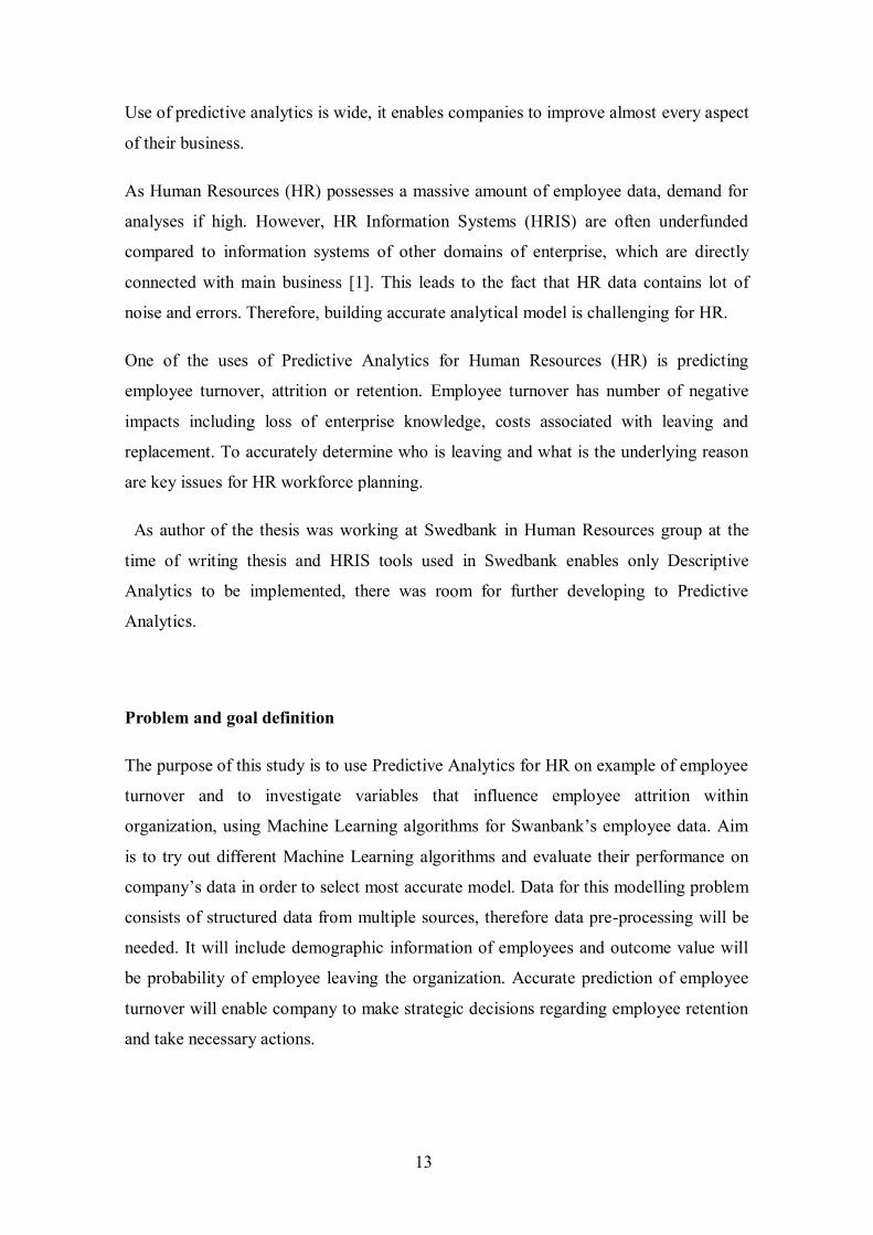
As author of the thesis was working at Swedbank in Human Resources group at the

time of writing thesis and HRIS tools used in Swedbank enables only Descriptive

Analytics to be implemented, there was room for further developing to Predictive

Analytics.

Problem and goal definition

The purpose of this study is to use Predictive Analytics for HR on example of employee

turnover and to investigate variables that influence employee attrition within

organization, using Machine Learning algorithms for Swanbank’s employee data. Aim

is to try out different Machine Learning algorithms and evaluate their performance on

company’s data in order to select most accurate model. Data for this modelling problem

consists of structured data from multiple sources, therefore data pre-processing will be

needed. It will include demographic information of employees and outcome value will

be probability of employee leaving the organization. Accurate prediction of employee

turnover will enable company to make strategic decisions regarding employee retention

and take necessary actions.

14

1 Predictive Analysis

Over the last two decades with the advancements of computer processing and data

storage capabilities the volumes and complexity of data stored by companies throughout

the world have increased rapidly. The global growth of this information has brought

along a need for better methods to process and analyse these large datasets, also known

as Big Data. Interest in Data Analytics and Machine Learning methods has now become

increasingly popular as an after wave of the data growth.

Terms such as “Data Science”, “Data Analytics”, “Predictive Analytics”, “Predictive

Modelling”, “Data Mining” and “Machine learning” are still new, often used

ambiguously and interchangeably.

Term Data Science refers everything that is related to data cleansing, preparation and

analysis in order to extract insights and understandable information from data [2]. It

combines mathematical, statistical methodologies alongside with programing. Data

Analytics on other hand focuses more on deriving conclusions based on raw data. A

huge amount of data that cannot be stored or processed within given timeframe using

standard technologies is called Big Data.

Data Mining is a process of data collection, warehousing and analysing [3]. Before Big

Data existed businesses were using basic analytics (essentially numbers in a spread

sheet that were manually examined) to uncover insights and trends [4]. Descriptive

statistical analysis is used to quantitatively summarize data in a manner that would

describe basic features. Due to the progressive use of technology, Machine Learning

algorithms became more popular over descriptive statistical methodologies. Machine

Learning algorithms are capable of learning on examples of data. They identify hidden

patterns in enormous volumes of raw data and can adjust and match new data

accordingly. This gave opportunity not only to describe and show features of data but to

predict future values.

Predictive Analytics incorporates techniques of statistics, Data Mining, Machine

Learning, predictive modelling and business knowledge (of how to interpret information

and use it to create value) [5]. By analysing historical and current data it exploits

patterns, identifies risks and opportunities and makes predictions about future.

15

Advanced analytics capabilities gave companies potential to get real time insights of

business processes, fuelled making better decisions, had direct impact on avenue and led

to increased profits. It is widely used across different range of companies, because of its

positive influence on business. Predictive Analytics can help companies to grow

revenue, reduce fraud by detecting suspicious activities in transactional data, improve

operations, track trends, increase sales, reduce churn, cross-sell campaigns and help to

better understand customer behaviour. It helps to target right customer groups, enabling

companies to make personalized offers. Predictive Analysis found its way in HR as

well, smarter management of human capital is relatively new. More and more

companies are turning to Predictive Analytics to drive better hiring decisions, by

targeting right applicants for right positions. Or by providing managers relevant reports

of identifying factors that leads to enhance productivity, establish proper carrier and

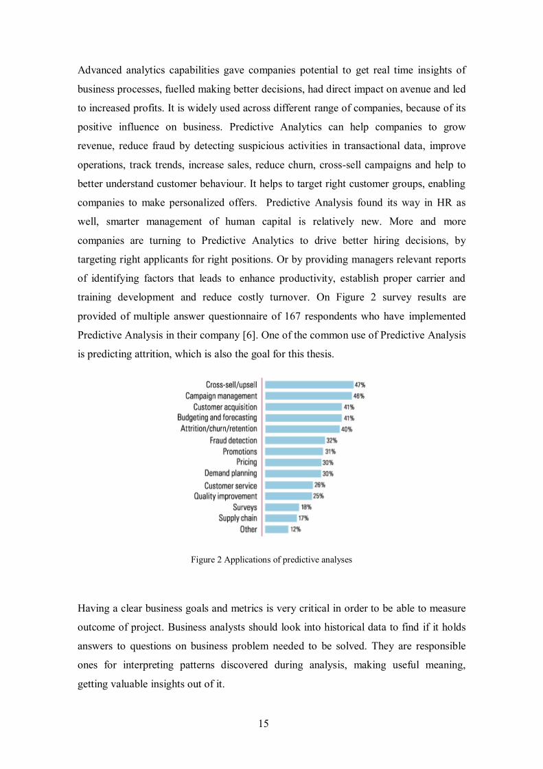
training development and reduce costly turnover. On Figure 2 survey results are

provided of multiple answer questionnaire of 167 respondents who have implemented

Predictive Analysis in their company [6]. One of the common use of Predictive Analysis

is predicting attrition, which is also the goal for this thesis.

Figure 2 Applications of predictive analyses

Having a clear business goals and metrics is very critical in order to be able to measure

outcome of project. Business analysts should look into historical data to find if it holds

answers to questions on business problem needed to be solved. They are responsible

ones for interpreting patterns discovered during analysis, making useful meaning,

getting valuable insights out of it.

16

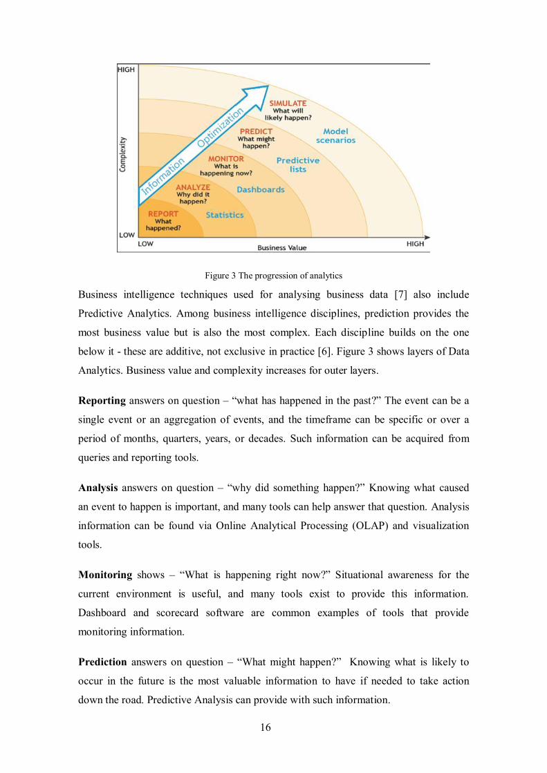
Figure 3 The progression of analytics

Business intelligence techniques used for analysing business data [7] also include

Predictive Analytics. Among business intelligence disciplines, prediction provides the

most business value but is also the most complex. Each discipline builds on the one

below it - these are additive, not exclusive in practice [6]. Figure 3 shows layers of Data

Analytics. Business value and complexity increases for outer layers.

Reporting answers on question – “what has happened in the past?” The event can be a

single event or an aggregation of events, and the timeframe can be specific or over a

period of months, quarters, years, or decades. Such information can be acquired from

queries and reporting tools.

Analysis answers on question – “why did something happen?” Knowing what caused

an event to happen is important, and many tools can help answer that question. Analysis

information can be found via Online Analytical Processing (OLAP) and visualization

tools.

Monitoring shows – “What is happening right now?” Situational awareness for the

current environment is useful, and many tools exist to provide this information.

Dashboard and scorecard software are common examples of tools that provide

monitoring information.

Prediction answers on question – “What might happen?” Knowing what is likely to

occur in the future is the most valuable information to have if needed to take action

down the road. Predictive Analysis can provide with such information.

17

Predictive Analytics is followed by Prescriptive Analytics questioning “how can we

make it happen?”

While Predictive Analysis is about understanding most likely future scenario,

Prescriptive Analytics suggest decision options.

1.1 Modelling process

Building a Predictive Analytics solution is a continuous and an iterative process which

requires an integrated enterprise wide approach [8]. Since business objectives and

related datasets vary company to company Predictive Analysis process might be

somewhat different, but it can be structured as six steps approach shown on Figure 4.

1. Identify the business objective - Defining outcomes and business objectives is very

first step for building a Predictive Analytics project.

2. Prepare the data - Data collection and data analysis are required for preparing data,

to be later used in predictive modelling. Data should be cleaned and transformed, so

that useful information can be concluded. Statistical analysis can be applied to

validate assumptions, by testing using standard statistical models. Data Mining can

be used for data preparation from multiple sources.

3. Develop the Predictive model - Predictive modelling provides ability to

automatically create accurate predictive models about future. Predictive modelling

is process of creating, testing and validating a model to best predict the probability

of outcome. Modelling methods are for example: Machine Learning, AI, statistics.

4. Test the model

5. Deploy the model - Predictive model deployment provides the option to deploy the

analytical results into the everyday decision making process to get results, reports

and output by automating the decisions based on the modelling.

6. Monitor for effectiveness - Models are managed and monitored to review the model

performance to ensure that it is providing results expected

18

Figure 4 Predictive Analytics process flow

To start with Predictive Analytics project Data Science team and technological

resources are needed, as well as business knowledge. First, a clear business objective

should be set, what is expected to achieve and what should be outcome. Business

stakeholders should be familiar with the domain. They should identify which features of

data are relevant and important for model, there might be a need to create new variables

or derived features in order to improve model. Data scientist will deploy model.

Afterwards business should evaluate outcome. Business analysts should analyse

identified data patterns and make useful and meaningful value out of it.

1.1.1 Defining outcomes

Defining outcome of the project is the preliminary step in building the predictive model.

By identifying what problem to solve, what is the goal and what should be the output of

project, success measures will be defined. Having clear business objectives are critical.

Output of the project in Machine Learning context is a target variable. Defining target

variable in dataset is rather a simple and straightforward process.

19

1.1.2 Understand the data, define the dataset

In order to enhance project results preparing dataset plays a big role, before statistical

analysis, data-mining and Machine Learning algorithms can be applied. Data needs to

be obtained and prepared for model to work. Data points that are relevant for analysis

are important attributes. Available data should be assessed and need of any additional

data should be determined. Data from different sources should be put together.

After identifying business objectives, outcome metric and business process data sources,

fields that might have direct impact on outcome predictor variables should be chosen.

Analysts should understand business process and data source nuances that would assist

in collecting and shaping data for analysis process [9].

Companies gather knowledge about their customers, employees, at every opportunity.

Social media posts, purchase histories, geographical locations, bank statements - all this

information piles up into Big Data, out of which very little will be actually analysed. It

is important to filter out important variables, cut the noise and convert it into smart data.

Value should be found in the data. Selecting right data, cleaning, processing and

preparing it for analysis is time consuming process and requires a lot of patience.

Whichever company will analyse such data accurately and effectively will profit from

it.

Depending on project, data preparation might be a one-time activity or might need

periodic updates. Dataset should include few columns, several predicators, independent

variables (location, salary, age, period, etc.) and one outcome measure (e.g. attrition).

Preparation process involves choosing outcome measure for evaluation, identifying

potential influencer variables, creating features and generating datasets. Unobserved

relationships between variables that are not captured by input predictors are causing

noise in data. The more noise is there in the data, the more records it will need to

overcome it.

Within big companies raw data usually has multiple sources. It is being captured during

various business processes or it might come from third party. Usually the data is

distributed within different database servers or in worst cases, scattered across hard

drives of company’s computers. In any case there will be a need of data preparation,

20

including cleansing, spotting missing or duplicate values. Fields related in those

different systems should be joined together from multiple tables in order to create single

unified, flattened file. Relevant data should be separated from noise. Attributes with

better predictive possibilities should be selected and stable algorithm should be chosen

to run on data.

Data can be collected in different ways for predictive modelling. It can be purely based

on existing data, which is called data driven approach or can be selected by domain

experts, known as user driven. In case of data driven approach prior knowledge of

domain or data is not required. Data Mining methods can be applied without any

specific goal, but still enabling to acquire understanding to reveal hidden patterns and

generate new categorizations. Oppositely, user driven analytics requires in depth

knowledge and expertise of business domain. Subset of data is selected strategically, in

relevance to support ideas important for business. Since only parts of data are being

used for user driven approach to test the ideas, hidden patterns in data can be missed

and stay undiscovered.

Inconsistent data formats, "dirty data", redundant data and outliers can undermine

quality of analytical findings [9].

Depending on level of outcome granularity, input data should be aggregated. If data is

collected within different time periods and for outcome prediction time sequences and

dates are important predictors, they can be rolled up to durations. For example leaving

date and start date can be rolled up as years in company. Data should reflect what

actually is happening in the real world at right level of granularity. Overly aggregated

data or data revealing too many details will have effect on quality of results. For

example, if outcome metric is day based the data should be prepared at day level, not

aggregated on monthly level. Also events that happened closest to outcome are stronger

predictors than remote events that happened long time ago.

If needed data should be reduced in volume and in dimension. Only subset of data

should be chosen for analysis that will represent the data as a whole better, and

dimensionally only more important features should be selected. Such subset is called

nucleus or smart data. It is best to start with fewer columns and add more data later.

Another approach would be to start with all available features and filter them while

21

experimenting, leaving only most important attributes that gives higher accuracy for

prediction. Or running multiple models and choosing one that gives best results.

Usually second approach is chosen when problem is too complex. This enables data

scientists to experiment with variables that are not commonly associated with domain,

by running algorithms several times with different variables, including or excluding

certain ones. If too many variable fields are used, there is a high risk that data will be

over-fitting. Over-fitting captures noise in data. Predictive model will be memorising

unnecessary details and it will become overly complex and unreliable. But if model is

too simple then there will be risk of under-fitting, model won't be able to capture

underlying patterns in data.

1.2 Data Preparation

After determining data that needs to be modelled, data cleansing and shaping will be

needed. Data preparation process may include next steps: select outcome metric and

predicator variables, determine how much data to model, cleanse and prepare data.

Different data types and measurement level in dataset should be identified for each

variable. Afterwards data should be assessed for outliers, missing or incorrect values.

Skew and high cardinality in data should be removed [9].

1.2.1 Different data types

For different types of data, there are different approaches of analyses. Data used for

Predictive Analysis can exist in structured or unstructured form.

Data that has high level of organization and follows consistent order is a structured

data. Such data is easy to query and search. Structured data is usually stored in well-

organized systems like databases, excel, etc. Such systems make data management easy.

Unstructured data on the other hand is the data in its free form, non-tabular, unshaped

and dispersed. Such data is not easily retrievable and esquires deliberate intervention to

make sense of it. Examples of unstructured data would be web pages, e-mails,

documents, and files in different formats whether text, audio, and/or video in scattered

locations. Unstructured data is hard to categorize and to choose relevant attributes from

it. Also analysing unstructured data takes more time and effort. For computer systems it

22

is hard to impossible to analyse such free form data. Unfortunately there is more

unstructured data out there than structured.

There are streamed or static types of data [10].

Static data as the word suggests is the data that does not change, is enclosed, self-

contained or controlled. Static data might require cleansing and pre-processing before it

can be used for analysis.

Streaming data is a real-time data, is dynamic and changes continuously. Examples of

such data would be stock prices while market is open, weather forecast and so on.

In addition to categorizing data by types and forms, it can be differentiated by its

categories.

Data that is gathered via surveys and shows information about what participants think or

feel is called attitudinal data. Attitudinal data is analysed to understand insights of

motivation of behaviour. Such data cannot be always reliable, it depends on

participant’s honesty and how objective they were.

More reliable category of data is behavioural data, which represents what actually

happened. It is more like observational data of behaviour or triggers of behaviour.

Example of such data can be business customer interaction like sales transactions.

Information including age, race, location, education level, marital status and similar are

categorised as demographic data. Such data gives better insights and helps to target

relevant segment of demographics.

Data items are called variables, because they may change value. Age, gender, country

are examples of variables. Data objects are also referred as attributes or features.

In statistical analysis variables are categorised as qualitative or quantitative variables

[11]. Qualitative variables can be placed into different categories according to their

distinct qualities and characteristics. For example, gender, citizenship, location are

qualitative variables. Quantitative as word suggests, are numerical variables that can be

ranked or ordered. Quantitative variables can be continuous, they can have infinite

number of values or discrete, meaning that values are countable. Examples of discrete

23

variables would be number of employees, children and so on, while continues variables

are such as temperature, stock price and etc.

Figure 5 Variable types [11]

The type of analysis that is sensible for given dataset depends on the level of

measurement. There are four common types of measurement scales by which variables

are categorised, shown on Figure 5. When there is no distinctive order in variables and

they can be classified in to mutually exclusive categories, such variables are nominal of

type. For example, gender is nominal type of variable. It can only have mutually

exclusive values. But if variables can be ranked, rated or ordered in a meaningful way

they are called ordinal variables. Grades can be example of ordinal variables. If interval

between ordered variables is equal it is called interval type and if interval matters but in

addition there can be true zero or absence, it is called ratio. Temperature, calendar dates

are examples of interval type. Height, weight, time, salary are examples of ratio. There

can be absence of weight, zero pounds but 0 Celsius does not mean that there is absence

of temperature. Nominal and ordinal types are categorical (qualitative) variables. It is

not possible to calculate mean or average value for nominal variables. For ordinal data it

is possible to calculate mean or average but needs to be justified. Interval and ratio

variables are quantitative, so they can be discrete or continuous.

1.2.2 Statistical techniques for cleaning and preparing data

Data validity should be checked and corrected, as error in data can lead to inaccurate

predictions. Big Data usually consists of data in different forms like, unstructured text

data such as emails, tweets comments and so on. It may also include structured data like

bank transactions, demographic data, etc. Integration and aggregation of such data from

24

different sources is a complex task. Usually it is data scientist task to standardize and

uniform such data with data providers, which varies from company to company and

project to project.

Except of different forms of existing data Big Data challenges are its volume, mass of

data and velocity (rate at which data is increasing in volume). For databases with high

velocity, capturing smart data out of Big Data is more challenging. Usual approach is to

capture data as it can be afforded. Overall Big Data is a wide variety of large volume of

data, generated with high velocity [12].

For unstructured data semantic search may be applied, using ontology of domain (set

of similar terms and concepts of domain) [13]. There are number of softwares allowing

to tag semantically similar words together in same domain. Such semantic case search

is more accurate than key-word based search. Unstructured Information Management

(UIM) is an example of system that analyses large volumes of unstructured data [14].

Outliers are values that exceed three standard deviations from the mean [9]. On Figure

6 is shown how outlier value is separated from rest of the data values. Outlier influence

can be reduced by using transformations or converting the numeric variable to a

categorical using binning.

Figure 6 Graphical representation of an outlier [15]

Predictive algorithms assume the input information is correct. Incorrect values should

be treated same way as missing values if there are only a few. If there are a lot of

inaccurate values, data source repairments might be applied.

25

The most common repair for missing values is imputation. Deleting a row is bad

approach, because useful data might get lost. Better approach would be to replace

missing value, by inserting expected value for missing value, using a mean or median in

case of numerical variables. For categorical variables missing values can be replaced by

computed value from a distribution, for example most frequent value.

In case if in dataset continuous variables are used, spread of such data and its central

tendency should be checked. Various statistical metrics exist that can be used for

visualisation of data distribution. If continuous variables are not normally distributed,

skewness should be reduced for optimal prediction [9]. On Figure 7 is shown

visualisation of negative and positive skew.

Figure 7 Distributions with a negative skew, no skew and a positive skew [16]

For example to calculate skewness Pearson’s second coefficient of skewness equation

(1) or Moment coefficient of skewness (2) can be used.

Pearson’s second coefficient of skewness [17]:

𝑆𝑘𝑒𝑤𝑛𝑒𝑠𝑠 =3(𝑀𝑒𝑎𝑛−𝑀𝑒𝑎𝑑𝑖𝑎𝑛)

𝑆𝑡𝑎𝑛𝑑𝑎𝑟𝑑 𝐷𝑒𝑣𝑖𝑎𝑡𝑖𝑜𝑛 (1)

Moment coefficient of skewness [18]:

𝑔 =𝑚3

𝑚𝑚

32

(2)

Where 𝑚3 =∑(𝑥−�̅� )3

𝑛 and 𝑚2 =

∑(𝑥−�̅� )2

𝑛 , x̅ is the mean and n is the sample size.

26

Depending on the direction of skewness different transformations can be used to reduce

it. Most common method is logarithmic transformation for positive skew, for negative

skew square or cubic transformation can be used [19].

Datasets kept in corporate warehouses usually have high-cardinality fields for data

identification. High-cardinality fields are categorical attributes that contain a very large

number of distinct values. Examples include names, ZIP codes or account numbers.

Even though these variables can be highly informative, high-cardinality attributes are

rarely used in predictive modelling [20]. The main reason is that including these

attributes will vastly increase the dimensionality of the dataset, making it difficult or

even impossible for most algorithms to build accurate prediction models.

Ordinal variables are also problematic for predictive models. Ordinal data consists of

numerical scores on an arbitrary scale that is designed to show ranking in a set of data

points. For example, low, medium and high are ordinal, different states are ordered in a

meaningful way. Predictive algorithms will assume the variable is an interval or ratio

variable and may be misled or confused by the scale. Ordinal values should be therefore

transformed into numeric values. Other approach will be to create dummy variables for

categorical variables in general.

In dataset redundant data, duplicates or other highly correlated variables that carry the

same information should be removed. If one predictor variable can be linearly predicted

by other with a substantial degree of accuracy, they are highly correlated [21].

Collinearity can cause some regression coefficients to have wrong sign. It can be

examined by computing correlation coefficient for each independent variable.

To calculate correlation between X and Y variables next formula can be used:

𝑟 =𝑐𝑜𝑣(𝑋, 𝑌)

𝑠𝑥𝑠𝑦=

𝑛(∑𝑥𝑦) − (∑𝑥)(∑𝑦)

√[𝑛∑𝑥2 − (∑𝑥)2][𝑛∑𝑦2 − (∑𝑦)2] (3)

Where: 𝑟 is Pearson correlation coefficient, 𝑐𝑜𝑣(𝑋, 𝑌)is covariance, 𝑠𝑥 and 𝑠𝑦 are

standard deviations of sample sets 𝑋 and 𝑌 respectively (𝑥 ∈ 𝑋, 𝑦 ∈ 𝑌) and 𝑛 is number

of values in both dataset.

27

If variables are identical, but there is still need to retain difference between them, ratio

variables can be used instead or Principal Component Analysis (PCA) output can be

used as input variables. PCA is technique for reducing dimensionality, it transforms

large amount of features of dataset into “principal components” that summarizes the

variance within the data [22]. This “principal components” are calculated by finding

linear combination of features having maximum variance, there should be no correlation

within components.

To get more meaningful information from the data, feature engineering can be applied.

From data that already exists more useful features can be created, that will better

describe the process that is being predicted, improving pattern detection and enabling

more actionable insights to be found. For example, some variables can be combined,

showing information associated with interactions. More complex concepts can be

represented by ratios. Some features can be aggregated by computing the mean

(average), minimum, maximum, sum, or by multiplying two variables together and

ratios made by dividing one variable by another. Some variables can be transferred,

replaced by a function. Such transformations are usually used to change a scale of

variable, in order to standardize the value for better understanding.

After cleaning data, it may be needed to be split it into training and test sets. Such sets

can be separated by randomly selecting records. Usually training data set is bigger than

test, but it is best if both sets contain just enough rows to reflect real scenario. For

example, prediction will not be accurate if all of the same type of outcome is in test-

data, not leaving room for training or other way around. Sample data is chosen

randomly out of whole population. Sample data should be chosen so that, analysis on

whole population will have realistic accuracy.

1.3 Developing predictive model

Most algorithms used for predictive analyses have been out there for decades, but only

recently data scientists started to mine data effectively. Since, just recently data

gathering has become cheaper and faster.

Algorithm that should be used for data modelling should be determined and developed.

28

1.3.1 Learning methods

There are two main Machine Learning types: supervised and unsupervised [23].

In case of supervised learning, machine is told what the correct answers are, input

training data is labelled and results are known. Machine is corrected when wrong

prediction is made, so it learns on previous experience. Supervised learning method is

suitable for both classification and regression problems.

When data is not labelled and results are unknown unsupervised learning method is

used. Such algorithms are used for clustering and association problems.

There can be mixture of both labelled and unknown data as well. Such learning style is

called semi-supervised learning. For such learning methods, algorithm should organize

data and then predict.

In addition to those three there is also reinforcement learning, which uses reward

function for training. Essentially in reinforcement learning an agent will be rewarded as

it transitions to certain states or executes actions. The algorithm tries to optimize its

actions for maximizing the reward. For example, a Machine Learning algorithm can be

taught to play a computer game, if the agent has a control over the inputs and is

rewarded based on the game score, resulted from the correct sequence of inputs. [24]

1.3.2 Different model categories

Most Predictive Analytics tools include algorithms for modelling. Building a model

with best accuracy possible will take more time. Experiment with different approaches

should be held and outcomes should be re-evaluated. Model requires continuous updates

to keep relevance, building a predictive model should be an on-going process.

Predictive Analysis models can be categorised various ways. For example, they can be

categorised by different approaches like:

Predictive Analysis model analyses dataset to predict next outcome. Outcome can be

binary, numerical, yes/no value or have a combination of those.

29

Classification model works by identifying different groups within data and indicates

whether an item belongs to certain class. Predictive model can be built on top of

classification model.

Decision model uses strategic plans for complex case scenarios for identifying best

action.

Association models are identifying associations existing in data.

Often predictive models use mix of these approaches. Widely used technique for

predictive modelling is data classification. Classification models are often called

classifiers.

First using data clustering data is being organized into groups of similar objects (classes

which describes data). Large volumes of data are separated into clusters, in a group of

similar objects [25]. First data is converted into matrix, modelled as table where each

raw contains object and columns represent features. Data clustering is a way of

modelling data, where subset of data represents whole cluster. Based on learned

experience classification algorithm predicts the class of newly input object, to which

category it belongs. Data classification is used for labelling data objects in to similar

object clusters. Data classification is processed into two stages; during Learning stage

classification rules are applied on training set of data, to learn hidden relationships

within data. Afterwards, during Prediction stage it is evaluated on test data.

Depending on output type, different types of algorithms can be applied. If type of

outcome is qualitative, classification algorithms should be used. For quantitative,

regression type of algorithms should be used. Some algorithms can be applied for both

types of outputs.

1.4 Model evaluation

Because of the noise and stochastic characteristic of real world data, it is nearly

impossible to predict without an error [26]. Cross validation is common to be used for

model selection. For cross validation, dataset is randomly divided into two parts. First

part is used for training the model, while other is used to test the model. This type of

random split of dataset can be done multiple times with different choices of training and

30

test sets. Next outcome can be averaged, this helps to reduce the variance. K-fold cross

validation is using same principle. It divides dataset in K consecutive sets or folds and

then for each fold trains model on K-1 folds, leaving one fold for validation. After K

iteration performance measures are being averaged [27]. Ten-fold cross validation

iterates ten times and chooses best model. Ten times iteration is generally

recommended, because it is large enough for averaging and small enough to run fast.

To compare outcome of classification methods for given problem and dataset, they

should be evaluated using different criteria such as accuracy, speed, robustness,

scalability and interpretability. Algorithm should correctly classify and label data

objects (accuracy), it should not be computationally costly (speed), should overcome the

noise in data (robustness) and should be able to efficiently classify large amount of data

(scalability).

For indicated problem of this thesis, ten-fold cross validation will be used for measuring

accuracy of tuned models. First best parameters will be chosen for each model, by trial

error approach. Afterwards for indicating classification accuracy, misclassification rate

will be calculated by counting wrongly predicted values and percentage of errors out of

all predictions made on test dataset. Speed, robustness and scalability will not be

measured since data used for modelling is not large enough.

31

2 Methods and tools for Predictive Analysis

Due to the fact that there is a large number of different algorithms and tools available

for doing Predictive Analysis, they will be examined separately in this chapter in order

to help choosing the best methods to efficiently predict employee turnover. A set of

algorithms and tools gathered under an umbrella term ‘Machine Learning’ will be

concentrated on, as they have shown the most promise predicting on large datasets.

2.1 Machine Learning algorithms

Machine learning uses computer program that learns by analysing data. The more data

there is, the better the program can learn. We are teaching the program rules and

program itself is getting better at it by learning and practicing. Machine learning

algorithms are more suitable for complex data and work better with huge sets of training

examples [23].

There are many different types of Machine learning algorithms. On Figure 8 Machine

Learning algorithms are categorised according to methodologies they use for prediction.

32

Figure 8 Machine Learning algorithms [23]

Regression algorithm - Linear and logistic are most widely used type of regression

algorithms for Predictive Analysis. Regression analysis finds relationship between

target variables and predicators, then refines this relationship by measuring error

(Gradient descent), when sum of errors is least.

Instance-based algorithms - Instance-based Algorithms also might be found with the

name of winner-take-all methods and memory-based learning. New data is compared to

training datasets and using similarity measure best match is found. K-Nearest

Neighbour (KNN) is one of the popular algorithms of Instance-based learning methods.

33

Regularization algorithms - It is supervised learning algorithm. Based on the

complexity of model it gives disadvantage. Regularization algorithms are usually used

as extension of regression methods.

Decision Tree algorithms - By learning decision rules deduced from data features

decision trees predict the value of new data object. They use supervised learning style

and can be applied for both classification and regression problems.

Bayesian algorithms - Methods that are based on Bayes Theorem are Bayesian

Machine Learning algorithms. They can be used for bot classification and regression

problems. Naive Bayes algorithm is most popular Bayesian algorithm.

Clustering algorithms - Such algorithms are used for organizing data objects into

groups of similar objects. There are hierarchical and centroid based modelling

approaches. K means/median and hierarchical clustering algorithms are one of the

mostly used clustering algorithms.

Association Rule Learning algorithms - By observing relationships within data

variables association rule learning methods extract rules that are important to dataset.

Artificial Neural Network algorithms - “a computing system made up of a number

of simple, highly interconnected processing elements, which process information by

their dynamic state response to external inputs” [28]. ANNs consist with multiple nodes,

which imitate biological neurons of human brain.

Deep Learning Algorithms - Deep Learning Algorithms are updated version of ANN

that concentrates on building more complex and large NN.

Dimensionality Reduction algorithms - Dimensionality Reduction Algorithms uses

unsupervised learning style, to organize data groups. They can be used for classification

and regression algorithms. Principal Component Analysis (PCA) and Linear

Discriminant Analysis (LDA) are popular examples.

Ensemble algorithms - Ensemble Algorithms combine results of other smaller models

to make overall prediction. There are different technics of how to combine models

together and which type of models to choose. Bootstrapped Aggregation (Bagging) and

Random Forest are examples of such algorithms.

34

2.1.1 Random Forest algorithm

Random Forest is an ensemble type of Machine Learning algorithm, which means that it

consists of combination of several models to solve single prediction problem. Random

Forest ensembles a set of decision tree models. A decision tree is composed of a series

of decisions that can be used to classify an observation in a dataset [29]. For complex

problems one decision tree (one set of rules) is not enough for accurate classification.

Random Forest is based on bootstrap aggregation or also called bagging technique - it

uses combination of decision trees to increase accuracy. Bootstrap statistical method is

used for estimating quantity, for example mean from sample data. Bagging tries to

estimate the best mean value by taking a large number of samples from data, calculating

mean for each of the sample and calculating average of those mean values.

Random Forest algorithm from sample set selects a large number of random subsets and

on each subset creates decision tree. Each decision tree created this way uses a different

set of rules, therefore they are different classifiers. Decision trees tend to overfit,

meaning they have low bias and high variance. Contrariwise, since Random Forest

algorithm builds a large collection of de-correlated trees and then averages them, it

reduces variance [30].

Random Forest algorithm can be used for both classification and regression problems.

In case of regression problem, the output of the algorithm is mean. In case of

classification problem, the output is mode.

Below is shown formulation of Random Forest for regression problems [31]:

�̂�𝑟𝑓

𝐵=

∑ 𝑇𝑏(𝑥)𝐵𝑏=1

𝐵 (4)

Where 𝒙 is point of prediction, 𝑩 is number of trees and (𝒃 ∈ 𝑩) . 𝑻𝒃 is the output of

ensemble tree.

In case of classification problem, if �̂�𝑏(𝑥) is prediction of class for 𝑏th tree, Random

Forest can be formulated next way:

�̂�𝑟𝑓𝐵 (𝑥) = 𝑚𝑎𝑗𝑜𝑟𝑖𝑡𝑦 𝑣𝑜𝑡𝑒 {�̂�𝑏(𝑥)}

1

𝐵 (5)

35

2.1.2 Multi-Layer Perceptron

Artificial Neural Network (ANN) is inspired by human central nervous system and just

like brain it consists of simple signal processing elements (nodes) connected to each

other, forming a large mesh [32]. One of the simplest topology of NN is feed-forward

network, where signals move only one direction. Each artificial neuron can have several

numbers of inputs and one output. Incoming signals are multiplied by weights, which

has been assigned to each input and adjusted as learning process continues. Modified

input signals are then summed up along with the bias (offset), which also will be

adjusted on each learning iteration. Finally, activation function is applied to the product

of sum. This activation function is also called transfer function. Neuron which has

simple binary function as activation function is called perceptron [32]. One of such

function is Heaviside Step Function calculated by function (6), where 𝑤 is weight, 𝑥 is

input value and 𝑏 is bias.

𝑓(𝑥) = {1, 𝑖𝑓 𝑤 ∗ 𝑥 + 𝑏 > 00, 𝑜𝑡ℎ𝑒𝑟𝑤𝑖𝑠𝑒

(6)

Heaviside Step Function returns one, if input is greater or equal to zero. For negative

values of input, function returns zero.

Multi-Layer Perceptron (MLP) is feed forward Neural Network [33]. Architecture of

MLP consists of two or more layers of nodes, where nodes of different layers are

connected by real-valued weights. Depending on strength of input and threshold value,

node can be activated [34]. Since it is feed forward algorithm, data flows only one

direction from input layer to output. In case of supervised learning, MLP for training

uses back propagation learning algorithm, which adjusts weights of connection based on

error of the output.

36

Figure 9 Structure of Multi-Layer Perceptron [33].

The input layer takes signals and passes them to next layers, which is referred as hidden

layers. Signal will travel from layer to layer till it reaches output layer (Figure 9).

Most commonly used activation function for MLP is sigmoid or logistic function (7)

[34].

𝑓(𝑥) =1

1+𝑒−𝑥 (7)

Also popular alternative is hyperbolic tangent 𝑓(𝑥) = 𝑡𝑎𝑛ℎ(𝑥).

2.1.3 Support Vector Machine (SVM)

Support vector machines (SVM) are a set of supervised learning methods used for

classification and regression problems [35], although SVM is best suited for binary

classification problems. SVM is a classifier which optimally separates and categorizes

labelled training data. SVM works by finding most suited hyper plane that has least sum

of errors [36].

If there is 𝑛 number of features, then each data object can be represented by a point in

𝑛-dimensional space, where value of feature will be value of respective coordinate.

37

Figure 10 Classification using SVM on 2-dimensional space [36]

SVM classifies data points by finding hyper plane that will separate different classes

with least error, meaning distance between separating hyper plane and nearest data point

should be maximized. If there were only two features 𝑥 and 𝑦, data points would be

represented in 2 dimensions (shown on Figure 10), where SVM will find one

dimensional split for classification.

2.2 Tools for Predictive Analysis

There are various advanced tools and software existing, that are used for Predictive

Analytics. These tools vary vendor to vendor, with functionality, different type of usage,

customization, etc. Mostly Predictive Analytics tools are used in marketing, for

customer classification, customer churn and so on. Many Banks and financial

companies also use Predictive Analysis for fraud detection and risk management.

Various industries use Predictive Analytics for sales forecasting, sentiment analysis,

predicting employee performance, identifying patters in behaviour and so on. Within

this various and numerous tools available in marketplace, some are free and open source

and some are proprietary, there is large number of APIs as well. Well know open source

tools are: R, WEKA, RapidMiner, NumPy and many others. SAS, SAP, IBM Predictive

Analytics, STATISTICA, Matlab would be examples of proprietary software which can

be used for predictive modelling.

38

Technology that is used for Predictive Analysis should include Data Mining

capabilities, Statistical methods, Machine Learning algorithms and software tools for

building the model.

Choosing optimal tool for usage can be a hard task. Companies choose right tool for

predictive analyses based on the price of the tool, complexity of data or business goal,

data source, data growth speed, people skills who should use product and etc.

2.2.1 Software trends

For helping to decide the tool for Predictive Analysis, the more popular Data Science

software was looked into.

According to 17th annual KDnuggets Poll [37], which asked in 2016 their community

members in an online poll about Data Science software used, showed that R remains the

leading tool. However, Python usage was growing faster. As data is often kept in SQL

databases or even excel, and they both support basic Data Analytics, they followed

closely together on the 3rd and 4th place. Poll results are shown on Table 1 17th annual

KDnuggest Data Science Software poll [14]

Table 1 17th annual KDnuggest Data Science Software poll [14]

Tool 2016

% share % change % alone

R 49% +4.5% 1.4%

Python 45.8% +51% 0.1%

SQL 35.5% +15% 0%

Excel 33.6% +47% 0.2%

RapidMiner 32.6% +3.5% 11.7%

Hadoop 22.1% +20% 0%

Spark 21.6% +91% 0.2%

Tableau 18.5% +49% 0.2%

KNIME 18.0% -10% 4.4%

scikit-learn 17.2% +107% 0%

The KDnuggest poll also included the top Deep Learning tools:

Tensorflow (Python library), 6.8%

39

Theano ecosystem (including Pylearn2), 5.1%

Caffe (Python library), 2.3%

MATLAB Deep Learning Toolbox, 2.0%

In 2016 market research company BurtchWorks asked in a poll about the preference

between three analytics tools: SAS, R and Python [38]. The results concluded that 1,123

respondents chose R with 42%, SAS with 39% and Python 20%. Among other things,

they also asked about the tool preference in two subfields, Data Science and Predictive

Analytics. Python prevailed in Data Scientists, while in Predictive Analytics SAS and R

shared the first place for most popular tool (Figure 11).

Figure 11 Popular tools among Data Scientists compared to Predictive Analytics [38]

The first two popularity statistics show the usage among internet users and professionals

are divided. In a survey conducted by R4stats [39] it can be also seen which tools are

used in academia (Figure 12). The most popular tool is SPSS Statistics, with R and SAS

following. In academia MATLAB is also used and even more than Python, which was

quite popular in surveys.

40

Figure 12 Number of scholarity articles found in 2015, by r4stats [39]

According to the popularity, the tools worth considering to use would be:

R

SAS

Python

SPSS Statistics

Stata

MATLAB

RapidMiner

Tools like SQL and Excel were also mentioned in one of the polls. Even though they do

include basic statistics functions, they lack the extendibility, flexibility and computing

efficiency needed for creating and running more complex Machine Learning algorithms.

41

2.2.2 R

R is a programming language designed with statistical computing in mind. The

language is mostly used among statisticians and data miners for developing statistical

software and data analysis [40]. According to the surveys made in 2016 [37] [38], R

was the most used tool for Data Scientists.

R language is usually developed in the R integrated suite environment, which includes

features like [41]:

an effective data handling and storage facility,

a suite of operators for calculations on arrays, in particular matrices,

a large, coherent, integrated collection of intermediate tools for data analysis,

graphical facilities for data analysis and display either on-screen or on hardcopy, and

The main advantage of R that comes with being the most used tool is the availability of

packages for wide range of statistical algorithms and models. A good example of that is

Facebook’s forecasting package Prophet for R, which was made open source recently

[42].

The R environment is a GNU project and is available as Free Software under the terms

of GNU General Public License [41].

2.2.3 SAS

SAS, short for Statistical Analysis System, is a software suite developed by SAS

Institute. It has been around already from 1976 and has grown into de-facto analytics

suite used in business and corporate world. They offer off-the-shelf solutions for

customer intelligence, IT management, financial management, marketing automation,

Predictive Analysis, text mining etc [43].

SAS is proprietary software.

2.2.4 Python

Python is a general-purpose programming language that is also widely used for

statistical computing and Machine Learning. Even though it was not developed with

42

mathematics or data analysis directly in mind, the community has created numerous

libraries like NumPy [44], Pandas [45], Scikit-learn [46], Tensorflow [47], which

improve on mathematical and statistical operations, data structures add numerous Data

Analytics capabilities and Machine earning algorithms.

The main advantage of using a general-purpose programming language for Data

Analytics is the flexibility of it and possibility of easily extending on it. This also means

that deploying the code in production is feasible, especially if rest of the project also

makes use of python. As in the Machine Learning community python is becoming the

de-facto programming interface and it is becoming more and more searched and

requested.

Since Python is an open tool and is free for users, other parties can design their own

packages and extend pythons functionality. Many users of python can contribute also by

reporting issues or making small improvements in to the code [48].

2.2.5 Matlab

Matlab is a powerful computing tool and programing language, which is used in many

universities and companies for scientific or business use. Matlab can be also used for

Predictive Analytics. It enables data scientists to use Machine Learning methods

alongside to various statistical functions.

Matlab can be used with business data as well as engineering data, it offers special

functionality (MapReduce) for systems such Hadoop and Spark and can be connected

with ODBC/JDBC databases [49]. MapReduce is a programming technique which is

suitable for analysing large datasets that otherwise cannot fit in computer's memory. It

uses a data store to process the data in small chunks. The technique is composed of a

Map phase, which formats the data or performs a precursory calculation and a Reduce

phase, which aggregates all of the results from the Map phase [50]. Matlab has built in

algorithms for image processing, signal analysis, financial modelling, etc.

Matlab enables to access both financial and industrial data. It supports different file

systems, XML, text, video audio and so on. Using integrated statistical methods in

Matlab, spotting outliers or duplicates, handling missing values and even merging data

is possible.

43

Matlab’s compatibility with Java, dot NET, Excel, Python, C/C++ enables it to be easily

deployed and integrated. It can be shared as standalone application or integrated in

enterprise applications [49].

Matlab is not a free tool and its algorithms are proprietary, meaning that code behind

algorithms is hidden from users. This makes it impossible for third parties to extend

Matlab’s functionality. However, Matlab is very popular within academic community.

2.3 Tool selection

Which tool should be chosen depends on its price, what is business goal, data

complexity and skills of user of the tool.

Most of the proprietary tools are quite expensive and it is impossible for third parties to

improve functionality, therefore level of customisation for open source software is

higher and the reason that they are free gives them clear advantage.

Business domain for given problem is Human Resources. For HR analytics companies

usually have dedicated Business intelligence tools that have easy data visualisation

capabilities.

Data for given problem is very complex, it comes from multiple sources and requires to

be cleaned and pre-processed using various statistical algorithms.

As discussed in chapter 2.2, Python is free, open source, generic language that can be

easily integrated and improved with additional code, compared to tool suites. Python

has simple syntax and is easy to use for beginners. In addition, it has good visualisation,

plotting capabilities and libraries with complete statistical algorithms. Since python

meets all the needs and for author of the thesis it would have been easier to use, it was

selected tool for the project.

44

3 Predictive Analytics for human resources

HR (Human Resources) department manages employees within the organization,

handles necessary training, compensation and staffing matters. HR policies are focused

on the increased performance, productivity and retention of employees. One of the main

responsibilities of HR is employee recruitment. HR recruiters post job applications,

participate in job fairs, they interview applicants and perform background checks on

them. HR also keeps and administers employee records, maintains policies within

organization, manages compensations and benefits, handles employee concerns and

problems [51].

System of activities dedicated for managing employees of organization to archive

organizational goals is called Human resource management (HRM) [52].

Most HRM tools that cover all activities of HR, offer services for corporate and

employee documentation, training, performance review, expense management, time

management, compensations and benefits.

Tools for data collection, analyses, reporting and visualizing are rapidly evolving.

Dozens of start-up companies started to build tools for HR that will use data to asses

and manage people better. Some are collecting data on social networks like LinkedIn,

Facebook and Twitter for optimized candidate search. Others are offering skill based

assessment tools and some analyses performance of employees to understand turnover

[53].

3.1 Talent Analytics

As more data has been collected, the need of analysing it has increased. Human

resource Analytics also called Talent Analytics is combination of Data Mining and

Business Analytics techniques applied on HR data [54]. HR Analytics provides insights

of HR data to better manage employees, so business goals can be reached efficiently.

HR Analytics team faces number of challenges. HR often lacks support from IT. HR

related data is often seasonal or regional, thus analytics team is responsible for

standardizing measures. Data is often created and stored in multiple places using

different formats. Data coming from different HR systems should be rationalized. Even

45

though there are many vendors offering dedicated HR software, many companies create

their own data warehouse for HR data and apply Business Intelligence (BI) applications

[54].

3.2 Strategic workforce planning

When it comes to achieving company goals, employees play biggest role. To ensure that

organization has right people at right places at right time and at right price, to execute

business strategy forecasting and planning process of talent, workforce management is

needed [55].

There are different drivers for workforce: aging workforce, labour shortages,

globalization, evolution of technology, etc. People retiring is high level issue for

strategic workforce planning.

There are different methodologies used for workforce planning, incorporating various

tools and methods from other disciplines. Figure 13 is showing SWP methodologies.

Figure 13 Evolution of workforce planning methodology [55]

These four stages of workforce planning reflect on evolution of technology and tools. A

basic gap analysis is a simple spread sheet analysis of supply and demand, typically

headcount measure to ensure supply of talent. While work force analytics goes beyond

headcount. It examines relationships between key variables such as employee

demographics, costs and job categories. Forecasting scenario modelling uses historical

data to make projections. Segmentation divides workforce into smaller pieces, based on

their strategic importance. This enables organizations to focus on critical groups and

understand their dynamics. Modelling/ forecasting and segmentation methodologies

require Data Mining capabilities.

46

3.3 Employee Turnover

Measure of employees leaving organization and are replaced by new is called employee

turnover. Turnover rate for given period is calculated by division of number of leavers

by average number of employees within the period, expressed in percentages. Turnover

rate within a month can be calculated by formula (8) [56]. Employee turnover is often

confused with employee attrition. They both occur when employee leaves organization.

When there is replacement for leaver it is called turnover, in case of attrition employer

leaves vacancy unfilled [57]. However, terms attrition and turnover will be

interchangeably used in this thesis, because both is correct term for employees leaving

the organization and for calculation of turnover rate indicating leavers out of all

employees is relevant.

𝑀𝑜𝑛𝑡ℎ𝑙𝑦 𝑇𝑢𝑟𝑛𝑜𝑣𝑒𝑟 𝑟𝑎𝑡𝑒 = 𝑁𝑢𝑚𝑏𝑒𝑟 𝑜𝑓 𝑙𝑒𝑎𝑣𝑒𝑟𝑠 𝑑𝑢𝑟𝑖𝑛𝑔 𝑡ℎ𝑒 𝑚𝑜𝑛𝑡ℎ

𝐴𝑣𝑒𝑟𝑎𝑔𝑒 𝑛𝑢𝑚𝑏𝑒𝑟 𝑜𝑓 𝑒𝑚𝑝𝑙𝑜𝑦𝑒𝑒𝑠 𝑑𝑢𝑟𝑖𝑛𝑔 𝑡ℎ𝑒 𝑚𝑜𝑛𝑡ℎ× 100 (8)

There are different types of turnover or attrition. Involuntary turnover occurs when

employee is terminated by employer. When employee leaves organization by one’s own

will it is called voluntary turnover.

There are different causes of employee turnover. Dissatisfaction at work, changing

place of residence, bad relationship with colleagues or manager, all this can cause

employee turnover. The aim for HR is to achieve low rate of employee turnover.

There are couple of reasons why employee turnover has negative effect for company.

High turnover is financially costly for organizations. There are costs related to

replacement of leaver such as recruitment costs, training costs, medical exams, other

administrative costs like travel/moving expenses and so on. Loss of knowledge is also

downside of employee attrition. In addition, it can also have influence on remaining

employees and make job harder before replacement will be found and will be fully

trained. Low turnover indicates that employees are better engaged at job, which leads to

better productivity. Employees know and trust each other better and they can devote

their energy to job [58].

To understand the drive of employee dissatisfaction Predictive Analysis can play major

role [59]. Predictive Analysis of employee turnover or PETA for short can help in

47

finding patterns in historical HR data and shifts in these patterns. Using PETA new

relationships between data variables can be discovered. Traditional HR Information

System (HRIS) do not have such capabilities. Usually HR reports are descriptive and

reflect only past month, quarter or a year data, averaged or aggregated on some other

way. Counter-wise, PETA studies every single employee over certain time, for example

over few years. By calculating risk scores for each individual and aggregating into high

risk clusters such as age or salary groups enables companies to have employee specific

retention plans. Usual approach of HRIS is reporting of clusters such as department and

business unit, but for PETA clustering is asymmetric. It separates different target groups

according to risk assessment, for example by age, gender or salary. In addition, PETA

can help in decision making, by trying out different alternatives, assumptions as input of

model and observing changes in outcome.

Data quality has big influence on outcome of predictive model. Bellow on Figure 14

Analytical model of employee churn is shown analytical employee churn model. First

historical data should be collected of employee churn behaviour, then it will be split into

two training and testing datasets. On training dataset model will be built and on test

dataset model will be validated. Then current employee data will be analysed using

selected model to make predictions

Figure 14 Analytical model of employee churn [60]

Predictive modelling for employee turnover faces few challenges. Such analytical

model should be accurate and easily understandable for HR managers. They should be

able to fully grasp drivers of employee dissatisfaction. Model for employee turnover

should be operationally efficient, employees leave organizations on regular basis,

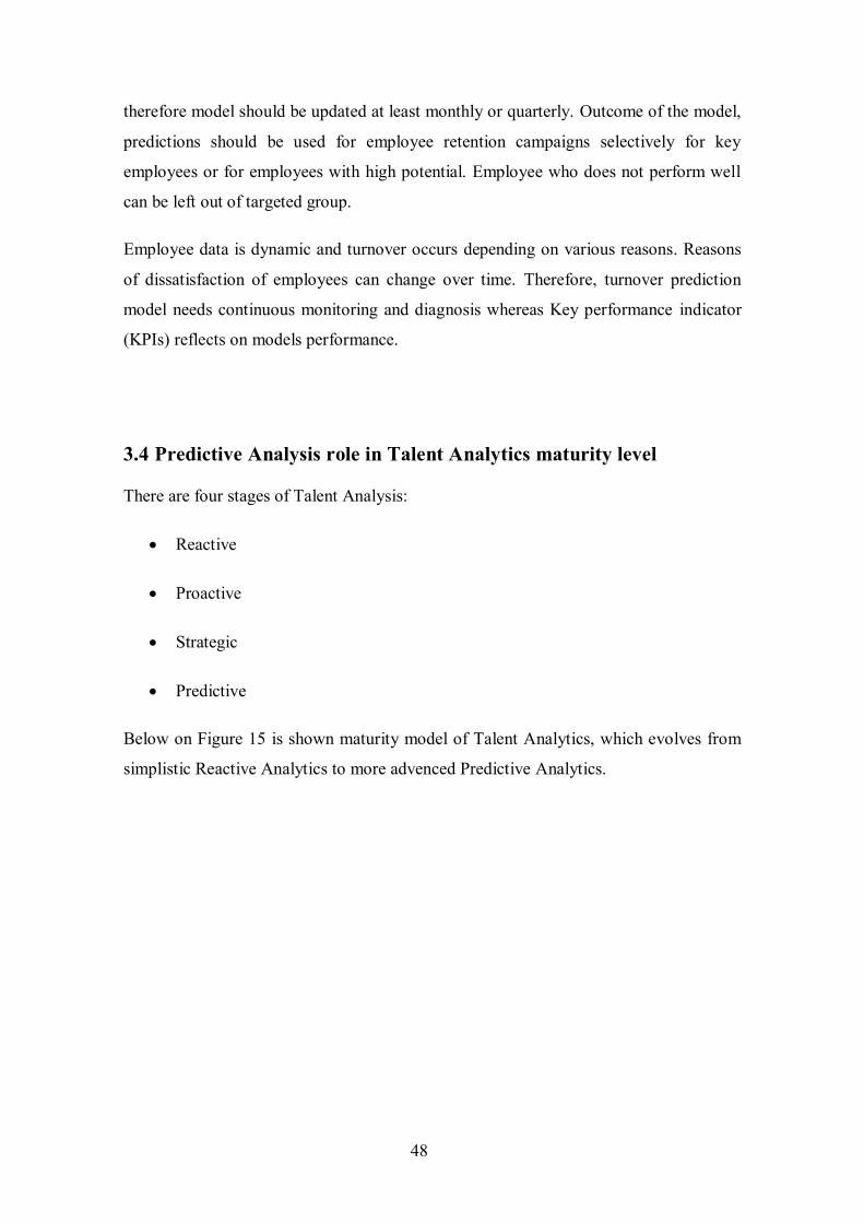
48

therefore model should be updated at least monthly or quarterly. Outcome of the model,

predictions should be used for employee retention campaigns selectively for key

employees or for employees with high potential. Employee who does not perform well

can be left out of targeted group.

Employee data is dynamic and turnover occurs depending on various reasons. Reasons

of dissatisfaction of employees can change over time. Therefore, turnover prediction

model needs continuous monitoring and diagnosis whereas Key performance indicator

(KPIs) reflects on models performance.

3.4 Predictive Analysis role in Talent Analytics maturity level

There are four stages of Talent Analysis:

Reactive

Proactive

Strategic

Predictive

Below on Figure 15 is shown maturity model of Talent Analytics, which evolves from

simplistic Reactive Analytics to more advenced Predictive Analytics.

49

Figure 15 Talent Analytics maturity model [61]

Fewer than 4% of organizations perform Predictive Analyses on their HR data, even

though HR processes are becoming more data driven [53] and there is demand for it

[62]. All of the companies that were studied by Deloitte went through four stages, they

were focusing on building scale, quality reporting and slowly moved up to building

predictive models. It is nearly impossible to build such analytics without strong

reporting infrastructure and clean, credible data.

3.5 HR Analysis in Swedbank

Almost two hundred years ago in Sweden First Savings bank was established, followed

by opening of first Swedish agricultural cooperative bank. Few decades after, in 1997

FöreningsSparbanken was established. Later on the bank expanded to Baltics. At the

beginning of 90’s Hansabank was founded in Estonia, few years later in Latvia and

Lithuania. FöreningsSparbanken AB changed name to Swedbank AB in 2006 [63].

Swedbank offers complete range of financial services to private and corporate

customers [64] [65]. Nowadays Swedbank has about eight million private customers

and over six thousand corporate customers over four countries [66]. By number of

50

customers Swedbank is largest bank in Sweden, Estonia, Latvia and Lithuania [67]. To

support business Swedbank has operations also in seven other countries, including

Norway, Finland, Denmark, Luxembourg, USA, China and South Africa [68]. For year

2016 Swedbank had 14 061 employees in all 11 countries [69].

Swedbank’s most valuable asset is its employees [70]. In Swedbanks’ annual report

2016, it is mentioned that ability of quickly adapting to changes is crucial for bank.

Development of digital technologies requires different set of skills from Swedbank

employees. In 2016 future skills and development needs in different business areas of

Swedbank was studied [69].

Since Swedbank employees are located in 11 countries, employee data comes from

different sources. In addition, for employee data management several HRIS tools are

used. Therefore, HR Analysis team in Swedbank faces challenge to rationalize and

unify data, so that standardized measures can be applied for all the regions. Currently

used HRIS tools in Swedbank do not have capability of Predictive analytics to be

implemented. HR reports built using such tools are descriptive, reflecting events

happening over indicated period of time. On top of such reports HR Analytics team

analyses data using HR KPIs, to measure achievement value of specific business

objective. Therefore, there was room to test Predictive Analysis for HR purposes and

evaluate how Machine Learning algorithms would perform for Swedbank employee

data.

51

4 Building predictive model

Since showing Swedbank data is a security issue, to show data preparation IBM

example dataset will be used [71]. However, result of Machine Learning algorithms will

be shown on Swedbank’s example.

For example dataset ‘Watson analytics sample data for HR employee attrition and

performance’ [72] has been selected. Example dataset contains information about

employees of a company including attrition attribute. Outcome of the analysis should be

the probability of attrition. In example dataset there are 36 variables, including the

outcome variable (attrition). The dataset has 1471 data observations in data file.

To predict employee turnover, we should predict who will leave. That is binomial

classification problem, where set of employees should be divided into two groups based

on some characteristics, ones with higher risk of attrition and ones with less.

Commonly used Machine Learning algorithms for binomial classification problem are:

decision trees, Random Forest, decision jungles, Bayesian networks, Neural Networks,

support vector machine and logistic regression [73], out of which bellow will be used

Random Forest, Neural Networks and Support Vector Machine.

4.1 Data preparation on example dataset

To reduce dimensionality only most relevant potential influencer variables will be

selected as predictors. In example dataset data is static not periodic, therefore data

preparation will be needed to be done once.

For Predictive Modelling user-driven approach will be used, meaning only strategically

selected subset of data will be used. Table 2 shows selected 18 features.

Since example dataset does not come from different sources there is no need to join

multiple tables and flatten file.

Also no dates and time sequences are being used explicitly. Dates were already rolled

up into durations in variable such as “Years since last promotion” and “Years at

company”.

52

Dataset is structured and presented in a tabular form. It includes behavioural,

demographic and attitudinal data. On Table 2 features has been categorized accordingly.

Table 2 Data Categorisation.

Behavioural Attitudinal Demographic

Years at Company Environment Satisfaction Age

Over Time Job Satisfaction Monthly Income

Performance Rating Work Life Balance Distance From Home

Years Since Last Promotion Work Life Balance Marital Status

Total Working Years Number of Companies Worked Education

Percent Salary Hike Relationship Satisfaction Gender

All of the demographic variables named above are qualitative variables, except age,

income and distance from home. While all of the behavioural and attitudinal variables

are qualitative.

Below on Table 3 is shown variable categorisation.

Table 3 Variable categorisation.

Numerical Categorical

Continuous Discrete Ordinal Nominal

Monthly Income Years at Company Environment Satisfaction Age

Distance From Home Years Since Last Promotion Job Satisfaction Over Time (has yes/no values)

Percent Salary Hike Number of Companies Worked Work Life Balance Marital Status

Total Working Years Performance Rating Education

Work Life Balance Gender

Relationship Satisfaction

There were few categorical variables in sample dataset. They were replaced by

numerical variable using pandas get_dummies function, which creates dummy indicator

variables. By indicating how many unique values specific variable has, variables that

needed dummy replace have been identified. If variable has too many unique values,

classifying values differently should be considered. For example, grouping some

answers in "other" value. On Figure 16 is shown identified number of unique values for

data variables.

53

Figure 16 Unique values for features.

All categorical features shown on Figure 16 were replaced with numerical values,

including ordinal variables such as job satisfaction. After using dummy replacements

there were 74 features in dataset.

For discovering missing values in dataset and for imputing them (in this case, replacing

them with median) sklearn.preprocessing.Imputer method was used.

To find out whether there is outlier in example dataset Tukey IQR approach has been

used. By calculating quartile one (Q1), quartile three (Q3) and inter quartile (Q3 − Q1)

upper and lower bound is indicated next way:

Lower Bound Q1 − 1.5 ∗ (Q3 − Q1) (9)

Upper Bound Q3 + 1.5 ∗ (Q3 − Q1) (10)

Values below or above lower (9) and upper bound (10) Upper Bound Q3 + 1.5 ∗

(Q3 − Q1) (10) are considered as outliers.

Multiplier 1.5 can be adjusted as needed.

There were some outliers found for ‘MonthlyIncome’ and ‘Age’ features. Outliers

were treated as missing values. Therefore they were changed to none values and

afterwards same imputer method was applied.

1

2

2

2

3

3

3

4

4

4

4

4

5

6

9

Over18

Gender

OverTime

PerformanceRating

BusinessTravel

Department

MaritalStatus

EnvironmentSatisfaction

JobInvolvement

JobSatisfaction

RelationshipSatisfaction

WorkLifeBalance

Education

EducationField

JobRole

54

On Figure 27 number of imputed outliers for features is shown. They were replaced

with median same way described above about treating missing values. On Figure 17 it is

shown how distribution of monthly income looks like after handling the outliers.

Figure 17 Distribution of monthly income

Figure 18 Outlier values (in blue) of monthly income

On Figure 18 red points represent values of monthly income after imputation of outlier

values, which are shown as blue points.

For detecting continuous variables next approach was used: if unique values for

variable was more than half of total number of values, such variable was considered as

continuous variable. On Table 4 is shown discovered continuous variables in sample

dataset. Although ‘EmployeeNumber’ is identifier, which means that it has unique value

for each employee. Therefore, it has high cardinality and should be removed

completely.

55

Table 4 Continuous variables

Feature name Unique values Total values

DailyRate 886 1470

EmployeeNumber 1470 1470

MontlyIncome 1238 1470

MontlyRate 1427 1470

For identification of skew direction scipy.stats.skew function has been used. If the result

is greater than zero skew is positive, if zero or close to zero it is a normal distribution

and if result is less than zero it is negative skew. Table 5 shows skew for discovered

continuous variables. For all of the variables except ‘MonthlyIncome’ skew is close to

zero. In case of monthly income there is a positive skew.

Table 5 Skewness of continuous variables

Variable Skew

DailyRate -0.0

EmployeeNumber 0.02

MonthlyIncome 1.29

MonthlyRate 0.02

On Figure 19 is clearly visible that there is positive skew in distribution of

‘MonthlyIncome’.

Figure 19 Distribution of MonthlyIncome

Since skew is positive, logarithmic transformation has been used for reducing skew.

56

Figure 20 Distribution of MonthlyIncome after logarithmic transformation

On Figure 20 it is clearly visible that after transformation skew has been reduced and

distribution has symmetrical bell curve.

Additionally, in the sample dataset interactions between variables has been identified

and added as new features. This technique is useful if the impact of two or more

features on the outcome is non-additive. Interactions within dummy variables created

earlier for replacing categorical variables will be always zero. Therefore, there will be

no additional features of interaction added for them. Since calculation of interactions is

computationally expensive operation, it is better to have domain knowledge and

calculate interactions only for selected variables. For combining features in python

itertools.combinations function has been used and for calculation of interaction

sklearn.preprocessing.PolynomialFeatures. There were 892 features after adding extra

features of interactions in sample data.

Afterwards to decrease dimensionality principal component analysis (PCA) algorithm

has been applied. In python sklearn.decomposition.PCA method has been used for

calculations.

Sklearn library for python has feature selection method for large set of features to avoid

risk of over-fitting and reduce computing time. Function

sklearn.feature_selection.SelectKBest requires number of features to be indicated. In

57

case of example data 20 features was indicated, since there is not enough number of

observations. But for Swedbank dataset all features has been used.

4.2 Modelling on Swedbank example

Given sample of Swedbank data contained 7 times more observations than IBM dataset.

It contained 15 features. Data preparation was done similar way as described above on

example dataset.

After pre-processing the data, three different Machine Learning models have been

applied. Random Forest, Multi-layer perceptron and Support vector machine was

selected algorithms, based on different approaches they use for prediction.

Each model first was configured and most suited parameters were chosen. For

evaluation sklearn.cross_validation.train_test_split was used. Dataset was randomly

split so that 70% was used for training and 30% for validation. Train-test split was

repeated several times and mean model accuracy was calculated.

After parameters were tuned, models were evaluated using 10-fold cross validation. For

evaluating model performances sklearn.metrics.roc_auc_score function was used,

which computes Area under the Curve (AUC) from prediction scores, the receiver

operating characteristic (ROC) curve.

Output of model was prediction of attrition for each employee, along with prediction

probability. For calculating prediction probabilities predict_proba function was used.

4.2.1 ROC_AUC

For evaluating model performances it is more convenient to use one metric.

Confusion Matrix of test dataset for prediction models will be:

Table 6 Confusion Matrix

Predicted class Employee Leaver

Actual class Employee 𝑒 𝑒̅ Leaver 𝑙 ̅ 𝑙

58

Where 𝑒 is number of correctly classified data object (called true positive), in this study

case correctly predicted number of employees. 𝑒̅ is number of misclassified employees

(false negatives). Analogically, 𝑙 ̅ is number of misclassified leavers (false positive) and

𝑙 is number of correctly predicted leavers (true negative).

From confusion matrix two metrics can be calculated:

𝑇𝑟𝑢𝑒 𝑝𝑜𝑠𝑖𝑡𝑖𝑣𝑒 𝑟𝑎𝑡𝑒 =𝑒

𝑒 + �̅� (11)

𝐹𝑎𝑙𝑠𝑒 𝑝𝑜𝑠𝑖𝑡𝑖𝑣𝑒 𝑟𝑎𝑡𝑒 =𝑙 ̅

𝑙+̅𝑙 (12)

ROC curve is plotted using true positive rate and false positive rate coordinates, shown

on Figure 21.

AUC calculates the area under the ROC curve.

Figure 21 Receiver operating characteristic example [74]

In this thesis for plotting a ROC curve probability of employee being classified as leaver

and actual class (target variable) will be used.

59

4.2.2 Tuning parameters of Random Forest Classifier

Random Forest model was trained using sklearn.ensemble.randomforestclassifier

function. For choosing best model parameters (hyper-parameters) grid search was

performed. In addition different values for parameters were looped and tested on model.

For Random Forest classifier maximum number of features used in each individual tree

can be specified [75]. By default if it will not be specified there is no restriction on

number of features. Initially there were 15 features in Swedbank dataset, but after

creating dummy variables, two ways interaction features and selecting most important

features using sklearn.feature_selection.SelectKbest function there were 164 features

available. Therefore from 1 to 164 possibilities of maximum number of features can be

used in each tree. After plotting iteration results it is visible that model performs better

if number of features used in each tree is higher than 20. Chosen value for max_features

is 118 because model accuracy is best.

Figure 22 max_features parameter for randomforestclassifier

Other than max_features, n_estimators is also important parameter for

randomforestclassifier function. It defines number of trees in random forest. More trees

there are, better the accuracy will be. However it will slow down the process [76]. By

default number of trees for randomforestclassifier function is ten. For evaluating model

performance 1 to 100 number of trees was tested. Results can be seen on Figure 25. It

does not improve much after 18, therefore 18 trees were selected.

60

For initializing minimum number of samples at leaf node of a decision tree

min_sample_leaf parameter should be initialized. Selected minimum number of samples

for leaf was 10. Testing results can be seen on Figure 26.

Other parameters like n_jobs for number of parallel processes, random_state and so on

can be initialized for making training easier and faster.

Tuning parameters is also possible using sklearn.model_selction.GridSearchCV

function. This function takes wide range of parameters and evaluates model for each

combination of parameters. Parameters selected using grid search led to better model

performance. Table 7 shows results.

Table 7 Selected parameters for Randomforestclassifier

Parameter Value

bootstrap True

min_samples_leaf 10

n_estimators 300

criterion 'entropy'

max_features 100

max_depth None

Average performance accuracy of models applied on test dataset is shown on Table 8.

Table 8 Performance results of differently tuned Randomforestclassifier

Model Average ROC_AUC

score Randomforestclassifier with default parameters 99.57% Randomforestclassifier with manually selected parameters using iteration 99.68% Randomforestclassifier with parameters selected using GridSearchCV 99.80%

Optimizing each of the parameters independently by iteratively assigning different

values did not yield as good results as grid search method. Grid search tests all of the

possible combinations of indicated values for parameters. Since best performance result

showed gird search algorithm it will be used for tuning parameters for Neural Networks

and Support vector machine as well.

61

4.2.3 Tuning parameters for Multi-Layer Perceptron

Grid search was used for tuning parameters for sklearn.neural_network.MLPClassifier

function. On first try tuned parameters showed worse result than parameters without

tuning. Results of first parameter tuned model can be seen on Table 9.

Table 9 MLPClassifier test results.

Model Average ROC_AUC

score

Training accuracy

Testing accuracy

MLPClassifier using default parameter values 79.35% 86.64% 85.67% MLPClassifier using tuned parameter values 77.20% 84.96% 84.12% Single perceptron with default parameters 79.09% 78.66%

In order to reduce variance in results, number of iterations for train-test split validation

has been increased to hundred. Additionally assigned grid values were refined

iteratively. Results can be seen on Table 10.

Table 10 MLPClassifier performance using tuned parameters

Model Average ROC_AUC

score

Training accuracy

Testing accuracy

MLPClassifier using default parameter values 78.26% 82.88% 82.26% MLPClassifier using tuned parameter values 77.91% 84.11% 83.27% MLPClassifier using tuned parameter values + tuned alpha

78.56% 81.81% 81.31%

For increasing accuracy of model with tuned parameters different possible values have

been tested iteratively. For parameter alpha results are shown on Figure 28, selected

value for alpha was 0.05.

Results for trying different values for max_iter are shown on Figure 29. Results for

hidden_layer_sizes are shown on Figure 30 and Figure 31. However on graphs is not

visible which values would give better result.

Parameters that showed best result are listed in Table 11.

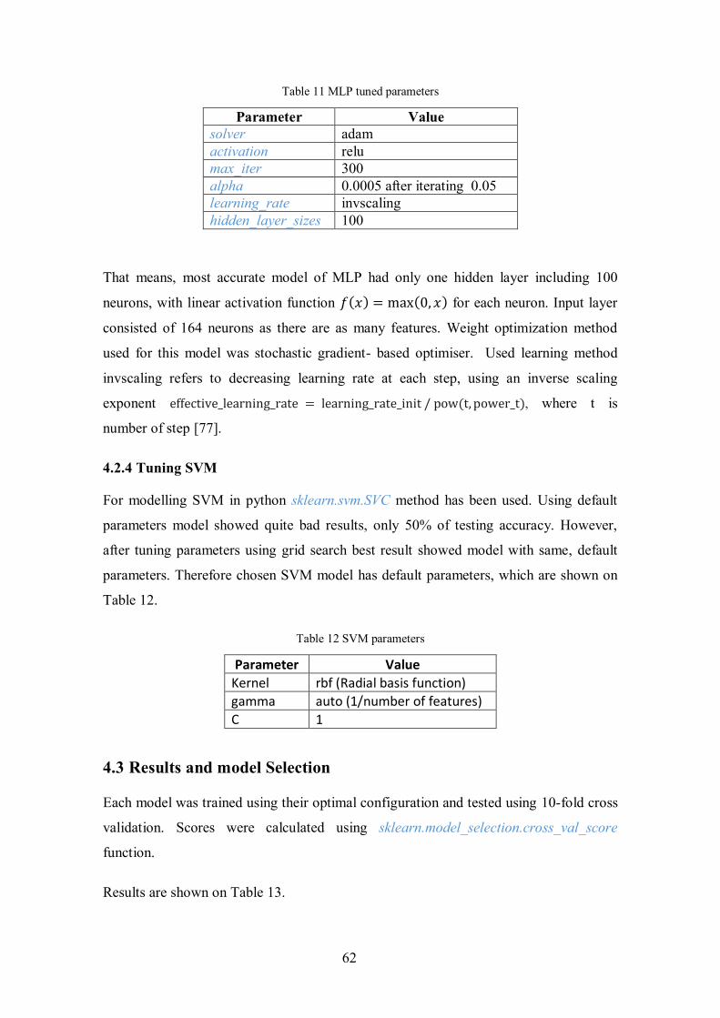
62

Table 11 MLP tuned parameters

Parameter Value solver adam activation relu max_iter 300 alpha 0.0005 after iterating 0.05 learning_rate invscaling hidden_layer_sizes 100

That means, most accurate model of MLP had only one hidden layer including 100

neurons, with linear activation function 𝑓(𝑥) = max(0, 𝑥) for each neuron. Input layer

consisted of 164 neurons as there are as many features. Weight optimization method

used for this model was stochastic gradient- based optimiser. Used learning method

invscaling refers to decreasing learning rate at each step, using an inverse scaling

exponent effective_learning_rate = learning_rate_init / pow(t, power_t), where t is

number of step [77].

4.2.4 Tuning SVM

For modelling SVM in python sklearn.svm.SVC method has been used. Using default

parameters model showed quite bad results, only 50% of testing accuracy. However,

after tuning parameters using grid search best result showed model with same, default

parameters. Therefore chosen SVM model has default parameters, which are shown on

Table 12.

Table 12 SVM parameters

Parameter Value

Kernel rbf (Radial basis function)

gamma auto (1/number of features)

C 1

4.3 Results and model Selection

Each model was trained using their optimal configuration and tested using 10-fold cross

validation. Scores were calculated using sklearn.model_selection.cross_val_score

function.

Results are shown on Table 13.

63

Table 13 Model selection

Model Mean cross validation score

Random Forest 98.62%

MLP 79.14%

SVM 71.49%

Random Forest showed best results on example dataset as well.

Afterwards trained Random Forest model was applied to employee dataset. Predicted

values and probabilities were then exported to excel file. In addition, using function

sklearn.tree.export_graphviz decision trees (used in random forest) were extracted. On

Figure 23 is shown branch of one of the decision trees of Random Forest classifier on

IBM example dataset. Different labels are colour coded. Intensity of colour shows

number of samples in that branch.

Figure 23 Branch of decision tree.

Also for better understanding which variables had more influence on outcome

feature_importances_ function was used. On Figure 24 is shown most important

features for example dataset. It can be seen that interactions between features had more

influence on outcome than initial features. For example, feature

64

‘MonthlyIncome_OverTime_No’ holds monthly income values of employees who do

not work overtime.

Figure 24 Feature importance

To conclude, Random Forest classifier performed better than other tested models, on

both Swedbank and IBM sample datasets. Therefore Random Forest model has been

used to predict employee turnover in Swedbank. Prediction results have been saved in

flat file, including prediction probabilities for each employee. In addition, for

interpretation of the decision path, decision trees were represented as graphs.

Furthermore, feature importance has been evaluated to better understand variables that

influenced the decision most. For IBM example dataset such influencers were monthly

income, age, hourly rate, working years, distance from home, salary hike, marital status

and job level, all in correlation with over time.

MonthlyIncome_OverTime_No

MonthlyIncome_OverTime_Yes

Age_OverTime_No

HourlyRate_OverTime_Yes

TotalWorkingYears_OverTime_No

DistanceFromHome_OverTime_Yes

PercentSalaryHike_OverTime_No

PercentSalaryHike_OverTime_Yes

MaritalStatus_Single_OverTime_Yes

JobLevel_OverTime_No

OverTime_Yes_PerformanceRating_Excellent

65

5 Summary

The aim of the thesis was to apply Predictive Analysis methodology on Swedbanks’ HR

data, in order to analyse the use of predictive analysis for HR. Author of the thesis is

employed in Swedbank in Group HR Analysis team and was aware of available room

for further improving HR Analytics using Predictive Analysis. Chosen metric for

prediction was employee turnover, because of its high importance for organization.

Thus goal of the thesis was predicting employee turnover.

In this work, data preparation has been done on both example and Swedbank datasets.

Example dataset was used for demonstrating methods used for cleaning and preparing

data. First of all, Swedbank data from multiple sources has been gathered and unified.

Then missing values has been imputed, outliers have been removed and skew has been

reduced.

Afterwards parameters for selected Machine Learning algorithms have been tuned using

different methodologies. Later, on pre-processed employee data different machine

learning algorithms have been applied and algorithm with best prediction accuracy has

been selected.

Eventually model has been applied to current employee dataset and outcome predictions

along with prediction probabilities were saved in flat file. In addition, for understanding

how decision was made, the model was interpreted by plotting decision graph and

identifying most important features.

Outcome of the thesis is Swedbank employee turnover prediction. The aim is reached

as application of model was successful. Using outcome flattened file turnover rate can

be estimated or for key employees retention actions can be applied.

To improve prediction results in the future other features can be added to dataset.

Missing values can be eliminated by collecting respective data. More Machine Learning

methods can be applied and evaluated.

66

References

[1] Pankaj Ajit Rohit Punnoose, "Prediction of Employee Turnover in Organizations using Machine Learning Algorithms".

[2] simpelearn. [Online]. https://www.simplilearn.com/data-science-vs-big-data-vs-data-analytics-article

[3] Investopedia. [Online]. http://www.investopedia.com/terms/d/datamining.asp [4] Sas. [Online]. https://www.sas.com/en_us/insights/analytics/big-data-

analytics.html [5] Predictive Analytics Today website. [Online].

http://www.predictiveanalyticstoday.com/what-is-predictive-analytics/ [6] tdwi. [Online]. https://tdwi.org/articles/2007/05/10/predictive-analytics.aspx [7] Business Dictionary. [Online].

http://www.businessdictionary.com/definition/business-intelligence-BI.html [8] ischool. [Online]. https://ischool.syr.edu/infospace/2013/11/13/using-predictive-

analytics-to-understand-your-business/ [9] beyondcore. [Online].

http://www.impactanalytix.com/samples/DataPrepforPredictiveAnalytics.pdf [10] quora. [Online]. https://www.quora.com/What-is-the-difference-between-static-

data-and-streaming-data-What-are-the-examples [11] variables. [Online].

http://www.abs.gov.au/websitedbs/a3121120.nsf/home/statistical+language+-+what+are+variables

[12] Big data analytics. [Online]. http://searchbusinessanalytics.techtarget.com/definition/big-data-analytics

[13] unstructured data. [Online]. http://www.councilscienceeditors.org/wp-content/uploads/v37n2p40-44.pdf

[14] UIM. [Online]. https://www.ibm.com/support/knowledgecenter/SSEPGG_9.5.0/com.ibm.datatools.datamining.doc/c_ta_uima_concepts.html

[15] outlier. [Online]. http://mathworld.wolfram.com/Outlier.html [16] skew. [Online]. http://www.managedfuturesinvesting.com/managed-

futures/news/aisource-news/2015/10/13/what-is-skewness [17] GKStatsBookSkewness. [Online].

http://growingknowing.com/GKStatsBookSkewness.php [18] brownmath. [Online]. https://brownmath.com/stat/shape.htm [19] skew reduction. [Online].

https://blackboard.swan.ac.uk/bbcswebdav/institution/IntroductoryMedicalStatistics/page_10.htm

67

[20] high cardinality. [Online]. https://www.researchgate.net/publication/272522918_Including_High-Cardinality_Attributes_in_Predictive_Models_a_Case_Study_in_Churn_Prediction_in_the_Energy_Sector

[21] Pugliese Amedeo, Recker Jan Mertens Willem, Quantitative Data Analysis. [22] pca. [Online]. http://sebastianraschka.com/Articles/2015_pca_in_3_steps.html [23] machine learning algorithms. [Online]. http://machinelearningmastery.com/a-

tour-of-machine-learning-algorithms/ [24] Volodymyr Mnih et al., "Playing Atari with Deep Reinforcement Learning,"

CoRR, 2013. [Online]. https://www.cs.toronto.edu/~vmnih/docs/dqn.pdf [25] clustering. [Online]. http://dataaspirant.com/2016/09/24/classification-clustering-

alogrithms/ [26] lecture. [Online]. http://www.stat.cmu.edu/~cshalizi/350/lectures/19/lecture-

19.pdf [27] sckitlearn. [Online]. http://scikit-learn.org/stable/modules/cross_validation.html [28] NN. [Online].

https://www.tutorialspoint.com/artificial_intelligence/artificial_intelligence_neural_networks.htm

[29] yhat. [Online]. http://blog.yhat.com/posts/random-forests-in-python.html [30] Trevor Hastie, The Elements of Statistical Learning. [31] Robert Tibshirani, Jerome Friedma Trevor Hastie, The elements of statistical

learning. [32] perceptron. [Online]. https://appliedgo.net/perceptron/ [33] MLP. [Online].

http://neuroph.sourceforge.net/tutorials/MultiLayerPerceptron.html [34] Adrian J. Shepherd, Second-Order Methods for Neural Networks_ Fast and

Reliable Training Methods for Multi-Layer Perceptrons. [35] SVM. [Online]. http://scikit-learn.org/stable/modules/svm.html [36] SVM2. [Online]. https://www.analyticsvidhya.com/blog/2015/10/understaing-

support-vector-machine-example-code/ [37] (2016, June) KDnuggets. [Online]. http://www.kdnuggets.com/2016/06/r-python-

top-analytics-data-mining-data-science-software.html [38] Burthcworks. [Online]. http://www.burtchworks.com/2016/07/13/sas-r-python-

survey-2016-tool-analytics-pros-prefer/ [39] R4stats. [Online]. http://r4stats.com/articles/popularity/ [40] John Fox and Robert Andersen. (2005, January) Using the R Statistical

Computing Environment to Teach Social Statistics Courses. [Online]. http://www.unt.edu/rss/Teaching-with-R.pdf

[41] R Home page. [Online]. https://www.r-project.org/about.html [42] Alan Brown. LinkedIn. [Online]. https://www.linkedin.com/pulse/forecasting-

facebooks-prophet-alan-brown [43] SAS Homepage. [Online]. https://support.sas.com/software/ [44] NumPy homepage. [Online]. http://www.numpy.org/ [45] Pandas homepage. [Online]. http://pandas.pydata.org/

68

[46] Scikit-learn homepage. [Online]. http://scikit-learn.org/ [47] TensorFlow homepage. [Online]. https://www.tensorflow.org/ [48] pyzo. [Online]. http://www.pyzo.org/python_vs_matlab.html [49] mat2. [Online]. https://se.mathworks.com/solutions/data-analytics.html [50] [Online]. https://se.mathworks.com/help/matlab/mapreduce.html [51] HR. [Online]. https://2012books.lardbucket.org/books/beginning-management-of-

human-resources/s05-the-role-of-human-resources.html [52] paper HRM. [Online].

http://samples.jbpub.com/9781449653293/27829_CH01_003_032.pdf [53] HR. [Online]. https://dupress.deloitte.com/dup-us-en/deloitte-review/issue-

14/dr14-datafication-of-hr.html [54] HR analytics. [Online].

http://searchfinancialapplications.techtarget.com/definition/human-resources-analytics

[55] Mary B. Young, "Strategic Workforce Planning". [56] turnover formula. [Online]. https://www.thebalance.com/employee-turnover-

2275788 [57] smallbusiness. [Online]. http://smallbusiness.chron.com/employee-turnover-vs-

attrition-15846.html [58] turnover causes. [Online]. http://smallbusiness.chron.com/causes-effects-high-

low-staff-turnover-33939.html [59] Turnover blog. [Online]. http://www.inostix.com/blog/en/4-challenges-with-

predictive-employee-turnover-analytics/ [60] turnover chalanges. [Online]. http://www.inostix.com/blog/en/4-challenges-with-

predictive-employee-turnover-analytics/ [61] bersin. [Online]. http://www.bersin.com/Lexicon/Details.aspx?id=15302 [62] Predictive workforce turnover. [Online]. http://www.talentanalytics.com/blog/the-

beginners-guide-to-predictive-workforce-analytics/ [63] swedbank. [Online]. https://www.swedbank.com/about-swedbank/our-

history/swedbank-and-the-savings-banks/ [64] Swedbank corporate. [Online]. https://www.swedbank.com/corporate/ [65] Swedbank Private. [Online]. https://www.swedbank.com/private/ [66] Swedbank Facts. [Online]. https://www.swedbank.com/about-swedbank/quick-

facts/ [67] Swedbank investors. [Online]. https://www.swedbank.com/investor-

relations/#&panel1-7 [68] Swedbank facts. [Online]. https://www.swedbank.com/investor-relations/quick-

facts/ [69] Annual report 2016. [Online].

https://www.swedbank.com/idc/groups/public/@i/@sbg/@gs/@ir/documents/financial/cid_2256557.pdf

[70] Swedbank employees. [Online]. https://www.swedbank.com/career/employees/ [71] example dataset. [Online]. https://www.ibm.com/communities/analytics/watson-

analytics-blog/hr-employee-attrition/

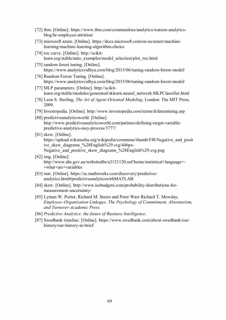
69

[72] ibm. [Online]. https://www.ibm.com/communities/analytics/watson-analytics-blog/hr-employee-attrition/

[73] microsoft azure. [Online]. https://docs.microsoft.com/en-us/azure/machine-learning/machine-learning-algorithm-choice

[74] roc curve. [Online]. http://scikit-learn.org/stable/auto_examples/model_selection/plot_roc.html

[75] random forest tuning. [Online]. https://www.analyticsvidhya.com/blog/2015/06/tuning-random-forest-model/

[76] Random Forest Tuning. [Online]. https://www.analyticsvidhya.com/blog/2015/06/tuning-random-forest-model/

[77] MLP parameters. [Online]. http://scikit-learn.org/stable/modules/generated/sklearn.neural_network.MLPClassifier.html

[78] Leon S. Sterling, The Art of Agent-Oriented Modeling. London: The MIT Press, 2009.

[79] Investopedia. [Online]. http://www.investopedia.com/terms/d/datamining.asp [80] predictiveanalyticsworld. [Online].

http://www.predictiveanalyticsworld.com/patimes/defining-target-variable-predictive-analytics-easy-process/3777/

[81] skew. [Online]. https://upload.wikimedia.org/wikipedia/commons/thumb/f/f8/Negative_and_positive_skew_diagrams_%28English%29.svg/446px-Negative_and_positive_skew_diagrams_%28English%29.svg.png

[82] img. [Online]. http://www.abs.gov.au/websitedbs/a3121120.nsf/home/statistical+language+-+what+are+variables

[83] mat. [Online]. https://se.mathworks.com/discovery/predictive-analytics.html#predictiveanalyticswithMATLAB

[84] skew. [Online]. http://www.isobudgets.com/probability-distributions-for-measurement-uncertainty/

[85] Lyman W. Porter, Richard M. Steers and Peter Warr Richard T. Mowday, Employee–Organization Linkages. The Psychology of Commitment, Absenteeism, and Turnover-Academic Press.

[86] Predictive Analytics: the future of Business Intelligence. [87] Swedbank timeline. [Online]. https://www.swedbank.com/about-swedbank/our-

history/our-history-in-brief/

70

Appendix 1 – Additional Figures

Figure 25 n_estimators parameter for randomforestclassifier

Figure 26 min_sample_leaf parameter for randomforestclassifier

71

Figure 27 Replaced outliers

Figure 28 alpha (1/Value of parameter) parameter for MLPClassifier

344

327

326

303

292

289

287

284

282

280

277

276

259

238

226

226

170

159

153

150

145

144

132

131

114

107

104

102

85

83

WorkLifeBalance_Good

MaritalStatus_Divorced

JobRole_Sales Executive

RelationshipSatisfaction_Medium

JobRole_Research Scientist

JobSatisfaction_Low

EnvironmentSatisfaction_Medium

EnvironmentSatisfaction_Low

Education_College

JobSatisfaction_Medium

BusinessTravel_Travel_Frequently

RelationshipSatisfaction_Low

JobRole_Laboratory Technician

TrainingTimesLastYear

PerformanceRating_Outstanding

PerformanceRating_Excellent

Education_Below College

EducationField_Marketing

WorkLifeBalance_Best

BusinessTravel_Non-Travel

JobRole_Manufacturing Director

JobInvolvement_Very High

EducationField_Technical Degree

JobRole_Healthcare Representative

MonthlyIncome

YearsSinceLastPromotion

YearsAtCompany

JobRole_Manager

StockOptionLevel

JobRole_Sales Representative

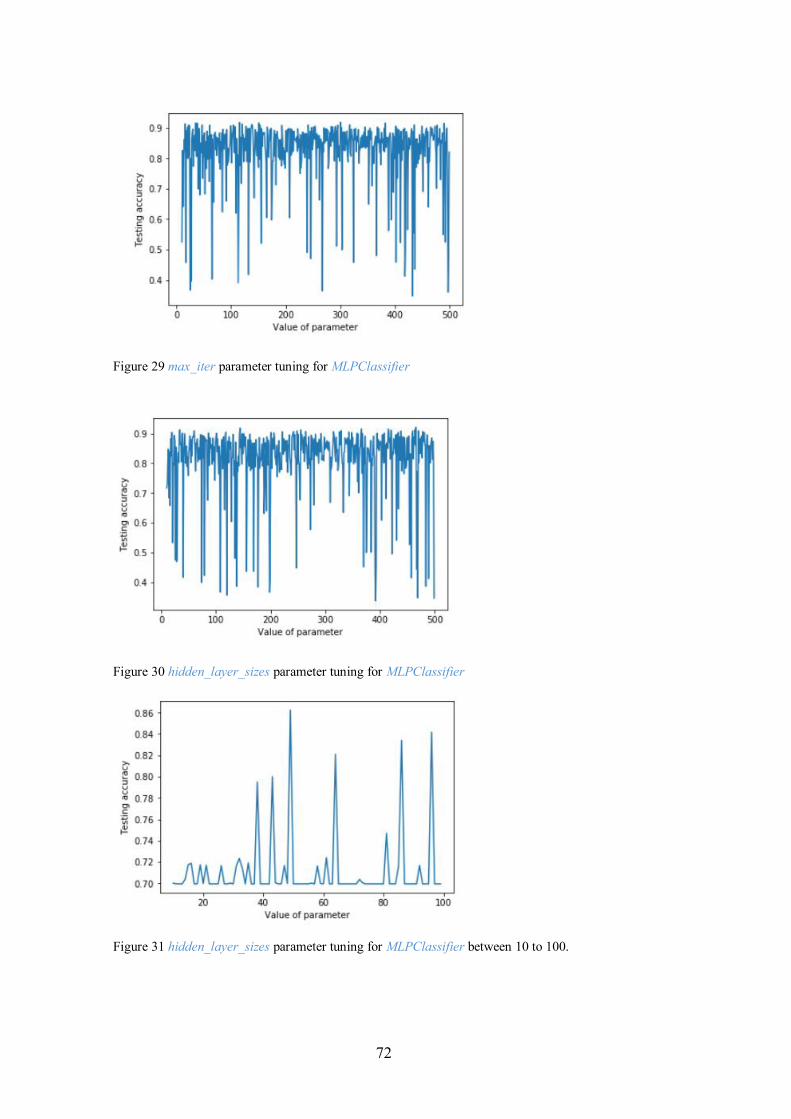
72

Figure 29 max_iter parameter tuning for MLPClassifier

Figure 30 hidden_layer_sizes parameter tuning for MLPClassifier

Figure 31 hidden_layer_sizes parameter tuning for MLPClassifier between 10 to 100.

73

Appendix 2 – Python Code

Categorical variables: def dummy_df(df,dummy_list):

for x in dummy_list:

dummies=pd.get_dummies(df[x],prefix=x, dummy_na=False)

df=df.drop(x,1)

df=pd.concat([df,dummies], axis=1)

return df

dummy_list=[]

val=[]

for col in X.columns:

if X[col].dtypes == 'object':

unique=len(X[col].unique())

val.append(unique)

dummy_list.append(col)

print(" Feature'{col}' has {unique} unique values".format(c

ol=col, unique=unique))

X=dummy_df(X,dummy_list)

Missing values: #imputing missing values

imp= Imputer(missing_values='NaN', strategy='median', axis=0)

imp.fit(X)

X=DataFrame(data=imp.transform(X), columns=X.columns)

# there should not be any missing values

X.isnull().sum().sort_values(ascending=False).head()

Outliers: def find_outliers(x):

q1 = np.percentile(x, 25)

q3 = np.percentile(x, 75)

iqr = q3-q1

low = q1 - 1.5*iqr

top = q3 + 1.5*iqr

outliers = list(x.index[(x < low)|(x > top)])

return outliers

for col in X.columns:

outliers = find_outliers(X[col])

# make outliers as missing

for i in outliers:

X.loc[i,col]=None

Continuous variables: #discover continuous varibales

var=[]

for col in X.columns:

unique=len(X[col].unique())

if unique>len(X[col])/5:

var.append(col)

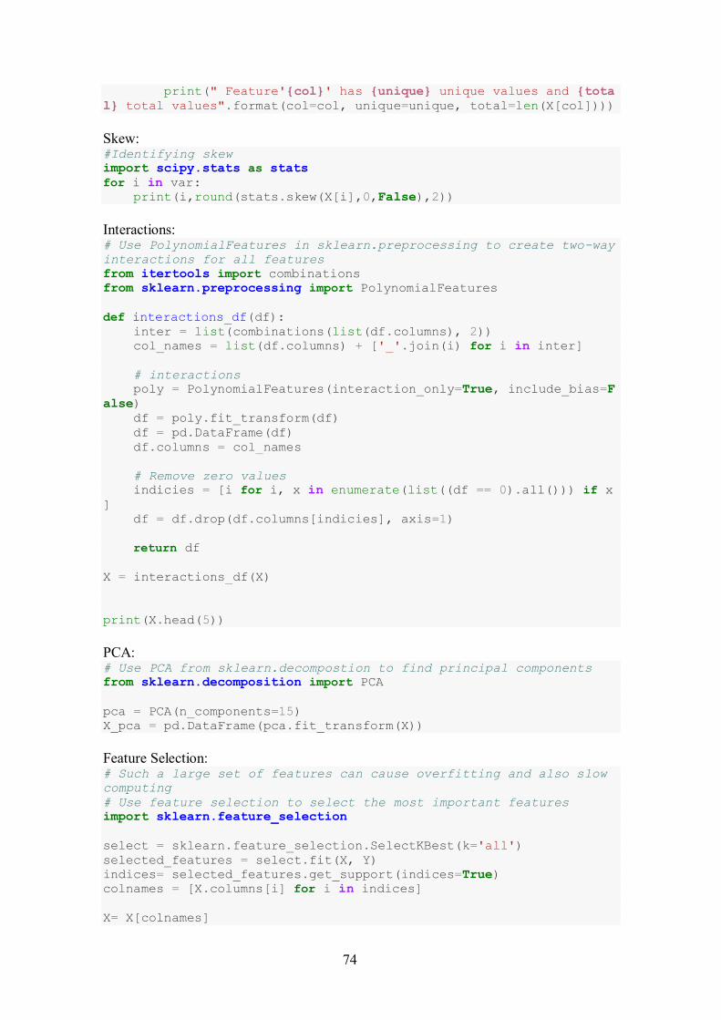
74

print(" Feature'{col}' has {unique} unique values and {tota

l} total values".format(col=col, unique=unique, total=len(X[col])))

Skew: #Identifying skew

import scipy.stats as stats

for i in var:

print(i,round(stats.skew(X[i],0,False),2))

Interactions: # Use PolynomialFeatures in sklearn.preprocessing to create two-way

interactions for all features

from itertools import combinations

from sklearn.preprocessing import PolynomialFeatures

def interactions_df(df):

inter = list(combinations(list(df.columns), 2))

col_names = list(df.columns) + ['_'.join(i) for i in inter]

# interactions

poly = PolynomialFeatures(interaction_only=True, include_bias=F

alse)

df = poly.fit_transform(df)

df = pd.DataFrame(df)

df.columns = col_names

# Remove zero values

indicies = [i for i, x in enumerate(list((df == 0).all())) if x

]

df = df.drop(df.columns[indicies], axis=1)

return df

X = interactions_df(X)

print(X.head(5))

PCA: # Use PCA from sklearn.decompostion to find principal components

from sklearn.decomposition import PCA

pca = PCA(n_components=15)

X_pca = pd.DataFrame(pca.fit_transform(X))

Feature Selection: # Such a large set of features can cause overfitting and also slow

computing

# Use feature selection to select the most important features

import sklearn.feature_selection

select = sklearn.feature_selection.SelectKBest(k='all')

selected_features = select.fit(X, Y)

indices= selected_features.get_support(indices=True)

colnames = [X.columns[i] for i in indices]

X= X[colnames]

75

X.columns

Train-test split: from sklearn.cross_validation import train_test_split

X_train, X_test, Y_train, Y_test = train_test_split(X, Y, train_siz

e=0.70, random_state=1)

RF grid search example: from sklearn.model_selection import GridSearchCV

X_train, X_test, Y_train, Y_test = train_test_split(X, Y, train_siz

e=0.70, random_state=1)

tuned_parameters={"n_estimators": [1,100,300],

"max_depth":[3,None],

"max_features":[1,100,118,164],

"min_samples_leaf":[1,10,100],

"bootstrap":[True,False],

"criterion":["gini","entropy"]}

clf=RandomForestClassifier()

grid_search=GridSearchCV(clf, param_grid=tuned_parameters)

grid_search.fit(X_train,Y_train)

print(grid_search.best_params_)

RF evaluation: sum_err_train = 0

sum_err_test = 0

sum_auc = 0

#split data into train and test datasets and iterate

for i in range(10):

# split

X_train, X_test, Y_train, Y_test = train_test_split(X, Y, train

_size=0.70, random_state=1)

# train

clf =RandomForestClassifier(bootstrap = False, min_samples_leaf

=1, n_estimators=100, criterion='entropy', max_features=10, max_dep

th= None)

clf.fit(X_train, Y_train)

clf.predict(X_test)

preds = clf.predict(X_test)

# evaluate

y_hat = [x[1] for x in clf.predict_proba(X_test)]

auc = roc_auc_score(Y_test, y_hat)

train_pred = clf.predict(X_train)

sum_err_train += float(sum(abs(train_pred - Y_train)))

sum_err_test += float(sum(abs(preds - Y_test)))

sum_auc +=auc

train_acc = 1 - sum_err_train / (10 * len(Y_train))

test_acc = 1 - sum_err_test / (10 * len(Y_test))

auc_acc = sum_auc / 10

print('Average training accuracy %.2f%%' % (train_acc * 100))

76

print('Average testing accuracy %.2f%%' % (test_acc * 100))

print('Average perfprmance test accuracy %.2f%%' % (auc_acc * 100))

K fold: from sklearn.cross_validation import KFold,cross_val_score

from sklearn.neural_network import MLPClassifier

from sklearn.svm import SVC

k_fold = KFold(len(Y), n_folds=10, shuffle=True, random_state=0)

clf1 = RandomForestClassifier(bootstrap = True, min_samples_leaf=10

, n_estimators=300, criterion='entropy', max_features=100, max_dept

h= None)

clf2 = MLPClassifier(hidden_layer_sizes=(100,), activation='relu',

max_iter= 300, alpha=0.05, solver= 'adam', learning_rate= 'invscal

ing')

clf3 = SVC()

result1=cross_val_score(clf1, X, Y, cv=k_fold, n_jobs=1)

result2=cross_val_score(clf2, X, Y, cv=k_fold, n_jobs=1)

result3=cross_val_score(clf3, X, Y, cv=k_fold, n_jobs=1)

print (result1.mean())

print (result2.mean())

print (result3.mean())

Writing into excel file: Z= DataFrame()

Z['ID']=xlsxdata['person_id']

Z['Attrition']= xlsxdata['Attrition']

clf1.fit(X,Y)

t1=[x[1] for x in clf1.predict_proba(X)]

t0=[x[0] for x in clf1.predict_proba(X)]

p=clf1.predict(X)

Z['probability-employee']=t0

Z['probability-leaver']=t1

Z[' predicted label']=p

Z.to_excel('results.xlsx', sheet_name='results', index=False)

Feature importance: importance=list(zip(X.columns,clf1.feature_importances_))

sorted(importance, key=lambda l:l[1], reverse=True)

Interpreting first tree of Random Forest: dot_data = tree.export_graphviz(clf1.estimators_[0],

out_file=None,

feature_names=X.columns,

class_names=Y.name,

filled=True, rounded=True,

special_characters=True)

graph = pydotplus.graph_from_dot_data(dot_data)

Image(graph.create_png())