Embed Size (px)
Citation preview
i
Predictive Ability of Current Earnings and Cash flows
Percy Gumbi
12112420
A research project submitted to the Gordon Institute of Business Science, University of Pretoria,
in partial fulfillment of the requirements for the degree of Master of Business Administration.
26 September 2012
Copyright © 2013, University of Pretoria. All rights reserved. The copyright in this work vests in the University of Pretoria. No part of this work may be reproduced or transmitted in any form or by any means, without the prior written permission of the University of Pretoria.
©© UUnniivveerrssiittyy ooff PPrreettoorriiaa
ii
ABSTRACT
This research investigated the ability of current earnings and cash flows to predict future cash
flows and future share prices. The investigation was conducted used financial information of
JSE listed companies over a period between 2001 and 2011. The objectives of the research were
to establish the predictive ability of current earnings and cash flows on future cash flows and
share prices. This study was motivated by the findings of Kim and Kross (2005) where they
consolidated the earlier findings by Collins et al. (1997) and Dechow et al. (1998).
It was predetermined that the study would add to the body of knowledge in financial statements
analysis and the application of earnings and cash flows as the predictive financial variables,
Earnings are regarded as an essential measure of company of company‘s performance and cash
flows from operations as a measure of the company‘s ability to generate cash flows from their
operations. It was noted that investors do study and analyse these financial elements when
investment decisions are made (Higgins, 2009; De Fond and Hung, 2003).
It was found that earnings did not have the predictive ability on future cash flows but proved to
possess high predictive power over future share prices. The results were not in agreement with
the previous studied on the same subject. The average of R-square on current earnings ability to
predict future cash flows were R2=0.27 and 0.38 in the long run and short run, respectively. The
predictive ability on future share prices were R2=0.44 and 0.54 in the long and short run,
respectively. Current cash flows on the hand indicated low predictive ability on future share
price where the average R2=0.24 and 0.33 in the long and short run respectively. The predictive
ability on current cash flows over future cash flows proved to be higher, which was not
consistent with the previous researchers. The average R2 were 0.44 and 0.46 in the long and
short run. It was noted that these financial elements proved to possess higher predictive abilities
in the short run.
Keywords: Earning, Cash flows; JSE Predictive, Regression analysis

iii
DECLARATION
I declare that this research project is my own work. It is submitted in partial fulfilment of the
requirements for the degree of Master of Business Administration at the Gordon Institute of
Business Science, University of Pretoria. It has not been submitted before for any degree or
examination in any other University. I further declare that I have obtained the necessary
authorisation and consent to carry out this research.
The name and the original signature of the student and the date should follow the declaration.
_________________________ ___________________
Percy Gumbi Date

iv
ACKNOWLEDGEMENTS
Firstly, I wish to acknowledge in a very thankful manner, my Heavenly Father who has made it
possible for me to go this far with my studies in the face of turbulence that I experienced during
course of this research.
I also wish to thank my supervisor, Mr Max Mackenzie who went beyond the call of duty of
being a supervisor but an inspiration and the support structure that one needed. I am very
grateful for the support and parting of his knowledge that made my research project not being a
tedious one.
My gratitude also goes to the Information Specialists, Monica and Patience for their assistance
with the retrieval of articles to referencing coaching sessions. My hearts also goes to Shirls for
being supportive since joining GIBS and thank her for her supporting role and at times for
providing a ―shoulder to cry on‖. I also thank the friendship that I established during the course
of the study, in particular my FT MBA class, you guys are great.
Last but not least, to my dearest wife Babalwa for being a pillar of my strength. I thank her for
her understanding during the last eighteen months being away from home. I also thank my three
wonderful kids, Olwethu, Lwandile and Uthando for their understanding when ―Papa‖ was away
for most of the time. I wish to assure them that the worst is over and now forward we will have
ample time of fun and games.
Thanks to GIBS management for the privilege to be associated with such an innovative and
forward thinking institution.
v
TABLE OF CONTENTS
ABSTRACT .......................................................................................................................................... ii
DECLARATION ................................................................................................................................... iii
ACKNOWLEDGEMENTS ..................................................................................................................... iv
1. BACKGROUND AND RESEARCH PROBLEM....................................................................................2
1.1 INTRODUCTION ............................................................................................................................. 2
1.2 RESEARCH PROBLEM ..................................................................................................................... 2
1.3 EARNINGS AND CASH FLOW ......................................................................................................... 4
1.4 OBJECTIVES ................................................................................................................................... 5
1.5 SCOPE OF THE RESEARCH PROBLEM ............................................................................................ 6
2. LITERATURE REVIEW ...................................................................................................................8
2.1 INTRODUCTION ............................................................................................................................. 8
2.2 EARNINGS ABILITY TO PREDICT FUTURE CASH FLOWS ................................................................. 8
2.3 CASH FLOW ABILITY TO PREDICT FUTURE CASH FLOWS ............................................................ 13
2.4 EARNINGS AND CASH FLOWS AS PREDICTORS OF FUTURE SHARE PRICE .................................. 18
2.4.1 EARNINGS AS THE PREDICTOR OF FUTURE SHARE PRICE ................................................... 18
2.4.2 CASH FLOW AS THE PREDICTOR OF FUTURE SHARE PRICE ................................................ 21
2.5 THE MODELS ............................................................................................................................... 24
2.5.1 BACKGROUND ..................................................................................................................... 24
2.5.2 CURRENT YEAR EARNINGS ABILITY TO PREDICT FUTURE CASH FLOW MODELS ................ 25
2.5.3 CURRENT YEAR CASH FLOWS’ ABILITY TO PREDICT FUTURE CASH FLOW MODEL............. 27
2.5.4 CURRENT EARNINGS ABILITY TO PREDICT FUTURE SHARE PRICE MODEL ......................... 28
2.5.5 CURRENT CASH FLOWS ABILITY TO PREDICT FUTURE SHARE PRICE MODEL ..................... 29
2.6 CONCLUSION ............................................................................................................................... 30
3. RESEARCH QUESTIONS AND HYPOTHESIS .................................................................................. 32
3.1 RESEARCH HYPOTHESIS .............................................................................................................. 32
3.2 CONSISTENCY MATRIX ................................................................................................................ 33
4. RESEARCH METHODOLOGY ....................................................................................................... 35
4.1 RATIONALE OF THE RESEARCH METHOD .................................................................................... 35
4.2 UNIT OF ANALYSIS ....................................................................................................................... 35
4.3 POPULATION ............................................................................................................................... 36
vi
4.4 SAMPLING METHOD AND SIZE .................................................................................................... 37
4.5 DATA COLLECTION ...................................................................................................................... 38
4.6 DATA ANALYSIS (STATISTICS) ...................................................................................................... 40
4.6.1 ABILITY OF EARNINGS AND CASH FLOWS PRECICT FUTURE CASH FLOWS AND FUTURE
SHARE PRICES IN THE LONG RUN ....................................................................................................... 41
4.6.2 ABILITY OF EARNINGS AND CASH FLOWS PRECICT FUTURE CASH FLOWS AND FUTURE
SHARE PRICES IN THE SHORT- RUN ..................................................................................................... 42
4.6.3 TESTING THE COEFICIENT OF CORRELATION ...................................................................... 43
4.7 LIMITATIONS ............................................................................................................................... 44
5. RESULTS ................................................................................................................................... 46
5.1 INTRODUCTION ........................................................................................................................... 46
5.2 DESCRIPTIVE STATISTICS ............................................................................................................. 46
5.3 RESEARCH HYPOTHESIS RESULTS ................................................................................................ 51
5.3.1 RESEARCH HYPOTHESIS 1 .................................................................................................... 51
5.3.2 TEST OF COEFFICIENT OF CORRELATION ............................................................................ 63
6. DISCUSSION.............................................................................................................................. 68
6.1 INTRODUCTION ........................................................................................................................... 68
6.2 CURRENT EARNINGS’ ABILITY TO PREDICT FUTURE CASH FLOWS ............................................. 69
6.3 CURRENT CASH FLOWS’ABILITY TO PREDICT FUTURE CASH FLOWS .......................................... 71
6.4 CURRENT EARNINGS’ ABILITY TO PREDICT FUTURE SHARE PRICES ............................................ 73
6.5 CURRENT CASH FLOWS’ ABILITY TO PREDICT FUTURE SHARE PRICES ....................................... 75
6.6 CONCLUSION ............................................................................................................................... 77
7. CONCLUSION ............................................................................................................................ 80
7.1 KEY FINDINGS .............................................................................................................................. 81
7.1.1 CURRENT EARNINGS ABILITY TO PREDICT FUTURE CASH FLOWS ...................................... 81
7.1.2 CURRENT CASH FLOWS’ ABILITY TO PREDICT FUTURE CASH FLOWS ................................. 81
7.1.3 CURRENT EARNINGS’ ABILITY TO PREDICT FUTURE SHARE PRICES .................................... 82
7.1.4 CURRENT CASH FLOWS’ ABILITY TO PREDICT FUTURE SHARE PRICES T ............................. 83
7.2 IMPLICATIONS TO STAKEHOLDERS ............................................................................................. 84
7.3 POSSIBLE FUTURE RESEARCH ...................................................................................................... 85
REFERENCES .................................................................................................................................... 86
vii
LIST OF FIGURES
FIGURE 1: DIRECT METHOD OF STATEMENT OF CASH FLOWS (ADAPTED FROM BROOME, 2004) .............. 15
FIGURE 2: INDIRECT METHOD OF STATEMENT OF CASH FLOWS (ADAPTED FROM BROOME, 2004) .......... 16
FIGURE 3: JSE SECTOR BREAKDOWN ................................................................................................................................ 36
FIGURE 4: SAMPLING METHOD ........................................................................................................................................... 37
FIGURE 5: SAMPLE OF COMPANIES BY JSE CATEGORY ............................................................................................. 38
FIGURE 6: DISTRIBUTION OF MEAN AVERAGES ............................................................................................................ 47
FIGURE 7: EARNINGS ANNUAL AVERAGE PERFORMANCE ........................................................................................ 48
FIGURE 8: CASH FLOWS FROM OPERATIONS ANNUAL AVARAGE PERFORMANCE .......................................... 49
FIGURE 9: SHARE PRICES ANNUAL AVERAGE PERFORMANCE................................................................................ 50
FIGURE 10: CURRENT EARNINGS AND FUTURE CASH FLOWS IN A LONG RUN ................................................... 52
FIGURE 11: CURRENT EARNINGS AND FUTURE CASH FLOWS IN A SHORT RUN ................................................ 53
FIGURE 12: CURRENT CASH FLOWS AND FUTURE CASH FLOWS IN A LONG RUN ............................................. 54
FIGURE 13: CURRENT CASH FLOWS AND FUTURE CASH FLOWS IN A SHORT RUN ........................................... 55
FIGURE 14: COMPARISONS OF PREDICTIVE ABILITY OF CURRENT EARNINGS AND CURRENT CASH
FLOWS OVER FUTURE CASH FLOWS IN A LONG RUN.................................................................................................. 56
FIGURE 15: COMPARISON OF CURRENT EARNINGS AND CURRENT CASH FLOWS TO PREDICT FUTURE
CASH FLOWS IN A SHORT RUN ............................................................................................................................................ 57
FIGURE 16: PREDICTIVE POWER OF EARNINGS OVER FUTURE SHARE PRICE IN THE LONG RUN .............. 58
FIGURE 17: PREDICTIVE POWER OF EARNINGS OVER FUTURE SHARE PRICE IN THE SHORT RUN ............ 59
FIGURE 18: PREDICTIVE POWER OF CASH FLOWS OVER FUTURE SHARE PRICES IN THE LONG RUN....... 61
FIGURE 19: PREDICTIVE POWER OF CASH FLOWS OVER FUTURE SHARE PRICES IN THE SHORT RUN .... 62
FIGURE 20: COMPARISON OF CURRENT CASH FLOW AND CURRENT EARNING TO PREDICT FUTURE
SHARE PRICES ........................................................................................................................................................................... 62
FIGURE 21: COMPARISON OF CURRENT EARNINGS AND CURRENT CASH FLOW TO PREDICT FUTURE
SHARE PRICES ........................................................................................................................................................................... 63
FIGURE 22: VARIABLE X LINE FIT PLOT WITH OUTLIERS ......................................................................................... 64
FIGURE 23: VARIABLE LINE FIT PLOT ELIMINATED OUTLIERS .............................................................................. 65
FIGURE 24: VARIABLE X LINE PLOT BEFORE ELIMINATION OF OUTLIERS ........................................................ 66
FIGURE 25: VARIABLE X LINE FIT PLOT AFTER ELIMINATION OF OUTLIERS .................................................... 66
FIGURE 26: COMPARISON BETWEEN SHORT AND LONG TERM ............................................................................... 70
FIGURE 27: COMPARISON BETWEEN SHORT RUN AND LONG RUN ......................................................................... 72
FIGURE 28: COMPARISON BETWEEN LONG AND SHORT RUN................................................................................... 74
FIGURE 29: COMPARISON BETWEEN LONG RUN AND SHORT RUN ......................................................................... 76
viii
LIST OF TABLES
TABLE 1: EARNINGS-CASH FLOW RELATIONSHIP .......................................................................................................... 4
TABLE 2: MODEL-OBJECTIVE MATRIX ............................................................................................................................. 24
TABLE 3; DAATA COLLECTION SOURCES ........................................................................................................................ 39
TABLE 4: HYPOTHESIS RESULTS ......................................................................................................................................... 51
TABLE 5: EARNINGS - CASH FLOW PREDICTION RESULTS (LONG RUN) ............................................................... 51
TABLE 6: EARNING-CASH FLOW PREDICTION RESULTS (SHORT RUN) ................................................................. 52
TABLE 7: CASH FLOWS -CASH FLOWS PREDICTION RESULTS (LONG RUN) ......................................................... 53
TABLE 8: CASH FLOWS-CASH FLOWS PREDICTION RESULTS (SHORT RUN) ....................................................... 54
TABLE 9: EARNINGS-SHARE PRICE PREDICTION RESULTS (LONG-RUN) .............................................................. 58
TABLE 10: EARNINGS-SHARE PRICE PREDICTION RESULTS (SHORT RUN) .......................................................... 59
TABLE 11: CASH FLOWS-SHARE PRICE PREDICTION RESULTS (LONG RUN) ....................................................... 60
TABLE 12: CASH FLOWS-SHARE PRICE PREDICTION RESULTS (SHORT RUN) ..................................................... 61
TABLE 13: H2 CONFIDENCE OF CORRELATIONS RESULTS ........................................................................................ 63
TABLE 14: H3 CONFIDENCE OF CORRELATION RESULTS .......................................................................................... 65

ix
ABBREVIATIONS
CFO Cash from operations
DM Direct Method
EPS Earnings per share
IFRS International Financial Reporting Standards
IM Indirect Method
JSE Johannesburg Securities Exchange
P Share Price

1
Chapter 1
Background and Research
Problem This chapter provides the background to the research project and presents the research problem, research
objectives and scope for this study.
2
1. BACKGROUND AND RESEARCH PROBLEM
1.1 INTRODUCTION
This explanatory study investigates the ability of earnings and cash flows to predict future cash
flows and future share prices of the Johannesburg Securities Exchange (‗JSE‘) listed companies.
The research project follows the study previously conducted by Kim and Kross (2005). Kim and
Kross (2005) adapted two previous studies which were previously performed by Dechow,
Kothari and Watts (1998); Collins, Maydew and Weiss (1997) and to certain extent incorporated
the work performed by Barth, Carm and Nelson (2001). Dechow et al. (1998) studied the
relationship between the earnings and future cash flows. Collins et al. (1997) performed a study
on the relationship of earnings and book value and its predictability towards future share price of
listed companies. Barth et al. (2001) disaggregated company earnings components into accruals
and studied their ability to predict future cash flows. This study was a critique analysis of the
work that had been previously performed by (Dechow et al., 1998).
Kim and Kross (2005) concluded that current earnings are a better predictor of the future cash
flows than the cash flows. The study went further to conclude that the relationship between the
earnings and share prices increases in the short run and decline in the long term. On the other
hand, Dechow et al. (1998) concluded that current earnings are better predictors of future cash
flows; whereas cash flow from operations indicated a poor relationship.
1.2 RESEARCH PROBLEM
―Creditors and investors look to company earnings for help in answering two fundamental
questions: how did the company do last period and how might do in the future?‖ (Higgins,
2009, p.15). Higgins (2009) questions the core reason for financial statements analysis as it is
required by potential investors and future funders or creditors of the company. Banker, Huang
and Natarajan (2009) concluded that accounting performance measures like earnings and cash
flows are important and critical for both company valuation and for performance.
3
Earnings are the measurement of the company‘s performance during the period. They form a
critical part in financial analysis of the financial statements and are used in computing cash flows
from the operations of the company. Collins et al. (1997) points out that earnings and book
values could be interchangeably applied in explaining the share prices.
Cash flows are derived from the Statement of Cash flows as required by the International
Financial Reporting Standards (IFRS, 2010). Broome (2004) points out that it is important to
evaluate net income (earnings) to assess the extent to which the company is able to generate its
cash flows from its operating activities. He further argues that cash flows from operations are
also applied in the financial analysis with a view of assessing company‘s short-term liquidity
position.
The research problem resides within the financial analysis theory. The investors and creditors
analyse the annual financial statements in order for them to invest or fund businesses. Allen and
Cote (2005) argue that investors and creditors will analyse financial statements differently from
one another as their objectives are different. Allen and Cote (2005) further point out that
investors are the residual owners of the entity‘s equity and operating cash flows are the
secondary concerns, whereas earnings are the their primary. On the other hand they point out that
creditors view solvency (ability to pay short-term obligations) as primary and profitability
(earnings measurement) being the secondary.
The assertions above clearly provide the dichotomy of the importance of earnings and cash flow
in the financial analysis of the company financial information. The research will provide the
basis whether earnings and/or cash flows have the ability to predict future cash flows within the
South African context. As previously alluded to above, Kim and Kross (2005) performed the
study that was done by Dechow et al. (1998) over a longer period and with more entities. The
same study was further reviewed and analysed by Barth et al. (2001). Collins et al. (1997) study
was also incorporated by Kim and Kross (2005) in studying the earnings relationship with the
book value and future share price. Al-Attar and Husain (2004) conducted a similar study in the
UK, where they adapted Dechow et al. (1998) and Barth et al. (2001) studies.
This study will add to the new knowledge in terms of understanding the behaviour of South
African listed companies when it comes to their ability of their earnings and cash flow to predict
future cash flows and share prices.
4
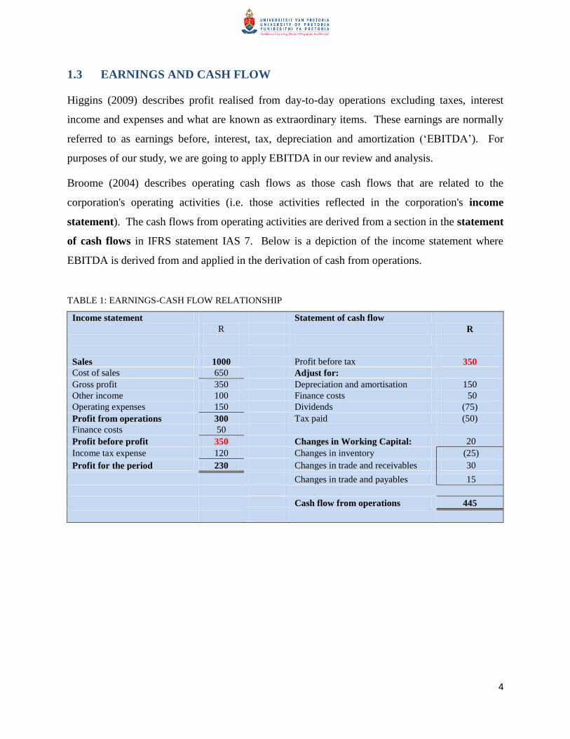
1.3 EARNINGS AND CASH FLOW
Higgins (2009) describes profit realised from day-to-day operations excluding taxes, interest
income and expenses and what are known as extraordinary items. These earnings are normally
referred to as earnings before, interest, tax, depreciation and amortization (‗EBITDA‘). For
purposes of our study, we are going to apply EBITDA in our review and analysis.
Broome (2004) describes operating cash flows as those cash flows that are related to the
corporation's operating activities (i.e. those activities reflected in the corporation's income
statement). The cash flows from operating activities are derived from a section in the statement
of cash flows in IFRS statement IAS 7. Below is a depiction of the income statement where
EBITDA is derived from and applied in the derivation of cash from operations.
TABLE 1: EARNINGS-CASH FLOW RELATIONSHIP
Income statement
Statement of cash flow
R
R
Sales
1000
Profit before tax 350
Cost of sales 650 Adjust for:
Gross profit 350 Depreciation and amortisation 150
Other income 100 Finance costs 50
Operating expenses 150 Dividends (75)
Profit from operations 300 Tax paid (50)
Finance costs 50
Profit before profit 350 Changes in Working Capital: 20
Income tax expense 120 Changes in inventory (25)
Profit for the period 230 Changes in trade and receivables 30
Changes in trade and payables 15
Cash flow from operations 445
5
IFRS further elaborates that cash flows from operating activities are primarily derived from the
principal revenue-producing activities of the entity and generally result from the activities that
generate entity‘s profit and/or losses (IFRS-IAS 7, para. 14). The point is clearly explained by
the caption above.
The amount of R350 represents the performance results in terms of profits derived by the
operations. The same amount is applied in the Statement of cash flows in determining the cash
flows from the operating activities.
IFRS has two methods to compute cash from operations; they are direct and indirect methods.
Graham and Whitfield (2010) alluded to the fact that IFRS recommends the use of the direct
method as it is easy and simpler to apply and understand.
Cash flows from operations (CFO) are arrived at by taking the EBITDA and adjust for taxes,
dividends and movements or changes in the working capital. As Finger (1994) correctly pointed
out that there is a relationship between earnings and cash flows. This relationship is formalised
by the accounting principles adopted through IFRS.
1.4 OBJECTIVES
The objectives of this research project are:
1.4.1 To investigate whether current year earnings can predict future cash flows;
1.4.2 To investigate whether current year cash flows can predict future cash flows;
1.4.3 To investigate which of the two variables; earnings or cash flows have a better
predictability of future share price;
The population of this research will therefore be drawn from the JSE listed companies as their
financial reports and annual financial statements are publicly available.
6
1.5 SCOPE OF THE RESEARCH PROBLEM
The scope of this research project is to assess which of the two variables, that is, earnings and
cash flows, will better predict the future cash flows. These two financial variables are derived
from the financial reports and annual financial statements which are prepared under the guidance
of certain accounting principles.
The scope includes the period before the adoption of the IFRS and the period after. The data is
drawn for the duration of eleven years, form 2001 to 2011, which includes the years prior and
post formal adoption post of IFRS.
In conclusion, the analysis and valuation of the research problem and providing the basis of the
research leads in further exploration what the previous authors and academics had written on this
topic before. The theoretical basis are analysed and discussed in line with that of academic
research standards.
7
Chapter 2
Literature Review
This chapter demonstrates research work that had been previously performed in other countries in
understanding the relationship between earnings and cash flows, the review of the random walk models,
further understanding the predictive capabilities of the two elements in relation to future cash flows and
future market price.
8
2. LITERATURE REVIEW
2.1 INTRODUCTION
The previous chapter introduced the background and the purpose of this research project. The
research project primarily focuses on the work performed by Kim and Ross (2005). This
particular study incorporated findings by Dechow et al. (1998) and Collins et al. (1997). This
research investigated the ability of earnings and cash flow to predict the future cash flow and
future share prices of the JSE listed companies.
The literature review demonstrated the previous work conducted by other researchers on this
topic. It revealed the historical reports that have informed the research by Kim and Kross (2005).
The theory developed was aimed at assessing earnings ability to predict future cash flows and to
review cash flows ability to predict future cash flows. Following Collins et al. (1997) study, as
re-performed by Kim and Kross (2005) the study assessed the correlation between the earnings
and book values in predicting future prices. The models were reviewed included the commonly
known model, the random walk as it was further developed by Dechow et al. (1998) in assessing
earnings ability to predict future cash flows.
2.2 EARNINGS ABILITY TO PREDICT FUTURE CASH FLOWS
This section began by reviewing the studies that were conducted by different researchers and
scholars on this topic of earnings ability to predict future cash flows which led to Kim and Kross
(2005) research report. Bowen, Burgstahler and Daley (1986) concluded that traditional
measures of cash flows, being net income (earnings) plus depreciation and amortization and
working capital from operations (as depicted on Table 1 above), are highly correlated with
earnings. These findings were in response to their research question three of their research study:
whether earnings or cash flow best predict future cash flow. A sample of 324 companies was
selected where CFO (cash from operations) being a dependent variable and an independent
variable, NIBEI (net income before extraordinary items and discontinued operations) indicated
that they strongly correlated at r = 0.587 for a one period ahead forecasts and 0.600 for a two
period ahead forecasts.
9
It was noted that WCFO (being Net Income before Depreciation and adjustments for ‗other‘
elements of NIBEI) predicts future CFOs in both in the one-period ahead forecast and two-period
ahead forecast at 0.434 and 0.425, respectively (Bowen et al., 1986). These test results indicated
that earnings had strong predictive abilities over future cash flows despite the decline.
The earlier findings by Bowen et al. (1986) were later confirmed by Charitou and Ketz (1990),
where they conceded that operating earnings (denoted as ―OPNI‖) and earnings before
depreciation (denoted as ―OPNIPD‖) and working capital from operations (―WCFO‖) correlated
strongly with each other. The results were based on a sample of 70 companies in the retail
industry and the regression tests were conducted from 1980 to 1983.
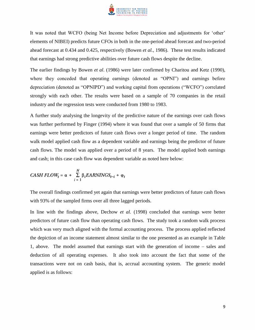
A further study analysing the longevity of the predictive nature of the earnings over cash flows
was further performed by Finger (1994) where it was found that over a sample of 50 firms that
earnings were better predictors of future cash flows over a longer period of time. The random
walk model applied cash flow as a dependent variable and earnings being the predictor of future
cash flows. The model was applied over a period of 8 years. The model applied both earnings
and cash; in this case cash flow was dependent variable as noted here below:
The overall findings confirmed yet again that earnings were better predictors of future cash flows
with 93% of the sampled firms over all three lagged periods.
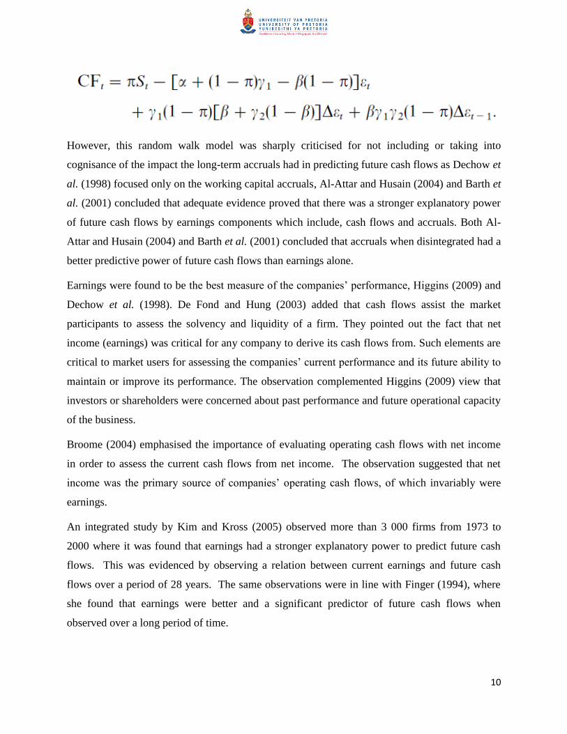
In line with the findings above, Dechow et al. (1998) concluded that earnings were better
predictors of future cash flow than operating cash flows. The study took a random walk process
which was very much aligned with the formal accounting process. The process applied reflected
the depiction of an income statement almost similar to the one presented as an example in Table
1, above. The model assumed that earnings start with the generation of income – sales and
deduction of all operating expenses. It also took into account the fact that some of the
transactions were not on cash basis, that is, accrual accounting system. The generic model
applied is as follows:
10
However, this random walk model was sharply criticised for not including or taking into
cognisance of the impact the long-term accruals had in predicting future cash flows as Dechow et
al. (1998) focused only on the working capital accruals, Al-Attar and Husain (2004) and Barth et
al. (2001) concluded that adequate evidence proved that there was a stronger explanatory power
of future cash flows by earnings components which include, cash flows and accruals. Both Al-
Attar and Husain (2004) and Barth et al. (2001) concluded that accruals when disintegrated had a
better predictive power of future cash flows than earnings alone.
Earnings were found to be the best measure of the companies‘ performance, Higgins (2009) and
Dechow et al. (1998). De Fond and Hung (2003) added that cash flows assist the market
participants to assess the solvency and liquidity of a firm. They pointed out the fact that net
income (earnings) was critical for any company to derive its cash flows from. Such elements are
critical to market users for assessing the companies‘ current performance and its future ability to
maintain or improve its performance. The observation complemented Higgins (2009) view that
investors or shareholders were concerned about past performance and future operational capacity
of the business.
Broome (2004) emphasised the importance of evaluating operating cash flows with net income
in order to assess the current cash flows from net income. The observation suggested that net
income was the primary source of companies‘ operating cash flows, of which invariably were
earnings.
An integrated study by Kim and Kross (2005) observed more than 3 000 firms from 1973 to
2000 where it was found that earnings had a stronger explanatory power to predict future cash
flows. This was evidenced by observing a relation between current earnings and future cash
flows over a period of 28 years. The same observations were in line with Finger (1994), where
she found that earnings were better and a significant predictor of future cash flows when
observed over a long period of time.
11
The contemporaneous relationship between cash flow from Operations (―CFO‖) and Earnings
provided that their correlation results to be r =0.76. This indicated a strong positive relationship.
It was noted from the same study that the predictive ability of earnings over cash flows increased
gradually over a period of time from 0.32 in the 1973 – 1982 periods to 0.54 in the 1992 – 2000
periods.
This further strengthened the earlier conclusion presented by Finger (1994) that earnings had a
higher predictive ability on future cash flows over a period of time. The argument by Al-Attar
and Hussain (2004) and Barth et al. (2001) against Dechow et al. (1998) random walk model
was stronger after the consideration of two findings by Finger (1994) and Kim and Kross (2005).
The random walk model was short term focused and did not take a long term impact of accruals
for the determination of future cash flows. To emphasise the point, Kim and Kross (2005)
records that Barth et al. (2001) in their study of the relationship between earnings components
and future cash flow predictive capabilities, they disintegrated earnings into cash flows and six
other major accrual components and run cross-sectional regressions of future operating cash
flows on the current values of the seven earnings components over the 1987-1996 period. Barth
et al. (2001) pointed out that the predictive ability of earnings over future cash flows was
enhanced when elements of earnings were disaggregated into cash flow and accruals.
A warning was raised by Allen and Cote (2005) that earnings alone were not enough to predict
future operational capacity of the firm. They further advanced the argument by pointing out that
behind earnings; there could be high levels of obsolete inventory and unpaid accounts payable,
which form part of the accruals. Although they did not discount the fact that earnings possessed
high levels of future cash flows, but they were only cautioning that at times the earnings did not
tell the full story about the companies‘ cash flow generating ability in the future.
The evidence presented above indicated that earnings had a strong predictive ability to predict
future cash flows. However, Gruca and Rego (2005) disagreed with the findings of Dechow et
al. (1998) that earnings had significant impact of the future cash flows of the company. The
study focused on the impact that customer satisfaction would have on future cash flows and
shareholder value of the companies selected as a sample where they adopted Dechow et al.
(1998) random walk model and incorporated the customer satisfaction. The following the
Variability Model as denoted below was applied:
12
The r-results showed that for one period ahead, CFt+1 and current period, CFt provided that
regression results deteriorated with r=.114 and r=.143, respectively. These findings contradicted
the earlier findings by Bowen et al. (1986); Dechow et al. (1998); Finger (1994), and Kim and
Kross (2005) that earnings had a stronger predictive ability over future cash flow over a longer
period of time. However, Gruca and Rego (2005) confirmed a stronger association between
customer satisfaction and future cash flows. It was noted that Gruca and Rego (2005) research
included smaller size public companies than that Dechow et al. (1998) sampled in their study.
A study over a period of 48 years by Givoly and Hayn (2000) found amongst that profit had
become conservative and declining. They found the reasons for such decline was not the result
of a change in the distribution of the underlying cash flows but the changes in the relationship
between cash flows and earnings, which was a result of change in accounting accruals. The
possible causes were, amongst other, the fact that manipulation of earnings by management had
been declining and therefore a decline in the application of accruals to project positive
profitability (Givoly & Hayn, 2000; Roychowdhury, 2003)
The earlier findings by Allen and Cote (2005) about the fact that earnings alone are not enough
to predict future performance is complemented by Givoly and Hayn (2000) as they further
pointed that operating cash flows presented complementary element in prediction of a company‘s
future performance. They stated that some earnings include transitory accruals that did not
persist in the future, like obsolete stock and irrecoverable debtors and mounting accounts
payables. W.T. Grant was cited as a company that had continuously reported steady growth in
earnings but filed for bankruptcy due to cash flow problems.
The accuracy of earnings was pointed out by Murdoch and Krause (2012) by arguing that
matching of expenses and income improved earnings ability to predict future cash flows. In their
argument, they further assessed the impact of inclusion of extraordinary items in the companies‘
earnings which was a warning about the principle of matching and the elimination of special
items/extraordinary items, made a significant aspect of the study.
13
In their summation they concluded that ―poor matching damages earnings‘ ability to forecast
operating cash flows, it is also likely that removing the impact special items have on earnings
will improve cash flow predictions‖ (Murdoch & Krause, 2012,p. 706)
The evidence presented above concluded that there was adequate support for earnings‘ ability to
predict future cash flows. There were some exceptions that were noted, Allen and Cote (2005)
and Gruca and Rego (2005), which were afforded as not significant adverse to the general
findings.
It should be noted that cash flows from operations did not include extraordinary items and the
cash flow prediction could be adversely skewed. The matching of expenditure and income
impacts the recognition and reversal of future accruals; as noted from Barth et al. (2001),
accruals were also significant predictors of future cash flows. Therefore the hypothesis tested is
as follows:
H1: Current earnings have the ability to predict future cash flows
2.3 CASH FLOW ABILITY TO PREDICT FUTURE CASH FLOWS
―Cash flows help market participants assess firm viability by providing information about
solvency and liquidity. Such information is potentially useful because even firms with strong
earnings ultimately rely on cash to repay debt and purchase assets‖ De Fond and Hung (2002,
p.75). The statement suggested that despite the strong earnings growth that the company reports
on, it still requires cash for its growth and for going concern purposes. It was therefore important
for financial information users and analysts to predict future cash flows by analysing the
financial information
Bowen et al. (1986) and Finger (1994) concluded that cash flow strongly predicts future cash
flows in shorter periods. Bowen et al (1986) performed a correlation of cash flows to future cash
flows over one period ahead forecasts and two period ahead forecasts the regression results
showed the r=.547 and r=.607, respectively. The results indicated a strong predictive ability of
future cash flows by cash flows in a short run. Bowen et al (1986) also concluded that cash flow
indicated very low correlations with other measures of cash flows.
14
Finger (1994) reiterated the earlier findings by Bowen et al (1986) that cash flow was slightly
superior in the short run when compared to earnings (i.e. lags 1 -2). The observation was
supported by the fact that cash flow was significant for 62% of the firms and while earnings were
54%.
Dechow et al. (1998) noted that earnings were actually current cash flows adjusted by accruals
and this observation led to the conclusion that the accruals represented all the temporary cash
flows. Table 1 above depicted the observations by Dechow et al. (1998). Broome (2004) and
Roychowdhury (2003) cautioned that at times managers do manipulate earnings through accruals
and the abuse of the accrual systems. Murdoch and Krause (2012) warned about the importance
of matching income and expenses for the accuracy of the earnings as they were capable of
predicting future cash flows. Al-Attar and Husain (2004) elaborated on matching principle as
they confirmed that expenses that generated revenue should be recognised in the financial
records in the same period.
The same principle follows the accrual system of accounting which allows the recognition of
transactions as they occurred not when cash is exchanged (IFRS, 2010). The form of accounting
principle gave rise to the accruals. Allen and Cote (2005) also warned that not all accruals
reverse into future cash flows.
Kim and Kross‘ (2005) conclusion was in line with both Bowen et al (1986) and Finger (1994)
that cash flows‘ ability to explain future cash flows was stronger in the first 2 and 3 sub-periods
in a sample of 28 year period.
De Fond and Hung (2003) argued that analysts resort to cash flow forecasts when circumstances
indicate that earnings alone are not sufficient during the periods of high earnings volatility.
Allen and Cote (2005) made a reference to Barth et al., (2001) that of the two components
between earnings, cash flow and accruals, cash flow is still stronger in predicting future
performance.
Orpurt and Zang (2007) provided that the format of the Statement of cash flows provided
different predictive capabilities of future cash flows. Graham and Whitfield (2010) alluded to
the two formats of cash flow statements, being Direct and Indirect methods. Statements of Cash
Flows adapted from Broome (2004), Table 2 – Direct Method and Table 3-Indirect Method.
15
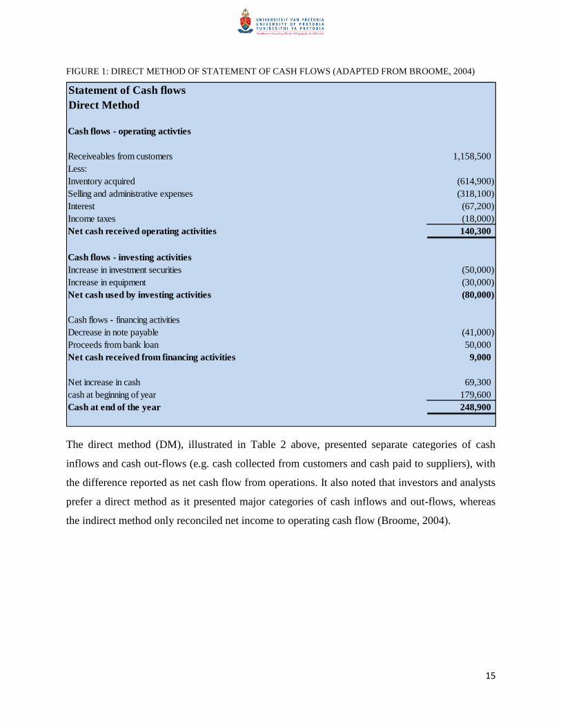
FIGURE 1: DIRECT METHOD OF STATEMENT OF CASH FLOWS (ADAPTED FROM BROOME, 2004)
The direct method (DM), illustrated in Table 2 above, presented separate categories of cash
inflows and cash out-flows (e.g. cash collected from customers and cash paid to suppliers), with
the difference reported as net cash flow from operations. It also noted that investors and analysts
prefer a direct method as it presented major categories of cash inflows and out-flows, whereas
the indirect method only reconciled net income to operating cash flow (Broome, 2004).
Statement of Cash flows
Direct Method
Cash flows - operating activties
Receiveables from customers 1,158,500
Less:
Inventory acquired (614,900)
Selling and administrative expenses (318,100)
Interest (67,200)
Income taxes (18,000)
Net cash received operating activities 140,300
Cash flows - investing activities
Increase in investment securities (50,000)
Increase in equipment (30,000)
Net cash used by investing activities (80,000)
Cash flows - financing activities
Decrease in note payable (41,000)
Proceeds from bank loan 50,000
Net cash received from financing activities 9,000
Net increase in cash 69,300
cash at beginning of year 179,600
Cash at end of the year 248,900
16
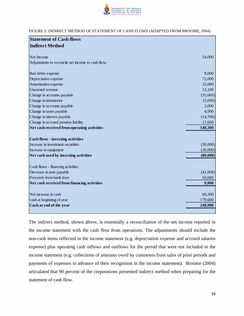
FIGURE 2: INDIRECT METHOD OF STATEMENT OF CASH FLOWS (ADAPTED FROM BROOME, 2004)
The indirect method, shown above, is essentially a reconciliation of the net income reported in
the income statement with the cash flow from operations. The adjustments should include the
non-cash items reflected in the income statement (e.g. depreciation expense and accrued salaries
expense) plus operating cash inflows and outflows for the period that were not included in the
income statement (e.g. collections of amounts owed by customers from sales of prior periods and
payments of expenses in advance of their recognition in the income statement). Broome (2004)
articulated that 90 percent of the corporations presented indirect method when preparing for the
statement of cash flow.
Statement of Cash flows
Indirect Method
Net Income 54,000
Adjustments to reconcile net income to cash flow:
Bad debts expense 8,000
Depreciation expense 72,000
Amortisation expense 25,000
Unearned revenue 12,100
Change in accounts payable (35,600)
Change in inventories (5,000)
Change in accounts payable 2,000
Change in taxes payable 4,900
Change in interest payable (14,700)
Change in accrued pension liability 17,600
Net cash received from operating activities 140,300
Cash flows - investing activities
Increase in investment securities (50,000)
Increase in equipment (30,000)
Net cash used by investing activities (80,000)
Cash flows - financing activities
Decrease in note payable (41,000)
Proceeds from bank loan 50,000
Net cash received from financing activities 9,000
Net increase in cash 69,300
cash at beginning of year 179,600
Cash at end of the year 248,900
17
The reasons for the choice is simplicity as previously stated by Graham and Whitfield (2010),
however reconciliation of net income and accruals provided cash flow from operations (Broome,
2004). An example of such reconciliation is presented in Figure 1 above.
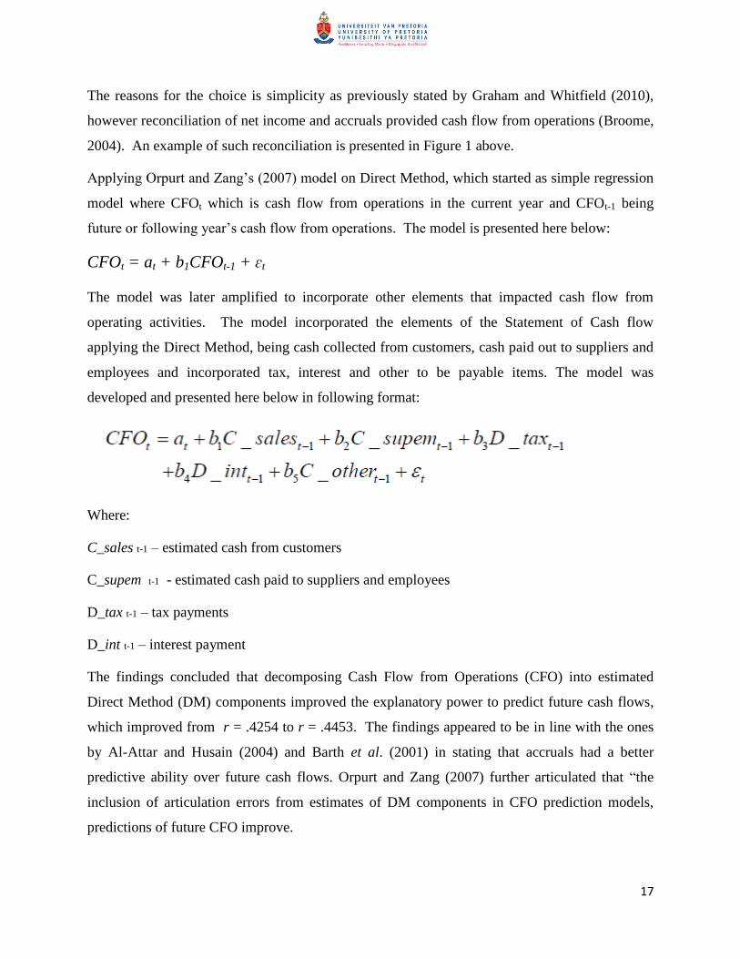
Applying Orpurt and Zang‘s (2007) model on Direct Method, which started as simple regression
model where CFOt which is cash flow from operations in the current year and CFOt-1 being
future or following year‘s cash flow from operations. The model is presented here below:
CFOt = at + b1CFOt-1 + ɛt
The model was later amplified to incorporate other elements that impacted cash flow from
operating activities. The model incorporated the elements of the Statement of Cash flow
applying the Direct Method, being cash collected from customers, cash paid out to suppliers and
employees and incorporated tax, interest and other to be payable items. The model was
developed and presented here below in following format:
Where:
C_sales t-1 – estimated cash from customers
C_supem t-1 - estimated cash paid to suppliers and employees
D_tax t-1 – tax payments
D_int t-1 – interest payment
The findings concluded that decomposing Cash Flow from Operations (CFO) into estimated
Direct Method (DM) components improved the explanatory power to predict future cash flows,
which improved from r = .4254 to r = .4453. The findings appeared to be in line with the ones
by Al-Attar and Husain (2004) and Barth et al. (2001) in stating that accruals had a better
predictive ability over future cash flows. Orpurt and Zang (2007) further articulated that ―the
inclusion of articulation errors from estimates of DM components in CFO prediction models,
predictions of future CFO improve.
18
The improvement occurs whether income statement and either IM statement of cash flows data
or balance sheet data are used to estimate DM components‖ (p. 30). It was evident that future
cash flow predictions would not be possible without taking into account the accruals.
In conclusion, cash flows possessed stronger predictive ability over future cash flows in the short
run. In order to achieve accurate future cash flows, accurate computation and measurement of
earnings and accruals are imperative.
H2: Current year’s cash flows from operations have the ability to predict future cash
flows
2.4 EARNINGS AND CASH FLOWS AS PREDICTORS OF FUTURE SHARE
PRICE
Charitou and Ketz (1990) argued that there was some consensus that share prices were related to
the future cash flows of the firms and reiterated that there remains some controversy and
confusion to the ex post earnings and cash flow measures in signalling share prices. The
argument presented required a further exploration as to the significance of earnings and cash
flow in the prediction of future share price.
2.4.1 EARNINGS AS THE PREDICTOR OF FUTURE SHARE PRICE
Bandyopadhyay, Chen, Huang and Jha (2010) reiterated the findings by Collins et al, (1997)
where earnings were found to be no longer useful in explaining contemporaneous relationship
with share prices due to the declining relationship over time.
The conclusion by Collins et al. (1997) was a result of the incremental regression relation of
earnings for explaining share prices over book values declined from 30 percent during 1953 –
1962 whereas the findings of Kim and Kross (2005) showed a further deterioration to 5.7 percent
for the period from 1983 to 1993.
Earnings on the other hand indicated high predictive power on the future cash flows (Kim &
Kross, 2005). Bandyopadhyay et al. (2010) argued that share price represented the present value
of future cash flows and a logical thing that could have occurred was for earnings to indicate
contemporaneous relationship with the share prices. Bandyopadhyay et al (2010) investigated
further the possible causes of the decline of the contemporaneous relationship between earnings
and share price over time where they concluded that the conservative accounting principles that
19
had been implemented over a period of time had resulted in earnings being conservative as a
result; they became irrelevant in predicting future share prices. The findings raised more
questions when referred to Collins et al. (1997) findings where over a research over a period of
41 years was conducted ranging from 1953 to 1993 and the model included the price which was
expressed as a function of both earnings and book value of equity. The explanatory power was
further decomposed into three components being: (1) the incremental power of earnings; (2) the
incremental power of book values, and (3) the explanatory power common to both earnings and
book values. The following models were applied and regressed separately as follows:
Pit = α0t +α1tEit+α2tBVit+ɛit [7]
Pit = β0t + β1tEit +ɛit [8]
And
Pit = χ0t + χ1tBVit + ɛit [9]
The BV was the book value per share of firm I at year-end t. P was the price of a share of firm I
three months after year-end t. E was the earnings per share of firm I for year t.
Earnings and book values positively correlated with each other. However, the cross-sectional
regression of price to earnings deteriorated from r = 0.299 in the years from 1953 to 1962; in the
period from 1983 to 1993 the results indicated r = 0.070. The regressions correlation between
the price and book value increased over the period of time. The results indicated r = 0.004 (1953
to 1962) to r = 0.186 (1983 to 1993).
Bandyopadhyay‘s et al. (2010) conclusion could be further explored given the era when their
data was drawn is different from Collins et al. (1997) and Kim and Kross (2005) but the results
were the same. The latter (2005) conducted similar study in a different era but arrived at the
same conclusion to that of Collins et al (1997), given the fact that the new accounting principles
had been introduced gradually over a period of time (Reidl, 2010). Conservatism in accounting
principles had produced high quality earnings (Penman & Zhang, 2002). Their findings further
concluded that conservatism produced lower earnings but higher quality. High quality of
earnings defined as: ―reported earnings, before extraordinary items that are readily identified on
20
the income statement, is of good quality if it is a good indicator of future earnings‖ (Penman &
Zhang, 2002, p.237).
Hecht and Vuolteenaho (2006) concluded that there was a low correlation between stock returns
and earnings. These findings suggested that earnings had little impact on the future share price.
Bali, Demirtas and Tehranian (2008) argued that aggregated earnings yield provide little or no
forecasting power for aggregate share returns. They also found that earnings positively
correlated with business conditions and negatively correlated with expected returns.
Billings and Morton (2001) found that their investigation of the book-to-market‘s ability to
predict future earnings was low. The tests conducted included short term which was one year
ahead forecast (t+1), two-year forecast (t+2) and long term (lgt). The correlation results
indicated r = 0.271 (short-term), r = 0.270 (two year ahead forecast) and r=0.255 in the long
term. The results indicated a very low correlation between the book-to-market and future
earnings. The reverse had proven to be the case given the findings that had been cited above that
the relationship between share price and earnings is low.
In contrary to what had been established above, Penman and Zhang (2002) concluded that
quality of earnings scored incrementally in predicting future stock returns, before transaction
costs, over the 1976 to 1995 of 38 450 sample of NYSE listed firms. However, this was
concluded after controlling measures commonly estimated as risk proxies, and after controlling
for growth in net operating assets (investments) and for accruals. A similar observation was
conveyed by Ryan and Zarowin (2003) that earnings had a weaker association with current price
changes and a stronger association with lagged price changes over a period of time.
These two contrasting views presented a motivation for further investigations as to whether
earnings had the ability to predict future share prices. Therefore, the hypothesis test is concluded
to be:
H3: Current earnings have the ability to predict future share price
21
2.4.2 CASH FLOW AS THE PREDICTOR OF FUTURE SHARE PRICE
Dontoh, Radhakrishnan and Ronen (2007) in their comparison of share price and accounting data
found that the association had been declining. Accounting data in this case was represented by
cash flow from operations (CFO). The poor association was attributed to the possible ―noises‖ in
the market which had landed to such a low relations. DeFond and Huang (2003) took a view that
cash flow forecasts depended on the accounting, operating and financing characteristics that
determine the extent of the usefulness of cash flow and earnings and firm future operating
capabilities. Therefore, it was concluded that accounting data, cash flow from operations in
particular, are important in determining the future viability of the firm which impact the future
share price.
Platt, Demirkan and Platt (2010) questioned whether the discounted future cash flows resulted
into company value. It was noted that to predict future value of the company, future estimated
cash flows should have been sorted. Kaplan and Rubeck (1994) argued that there was no
evidence that discounted cash flows provide a reliable estimate of market value or share prices.
There were other factors that contributed to the company value. Gruca and Rego (2005) inferred
that customer satisfaction resulted in shareholder value being increased and consequently
improved cash flows. It could be argued whether shareholder value and firm value were the
same. Charitou and Ketz (1990) noted that the share price was determined by the cash flows of
the firm discounted by a discounting factor which considers the time value of money and
adjusted for riskiness in the market. And this could be achieved where estimated future cash
flows were used in estimating company value by discounting estimated future cash flows. This
computation is performed by estimating free cash flow (FCF) which is normally EBITDA
adjusted by accruals (Platt et al., 2010).
Hecht and Vuolteenaho (2006) found that correlations between cash flow proxies with one
period expected returns, cash-flow news and expected returns news explained expected returns
well. Cohen, Gompers and Vuolteenaho (2002) found that cash-flow news were a single
measure of the change in the permanent component of the share price.
22
From the evidence presented by the scholars above, it could be concluded that investors acquire
shares with a view of future returns and future cash flows anticipation, therefore any news that
indicated future cash flows could result in shares being acquired. But this did not provide
conclusive evidence that cash flow had the ability to predict future share prices.
Choy and Sais (2012) argued that strong financial information had some predictive ability over
future share price. They argued that investors would acquire shares of companies with strong
financial condition as they were perceived as undervalued. A strong financial condition would
naturally incorporate publicly available data which include the statement of cash flow. Cohen
and Kudryadstev (2012) found that investment in shares was influenced by expectations, past
experience in the capital market, and knowledge about the past performance of selected market
indices. Again, it could be argued that past cash flow generation propensity could positively
impact investors‘ decision to acquire the shares. It was also considered that from a generally
known economics phenomenon that share prices are also influenced amongst other things, by the
demand and supply.
Kim and Kross (2005) found that the contemporaneous relationship between price and cash
flows showed a declining trend. The explanatory power of cash flow over price for the period,
1973 to 1982 recorded at 10.8%, period 1983 – 1991 indicated 9.6% and the period between
1992 and 2000 showed a further decline to 7.9%. A similar decline was noted between price and
accruals where the correlation declined from 9.1% to 6.0 to the lowest of 5.6% within the same
period as above.
The findings above strongly indicated that cash flow had no direct ability to predict future share
prices. Cash flow was embedded in the corporate earnings and therefore investors and analysts
relied heavily on reported performance (Banker et al., 2009).
The arguments advanced by Orpurt and Zang (2007) the DM type of Statement of Cash Flow
had a more predictive power of future cash flows and earnings; it also provided that accruals on
the face of it did not provide same predictive ability for future share prices.
23
The company valuation techniques like the Free Cash Flow method, which relied on estimated
future cash flows could not provide evidence that they were able to predict future share prices
due to the so called noises and riskiness in the market, changes in growth and changes in
persistence of earnings (Charitou & Ketz, 1990; Kaplan & Rubeck 1994; Kim & Kross, 2005
and Platt et al. 2010)
H4: Current year’s cash flows have the ability to predict future share prices
24
2.5 THE MODELS
2.5.1 BACKGROUND
In chapter 1 the key objectives of the research project were presented to be:
The assessment of the predictive ability of current year earnings over future cash flows of
JSE listed companies in the short and long term;
The assessment of the predictive ability of current year cash flows over future cash flows
of the JSE listed companies in the short and long term; and
The assessment which of the two variables, earnings or cash flows are better predictor of
future market share price both in short and long term
Previous researchers, scholars and writers on this similar research projects had applied models to
assess the predictive abilities of one variable over the other. This section of this chapter
discussed and assessed different types of models that assisted in evaluating the information and
presented the appropriate outcomes.
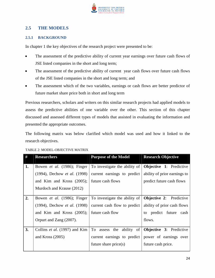
The following matrix was below clarified which model was used and how it linked to the
research objectives.
TABLE 2: MODEL-OBJECTIVE MATRIX
# Researchers Purpose of the Model Research Objective
1. Bowen et al. (1986); Finger
(1994), Dechow et al. (1998)
and Kim and Kross (2005);
Murdoch and Krause (2012)
To investigate the ability of
current earnings to predict
future cash flows
Objective 1: Predictive
ability of prior earnings to
predict future cash flows
2. Bowen et al. (1986); Finger
(1994), Dechow et al. (1998)
and Kim and Kross (2005);
Orpurt and Zang (2007).
To investigate the ability of
current cash flow to predict
future cash flow
Objective 2: Predictive
ability of prior cash flows
to predict future cash
flows.
3. Collins et al. (1997) and Kim
and Kross (2005)
To assess the ability of
current earnings to predict
future share price(s)
Objective 3: Predictive
power of earnings over
future cash price.
25
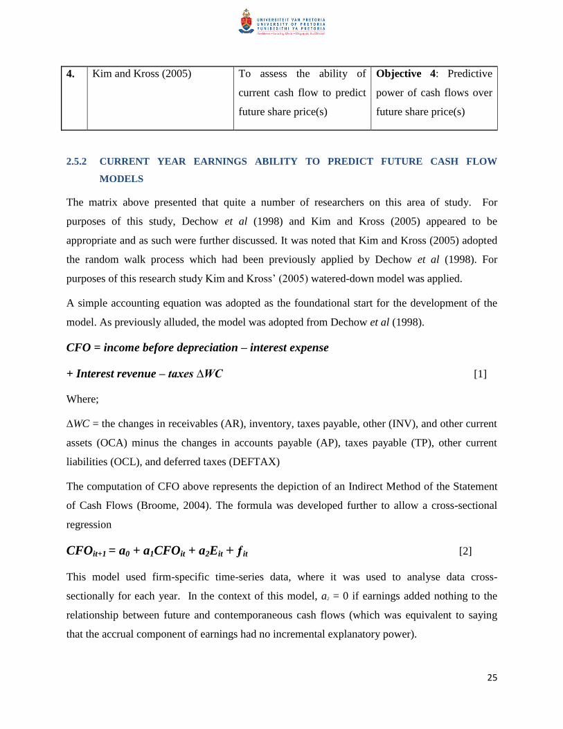
4. Kim and Kross (2005) To assess the ability of
current cash flow to predict
future share price(s)
Objective 4: Predictive
power of cash flows over
future share price(s)
2.5.2 CURRENT YEAR EARNINGS ABILITY TO PREDICT FUTURE CASH FLOW
MODELS
The matrix above presented that quite a number of researchers on this area of study. For
purposes of this study, Dechow et al (1998) and Kim and Kross (2005) appeared to be
appropriate and as such were further discussed. It was noted that Kim and Kross (2005) adopted
the random walk process which had been previously applied by Dechow et al (1998). For
purposes of this research study Kim and Kross‘ (2005) watered-down model was applied.
A simple accounting equation was adopted as the foundational start for the development of the
model. As previously alluded, the model was adopted from Dechow et al (1998).
CFO = income before depreciation – interest expense
+ Interest revenue – taxes ∆WC [1]
Where;
∆WC = the changes in receivables (AR), inventory, taxes payable, other (INV), and other current
assets (OCA) minus the changes in accounts payable (AP), taxes payable (TP), other current
liabilities (OCL), and deferred taxes (DEFTAX)
The computation of CFO above represents the depiction of an Indirect Method of the Statement
of Cash Flows (Broome, 2004). The formula was developed further to allow a cross-sectional
regression
CFOit+1 = a0 + a1CFOit + a2Eit + ƒit [2]
This model used firm-specific time-series data, where it was used to analyse data cross-
sectionally for each year. In the context of this model, a2 = 0 if earnings added nothing to the
relationship between future and contemporaneous cash flows (which was equivalent to saying
that the accrual component of earnings had no incremental explanatory power).
26
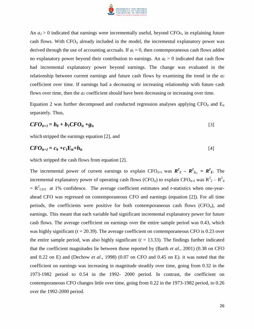
An a2 > 0 indicated that earnings were incrementally useful, beyond CFOit, in explaining future
cash flows. With CFOit already included in the model, the incremental explanatory power was
derived through the use of accounting accruals. If al = 0, then contemporaneous cash flows added
no explanatory power beyond their contribution to earnings. An al > 0 indicated that cash flow
had incremental explanatory power beyond earnings. The change was evaluated in the
relationship between current earnings and future cash flows by examining the trend in the a2
coefficient over time. If earnings had a decreasing or increasing relationship with future cash
flows over time, then the a2 coefficient should have been decreasing or increasing over time.
Equation 2 was further decomposed and conducted regression analyses applying CFOit and Eit
separately. Thus,
CFOit+1 = b0 + b1CFOit +git [3]
which stripped the earnings equation [2], and
CFOit+1 = c0 +c1Eit+hit [4]
which stripped the cash flows from equation [2].
The incremental power of current earnings to explain CFOit+l was R2
2 – R2
3_ = R2
E. The
incremental explanatory power of operating cash flows (CFOit) to explain CFOit+l was R22 – R
24
= R2
CFO at 1% confidence. The average coefficient estimates and t-statistics when one-year-
ahead CFO was regressed on contemporaneous CFO and earnings (equation [2]). For all time
periods, the coefficients were positive for both contemporaneous cash flows (CFOit), and
earnings. This meant that each variable had significant incremental explanatory power for future
cash flows. The average coefficient on earnings over the entire sample period was 0.43, which
was highly significant (t = 20.39). The average coefficient on contemporaneous CFO is 0.23 over
the entire sample period, was also highly significant (t = 13.33). The findings further indicated
that the coefficient magnitudes lie between those reported by (Barth et al., 2001) (0.38 on CFO
and 0.22 on E) and (Dechow et al., 1998) (0.07 on CFO and 0.45 on E). it was noted that the
coefficient on earnings was increasing in magnitude steadily over time, going from 0.32 in the
1973-1982 period to 0.54 in the 1992- 2000 period. In contrast, the coefficient on
contemporaneous CFO changes little over time, going from 0.22 in the 1973-1982 period, to 0.26
over the 1992-2000 period.
27
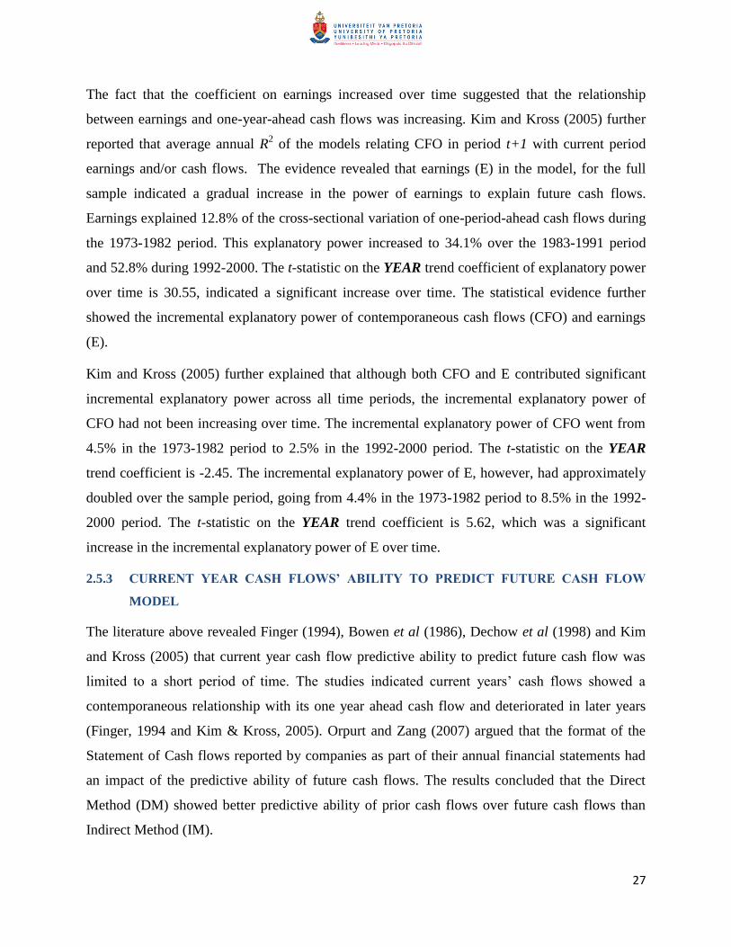
The fact that the coefficient on earnings increased over time suggested that the relationship
between earnings and one-year-ahead cash flows was increasing. Kim and Kross (2005) further
reported that average annual R2 of the models relating CFO in period t+1 with current period
earnings and/or cash flows. The evidence revealed that earnings (E) in the model, for the full
sample indicated a gradual increase in the power of earnings to explain future cash flows.
Earnings explained 12.8% of the cross-sectional variation of one-period-ahead cash flows during
the 1973-1982 period. This explanatory power increased to 34.1% over the 1983-1991 period
and 52.8% during 1992-2000. The t-statistic on the YEAR trend coefficient of explanatory power
over time is 30.55, indicated a significant increase over time. The statistical evidence further
showed the incremental explanatory power of contemporaneous cash flows (CFO) and earnings
(E).
Kim and Kross (2005) further explained that although both CFO and E contributed significant
incremental explanatory power across all time periods, the incremental explanatory power of
CFO had not been increasing over time. The incremental explanatory power of CFO went from
4.5% in the 1973-1982 period to 2.5% in the 1992-2000 period. The t-statistic on the YEAR
trend coefficient is -2.45. The incremental explanatory power of E, however, had approximately
doubled over the sample period, going from 4.4% in the 1973-1982 period to 8.5% in the 1992-
2000 period. The t-statistic on the YEAR trend coefficient is 5.62, which was a significant
increase in the incremental explanatory power of E over time.
2.5.3 CURRENT YEAR CASH FLOWS’ ABILITY TO PREDICT FUTURE CASH FLOW
MODEL
The literature above revealed Finger (1994), Bowen et al (1986), Dechow et al (1998) and Kim
and Kross (2005) that current year cash flow predictive ability to predict future cash flow was
limited to a short period of time. The studies indicated current years‘ cash flows showed a
contemporaneous relationship with its one year ahead cash flow and deteriorated in later years
(Finger, 1994 and Kim & Kross, 2005). Orpurt and Zang (2007) argued that the format of the
Statement of Cash flows reported by companies as part of their annual financial statements had
an impact of the predictive ability of future cash flows. The results concluded that the Direct
Method (DM) showed better predictive ability of prior cash flows over future cash flows than
Indirect Method (IM).
28
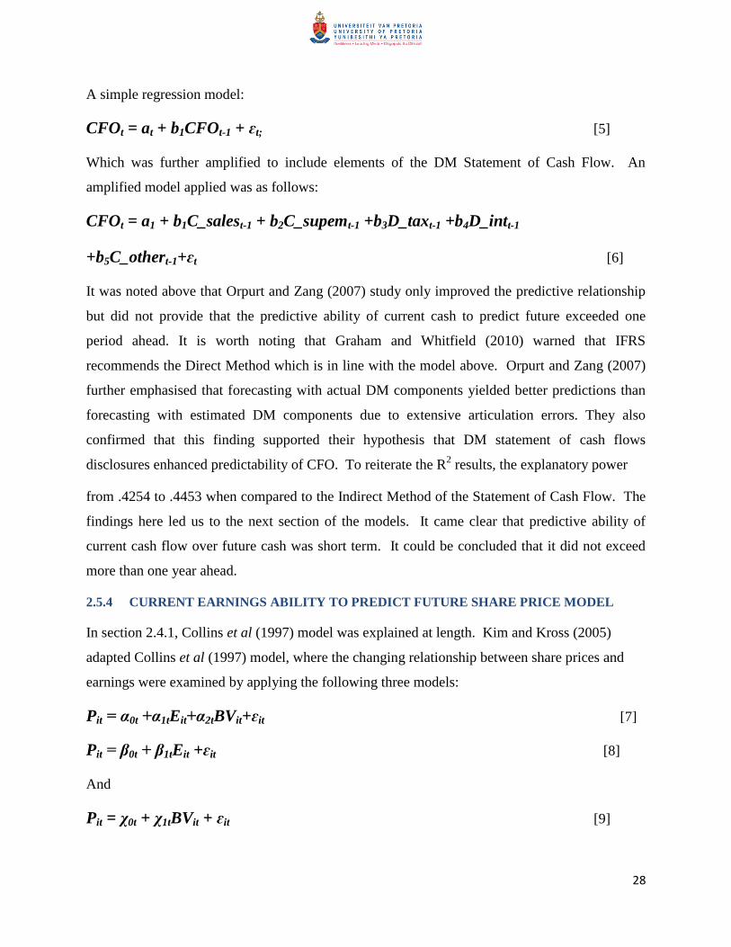
A simple regression model:
CFOt = at + b1CFOt-1 + ɛt; [5]
Which was further amplified to include elements of the DM Statement of Cash Flow. An
amplified model applied was as follows:
CFOt = a1 + b1C_salest-1 + b2C_supemt-1 +b3D_taxt-1 +b4D_intt-1
+b5C_othert-1+ɛt [6]
It was noted above that Orpurt and Zang (2007) study only improved the predictive relationship
but did not provide that the predictive ability of current cash to predict future exceeded one
period ahead. It is worth noting that Graham and Whitfield (2010) warned that IFRS
recommends the Direct Method which is in line with the model above. Orpurt and Zang (2007)
further emphasised that forecasting with actual DM components yielded better predictions than
forecasting with estimated DM components due to extensive articulation errors. They also
confirmed that this finding supported their hypothesis that DM statement of cash flows
disclosures enhanced predictability of CFO. To reiterate the R2 results, the explanatory power
from .4254 to .4453 when compared to the Indirect Method of the Statement of Cash Flow. The
findings here led us to the next section of the models. It came clear that predictive ability of
current cash flow over future cash was short term. It could be concluded that it did not exceed
more than one year ahead.
2.5.4 CURRENT EARNINGS ABILITY TO PREDICT FUTURE SHARE PRICE MODEL
In section 2.4.1, Collins et al (1997) model was explained at length. Kim and Kross (2005)
adapted Collins et al (1997) model, where the changing relationship between share prices and
earnings were examined by applying the following three models:
Pit = α0t +α1tEit+α2tBVit+ɛit [7]
Pit = β0t + β1tEit +ɛit [8]
And
Pit = χ0t + χ1tBVit + ɛit [9]
29
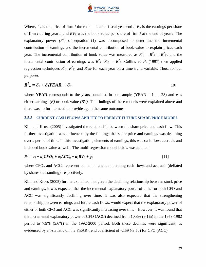
Where, Pit is the price of firm i three months after fiscal year-end t, Eit is the earnings per share
of firm i during year t, and BVit was the book value per share of firm i at the end of year t. The
explanatory power (R2) of equation (1) was decomposed to determine the incremental
contribution of earnings and the incremental contribution of book value to explain prices each
year. The incremental contribution of book value was measured as R2
1 – R22 = R
2BV and the
incremental contribution of earnings was R2
1- R2
3 = R2
E. Collins et al. (1997) then applied
regression techniques R2
1, R2E, and R
2BV for each year on a time trend variable. Thus, for our
purposes
R2
vt = δ0 + δ1YEARt + δit [10]
where YEAR corresponds to the years contained in our sample (YEAR = 1,...., 28) and v is
either earnings (E) or book value (BV). The findings of these models were explained above and
there was no further need to provide again the same outcomes.
2.5.5 CURRENT CASH FLOWS ABILITY TO PREDICT FUTURE SHARE PRICE MODEL
Kim and Kross (2005) investigated the relationship between the share price and cash flow. This
further investigation was influenced by the findings that share price and earnings was declining
over a period of time. In this investigation, elements of earnings, this was cash flow, accruals and
included book value as well. The multi-regression model below was applied:
Pit = a0 + a1CFOit + a2ACCit + a3BVit + git [11]
where CFOit and ACCit represent contemporaneous operating cash flows and accruals (deflated
by shares outstanding), respectively.
Kim and Kross (2005) further explained that given the declining relationship between stock price
and earnings, it was expected that the incremental explanatory power of either or both CFO and
ACC was significantly declining over time. It was also expected that the strengthening
relationship between earnings and future cash flows, would expect that the explanatory power of
either or both CFO and ACC was significantly increasing over time. However, it was found that
the incremental explanatory power of CFO (ACC) declined from 10.8% (9.1%) in the 1973-1982
period to 7.9% (5.6%) in the 1992-2000 period. Both these declines were significant, as
evidenced by a t-statistic on the YEAR trend coefficient of -2.59 (-3.50) for CFO (ACC).
30
This indicated that the reduction in the relation between prices and earnings over time is due to a
declining explanatory power of both cash flows (CFO) and accruals (ACC).
The models above were applied (some were adjusted accordingly in Chapter 4.
2.6 CONCLUSION
In this chapter, literature review and previous research reports were explored. It was concluded
that current earnings had a high predictive ability on future cash flows (Dechow et al., 1998;
Finger, 1994; Kim & Kross, 2005; Murdoch & Krause, 2012). Further studies also provided
information about cash flows‘ ability to predict future cash flow. Findings obtained from
previous scholars was that cash flow was only able to predict future cash flow only in the short
term (Barth et al., 2001; Bowen et al., 1986; Dechow et al., 1998; Finger, 1994; Kim & Kross,
2005; Al-Attar & Hussain 2004) provided that the disintegration of earnings components, that is,
accruals and cash flows predicted future cash flows better. Orpurt and Zang (2007) concluded
that the direct method of the Statement of Cash flows provided better predictive ability of cash
flow. Collins et al (1997) and Kim and Kross (2005) provided that the relationship between
earning and prices decline over a period of time whereas, the relationship between future price
and book value improved. The relationship between the cash flows and future price also
followed the earnings trend, showed their inability to predict future share price, (Kim & Kross,
2005).
The next chapter provided the hypotheses that were tested applying data collected from the JSE
for the period between 2001 and 2011. The introduction stated that JSE listed companies
formally adopted IFRS. Therefore, the abilities of earnings and cash flows to predict future cash
flows and prices before and after 1 January 2005 were tested.

31
Chapter 3
Research Hypothesis
This chapter presents the research problem and the associated research hypotheses
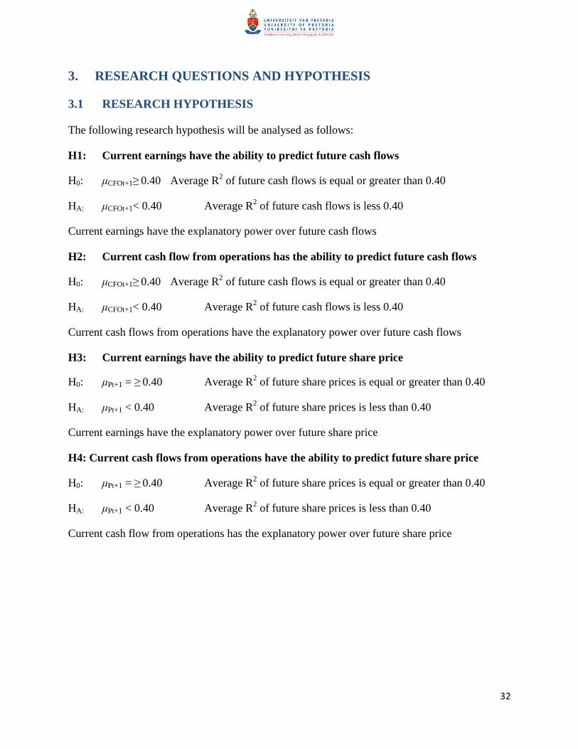
32
3. RESEARCH QUESTIONS AND HYPOTHESIS
3.1 RESEARCH HYPOTHESIS
The following research hypothesis will be analysed as follows:
H1: Current earnings have the ability to predict future cash flows
H0: μCFOt+1≥ 0.40 Average R2 of future cash flows is equal or greater than 0.40
HA: μCFOt+1< 0.40 Average R2 of future cash flows is less 0.40
Current earnings have the explanatory power over future cash flows
H2: Current cash flow from operations has the ability to predict future cash flows
H0: μCFOt+1≥ 0.40 Average R2 of future cash flows is equal or greater than 0.40
HA: μCFOt+1< 0.40 Average R2 of future cash flows is less 0.40
Current cash flows from operations have the explanatory power over future cash flows
H3: Current earnings have the ability to predict future share price
H0: μPt+1 = ≥ 0.40 Average R2 of future share prices is equal or greater than 0.40
HA: μPt+1 < 0.40 Average R2 of future share prices is less than 0.40
Current earnings have the explanatory power over future share price
H4: Current cash flows from operations have the ability to predict future share price
H0: μPt+1 = ≥ 0.40 Average R2 of future share prices is equal or greater than 0.40
HA: μPt+1 < 0.40 Average R2 of future share prices is less than 0.40
Current cash flow from operations has the explanatory power over future share price
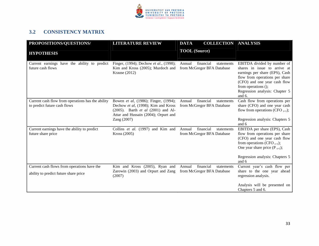
33
3.2 CONSISTENCY MATRIX
PROPOSITIONS/QUESTIONS/
HYPOTHESIS
LITERATURE REVIEW DATA COLLECTION
TOOL (Source)
ANALYSIS
Current earnings have the ability to predict
future cash flows
Finger, (1994); Dechow et al., (1998);
Kim and Kross (2005); Murdoch and
Krause (2012)
Annual financial statements
from McGregor BFA Database
EBITDA divided by number of
shares in issue to arrive at
earnings per share (EPS), Cash
flow from operations per share
(CFO) and one year cash flow
from operations ();
Regression analysis: Chapter 5
and 6.
Current cash flow from operations has the ability
to predict future cash flows
Bowen et al, (1986); Finger, (1994);
Dechow et al, (1998); Kim and Kross
(2005). Barth et al (2001) and Al-
Attar and Hussain (2004); Orpurt and
Zang (2007)
Annual financial statements
from McGregor BFA Database
Cash flow from operations per
share (CFO) and one year cash
flow from operations (CFO t+1);
Regression analysis: Chapters 5
and 6
Current earnings have the ability to predict
future share price
Collins et al. (1997) and Kim and
Kross (2005)
Annual financial statements
from McGregor BFA Database
EBITDA per share (EPS), Cash
flow from operations per share
(CFO) and one year cash flow
from operations (CFO t+1);
One year share price (P t+1);
Regression analysis: Chapters 5
and 6
Current cash flows from operations have the
ability to predict future share price
Kim and Kross (2005), Ryan and
Zarowin (2003) and Orpurt and Zang
(2007)
Annual financial statements
from McGregor BFA Database
Current year‘s cash flow per
share to the one year ahead
regression analysis.
Analysis will be presented on
Chapters 5 and 6.

34
Chapter 4
Research Methodology
This chapter presents the research method to be followed for this study and discusses the population,
sample, data collection process, data analysis and foreseen research limitation.
35
4. RESEARCH METHODOLOGY
The purpose of this study was to test the ability of current earnings and current cash from
operations to predict future cash flow and future share prices. The survey was conducted based
on the financial data of JSE listed companies. The financial information was drawn from
McGregor BFA database for the period from January 2001 to December 2011.
The study adopted quite a number of models that were applied to investigate the predictive
abilities of earnings and cash flow over the future cash flows and share prices. Chapter 2 section
2.5 presented a number of models that were applied to verify the information and some were
modified due limitations associated with gathering of information from the database.
4.1 RATIONALE OF THE RESEARCH METHOD
Again, the objective of this study was to find evidence that will explain the ability of current
earnings and current operating cash flows would have on future cash flows and future share
prices. The purpose of explanatory studies is to establish the relationship between or among
different variables (Saunders, Lewis and Thornhill , 2009). Such studies assist in diagnosing the
dimensions of a problem so that successive research projects can be undertaken successfully
Zikmund (2003).
4.2 UNIT OF ANALYSIS
Units of analysis applied were as follows:
EPS: which is determined by the dividing the EBITDA by the number of weighted
shares issued;
CFO: calculated by dividing Cash flow from operations by the number of weighted
shares issued;
P: share price as quoted on the JSE at the end of each financial year of each
company;
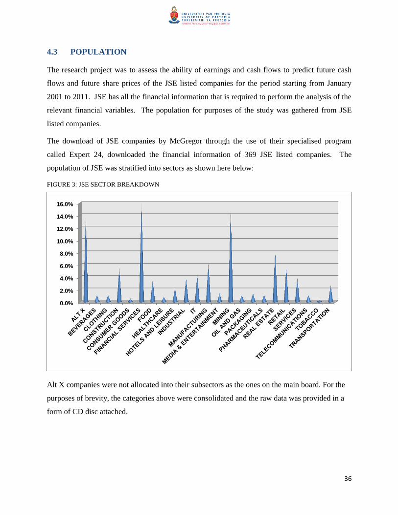
36
4.3 POPULATION
The research project was to assess the ability of earnings and cash flows to predict future cash
flows and future share prices of the JSE listed companies for the period starting from January
2001 to 2011. JSE has all the financial information that is required to perform the analysis of the
relevant financial variables. The population for purposes of the study was gathered from JSE
listed companies.
The download of JSE companies by McGregor through the use of their specialised program
called Expert 24, downloaded the financial information of 369 JSE listed companies. The
population of JSE was stratified into sectors as shown here below:
FIGURE 3: JSE SECTOR BREAKDOWN
Alt X companies were not allocated into their subsectors as the ones on the main board. For the
purposes of brevity, the categories above were consolidated and the raw data was provided in a
form of CD disc attached.
0.0%
2.0%
4.0%
6.0%
8.0%
10.0%
12.0%
14.0%
16.0%
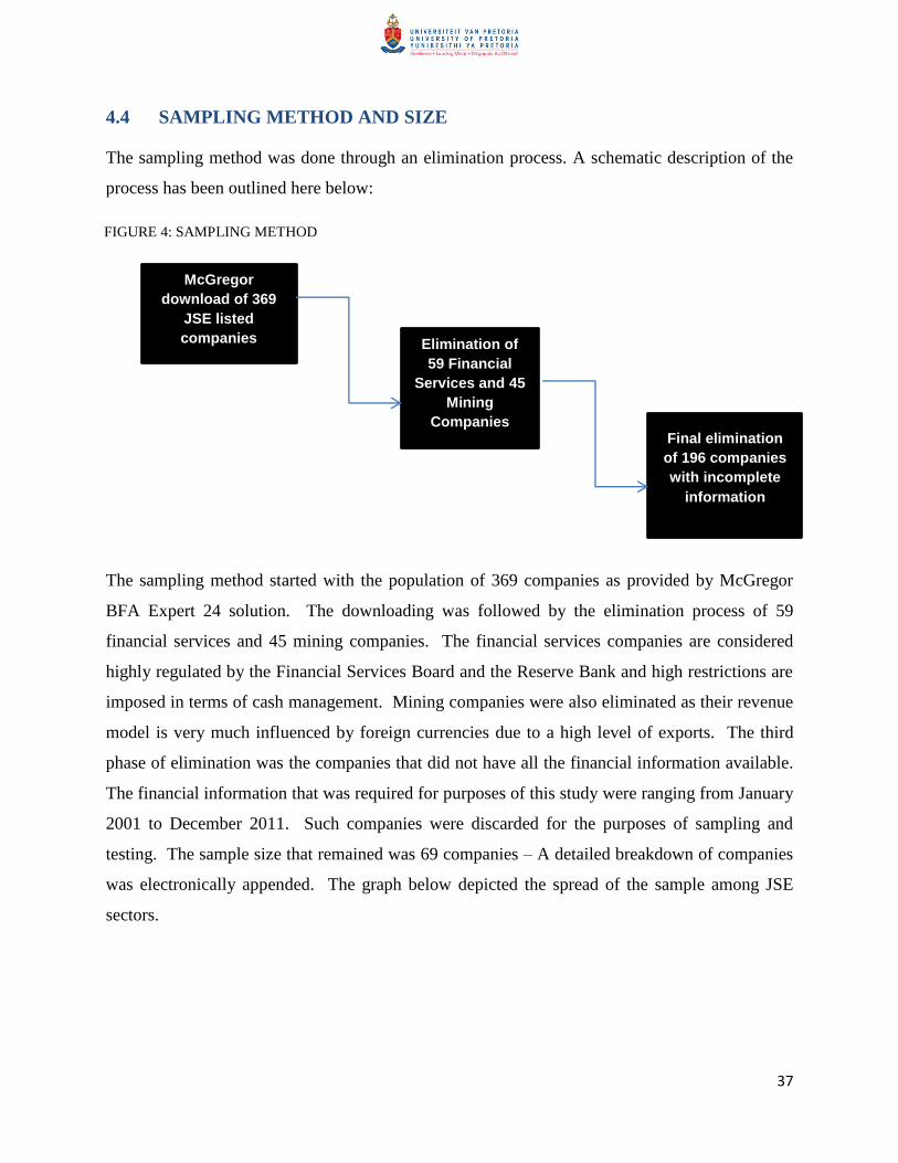
37
4.4 SAMPLING METHOD AND SIZE
The sampling method was done through an elimination process. A schematic description of the
process has been outlined here below:
The sampling method started with the population of 369 companies as provided by McGregor
BFA Expert 24 solution. The downloading was followed by the elimination process of 59
financial services and 45 mining companies. The financial services companies are considered
highly regulated by the Financial Services Board and the Reserve Bank and high restrictions are
imposed in terms of cash management. Mining companies were also eliminated as their revenue
model is very much influenced by foreign currencies due to a high level of exports. The third
phase of elimination was the companies that did not have all the financial information available.
The financial information that was required for purposes of this study were ranging from January
2001 to December 2011. Such companies were discarded for the purposes of sampling and
testing. The sample size that remained was 69 companies – A detailed breakdown of companies
was electronically appended. The graph below depicted the spread of the sample among JSE
sectors.
McGregor
download of 369
JSE listed
companies Elimination of
59 Financial
Services and 45
Mining
Companies Final elimination
of 196 companies
with incomplete
information
FIGURE 4: SAMPLING METHOD
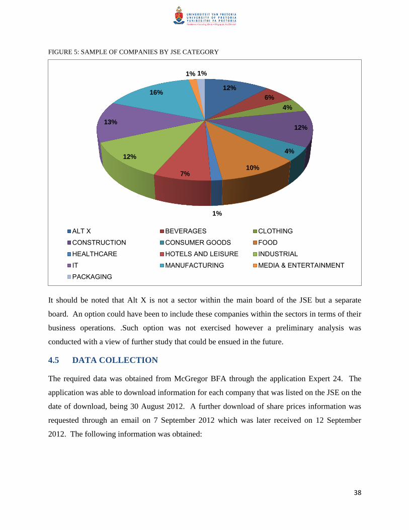
38
FIGURE 5: SAMPLE OF COMPANIES BY JSE CATEGORY
It should be noted that Alt X is not a sector within the main board of the JSE but a separate
board. An option could have been to include these companies within the sectors in terms of their
business operations. .Such option was not exercised however a preliminary analysis was
conducted with a view of further study that could be ensued in the future.
4.5 DATA COLLECTION
The required data was obtained from McGregor BFA through the application Expert 24. The
application was able to download information for each company that was listed on the JSE on the
date of download, being 30 August 2012. A further download of share prices information was
requested through an email on 7 September 2012 which was later received on 12 September
2012. The following information was obtained:
12%
6%
4%
12%
4%
10%
1%
7%
12%
13%
16%
1% 1%
ALT X BEVERAGES CLOTHING
CONSTRUCTION CONSUMER GOODS FOOD
HEALTHCARE HOTELS AND LEISURE INDUSTRIAL
IT MANUFACTURING MEDIA & ENTERTAINMENT
PACKAGING
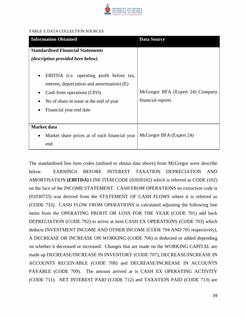
39
TABLE 3; DATA COLLECTION SOURCES
Information Obtained Data Source
Standardised Financial Statements
(description provided here below)
EBITDA (i.e. operating profit before tax,
interest, depreciation and amortisation) (E)
Cash from operations (CFO)
No of share in issue at the end of year
Financial year end date
McGregor BFA (Expert 24) Company
financial reports
Market data
Market share prices at of each financial year
end
McGregor BFA (Expert 24)
The standardised line item codes (utilised to obtain data above) from McGregor were describe
below. EARNINGS BEFORE INTEREST TAXATION DEPRECIATION AND
AMORTISATION (EBITDA) LINE ITEM CODE (02020102) which is referred as CODE (102)
on the face of the INCOME STATEMENT. CASH FROM OPERATIONS its extraction code is
(01030733) was derived from the STATEMENT OF CASH FLOWS where it is referred as
(CODE 733). CASH FLOW FROM OPERATIONS is calculated adjusting the following line
items from the OPERATING PROFIT OR LOSS FOR THE YEAR (CODE 701) add back
DEPRECIATION (CODE 702) to arrive at item CASH EX OPERATIONS (CODE 703) which
deducts INVESTMENT INCOME AND OTHER INCOME (CODE 704 AND 705 respectively),
A DECREASE OR INCREASE ON WORKING (CODE 706) is deducted or added depending
on whether it decreased or increased. Changes that are made on the WORKING CAPITAL are
made up DECREASE/INCREASE IN INVENTORY (CODE 707), DECREASE/INCREASE IN
ACCOUNTS RECEIVABLE (CODE 708) and DECREASE/INCREASE IN ACCOUNTS
PAYABLE (CODE 709). The amount arrived at is CASH EX OPERATING ACTIVITY
(CODE 711). NET INTEREST PAID (CODE 712) and TAXATION PAID (CODE 713) are
40
deducted from CASH EX OPERATING ACTIVITY (CODE 711) to arrive at CASH
AVAILABLE (CODE 714). DIVIDENDS FROM ORDINARY SHARES (CODE 715) AND
DIVIDENDS FROM PREFERENCE SHARES (CODE 716) are deducted from CASH
AVAILABLE (CODE 715) to obtain CASH FROM OPERATING ACTIVITY (CODE 733).
The computation of cash from operating activities follows the Indirect Method of the Statement
of Cash Flows (Whitfield-Broome, 2004 and Orpurt and Zhang, 2007).
TOTAL SHAREHOLDERS‘ INTEREST extraction code 02010013 is a balance sheet item
which represents historical data mainly made up accounting value not market data. It is the
amount that is attributable to the owners of the business.
The number of shares issued is known as WEIGHTED AVERAGE OF SHARES ISSUED
(CODE 206) is used to calculate EARNINGS PER SHARE (CODE 304).
This data was used in the models explained above.
4.6 DATA ANALYSIS (STATISTICS)
The data analysis was based on the sample of 69 companies that were sample above. The
method followed in acquiring data was as follows:
Step 1: Obtain Data
McGregor BFA provides all the financial information related to JSE listed companies. However,
this required that one company is downloaded at the time. Expert 24 was applied with the
assistance of Fin24 expert. The following information on all companies registered on the JSE as
at 30 August 2012:
Company name
Financial year end
Reporting currency
Total shareholders‘ Interest (BV)
Earnings Before Interest, Tax, Depreciation And Amortisation (EBITDA)
Cash From Operating Activities (CFO)
Number of shares issued at year end
Share prices as reported at end of each financial year (P)
41
Capitalisation at end of financial year
Sector for each company
All information data was standardised by dividing each line item by the number of shares as
reported as issued at each financial year end. The data was further prepared into an Excel
spread-sheet indicating Earnings per share (EPS), cash flows from operations per share (CFO)
and market share prices (P) as at the end of each financial year starting from 2001 to 2011.
A random formula was applied to the worksheets so as to randomly select which years to use to
perform the tests. The random selection assisted in identifying year 1 which was denoted as year
t+0 and further 5 more years after. The purpose of applying the random application was to
eliminate any economic events during the period of the investigation and also eliminated any
biasness in selecting future cash flows of future share prices.
4.6.1 ABILITY OF EARNINGS AND CASH FLOWS PRECICT FUTURE CASH FLOWS AND
FUTURE SHARE PRICES IN THE LONG RUN
Step 2: Calculation of coefficients to determine earnings predictability on future cash flows
In determining the coefficients for earnings as a predictor of future cash flows in the long-term,
the following process was followed:
EPS t+0 were regressed with each year CFO for 6 years ahead. The process regressed the
future cash flows on year to year basis, for an example, CFO t+1 to CFO t+6;
The interpretation and the results analysis in a form of a graph was presented on Chapter 5 of
this report including explanatory summation thereof;
Step 3: Calculation of coefficients to determine cash flows predictability on future cash
flows
Similar process as above was applied to determine the ability of current cash flow to predict
future cash flows. CFO t+0 were applied on 6 years ahead of future cash flows from CFO t+1 to
CFO t+6. The analysis of the findings were presented in Chapter 5
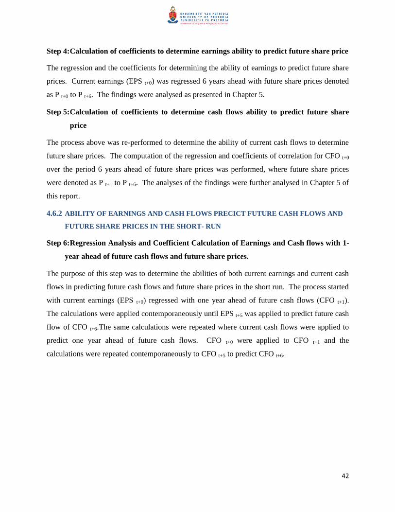
42
Step 4: Calculation of coefficients to determine earnings ability to predict future share price
The regression and the coefficients for determining the ability of earnings to predict future share
prices. Current earnings (EPS t+0) was regressed 6 years ahead with future share prices denoted
as P t+0 to P t+6. The findings were analysed as presented in Chapter 5.
Step 5: Calculation of coefficients to determine cash flows ability to predict future share
price
The process above was re-performed to determine the ability of current cash flows to determine
future share prices. The computation of the regression and coefficients of correlation for CFO t+0
over the period 6 years ahead of future share prices was performed, where future share prices
were denoted as P t+1 to P t+6. The analyses of the findings were further analysed in Chapter 5 of
this report.
4.6.2 ABILITY OF EARNINGS AND CASH FLOWS PRECICT FUTURE CASH FLOWS AND
FUTURE SHARE PRICES IN THE SHORT- RUN
Step 6: Regression Analysis and Coefficient Calculation of Earnings and Cash flows with 1-
year ahead of future cash flows and future share prices.
The purpose of this step was to determine the abilities of both current earnings and current cash
flows in predicting future cash flows and future share prices in the short run. The process started
with current earnings (EPS t+0) regressed with one year ahead of future cash flows (CFO t+1).
The calculations were applied contemporaneously until EPS t+5 was applied to predict future cash
flow of CFO t+6.The same calculations were repeated where current cash flows were applied to
predict one year ahead of future cash flows. CFO t+0 were applied to CFO t+1 and the
calculations were repeated contemporaneously to CFO t+5 to predict CFO t+6.
43
A similar process was replicated to predict future share prices applying current earnings and
current cash flows to 6 years ahead of future share prices. Again EPSt+0 and CFOt+0 were
contemporaneously applied to Pt+1 to Pt+6. For an example, EPSt+3 was regressed with Pt+4. The
objective of these predictive calculations was to assess the predictive abilities of current earnings
and current cash flows over future share prices. . Further analysis and interpretation of the
findings were presented in Chapter 5.
4.6.3 TESTING THE COEFICIENT OF CORRELATION
Step 7: Application of the coefficients to test the model’s explanatory power of future cash
flows and future share prices
The size of the APPENDICES was big and they were presented electronically.
(1) split the financial data on APPENDIX E into two categories. The first set being the first 39 companies and the second set being the 30 last companies.
(2) the financial data was "paired up" into EPS t+0 with CFO t+1. The pairing up was repeated up until EPS t+5 with CFO t+6. Similar process was repeated EPS t+0 with P t+1 and CFO t+0 with P t+1. The pocess was repreated until the 6th items was applied as the predicted item.
(3) the purpose of this step was to compute a REGRESSION ANALYSIS and the COEFFICIENTS that were applied to a model that was used to assess explanatory power of earnings and cash flows over future cash flows and future share prices.
(4) the confidence test for applying current cash flows contemparenously to CFO t+0 up to CFO t+ 6 was performed differently where the first 39 sets of data of CFO t+0, CFO t+2 and CFO t+4 were used as X variabless and CFOt+1, CFOt+3 and CFOt+5 were use as X variables to be predicted
(5) Excel Data Analysis 2 t-test were performed and results obtained are presented on Chapter 5 for earnings to future cash flows, earnings to future price, and cash flows to future price were performed to determine the t-statistic
44
4.7 LIMITATIONS
The following were the main key limitations encountered when the information was collected
and analysed:
McGregor BFA could not provide the financial information on a quarterly basis as per Kim
and Kross (2005) methodology. The share prices which were going to be tested with the
short term earnings or cash flow were only for the end financial year share prices.
The Statements of Cash flow presented by the JSE listed companies were prepared using
the Indirect Method. It should be remembered that Orpurt and Zang (2007) stated that
Direct Method was better a predictor of future cash flows than the Indirect Method. For
the purposes of the study, Indirect Method of the Statement of Cash Flow was used.
196 companies were eliminated from the population due to their financial information
being incomplete. The information provided of these companies was either the first time
financial information was presented after 2001 or the last information presented was before
2011. These findings limited the tests that were envisaged to be undertaken.
The test of Coefficient of Correlation of current cash flows contemporaneousness with one
year ahead future cash flows could not be performed due to the structure of the excel
spread-sheet.

45
Chapter 5
Results
In this chapter findings of the test results based on the regression analysis and t-tests and confidence of
coefficients are presented
46
5. RESULTS
5.1 INTRODUCTION
The research assessed the ability of current earnings and current cash flows from operations to
predict future cash flows and future share prices. The data was obtained from McGregor BFA
database which keeps the records of financial reports and financial information of the listed
companies. McGregor BFA provided 369 listed companies including both the main board and
the Alt X board. The sample selected ended up with 69 companies. This was after eliminating
the financial services companies, mining companies and the companies with incomplete financial
information.
The Excel worksheet was further analysed by applying the ―DATA ANALYSIS‖ tool on Excel
software. The tool allowed the computation of ―REGRESSION ANALYSIS‖ in order to test
the relationship between the financial variables as described above.
5.2 DESCRIPTIVE STATISTICS
Three Excel worksheets were prepared to show the EBITDA per SHARE (EPS), CASH FLOW
FROM OPERATIONS per SHARE (CFO) and SHARE PRICE which reflected the share price
as quoted on the JSE at financial year end of each company. The mean average of each financial
data for all 69 companies from 2001 to 2011 were summarised and presented here below:
This chapter of the research report provides the results of the findings and the statistical analysis
that were performed based on financial data collected through McGregor BFA for the period
from 2001 to 2011.
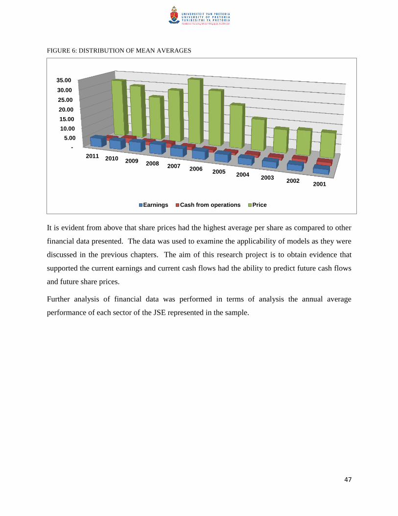
47
FIGURE 6: DISTRIBUTION OF MEAN AVERAGES
It is evident from above that share prices had the highest average per share as compared to other
financial data presented. The data was used to examine the applicability of models as they were
discussed in the previous chapters. The aim of this research project is to obtain evidence that
supported the current earnings and current cash flows had the ability to predict future cash flows
and future share prices.
Further analysis of financial data was performed in terms of analysis the annual average
performance of each sector of the JSE represented in the sample.
-
5.00
10.00
15.00
20.00
25.00
30.00
35.00
2011 2010 2009 2008 2007 20062005
20042003
20022001
Earnings Cash from operations Price
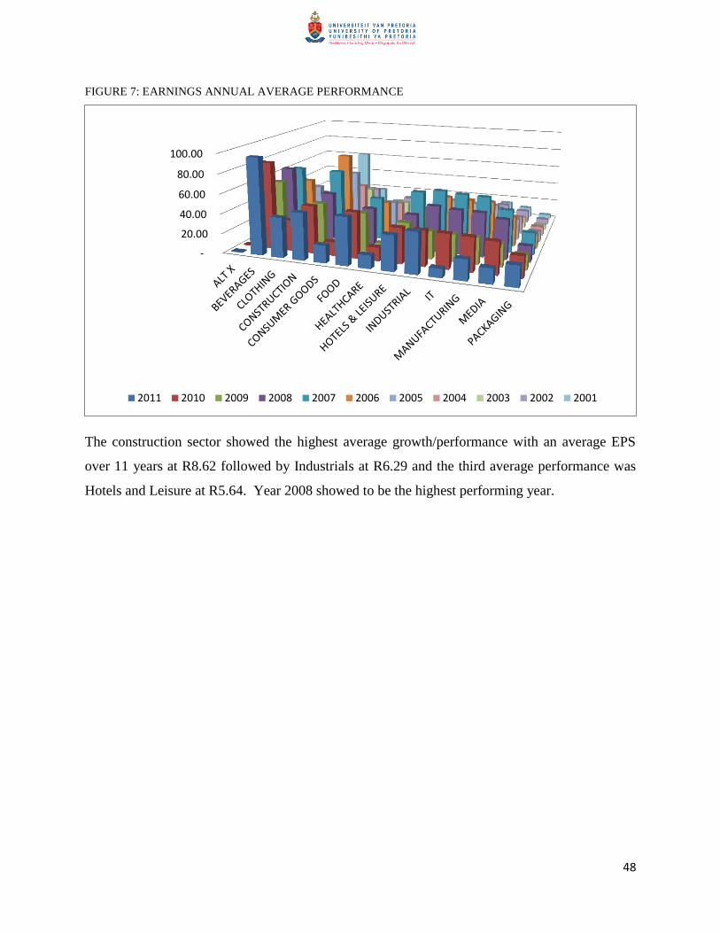
48
FIGURE 7: EARNINGS ANNUAL AVERAGE PERFORMANCE
The construction sector showed the highest average growth/performance with an average EPS
over 11 years at R8.62 followed by Industrials at R6.29 and the third average performance was
Hotels and Leisure at R5.64. Year 2008 showed to be the highest performing year.
-
20.00
40.00
60.00
80.00
100.00
2011 2010 2009 2008 2007 2006 2005 2004 2003 2002 2001
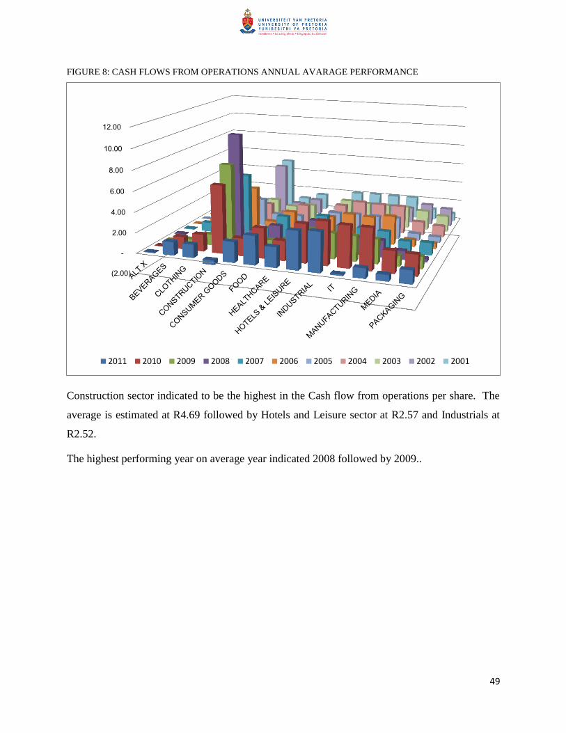
49
FIGURE 8: CASH FLOWS FROM OPERATIONS ANNUAL AVARAGE PERFORMANCE
Construction sector indicated to be the highest in the Cash flow from operations per share. The
average is estimated at R4.69 followed by Hotels and Leisure sector at R2.57 and Industrials at
R2.52.
The highest performing year on average year indicated 2008 followed by 2009..
(2.00)
-
2.00
4.00
6.00
8.00
10.00
12.00
2011 2010 2009 2008 2007 2006 2005 2004 2003 2002 2001

50
FIGURE 9: SHARE PRICES ANNUAL AVERAGE PERFORMANCE
The best performing sector in terms of share price performance was Beverages at R51.89 being
attributed mainly on SABMiller‘s share price. It was followed by the Construction sector with
an average performance of R46.11 and third rated performance was the Food sector with R31.19.
-
20.00
40.00
60.00
80.00
100.00
2011 2010 2009 2008 2007 2006 2005 2004 2003 2002 2001
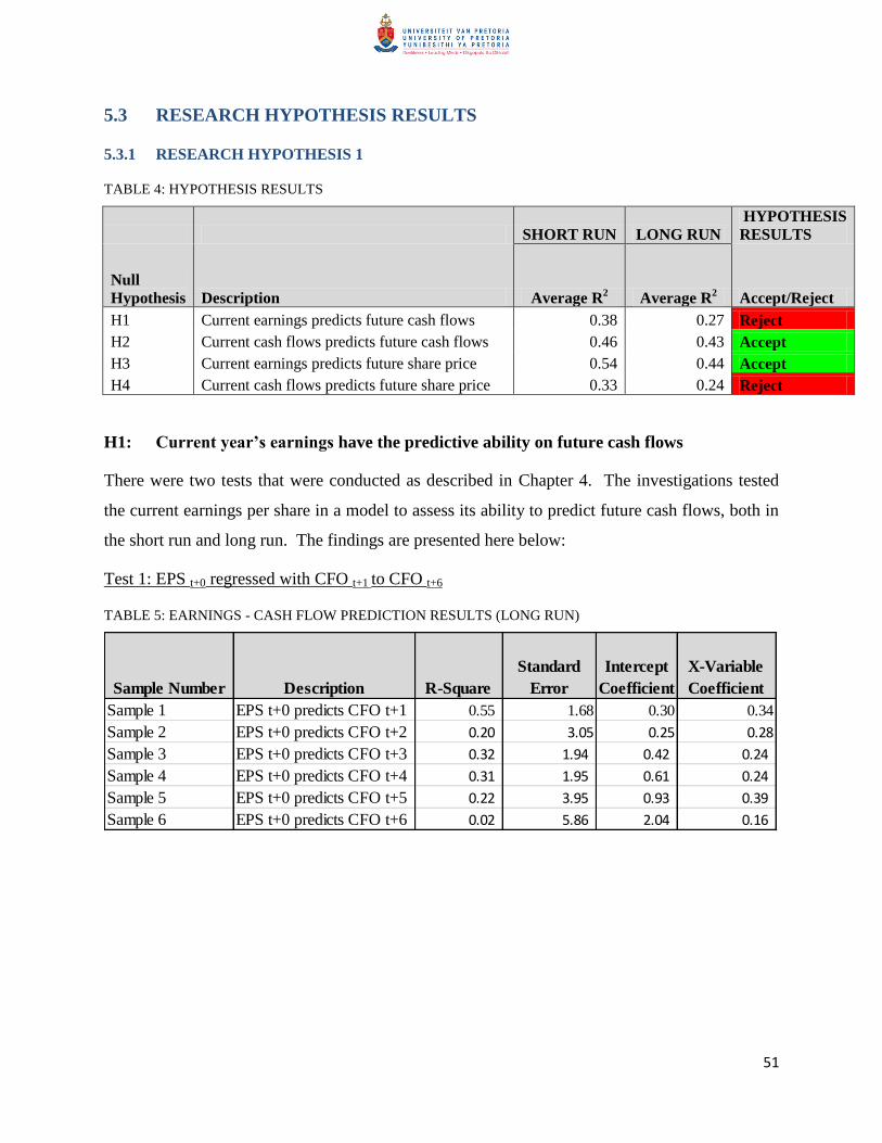
51
5.3 RESEARCH HYPOTHESIS RESULTS
5.3.1 RESEARCH HYPOTHESIS 1
TABLE 4: HYPOTHESIS RESULTS
SHORT RUN LONG RUN
HYPOTHESIS
RESULTS
Null
Hypothesis Description Average R2 Average R
2 Accept/Reject
H1 Current earnings predicts future cash flows 0.38 0.27 Reject
H2 Current cash flows predicts future cash flows 0.46 0.43 Accept
H3 Current earnings predicts future share price 0.54 0.44 Accept
H4 Current cash flows predicts future share price 0.33 0.24 Reject
H1: Current year’s earnings have the predictive ability on future cash flows
There were two tests that were conducted as described in Chapter 4. The investigations tested
the current earnings per share in a model to assess its ability to predict future cash flows, both in
the short run and long run. The findings are presented here below:
Test 1: EPS t+0 regressed with CFO t+1 to CFO t+6
TABLE 5: EARNINGS - CASH FLOW PREDICTION RESULTS (LONG RUN)
Sample Number Description R-Square
Standard
Error
Intercept
Coefficient
X-Variable
Coefficient
Sample 1 EPS t+0 predicts CFO t+1 0.55 1.68 0.30 0.34
Sample 2 EPS t+0 predicts CFO t+2 0.20 3.05 0.25 0.28
Sample 3 EPS t+0 predicts CFO t+3 0.32 1.94 0.42 0.24
Sample 4 EPS t+0 predicts CFO t+4 0.31 1.95 0.61 0.24
Sample 5 EPS t+0 predicts CFO t+5 0.22 3.95 0.93 0.39
Sample 6 EPS t+0 predicts CFO t+6 0.02 5.86 2.04 0.16
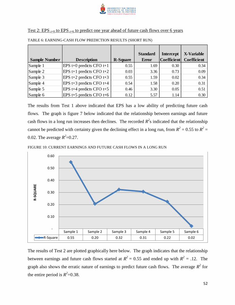
52
Test 2: EPS t+0 to EPS t+6 to predict one year ahead of future cash flows over 6 years
TABLE 6: EARNING-CASH FLOW PREDICTION RESULTS (SHORT RUN)
The results from Test 1 above indicated that EPS has a low ability of predicting future cash
flows. The graph is figure 7 below indicated that the relationship between earnings and future
cash flows in a long run increases then declines. The recorded R2s indicated that the relationship
cannot be predicted with certainty given the declining effect in a long run, from R2 = 0.55 to R
2 =
0.02. The average R2=0.27.
FIGURE 10: CURRENT EARNINGS AND FUTURE CASH FLOWS IN A LONG RUN
The results of Test 2 are plotted graphically here below. The graph indicates that the relationship
between earnings and future cash flows started at R2
= 0.55 and ended up with R2 = .12. The
graph also shows the erratic nature of earnings to predict future cash flows. The average R2 for
the entire period is R2=0.38.
Sample Number Description R-Square
Standard
Error
Intercept
Coefficient
X-Variable
Coefficient
Sample 1 EPS t+0 predicts CFO t+1 0.55 1.69 0.30 0.34
Sample 2 EPS t+1 predicts CFO t+2 0.03 3.36 0.73 0.09
Sample 3 EPS t+2 predicts CFO t+3 0.55 1.59 0.02 0.34
Sample 4 EPS t+3 predicts CFO t+4 0.54 1.58 0.20 0.31
Sample 5 EPS t+4 predicts CFO t+5 0.46 3.30 0.05 0.51
Sample 6 EPS t+5 predicts CFO t+6 0.12 5.57 1.14 0.30
Sample 1 Sample 2 Sample 3 Sample 4 Sample 5 Sample 6
R-Square 0.55 0.20 0.32 0.31 0.22 0.02
-
0.10
0.20
0.30
0.40
0.50
0.60
R-S
QU
AR
E
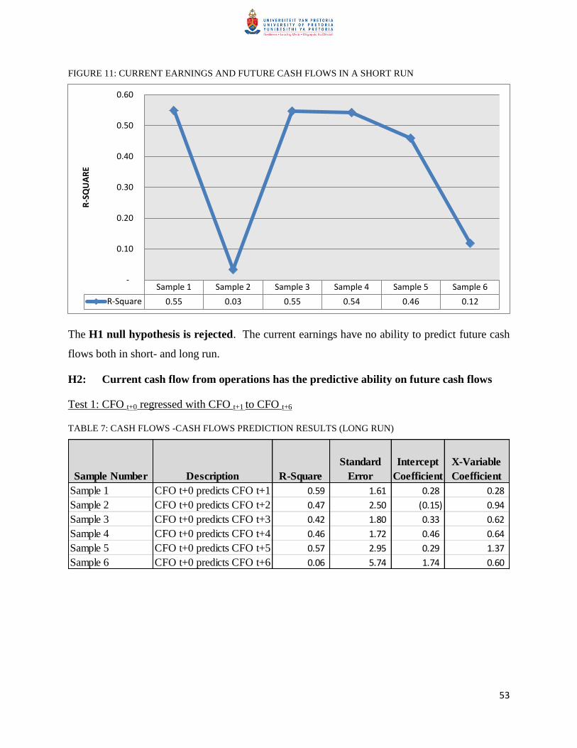
53
FIGURE 11: CURRENT EARNINGS AND FUTURE CASH FLOWS IN A SHORT RUN
The H1 null hypothesis is rejected. The current earnings have no ability to predict future cash
flows both in short- and long run.
H2: Current cash flow from operations has the predictive ability on future cash flows
Test 1: CFO t+0 regressed with CFO t+1 to CFO t+6
TABLE 7: CASH FLOWS -CASH FLOWS PREDICTION RESULTS (LONG RUN)
Sample 1 Sample 2 Sample 3 Sample 4 Sample 5 Sample 6
R-Square 0.55 0.03 0.55 0.54 0.46 0.12
-
0.10
0.20
0.30
0.40
0.50
0.60R
-SQ
UA
RE
Sample Number Description R-Square
Standard
Error
Intercept
Coefficient
X-Variable
Coefficient
Sample 1 CFO t+0 predicts CFO t+1 0.59 1.61 0.28 0.28
Sample 2 CFO t+0 predicts CFO t+2 0.47 2.50 (0.15) 0.94
Sample 3 CFO t+0 predicts CFO t+3 0.42 1.80 0.33 0.62
Sample 4 CFO t+0 predicts CFO t+4 0.46 1.72 0.46 0.64
Sample 5 CFO t+0 predicts CFO t+5 0.57 2.95 0.29 1.37
Sample 6 CFO t+0 predicts CFO t+6 0.06 5.74 1.74 0.60
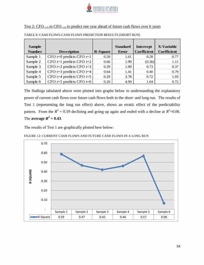
54
Test 2: CFO t+0 to CFO t+6 to predict one year ahead of future cash flows over 6 years
TABLE 8: CASH FLOWS-CASH FLOWS PREDICTION RESULTS (SHORT RUN)
The findings tabulated above were plotted into graphs below to understanding the explanatory
power of current cash flows over future cash flows both in the short- and long run. The results of
Test 1 (representing the long run effect) above, shows an erratic effect of the predictability
pattern. From the R2 = 0.59 declining and going up again and ended with a decline at R
2=0.06.
The average R2 = 0.43.
The results of Test 1 are graphically plotted here below:
FIGURE 12: CURRENT CASH FLOWS AND FUTURE CASH FLOWS IN A LONG RUN
Sample
Number Description R-Square
Standard
Error
Intercept
Coefficient
X-Variable
Coefficient
Sample 1 CFO t+0 predicts CFO t+1 0.59 1.61 0.28 0.77
Sample 2 CFO t+1 predicts CFO t+2 0.66 1.99 (0.36) 1.11
Sample 3 CFO t+2 predicts CFO t+3 0.29 1.99 0.73 0.37
Sample 4 CFO t+3 predicts CFO t+4 0.64 1.41 0.40 0.79
Sample 5 CFO t+4 predicts CFO t+5 0.29 3.78 0.72 1.03
Sample 6 CFO t+5 predicts CFO t+6 0.29 4.99 1.04 0.72
Sample 1 Sample 2 Sample 3 Sample 4 Sample 5 Sample 6
R-Square 0.59 0.47 0.42 0.46 0.57 0.06
-
0.10
0.20
0.30
0.40
0.50
0.60
0.70
R-S
QU
AR
E
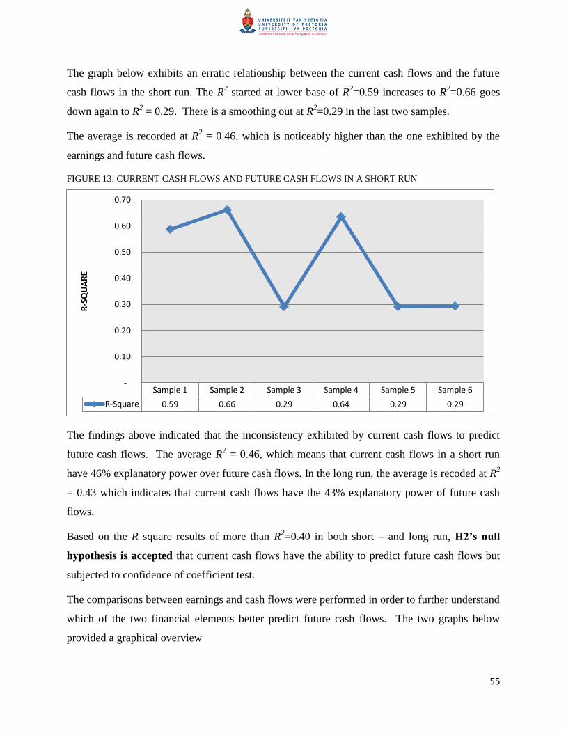
55
The graph below exhibits an erratic relationship between the current cash flows and the future
cash flows in the short run. The R2 started at lower base of R
2=0.59 increases to R
2=0.66 goes
down again to R2 = 0.29. There is a smoothing out at R
2=0.29 in the last two samples.
The average is recorded at R2 = 0.46, which is noticeably higher than the one exhibited by the
earnings and future cash flows.
FIGURE 13: CURRENT CASH FLOWS AND FUTURE CASH FLOWS IN A SHORT RUN
The findings above indicated that the inconsistency exhibited by current cash flows to predict
future cash flows. The average R2 = 0.46, which means that current cash flows in a short run
have 46% explanatory power over future cash flows. In the long run, the average is recoded at R2
= 0.43 which indicates that current cash flows have the 43% explanatory power of future cash
flows.
Based on the R square results of more than R2=0.40 in both short – and long run, H2’s null
hypothesis is accepted that current cash flows have the ability to predict future cash flows but
subjected to confidence of coefficient test.
The comparisons between earnings and cash flows were performed in order to further understand
which of the two financial elements better predict future cash flows. The two graphs below
provided a graphical overview
Sample 1 Sample 2 Sample 3 Sample 4 Sample 5 Sample 6
R-Square 0.59 0.66 0.29 0.64 0.29 0.29
-
0.10
0.20
0.30
0.40
0.50
0.60
0.70
R-S
QU
AR
E
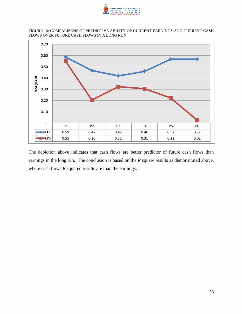
56
FIGURE 14: COMPARISONS OF PREDICTIVE ABILITY OF CURRENT EARNINGS AND CURRENT CASH
FLOWS OVER FUTURE CASH FLOWS IN A LONG RUN
The depiction above indicates that cash flows are better predictor of future cash flows than
earnings in the long run. The conclusion is based on the R square results as demonstrated above,
where cash flows R squared results are than the earnings.
P1 P2 P3 P4 P5 P6
CFO 0.59 0.47 0.42 0.46 0.57 0.57
EPS 0.55 0.20 0.32 0.31 0.22 0.02
-
0.10
0.20
0.30
0.40
0.50
0.60
0.70
R-S
QU
AR
E
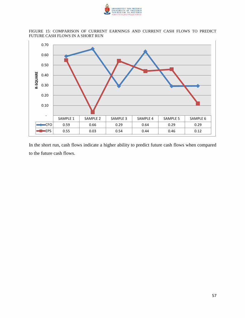
57
FIGURE 15: COMPARISON OF CURRENT EARNINGS AND CURRENT CASH FLOWS TO PREDICT
FUTURE CASH FLOWS IN A SHORT RUN
In the short run, cash flows indicate a higher ability to predict future cash flows when compared
to the future cash flows.
SAMPLE 1 SAMPLE 2 SAMPLE 3 SAMPLE 4 SAMPLE 5 SAMPLE 6
CFO 0.59 0.66 0.29 0.64 0.29 0.29
EPS 0.55 0.03 0.54 0.44 0.46 0.12
-
0.10
0.20
0.30
0.40
0.50
0.60
0.70
R-S
QU
AR
E
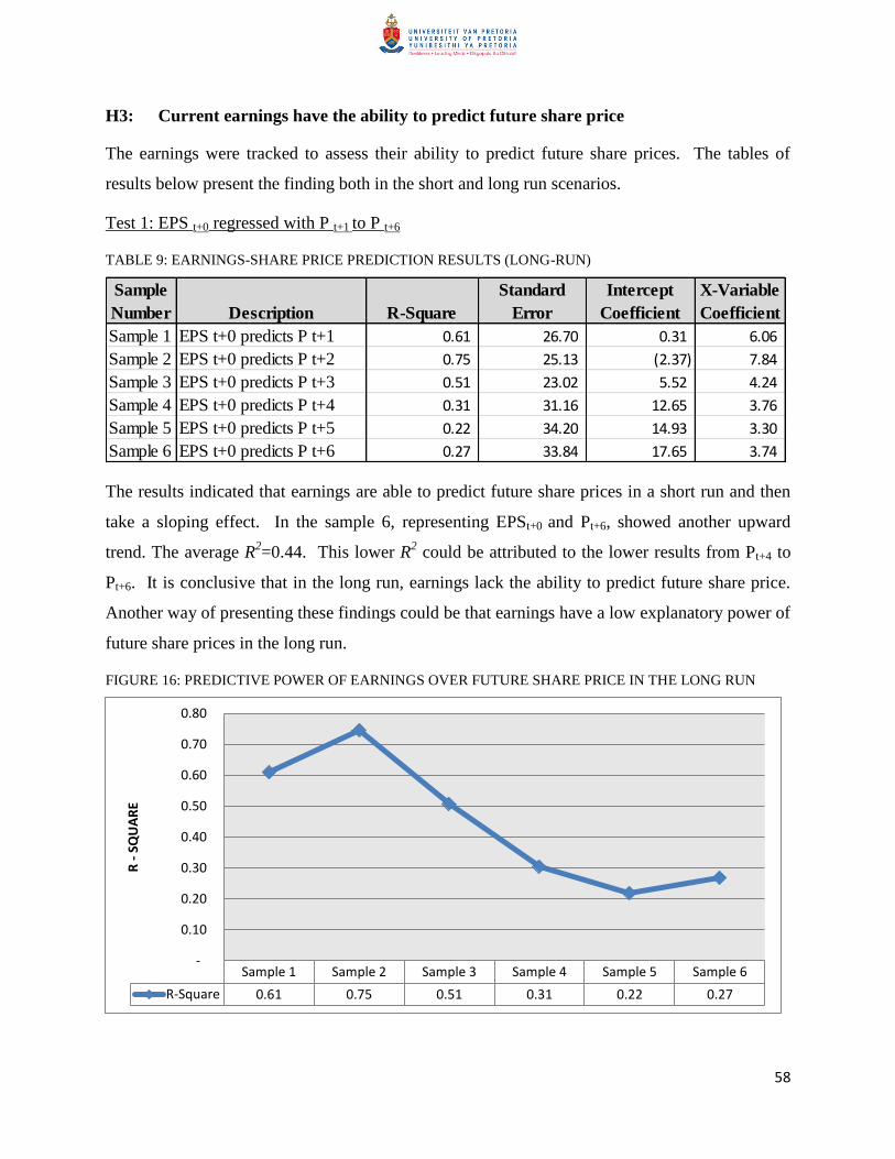
58
H3: Current earnings have the ability to predict future share price
The earnings were tracked to assess their ability to predict future share prices. The tables of
results below present the finding both in the short and long run scenarios.
Test 1: EPS t+0 regressed with P t+1 to P t+6
TABLE 9: EARNINGS-SHARE PRICE PREDICTION RESULTS (LONG-RUN)
The results indicated that earnings are able to predict future share prices in a short run and then
take a sloping effect. In the sample 6, representing EPSt+0 and Pt+6, showed another upward
trend. The average R2=0.44. This lower R
2 could be attributed to the lower results from Pt+4 to
Pt+6. It is conclusive that in the long run, earnings lack the ability to predict future share price.
Another way of presenting these findings could be that earnings have a low explanatory power of
future share prices in the long run.
FIGURE 16: PREDICTIVE POWER OF EARNINGS OVER FUTURE SHARE PRICE IN THE LONG RUN
Sample
Number Description R-Square
Standard
Error
Intercept
Coefficient
X-Variable
Coefficient
Sample 1 EPS t+0 predicts P t+1 0.61 26.70 0.31 6.06
Sample 2 EPS t+0 predicts P t+2 0.75 25.13 (2.37) 7.84
Sample 3 EPS t+0 predicts P t+3 0.51 23.02 5.52 4.24
Sample 4 EPS t+0 predicts P t+4 0.31 31.16 12.65 3.76
Sample 5 EPS t+0 predicts P t+5 0.22 34.20 14.93 3.30
Sample 6 EPS t+0 predicts P t+6 0.27 33.84 17.65 3.74
Sample 1 Sample 2 Sample 3 Sample 4 Sample 5 Sample 6
R-Square 0.61 0.75 0.51 0.31 0.22 0.27
-
0.10
0.20
0.30
0.40
0.50
0.60
0.70
0.80
R -
SQ
UA
RE
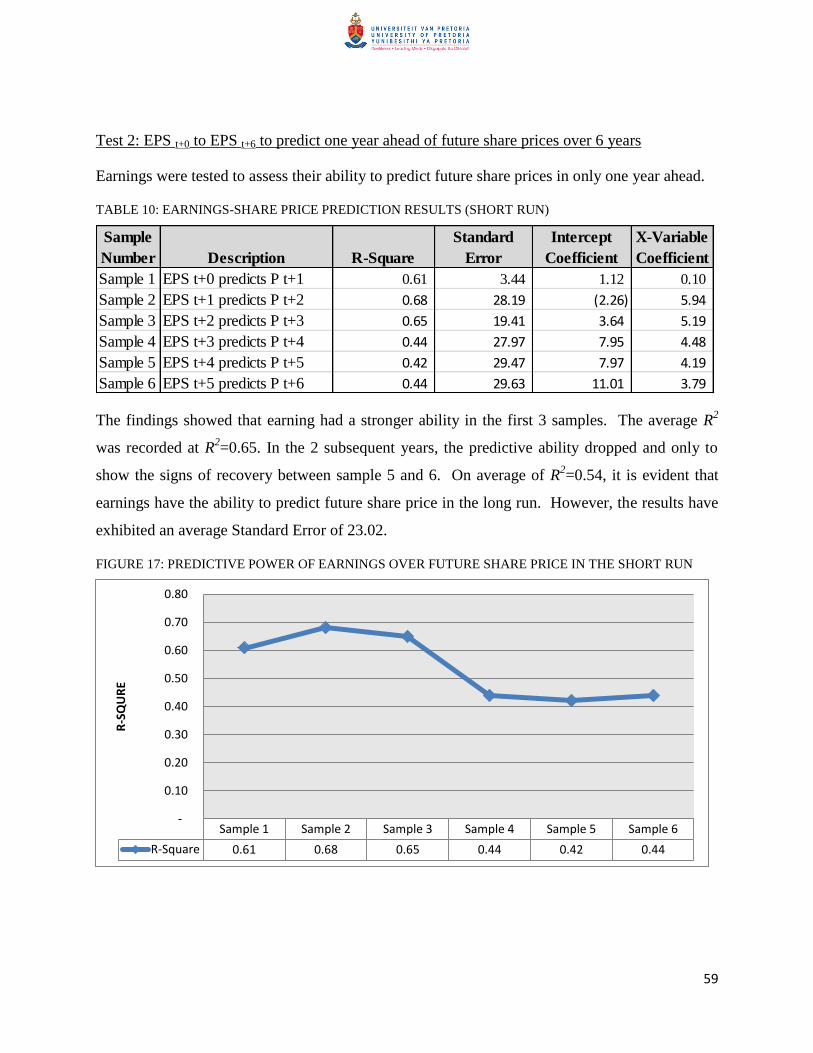
59
Test 2: EPS t+0 to EPS t+6 to predict one year ahead of future share prices over 6 years
Earnings were tested to assess their ability to predict future share prices in only one year ahead.
TABLE 10: EARNINGS-SHARE PRICE PREDICTION RESULTS (SHORT RUN)
The findings showed that earning had a stronger ability in the first 3 samples. The average R2
was recorded at R2=0.65. In the 2 subsequent years, the predictive ability dropped and only to
show the signs of recovery between sample 5 and 6. On average of R2=0.54, it is evident that
earnings have the ability to predict future share price in the long run. However, the results have
exhibited an average Standard Error of 23.02.
FIGURE 17: PREDICTIVE POWER OF EARNINGS OVER FUTURE SHARE PRICE IN THE SHORT RUN
Sample
Number Description R-Square
Standard
Error
Intercept
Coefficient
X-Variable
Coefficient
Sample 1 EPS t+0 predicts P t+1 0.61 3.44 1.12 0.10
Sample 2 EPS t+1 predicts P t+2 0.68 28.19 (2.26) 5.94
Sample 3 EPS t+2 predicts P t+3 0.65 19.41 3.64 5.19
Sample 4 EPS t+3 predicts P t+4 0.44 27.97 7.95 4.48
Sample 5 EPS t+4 predicts P t+5 0.42 29.47 7.97 4.19
Sample 6 EPS t+5 predicts P t+6 0.44 29.63 11.01 3.79
Sample 1 Sample 2 Sample 3 Sample 4 Sample 5 Sample 6
R-Square 0.61 0.68 0.65 0.44 0.42 0.44
-
0.10
0.20
0.30
0.40
0.50
0.60
0.70
0.80
R-S
QU
RE
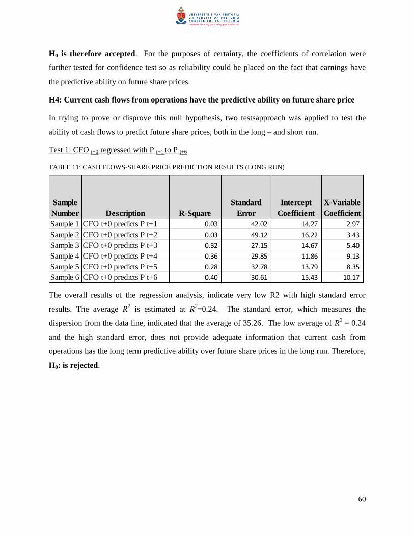
60
H0 is therefore accepted. For the purposes of certainty, the coefficients of correlation were
further tested for confidence test so as reliability could be placed on the fact that earnings have
the predictive ability on future share prices.
H4: Current cash flows from operations have the predictive ability on future share price
In trying to prove or disprove this null hypothesis, two testsapproach was applied to test the
ability of cash flows to predict future share prices, both in the long – and short run.
Test 1: CFO t+0 regressed with P t+1 to P t+6
TABLE 11: CASH FLOWS-SHARE PRICE PREDICTION RESULTS (LONG RUN)
The overall results of the regression analysis, indicate very low R2 with high standard error
results. The average R2 is estimated at R
2=0.24. The standard error, which measures the
dispersion from the data line, indicated that the average of 35.26. The low average of R2 = 0.24
and the high standard error, does not provide adequate information that current cash from
operations has the long term predictive ability over future share prices in the long run. Therefore,
H0: is rejected.
Sample
Number Description R-Square
Standard
Error
Intercept
Coefficient
X-Variable
Coefficient
Sample 1 CFO t+0 predicts P t+1 0.03 42.02 14.27 2.97
Sample 2 CFO t+0 predicts P t+2 0.03 49.12 16.22 3.43
Sample 3 CFO t+0 predicts P t+3 0.32 27.15 14.67 5.40
Sample 4 CFO t+0 predicts P t+4 0.36 29.85 11.86 9.13
Sample 5 CFO t+0 predicts P t+5 0.28 32.78 13.79 8.35
Sample 6 CFO t+0 predicts P t+6 0.40 30.61 15.43 10.17
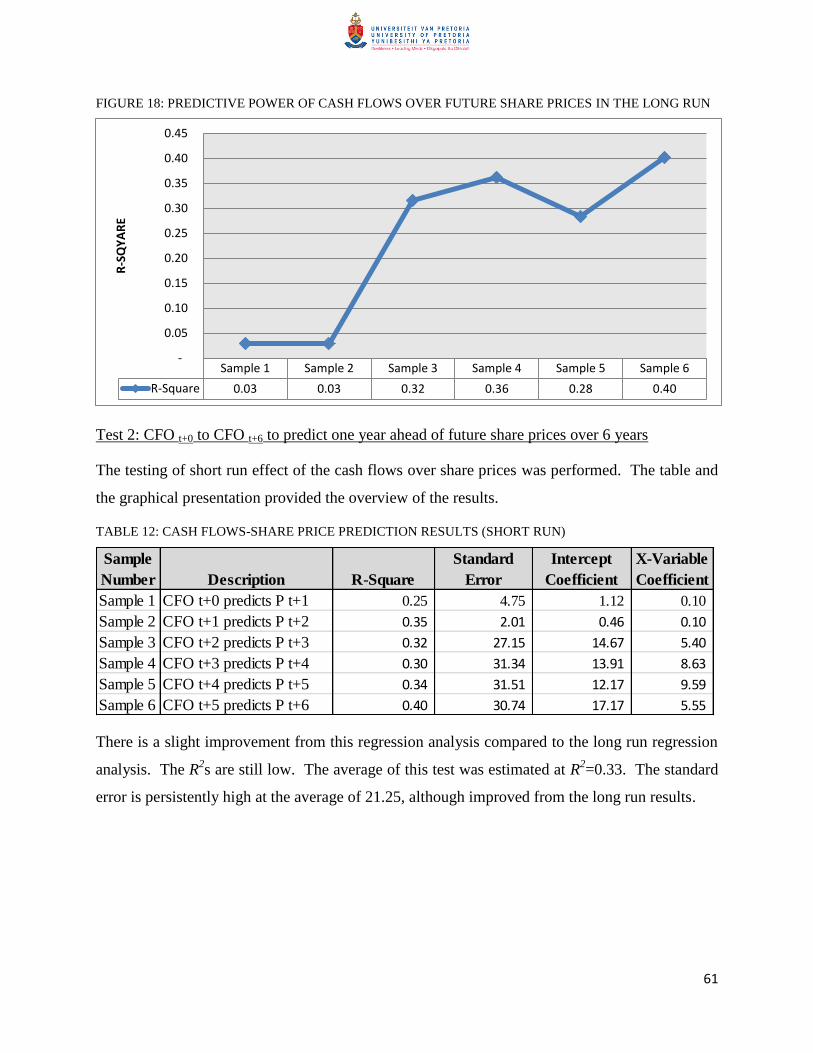
61
FIGURE 18: PREDICTIVE POWER OF CASH FLOWS OVER FUTURE SHARE PRICES IN THE LONG RUN
Test 2: CFO t+0 to CFO t+6 to predict one year ahead of future share prices over 6 years
The testing of short run effect of the cash flows over share prices was performed. The table and
the graphical presentation provided the overview of the results.
TABLE 12: CASH FLOWS-SHARE PRICE PREDICTION RESULTS (SHORT RUN)
There is a slight improvement from this regression analysis compared to the long run regression
analysis. The R2s are still low. The average of this test was estimated at R
2=0.33. The standard
error is persistently high at the average of 21.25, although improved from the long run results.
Sample 1 Sample 2 Sample 3 Sample 4 Sample 5 Sample 6
R-Square 0.03 0.03 0.32 0.36 0.28 0.40
-
0.05
0.10
0.15
0.20
0.25
0.30
0.35
0.40
0.45R
-SQ
YA
RE
Sample
Number Description R-Square
Standard
Error
Intercept
Coefficient
X-Variable
Coefficient
Sample 1 CFO t+0 predicts P t+1 0.25 4.75 1.12 0.10
Sample 2 CFO t+1 predicts P t+2 0.35 2.01 0.46 0.10
Sample 3 CFO t+2 predicts P t+3 0.32 27.15 14.67 5.40
Sample 4 CFO t+3 predicts P t+4 0.30 31.34 13.91 8.63
Sample 5 CFO t+4 predicts P t+5 0.34 31.51 12.17 9.59
Sample 6 CFO t+5 predicts P t+6 0.40 30.74 17.17 5.55
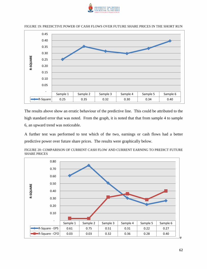
62
FIGURE 19: PREDICTIVE POWER OF CASH FLOWS OVER FUTURE SHARE PRICES IN THE SHORT RUN
The results above show an erratic behaviour of the predictive line. This could be attributed to the
high standard error that was noted. From the graph, it is noted that that from sample 4 to sample
6, an upward trend was noticeable.
A further test was performed to test which of the two, earnings or cash flows had a better
predictive power over future share prices. The results were graphically below.
FIGURE 20: COMPARISON OF CURRENT CASH FLOW AND CURRENT EARNING TO PREDICT FUTURE
SHARE PRICES
e
Sample 1 Sample 2 Sample 3 Sample 4 Sample 5 Sample 6
R-Square 0.25 0.35 0.32 0.30 0.34 0.40
-
0.05
0.10
0.15
0.20
0.25
0.30
0.35
0.40
0.45R
-SQ
UA
RE
Sample 1 Sample 2 Sample 3 Sample 4 Sample 5 Sample 6
R-Square - EPS 0.61 0.75 0.51 0.31 0.22 0.27
R-Square - CFO 0.03 0.03 0.32 0.36 0.28 0.40
-
0.10
0.20
0.30
0.40
0.50
0.60
0.70
0.80
R-S
QU
AR
E
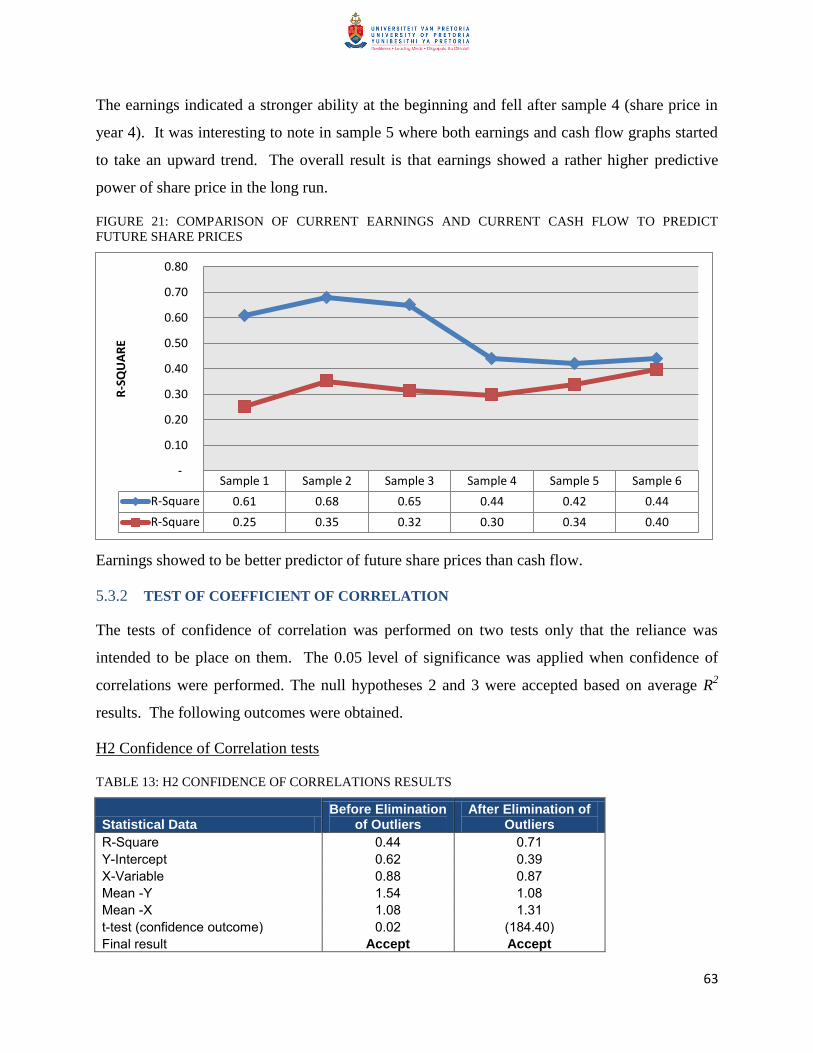
63
The earnings indicated a stronger ability at the beginning and fell after sample 4 (share price in
year 4). It was interesting to note in sample 5 where both earnings and cash flow graphs started
to take an upward trend. The overall result is that earnings showed a rather higher predictive
power of share price in the long run.
FIGURE 21: COMPARISON OF CURRENT EARNINGS AND CURRENT CASH FLOW TO PREDICT
FUTURE SHARE PRICES
Earnings showed to be better predictor of future share prices than cash flow.
5.3.2 TEST OF COEFFICIENT OF CORRELATION
The tests of confidence of correlation was performed on two tests only that the reliance was
intended to be place on them. The 0.05 level of significance was applied when confidence of
correlations were performed. The null hypotheses 2 and 3 were accepted based on average R2
results. The following outcomes were obtained.
H2 Confidence of Correlation tests
TABLE 13: H2 CONFIDENCE OF CORRELATIONS RESULTS
Statistical Data Before Elimination
of Outliers After Elimination of
Outliers
R-Square 0.44 0.71
Y-Intercept 0.62 0.39
X-Variable 0.88 0.87
Mean -Y 1.54 1.08
Mean -X 1.08 1.31
t-test (confidence outcome) 0.02 (184.40)
Final result Accept Accept
Sample 1 Sample 2 Sample 3 Sample 4 Sample 5 Sample 6
R-Square 0.61 0.68 0.65 0.44 0.42 0.44
R-Square 0.25 0.35 0.32 0.30 0.34 0.40
-
0.10
0.20
0.30
0.40
0.50
0.60
0.70
0.80
R-S
QU
AR
E
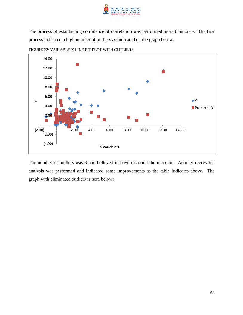
64
The process of establishing confidence of correlation was performed more than once. The first
process indicated a high number of outliers as indicated on the graph below:
FIGURE 22: VARIABLE X LINE FIT PLOT WITH OUTLIERS
The number of outliers was 8 and believed to have distorted the outcome. Another regression
analysis was performed and indicated some improvements as the table indicates above. The
graph with eliminated outliers is here below:
(4.00)
(2.00)
-
2.00
4.00
6.00
8.00
10.00
12.00
14.00
(2.00) - 2.00 4.00 6.00 8.00 10.00 12.00 14.00
Y
X Variable 1
Y
Predicted Y
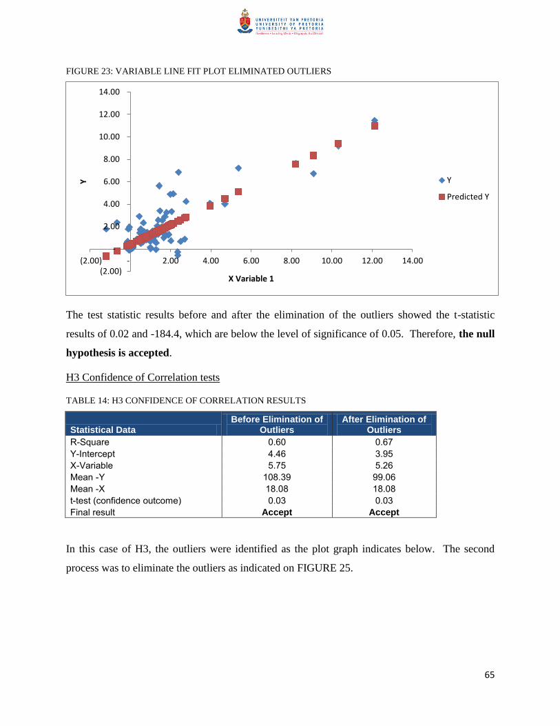
65
FIGURE 23: VARIABLE LINE FIT PLOT ELIMINATED OUTLIERS
The test statistic results before and after the elimination of the outliers showed the t-statistic
results of 0.02 and -184.4, which are below the level of significance of 0.05. Therefore, the null
hypothesis is accepted.
H3 Confidence of Correlation tests
TABLE 14: H3 CONFIDENCE OF CORRELATION RESULTS
Statistical Data Before Elimination of
Outliers After Elimination of
Outliers
R-Square 0.60 0.67
Y-Intercept 4.46 3.95
X-Variable 5.75 5.26
Mean -Y 108.39 99.06
Mean -X 18.08 18.08
t-test (confidence outcome) 0.03 0.03
Final result Accept Accept
In this case of H3, the outliers were identified as the plot graph indicates below. The second
process was to eliminate the outliers as indicated on FIGURE 25.
(2.00)
-
2.00
4.00
6.00
8.00
10.00
12.00
14.00
(2.00) - 2.00 4.00 6.00 8.00 10.00 12.00 14.00
Y
X Variable 1
Y
Predicted Y
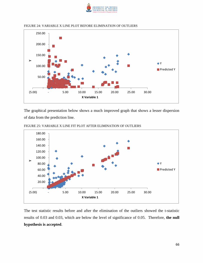
66
FIGURE 24: VARIABLE X LINE PLOT BEFORE ELIMINATION OF OUTLIERS
The graphical presentation below shows a much improved graph that shows a lesser dispersion
of data from the prediction line.
FIGURE 25: VARIABLE X LINE FIT PLOT AFTER ELIMINATION OF OUTLIERS
The test statistic results before and after the elimination of the outliers showed the t-statistic
results of 0.03 and 0.03, which are below the level of significance of 0.05. Therefore, the null
hypothesis is accepted.
-
50.00
100.00
150.00
200.00
250.00
(5.00) - 5.00 10.00 15.00 20.00 25.00 30.00
Y
X Variable 1
Y
Predicted Y
-
20.00
40.00
60.00
80.00
100.00
120.00
140.00
160.00
180.00
(5.00) - 5.00 10.00 15.00 20.00 25.00 30.00
Y
X Variable 1
Y
Predicted Y

67
Chapter 6
Discussion
This chapter discusses the hypotheses findings and elaborates more on the results.
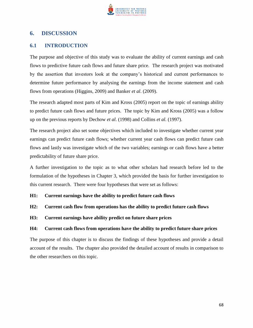
68
6. DISCUSSION
6.1 INTRODUCTION
The purpose and objective of this study was to evaluate the ability of current earnings and cash
flows to predictive future cash flows and future share price. The research project was motivated
by the assertion that investors look at the company‘s historical and current performances to
determine future performance by analysing the earnings from the income statement and cash
flows from operations (Higgins, 2009) and Banker et al. (2009).
The research adapted most parts of Kim and Kross (2005) report on the topic of earnings ability
to predict future cash flows and future prices. The topic by Kim and Kross (2005) was a follow
up on the previous reports by Dechow et al. (1998) and Collins et al. (1997).
The research project also set some objectives which included to investigate whether current year
earnings can predict future cash flows; whether current year cash flows can predict future cash
flows and lastly was investigate which of the two variables; earnings or cash flows have a better
predictability of future share price.
A further investigation to the topic as to what other scholars had research before led to the
formulation of the hypotheses in Chapter 3, which provided the basis for further investigation to
this current research. There were four hypotheses that were set as follows:
H1: Current earnings have the ability to predict future cash flows
H2: Current cash flow from operations has the ability to predict future cash flows
H3: Current earnings have ability predict on future share prices
H4: Current cash flows from operations have the ability to predict future share prices
The purpose of this chapter is to discuss the findings of these hypotheses and provide a detail
account of the results. The chapter also provided the detailed account of results in comparison to
the other researchers on this topic.
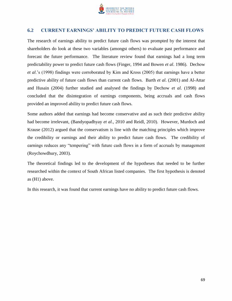
69
6.2 CURRENT EARNINGS’ ABILITY TO PREDICT FUTURE CASH FLOWS
The research of earnings ability to predict future cash flows was prompted by the interest that
shareholders do look at these two variables (amongst others) to evaluate past performance and
forecast the future performance. The literature review found that earnings had a long term
predictability power to predict future cash flows (Finger, 1994 and Bowen et al. 1986). Dechow
et al.‘s (1998) findings were corroborated by Kim and Kross (2005) that earnings have a better
predictive ability of future cash flows than current cash flows. Barth et al. (2001) and Al-Attar
and Husain (2004) further studied and analysed the findings by Dechow et al. (1998) and
concluded that the disintegration of earnings components, being accruals and cash flows
provided an improved ability to predict future cash flows.
Some authors added that earnings had become conservative and as such their predictive ability
had become irrelevant, (Bandyopadhyay et al., 2010 and Reidl, 2010). However, Murdoch and
Krause (2012) argued that the conservatism is line with the matching principles which improve
the credibility or earnings and their ability to predict future cash flows. The credibility of
earnings reduces any ―tempering‖ with future cash flows in a form of accruals by management
(Roychowdhury, 2003).
The theoretical findings led to the development of the hypotheses that needed to be further
researched within the context of South African listed companies. The first hypothesis is denoted
as (H1) above.
In this research, it was found that current earnings have no ability to predict future cash flows.
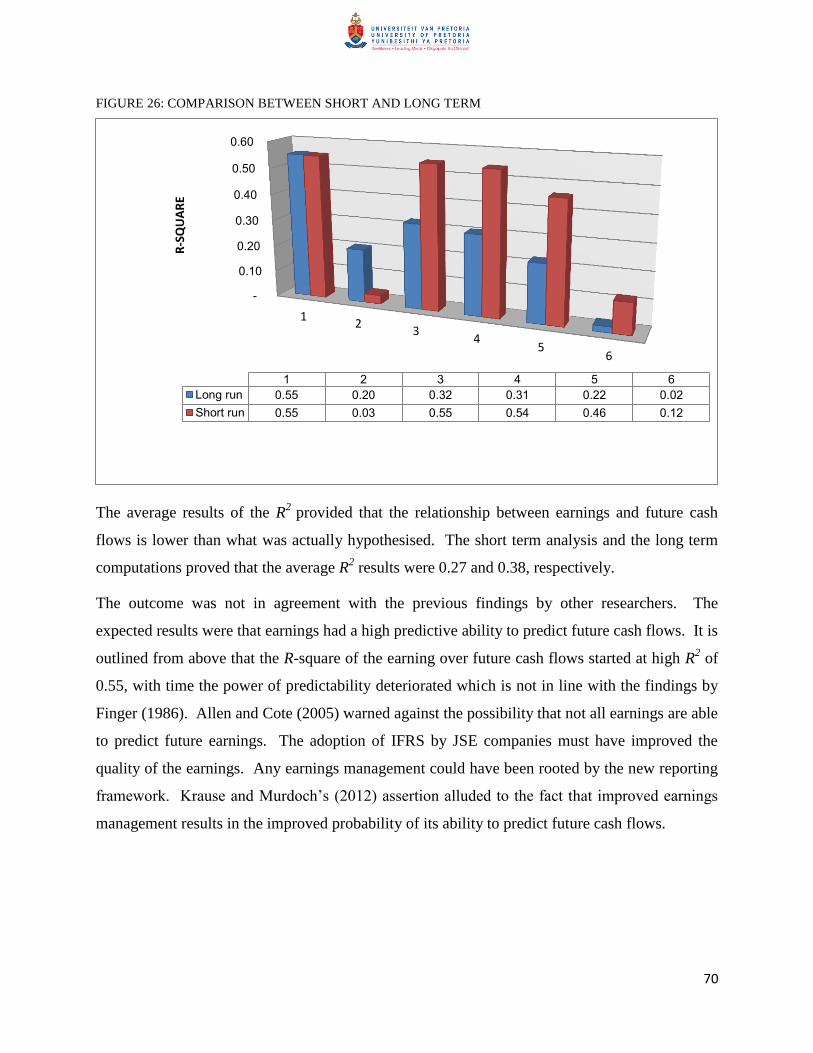
70
FIGURE 26: COMPARISON BETWEEN SHORT AND LONG TERM
The average results of the R2
provided that the relationship between earnings and future cash
flows is lower than what was actually hypothesised. The short term analysis and the long term
computations proved that the average R2 results were 0.27 and 0.38, respectively.
The outcome was not in agreement with the previous findings by other researchers. The
expected results were that earnings had a high predictive ability to predict future cash flows. It is
outlined from above that the R-square of the earning over future cash flows started at high R2 of
0.55, with time the power of predictability deteriorated which is not in line with the findings by
Finger (1986). Allen and Cote (2005) warned against the possibility that not all earnings are able
to predict future earnings. The adoption of IFRS by JSE companies must have improved the
quality of the earnings. Any earnings management could have been rooted by the new reporting
framework. Krause and Murdoch‘s (2012) assertion alluded to the fact that improved earnings
management results in the improved probability of its ability to predict future cash flows.
-
0.10
0.20
0.30
0.40
0.50
0.60
12
34
56
R-S
QU
AR
E
1 2 3 4 5 6
Long run 0.55 0.20 0.32 0.31 0.22 0.02
Short run 0.55 0.03 0.55 0.54 0.46 0.12
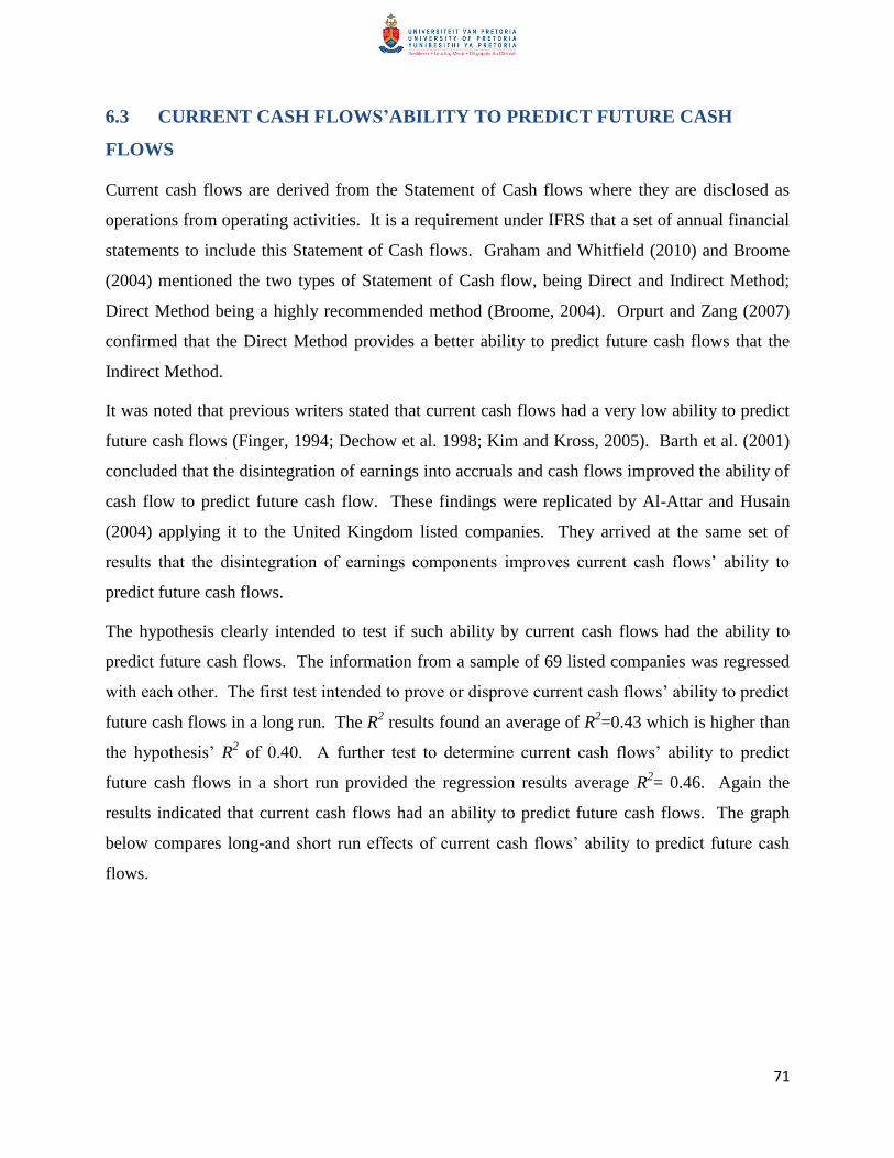
71
6.3 CURRENT CASH FLOWS’ABILITY TO PREDICT FUTURE CASH
FLOWS
Current cash flows are derived from the Statement of Cash flows where they are disclosed as
operations from operating activities. It is a requirement under IFRS that a set of annual financial
statements to include this Statement of Cash flows. Graham and Whitfield (2010) and Broome
(2004) mentioned the two types of Statement of Cash flow, being Direct and Indirect Method;
Direct Method being a highly recommended method (Broome, 2004). Orpurt and Zang (2007)
confirmed that the Direct Method provides a better ability to predict future cash flows that the
Indirect Method.
It was noted that previous writers stated that current cash flows had a very low ability to predict
future cash flows (Finger, 1994; Dechow et al. 1998; Kim and Kross, 2005). Barth et al. (2001)
concluded that the disintegration of earnings into accruals and cash flows improved the ability of
cash flow to predict future cash flow. These findings were replicated by Al-Attar and Husain
(2004) applying it to the United Kingdom listed companies. They arrived at the same set of
results that the disintegration of earnings components improves current cash flows‘ ability to
predict future cash flows.
The hypothesis clearly intended to test if such ability by current cash flows had the ability to
predict future cash flows. The information from a sample of 69 listed companies was regressed
with each other. The first test intended to prove or disprove current cash flows‘ ability to predict
future cash flows in a long run. The R2 results found an average of R
2=0.43 which is higher than
the hypothesis‘ R2 of 0.40. A further test to determine current cash flows‘ ability to predict
future cash flows in a short run provided the regression results average R2= 0.46. Again the
results indicated that current cash flows had an ability to predict future cash flows. The graph
below compares long-and short run effects of current cash flows‘ ability to predict future cash
flows.
72
FIGURE 27: COMPARISON BETWEEN SHORT RUN AND LONG RUN
The regression results suggested the null hypothesis be accepted. The test results were further
subjected to a confidence of coefficients test to ensure that the results obtained could provide
same results with an independent data. At significant level of 0.05, the t-test result was equal to
0.01613536 before the elimination of outliers; after the elimination, the t-test result was
(184.399978). Both t-test results were lower than 0.05 and the R2 results improved from 0.44 to
0.71.
The results provided by these tests that were performed indicate that current cash flows have the
ability to predict future cash flows both in the short- and ling run. The null hypothesis was
accepted.
The tests results are in contradiction to what the previous scholars have presented. Dechow et al.
(1998) and Kim and Kross (2005) research findings concluded that current cash flows had a
lower ability to predict future cash flows. The findings are in contradiction with the findings by
Finger (1994). The assertion by Orpurt and Zang (2007) that the Direct Method of Statement of
Cash flow was better predictor of future cash flow could not be proved due to the fact that the
companies in the tests use the Indirect Method.
-
0.10
0.20
0.30
0.40
0.50
0.60
0.70
12
34
56
R-S
QU
AR
E
1 2 3 4 5 6
Long Run 0.59 0.47 0.42 0.46 0.57 0.06
Short run 0.59 0.66 0.29 0.64 0.29 0.29
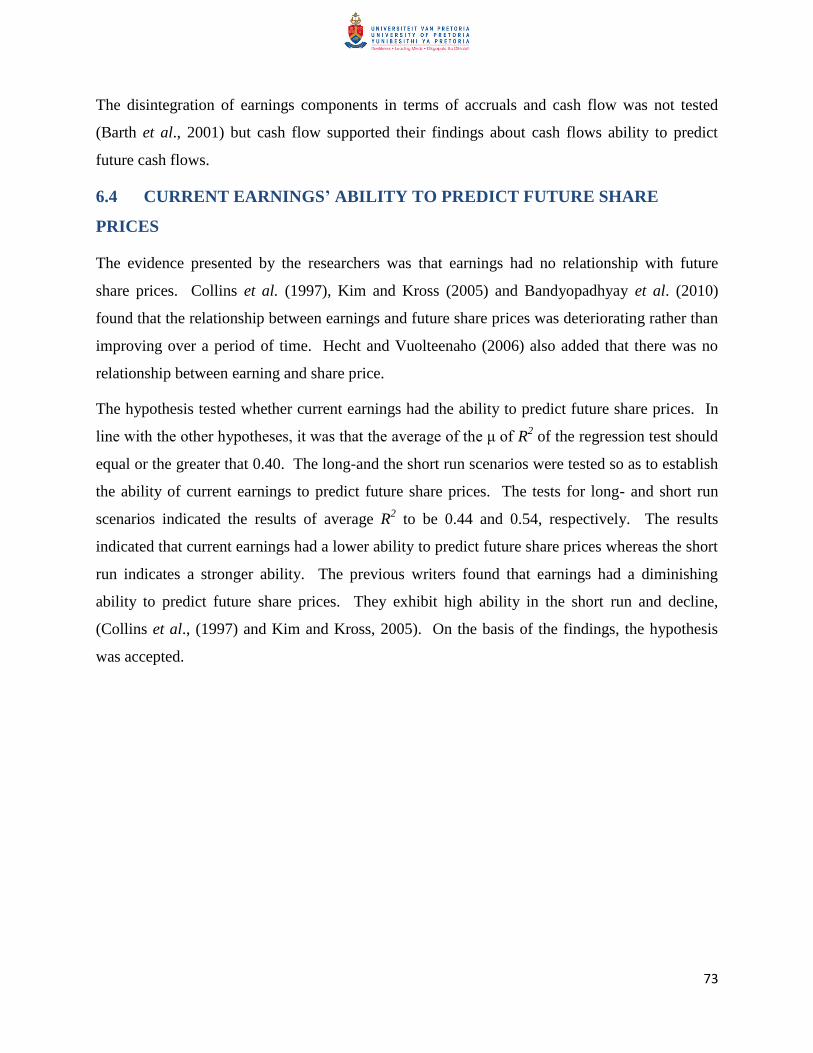
73
The disintegration of earnings components in terms of accruals and cash flow was not tested
(Barth et al., 2001) but cash flow supported their findings about cash flows ability to predict
future cash flows.
6.4 CURRENT EARNINGS’ ABILITY TO PREDICT FUTURE SHARE
PRICES
The evidence presented by the researchers was that earnings had no relationship with future
share prices. Collins et al. (1997), Kim and Kross (2005) and Bandyopadhyay et al. (2010)
found that the relationship between earnings and future share prices was deteriorating rather than
improving over a period of time. Hecht and Vuolteenaho (2006) also added that there was no
relationship between earning and share price.
The hypothesis tested whether current earnings had the ability to predict future share prices. In
line with the other hypotheses, it was that the average of the μ of R2 of the regression test should
equal or the greater that 0.40. The long-and the short run scenarios were tested so as to establish
the ability of current earnings to predict future share prices. The tests for long- and short run
scenarios indicated the results of average R2 to be 0.44 and 0.54, respectively. The results
indicated that current earnings had a lower ability to predict future share prices whereas the short
run indicates a stronger ability. The previous writers found that earnings had a diminishing
ability to predict future share prices. They exhibit high ability in the short run and decline,
(Collins et al., (1997) and Kim and Kross, 2005). On the basis of the findings, the hypothesis
was accepted.
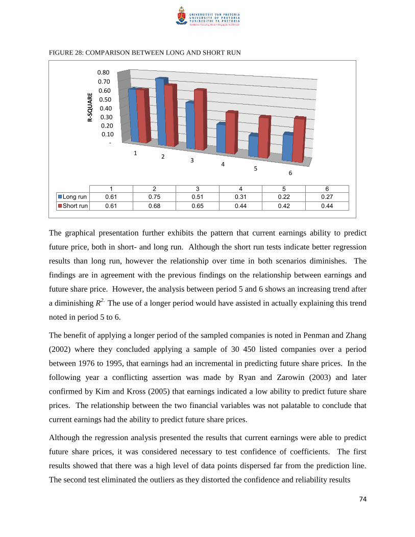
74
FIGURE 28: COMPARISON BETWEEN LONG AND SHORT RUN
The graphical presentation further exhibits the pattern that current earnings ability to predict
future price, both in short- and long run. Although the short run tests indicate better regression
results than long run, however the relationship over time in both scenarios diminishes. The
findings are in agreement with the previous findings on the relationship between earnings and
future share price. However, the analysis between period 5 and 6 shows an increasing trend after
a diminishing R2.
The use of a longer period would have assisted in actually explaining this trend
noted in period 5 to 6.
The benefit of applying a longer period of the sampled companies is noted in Penman and Zhang
(2002) where they concluded applying a sample of 30 450 listed companies over a period
between 1976 to 1995, that earnings had an incremental in predicting future share prices. In the
following year a conflicting assertion was made by Ryan and Zarowin (2003) and later
confirmed by Kim and Kross (2005) that earnings indicated a low ability to predict future share
prices. The relationship between the two financial variables was not palatable to conclude that
current earnings had the ability to predict future share prices.
Although the regression analysis presented the results that current earnings were able to predict
future share prices, it was considered necessary to test confidence of coefficients. The first
results showed that there was a high level of data points dispersed far from the prediction line.
The second test eliminated the outliers as they distorted the confidence and reliability results
- 0.10
0.20
0.30
0.40
0.50
0.60
0.70
0.80
12
34
56
R-S
QU
AR
E
1 2 3 4 5 6
Long run 0.61 0.75 0.51 0.31 0.22 0.27
Short run 0.61 0.68 0.65 0.44 0.42 0.44

75
The results improved, the R2 improved from 0.60 to 0.67 which symbolises a high level of
correlation. The t-test 0.3 in both tests augured well with the fact that they were below the 0.05
level of significance and the regression test was regarded as the one that presents higher ability
of current earnings to predict future share prices.
6.5 CURRENT CASH FLOWS’ ABILITY TO PREDICT FUTURE SHARE
PRICES
It is Charitou and Ketz (1990) who hold a strong view that share price is a reflection of
discounted future cash flows. Platt et al. (2010) questioned if the discounted future cash flows
were a reflection of the companies‘ values. An argument by Kaplan and Rubeck (1994) that
there was no evidence that suggested that discounted cash flows provided a reliable estimate for
the market value of share prices contrasted the view by Charitou and Ketz (1990).
It was also noted that some writers put string emphasis on accounting data as the strong predictor
of future share prices. DeFond and Huang (2002) and Choi and Sias (2012) emphasised that the
strong financial data suggested strong performance by the company and also persuasive to
conclude that the company will continue to produce such financial information. The viability of
the company is critical for investors to invest in the company. It is the same argument that was
presented by Higgins (2009) that investors look at how the company performed and project it
viability in the future. The sentiments were confirmed by Cohen and Kudryadstev (2012) that
investors look at the future prospects of the company based on the past experience and
knowledge about the historical market indices.
Another argument presented by the previous researchers suggested that investors react to the
market news (Cohen et al., 2002; Hecht and Vuolteenho (2006). All these factors have an
influence to the future share prices. The cash flow from operations form part of the accounting
data provided by companies, it could be well suggested that they have an impact on the future
prices of shares.

76
It was Kim and Kross (2005) who performed a regression analysis test between future share
price and current cash flow. They concluded that the contemporaneous relationship between
share price and current cash flow was declining. These tests were conducted over a period of 11
years. This was the only concrete evidence that was established where ability of current cash
flows to predict future share prices was tested.
It was felt that a further investigation be conducted on these financial variables. The hypothesis
was to prove that the μ average of future share prices will exceed R2 of 0.40. The outcome of the
tests was rejected as they concurred with Kim and Kross‘ (2005) findings. The averages of the
long run and short run were 0.24 and 0.33, respectively.
The findings showed a declining trend and only in the last two periods were some increases
started. The evidence is further presented graphically below:
FIGURE 29: COMPARISON BETWEEN LONG RUN AND SHORT RUN
The graph above shows a low relationship between current cash flows and future share prices.
The long run tests suggest that the R2 results started from a low base and kept on improving. At
period 6 they were at the same R2 of 0.40. The short term results graph indicate that the R2 for
the period were relatively higher that the long run graph although were below 0.40 with period 6
being and exception.
-
0.05
0.10
0.15
0.20
0.25
0.30
0.35
0.40
0.45
12
34
56
R-S
QU
AR
E
1 2 3 4 5 6
Long run 0.03 0.03 0.32 0.36 0.28 0.40
Short run 0.25 0.35 0.32 0.30 0.34 0.40
77
The short run showed a high level of erratic trend and no reliance could be placed on this
prediction model. The standard error average for both long run and short run results were 35.26
and 21.25, respectively/
The hypothesis was rejected and no further correlation of coefficient tests was performed. The
findings of this research project are in line with Kim and Kross (2005) that there was a low
relationship between current cash flows and future share price. The contrast was that Kim and
Kross (2005) found that the relationship was declining whereas the R2 results of this research
found that the relationship between current cash flows and future share prices was growing rather
than declining in the long run.
6.6 CONCLUSION
It was evident from the results and the discussions presented above that the results were not in
agreement with the previous researchers. The incidence opens up opportunities for further
researches to be undertaken. It was not expected of earnings to be able to predict future in a long
run. The reason for this assertion is the fact that most of the previous research findings have
concluded earnings are not good predictors of future share price particularly in a long run. The
results proved the opposite.
Again cash flows was able to predict future cash flows in a long run. The results or findings
defied the previous findings by the researcher who have provided evidence that current cash
flows were not good predictors of future cash flows in a long run.
It was noted that inability of current earnings to predict future cash flows was not expected.
There have been many writers who have provided and proved that current earnings had a high
predictive ability of future cash flows. Current flows inability to predict future share price was
expected as there has not been any findings that suggested otherwise.
Further key findings are discussed in chapter 7 below where possible further researches were
discussed in detail.

78

79
Chapter 7
Conclusion
This chapter discusses
80
7. CONCLUSION
The primary objective of this research was to establish the predictive ability of current earnings
and cash flows on future cash flows and share prices. In the earlier chapters it was established
that there was a relationship between the two elements, that is, earnings and cash flow from
operations. Earnings are useful in measuring company‘s annual performance generated from it
business operations. It is remembered that for the purposes of this study, EBITDA were used as
earnings as they are useful in measuring the true performance of a company performance. Cash
from operations represents cash that is actually generated by the company during the financial
period. It is clear that earnings measure financial performance whereas cash flow from
operations measure cash generated ability by business‘ operations.
It was then critical to assess whether their usefulness could be stretched beyond the mandatory
reporting as required by the Companies Act and IFRS to determine their ability to predict future
cash flows and future share prices. Investors have a propensity to invest in such businesses that
indicate such qualities, that is, ability to predict future growth in share prices and liquid enough
to pay dividends when due.
There were three objectives that we had set to achieve. The objectives that were set were
1. To investigate current earnings‘ ability to predict future cash flows;
2. To investigate current cash flows‘ ability to predict future cash flows;
3. To investigate which of the two variables, current earnings or cash flows had a better ability
to predict future share prices.
In achieving these objectives set above, a sample of 69 companies was selected from the JSE
listed companies. These companies excluded Mining, Financial Services and the companies that
did not have a completed set of financial data that included the period from 2001 to 2011. The
financial information was provided by McGregor BFA and downloaded into Excel worksheet.
The price data that coincided with financial year ends was obtained for measuring the
81
7.1 KEY FINDINGS
7.1.1 CURRENT EARNINGS ABILITY TO PREDICT FUTURE CASH FLOWS
The study found that current earnings could not predict future cash flows given that fact that cash
flow is one of the components of earnings (Barth et al., 2001). The findings proved that short and
the long run; earnings indicated a low relationship with future cash flows. The findings were
based on the regression analysis performed using Excel Data Analysis functions. The average R
square for earnings ability to predict future cash flows over a long run was R2=0.27. The average
was lower than expected. The short run test results provided that the R2 = 0.38. The hypothesis
had set the minimum of R2 = 0.40.
The previous researchers on the similar topics had found that there was a strong relationship
between current earnings and future cash flows. Dechow et al. (1998) and Kim and Kross
(2005) found that there was a strong relationship between these two variables. It came as
unexpected that the results will indicate that there was no strong relationship between the two
variables. As a result, the hypothesis was rejected and no further tests were conducted to verify
the possible outliers.
The results may suggest that a future study on the current earnings ability to predict future
earnings could be ensued to further investigate the discrepancy on the findings between these
findings and the previous researchers.
7.1.2 CURRENT CASH FLOWS’ ABILITY TO PREDICT FUTURE CASH FLOWS
However, current cash flows demonstrated that it had predictive ability on future cash flows.
Again this finding did not agree with the theory that was found earlier research reports. The
previous findings concluded that current cash flows had no predictive ability in a long run. In
this research, it was found that current cash flows did not only demonstrate the predictive ability
over future cash flows in a short run but also showed the power of predicting future cash flows
in the long run.
The R2 results in the short run and in the long run indicated R
2 = 0.43 and 0.46, respectively. The
findings were beyond the R2=0.40 threshold and they were subjected to further scrutiny through
the use of t-test of the confidence of coefficients.
82
The t-test results indicated quite a number of outliers. The outliers identified were eliminated
and a second round of confidence tests was conducted. The tests strengthened the earlier
findings that current cash flows had the ability to predict future cash flows.
It was rather unprecedented that current cash flows had a high ability to predict future cash flows
as shown in this research report. The study by Finger (1994) concluded that current cash flows
only had the ability to predict future cash flows only in a short run. These findings by Finger
(1994) were further supported by Dechow et al. (1998) and Kim and Kross (2005). It would
have also been interesting to assess the abilities of cash flows applying different forms of the
Statement of Cash flows to prove or disprove the findings by Orpurt and Zang (2007). The
findings of this research were limited to the Indirect Method.
7.1.3 CURRENT EARNINGS’ ABILITY TO PREDICT FUTURE SHARE PRICES
Current earnings were found have the ability to predict future share prices. The findings of this
research project defied the previous findings by Collins et al. (1997), Kim and Kross (2005) and
Bandyopadhyay et al. (2010) that earnings have a declining relationship with current earnings.
The previous findings went to allude that earnings were no a good predictor of future share
prices.
The findings were contrary to the previous researchers findings. Under normal strategic
financial management practices, earnings are capitalised, declared as dividends or reinvested
back to the company. The residual value impacts the earnings growth of the company which
subsequently impacts the balance sheet value of the shares. The combination of retained
earnings and shares issued is disclosed as shareholders‘ interest. In Collins et al. (1997) and Kim
and Kross (2005) the shareholders‘ interest is regarded as book values. The book values were
able to predict the future share prices. This shows that indirectly, earnings have the ability to
predict share price. The retained earnings or the book value are the value of the accounting share
price whereas, the share at the stock exchange could be perceived share prices by the capital
market. In the literature, it was note that between the accounting financial data and the capital
there is a lot of ―noise‖ that impact positively or adversely to the perception and the value of
share prices.
83
The hypothesis was accepted and the coefficients were subjected to a confidence test. The t-test
performed confirmed the earlier results that earnings do have the ability to predict future share
prices.
7.1.4 CURRENT CASH FLOWS’ ABILITY TO PREDICT FUTURE SHARE PRICES T
The findings tend to follow the assertion made by Charitou and Ketz (1990) that share prices
represented discounted future cash flows discount by a factor that took the riskiness other
economic cycles that impact the capital market. The results proved the previous literature to be
valid. The current cash flows could not predict future share prices. The tests were performed to
test the abilities of current cash flows with future share prices both in the long run and long run.
Kim and Kross (2005) conducted a similar test and obtained similar results.
The previous studies could not confirm the ability of current cash flows to predict future share
prices. Some writers argued that strong financial data, which include cash flows from
operations, had the ability to predict future share prices. Some pointed out that the past
experience and future expectations, influenced the value of the share prices. Again the economic
turbulences like inflation, recession or economic boom and interest rate influence the share
prices.
It is not easy to predict future cash share prices without factoring these factors into account. The
period between 2001 and 2011 has quite a number of incidences that impacted the economy and
somehow influence the markets. In 2001, America was attacked and the airline industry was
affected adversely and the global economy at large. This was followed by the financial crisis
which started in America and impacted the rest of the World. In South Africa, year June 2007,
the National Credit Act was implemented and followed by an economic meltdown which saw a
rise in interest rates and slowdown in retail activity. To highlight but a few issues, some of these
factors might have impacted the economy and capital market during the period of the research
report.
84
7.2 IMPLICATIONS TO STAKEHOLDERS
There are three stakeholders that are impacted by this research and its findings. These identified
stakeholders include the investors, traders and credit providers.
Investors
The investors normally take a long term view of their investment. Their decisions are influenced
amongst other things by the liquidity of the company and its ability to grow it future shares. The
study becomes important in making such decisions as they impact the future of the long term
investments. The study looked at both the long term and the short one to assess the future
predictability of these two elements. The results were mixed but provided the ―platform‖ for the
long term investors to apply in their investment decision making process..
Traders
The traders are looking mainly at the short term gains rather than the long term growth of the
shares. They are interested in short term gains resulting from the short term appreciation of the
share price and profit from such gains. The current earnings were able to predict future share
prices and this finding is important in their prediction tests.
Credit providers
Credit providers grant credit facilities to firms in a form of asset finance or loan funding and
other funding instruments. They are interested the firms‘ ability to meet its future obligation both
in the short run and in the near future. The research findings would influence the creditor
providers in terms of additional due diligence tests to perform in order to ascertain their ability to
predict the firm‘s cash flow generation ability.
85
7.3 POSSIBLE FUTURE RESEARCH
The possible future researches include the following:
The research could be repeated by taking a long term view of more than 11 years. It was
noticed that most of the findings the results tend to start at the high R2
then decline and in
the long run start to increase again. It would be interesting to the longer run impact of
these findings.
This study did not disintegrate the earnings elements in terms of accruals and cash flows
and to assess their impact of predictive ability on future cash flows. A multi regression
analysis would be highly recommended to perform this research.
The research focusing of the ability of current cash flow to predict future cash flows
applying two different forms of Statement of Cash flows. The research to find out which
of the two had a better ability to predict the future cash flows.
The study of predictive ability of current earnings and cash flows could be applied in
predicting other elements of financial information like earnings and dividend paying
abilities.
The predictive ability of other elements of the Statement of Cash flow, like Cash Utilised
in Investing or Financing activities would have on future earnings of the firms.
These five possible research would assist in adding knowledge of the abilities of financial
elements to predict future elements.
86
REFERENCES
Al‐Attar, A., & Hussain, S. (2004). Corporate data and future cash flows. Journal of Business Finance &
Accounting, 31(7‐8), 861-903.
Allen, M. F., & Cote, J. (2005). Creditors' use of operating cash flows: an experimental study. Journal of
Managerial Issues, 17(2), pp. 198-211.
Bali, T., Dermitas, O., & Tehranian, H. (2008). Aggregate earnings, firm-level earnings, and expected
stock returns. Journal of Financial and Quantitative Analysis, 43(3), 657-684
Bandyopadhyay, S. P., Chen, C., Huang, A. G., & Jha, R. (2010). Accounting conservatism and the
temporal trends in current earnings' ability to predict future cash flows versus future earnings:
evidence on the trade-off between relevance and reliability. Contemporary Accounting Research,
27(2), 413-460. doi: 10.1111/j.1911-3846.2010.01013.x
Banker, R. D., Huang, R., & Natarajan, R. (2009). Incentive contracting and value relevance of earnings
and cash flows. Journal of Accounting Research, 47(3), 647-678.
Barth, M. E., Cram, D. P., & Nelson, K. K. (2001). Accruals and the prediction of future cash flows. The
Accounting Review, 76(1), 27-58.
Billings, B. K., & Morton, R. M. (2001). Book-to-market components, future security returns, and errors
in expected future earnings. Journal of Accounting Research, 39(2), 197-219.
Bowen, R. M., Burgstahler, D., & Daley, L. A. (1986). Evidence on the relationships between earnings
and various measures of cash flow. Accounting Review, 61(4), 713-725.
Broome, O. W. (2004). Statement of cash flows: Time for change! Financial Analysts Journal, 60(2), pp.
16-22.
87
Charitou, A., & Ketz, J. E. (1990). Valuation of earnings, cash flows, and their components: An empirical
investigation. Journal of Accounting, Auditing & Finance, 5(4), 475-497.
Choi, N. Y., & Sias, R. W. (2012). Why does financial strength forecast stock returns? evidence from
subsequent demand by institutional investors. Review of Financial Studies, 25(5), 1550-1587.
Cohen, G., & Kudryavtsev, A. (2012). Investor rationality and financial decisions. Journal of Behavioral
Finance, 13(1), 11-16.
Cohen, R. B., Gompers, P. A., & Vuolteenaho, T. (2002). Who underreacts to cash-flow news? evidence
from trading between individuals and institutions. Journal of Financial Economics, 66(2-3), 409-
462.
Collins, D. W., Maydew, E. L., & Weiss, I. S. (1997). Changes in the value-relevance of earnings and
book values over the past forty years. Journal of Accounting and Economics, 24(1), 39-67.
Dechow, P. M., Kothari, S., & L Watts, R. (1998). The relation between earnings and cash flows. Journal
of Accounting and Economics, 25(2), 133-168.
DeFond, M. L., & Hung, M. (2003). An empirical analysis of analysts‘ cash flow forecasts. Journal of
Accounting and Economics, 35(1), 73-100.
Dontoh, A., Radhakrishnan, S., & Ronen, J. (2007). Is stock price a good measure for assessing value-
relevance of earnings? an empirical test. Review of Managerial Science, 1(1), 3-45.
Finger, C. A. (1994). The ability of earnings to predict future earnings and cash flow. Journal of
Accounting Research, 32(2), 210-223.
88
Givoly, D., & Hayn, C. (2000). The changing time-series properties of earnings, cash flows and accruals:
Has financial reporting become more conservative? Journal of Accounting and Economics, 29(3),
287-320.
Graham, M & Winfield, J. (2010). Financial statements: the essential guide to understanding and
interpreting the financial statements of a business. Cape Town: Cape business seminars
Gruca, T. S., & Rego, L. L. (2005). Customer satisfaction, cash flow, and shareholder value. Journal of
Marketing, 115-130.
Hecht, P., & Vuolteenaho, T. (2006). Explaining Returns with Cash-Flow Proxies. The Review of
Financial Studies, 19(1), 159-194
Higgins, R.C. (2009). Analysis for financial management. New York: McGraw Hill
International Financial Reporting Standards. (2010) A guide through IFRS. London: IFRS
Kaplan, S. N., & Ruback, R. S. (1995). The valuation of cash flow forecasts: An empirical analysis.
Journal of Finance, 50(4), 1059-1093.
Kim, M., & Kross, W. (2005). The ability of earnings to predict future operating cash flows has been
increasing—not decreasing. Journal of Accounting Research, 43(5), 753-780.
McGregor BFA , https://0-expert.mcgregorbfa.com.innopac.up.ac.za/. Retrieved 9 September 2012.
Metseeme, L. email [email protected]. Retrieved on 11 September 2012.
Murdoch, B., & Krause, P. (2012). The decline in matching and earnings‘ ability to forecast operating
cash flows. Journal of Applied Business Research (JABR), 28(4), 701-708.
89
Orpurt, S. F., & Zang, Y. (2007). Do direct cash flow disclosures help predict future operating cash flows
and earnings?
Platt, H., Demirkan, S., & Platt, M. (2010). Journal of Private equity, 13(4), 42-50
Penman, S. H., & Zhang, X. J. (2002). Accounting conservatism, the quality of earnings, and stock
returns. Accounting Review, 237-264.
Riedl, E. J. (2010). Discussion of 'accounting conservatism and the temporal trends in current earnings'
ability to predict future cash flows versus future earnings: Evidence on the trade-off between
relevance and reliability'. Contemporary Accounting Research, 27(2), 461-467. doi: 10.1111/j.1911-
3846.2010.01014.x
Roychowdhury, S. (2003). Management of Earnings through the Manipulation of Real Activities that
Affect Cash Flow from Operations,
Roychowdhury, S. (2006). Earnings management through real activities manipulation. Journal of
Accounting and Economics, 42(3), 335-370.
Ryan, S. G., & Zarowin, P. A. (2003). Why has the contemporaneous linear returns-earnings relation
declined? Accounting Review, 523-553.
Saunders, M., Lewis, P., & Thornhill, A. (2009). Research methods for business students. London:
Prentice Hill
Zikmund, W.G. (2003). Business research methods. Mason: South Western


![Estimating the Estimation of Accruals · Sloan [1996] finds that accrual earnings are less predictive of future earnings than cash earnings (i.e. accruals earnings are less persistent](https://img.dokumen.tips/doc/110x75/5e692fec32f2f67ce035a065/estimating-the-estimation-of-accruals-sloan-1996-finds-that-accrual-earnings-are.jpg)


