Embed Size (px)
Citation preview

Civil Engineering Infrastructures Journal, 48(2): 271-283, December 2015
ISSN: 2322-2093
271
Prediction of Permanent Earthquake-Induced Deformation in Earth Dams
and Embankments Using Artificial Neural Networks
Barkhordari Bafghi, K.1*
and Entezari Zarch, H.2
1 Assistant professor, Department of Civil Engineering, Yazd University, Yazd, Iran.
2 M.Sc. Student, Department of Civil Engineering, Yazd University, Yazd, Iran.
Received: 14 Apr. 2014 Revised: 11 Jan. 2015 Accepted: 10 Mar. 2015
Abstract: This research intends to develop a method based on the Artificial Neural Network (ANN) to predict permanent earthquake-induced deformation of the earth dams and embankments. For this purpose, data sets of observations from 152 published case histories on the performance of the earth dams and embankments, during the past earthquakes, was used. In order to predict earthquake-induced deformation of the earth dams and embankments a Multi-Layer Perceptron (MLP) analysis was used. A four-layer, feed-forward, back-propagation neural network, with a topology of 7-9-7-1 was found to be optimum. The results showed that an appropriately trained neural network could reliably predict permanent earthquake-induced deformation of the earth dams and embankments.
Keywords: Artificial neural networks, Earth dam, Earth embankment, Earthquake-induced deformation.
INTRODUCTION
The seismic performance of slopes and
earth structures is often assessed by
calculating the permanent down slope
sliding deformation expected during
earthquake shaking. Newmark (1965) first
proposed a rigid sliding block procedure
and this procedure is still the basis of many
analytical techniques used to evaluate the
stability of slopes during earthquakes.
Over the last few years, Artificial
Neural Networks (ANNs) have been used
successfully for modeling almost all
aspects of geotechnical engineering
problems. The literature reveals that ANNs
have been extensively used for predicting
axial and lateral load capacities in the
compression and uplift of pile foundations
(Shahin, 2008; Das and Basudhar, 2006),
*corresponding author Email: [email protected]
dams (Behnia et al., 2013; Miao et al.,
2013; Mohammadi et al., 2013; Marandi et
al., 2012; Mata, 2011; Tsompanakis et al.,
2009; Kim and Kim, 2008) and slope
stability (Erzin and Cetin, 2012; Zhao,
2008; Ferentinou and Sakellariou, 2007).
Other applications of ANNs in
geotechnical engineering include
Liquefaction during earthquakes (Hanna et
al., 2007; Javadi et al., 2006; Baziar and
Ghorbani, 2005) tunnels, and underground
openings (Mahdevari and Torabi, 2012;
Gholamnejad and Tayarani, 2010; Yoo and
Kim, 2007).
In this article, with respect to successful
modeling the geotechnical engineering
problems with ANN method most of the
aspects of geotechnical engineering
measurements of earthquake-induced
deformation, which are recorded in
different earth dams and embankments,
have been reviewed and analyzed. For this
purpose, data sets of observations from

Barkhordari Bafghi, K. and Entezari Zarch, H.
272
152 published case histories on the
performance of the earth dams and
embankments during the past earthquakes
have been used. The data from these case
studies have been used to train and test the
developed neural network model, to enable
the prediction of the magnitude of
earthquake-induced deformation of the
earth dams and embankments.
PERMANENT EARTHQUAKE-
INDUCED DEFORMATION OF THE
EARTH EMBANKMENTS
Newmark (1965) proposed that the seismic
stability of slopes would be assessed in
terms of earthquake-induced deformations,
as this criterion ultimately governs the
serviceability of the earth structure after
the earthquake. Newmark surmised that
the factor-of-safety of a slope would vary
with time as the destabilizing inertial
forces imposed on the slope varied
throughout the duration of earthquake
shaking. When the inertial forces acting on
a failure mass are large enough to exceed
the available resisting forces, the factor-of-
safety of the slope would fall below one,
thereby initiating an episode of permanent
down slope displacement. Newmark
formulated this concept by making an
analogy that an earth mass sliding over a
shear surface could be modeled as a block
sliding along an inclined plane.
The sliding-block analogy proposed by
Newmark has provided the conceptual
framework from which all deformation-
based methods are derived. Today, a suite
of roughly 30 different deformation-based
methods are available to practitioners and
researchers for evaluating the seismic
slope stability of earth structures and
embankments. These methods are the
result of roughly 50 years of research
focused on method development and
refinement.
On a conceptual level, all deformation-
based methods are models-simplified
approximations of the real physical
mechanism of seismic-induced
deformation in the slopes. There are three
fundamental models that all deformation-
based methods are based on. These model
categories range from simple to complex
and differ with respect to the assumptions
and idealizations used to represent the
mechanism of earthquake-induced
deformation, these are:
1. Rigid-block models. The rigid-block
model was originally proposed by Newmark
(1965) and is based on the sliding-block
analogy. To briefly reiterate, the potential
landslide block is modeled as a rigid mass
that slides in a perfectly plastic manner on an
inclined plane. The mass experiences no
permanent displacement until the base
acceleration exceeds the critical acceleration
of the block, at which time the block begins
to move down the slope displacements are
calculated by integrating the parts of an
acceleration-time history that lie above the
critical acceleration to determine a velocity-
time history. The velocity-time history is
then integrated to yield the cumulative
displacement. Sliding continues until the
relative velocity between the block and base
reaches zero. Since 1965, many researchers
such as Newmark (1965), Sarma (1975),
Jibson (2007), and Bray and Travasarou
(2007) have developed graphs and relations
for calculating earthquake-induced
deformation, based on the rigid-block model.
2. Decoupled models. Soon after
Newmark published his rigid-block
method, more sophisticated analyses were
developed to account for the fact that
landslide masses are not rigid bodies, but
deform internally when subjected to
seismic shaking. The most commonly used
among these analyses has been developed
by Makdisi and Seed (1978), Hynes-
Griffin, and Franklin (1984). A rigorous
decoupled analysis estimates the effect of a
dynamic response on permanent sliding in
a two-step procedure: a) A dynamic-
response analysis of the slope, assuming

Civil Engineering Infrastructures Journal, 48(2): 271-283, December 2015
273
no failure surface, is performed using
programs such as QUAD4M or SHAKE.
By estimating the acceleration-time
histories at several points within the slope,
an average acceleration-time history for
the slope mass above the potential failure
surface is developed. b) The resulting time
history of the previous step is used as input
data into a rigid-block analysis, and the
permanent displacement is estimated. This
approach is referred to as a decoupled
analysis because the computation of the
dynamic response and the plastic
displacement are performed independently.
3. Coupled models. In a fully coupled
analysis, the dynamic response of the sliding
mass and the permanent displacement are
modeled together, such that, the effect of
plastic sliding displacement on the ground
motion is taken into account. The most
commonly used of such analyses has been
developed by Bray and Travasarou (2007).
As mentioned, the most commonly
available methods for evaluating the
permanent earthquake-induced deformation
of the earth embankments are based on the
sliding-block analogy proposed by Newmark,
but there has been some concern expressed
by others that the Newmark method may not
model the crest settlement caused by the
earthquake accurately. Day (2002)
demonstrated that it is theoretically possible
for dry granular slopes to settle and spread
laterally without earthquake accelerations
exceeding the yield values to initiate the
slides. He states that the Newmark method
may prove to be unreliable in some instances.
Matsumoto (2002) described centrifuge shake
table tests, with supporting nonlinear analyses
for modeled accelerations up to 0.7g, which
revealed only shallow raveling with no deep
shear surfaces in the core zones and no
definite slip surfaces anywhere in the rockfill
dam models. Accordingly, he states that the
hypothesis of deep slide surfaces in the
Newmark approach “may be somewhat
erroneous”.
Swaisgood and Au-Yeung (1991), after
reviewing many photos of earthquake
damages to dams, disclosed that crest
settlements and deformations (for
structures not subject to liquefaction) seem
to be from slumping and spreading
movements that occur within the dam
body, without distinct signs of shearing
displacement. This appears to be true for
earthfill embankments as well as rockfill
dams.
Accordingly, Swaisgood (2003) studied
69 published case histories on the
performance of earth dams and embankments
during the past earthquakes and developed a
mathematical relationship between the crest
settlement and the three factors, peak
horizontal ground acceleration (PGA),
earthquake magnitude (M) and dam height
(H). Singh et al. (2007), by comparing
permanent deformations estimated from some
Newmark methods with observations from
122 published case histories on performance
of earth dams and embankments during past
earthquakes, indicated that the estimated
permanent earthquake-induced deformations
were, in general, smaller than the observed
deformations. Singh et al. developed a
relationship among permanent earthquake-
induced deformations, the ratio of yield
acceleration (Ky), and the peak horizontal
ground acceleration (PGA) based on
observational data.
ARTIFICIAL NEURAL NETWORK
An ANN model is a mathematical or
computational model that is inspired by the
structure and/or functional aspects of
biological neural networks and is in fact an
emulation of the biological neural system.
Neural network analysis can be used to
handle non-linear problems that are not
well-suited to be handled by the classical
analysis methods (Erzin and Cetin, 2012).
ANN includes two working phases, the
phase of learning and that of recall. During
the learning phase, known data sets are
commonly used as a training signal in the

Barkhordari Bafghi, K. and Entezari Zarch, H.
274
input and output layers. The recall phase is
performed by one pass using the weight
obtained in the learning phase (Mahdevari
and Torabi, 2012).
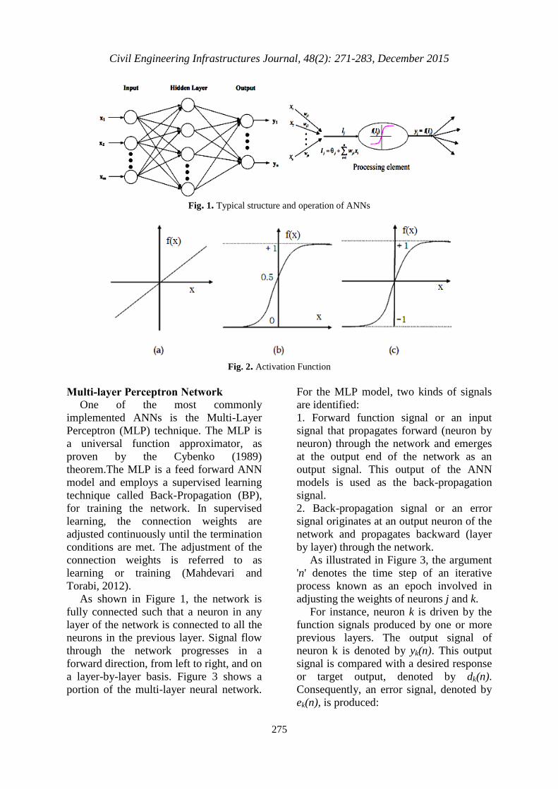
Artificial Neural Networks consist of a
number of artificial neurons variously
known as processing elements (PEs)
“nodes” or “units”. For multilayer
perceptrons (MLPs), which are the most
commonly used ANNs in geotechnical
engineering, the processing elements are
usually arranged in layers: An input layer,
an output layer, and one or more
intermediate layers called hidden layers
(Figure 1).
Each processing element in a specific
layer is fully or partially connected to many
other processing elements via weighted
connections. The scalar weights determine
the strength of the connections between the
interconnected neurons. A zero weight
refers to no connection between two
neurons and a negative weight refers to a
prohibitive relationship. From many other
processing elements, an individual
processing element receives its weighted
inputs, which are summed and a bias unit or
threshold is added or subtracted. The bias
unit is used to scale the input to a useful
range to improve the convergence properties
of the neural network. The result of this
combined summation is passed through a
transfer function to produce the output of
the processing element (For node j, this
process is summarized in Eqs. (1) and (2)
and illustrated in Figure 1) (Shahin et al.,
2008).
1
n
j j ji iiI w x
(1)
( )i jy f I
(2)
where 𝐼𝑗: is the activation level of node
j; 𝑤𝑗𝑖: is the connection weight between
nodes j and i; 𝑥𝑖: is the input from node i,
i,…, 1, 0= n; θj: is the bias or threshold for
node j; 𝑦𝑖: is the output of node j and f).(: is
the transfer function.
The transfer functions are designed to
map a neuron or layer-net output to its
actual output. The type of these transfer
functions depends on the purpose of the
neural network. Linear (PURELIN) and
Nonlinear (LOGSIG, TANSIG) functions
can be used as transfer functions (Figure
2). As is known, a linear function satisfies
the superposition concept. The function is
shown in Figure 2a. The mathematical
equation for the linear function can be
written as:
.y f x x (3)
where α: is the slope of the linear function.
As shown in Figure 2b, sigmoidal (S shape)
function is the most common nonlinear type
of the activation used to construct the neural
networks. It is mathematically well-behaved,
differentiable, and a strictly increasing
function. A sigmoidal transfer function can
be written in Eq. (4).
1
,0 ( ) 11 cx
f x f xe
(4)
where c: is the shape parameter of the
sigmoid function. Which c is a constant
that typically varies between 0.01 and
1.00. By varying this parameter, different
shapes of the function can be obtained as
illustrated in Figure 2b; x: is the weighted
sum of the inputs for a processing unit.
This function is continuous and
differentiable. Tangent sigmoidal function
is described by the following mathematical
form (Figure 2c) (Park, 2011):
2
1, 1 11 cx
f x f xe
(5)
Civil Engineering Infrastructures Journal, 48(2): 271-283, December 2015
275
Fig. 1. Typical structure and operation of ANNs
Fig. 2. Activation Function
Multi-layer Perceptron Network
One of the most commonly
implemented ANNs is the Multi-Layer
Perceptron (MLP) technique. The MLP is
a universal function approximator, as
proven by the Cybenko (1989)
theorem.The MLP is a feed forward ANN
model and employs a supervised learning
technique called Back-Propagation (BP),
for training the network. In supervised
learning, the connection weights are
adjusted continuously until the termination
conditions are met. The adjustment of the
connection weights is referred to as
learning or training (Mahdevari and
Torabi, 2012).
As shown in Figure 1, the network is
fully connected such that a neuron in any
layer of the network is connected to all the
neurons in the previous layer. Signal flow
through the network progresses in a
forward direction, from left to right, and on
a layer-by-layer basis. Figure 3 shows a
portion of the multi-layer neural network.
For the MLP model, two kinds of signals
are identified:
1. Forward function signal or an input
signal that propagates forward (neuron by
neuron) through the network and emerges
at the output end of the network as an
output signal. This output of the ANN
models is used as the back-propagation
signal.
2. Back-propagation signal or an error
signal originates at an output neuron of the
network and propagates backward (layer
by layer) through the network.
As illustrated in Figure 3, the argument
'n' denotes the time step of an iterative
process known as an epoch involved in
adjusting the weights of neurons j and k.
For instance, neuron k is driven by the
function signals produced by one or more
previous layers. The output signal of
neuron k is denoted by yk(n). This output
signal is compared with a desired response
or target output, denoted by dk(n).
Consequently, an error signal, denoted by
ek(n), is produced:

Barkhordari Bafghi, K. and Entezari Zarch, H.
276
k k ke n d y n (6)
The error signal is then propagated back
to adjust the weights and bias levels of
each layer. A neural network learns about
the relationships between the input and
output data through this iterative process.
Ideally, the network becomes more
knowledgeable about relationships after
each iteration or the epoch of the learning
process, by using the back-propagation or
error back-propagation algorithm (Hertz et
al., 1991; Rumelhart et al., 1986).
Artificial Neural Networks for Predicting
Permanent Earthquake-Induced
Deformation of Earth Embankments
Network Architecture Generally, there is no direction or a
precise method for determining the most
appropriate number of neurons that need to
be included in each hidden layer in the
neural networks. This problem becomes
more complicated as the number of hidden
layers in the network increases. The
concept of the neural networks appears to
indicate that increasing the number of
hidden neurons provides a greater potential
for developing a solution that maps or fits
the training patterns closely, as they
increase the number of possible function
calculations. However, a large number of
hidden neurons can lead to a solution,
which, while mapping the training points
closely, deviates dramatically from the
optimum trend. Although, the network can
provide almost perfect answers to the set
of problems with which it was trained, it
may fail to produce meaningful answers to
other ‘‘new’’ problems. This is a result of
‘overfitting’. Overfitting problem or poor
generalization capability occurs when a
neural network over learns during the
training period. As a result, ‘a too well-
trained model’ may not perform well in an
unseen data set, on account of its lack of
generalization capability. Several
approaches have been suggested in
literature to overcome this problem. The
first method is an early learning stopping
mechanism in which the training process is
concluded as soon as the overtraining
signal appears. The signal can be observed
when the prediction accuracy of the trained
network applied to a test set gets worsened
at that stage of the training period, when it
gets worsened. The second approach is the
Bayesian Regularization. This approach
minimizes the overfitting problem by
taking into account the goodness-of-fit as
well as the network architecture. The early
stopping approach requires the data set to
be divided into three subsets: Training,
test, and verification sets. The training and
the verification sets are the norm in all
model training processes. The test set is
used to test the trend of the prediction
accuracy of the model trained at some
stages of the training process. At much
later stages of the training process, the
prediction accuracy of the model may start
worsening for the test set. This is the stage
when the model should cease to be trained
to overcome the over-fitting problem
(Park, 2011). Furthermore, a large number
of hidden neurons slow down the operation
of the network.
Most Feed-forward Back-Propagation
Neural Networks use one or two hidden
layers. In order to obtain a good
performance of the ANN, tuning of the
ANN architecture and parameters is
essential (Mahdevari and Torabi, 2012). In
our case, the ANN architecture has been
tested with various numbers of hidden
layers and nodes per hidden layers, and the
ANN parameters are checked with various
transformation functions to find better
values and architecture. The transformation
functions used are purelin, logistic sigmoid
(logsig), and the hyperbolic tangent sigmoid
(tansig) function.
Input Parameters An important step in developing ANN
models is to select the model input
variables that have the most significant

Civil Engineering Infrastructures Journal, 48(2): 271-283, December 2015
277
impact on model performance. A good
subset of input variables can substantially
improve model performance.
It is difficult to determine all the relevant
parameters that influence the prediction of
earthquake-induced deformation of earth
embankments. The selected parameters
affecting earthquake-induced deformation
of earth dams and embankments, used in
this study were: Dam type, dam height (H),
magnitude of the earthquake (MW), peak
ground acceleration (PGA), predominant
period of the earthquake ground motion
(TP), fundamental (elastic) period of the
earth structure (TD), and yield acceleration
(Ky).
Data Preparation Before training and implementing, the
data set was divided randomly into training,
validation, and test subsets. In the present
study, the data sets of observations from 152
published case histories on the performance
of earth dams and embankments during the
past earthquakes were collected. Some of
these data are given in Table 1.
From these, 70% of the data were
chosen for training, 15% for validation,
and 15% for the final test. The training set
was used to generate the model and the
validation set was used to check the
generalization capability of the model.
Once the available data have been
divided into their subsets (i.e., training,
testing, and validation), it is important to
pre-process the data in a suitable form
before applying them to the ANN. Data
pre-processing is necessary to ensure that
all variables receive equal attention during
the training process (Maier and Dandy,
2000). Moreover, pre-processing usually
speeds up the learning process. Pre-
processing can be in the form of data
scaling, normalization, and transformation
(Masters, 1993).
In this study the input and output data
were scaled to lie between 0 and 1, by
using Eq. (7).
min
max min
( )
( )norm
x xx
x x
(7)
where xnorm: is the normalized value, x: is
the actual value, xmax: is the maximum
value and xmin: is the minimum value.
Fig. 3. Signal-flow schematic diagram of back-propagation neural networks

Barkhordari Bafghi, K. and Entezari Zarch, H.
278
Table 1. Some of case history
∆ (m) TD (s), ay (w/o and
with vert. accn) (g)
Earthquake: Date, Mw, amax (g),
Dist. (km), Tp (s) Dam, type, height (m)
0.0410 1.08, 0.34, 0.24 10/17/89, 7.0, 0.26, 16, 0.32 Anderson, 8, 73.2
0.0140 1.08, 0.27, 0.20 4/24/84, 6.2, 0.41, 16, 0.32 Anderson, 8, 71.6
0.6000 0.08, 0.28, 0.21 10/17/89, 7.1, 0.33, 27, 0.32 Artichoke, 2, 4.0
0.7890 0.79, 0.21, 0.17 10/17/89, 7.0, 0.58, 11, 0.32 Austrian, 7, 21.5
0.7000 0.53, 0.08, 0.07 10/23/04, 6.8, 0.12, 24, 0.32 Asagawara regulatory, 7, 56.4
2.5000 0.89, 0.06, 0.06 7/28/76, 7.8, 0.20, 150, 0.52 Baihe, 7, 66.0
0.0010 0.54, 0.16, 0.14 7/21/52, 7.3, 0.12, 74, 0.40 Bouquet Canyon, 5, 62.0
0.0010 0.76, 0.25, 0.17 1/17/94, 6.9, 0.19, 67, 0.45 Brea, 7, 27.4
0.6000 0.45, 0.16, 0.13 7/21/52, 7.3, 0.30, 32, 0.32 Buena Vista, 5, 6.0
0.4500 0.99, 0.12, 0.11 4/18/06, 8.3, 0.57, 32, 0.32 Chabbot, 5, 43.3
0.0010 0.99, 0.12, 0.11 10/17/89, 7.0, 0.10, 60, 0. Chabbot, 5, 43.3
2.6400 0.25, 0.05, 0.05 1/26/01, 7.6, 0.50, 13, 0.32 Chang, 7, 15.5
0.0700 0.38, 0.09, 0.08 10/23/04, 6.8, 0.10, 21, 0.32 Chofukuji, 7, 27.2
3.8700 0.11, 0.01, 0.01 12/17/87, 6.7, 0.12, 40, 0.32 Chonan, 4, 6.1
0.3500 0.83, 0.28, 0.23 4/4/43, 7.9, 0.19, 89, 0.60 Cogoti D/S, 9, 85.0
0.0010 0.24, 0.28, 0.83 3/28/65, 153, 0.04, 7, 1, 0.55 CogotiD/S, 9, 85.0
0.0010 0.83, 0.28, 0.24 7/8/75, 7.5, 7, 0.05, 165, 0.57 CogotiD/S, 9, 85.0
0.0010 0.83, 0.28, 0.24 3/8/85, 7.7, 0.03, 280, 0.96 CogotiD/S, 9, 85.0
0.0010 0.69, 0.13, 0.11 10/1/87, 0, 6, 0,06, 29, 0.25 Cogswell 9, 85.0
0.0160 0.69, 0.15, 0.14 6/28/91, 5.6, 0.26, 4, 0.25 Cogswell 9, 85.0
0.0500 0.23, 0.26, 0.24 1/26/01, 7.6, 0.20, 90, 0.55 Demi 1, 7, 17.0
1,6400 0.22, 0.34, 0.24 7/8/76, 7.8, 0.90, 20, 0.30 Douhe 4, 16.0
0.0300 0.65, 0.12, 0.10 7/21/52, 7.3, 0.12, 72, 0.28 DryCanyon 5, 22.0
32.000 0.49, 0.00, 0.00 3/28/65, 7.2, 0.80, 40, 0.32 ElCobre 12, 32.5
0.0460 1.58, 0.55, 0.39 3/14/79, 7.6, 0.23, 110, 0.55 ElInfiernilloD/S 8, 148.0
0.0400 1.58, 0.08, 0.08 10/11/75, 5.9, 0.08, 79, 0.34 ElInfiernilloU/S 8, 46.0
0.0200 1.58, 0.09, 0.08 11/15/75, 7.5, 0.09, 23, 0.32 ElInfiernilloU/S 8, 146.0
0.1280 1.58, 0.19, 0.18 3/14/79, 7.6, 0.23, 110, 0.55 ElInfiernilloU/S 8, 148.0
0.0600 1.58, 0.05, 0.03 10/25/81, 7.3, 0.05, 81, 0.34 ElInfiernilloU/S 8, 146.0
0.1100 1.58, 0.11, 0.10 9/19/85, 8.1, 0.13, 76, 0.53 ElInfiernilloU/S 8, 146.0
(1): Dam types: 1: 1-zone levee, 2: Multi zone levee, 3: 1-zone earth dam, 4: 1-zone embankment, 5: 1-zone hydraulic fill
dam; 6: Multi-zone hydraulic fill; 7: Compacted multi-zone dam; 8: Multi-zone rockfill dam; 9: Concrete-Faced rockfill Dam
(CFRD); 10: Concrete-faced decomposed granite or gravel dam; 11: Natural slope; 12: Upstream constructed tailings dam;
13: Downstream constructed tailings dam.
Training of the Network In a supervised BP training, the
connection weights are adjusted
continuously until termination conditions are
met. The adjustment of the connection
weights is referred to as learning or training
(Pezeshk et al., 1996). The back-propagation
learning algorithm has been applied with
great success to model many phenomena in
the field of geotechnical engineering (Shahin
et al., 2001). Several training algorithms of
back-propagation have been developed (for
example; Gradient descent and Levenberg-
Marquardt) (Mohammadi and Mirabedini,
2014). In this study the Levenberg-
Marquardt back-propagation algorithm was
chosen for training the ANNs, because it is
known to be the fastest method for training
moderate-sized feed-forward neural
networks. The resulting target network
should produce a minimum error for the
training pattern and give a generalized

Civil Engineering Infrastructures Journal, 48(2): 271-283, December 2015
279
solution that performs well with the testing
pattern. It has lower memory requirements
than most algorithms and usually reaches an
acceptable error level quite rapidly, although
it can then become very slow in converging
properly on an error minimum (Erzin and
Cetin, 2013).
Validation and Testing the ANN Model Once the training phase of the model has
been successfully accomplished, the
performance of the trained model should be
validated. The purpose of the model
validation phase is to ensure that the model
has the ability to generalize within the limits
set by the training data in a robust fashion,
rather than simply having memorized the
input-output relationships that are contained
in the training data.
Testing and validation of the ANN
model was done with new data sets. These
data were not previously used while
training the network.
The Mean Squared Error (MSE) and
coefficient of correlation factor (R)
between the predicted and measured values
were taken as the performance measures.
The MSE was calculated as:
21( )
Q
MSE d oQ
(8)
where d, o, and Q: represent the target
output, the output, and the number of
input-output data pairs, respectively.
RESULTS AND DISCUSSION
As there is no direct, precise way of
determining the most appropriate number
of hidden layers and number of neurons in
each hidden layer, a trial and error
procedure is typically used to identify the
best network for a particular problem
(Gholamnejad and Tayarani, 2010). After
building several MLP models based on
trial and error, the best results of each
model, listed in Table 2, are compared and
the one with the maximum correlation
factor (R) and minimum Mean Squared
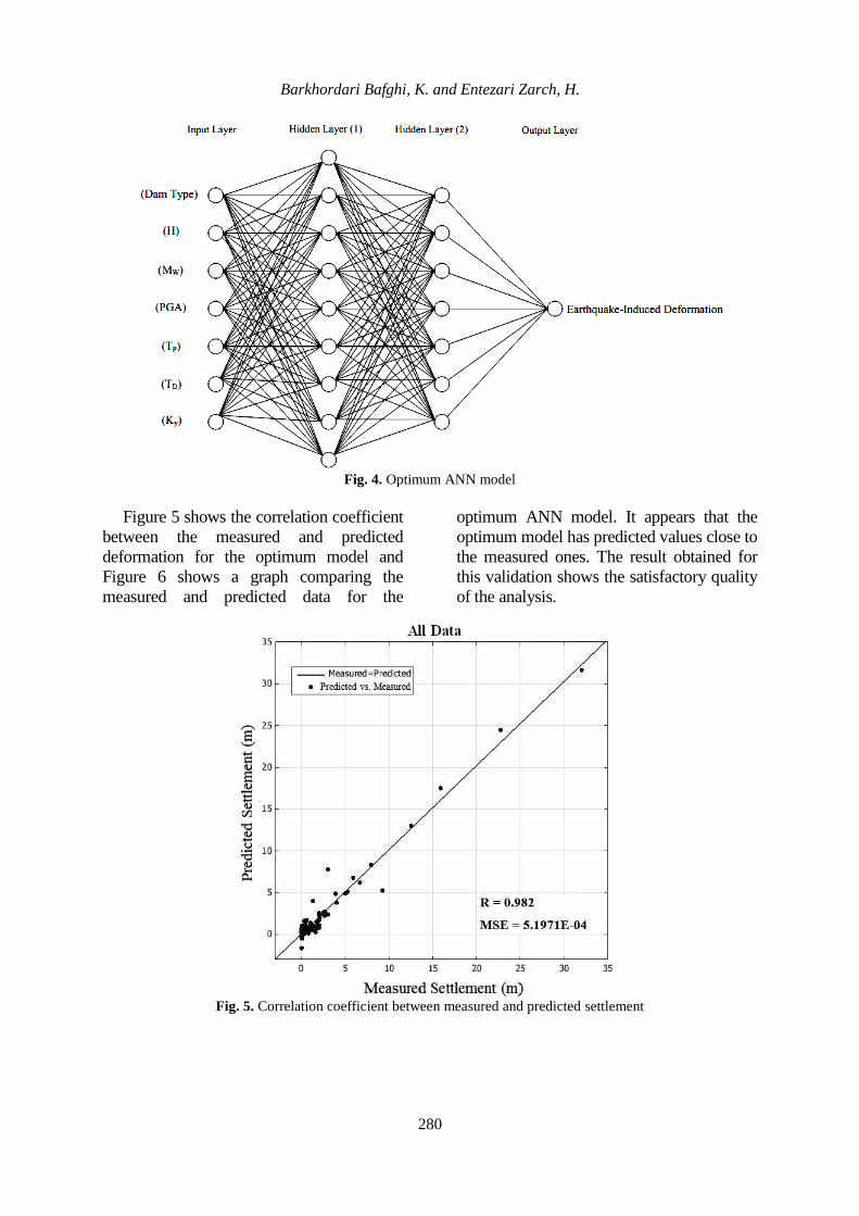
Error (MSE) is chosen. Therefore, based
on these criteria, the optimum ANN
architecture was found to be a four-layer,
feed-forward, back-propagation neural
network with a topology of 7-9-7-1. This
ANN architecture is shown in Figure 4. As
shown in Table 2, for optimum ANN
architecture, the correlation factor and
minimum of Mean Squared Error are
1.600E-03 and 0.982, respectively.
Table 2. Performance of the neural network models
No. Model architecture Transfer function MSE (training) MSE (validation) MSE (test) R (All)
1 7-10-1 logsig-purelin 2.700E-03 1.700E-03 2.400E-03 0.910
2 7-12-1 logsig-purelin 1.869E-04 2.110E-02 1.360E-02 0.823
3 7-10-1 tansig-purelin 1.700E-03 5.345E-04 1.900E-03 0.943
4 7-12-1 tansig-purelin 1.422E-04 5.100E-03 3.600E-03 0.948
5 7-7-5-1 logsig-logsig-purelin 1.449E-04 5.200E-03 1.800E-02 0.883
6 7-9-7-1 logsig-logsig-purelin 1.941E-04 9.652E-04 1.600E-03 0.982
7 7-11-7-1 logsig-logsig-purelin 1.225E-04 4.394E-04 3.145E-03 0.977
8 7-13-7-1 logsig-logsig-purelin 2.519E-04 6.195E-04 2.839E-03 0.976
9 7-7-5-1 tansig-tansig-purelin 4.700E-03 5.700E-03 1.190E-02 0.822
10 7-9-7-1 tansig-tansig-purelin 2.500E-03 1.800E-03 7.470E-04 0.924
11 7-7-5-1 logsig-tansig-purelin 7.721E-04 6.000E-03 1.700E-03 0.935
12 7-9-7-1 logsig-tansig-purelin 6.654E-05 1.800E-03 5.100E-03 0.965
13 7-9-7-1 tansig-logsig-purelin 2.490E-04 1.100E-03 6.100E-03 0.956
14 7-11-7-1 tansig-logsig-purelin 1.286E-03 4.257E-03 1.628E-03 0.936
Barkhordari Bafghi, K. and Entezari Zarch, H.
280
Fig. 4. Optimum ANN model
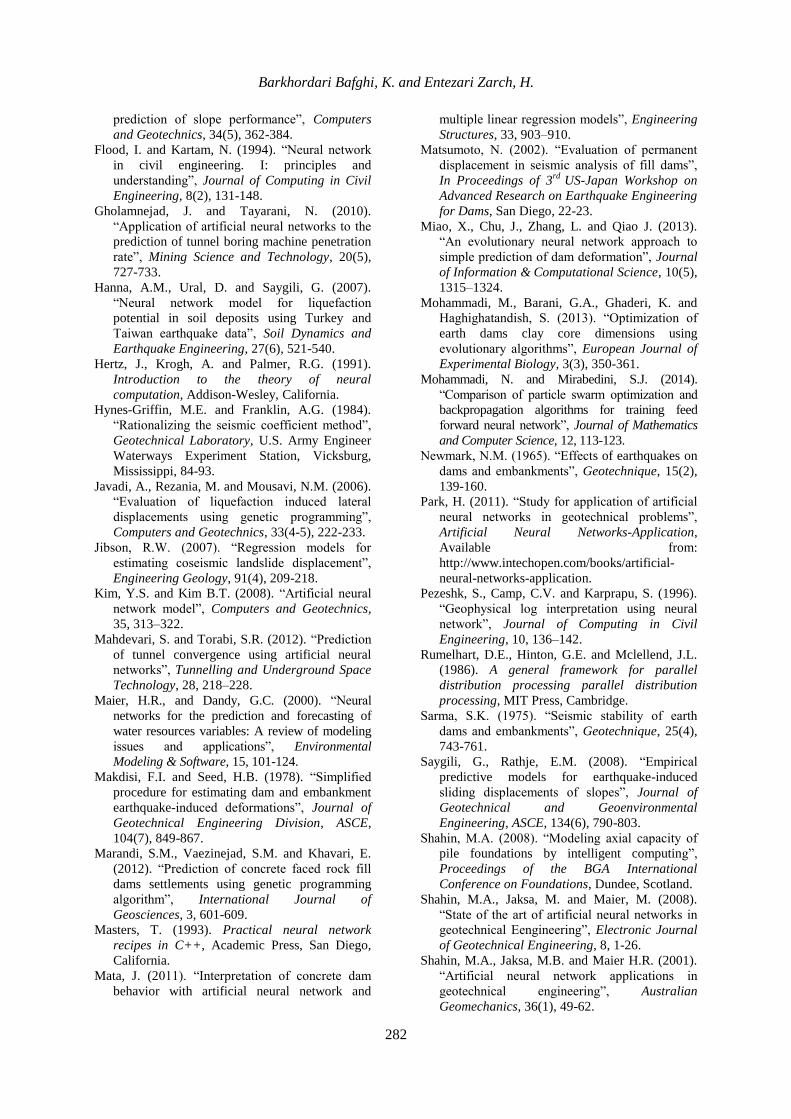
Figure 5 shows the correlation coefficient
between the measured and predicted
deformation for the optimum model and
Figure 6 shows a graph comparing the
measured and predicted data for the
optimum ANN model. It appears that the
optimum model has predicted values close to
the measured ones. The result obtained for
this validation shows the satisfactory quality
of the analysis.
Fig. 5. Correlation coefficient between measured and predicted settlement

Civil Engineering Infrastructures Journal, 48(2): 271-283, December 2015
281
Fig. 6. Comparison between measured and predicted settlement
CONCLUSIONS
This study investigated the potential of
artificial neural networks (ANN) for
predicting earthquake-induced deformation
of earth dams and embankments. It was
found that the feed-forward back-
propagation neural network models
successfully learned from the training
samples in a manner in which their outputs
converged to values very close to the
desired outputs. However, the relationship
among the inputs and outputs is very
complex. The results obtained are still
highly encouraging and satisfactory. The
optimum ANN architecture was found to
have seven neurons in the input layer, nine
and seven neurons in two hidden layers,
and one neuron in the output layer (7-9-7-
1). As a neural network can update “its”
knowledge over time, if more training data
sets are processed, the neural networks will
result in greater accuracy and more robust
prediction than any other analysis
technique. With regard to the fact that the
accuracy of the proposed ANN model is
reasonably high, this model can be used to
predict earthquake-induced deformation of
earth embankments.
REFERENCES
Baziar, M.H. and Ghorbani, A. (2005). “Evaluation
of lateral spreading using artificial neural
networks”, Soil Dynamics and Earthquake
Engineering, 25(1), 1-9.
Behnia, D., Ahangari, K., Noorzad, A. and
Moeinossadat S.R. (2013). “Predicting crest
settlement in concrete face rock fill dams using
adaptive neuro-fuzzy inference system and gene
expression programming intelligent methods”,
Journal of Zhejiang University-Science A (Applied
Physics & Engineering), 14(8), 589-602.
Bray, J.D. and Travasarou, T. (2007). “Simplified
procedure for estimating earthquake-induced
deviatoric slope displacements”, Journal of
Geotechnical and Geoenvironmental
Engineering, ASCE, 133(4), 381-392.
Cybenko, G.V. (1989). “Approximation by
superpositions of a sigmoidal function”, Control
Signal System (MCSS), 2(4), 303–314.
Das, S. K. and Basudhar, P.K. (2006). “Undrained
lateral load capacity of piles in clay using
artificial neural network”, Computers and
Geotechnics, 33(8), 454-459.
Day, R.W. (2002). Geotechnical earthquake
engineering handbook, McGraw-Hill, New
York.
Erzin, Y. and Cetin, T. (2013). “The prediction of
the critical factor of safety of homogeneous
finite slopes using neural networks and multiple
regressions”, Computers and Geotechnics, 51,
305-313.
Ferentinou, M.D. and Sakellariou, M.G. (2007).
“Computational intelligence tools for the
Barkhordari Bafghi, K. and Entezari Zarch, H.
282
prediction of slope performance”, Computers
and Geotechnics, 34(5), 362-384.
Flood, I. and Kartam, N. (1994). “Neural network
in civil engineering. I: principles and
understanding”, Journal of Computing in Civil
Engineering, 8(2), 131-148.
Gholamnejad, J. and Tayarani, N. (2010).
“Application of artificial neural networks to the
prediction of tunnel boring machine penetration
rate”, Mining Science and Technology, 20(5),
727-733.
Hanna, A.M., Ural, D. and Saygili, G. (2007).
“Neural network model for liquefaction
potential in soil deposits using Turkey and
Taiwan earthquake data”, Soil Dynamics and
Earthquake Engineering, 27(6), 521-540.
Hertz, J., Krogh, A. and Palmer, R.G. (1991).
Introduction to the theory of neural
computation, Addison-Wesley, California.
Hynes-Griffin, M.E. and Franklin, A.G. (1984).
“Rationalizing the seismic coefficient method”,
Geotechnical Laboratory, U.S. Army Engineer
Waterways Experiment Station, Vicksburg,
Mississippi, 84-93.
Javadi, A., Rezania, M. and Mousavi, N.M. (2006).
“Evaluation of liquefaction induced lateral
displacements using genetic programming”,
Computers and Geotechnics, 33(4-5), 222-233.
Jibson, R.W. (2007). “Regression models for
estimating coseismic landslide displacement”,
Engineering Geology, 91(4), 209-218.
Kim, Y.S. and Kim B.T. (2008). “Artificial neural
network model”, Computers and Geotechnics,
35, 313–322.
Mahdevari, S. and Torabi, S.R. (2012). “Prediction
of tunnel convergence using artificial neural
networks”, Tunnelling and Underground Space
Technology, 28, 218–228.
Maier, H.R., and Dandy, G.C. (2000). “Neural
networks for the prediction and forecasting of
water resources variables: A review of modeling
issues and applications”, Environmental
Modeling & Software, 15, 101-124.
Makdisi, F.I. and Seed, H.B. (1978). “Simplified
procedure for estimating dam and embankment
earthquake-induced deformations”, Journal of
Geotechnical Engineering Division, ASCE,
104(7), 849-867.
Marandi, S.M., Vaezinejad, S.M. and Khavari, E.
(2012). “Prediction of concrete faced rock fill
dams settlements using genetic programming
algorithm”, International Journal of
Geosciences, 3, 601-609.
Masters, T. (1993). Practical neural network
recipes in C++, Academic Press, San Diego,
California.
Mata, J. (2011). “Interpretation of concrete dam
behavior with artificial neural network and
multiple linear regression models”, Engineering
Structures, 33, 903–910.
Matsumoto, N. (2002). “Evaluation of permanent
displacement in seismic analysis of fill dams”,
In Proceedings of 3rd
US-Japan Workshop on
Advanced Research on Earthquake Engineering
for Dams, San Diego, 22-23.
Miao, X., Chu, J., Zhang, L. and Qiao J. (2013).
“An evolutionary neural network approach to
simple prediction of dam deformation”, Journal
of Information & Computational Science, 10(5),
1315–1324.
Mohammadi, M., Barani, G.A., Ghaderi, K. and
Haghighatandish, S. (2013). “Optimization of
earth dams clay core dimensions using
evolutionary algorithms”, European Journal of
Experimental Biology, 3(3), 350-361.
Mohammadi, N. and Mirabedini, S.J. (2014).
“Comparison of particle swarm optimization and
backpropagation algorithms for training feed
forward neural network”, Journal of Mathematics
and Computer Science, 12, 113-123.
Newmark, N.M. (1965). “Effects of earthquakes on
dams and embankments”, Geotechnique, 15(2),
139-160.
Park, H. (2011). “Study for application of artificial
neural networks in geotechnical problems”,
Artificial Neural Networks-Application,
Available from:
http://www.intechopen.com/books/artificial-
neural-networks-application.
Pezeshk, S., Camp, C.V. and Karprapu, S. (1996).
“Geophysical log interpretation using neural
network”, Journal of Computing in Civil
Engineering, 10, 136–142.
Rumelhart, D.E., Hinton, G.E. and Mclellend, J.L.
(1986). A general framework for parallel
distribution processing parallel distribution
processing, MIT Press, Cambridge.
Sarma, S.K. (1975). “Seismic stability of earth
dams and embankments”, Geotechnique, 25(4),
743-761.
Saygili, G., Rathje, E.M. (2008). “Empirical
predictive models for earthquake-induced
sliding displacements of slopes”, Journal of
Geotechnical and Geoenvironmental
Engineering, ASCE, 134(6), 790-803.
Shahin, M.A. (2008). “Modeling axial capacity of
pile foundations by intelligent computing”,
Proceedings of the BGA International
Conference on Foundations, Dundee, Scotland.
Shahin, M.A., Jaksa, M. and Maier, M. (2008).
“State of the art of artificial neural networks in
geotechnical Eengineering”, Electronic Journal
of Geotechnical Engineering, 8, 1-26.
Shahin, M.A., Jaksa, M.B. and Maier H.R. (2001).
“Artificial neural network applications in
geotechnical engineering”, Australian
Geomechanics, 36(1), 49-62.
Civil Engineering Infrastructures Journal, 48(2): 271-283, December 2015
283
Singh, R. and Debasis, R. (2009). “Estimation of
earthquake-induced crest settlements of
embankments”, American Journal of
Engineering and Applied Sciences, 2(3), 515-
525.
Singh, R., Debasis, R. and Das, D. (2007). “A
correlation for permanent earthquake-induced
deformation of earth embankment”,
Engineering Geology, 90, 174-185.
Swaisgood, J.R. (2003). “Embankment dam
deformations caused by earthquakes”, Pacific
Conference on Earthquake Engineering,
Cheristcherch, New Zealand.
Swaisgood, J.R. and Au-Yeung, Y. (1991).
“Behavior of dams during the 1990 Philippines
earthquake”, ASDSO Annual Conference, San
Diego.
Tsompanakis, Y., Lagaros, N., Psarropoulos, P. and
Georgopoulos E. (2009). “Simulating the
seismic response of embankments via artificial
neural networks”, Advances in Engineering
Software, 40, 640–651.
Yoo, C. and Kim, J. (2007). “Tunneling
performance prediction using an integrated GIS
and neural network”, Computers and
Geotechnics, 34(1), 19-30.
Zhao, H. (2008). “Slope reliability analysis using a
support vector machine”, Computers and
Geotechnics, 35(3), 459-467.