PREDICTION OF HEAT TRANSFER AND MICROSTRUCTURE

PREDICTION OF HEAT TRANSFER AND MICROSTRUCTURE

IN HIGH-PRESSURE DIE-CAST

A383 ALUMINUM ALLOY

by

MIKKO KARKKAINEN

LAURENTIU NASTAC, COMMITTEE CHAIR

LUKE BREWER

RUIGANG WANG

SAMEER MULANI

CHARLES A. MONROE

A DISSERTATION

Submitted in partial fulfillment of the requirements

for the degree of Doctor of Philosophy

in the Department of Metallurgical

and Materials Engineering

in the Graduate School of

The University of Alabama

TUSCALOOSA, ALABAMA

2019

Copyright Mikko Karkkainen 2019

ALL RIGHTS RESERVE

ii

ABSTRACT

Predicting the microstructure of the as-cast HPDC (high-pressure die cast) product is

valuable, because micro-scale features often determine its mechanical properties. To predict the

microstructure, the effect of processing parameters such as pressure and cooling rates must be

known. The object of this study is to create state-of-the-art models for predicting heat transfer in

the HPDC process and apply those models to predict the evolution of one feature of the

microstructure: the size of polyhedral �-Fe intermetallic phase.

In the study, we develop a new empirical correlation for the Nusselt number in water

cooling channels. This can be used to validate heat transfer coefficients for water cooling

channels in commercial software to assist in modelling heat transfer in the HPDC process.

Additionally, we develop a model for impact pressure in HPDC, which augments the

state-of-the-art Hamasaiid model for peak IHTC (interfacial heat transfer coefficient) in HPDC,

and relaxes some of their empirical assumptions. We integrate the IHTC model as a custom

boundary condition in FLUENT 18.1 using SCM and UDF-files.

Finally, we predict the size of polyhedral Fe-rich intermetallics using commercial casting

simulation NOVAFLOW&SOLID for cooling rates and classical solidification theory for

intermetallic size, and validate the results using optical micrograph size measurements.

iii

DEDICATION

This thesis is dedicated to my host family. Thank you, Virpi and Charlie, for giving me

so much, and expecting nothing in return. Without you this journey would not have been nearly

as enjoyable, let alone possible.

iv

LIST OF ABBREVIATIONS AND SYMBOLS

� Density, kg/m3

�, � Velocity, m/s

�� Hydrodynamic length, m

�� Hydraulic diameter, m

Dynamic viscosity, kg/(m∙s)

� Modulus of solidification, m

q� Wall heat flux, W/m2

Δ� Temperature difference, K

t Time, s

� Fluid thermal conductivity, W/(m∙K)

�� Specific heat

� Volumetric coefficient of thermal expansion

� Standard gravity, m2/s

�� Geometric fitting parameter for Gnielinski correlation for annulard ducts

�� Darcy friction factor for annular ducts

� Ratio between inner and outer tube diameters

v

Δ� Quantity of heat transferred, J

ℎ Heat transfer coefficient, W/(m2∙K)

K Fitting parameter dependent on bulk and wall Pr-numbers

Δ�� Logarithmic mean temperature difference, K

�� Heat flux tube resistance, (m2∙K)/W

� Microcontact spot radius, m

! Heat flux tube radius, m

" Area density of microcontact spots, 1/m2

#� Thermal contact resistance between two surfaces, (m2∙K)/W

$ Harmonic mean thermal conductivity, W/(m∙K)

% Mean asperity peak height, m

#& Mean asperity peak spacing, m

'

Numeric parameter determined from statistical image analysis for average

density of random circles in an area.

( Air gap width, m

)* Surface tension, N/m

+ Angle between asperity and mean plain

, Contact angle

-. Capillary pressure, Pa

�/ Temperature at NTP-conditions, K

�0 Temperature during melt impact on die, K

-/ Pressure at NTP-conditions, Pa

-0 Impact pressure of melt on die surface, Pa

vi

Δ- Stagnation pressure, Pa

Δ-12� Water hammer pressure, Pa

� Fluid sonic velocity, m/s

3 Bulk modulus of fluid, GPa

�/ Fitting parameter for air gap growth model

� Solid fraction

4* Liquid concentration, wt%

4/ Initial bulk liquid concentration, wt%

�� Solidification partition coefficient

�5 Diffusion-limited growth velocity of �-Fe intermetallic, m/s

�� Liquid diffusivity

Ω� Solutal supersaturation

4*∗ Concentration liquid solid-liquid interface, wt%

45∗ Concentration of solid �-Fe intermetallic at solid-liquid interface, wt%

8� Volume of liquid in solidification envelope, m3

95 Number of � − �; nuclei in solidification envelope

erfc Complementary error function

IHTC Interfacial heat transfer coefficient, W/(m2∙K)

ANOVA Analysis of variance

CFD Computational fluid dynamics

VOF Volume of fluid

UDF User defined function

SCM Scheme script file

vii

ACKNOWLEDGMENTS

I would like to express my sincere gratitude to all the colleagues, friends, and faculty

members who have helped me throughout this research project.

I am grateful for my advisor Dr. Laurentiu Nastac for his patience, guidance, and help in

navigating my Ph.D. journey. I would also like to thank my committee members, Dr. Luke

Brewer, Dr. Sameer Mulani, Dr. Charles A. Monroe and Dr. Ruigang Wang, for their

constructive feedback and patience.

Moreover, I would like to give special thanks to my colleagues Qing Cao, Liping Guo,

Yang Xuan, Aqi Dong for their friendship, encouragement and inspiration throughout my Ph.D.

study.

viii

CONTENTS

ABSTRACT .................................................................................................................................... ii

DEDICATION ............................................................................................................................... iii

LIST OF ABBREVIATIONS AND SYMBOLS .......................................................................... iv

ACKNOWLEDGMENTS ............................................................................................................ vii

LIST OF TABLES ........................................................................................................................ xii

LIST OF FIGURES ..................................................................................................................... xiv

CHAPTER 1 – INTRODUCTION ................................................................................................. 1

1.1 The high-pressure die-casting process .................................................................................. 1

1.2 Motivation and goals............................................................................................................. 4

1.3 Physical phenomena.............................................................................................................. 7

1.3.1 Reynolds number ......................................................................................................... 10

1.3.2 Prandtl number ............................................................................................................. 10

1.3.3 Nusselt number ............................................................................................................ 11

1.3.4 Biot number ................................................................................................................. 11

1.3.5 Richardson number ...................................................................................................... 12

ix

CHAPTER 2 – LITERATURE REVIEW .................................................................................... 13

2.1 Effect of process parameters in HPDC ............................................................................... 13

2.2 Properties of A383 alloy ..................................................................................................... 16

2.3 Models for interfacial heat transfer coefficient in HPDC ................................................... 17

2.4 Numerical turbulence models ............................................................................................. 18

CHAPTER 3 – HEAT TRANSFER MODEL FOR WATER COOLING CHANNELS ............. 20

3.1 Introduction ......................................................................................................................... 20

3.2 FLUENT model description ............................................................................................... 22

3.3 Parametric study.................................................................................................................. 28

3.3.1 Nusselt number ............................................................................................................ 28

3.3.2 Darcy friction factor ..................................................................................................... 31

3.4 Bubbler simulations ............................................................................................................ 34

3.5 Conclusions ......................................................................................................................... 42

CHAPTER 4 – HEAT TRANSFER MODEL FOR THE DIE-CASTING INTERFACE ........... 43

4.1 Introduction ......................................................................................................................... 43

4.2 Mathematical models .......................................................................................................... 43

4.2.1 Interfacial heat transfer coefficient .............................................................................. 43

4.2.2 Air gap thickness.......................................................................................................... 47

4.2.4 Capillary pressure ........................................................................................................ 50

4.2.5 Impact pressure ............................................................................................................ 54

x

4.3 Die-filling simulation .......................................................................................................... 55

4.3.1 Goals ............................................................................................................................ 55

4.3.2 Mesh independence study ............................................................................................ 58

4.3.3 Velocity at the gate and rib locations ........................................................................... 63

4.3.3 Impact pressure and IHTC ........................................................................................... 66

4.4 Evolution of IHTC with time .............................................................................................. 69

4.5 Conclusions ......................................................................................................................... 73

CHAPTER 5 – SOLIDIFICATION KINETICS OF FE-RICH INTERMETALLICS ................ 74

5.1 Introduction ......................................................................................................................... 74

5.2 Mathematical models .......................................................................................................... 77

5.3 Predicting cooling rate in HPDC A383 .............................................................................. 79

5.4 Methods............................................................................................................................... 91

5.4.1 Experimental methods ................................................................................................. 91

5.4.2 Growth model parameters ............................................................................................ 93

5.5 Results and discussion ........................................................................................................ 94

5.5.1 Samples 1 and 3 ........................................................................................................... 94

5.5.2 Sample 4....................................................................................................................... 99

5.5.2 Sample 5..................................................................................................................... 102

5.6 Conclusions ....................................................................................................................... 106

CHAPTER 6 – CONCLUSIONS AND FUTURE WORK ........................................................ 107

xi

6.1 Conclusions ...................................................................................................................... 107

6.1.2 Die-casting interfacial heat transfer coefficient ......................................................... 107

6.1.3 Kinetics of �-Fe intermetallic growth in HPDC A383 .............................................. 108

6.2 Main contributions of this study ....................................................................................... 109

6.3 Recommendations for future work ................................................................................... 109

REFERENCES ........................................................................................................................... 111

APPENDIX A ............................................................................................................................. 118

APPENDIX B ............................................................................................................................. 120

APPENDIX C ............................................................................................................................. 122

APPENDIX D ............................................................................................................................. 125

APPENDIX E ............................................................................................................................. 126

APPENDIX F.............................................................................................................................. 129

xii

LIST OF TABLES

Table 1.1 Non-dimensional groups for conduction-convection heat transfer ................................. 7

Table 1.2 Typical system parameters for HPDC Al-alloys during die-filling ................................ 8

Table 1.3 Typical system parameters for water cooling channels during operation ...................... 9

Table 2.1 A383 melt composition (wt%) ...................................................................................... 17

Table 2.2 Composition of polyhedral �-Fe intermetallic in HPDC A383 (“sludge”) (wt%) ....... 17

Table 2.3 Composition of intergranular �-Fe intermetallic in HPDC A383

(“Chinese script”) (wt%)............................................................................................................... 17

Table 3.1 Thermo-physical properties of water [54] .................................................................... 26

Table 3.2 Heat-exchanger simulation parameters ......................................................................... 26

Table 3.3 Simulation parameters for determination of bubbler Fann. ............................................ 37

Table 3.4 Selected bubbler simulation parameters ....................................................................... 38

Table 4.1 Parameter values for capillary pressure study .............................................................. 53

Table 4.2 Material parameters for die-filling simulation .............................................................. 56

Table 4.3 Simulation parameters for die-filling simulation .......................................................... 56

Table 4.4 IHTC for Al-alloy, present study .................................................................................. 67

Table 4.5 IHTC for Mg-alloy, present study ................................................................................ 68

Table 4.6 IHTC for Al-alloy, Hamasaiid ...................................................................................... 68

Table 4.7 IHTC for Mg-alloy, Hamasaiid .................................................................................... 68

Table 5.1 FLIR temperature measurements .................................................................................. 81

Table 5.2 Values of optimization parameters ............................................................................... 82

xiii

Table 5.3 Input parameters for �-Fe growth model ...................................................................... 94

xiv

LIST OF FIGURES

Figure 1.1 Typical HPDC casting cycle ......................................................................................... 2

Figure 1.2 Typical shot curve in HPDC.......................................................................................... 2

Figure 1.3 Casting and cooling channel geometry in Nemak Alabama HPDC system. ................. 4

Figure 1.4 HPDC geometry used in NOVAFLOW&SOLID simulation. ...................................... 5

Figure 1.5 Strategy for experiments and simulations in the present study ..................................... 6

Figure 3.1 Cross-section schematic of bubbler cooling channel .................................................. 21

Figure 3.2 Strategy for cooling channel heat transfer model development .................................. 21

Figure 3.3 FLUENT model of 2D axisymmetric double pipe heat exchanger.

Color indicates temperature (K).................................................................................................... 24

Figure 3.4 (a-d) Comparison between FLUENT heat-exchanger simulations

and (Equation 3-2). ....................................................................................................................... 30

Figure 3.5 (a-d) Comparison between FLUENT simulations and (Equation 3-4)

for Darcy Friction factor. .............................................................................................................. 33

Figure 3.6 Comparison of geometric parameter Fann for heat-exchangers

(Gnielinski, green) and Bubblers (present study, red-blue). ......................................................... 36

Figure 3.7 (a) G1 geometry flow streamlines. (b) Predicted Nusselt number using new

correlation and FLUENT simulation. Reynolds number is 6.3e3. ............................................... 39





Figure 4.1 Strategy for developing IHTC model .......................................................................... 44

Figure 4.2 Surface profile description by Hamasaiid et al. [18] ................................................... 46

xv

Figure 4.3 Casting geometry and sensor locations [12] ................................................................ 48

Figure 4.4 Temperature and pressure evolution in HPDC [12] ................................................... 49

Figure 4.5 Comparison of experimental IHTC and model by Hamasaiid

when neglecting the effect capillary pressure. .............................................................................. 50

Figure 4.6 Conical air gap model [62] .......................................................................................... 51

Figure 4.7 Absolute value of capillary pressure using (Equation 4-10)

and values from Table 4.1. ............................................................................................................ 53

Figure 4.8 FLUENT simulation geometry ................................................................................... 57

Figure 4.9 Wall < + value at t=0.075 s for coarse mesh (left), fine mesh (right),

and difference between two models (bottom). .............................................................................. 59

Figure 4.10 Melt volume fraction for coarse mesh (left), fine mesh (right)

and difference (bottom) at t=0.09 s ............................................................................................... 60

Figure 4.11 Melt volume fraction for coarse mesh (left), fine mesh (right) and difference

(bottom) at t=0.12 s ..................................................................................................................... 61


(bottom) at t=0.14 s ....................................................................................................................... 62

Figure 4.13 Velocity vectors for filling, time-step at 0.09 s ......................................................... 62

Figure 4.14 Velocity vectors for filling at time-step 0.14 s .......................................................... 63

Figure 4.15 Locations for determining velocity profile ................................................................ 64

Figure 4.16 Gate velocity profile for Al-9Si-3Cu ......................................................................... 65

Figure 4.17 Rib velocity profile for Al-9Si-3Cu .......................................................................... 65

Figure 4.18 IHTC comparison between experiment, Hamasaiid model and present study. ......... 69

Figure 4.19 Geometry for IHTC evolution simulation. The casting half-thickness mesh

is shown in teal and die mesh in grey. .......................................................................................... 70

Figure 4.20 Flowchart for time-evolution simulation of IHTC .................................................... 71

Figure 4.21 time evolution of modelled IHTC (red) vs experiment (blue) for Mg-alloy ............. 72

Figure 4.22 time evolution of modelled IHTC (red) vs experiment (blue) for Al-alloy .............. 72

xvi

Figure 5.1 Polyhedral �-Fe intermetallic (“sludge”) [36] ............................................................ 75

Figure 5.2 Strategy for �-Fe intermetallic growth study. ............................................................. 76

Figure 5.3 Comparison between statistical distribution of cross-sections of diameters

for spheres and rhombic dodecahedrons. ...................................................................................... 79

Figure 5.4 FLIR temperature measurement of Die-surface after casting ..................................... 80

Figure 5.5 Relative effect of varying fitting parameters

to temperatures at locations 1-6 before water spray. .................................................................... 83

Figure 5.6 Relative effect of varying fitting parameters

to temperatures at locations 1-6 after water spray. ....................................................................... 83

Figure 5.7 Trial 9 temperature evolution at location 1 compared with experimental

measurements. ............................................................................................................................... 85


measurements. ............................................................................................................................... 86


measurements. ............................................................................................................................... 87


measurements. ............................................................................................................................... 88


measurements. ............................................................................................................................... 89


measurements. ............................................................................................................................... 90

Figure 5.13 Location of samples for sludge size measurements .................................................. 91

Figure 5.14 Optical micrograph taken from sample 1. ................................................................. 92

Figure 5.15 Optical micrograph taken from sample 5. ................................................................. 93

Figure 5.16 NOVAFLOW&SOLID simulation of Samples 1,3................................................... 95

Figure 5.17 Measured �-Fe diameter distribution and Saltykov-method estimate

for 3D diameter distribution for sample 1..................................................................................... 96


for 3D diameter distribution for sample 3..................................................................................... 97

xvii

Figure 5.19 �-Fe growth model predicted diameter at samples 1,3 ............................................. 98

Figure 5.20 NOVAFLOW&SOLID simulation of Sample 4 ....................................................... 99


for 3D diameter distribution for sample 4................................................................................... 100

Figure 5.22 �-Fe growth model predicted diameter at sample 4 ................................................ 101

Figure 5.23 NOVAFLOW&SOLID simulation of Sample 5 ..................................................... 103


for 3D diameter distribution for sample 5................................................................................... 104

Figure 5.25 �-Fe growth model predicted diameter at sample 5 ................................................ 105

1

– INTRODUCTION

1.1 The high-pressure die-casting process

High-Pressure Die-Casting (HPDC) is a casting method that is primarily used for light-

weight magnesium and aluminum-based alloys. It is especially popular in the automotive

industry for the casting of non-ferrous parts like cylinder heads and engine blocks. The

advantages of the process are the low cycle time, high cooling rates, good surface quality,

complex near-net shape with tight tolerances, and ability to cast thin-walled structures. [1] [2] [3]

In 2015, it was estimated that 60% of all light-weight alloy metal castings in the automotive

industry were made using HPDC. [4]

The process of injection and removal of the casting is carried out in cycles. Typically,

over 10 casting cycles are carried out in rapid succession. The first 3-4 cycles of a run are not

intended for production. Instead, they are used to heat the die to a desired stable temperature.

The castings from these initial cycles are recycled into raw material. A typical casting cycle is

pictured in Figure 1.1. The cycle starts with the plunger injecting the alloy into the die. A

vacuum might be applied to the die cavity to reduce air entrapment. Once the part is solidified,

the die is opened and the part is removed. A water/air spray is used to cool the inner die surface.

Finally, the die is closed in preparation for a new cycle

2

Figure 1.1 Typical HPDC casting cycle

Figure 1.2 Typical shot curve in HPDC

3

In HPDC, the metal is poured into a shot sleeve prior to injection into the die. Injection

takes place by a hydraulic piston, which pushes the metal into the die cavity through a gating

system. A sample shot curve depicting the movement of the piston is shown in Figure 1.2.

Initially, the piston moves slow until the metal fills the entire shot sleeve volume. This is called

the 1st phase or slow shot. Next, the metal is rapidly injected into the die in the 2nd phase or fast

shot. Finally, an intensification pressure is applied in the 3rd phase or intensification stage until

the end of solidification.

The die itself consists of two parts, a fixed half and a moving half. The moving half is

separated from the fixed half to remove the solidified casting. In addition to water sprays, the die

is continuously cooled by “cooling channels”, water cooled copper tubes installed into the die.

Figure 1.3 shows the geometry of the engine block casting and the location of cooling channels

inside the die for the HPDC machine at Nemak Alabama. Figure 1.4 shows the casting geometry

used for solidification simulation in the commercial casting simulation software

NOVAFLOW&SOLID.

4

Figure 1.3 Casting and cooling channel geometry in Nemak Alabama HPDC system.

1.2 Motivation and goals

Predicting the microstructure of the as-cast product is valuable, because micro-scale

features often determine the mechanism of mechanical failure. The primary phase grain-size

affects the strength and ductility of the product through grain-boundary strengthening. [5]

Secondary phase precipitates increase yield strength by impeding dislocation motion, but

5

simultaneously reduce ductility by acting as stress concentrators for crack nucleation. Micro-

porosity reduces the load-bearing area of the casting, and therefore facilitates crack propagation.

[6] [7] [8]

The purpose of this study is to determine a causal link between macroscopic processing

parameters and the microstructure in high-pressure die-cast A383 alloy using simulations and

experimental data. More specifically, we develop heat transfer models for water cooling channels

(Chapter 3) and the die-casting interface (Chapter 4). We use predicted cooling rates to model

the size distribution of the polyhedral Fe-rich intermetallic phase in the A383 casting (Chapter

5).

Figure 1.4 HPDC geometry used in NOVAFLOW&SOLID simulation.

6

Many physical phenomena need to be addressed: turbulent fluid flow, convective and

conductive heat transfer and solidification. The importance of accurate models for heat transfer

and microstructure evolution in HPDC is not just academic. Heat transfer is notoriously hard to

measure in HPDC. When designing HPDC systems for new geometries, no such measurements

are available, and engineers have to determine the locations and flow rates for water cooling

channels and water sprays through trial and error. Accurate heat transfer models can facilitate

this process. The strategy for the present study is visualized in Figure 1.5.

Figure 1.5 Strategy for experiments and simulations in the present study

Predict heat transfer in

HPDC (Chapter 3,4)

Determine material

properties of A383

Predict solidification and

microstructure (Chapter 5)

Validate using

experimental data

(Chapter 5)

7

1.3 Physical phenomena

Before any model of the HPDC process can be constructed, it is important to identify the

relevant physical phenomena, and estimate their relative importance. A common and valid

strategy is to use dimensional analysis: identify the physical parameters affecting the quantities

we wish to predict, and construct non-dimensional groups from these parameters to facilitate

analysis. [9] Table 1.1 depicts the system parameters and derived non-dimensional groups

relevant for conduction-convection heat transfer in castings.

Table 1.1 Non-dimensional groups for conduction-convection heat transfer

System parameters Non-dimensional groups

�> (mean velocity) #; = ��>��

�� (hydrodynamic length) -� = ��

� (modulus of solidification) 9� = @1��Δ�

� (density) AB = @1��ΔT

(dynamic viscosity) #B = ��Δ��>D

@1 (wall heat flux)

Δ� (temperature difference)

� (fluid thermal conductivity)

�� (specific heat)

� (volumetric coefficient of thermal expansion)

8

Table 1.2 depicts typical system parameter values for a HPDC Aluminum alloy during

fast shot. Table 1.3 depicts typical system parameter values for water cooling channels. We

examine the validity of the assumptions made in our models with the help of these dimensionless

numbers. In this chapter, we will go through the various dimensionless numbers using the

system parameter values in Table 1.2 and Table 1.3, and explain their significance.

Table 1.2 Typical system parameters for HPDC Al-alloys during die-filling

System parameters Value

�> (mean velocity) 3 m/s

�� (hydrodynamic length) 5e-3 m

� (modulus of solidification) 2.5e-3 m

� (density) 2800 kg/m3

(dynamic viscosity) 0.001 Pa s

@1 (wall heat flux) 10e6 W/m2

Δ� (temperature difference) 420 K

� (fluid thermal conductivity) 100 W/(K m)

�� (specific heat) 1050 J/(kg K)

� (volumetric coefficient of thermal expansion) 1.03e-4 1/K

9

Table 1.3 Typical system parameters for water cooling channels during operation

System parameters Value

�> (mean velocity) 5 m/s

�� (hydrodynamic length) 2e-3 m

� (modulus of solidification) -

� (density) 998 kg/m3

(dynamic viscosity) 0.001 Pa s

@1 (wall heat flux) 1e6 W/m2

Δ� (temperature difference) 50 K

� (fluid thermal conductivity) 0.6 W/(K m)

�� (specific heat) 4182 J/(kg K)

� (volumetric coefficient of thermal expansion) 2.04e-4 1/K

10

1.3.1 Reynolds number

Reynolds number is usually described by the relation:

Re = ��>�� = Inertial forcesViscous forces (Equation 1-1)

Experimental observations show that laminar flow occurs when Re < 2300 and fully

turbulent flow occurs, when Re > 2900. [9] For the case of die-filling of al-alloy, the Reynolds

number estimated from values in Table 1.2 becomes 42000, well into the turbulent regime. For

the water cooling channels, the estimated Reynolds number is 25000, making the flow likewise

fully turbulent. Therefore we need to account for turbulent flow in both the die-filling and water

cooling channel model.

1.3.2 Prandtl number

The Prandtl number is a material property, which describes the ratio between momentum

diffusivity and thermal diffusivity in the material:

Pr = �� = momentum diffusivitythermal diffusivity (Equation 1-2)

For a high Pr-number material, flow velocity close to the boundary is strong compared to

heat transfer in the boundary layer. Therefore convection is relatively more important than

conduction in a high Pr-number material, and vice versa for a low Pr-number material. For an

11

Al-alloy, the Prandtl number is 0.01. For water, the Pr-number is 6.97. Therefore, for Al-alloys,

the role of convection is significantly weaker than conduction in comparison to water.

1.3.3 Nusselt number

The Nusselt number is a property describing heat transfer for a fluid flowing along a

boundary. It is given by:

Nu = @1��Δ� = Convective heat transferConductive heat transfer (Equation 1-3)

The Nusselt number can be understood as a dimensionless heat transfer coefficient. It is

used to describe heat transfer between a solid and a fluid independent of length scale and

material properties. [10] For the die-filling process, Nu is approximately 1, which implies that

conduction and convection are equally significant. It should be noted, however, that the die-

filling only lasts for 0.1 seconds in the HPDC process, after which fluid flow is minimal. For

water cooling channels, Nu is approximately 60, so convective cooling is dominant.

1.3.4 Biot number

The biot-number is the ratio of heat transfer over a boundary and heat transfer inside a

body:

Bi = @1��ΔT = Boundary heat transferInternal heat transfer (Equation 1-4)

12

A low Biot number <0.1 implies that thermal gradients inside the body can be ignored,

i.e. the whole domain can be considered to be at an equal temperature. For the HPDC process,

the Biot number is 0.6. For the water cooling channel, the Biot number is 4000. For both cases,

we need to consider thermal gradients in the fluid domain.

1.3.5 Richardson number

The Richardson number gives the significance of natural convection, i.e. buoyancy

induced flow, compared to forced convection:

#B = ��Δ��>D (Equation 1-5)

For a Richardson number below 0.1, buoyancy effects can be ignored. [11] For the die-

filling process, the Richardson number is 0.6. For the water cooling channels, the Richardson

number is 8e-3. For the die-filling process, the effect of buoyancy on fluid flow is low. For the

water cooling channel, it is negligible

13

– LITERATURE REVIEW

2.1 Effect of process parameters in HPDC

The pressure in the HPDC is provided by a hydraulic piston. The filling process can be

divided into three parts. During the slow shot phase (first stage), the piston slowly moves until

the metal occupies the whole shot sleeve volume. After this, the fast shot phase (second stage)

begins, and the metal is rapidly injected into the die. Finally, an intensification pressure (IP) is

applied to maintain a high pressure in the casting.

Second stage velocity has been universally found to have a large effect on IHTC

(interfacial heat transfer coefficient). [12] [13] [14] [15] [13] [16] [12] The second stage velocity

affects the impact pressure of the metal jet on the die. The impact pressure has been

hypothesized to determine the quality of thermal contact between the die and the casting. [17]

[18]

The effect of initial die temperature is also significant. Several studies have found a

strong [13] [14] or even dominant [19] inverse correlation between die temperature and peak

IHTC. The nature of this effect is unclear, but it might be due to the effect of the die surface

temperature on the surface tension of the cast metal. [13]

14

Intensification pressure has been found to have a very low effect on heat transfer in the

pressure range commonly used in HPDC (30-80 MPa). [16] [12] [20] A study conducted with

lower pressure (<100 kPa) showed that IHTC increases with pressure up to 80 kPa, after which

the effect was small. [21] Some researchers have found that pressure has a significant effect on

porosity [2, 22] and mechanical properties [22] of HPDC Al-Si-alloys. High pressure reduces

solidification shrinkage induced porosity. [14] [22] However, after the liquid feeding is cut off

by solidification, the IP will no longer have an effect, and shrinkage porosity can form. [2] [23]

This is especially problematic if the gating system for the casting is thin. After the gates solidify,

no pressure is applied to the remaining liquid in the casting, and shrinkage cavities cannot be

filled by fluid flow. On the other hand, thick gates can cause shear-band induced cracking. [2]

Casting thickness has been found to be inversely proportional to peak IHTC. [24] [14]

[19] In sections with high thickness, IHTC decreases slower as a function of time. [14] [19] The

increased peak IHTC in thin cross-sections is likely due to increased filling velocity. The slower

decrease in thick cross-sections is likely due to slower solidification in higher thickness.

The only studies to address the effect of the die surface roughness in HPDC to date have

been conducted by Hamasaiid et al. [25] [18] They managed to create a surface roughness profile

description that adequately matches the measured contact area of the die and alloy. They used 2

measured roughness parameters in their profile description: the mean peak height deviation %

and the mean peak spacing # >. In their mathematical model, the value of peak spacing has an

especially strong effect on IHTC.

15

The most recent development in the field of HPDC is the introduction of a new process

called rheo-HPDC, where the metal is injected into the die as a semi-solid slurry. The advantages

are in reduced solidification shrinkage and fully laminar filling, as opposed to the high-speed

turbulent filling in traditional HPDC. These changes have resulted in a significant decrease in

porosity and size of Fe-rich intermetallics [26], resulting in improved mechanical properties [27]

[26] This suggests that solidification shrinkage and possibly air entrapment due to the turbulent

flow are the main causes for porosity in the HPDC process.

The effects of pressure and temperature on the phase diagram of A383 can be estimated

using the CALPHAD (calculated phase diagram) method, where the free energies of different

phases are calculated using known EOS (equations of state). [28] Calculations for binary Al-Si

phase diagrams using the ThermoCalc software have shown that the effect of 100, 200 and 300

MPa pressure on the solidus-temperature is approximately 3, 5 and 8 °C respectively [29]. The

changes to the liquidus-temperature are the same order of magnitude. These changes have a

negligible effect on the undercooling that acts as the driving force for nucleation and growth

during the solidification of the alloy.

Pressure also has a minor effect on the eutectic composition of the alloy. Since eutectic

Si, contrary to Al, has a higher molar volume than the liquid alloy, its formation is inhibited at

high pressures. For a pressure of 100 MPa, this phenomenon changes the eutectic composition of

binary Al-Si from 0.121 mole fraction silicon to 0.125 mole fraction silicon. [29] This effect is

also small enough to ignore in the HPDC model.

16

2.2 Properties of A383 alloy

The material we are modeling is A383 aluminum, which is a hypoeutectic Al-Si-Cu alloy

designed specifically for HPDC. Iron, which is typically an impurity in Al-alloys, is added to

avoid die-soldering. [30, 31] The advantages of Al-Si alloys are light weight and satisfactory

ductility [32], high thermal conductivity [33], corrosion-resistance [34], and wear-resistance

[35]. The melt composition of A383 is shown in Table 2.1.

Casting HPDC A383 also comes with some challenges. Like in other Al-Si alloys,

eutectic Silicon may adopt a brittle acicular (needle-like) morphology prone to fracture. [7] The

silicon particles are faceted, and usually nucleate on impurities like AlP. Additives such as Sr or

Na can be used to modify the Si-growth mechanism to make it more isotropic. Higher cooling

rates can also result in more circular and fine Si-particles. [36]

Another challenge in A383 is the formation of brittle iron-rich intermetallic precipitates.

[37] These can be classified into two categories based on formation temperature. The Fe-rich

intermetallic phase formed above the alloy liquidus-temperature is called sludge. [38] It has the

nominal composition of Al15(Fe,Mn,Cr)3Si2 [39] or Al12(Fe,Mn,Cr)3Si2. [40] Below the liquidus-

temperature, Fe-rich intermetallics are formed with the nominal composition of Al15(Fe,Mn)3Si2

or Al15(Fe,Mn,Cr)3Si2.[38] [41] This phase has the nickname “Chinese script” due to its intricate

shape along grain boundaries. The composition of these two morphologies has been measured in

A383 engine block castings using EDS in the soon-to-be published work by Tao Liu. The

measured composition of sludge �-Fe intermetallic is given in Table 2.2. The measured

composition of Chinese script �-Fe intermetallic is given in Table 2.3.

17

Table 2.1 A383 melt composition (wt%)

Al Si Cu Zn Mn Ni Sn Mg Fe

Balance 10.5 2.5 1.5 0.5 0.3 0.15 0.1 1.0

Table 2.2 Composition of polyhedral �-Fe intermetallic in HPDC A383 (“sludge”) (wt%)

Al Si Cu Mn Cr Fe

Balance 9.3 1.0 7.9 2.5 19.0

Table 2.3 Composition of intergranular �-Fe intermetallic in HPDC A383

(“Chinese script”) (wt%)

Al Si Cu Mn Cr Fe

Balance 7.7 9.2 1.7 0.1 18.9

2.3 Models for interfacial heat transfer coefficient in HPDC

While there are several factors (water cooling channels, water sprays) that influence heat

transfer in HPDC, the interfacial heat transfer between the casting and die has been found to be

dominant. [42]

The most widely-used method to determine the interfacial heat transfer coefficient

(IHTC) is the so-called inverse heat conduction method. [43] This method uses temperature

measurements (via thermocouples or IR) to determine the temperature at specific points, and

uses a heat transfer model to deduce the heat flow between the die and the casting. In practice,

this is an iterative model where several parameters of the heat transfer model are modified

extensively until parity with measurements is reached. [44] This method is ubiquitously used in

academia and industry for modelling the high-pressure die-casting process. [3] [14] [42] [44]

18

[15] [45] [46] [47] However, installing thermocouples into the steel die is challenging, requiring

drilling multiple inserts into the die very close to the die-casting interface. The considerations

necessary for successfully measuring IHTC in HPDC are best summarized in [13].

Some researchers have found the IHTC to depend primarily on initial die temperature.

[13] [14] [19]. This has prompted the development of an empirical model for the peak IHTC as

a function of initial die temperature and several fitting constants. [19] These findings are

summarized in [48].

The most fundamental model for HPDC IHTC has been developed by Hamasaiid et al.

[25] [18]. Their modeling approach is based on heat transfer over a rough contact surface. The

effect of surface roughness is often neglected in experimental work on heat transfer. There are

few studies that acknowledge this effect: Xue et al. modeled heat transfer in molten metal droplet

impact on a rough steel substrate [49]. Yuan et al. modeled the effect of surface roughness on

heat transfer in thermal interface materials (TIM). [50]. Somé et al. modeled the effect of surface

roughness and surface chemistry on heat transfer in bitumen. [51] In the chapter 4 we examine

the Hamasaiid model in detail.

2.4 Numerical turbulence models

In turbulent flows, the near-wall flow is usually divided into three zones. Starting from

closest to the wall to the farthest these are: the viscous sublayer, the buffer zone and log-law

layer. [52]

The distance from the wall to is usually measured using the dimensionless distance <d.

Usually, the viscous sublayer is stated to correspond to the values <d < 5, the buffer layer to

5 < <d < 30, and the log-law layer to 30 < <d < 300. When building a mesh for numerical

turbulence models, the wall <d value, the dimensionless distance to the near-wall calculation

19

cell, has great importance. However, it usually cannot be determined before running the

simulation itself.

To accurately resolve the fluid flow in the viscous sublayer, a wall <d value of 1 or less

is recommended. This is a requirement for the � − f turbulence model and highly recommended

for the � − f gg� model. [53] However, trying to satisfy this condition often overwhelms the

physical memory and CPU power limitations available to the researcher. When a wall <d value

of 1 is not feasible, wall functions may be used.

The � − ' turbulence model does not attempt to resolve the flow in the viscous sublayer

directly. Instead, it uses empirical wall functions to match near-wall behavior to experiments.

[52] The wall functions work best if the near-wall cell is in the log-law layer, 30 < <d < 300. If

the mesh resolution is too fine or too large, as in <d < 11.5 or <d > 300 [54], the � − ' model

introduces large errors.

The buffer layer is a challenge for numerical turbulence models. Neither the � − f model

or the � − ' model work well in this regime. However, a hybrid model named � − f gg� has

been developed, which linearly interpolates between the � − f model and � − ' models when

wall <d is in the buffer zone. [54] Practical experience has shown that that � − f and � −f gg� are better modelling flow separation and adverse pressure gradients than the � − ',

whereas the advantage of � − ' is better computational stability and faster calculation times. [52]

20

– HEAT TRANSFER MODEL FOR WATER COOLING CHANNELS

3.1 Introduction

Simulating an industrial high pressure die casting (“HPDC”) process requires accurate

modelling of heat extraction. The most significant sources of uncertainty in modelling heat

transfer in HPDC are 1) the evolution of the heat transfer coefficient (HTC) between the casting

and the die wall during solidification, 2) the HTC of water cooling channels. [42] The presence

of up to 100 individual channels in the HPDC processed components makes a physical model of

each individual cooling channel computationally prohibitive. Thus, developing an empirical

expression for the HTC is highly desirable.

Recently, Gnielinski has had success in creating empirical relations for heat transfer in

pipes and double-pipe heat exchangers over a wide range of Reynolds and Prandtl numbers. [55]

The Gnielinski equation, based on an analytical solution by Petukhov [56], has been extensively

validated. [55] Recently, it has been successfully extended to heat transfer in annular ducts. [57]

However, so far, the application of the Gnielinski correlation has been limited to only two

geometries: pipe flow and annular ducts with one-sided heat transfer. Simulations offer the

possibility of investigating its applicability to the straight portion of the “bubbler” geometry,

shown in Figure 1. Bubbler cooling channels consist of a tubular inlet, a tip and an annular

outlet. They are typically used in HPDC process to provide localized cooling as close to the

casting as possible, since puncturing the die is not an option.

21

Figure 3.1 Cross-section schematic of bubbler cooling channel

Figure 3.2 Strategy for cooling channel heat transfer model development

Create CFD model for

validated case

(concentric tube

heat exchanger)

Create CFD model for

Bubbler geometry

Validate model with

empirical Gnielinski

correlation

Create new

empirical correlation

22

ANSYS FLUENT 17.1 was used to make an axisymmetric 2D model with k-ω

turbulence model. k-ω model was chosen for its ability to accurately predict near-wall

phenomena and flow separation as long as the near-wall mesh resolution is fine. [53]

Simulations were carried out on a quadratic mesh with edge sizing varying from 7e-5 m

to 4e-5 m to establish mesh independence. Two different cooling channel types were

investigated. A double-pipe heat exchanger was simulated to ensure that the simulation

parameters used give matching results with the Gnielinski equation. Then these parameters were

applied to modelling the bubbler geometry. The simulation strategy is shown in figure 3.2.

3.2 FLUENT model description

The aim of the model is to accurately predict heat transfer in long narrow horizontal

smooth concentric tubes. The Reynolds number range of interest is between 4000 and 100000.

The model assumes constant material properties and fully developed single-phase flow, and

ignores natural convection. Figure 3.3 shows a cross-section of the top half of the inner and outer

tube. The arrows indicate the direction of flow, and the colors indicate temperature (K). Heat

transfer at the thin wall separating the two flows is 2-way coupled on both sides. The outer wall

is insulated.

The material and geometric parameters for the simulations are given in Table 3.1 and

Table 3.2. The k-omega model has good accuracy for near-wall phenomena as long the mesh

resolution satisfies <+ ≤ 1. [53] As can be seen from Table 3.2, this criterion is satisfied. [53]

Turbulent flow can be considered fully developed when the length of geometry is 15 times the

hydraulic diameter. Our geometry satisfies this criterion. Thus, any turbulence effects of the inlet

may be ignored.

23

The material properties for water are constant default values used in FLUENT. Other

researchers have found that the temperature dependence of the Prandtl number of the flow does

have a significant effect on the Nusselt number [11] [58], which may cause some error in our

model. This effect should be more pronounced in tubes with large diameter, where the

temperature difference between the wall and bulk flow is large. Likewise, a larger temperature

difference can be expected for high Reynolds number flows, where the bulk flow has less time to

heat up.

The last major potential source of inaccuracy in our model is natural convection. To

estimate the significance of natural convection in our case, the dimensionless Richardson number

can be used:

#B = ��Δ��>D (Equation 3-1)

where g is acceleration due to gravity, � is density, � is the volumetric expansion

coefficient, �� is the hydraulic diameter, Δ� is the temperature difference between the wall and

the fluid bulk, and �> is the mean velocity.

According to [11], a Richardson number of 0.1 or below should correspond to purely

forced convection. For the largest annulus in our investigation, we obtain a Richardson number

of 3.5e-3, which justifies ignoring natural convection.

24

Figure 3.3 FLUENT model of 2D axisymmetric double pipe heat exchanger. Color indicates

temperature (K).

For turbulent flow in annuli, Gnielinski gives the following equation for the Nusselt

number in the range Re > 4000 [57]:

9� = ��8 l#; − 1000m-�1 + 12.7 o��8 pPrDq − 1r s1 + p�2� rDqt �� ⋅ v

(Equation 3-2)

where �� is a scaling factor dependent on the heat transfer boundary condition. For the

boundary condition of “heat transfer at the inner wall with the outer wall insulated” [57], �� is

given by

�� = 0.75 �w/.0x (Equation 3-3)

25

�� is the friction factor for flow in annular tubes, given by

�� = l1.8 log0/ #;∗ − 1.5mwD (Equation 3-4)

where

#;∗ = #; zl1 + �Dm ln � + l1 − �Dm{l1 − �mD ln � (Equation 3-5)

� is the ratio between the internal pipe and outer annulus diameter:

� = �0�/ (Equation 3-6)

K is a parameter to take into account the temperature dependence of material properties:

v = pPr|Pr�r�

(Equation 3-7)

where Pr| and Pr� are the Prandtl numbers at the bulk and wall of the flow respectively. For the

FLUENT model, material properties are considered constant, so K=1.

The current simulations assume constant material properties and ignore natural

convection. This simplification is justifiably for narrow ducts and small temperature gradients

were the relative influence of natural convection and temperature dependence of material

26

properties is minimal. The material and geometric parameters for the simulations are given in

Table 3.1 and Table 3.2.

Table 3.1 Thermo-physical properties of water [54]

Heat

conductivity,

W/mK

Specific heat,

J/KgK

Density, kg/m3

Dynamic

viscosity,

kg/ms

Prandtl number

0.6 4182 998 1.003e-3 6.99

Table 3.2 Heat-exchanger simulation parameters

Geometry

Inner

tube

diameter,

m

Outer

annulus

diameter,

m

Length,

m <d

Cool water

temperature

K

Hot water

temperature,

K

Inlet

turbulence

intensity

C1 2.09e-3 2.95e-3 0.1 0.07 300 350 0.6%

C2 3.9e-3 5.62e-3 0.1 0.019 300 350 0.6%

C3 1.27e-2 2.02e-2 0.5 0.018 300 350 0.6%

C4 6.49e-3 2.09e-2 0.5 0.019 300 350 0.6%

The Nusselt number was calculated from the simulation results using the mean

logarithmic temperature difference [11] and heat flux from the annulus:

27

ℎ = Δ�}�� ⋅ Δ�� (Equation 3-8)

where Δ� is the heat extracted from the annular flow:

Δ� = ��,~� − ��,�� (Equation 3-9)

and ℎ is the heat transfer coefficient:

ℎ = Δ�}�� ⋅ Δ�� (Equation 3-10)

where Δ�� is the mean logaritchmic temperature difference:

Δ�� = z��,�~�� − �~�,��{ − z�~�,�~�� − ��,��{ln p��,�~�� − �~�,��~�,�~�� − ��,��r

(Equation 3-11)

28

Finally, the Nusselt number was calculated from

9� = ℎ�� (Equation 3-12)

where �� is the hydraulic diameter of the annulus, and � is the heat conductivity. The friction

factor was calculated from the Darcy-Weisbach equation [59]:

Δ-� = �� 2 8��D�� (Equation 3-13)

3.3 Parametric study

3.3.1 Nusselt number

In the simulation parameter investigation, the friction drop measured via the Darcy

friction factor and the Nusselt number were compared to (Equation 3-2). The results are shown

in Figure 3.4 (a-d), showing excellent agreement in the Reynolds number range

6000<Re<25000. At Reynolds numbers above 40000, the results start to diverge. For the larger

diameters of geometries C3 and C4 the results diverge more strongly. This may be explained by

the larger difference between the bulk and wall Prandtl-numbers in cases with larger hydraulic

diameter and faster flow rates.

29

(a)

(b)

0

100

200

300

400

500

600

0 20000 40000 60000 80000 100000 120000

Nu

sse

lt n

um

be

r

Reynolds number

C1: Nusselt number

Simulation results

Gnielinski

0

100

200

300

400

500

600

0 20000 40000 60000 80000 100000 120000

Nu

sse

lt n

um

be

r

Reynolds number

C2: Nusselt number

Simulation results

Gnielinski

30

(c)

(d)

Figure 3.4 (a-d) Comparison between FLUENT heat-exchanger simulations and (Equation 3-2).

0

50

100

150

200

250

0 5000 10000 15000 20000 25000 30000 35000

Nu

sse

lt n

um

be

r

Reynolds number

C3: Nusselt number

Simulation results

Gnielinski

0

100

200

300

400

500

600

700

0 20000 40000 60000 80000 100000

Nu

sse

lt n

um

be

r

Reynolds number

C4: Nusselt number

Simulation results

Gnielinski

31

3.3.2 Darcy friction factor

The simulated Darcy friction factor were compared with (Equation 3-4), as shown in Figure

4. The results agree very well for the narrow channels C1, C2 and C3. For the largest channel

C4, the simulation under-predicts the pressure drop given by (Equation 3-4).

(a)

0.015

0.02

0.025

0.03

0.035

0.04

0.045

0 20000 40000 60000 80000 100000 120000

fric

tio

n f

act

or

Reynolds number

C1: Darcy friction factor

Simulation results

Gnielinski

32

(b)

(c)

0.015

0.02

0.025

0.03

0.035

0.04

0.045

0 20000 40000 60000 80000 100000 120000

fric

tio

n f

act

or

Reynolds number


Simulation results

Gnielinski

0.015

0.020

0.025

0.030

0.035

0.040

0.045

0.050

0.055

0.060

0.065

0 5000 10000 15000 20000 25000 30000 35000

fric

tio

n f

act

or

Reynolds number


Simulation results

Gnielinski

33

(d)

Figure 3.5 (a-d) Comparison between FLUENT simulations and (Equation 3-4) for Darcy

Friction factor.

0.015

0.020

0.025

0.030

0.035

0.040

0.045

0 20000 40000 60000 80000 100000

fric

tio

n f

act

or

Reynolds number


Simulation results

Gnielinski

34

3.4 Bubbler simulations

Following the validation of the FLUENT model, the next step was to investigate heat

transfer in various different bubbler geometries. The Gnielinski correlation uses a geometric

parameter �� to fit experimental results to different heat transfer boundary conditions.

(Equation 3-3) is used for the boundary condition of “heat transfer at the inner wall with the

outer wall insulated”. [57]

Gnielinski remarks that no experimental data exists to fit an equation to the boundary

condition “heat transfer at both the outer and inner wall of the annulus”. [57] For the current

bubbler geometry, the flow far from the tip asymptotically approaches the aforementioned case,

and the simulation results can be used to formulate an equation. The parametric study showed

that the results of the FLUENT simulations can be considered accurate in the Reynolds number

range 6000<Re<25000 and for sufficiently thin annuli: �� < 5 mm. To establish a value for

�� for the bubbler case, a large quantity of bubbler simulations was carried out for geometries

with varying �~/�� ratios. The results were used to establish an estimate for the parameter ��

for the two-sided heat transfer boundary condition:

�� = 0.945�/./�x (Equation 3-14)

A comparison between (Equation 3-14) and (Equation 3-3) is shown in Figure 3.6. It is apparent

that the value of (Equation 3-14) is very close to one, and its physical meaning is unclear [57],

making its inclusion dubious in the model with two-sided heat transfer. The color of the data

35

points indicates the Reynolds number of the flow, with red points corresponding to higher Re-

number flows, and blue points to lower Re-number flows. The variation in predicted heat transfer

appears to correlate with the Reynolds number. This variation might be caused by the factor K in

(Equation 3-7), which takes into account the temperature dependence of material properties. As

mentioned earlier, the error caused by ignoring the temperature dependence might be magnified

at high Reynolds-numbers flows, where the bulk fluid has less time to warm up, and temperature

gradients are thus larger. The parameters for all the bubbler simulations are shown in Table 3.3.

The results for three simulated cases are shown in Figure 3.7, Figure 3.8 and Figure 3.9.

The simulation parameters for these cases are presented in Table 3.4. The simulations predict a

large increase in heat transfer close to the bend in the “impingement zone”, where the flow

impinges on the outer wall and increases in velocity. On the other hand, a dead zone is observed

at the hemispherical tip, where heat transfer and fluid flow are dampened. For the geometries

with low diameter ratio value a, such as G3 (Figure 3.9), the flow separates and forms a vortex,

causing a large pressure drop and concomitant increase in heat transfer.

(Equation 3-2) adjusted with the �� values from (Equation 3-14) is able to predict the

simulated Nusselt number at the asymptote within a 15% margin of error.

36

Figure 3.6 Comparison of geometric parameter Fann for heat-exchangers (Gnielinski, green) and

Bubblers (present study, red-blue).

0.3 0.4 0.5 0.6 0.7

0.70

0.75

0.80

0.85

0.90

0.95

1.00

F_ann bubbler

F_ann heat-exchanger

Fitted Y of F_ann bubbler

Fa

nn

a (Di/Do)

6000

6950

7900

8850

9800

1.075E+04

1.170E+04

1.265E+04

1.360E+04

1.455E+04

1.550E+04

1.645E+04

1.740E+04

1.835E+04

1.930E+04

2.025E+04

2.120E+04

2.215E+04

2.310E+04

2.405E+04

2.500E+04

a * x ̂b

F_ann

Reduced Chi-Sqr 0.00265

Adj. R-Square 0.03853

a 0.93675 ± 0.02251

b 0.04653 ± 0.03232

Reynolds number

37

Table 3.3 Simulation parameters for determination of bubbler Fann.

Inner tube

diameter,

m

Outer

annulus

diameter,

m

a (Do/Di)

Length

(m)

Inner tube

Reyn.

number

Outer

annulus

Reyn.

number

Fann for

heat-

exch.

(Gniel.)

Fann for

bubbler

(pres.

study)

Nu

Number

Simul.

2.95E-03 2.09E-03 7.08E-01 1.00E-01 1.75E+04 6.30E+03 7.95E-01 1.01E+00 5.70E+01

2.95E-03 2.09E-03 7.08E-01 1.00E-01 3.51E+04 1.26E+04 7.95E-01 9.04E-01 9.81E+01

2.95E-03 2.09E-03 7.08E-01 1.00E-01 7.01E+04 2.52E+04 7.95E-01 8.72E-01 1.74E+02

2.95E-03 2.09E-03 7.08E-01 1.00E-01 1.40E+05 5.04E+04 7.95E-01 8.63E-01 3.14E+02

2.95E-03 2.09E-03 7.08E-01 1.00E-01 2.10E+05 7.56E+04 7.95E-01 8.62E-01 4.45E+02

5.62E-03 3.90E-03 6.94E-01 1.00E-01 1.75E+04 6.67E+03 7.98E-01 9.78E-01 6.00E+01

5.62E-03 3.90E-03 6.94E-01 1.00E-01 3.51E+04 1.33E+04 7.98E-01 8.86E-01 1.04E+02

5.62E-03 3.90E-03 6.94E-01 1.00E-01 1.40E+05 5.33E+04 7.98E-01 8.50E-01 3.33E+02

5.62E-03 3.90E-03 6.94E-01 1.00E-01 2.45E+05 9.33E+04 7.98E-01 8.49E-01 5.38E+02

1.06E-02 3.38E-03 3.19E-01 2.00E-01 4.09E+04 9.08E+03 9.11E-01 9.53E-01 8.13E+01

1.06E-02 3.38E-03 3.19E-01 2.00E-01 8.19E+04 1.82E+04 9.11E-01 9.16E-01 1.46E+02

1.06E-02 3.38E-03 3.19E-01 2.00E-01 2.05E+05 4.54E+04 9.11E-01 8.87E-01 3.14E+02

1.06E-02 3.38E-03 3.19E-01 2.00E-01 1.43E+05 3.18E+04 9.11E-01 8.91E-01 2.31E+02

2.09E-02 6.49E-03 3.10E-01 2.00E-01 4.09E+04 9.26E+03 9.15E-01 8.63E-01 7.93E+01

2.09E-02 6.49E-03 3.10E-01 2.00E-01 1.02E+05 2.31E+04 9.15E-01 8.29E-01 1.73E+02

2.09E-02 6.49E-03 3.10E-01 2.00E-01 2.04E+05 4.63E+04 9.15E-01 8.24E-01 3.13E+02

2.09E-02 6.49E-03 3.10E-01 2.00E-01 4.09E+05 9.26E+04 9.15E-01 8.34E-01 5.75E+02

2.02E-02 1.27E-02 6.29E-01 2.00E-01 2.04E+04 7.72E+03 8.12E-01 9.65E-01 7.10E+01

2.02E-02 1.27E-02 6.29E-01 2.00E-01 3.07E+04 1.16E+04 8.12E-01 9.35E-01 1.00E+02

2.02E-02 1.27E-02 6.29E-01 2.00E-01 4.09E+04 1.54E+04 8.12E-01 9.18E-01 1.27E+02

4.28E-03 2.28E-03 5.33E-01 1.50E-01 1.90E+04 5.81E+03 8.35E-01 1.01E+00 5.32E+01

38

4.28E-03 2.28E-03 5.33E-01 1.50E-01 3.17E+04 9.68E+03 8.35E-01 9.13E-01 7.89E+01

4.28E-03 2.28E-03 5.33E-01 1.50E-01 4.44E+04 1.35E+04 8.35E-01 8.82E-01 1.03E+02

5.28E-03 2.28E-03 4.32E-01 2.00E-01 2.54E+04 6.72E+03 8.65E-01 9.67E-01 5.93E+01

5.28E-03 2.28E-03 4.32E-01 2.00E-01 3.17E+04 8.40E+03 8.65E-01 9.27E-01 7.04E+01

5.28E-03 2.28E-03 4.32E-01 2.00E-01 3.81E+04 1.01E+04 8.65E-01 9.04E-01 8.14E+01

3.68E-03 2.28E-03 6.20E-01 1.50E-01 1.90E+04 6.39E+03 8.14E-01 9.92E-01 5.71E+01

3.68E-03 2.28E-03 6.20E-01 1.50E-01 2.54E+04 8.52E+03 8.14E-01 9.38E-01 7.12E+01

3.68E-03 2.28E-03 6.20E-01 1.50E-01 3.17E+04 1.06E+04 8.14E-01 9.10E-01 8.49E+01

Table 3.4 Selected bubbler simulation parameters

Geometry

Inner tube

diameter,

m

Outer

annulus

diameter,

m

Length,

m

Water

temperature

K

Wall

temperature,

K

Reynolds

number

G1 2.09e-3 2.95e-3 0.1 300 350 6300

G2 3.9e-3 5.62e-3 0.1 300 350 6700

G3 6.49e-3 2.09e-2 0.2 300 350 9300

39

(a)

(b)


correlation and FLUENT simulation. Reynolds number is 6.3e3.

40

50

60

70

80

90

100

110

120

0 0.02 0.04 0.06 0.08 0.1 0.12

Nu

sse

lt n

um

be

r

Outer wall curve length (m)

G1: Nusselt number

Simulation results

Adapted Gnielinski

40

(a)

(b)



40

50

60

70

80

90

100

110

0 0.02 0.04 0.06 0.08 0.1 0.12

Nu

sse

lt n

um

be

r


G2: Nusselt number

Simulation results

Adapted Gnielinski

41

(a)

(b)



40

240

440

640

840

1040

1240

0 0.05 0.1 0.15 0.2 0.25

Nu

sse

lt n

um

be

r


G3: Nusselt number

Simulation results

Adapted Gnielinski

42

3.5 Conclusions

1) The 2D axisymmetric simulation of the double-pipe heat exchanger in section 4 was in

very good agreement with the Gnielinski correlation in the Reynolds number range of

6000< Re < 25000 for straight concentric tubes with annular hydraulic diameter ��< 5

mm, with the assumption of constant material properties and no influence of gravity. At

higher Reynolds number and larger diameters, the temperature dependence of material

properties may become non-negligible, causing the simulation to under-predict heat

transfer.

2) A new equation for the geometric fitting parameter �� was found for two-sided heat-

transfer in annular tubes. However, the value is so close to 1 as to call into question its

necessity. (Equation 3-14) has good match with simulation results in the given range of

conditions, and it is applicable for modelling the straight portion of “bubbler” cooling

channels in the HPDC process.

3) At the side walls of the bubbler tip, impingement of the flow against the outer shell

intensifies heat transfer. The intensification profile is dependent on the tip geometry and

flow speed, and needs to be determined for each channel setup individually. In the future,

experiments for bubbler cooling channels should be carried out to validate the Nusselt

number profile at the tip and to establish an empirical equation for the tip.

4) For a hemispherical geometry, a dead zone at the tip was observed, significantly reducing

heat transfer at the tip of the cooling channel.

5) Increasing the ratio between the annular diameter and the inner pipe diameter will cause

the flow to separate, increasing pressure loss and intensifying heat transfer at the

impingement zone greatly

43

– HEAT TRANSFER MODEL FOR THE DIE-CASTING INTERFACE

4.1 Introduction

Several experimental studies have been made about IHTC in HPDC. However, only few

studies explore the fundamental underlying physical phenomena of heat transfer between

solidifying metal on a microscopically rough surface. Some work exists for heat transfer in

droplet impacts [49] [60] The only model for HPDC is by Hamasaiid et al. [25] [18] They study

the evolution of IHTC for both the Al-alloy A380 and the magnesium alloy AZ91D.

Hamasaiid modelled the surface roughness of the mould as conical asperities with a

Gaussian height distribution. This model has been successfully applied to predict IHTC for

bitumen [51] and thermal interface materials (TIM) [50]. However, the model’s original goal of

modelling IHTC in HPDC has remained problematic, due to the added complexity introduced by

rapid melt solidification and high pressure. Our goal is to relax some of the empirical

assumptions made by Hamasaiid based on a re-analysis of their data and simulations carried out

in ANSYS FLUENT 18.1. The strategy of the present study is visualized in Figure 4.1

4.2 Mathematical models

4.2.1 Interfacial heat transfer coefficient

The model for IHTC is found on Cooper flux tube theory. [61] This model predicts the

thermal resistance between two separate surfaces connected at one point by a contact spot.

44

Figure 4.1 Strategy for developing IHTC model

The equation is given by

�� = �1 − � ! �0.�2$�

(Equation 4-1)

where � is the radius of the microcontact spot, ! is the radius of the heat flux tube. $ is the

harmonic mean thermal conductivity [61], given by

45

$ = 2�0�Dl�0 + �Dm

(Equation 4-2)

where �0 and �D are the thermal conductivities of the two materials in contact.

The overall resistance between the two real surfaces can be found by calculating the

thermal resistance of all microcontact points connected in parallel:

#� = ��" = p1 − �� ! �r0.�2$" ��

(Equation 4-3)

where �� and �! � are the average micro-contact spot and heat flux tube radii respectively. " is

the area density of the microcontact spots. The total heat transfer coefficient is then given by

ℎ = 1#� = 2$" �� p1 − �� ! �r0.�

(Equation 4-4)

Hamasaiid was able to derive expressions for �� , �! � and " assuming a surface profile

of conical asperities following a Gaussian height distribution in partial contact with the liquid.

Two measured surface roughness parameters were used for this model: the mean asperity height

% and the mean peak spacing # >. The surface profile model by Hamasaiid et al. is visualized in

Figure 4.2 Surface profile description by Hamasaiid et al. [18]Figure 4.2.

46

Figure 4.2 Surface profile description by Hamasaiid et al. [18]

The complete derivations for �� , �! � and " can be found in [18, 25]. However, care

should be taken, since there are typographical errors in eq. 46 in [18] and equations 26 and 28 in

[25]. The equation for the area asperity density " for the model is given by

" = 8'�D p 1# >rD erfc p (√2%r

(Equation 4-5)

where Y is the width of the air gap measured from the mean plane to the liquid surface, ' is a

numeric parameter determined from image analysis equal to 1.5, and erfc is the complementary

error function. The average radius of the microcontact spot �� is given by

47

�� = 14 # > s2 exp p− (2%Dr + (√2�% erfc p (√2%rt

(Equation 4-6)

Finally, the average radius of the heat flux tubes is equal the radius of the base of the

asperity cone:

�! � = # >2

(Equation 4-7)

4.2.2 Air gap thickness

The value of the interfacial heat transfer coefficient thus becomes a function of mean

asperity height %, mean peak spacing # > and air gap width (. The peak spacing and height need

to be determined experimentally using a profilometer. This leaves the air gap width as the only

unknown. To determine the value of the air gap width at the initial impact of the melt with the

die surface, Hamasaiid used the ideal gas law to formulate the following expression:

( = √2%�0/� � -/�0z-0 ± -.{�/�0/q

(Equation 4-8)

where -/ and �/ are the pressure and temperature at NTP-conditions. -0 and �0 are temperature

and pressure during liquid metal impact. -. is the capillary pressure, and its sign depends on the

wetting conditions between the liquid and the die surface. Positive sign indicates good wetting,

while negative sign indicates poor wetting.

48

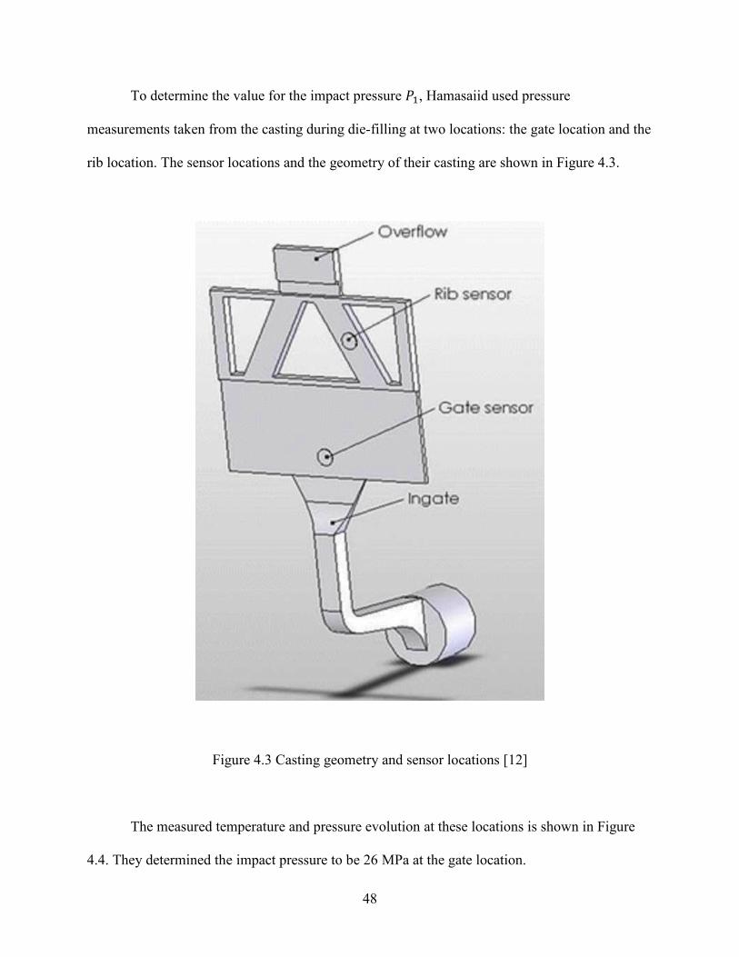
To determine the value for the impact pressure -0, Hamasaiid used pressure

measurements taken from the casting during die-filling at two locations: the gate location and the

rib location. The sensor locations and the geometry of their casting are shown in Figure 4.3.

Figure 4.3 Casting geometry and sensor locations [12]

The measured temperature and pressure evolution at these locations is shown in Figure

4.4. They determined the impact pressure to be 26 MPa at the gate location.

49

Without accounting for the capillary pressure -. and using a measured impact pressure

value of -0 = 26 MPa, the gap width estimated using this method was found to lead to estimated

peak heat fluxes 5 times too large. The comparison between the model and experimental results

for the two materials studied, A380 and AZ91D, is shown in Figure 4.5.

Figure 4.4 Temperature and pressure evolution in HPDC [12]

50

Figure 4.5 Comparison of experimental IHTC and model by Hamasaiid when neglecting the

effect capillary pressure.

4.2.4 Capillary pressure

Due to this result, Hamasaiid determined that the capillary pressure must account for the

difference between the model and the experimental results. Empirically, they determined -. to be

negative (poor wetting) and for it to follow the relation:

-. = −0.87-0 (Equation 4-9)

0

100000

200000

300000

400000

500000

600000

700000

800000

A380 AZ91D

Pe

ak I

HT

C (

W/m

2 K

)

Peak IHTC: unadjusted Hamasaiid model vs. experiment

Hamasaiid model Experiment

51

where -0 is the melt impact pressure. Using the measured impact pressure -0 = 26 MPa, -. =−22.62 MPa.

We will examine the validity of this assumption. The magnitude of the capillary pressure

can be determined from Young’s equation, if the contact angle between the die and melt is

known. This approach has been used by Prasher et al. to determine the capillary pressure

between thermal interface materials (TIM) and rough substrates. [62] They used a model

visualized in Figure 4.6 for a conical air gap in contact with a solid substrate and liquid, where +

is the angle between the cone of air and the mean plane, and , is the contact angle between melt

and the substrate.

Figure 4.6 Conical air gap model [62]

Using this air gap model, Yuan et al. [50] developed the following expression for

capillary pressure:

52

-. = ± 2)* sinl, + +m( cot +

(Equation 4-10)

where )* is the liquid surface tension.

Since the average slope of the asperity is known from the surface profile measurements

of the die surface, the only remaining unknowns are the surface tension and wetting angle.

Previous experimental studies on A380 have determined surface tension values of 1.07 N/m [49]

and 0.781 N/m [63]. The wetting angle between aluminum and uncoated steel has been

determined to be approximately 37°. [64] This would indicate good wetting conditions, counter

to the empirical assumption of Hamasaiid. However, a recent study on the wetting behavior of

aluminum alloys on H13 steel has found that the wettability is hugely affected by oxidation of

the melt, substrate temperature, effect of surface coatings on the substrate and reactions between

the melt and the substrate. [65] They found contact angles of 80° to 120° in the temperature

range of 700° C to 800° C. To determine an estimate for the magnitude of the capillary pressure,

we plotted out the absolute value of

(Equation 4-10) using parameter values in Table 4.1. The results are shown Figure 4.7.

The maximum capillary pressure (40 kPa) is 2 orders of magnitude smaller than the value

for (Equation 4-9). Therefore we argue that the empirical capillary pressure term is incorrect.

53

Table 4.1 Parameter values for capillary pressure study

Parameter Value Source

�� 1.07 [49]

�� 128.7e-6 [25]

� 0.578e-6 [25]

� 3.5e-7 [25]

Figure 4.7 Absolute value of capillary pressure using (Equation 4-10) and values from Table 4.1.

0 30 60 90 120 150 180

0

10000

20000

30000

40000

Ab

so

lute

va

lue

of ca

pill

ary

pre

ssu

re (

Pa

)

Contact angle (°)

Absolute value of capillary pressure (Pa)

54

The source of this confusion, we argue, is the misinterpretation of the impact pressure

measurements. [62] The impact pressure highlighted in Figure 4.4 appears to be measured at the

end of die filling, instead of the time of initial melt impact on the die. It may be that Hamasaiid

mistaked the early onset of the intensification pressure for the impact pressure.

4.2.5 Impact pressure

To gain a better understanding of the true magnitude of the impact pressure in the HPDC

process, we looked to literature. Chen et al. [17] suggested 2 possible models to calculate the

impact pressure of melt in HPDC. One model is the stagnation pressure, applicable for modeling

flow impingement in stagnation point flow. Stagnation point flow is fluid flow in the vicinity of

a solid surface where the flow separates into two different streams. It is given by the equation:

Δ- = 12 ��D

(Equation 4-11)

where � is the fluid density and � is the upstream flow velocity. The values given by the

stagnation pressure equation are on the order of 2e5 Pa, too small to realistically reflect the

casting metal – die impact.

Another model suggested by Chen is the water hammer pressure model. The water

hammer pressure is the pressure wave caused by the hydraulic shock of fluid changing direction

or stopping suddenly. This model successfully predicts the maximum impact pressure of droplets

on a solid surface. [66]:

55

Δ-12� = �� (Equation 4-12)

where � is the fluid sonic velocity, given by

� = �3�

(Equation 4-13)

where 3 is the bulk modulus of the fluid.

To find an estimate for the value of water hammer pressure, we looked for material

properties from literature. To determine the velocity of the flow field at the sensor locations

shown in Figure 4.3, we carried out die-filling simulations for a casting geometry based on the

experimental setup in [15] [12] [16].

4.3 Die-filling simulation

4.3.1 Goals

The goal of the die-filling simulation was to determine the flow velocity inside the die

during casting. This velocity can be used to calculate the value of the water hammer pressure,

which can then be used as an input in the IHTC model. To ensure that the mesh sizing is

sufficient for a realistic simulation, a mesh independence study was carried out. It should be

noted that the resolution of the simulation is not sufficient to describe the initial liquid metal jet

impact with the die wall with the level of detail of droplet impact simulations, but it can be used

to determine the flow velocity field in the casting. The simulations were carried out at the high-

56

performance computing cluster at the University of Alabama. The material properties used in the

simulation are found in Table 4.2. The simulation parameters for the study are found in Table

4.3. The geometry for the simulation, which takes use of symmetry, is shown in Figure 4.8.

Table 4.2 Material parameters for die-filling simulation

Material Velocity (m/s) Viscosity (Pa/s) Density (kg/m3) Bulk modulus (GPa)

Al-9Si-3Cu 0.87 0.001 [67] 2800 [25] 41.3 [68]

AZ91D 1.53 0.0015 [69] 1800 [25] 20.4 [68]

Table 4.3 Simulation parameters for die-filling simulation

Parameter

Turbulence model K-omega SST

Mesh sizing 5e-4 m, 1e-3 m

Time-step 1e-5 s

Processors 32

Double precision Yes

Calculation time 2 weeks

Solver PISO

VOF global courant number criterion 0.5-1.5

57

Figure 4.8 FLUENT simulation geometry

58

4.3.2 Mesh independence study

To make sure that the mesh size was sufficient to capture the turbulent behavior of the

metal at the die-casting boundary, a mesh independence study was carried out. Two different

mesh sizes were simulated: 1e-3 m and 5e-4 m. Both meshes are tetrahedral with no wall

inflation layers. Wall inflation layers were tried but left out, since they caused numerical

instability at the gate region. The material used was Al-9Si-3Cu and the piston velocity was 0.87

m/s.

The wall <d values and filling velocity were compared. For the k-omega SST turbulence

model, the wall <d value should optimally be ~1 to accurately model boundary phenomena. [53]

The results for the mesh independence study are shown Figure 4.9, Figure 4.10, Figure 4.11,

Figure 4.12, Figure 4.13 and Figure 4.14.

Figure 4.9 shows that the wall <d value is on the order ~10 for the fine mesh (right) and

order ~20 for the coarse mesh (left) at the gate location. We chose to use the finer mesh but not

refine it further due to calculation capacity constraints.

59

Figure 4.9 Wall <d value at t=0.075 s for coarse mesh (left), fine mesh (right), and difference

between two models (bottom).

Figure 4.10, Figure 4.11 Figure 4.12 show the simulated melt volume fraction at times 0.09 s,

0.12 s and 0.14 s after start of injection for the fine and coarse mesh. The coarse mesh has

noticeably less detail at the melt-air interface, and has a slightly different filling pattern, which is

best visible at t=0.14s.

60


(bottom) at t=0.09 s

The velocity profile in the casting for the fine and coarse mesh is shown in Figure 4.13

and Figure 4.14. The fine mesh appears to capture backflow and vortices in more detail than the

coarse mesh.

61



62



Figure 4.13 Velocity vectors for filling, time-step at 0.09 s

63

Figure 4.14 Velocity vectors for filling at time-step 0.14 s

4.3.3 Velocity at the gate and rib locations

To find an estimate for the impact pressure at the sensor areas (gate, rib) for AZ91D and

Al-9Si-3Cu, cross-sectional average velocities during filling were established at the gate and rib

location, where the pressure and temperature sensors were located. The locations are displayed in

Figure 4.15. The velocity profile for Al-9Si-3Cu at the gate location is shown in Figure 4.17. The

velocity profile for the rib location for Al-9Si-3Cu is shown in Figure 4.17. For further analysis,

the average area velocity was determined.

64

Figure 4.15 Locations for determining velocity profile

65

Figure 4.16 Gate velocity profile for Al-9Si-3Cu

Figure 4.17 Rib velocity profile for Al-9Si-3Cu

66

4.3.3 Impact pressure and IHTC

The velocity profiles were used to calculate the water hammer pressure. The IHTC was

calculated using the Hamasaiid model based on this pressure. The flow velocity was measured at

3 time steps to show that the results are not too sensitive to fluctuation during the die filling. The

resulting values for the water hammer pressure, the peak IHTC and the experimental results are

shown in Table 4.4 and Table 4.5 for the Al-alloy and Mg-alloy respectively. The impact

pressure is used to calculate the initial air gap width, which is used to calculate the peak IHTC

according to the Hamasaiid model.

The calculated impact pressures for both alloys are very similar, even though the

processing parameters and material parameters are vastly different for the two castings. This is

promising, since the experimental peak IHTC is also very similar for the two.

However, the calculated water hammer pressure is too high to give correct results. A

fitting constant related to the impact angle was used to scale the pressure. The exact impact angle

is difficult to determine from the simulation, but it can be expected to be small, since the flow is

mostly lateral to the die surface. The impact pressure of droplets has been shown to be

dominated by the surface-normal component of velocity [70]. Therefore we can make the

assumption that only the normal component of the flow velocity matters. Instead of using the full

value of the water hammer pressure, we adjust it according to the relation:

67

Δ-~>�� = Δ-12� ⋅ sin l�m (Equation 4-14)

where � is the impact angle. Using a contact angle of 3.5°, we obtain the correct estimates for

IHTC at the gate location. For comparison, the values obtained by Hamasaiid are shown in

Table 4.6 and Table 4.7. Finally, a comparison between the two models and experiments can be

seen in Figure 4.18.

The results show good agreement at the gate location. At the rib location, the deviation

from experiment may be explained by the more complicated filling pattern which makes the

impact velocity more difficult to predict. Any differences between our simulated geometry and

the actual casting geometry can cause error. Additionally, the flow at the rib location is very

turbulent and the average velocity fluctuates significantly, which may introduce errors.

Table 4.4 IHTC for Al-alloy, present study

Velocity

Water

hammer

pressure

10� Pa

Pressure

normal

component

10� Pa

Initial

Air gap

width

10w� m

Present

study IHTC

(W/m2 K)

Experimental

peak IHTC

(W/m2 K)

Gate 0.10 s 2.938 31.7 1.94 0.359 93 000 90 000

Gate 0.11 s 2.911 31.4 1.92 0.360 92 000 90 000

Gate 0.12 s 2.993 32.3 1.97 0.357 94 000 90 000

Rib 0.10 s 1.739 18.8 1.15 0.427 55 000 N/A

Rib 0.11 s 2.048 22.1 1.35 0.405 65 000 N/A

Rib 0.12 s 1.931 20.8 1.27 0.413 61 000 N/A

68

Table 4.5 IHTC for Mg-alloy, present study

Velocity

(m/s)

Water

hammer

pressure

10� Pa

Pressure

normal

component

10� Pa

Initial

Air gap

width

10w� m

Present

study

IHTC

(W/m2 K)

Experiment

al peak

IHTC

(W/m2 K)

Gate 0.05 s 5.677 34.5 2.11 0.349 92 000 100 000

Gate 0.06 s 5.453 33.1 2.02 0.354 86 000 100 000

Gate 0.07 s 5.459 33.2 2.03 0.353 86 000 100 000

Rib 0.05 s 1.656 10.0 0.614 0.817 24 000 85 000

Rib 0.06 s 3.336 20.3 1.24 0.416 54 000 85 000

Rib 0.07 s 2.867 17.4 1.06 0.439 46 000 85 000

Table 4.6 IHTC for Al-alloy, Hamasaiid

Impact pressure

10� Pa

Adjusted with

0.87*P1

10� Pa

Initial Air

gap width

10w� m

Hamasaiid model

peak IHTC

(W/m2 K)

Experimental peak

IHTC

(W/m2 K)

26 3.38 0.298 152095 90 000

Table 4.7 IHTC for Mg-alloy, Hamasaiid

Impact

pressure

10� Pa

Adjusted

with

0.87*P1

10� Pa

Initial

Air gap

width

10w� m

Hamasaiid

model peak

IHTC

(W/m2 K)

Experimental

peak IHTC

(W/m2 K)

26 3.38 0.298 136154 100 000

69

Figure 4.18 IHTC comparison between experiment, Hamasaiid model and present study.

4.4 Evolution of IHTC with time

The second goal of the paper is to create a method to implement the evolution of the

IHTC with time in HPDC in a FLUENT simulation. We assume that the air gap between the die

and casting grows as a linear function of the fraction of solid of the casting. We assume 1D

solidification. This assumption is justified for the gate area, but might not be for the rib area. The

geometry for the time evolution simulation is shown in Figure 4.19. The width of the air gap as a

function of time is given by:

( = (/ + �/� l�m (Equation 4-15)

0

20000

40000

60000

80000

100000

120000

140000

160000

Al-9Si-3Cu AZ91D

Peak IHTC at gate location

Experiment Hamasaiid Present study

70

where �/ is a fitting constant, (/ is the initial air gap width, and � is the solid fraction of the fluid

domain. The fraction of solid is calculated using an equilibrium solidification model in

FLUENT. The script files required to run the simulation are included in Appendix A-F. The

flowchart in Figure 4.20 details how to setup and run the simulation.

Figure 4.19 Geometry for IHTC evolution simulation. The casting half-thickness mesh is shown

in teal and die mesh in grey.

A �/ value of 1e-7 was found to fit both the Aluminum and Mg-alloy. The results are

shown in Figure 4.21 and Figure 4.22 with blue dots indicating experimental results, and the red

line indicating simulation results. However, both the present study and the model by Hamasaiid

ignore the effect of fluid flow on the IHTC. With a Nusselt number of 1, this may cause severe

errors. Future work should aim to validate this model while taking into account fluid flow in the

FLUENT simulation during the die-filling timeframe.

71

Figure 4.20 Flowchart for time-evolution simulation of IHTC

Apply thin-wall

boundary condition

at die-casting interface

with thermal conductivity

k=1000 W/m2

Initialize FLUENT

simulation

Insert material properties,

processing conditions

and boundary wall ID to

IHTC.scm.

Read script file

IHTC.scm to apply

initial IHTC to melt-die

boundary layer

Set FLUENT to automatically execute

"file/read evohtc.scm" at the end of

every time step

Run simulation

Results are written in

output.txt

72

Figure 4.21 time evolution of modelled IHTC (red) vs experiment (blue) for Mg-alloy

Figure 4.22 time evolution of modelled IHTC (red) vs experiment (blue) for Al-alloy

0

20000

40000

60000

80000

100000

120000

0.7 0.8 0.9 1 1.1 1.2 1.3

IHT

C (

W/m

2 K

)

time (s)

AZ91D

0

20000

40000

60000

80000

100000

120000

0.7 0.8 0.9 1 1.1 1.2 1.3 1.4

IHT

C (

W/m

2 K

)

time (s)

A380

73

4.5 Conclusions

1) The IHTC model by Hamasaiid et al. was found to contain an unrealistic empirical

capillary pressure term.

2) The impact pressure was predicted using the “water hammer pressure” model. The IHTC

values for both Mg and Al alloys matched experimental results very well, when this

pressure model was used with the addition of a scalar scaling factor. This is promising,

because the material properties and casting conditions for both alloys were very different.

3) A model for the time-evolution of the IHTC was developed and implemented in

FLUENT 18.1 using .scm script files and UDF-files. Modelling the air gap evolution as a

linear function of fraction of solid gave moderately good results. The same fitting

constant could be used for both the Mg and Al alloy

74

– SOLIDIFICATION KINETICS OF FE-RICH INTERMETALLICS

5.1 Introduction

High-pressure die-cast of Al-alloys usually add Fe (1-2%) to reduce soldering of metal to

die. However, as an unwanted side-effect, brittle iron-rich intermetallics are formed. The most

common morphology of Fe-rich intermetallics in HPDC A383 is the polyhedral �-

Al15(Fe,Mn,Cr)3Si2, shown in Figure 5.1.

These particles follow a bimodal size distribution. This is caused by two different particle

growth mechanisms. Some particles nucleate in the holding tank before the casting takes place.

The growth of these particles is not limited by diffusion, but instead by the low driving force for

growth at high temperature. These particles grow up to large sizes. [71]

Other particles nucleate interdendritically during the casting, where the segregation of Fe

and the lower temperature provides a greater driving force for phase transformation. However,

their growth is limited by impingement on the primary or eutectic phase, and possibly also by the

diffusion rate of Fe from the bulk to the liquid-intermetallic interface. The goal of the present

study is to model the latter growth mechanism.

75

Figure 5.1 Polyhedral �-Fe intermetallic (“sludge”) [36]

We introduce a method to predict the average diameter of the interdendritic �-Fe

intermetallics in A383 using the diffusion-controlled growth model by Nastac [72] combined

with solidification simulations using the commercial casting simulation software

NOVASOLID&FLOW. We validate our predictions using image analysis of optical micrographs

of various cross-sections of the casting. The strategy of the study is shown in Figure 5.2.

�-Fe intermetallics have a BCC crystal structure, and exhibit faceted growth. The

terminal faces of polyhedral �-Fe intermetallic particles belong to plane {110}, with 120° or 60°

degree angles between faces. When viewed from the 111 direction, particles appear hexagonal.

[73] These findings have led us to believe that the Fe-rich intermetallic has a rhombic

76

dodecahedron 3D-shape. [74] This observation is supported by SEM-analysis of deep-etched �-

Fe intermetallic morphology in AlSi9Cu3Fe-alloys. [71]

Figure 5.2 Strategy for �-Fe intermetallic growth study.

Simulate solidification

in HPDC A383 using

NOVAFLOW&SOLID

Model Fe-rich intermetallic

growth using classical

solidification theory

Validate model using

image analysis

of optical micrographs

77

5.2 Mathematical models

We use the Scheil equation to model the evolution of the Fe-concentration in the casting

during solidification:

4* = 4/l1 − � m�w0 (Equation 5-1)

where 4/ is the bulk liquid concentration, � is the solid fraction, and � is the partition

coefficient. This model has two major assumptions:

- Diffusion in liquid is infinitely fast.

- Diffusion in solid does not take place.

For the first assumption to be valid, the liquid diffusion must be faster than the particle

growth velocity, otherwise we will overestimate growth. The second assumption is valid, if the

solid diffusivity of Fe is significantly slower than liquid Fe diffusivity. The orders of magnitude

for liquid and solid diffusivity of Fe in Al are 1e-9 and 1e-18 respectively, which justifies this

assumption. [75]

For volume-diffusion limited growth, growth velocity of a particle is given by:

�5 = Ω ��#� − #5

(Equation 5-2)

where �� is the liquid diffusifity, #� is the radius of the micro-volume element, #5 is the radius

of the intermallic particle, and Ω is the solutal supersaturaion. The use of (Equation 5-2)

requires the assumption, that diffusion is the rate-limiting factor for intermetallic growth, instead

of the rate of chemical reaction for formation of �-Fe. To ascertain this, the Gibbs formation

78

energy of �-Fe should be known as a function of temperature. Unfortunately, to the author’s

knowledge, no such studies have been carried out to date.

Solutal supersaturation is given by the equation:

Ω = �C�* − 4*∗45∗ − 4*∗ (Equation 5-3)

where 4*∗ is the liquid interface concentration, 45∗ is the interface concentration for �-Fe, and �C�* is the average liquid concentration.

The volume of the microelement is given by:

#� = 34π p 8�95r0/q

(Equation 5-4)

where 8� is the volume of liquid in the solidification envelope, and 95 is the number of �-Fe

nuclei in that volume.

Our model assumes that the �-Fe particles are spherical. To check the validity of this

assumption, we can compare the statistical diameter distribution of spheres and rhombic

dodecahedrons using the approach and data from Danilenko et al. [76]. The results shown in

Figure 5.3 indicate that the match is adequate for all but the 10% largest and smallest diameters.

79

Figure 5.3 Comparison between statistical distribution of cross-sections of diameters for spheres

and rhombic dodecahedrons.

5.3 Predicting cooling rate in HPDC A383

Casting simulations were carried out in NOVAFLOW&SOLID to determine the time-

evolution of temperature and solid fraction in the casting. To validate the simulation, the

predicted temperature of the die surface at 6 distinct locations was compared with FLIR thermal

camera measurements taken after removal of the casting. These locations are shown in Figure 5.4

alongside the temperature profile of the die surface. These measurements were carried out at two

different stages of the casting cycle: before the application of water sprays, and after the

application of water sprays. The measured temperature values are shown in Table 5.1. The letter

A and B stand for measurements taken before the spray and after the spray respectively. The

numbers 1-6 indicate the location of the measurement.

0

0.05

0.1

0.15

0.2

0.25

0.3

0.35

0.4

0.45

0 0.2 0.4 0.6 0.8 1

Fre

qu

en

cy (

fra

ctio

n)

Relative diameter d/d_max

Statistical diameter distribution for rhombic

dodecahedrons and spheres

rhombic dodecahedron sphere

80

The NOVAFLOW&SOLID model contains subroutines for air gap evolution, water

sprays and cycling. However, in the scope of this study, it was not possible to experimentally

determine the correct parameters for these models, so we had to rely on parameter fitting.

Figure 5.4 FLIR temperature measurement of Die-surface after casting

81

Table 5.1 FLIR temperature measurements

1 2 3 4 5 6 7 8 9 10 Average

A1 334 334 314 313 339 318 322 318 322 320 323

B1 264 261 270 270 265 266 271 266 276 274 268

A2 175 175 179 179 157 187 189 187 188 186 180

B2 165 163 166 167 167 180 184 180 185 171 173

A3 334 335 348 346 339 318 322 318 322 320 330

B3 264 261 270 270 265 266 271 266 276 261 267

A4 334 334 348 346 339 318 322 318 322 320 330

B4 264 261 270 270 265 266 271 266 276 261 267

A5 112 112 112 112 124 121 123 121 105 119 116

B5 91 90 88 90 85 95 97 95 82 94 91

A6 271 271 280 279 273 285 289 285 289 286 281

B6 215 212 218 218 188 193 197 193 198 197 203

4 parameters were chosen to be varied for the fitting process:

- The die-air contact temperature

- Maximum air gap width

- Temperature of air gap formation

- Cooling channel water flow

To minimize the amount of simulations needed to establish the correct fitting parameter

values, we used orthogonal array testing (Taguchi method) [77] [78]. Orthogonal array testing

provides a systematic way to estimate the effect of multiple independent variables on the

82

outcome of a process. It is a less robust approach than ANOVA (analysis of variance), but

significantly faster. In orthogonal array testing, the user chooses a set number of independent

variables and a set number of levels for each variable. The method then provides the user with

the least number of trials required to test each pairwise combination of each variable level. For

our case, we chose 3 levels for each variable. The resulting set of trials is shown in Table 5.2.

By analyzing the simulations, we could establish the relative significance of each

parameter on the temperature evolution of locations 1-6. These results are shown in Figure 5.5

and Figure 5.6. The maximum air gap width parameter is the most significant, followed by

cooling channel water flow and the air gap formation temperature. The effect of air temperature

is insignificant.

Table 5.2 Values of optimization parameters

Trial Contact gap

(¢m)

Air gap formation

temperature (°C)

Cooling channel water

flow multiplier

Air inside die

temperature (°C)

1 100 440 1x 150

2 100 480 3x 200

3 100 520 5x 250

4 200 440 3x 250

5 200 480 5x 150

6 200 520 1x 200

7 300 440 5x 200

8 300 480 1x 250

9 300 520 3x 150

83

Figure 5.5 Relative effect of varying fitting parameters to temperatures at locations 1-6 before

water spray.

Figure 5.6 Relative effect of varying fitting parameters to temperatures at locations 1-6 after

water spray.

0

10

20

30

40

50

60

70

80

90

100

1 2 3 4 5 6

Contribution of fitting parameters temperature before spray

Air temperature inside mould (+50 C)

cooling channel water (+200%)

air gap formation temperature (+40 C)

air gap (+100 um)

0

10

20

30

40

50

60

70

80

90

100

1 2 3 4 5 6

Contribution of fitting parameters to temperature after spray

Air temperature inside mould (+50 C)

cooling channel water (+200%)

air gap formation temperature (+40 C)

air gap (+100 um)

84

To determine which trial provided us with the best results, the temperature evolution at

locations 1-6 was compared with the experimental results. It was found that trial 9 gave the best

results. The comparison between the average experimental temperature measurements and

simulated temperature evolution for trial 9 at locations 1-6 is shown in Figure 5.7, Figure 5.8,

Figure 5.9, Figure 5.10, Figure 5.11 and Figure 5.12. At some locations, the die surface

temperature drops sharply immediately after the removal of the casting. The FLIR measurements

are taken after a small delay after the opening of the die, which explains why the measurements

do not match the peak temperature in the simulation, but rather the temperatures after this rapid

drop.

85


measurements.

0 200 400 600

300

400

500

600

700T

em

pera

ture

(K

)

time (s)

Temperature (K)

Measurement A1 (K)

Measurement B1 (K)

Point 1 temperature

86


measurements.

0 200 400 600

200

300

400

500

600

700T

em

pera

ture

(K

)

time (s)

Temperature (K)

Measurement A2 (K)

Measurement B2 (K)

Point 2 temperature

87


measurements.

0 200 400 600

200

300

400

500

600

700T

em

pera

ture

(K

)

time (s)

Temperature (K)

Measurement A3 (K)

Measurement B3 (K)

Point 3 temperature

88


measurements.

0 200 400 600

200

300

400

500

600

700T

em

pera

ture

(K

)

time (s)

Temperature (K)

Measurement A4 (K)

Measurement B4 (K)

Point 4 temperature

89


measurements.

0 200 400 600

300

400

500

600

700

800T

em

pera

ture

(K

)

time (s)

Temperature (K)

Measurement A5 (K)

Measurement B5 (K)

Point 5 temperature

90


measurements.

0 200 400 600

300

400

500

600

700

800T

em

pera

ture

(K

)

time (s)

Temperature (K)

Measurement A6 (K)

Measurement B6 (K)

Point 6 temperature

91

5.4 Methods

5.4.1 Experimental methods

An as-cast A383 engine block was cut, and 5 samples were obtained for image analysis.

The samples 1,2,3 correspond to the front, center and rear of the bulkhead respectively. The

location of the samples is shown in Figure 5.13.

Figure 5.13 Location of samples for sludge size measurements

The area of each �-Fe intermetallic particle in 3 micrograph from each sample was

measured using Photoshop. Unfortunately, there were too few measurements available from

sample 2 to make a statistically relevant determination of intermetallic size, so it was ignored.

Figure 5.14 shows a micrograph taken from sample 1, the front of the bulkhead. The �-Fe

intermetallic phase is visible as light grey. The dark grey phase is eutectic silicon. The white

92

phase is primary or eutectic aluminum. Figure 5.15 shows an optical micrograph taken from

sample 5. Due to the higher cooling rate, the microstructure is finer, and silicon and sludge

particles exhibit higher circularity.

The �-Fe intermetallic diameter distribution was calculated from the measurements using

the open source Python script GrainSizeTools. We used the app to calculate and visualize the

average 2D-diameter distribution and the estimated 3D-size distribution (using the Saltykov-

method).

Figure 5.14 Optical micrograph taken from sample 1.

93

Figure 5.15 Optical micrograph taken from sample 5.

5.4.2 Growth model parameters

The solidification kinetics for the locations of samples 1, 3, 4 and 5 were determined

from the NOVAFLOW&SOLID simulation trial 9. Our hypothesis is that the growth of the �-Fe

particle starts at the liquidus temperature of the Al-aluminum, and ends at the start of eutectic

growth. The parameters used for the solidification model are shown in Table 5.3. The density of

�-Fe nuclei in the melt was unknown, so the parameters 95 and 8� were considered fitting

parameters.

94

Table 5.3 Input parameters for �-Fe growth model

Parameter Value Source

£ 0.029 [37]

¤¥ 2.7e-9 [75]

¦§ 1 wt% NEMAK Alabama

¨© 1000 Fitting parameter

ª¥ 4.2e-6 Fitting parameter

5.5 Results and discussion

5.5.1 Samples 1 and 3

Figure 5.16 shows the simulated evolution of temperature and fraction of solid for the

bulkhead edge location (samples 1 and 3). It is seen that melt reaches the solidus temperature

95

after approximately 1.2 seconds, which according to our hypothesis, is the timeframe for �-Fe

particle growth.

Figure 5.17 and Figure 5.18 show the measured diameter distributions for the �-Fe

particles. The average size is approximately 2 um. The Saltykov-method correction slightly shifts

the distribution to larger diameters, but not significantly.

Figure 5.19 shows the predicted �-Fe diameter evolution according to our solidification

model. The agreement with experiments is good.

Figure 5.16 NOVAFLOW&SOLID simulation of Samples 1,3

0 5 10 15

0

10

20

30

40

50

60

70

80

90

100

Liquid fraction (%)

Temperature (K)

Kinetic solidus temperature (K)

time (s)

Liq

uid

fra

ctio

n (

%)

300

350

400

450

500

550

600

Tem

pe

ratu

re (

K)

Sample 1,3 solidification simulation

96

Figure 5.17 Measured �-Fe diameter distribution and Saltykov-method estimate for 3D diameter

distribution for sample 1.

97



98

Figure 5.19 �-Fe growth model predicted diameter at samples 1,3

0.0 0.2 0.4 0.6 0.8 1.0 1.2

0.0

0.5

1.0

1.5

2.0

2.5

3.0S

am

ple

1,3

in

term

eta

llic d

iam

ete

r (μ

m)

Time (s)

Sample 1,3 intermetallic diameter (μm)

99

5.5.2 Sample 4

Figure 5.20 shows the simulated evolution of temperature and fraction of solid at the top

of the cylinder outer rim (sample 4). It can be seen that melt reaches the solidus temperature after

approximately 0.5 seconds.

Figure 5.21 shows the measured diameter distributions for the �-Fe particles. The

average size is approximately 1.5 um. The Saltykov-method correction slightly shifts the

distribution to larger diameters, but not significantly.


model. The agreement with experiments is good.

Figure 5.20 NOVAFLOW&SOLID simulation of Sample 4

0 1 2 3 4

0

10

20

30

40

50

60

70

80

90

100

Liquid fraction (%)

Temperature (K)


time (s)

Liq

uid

fra

ctio

n (

%)

300

350

400

450

500

550

600

Te

mp

era

ture

(K

)

Sample 4 solidification simulation

100



101

Figure 5.22 �-Fe growth model predicted diameter at sample 4

0.0 0.1 0.2 0.3 0.4 0.5 0.6

0.0

0.5

1.0

1.5

2.0

2.5

3.0S

am

ple

4 in

term

eta

llic d

iam

ete

r (μ

m)

Time (s)

Sample 4 intermetallic diameter (μm)

102

5.5.2 Sample 5

Figure 5.23 shows the simulated evolution of temperature and fraction of solid at the

inner cylinder surface (sample 4). It can be seen that melt reaches the solidus temperature after

approximately 3 seconds.

Figure 5.24 shows the measured diameter distributions for the �-Fe particles. The

average size is approximately 0.8 um. The Saltykov-method correction slightly shifts the

distribution to larger diameters, but not significantly.


model. The agreement with experiments is not good. According to the �-Fe particle size,

predicted solidification time at this location should be shorter. By looking at Figure 5.23, we can

see that the initial cooling rate is slower than in sample 4, even though the final solidification

time is similar. It may be that the NOVAFLOW&SOLID does not properly account for the effect

of the steel liners adjacent to the cylinder, or the large water cooling channel inside the cylinder.

103

In general NOVAFLOW&SOLID tends to underestimate the effect of water cooling channels, as

seen from the parameter sensitivity analysis.

Figure 5.23 NOVAFLOW&SOLID simulation of Sample 5

0 1 2 3 4 5 6

0

10

20

30

40

50

60

70

80

90

100

Liquid fraction (%)

Temperature (K)


time (s)

Liq

uid

fra

ctio

n (

%)

300

350

400

450

500

550

600

Te

mp

era

ture

(K

)

Sample 5 solidification simulation

104



105

Figure 5.25 �-Fe growth model predicted diameter at sample 5

0.0 0.5 1.0 1.5 2.0 2.5 3.0

0.0

0.5

1.0

1.5

2.0

2.5

3.0S

am

ple

5 in

term

eta

llic d

iam

ete

r (μ

m)

Time (s)

Sample 5 intermetallic diameter (μm)

106

5.6 Conclusions

1) Orthogonal array testing was used to determine fitting parameter values for simulating

A383 HPDC heat transfer.

2) The Saltykov-method 3D-adjusted �-Fe diameter distribution does not significantly differ

from the 2D distribution.

3) The average particle diameter is 2.1, 1.6, 1.5, 0.8 um for samples 1,3,4,5 respectively.

4) The �-Fe growth model was able to predict the average size for �-Fe diameter for

samples 1,3 and 4. For sample 5, it seems as if the NOVASOLID&FLOW underestimates

heat transfer near the cylinder, and thus over-predicts intermetallic size.

5) The number of samples is not sufficient to definitively determine the growth mechanism

of the �-Fe particle. However, this study forms a good framework for further experiments

and simulations.

107

– CONCLUSIONS AND FUTURE WORK

6.1 Conclusions

6.1.1 Water cooling channels

1) A model based on the Gnielinski correlation was developed. It is capable of predicting

the Nu-number of bubbler water-cooling channels within 15% margin of error for

6000<Re<25000 and channel diameters up to 5 mm.

2) This model can be used to validate water channel models in simulation softwares such as

FLUENT or NOVAFLOW&SOLID. This is especially important in the case of

commercial software, since their underlying implementation of heat transfer coefficients

is usually unknown. This correlation can be used to validate the results of these black box

models.

6.1.2 Die-casting interfacial heat transfer coefficient

1) The IHTC model by Hamasaiid et al. was found to contain an unrealistic empirical

capillary pressure term.

2) The impact pressure was predicted using the “water hammer pressure” model. The IHTC

values for both Mg and Al alloys matched experimental results very well, when this

108

3) pressure model was used. This is promising, because the material properties and casting

conditions for both alloys were very different.

4) A model for the time-evolution of the IHTC was developed and implemented in

FLUENT 18.1 using .scm script files and UDF-files. Modelling the air gap evolution as a

linear function of fraction of solid gave moderately good results. The same fitting

constant could be used for both the Mg and Al alloy.

6.1.3 Kinetics of �-Fe intermetallic growth in HPDC A383

1) Orthogonal array testing was successfully used to determine fitting parameter values and

parameter sensitivity for simulating A383 HPDC heat transfer using

NOVAFLOW&SOLID.

2) Measured sludge diameter distribution were compared with sizes calculated using

numerical solvers for cooling rates and classical solidification theory for particle growth.

3) The average particle diameter is 2.1, 1.6, 1.5, 0.8 um for samples 1,3,4,5 respectively.

4) The �-Fe growth model was able to predict the average size for �-Fe diameter for

samples 1,3 and 4. For sample 5, it seems as if the NOVASOLID&FLOW underestimates

heat transfer near the cylinder, and thus over-predicts intermetallic size.

5) The difference between the measured 2D diameters and the corrected estimated 3D

diameters using the Saltykov-method was found to be minor.

109

6.2 Main contributions of this study

1) Developed an empirical model for Nusselt number in water cooling channels. This can be

used to validate heat transfer coefficients for water cooling channels in commercial

software to assist in modelling heat transfer in the HPDC process.

2) Developed a model for impact pressure in HPDC, which augments the Hamasaiid model

for peak IHTC in HPDC and gives better results than their previous model.

3) Developed a method to integrate the Hamasaiid IHTC model as a boundary condition in

FLUENT 18.1 using .scm and UDF-files.

4) Predicted size of polyhedral Fe-rich intermetallics using commercial casting simulation

NOVAFLOW&SOLID for cooling rates and classical solidification theory for

intermetallic size. This study lays the framework for how to combine commercial casting

simulation software and micrograph measurements to make quantitative predictions of

microstructure.

6.3 Recommendations for future work

To further validate the Hamasaiid IHTC model and the impact pressure model of the

present study, experiments should be performed with metal jet/droplet striking substrates of

varying roughness with varying velocity.

To estimate the impact of fluid flow on the IHTC model, simulations should be carried

out with varying flow velocity profiles and surface roughness values to estimate the magnitude

of the error caused by ignoring convection in our model.

110

To validate the heat transfer coefficients used in commercial casting software,

comparisons between the models established in the present study and various commercial casting

simulation software should be carried out. The findings should be validated with experimental

measurements of heat transfer in high-pressure die-castings.

Once the models are validated, the microstructure evolution in the A383 casting should

be revisited, and more sophisticated phase transformation models such as the phase field method

should be used and compared with classical solidification models.

111

REFERENCES

[1] G. Timelli and A. Fabrizi, "The Effects of Microstructure Heterogeneities and Casting

Defects on the Mechanical Properties of High-Pressure Die-Cast AlSi9Cu3(Fe) Alloys,"

Metallurgical and Materials Transactions A, vol. 45, pp. 5486-5498, November 01 2014.

[2] S. Otarawanna, H. I. Laukli, C. M. Gourlay, and A. K. Dahle, "Feeding Mechanisms in

High-Pressure Die Castings," Metallurgical and Materials Transactions A, vol. 41, pp.

1836-1846, July 01 2010.

[3] A. Long, D. Thornhill, C. Armstrong, and D. Watson, "Determination of the heat transfer

coefficient at the metal-die interface for high pressure die cast AlSi9Cu3Fe," Applied

Thermal Engineering, vol. 31, pp. 3996-4006, Dec 2011.

[4] F. Bonollo, N. Gramegna, and G. Timelli, "High-Pressure Die-Casting: Contradictions

and Challenges," JOM, vol. 67, pp. 901-908, May 01 2015.

[5] W. D. Callister and D. G. Rethwisch, Fundamentals of Materials Science and

Engineering: An Integrated Approach, 5th Edition: Wiley, 2016.

[6] Y. Hangai and S. Kitahara, "Quantitative evaluation of porosity in aluminum alloy die

castings by fractal analysis of spatial distribution of area," Materials & Design, vol. 30,

pp. 1169-1173, Apr 2009.

[7] G. Lasko, M. Apel, A. Carre, U. Weber, and S. Schmauder, "Effect of Microstructure and

Hydrogen Pores on the Mechanical Behavior of an Al7%Si0.3%Mg Alloy Studied by a

Combined Phase-Field and Micromechanical Approach," Advanced Engineering

Materials, vol. 14, pp. 236-247, Apr 2012.

[8] A. Carre, B. Bottger, and M. Apel, "Phase-field modelling of gas porosity formation

during the solidification of aluminium," International Journal of Materials Research, vol.

101, pp. 510-514, Apr 2010.

[9] F. P. Incropera, Fundamentals of Heat and Mass Transfer: John Wiley \&\#38; Sons,

Inc., 2006.

[10] H. Herwig, "What Exactly is the Nusselt Number in Convective Heat Transfer Problems

and are There Alternatives?," Entropy, vol. 18, May 2016.

112

[11] D. D. Ndenguma, J. Dirker, and J. P. Meyer, "Heat transfer and pressure drop in annuli

with approximately uniform internal wall temperatures in the transitional flow regime,"

International Journal of Heat and Mass Transfer, vol. 111, pp. 429-441, 2017.

[12] A. Hamasaiid, G. Dour, M. S. Dargusch, T. Loulou, C. Davidson, and G. Savage, "Heat-

transfer coefficient and in-cavity pressure at the casting-die interface during high-

pressure die casting of the magnesium alloy AZ91D," Metallurgical and Materials

Transactions a-Physical Metallurgy and Materials Science, vol. 39a, pp. 853-864, Apr

2008.

[13] G. Dour, M. Dargusch, C. Davidson, and A. Nef, "Development of a non-intrusive heat

transfer coefficient gauge and its application to high pressure die casting - Effect of the

process parameters," Journal of Materials Processing Technology, vol. 169, pp. 223-233,

Nov 10 2005.

[14] Z. P. Guo, S. M. Xiong, B. C. Liu, M. Li, and J. Allison, "Effect of Process Parameters,

Casting Thickness, and Alloys on the Interfacial Heat-Transfer Coefficient in the High-

Pressure Die-Casting Process," Metallurgical and Materials Transactions a-Physical

Metallurgy and Materials Science, vol. 39a, pp. 2896-2905, Dec 2008.

[15] M. S. Dargusch, A. Hamasaiid, G. Dour, T. Loulou, C. J. Davidson, and D. H. St John,

"The accurate determination of heat transfer coefficient and its evolution with time

during high pressure die casting of Al-9%Si-3%Cu and Mg-9%Al-1%Zn alloys,"

Advanced Engineering Materials, vol. 9, pp. 995-999, Nov 2007.

[16] A. Hamasaiid, G. Wang, C. Davidson, G. Dour, and M. S. Dargusch, "Interfacial Heat

Transfer during Die Casting of an Al-Si-Cu Alloy," Metallurgical and Materials

Transactions A, vol. 40, p. 3056, 2009/10/27 2009.

[17] Z. W. Chen, "Skin solidification during high pressure die casting of Al–11Si–2Cu–1Fe

alloy," Materials Science and Engineering: A, vol. 348, pp. 145-153, 2003/05/15/ 2003.

[18] A. Hamasaiid, M. S. Dargusch, T. Loulou, and G. Dour, "A predictive model for the

thermal contact resistance at liquid–solid interfaces: Analytical developments and

validation," International Journal of Thermal Sciences, vol. 50, pp. 1445-1459,

2011/08/01/ 2011.

[19] Y. Cao, Z. Guo, and S. Xiong, "Determination of the metal/die interfacial heat transfer

coefficient of high pressure die cast B390 alloy," IOP Conference Series: Materials

Science and Engineering, vol. 33, p. 012010, 2012/07/03 2012.

[20] W. D. Griffiths and K. Kawai, "The effect of increased pressure on interfacial heat

transfer in the aluminium gravity die casting process," Journal of Materials Science, vol.

45, pp. 2330-2339, 2010/05/01 2010.

113

[21] S. Mirbagheri, M. Shrinparvar, and A. Chirazi, "Modeling of metalo-static pressure on

the metal–mould interface thermal resistance in the casting process," Materials & design,

vol. 28, pp. 2106-2112, 2007.

[22] W.-w. Zhang, Y.-l. Zhao, D.-t. Zhang, Z.-q. Luo, C. Yang, and Y.-y. Li, "Effect of Si

addition and applied pressure on microstructure and tensile properties of as-cast Al-5.0

Cu-0.6 Mn-1.2 Fe alloys," Trans. Nonferrous Met. Soc. China, vol. 28, p. 1072, 2018.

[23] M. C. Flemings, "Behavior of metal alloys in the semisolid state," Metallurgical

Transactions A, vol. 22, pp. 957-981, 1991/05/01 1991.

[24] W.-b. Yu, S. Liang, Y.-y. Cao, X.-b. Li, Z.-p. Guo, and S.-m. Xiong, "Interfacial heat

transfer behavior at metal/die in finger-plated casting during high pressure die casting

process," China Foundry, vol. 14, pp. 258-264, July 01 2017.

[25] A. Hamasaiid, G. Dour, T. Loulou, and M. S. Dargusch, "A predictive model for the

evolution of the thermal conductance at the casting–die interfaces in high pressure die

casting," International Journal of Thermal Sciences, vol. 49, pp. 365-372, 2010/02/01/

2010.

[26] M. Qi, Y. Kang, Q. Qiu, W. Tang, J. Li, and B. Li, "Microstructures, mechanical

properties, and corrosion behavior of novel high-thermal-conductivity hypoeutectic Al-Si

alloys prepared by rheological high pressure die-casting and high pressure die-casting,"

Journal of Alloys and Compounds, vol. 749, pp. 487-502, 2018/06/15/ 2018.

[27] M.-f. Qi, Y.-l. Kang, and G.-m. Zhu, "Microstructure and properties of rheo-HPDC Al-

8Si alloy prepared by air-cooled stirring rod process," Transactions of Nonferrous Metals

Society of China, vol. 27, pp. 1939-1946, 2017/09/01/ 2017.

[28] E. Brosh, G. Makov, and R. Z. Shneck, "Application of CALPHAD to high pressures,"

Calphad-Computer Coupling of Phase Diagrams and Thermochemistry, vol. 31, pp. 173-

185, Jun 2007.

[29] J. J. Sobczak, L. Drenchev, and R. Asthana, "Effect of pressure on solidification of

metallic materials," International Journal of Cast Metals Research, vol. 25, pp. 1-14,

2012/01/01 2012.

[30] S. G. Shabestari and J. E. Gruzleski, "The Effect of Solidification Condition and

Chemistry on the Formation and Morphology of Complex Intermetallic Compounds in

Aluminium—Silicon Alloys," Cast Metals, vol. 6, pp. 217-224, 1994/01/01 1994.

[31] S. Ji, W. Yang, F. Gao, D. Watson, and Z. Fan, "Effect of iron on the microstructure and

mechanical property of Al–Mg–Si–Mn and Al–Mg–Si diecast alloys," Materials Science

and Engineering: A, vol. 564, pp. 130-139, 2013/03/01/ 2013.

114

[32] H. Z. Ye, "An overview of the development of Al-Si-alloy based material for engine

applications," Journal of Materials Engineering and Performance, vol. 12, pp. 288-297,

Jun 2003.

[33] M. Javidani and D. Larouche, "Application of cast Al–Si alloys in internal combustion

engine components," International Materials Reviews, vol. 59, pp. 132-158, 2014/04/01

2014.

[34] J. Eiken, M. Apel, S. M. Liang, and R. Schmid-Fetzer, "Impact of P and Sr on

solidification sequence and morphology of hypoeutectic Al-Si alloys: Combined

thermodynamic computation and phase-field simulation," Acta Materialia, vol. 98, pp.

152-163, Oct 1 2015.

[35] S. W. Choi, Y. M. Kim, K. M. Lee, H. S. Cho, S. K. Hong, Y. C. Kim, et al., "The effects

of cooling rate and heat treatment on mechanical and thermal characteristics of Al-Si-Cu-

Mg foundry alloys," Journal of Alloys and Compounds, vol. 617, pp. 654-659, Dec 25

2014.

[36] T. Liu, S. Morales, M. Karkkainen, L. Nastac, V. Arvikar, I. Levin, et al., "The combined

effects of Sr additions and heat treatment on the microstructure and mechanical properties

of high pressure die cast A383 alloy," Materials Science and Engineering: A, 2019.

[37] J. A. Taylor, "Iron-Containing Intermetallic Phases in Al-Si Based Casting Alloys,"

Procedia Materials Science, vol. 1, pp. 19-33, 2012/01/01/ 2012.

[38] S. Ferraro and G. Timelli, "Influence of Sludge Particles on the Tensile Properties of Die-

Cast Secondary Aluminum Alloys," Metallurgical and Materials Transactions B, vol. 46,

pp. 1022-1034, 2015/04/01 2015.

[39] M. Timpel, N. Wanderka, R. Grothausmann, and J. Banhart, "Distribution of Fe-rich

phases in eutectic grains of Sr-modified Al–10wt.% Si–0.1wt.% Fe casting alloy,"

Journal of Alloys and Compounds, vol. 558, pp. 18-25, 2013/05/05/ 2013.

[40] G. Timelli, A. Fabrizi, S. Capuzzi, F. Bonollo, and S. Ferraro, "The role of Cr additions

and Fe-rich compounds on microstructural features and impact toughness of

AlSi9Cu3(Fe) diecasting alloys," Materials Science and Engineering: A, vol. 603, pp. 58-

68, 2014/05/06/ 2014.

[41] S. Roy, L. Allard, A. Rodriguez, T. Watkins, and A. Shyam, "Comparative Evaluation of

Cast Aluminum Alloys for Automotive Cylinder Heads: Part I-Microstructure

Evolution," Metallurgical and Materials Transactions a-Physical Metallurgy and

Materials Science, vol. 48a, pp. 2529-2542, May 2017.

[42] F. Jiahong, "Uncertainty quantification on industrial high pressure die casting process,"

Open Access Theses, vol. 849, 2016.

115

[43] J. A. Dantzig and M. Rappaz, Solidification, 1st ed ed.: EPFL Press ; London : Taylor &

Francis [distributor], 2009.

[44] E. Anglada, A. Meléndez, I. Vicario, E. Arratibel, and I. Aguillo, "Adjustment of a High

Pressure Die Casting Simulation Model Against Experimental Data," Procedia

Engineering, vol. 132, pp. 966-973, 2015/01/01/ 2015.

[45] L. Zhang, L. Li, H. Ju, and B. Zhu, "Inverse identification of interfacial heat transfer

coefficient between the casting and metal mold using neural network," Energy

Conversion and Management, vol. 51, pp. 1898-1904, 2010/10/01/ 2010.

[46] R. Helenius, O. Lohne, L. Arnberg, and H. I. Laukli, "The heat transfer during filling of a

high-pressure die-casting shot sleeve," Materials Science and Engineering a-Structural

Materials Properties Microstructure and Processing, vol. 413, pp. 52-55, Dec 15 2005.

[47] Z. P. Guo, S. M. Xiong, B. C. Liu, L. Mei, and J. Allison, "Determination of the heat

transfer coefficient at metal-die interface of high pressure die casting process of AM50

alloy," International Journal of Heat and Mass Transfer, vol. 51, pp. 6032-6038, Dec

2008.

[48] Y. Cao, Z. Guo, and S. Xiong, "Determination of interfacial heat transfer coefficient and

its application in high pressure die casting process," China Foundry, vol. 11, pp. 314-321,

// 2014.

[49] M. Xue, Y. Heichal, S. Chandra, and J. Mostaghimi, "Modeling the impact of a molten

metal droplet on a solid surface using variable interfacial thermal contact resistance,"

Journal of Materials Science, vol. 42, pp. 9-18, 2007/01/01 2007.

[50] C. Yuan, B. Duan, L. Li, B. Shang, and X. Luo, "An improved model for predicting

thermal contact resistance at liquid–solid interface," International Journal of Heat and

Mass Transfer, vol. 80, pp. 398-406, 2015/01/01/ 2015.

[51] S. C. Somé, D. Delaunay, and V. Gaudefroy, "Comparison and validation of thermal

contact resistance models at solid–liquid interface taking into account the wettability

parameters," Applied Thermal Engineering, vol. 61, pp. 531-540, 2013/11/03/ 2013.

[52] L. Davidson, "An introduction to turbulence models," 2015.

[53] C. Argyropoulos and N. Markatos, "Recent advances on the numerical modelling of

turbulent flows," Applied Mathematical Modelling, vol. 39, pp. 693-732, 2015.

[54] A. Fluent, "17.1: User’s guide. ANSYS," ed: Inc.

[55] V. Gnielinski, "On heat transfer in tubes," International Journal of Heat and Mass

Transfer, vol. 63, pp. 134-140, 2013.

116

[56] B. Petukhov, "Heat transfer and friction in turbulent pipe flow with variable physical

properties," in Advances in heat transfer. vol. 6, ed: Elsevier, 1970, pp. 503-564.

[57] V. Gnielinski, "Turbulent Heat Transfer in Annular Spaces-A New Comprehensive

Correlation," Heat Transfer Engineering, vol. 36, pp. 787-789, Jun 13 2015.

[58] W. R. Van Zyl, J. Dirker, and J. P. Meyer, "Single-phase convective heat transfer and

pressure drop coefficients in concentric annuli," Heat Transfer Engineering, vol. 34, pp.

1112-1123, 2013.

[59] D. R. Poirier and G. Geiger, Transport phenomena in materials processing: Springer,

2016.

[60] Y. Heichal and S. Chandra, "Predicting thermal contact resistance between molten metal

droplets and a solid surface," Journal of Heat Transfer-Transactions of the Asme, vol.

127, pp. 1269-1275, Nov 2005.

[61] M. G. Cooper, B. B. Mikic, and M. M. Yovanovich, "Thermal contact conductance,"

International Journal of Heat and Mass Transfer, vol. 12, pp. 279-300, 1969/03/01/

1969.

[62] R. S. Prasher, "Surface chemistry and characteristics based model for the thermal contact

resistance of fluidic interstitial thermal interface materials," Journal of Heat Transfer-

Transactions of the Asme, vol. 123, pp. 969-975, Oct 2001.

[63] S.-H. Park, Y.-S. Um, C.-H. Kum, and B.-Y. Hur, "Thermophysical properties of Al and

Mg alloys for metal foam fabrication," Colloids and Surfaces A: Physicochemical and

Engineering Aspects, vol. 263, pp. 280-283, 2005/08/01/ 2005.

[64] M. Gatzen, T. Radel, C. Thomy, and F. Vollertsen, "The Role of Zinc Layer During

Wetting of Aluminium on Zinc-coated Steel in Laser Brazing and Welding," Physics

Procedia, vol. 56, pp. 730-739, 2014/01/01/ 2014.

[65] B. Wang, "Investigation of the adhesion behavior of aluminum on various PVD coatings

applied to H13 tool steel to minimize or eliminate lubrication during high pressure die

casting, An," Colorado School of Mines. Arthur Lakes Library, 2016.

[66] Y. Tatekura, M. Watanabe, K. Kobayashi, and T. Sanada, "Pressure generated at the

instant of impact between a liquid droplet and solid surface," Royal Society open science,

vol. 5, p. 181101, 2018.

[67] D. Wang and R. A. Overfelt, "Oscillating Cup Viscosity Measurements of Aluminum

Alloys: A201, A319 and A356," International Journal of Thermophysics, vol. 23, pp.

1063-1076, 2002/07/01 2002.

117

[68] P. Thakor, V. Patel, B. Thakore, P. Gajjar, and A. Jani, "Bulk modulus of some simple

liquid metals," 2008.

[69] S. J. Roach and H. Henein, "Physical Properties of AZ91D Measured Using the Draining

Crucible Method: Effect of SF6," International Journal of Thermophysics, vol. 33, pp.

484-494, 2012/03/01 2012.

[70] J. Xiong, S. Koshizuka, and M. Sakai, "Numerical Analysis of Droplet Impingement

Using the Moving Particle Semi-implicit Method," Journal of Nuclear Science and

Technology, vol. 47, pp. 314-321, 2010/03/01 2010.

[71] S. Ferraro, A. Fabrizi, and G. Timelli, "Evolution of sludge particles in secondary die-

cast aluminum alloys as function of Fe, Mn and Cr contents," Materials Chemistry and

Physics, vol. 153, pp. 168-179, 2015/03/01/ 2015.

[72] L. Nastac and D. M. Stefanescu, "Computational modeling of NbC/laves formation in

INCONEL 718 equiaxed castings," Metallurgical and Materials Transactions A, vol. 28,

pp. 1582-1587, 1997/07/01 1997.

[73] Z. Que, Y. Wang, and Z. Fan, "Formation of the Fe-Containing Intermetallic Compounds

during Solidification of Al-5Mg-2Si-0.7Mn-1.1Fe Alloy," Metallurgical and Materials

Transactions A, vol. 49, pp. 2173-2181, 2018/06/01 2018.

[74] A. Redjaïmia, A. Proult, P. Donnadieu, and J. Morniroli, "Morphology, crystallography

and defects of the intermetallic χ-phase precipitated in a duplex (δ+ γ) stainless steel,"

Journal of materials science, vol. 39, pp. 2371-2386, 2004.

[75] N. Lee and J. Cahoon, "Interdiffusion of Copper and Iron in Liquid Aluminum," Journal

of Phase Equilibria and Diffusion, vol. 32, pp. 226-234, 2011/06/01 2011.

[76] T. Danilenko, "Method for the simulation and reconstruction of 3D particle size

distributions in metal structures," in MATEC Web of Conferences, 2018, p. 01002.

[77] V. R. Joseph, "Taguchi's approach to robust parameter design: A new perspective," IIE

Transactions, vol. 39, pp. 805-810, 2007/05/28 2007.

[78] P. K. H. Lin, L. P. Sullivan, and G. Taguchi, "Using Taguchi Methods in Quality

Engineering," Quality Progress, vol. 23, pp. 55-59, Sep 1990.

118

APPENDIX A

;;; SCHEME FILE FOR CALCULATING INITIAL HTC for A380

;;; AUTHOR: Mikko Karkkainen

;;; Initialize variable for initial thickness and total thickness

(rp-var-define 'thickness 0 'real #f)

(rp-var-define 'total_thickness 0.002 'real #f)

;;; Initialize variable for air gap

(rp-var-define 'y_0 0 'real #f)

;;; Initialize fitting constant for evolution

(rp-var-define 'c 0.0000001 'real #f)

(rp-var-define 'k_res 1000 'real #f)

;;; Initialize material and processing parameters

(rp-var-define 'pi 3.14159265358979323846 'real #f)

(rp-var-define 'v 2.9 'real #f) ;; cast metal impact velocity

(rp-var-define 'wave_speed 3840.0 'real #f) ;; sonic wave speed in melt

(rp-var-define 'rho 2830.0 'real #f) ;; cast metal densit

119

(rp-var-define 'impact_angle 0.061 'real #f); // Impact angle in radians

(rp-var-define 'k_m 29.0 'real #f) ;; mould thermal conductivity

(rp-var-define 'k_c 109.0 'real #f) ;; cast metal thermal conductivity

(rp-var-define 'r_sm (* 128.7 (expt 10.0 -6.0)) 'real #f) ;; Mean peak spacing

(rp-var-define 'sigma (* 0.578 (expt 10.0 -6.0)) 'real #f) ;; Mean peak height deviation

(rp-var-define 'epsilon 1.5 'real #f) ;; numerical parameter

(rp-var-define 'p_0 101325 'real #f) ;; NTP pressure

(rp-var-define 't_1 860.0 'real #f) ;; impact temperature

(rp-var-define 't_0 300.0 'real #f) ;; NTP temperature

;;; ;;; Initialize variable for the wall zone id and shadow wall id of the thin-wall

(rp-var-define 'wall_id 4 'real #f)

(rp-var-define 'shadow_wall_id 15 'real #f)

;;; Run DEFINE_ON_DEMAND(initial_htc) to calculate the value of wall thickness and assign

it in the variable 'thickness

(%udf-on-demand 'ihtc::libudf)

;;; Run the menu command to apply the initial wall thickness to the thin-wall

(ti-menu-load-string (string-append "def bc wall" " " (number->string (%rpgetvar 'wall_id)) " "

(number->string (%rpgetvar 'thickness)) ",,,,,,,")

120

APPENDIX B

;;; SCHEME FILE FOR CALCULATING INITIAL HTC for AZ91D


;;; Initialize variable for virtual wall thickness

(rp-var-define 'thickness 0 'real #f)

;;; Initialize variable for air gap

(rp-var-define 'y_0 0 'real #f)

;;; Initialize fitting constant for evolution

(rp-var-define 'c 0.0000001 'real #f)

(rp-var-define 'k_res 1000 'real #f)

;;; Initialize material and processing parameters

(rp-var-define 'pi 3.14159265358979323846 'real #f)

(rp-var-define 'v 5.7 'real #f) ;; cast metal impact velocity

(rp-var-define 'wave_speed 3357.0 'real #f) ;; sonic wave speed in melt

(rp-var-define 'rho 1810.0 'real #f) ;; cast metal density

121

(rp-var-define 'impact_angle 0.061 'real #f); // Impact angle in radians

(rp-var-define 'k_m 29.0 'real #f) ;; mould thermal conductivity

(rp-var-define 'k_c 70.0 'real #f) ;; melt thermal conductivity

(rp-var-define 'r_sm (* 128.7 (expt 10.0 -6.0)) 'real #f) ;; Mean peak spacing

(rp-var-define 'sigma (* 0.578 (expt 10.0 -6.0)) 'real #f) ;; Mean peak height deviation

(rp-var-define 'epsilon 1.5 'real #f) ;; numerical parameter

(rp-var-define 'p_0 101325 'real #f) ;; NTP pressure

(rp-var-define 't_1 880.0 'real #f) ;; impact temperature

(rp-var-define 't_0 300.0 'real #f) ;; NTP temperature

;;; ;;; Initialize variable for the wall zone id and shadow wall id of the thin-wall

(rp-var-define 'wall_id 4 'real #f)

(rp-var-define 'shadow_wall_id 15 'real #f)

;;; Run DEFINE_ON_DEMAND(initial_htc) to calculate the value of wall thickness and assign


(%udf-on-demand 'ihtc::libudf)

;;; Run the menu command to apply the initial wall thickness to the thin-wall


(number->string (%rpgetvar 'thickness)) ",,,,,,,

122

APPENDIX C

DEFINE_ON_DEMAND(ihtc)

{

real PI = RP_Get_Real("pi");

real v = RP_Get_Real("v"); // cast metal impact velocity

real wave_speed = RP_Get_Real("wave_speed"); // sonic wave speed melt

real rho = RP_Get_Real("rho"); // cast metal density

real impact_angle = RP_Get_Real("impact_angle"); // Impact angle in degrees

real k_m = RP_Get_Real("k_m"); // mould thermal conductivity

real k_c = RP_Get_Real("k_c"); // cast metal thermal conductivity

real r_sm = RP_Get_Real("r_sm"); // Mean peak spacing

real sigma = RP_Get_Real("sigma"); // Mean peak height deviation

real epsilon = RP_Get_Real("epsilon"); // numerical parameter

real p_0 = RP_Get_Real("p_0"); // NTP pressure

real T_1 = RP_Get_Real("t_1"); // impact temperature

real T_0 = RP_Get_Real("t_0"); // NTP temperature

real y; // air gap thickness

real p_1; // water hammer pressure

123

real alpha; // helper variable

real lambda; // Effective thermal conductivity

real n; // mean of density of microcontact points

real a; // mean of contact point area

real h; // htc

real dx; // thickness of wall layer

FILE* fp;

Domain *d = Get_Domain(1); // Calculation domain

Thread *t1,*t0;

int zone_id = RP_Get_Real("wall_id"); // wall zone id (defined in

initial_htc.scm)

int shadow_zone_id = RP_Get_Real("shadow_wall_id");; // shadow wall zone id (defined in

initial_htc.scm)

t1 = Lookup_Thread(d,zone_id); // Determine face thread for wall

t0 = Lookup_Thread(d,shadow_zone_id); // Determine face thread for shadow wall

// Calculate wall thickness based on corrected Hamasaiid model

lambda = 2*k_m*k_c/(k_m+k_c);

p_1 = v*wave_speed*rho*sin(impact_angle);

y = pow(2.0,1.0/2.0)/pow(double(PI),1.0/6.0)*pow(double(p_0*T_1/(p_1*T_0)),1.0/3.0)*sigma;

alpha = y/(pow(2,1.0/2.0)*sigma);

n = 8*(1-erf(alpha))/(pow(PI,2)*epsilon*pow(r_sm,2));

124

a = 1.0/4.0*r_sm*(2*exp(-pow(double(alpha),2.0))+(pow(double(2*PI),1.0/2.0)*y*(-

1+erf(alpha))/sigma));

h = 2*lambda*a*n/pow(double(1-2*a/r_sm),3.0/2.0);

dx = RP_Get_Real("k_res")/h;

RP_Set_Real("y_0", y);

RP_Set_Real("thickness", dx);

// Print results in file output.txt

fp = fopen("output.txt","a");

fprintf(fp,"flow-time fs q h\n")

fprintf(fp,"%g %g %g %g\n", RP_Get_Real("flow-time"), 0, 0, h);

fclose(fp);

}

125

APPENDIX D

;;; SCHEME FILE FOR CALCULATING AND APPLYING HTC EVERY TIME STEP


;;; Run DEFINE_ON_DEMAND(evolve_htc) to calculate the value of wall thickness and assign


(%udf-on-demand 'evolve_htc::libudf)

;;; Calculate volume average of solid fraction of fluid zone

(%fill-node-values 'liquid-fraction)

(rp-var-define 'fl (%volume-integrals 'volume-average '(5) "liquid fraction") 'real #f)

;;; Run the menu command to apply the initial wall thickness to the thin-wall (needs to be

performed every time step)


(number->string (%rpgetvar 'thickness)) ",,,,,,,"))

126

APPENDIX E

DEFINE_ON_DEMAND(evolve_htc)

{

real PI = RP_Get_Real("pi");

real v = RP_Get_Real("v"); // cast metal impact velocity

real wave_speed = RP_Get_Real("wave_speed"); // sonic wave speed in H13 steel mould

real rho = RP_Get_Real("rho"); // cast metal density

real impact_angle = RP_Get_Real("impact_angle"); // Impact angle in degrees

real k_m = RP_Get_Real("k_m"); // mould thermal conductivity

real k_c = RP_Get_Real("k_c"); // cast metal thermal conductivity

real r_sm = RP_Get_Real("r_sm"); // Mean peak spacing

real sigma = RP_Get_Real("sigma"); // Mean peak height deviation

real epsilon = RP_Get_Real("epsilon"); // numerical parameter

real p_0 = RP_Get_Real("p_0"); // NTP pressure

real T_1 = RP_Get_Real("t_1"); // Melt impact temperature

real T_0 = RP_Get_Real("t_0"); // NTP temperature

real dx; // wall thickness value corresponding thermal resistance

127

real temp1; // mean wall temperature via mean_temp function

real temp2; // mean shadow wall temperature via mean_temp function

real f_s = 0; // fraction of solid

FILE *fp; // output file variable

real p_1; // water hammer pressure

real alpha; // helper variable

real lambda; // Effective thermal conductivity

real n; // mean of density of microcontact points

real a; // mean of contact point area

real h; // htc

Domain *d = Get_Domain(1); // Calculation domain

int zone_id = RP_Get_Real("wall_id"); // wall zone id

int shadow_zone_id = RP_Get_Real("shadow_wall_id"); // shadow wall zone id

face_t f; // wall face

Thread *t1,*t2; // Wall thread, interior wall cell thread

t1 = Lookup_Thread(d,zone_id); // Determine face thread for wall

t2 = Lookup_Thread(d,shadow_zone_id); // Determine face thread for shadow wall

real q; // heat flux over area

real y = RP_Get_Real("y_0"); // air gap width

real c = RP_Get_Real("c"); // air gap evolution constant

128

dx = RP_Get_Real("thickness");

temp2 = mean_wall_temp(t1);

temp1 = mean_wall_temp(t2);

q= (temp1-temp2)/ dx;

f_s = 1-RP_Get_Real("fl"); //get updated fraction of solid

y += c*f_s; // update air gap width

// Calculate new wall thickness based on updated air gap width using corrected Hamasaiid model

lambda = 2*k_m*k_c/(k_m+k_c);

alpha = y/(pow(2,1.0/2.0)*sigma);

n = 8*(1-erf(alpha))/(pow(PI,2)*epsilon*pow(r_sm,2));

a = 1.0/4.0*r_sm*(2*exp(-pow(double(alpha),2.0))+(pow(double(2*PI),1.0/2.0)*y*(-

1+erf(alpha))/sigma));

h = 2*lambda*a*n/pow(double(1-2*a/r_sm),3.0/2.0);

dx = RP_Get_Real("k_res")/h;

RP_Set_Real("thickness", dx);

//write output to output.txt

fp = fopen("output.txt","a");

fprintf(fp,"%g %g %g %g\n", RP_Get_Real("flow-time"), f_s, q, h);

fclose(fp);

}

129

APPENDIX F

real mean_wall_temp(Thread* t) // Helper function for calculating mean wall temperature

{

face_t f;

real A[ND_ND], Amag, mean;

real sumt, suma;

sumt = suma = 0.0;

begin_f_loop(f,t)

{

F_AREA(A,f,t);

Amag = NV_MAG(A);

sumt += F_T(f,t) * Amag;

suma += Amag;

}

end_f_loop(f,t);

mean = sumt/suma;

return mean;

Documents

PREDICTION OF HEAT TRANSFER AND MICROSTRUCTURE