Embed Size (px)
Citation preview

PREDICTION OF FLOOR VIBRATION RESPONSEUSING THE FINITE ELEMENT METHOD
by
Michael J. Sladki
Thesis submitted to the Faculty of theVirginia Polytechnic Institute and State University
in partial fulfillment of the requirements for the degree of
MASTER OF SCIENCE
in
Civil Engineering
APPROVED:
______________________________Thomas M. Murray, Chairman
______________________________Raymond H. Plaut
______________________________Mehdi Setareh
December 1999
Blacksburg, Virginia 24061
Keywords: Floors, Steel, Vibrations, Serviceability, Modeling, Human, Perception
PREDICTION OF FLOOR VIBRATION RESPONSEUSING THE FINITE ELEMENT METHOD
by
Michael J. Sladki
Dr. Thomas M. Murray, Chairman
Civil Engineering
(ABSTRACT)
Several different aspects of floor vibrations were studied during this research.
The focus of the research was on developing a computer modeling technique that will
predict the fundamental frequency of vibration and the peak acceleration due to walking
excitation as given in AISC Design Guide 11, Floor Vibrations Due to Human Activity
(Murray, et al., 1997). For this research several test floors were constructed and tested,
and this data was supplemented with test data from actual floors.
A verification of the modeling techniques is presented first. Using classical
results, an example from the Design Guide and the results of some previous research, the
modeling techniques are shown to accurately predict the necessary results.
Next the techniques were used on a series of floors and the results were compared
to measured data and the predictions of the current design standard.
Finally, conclusions are drawn concerning the success of the finite element
modeling techniques, and recommendations for future research are discussed. In general,
the finite element modeling techniques can reliably predict the fundamental frequency of
a floor, but are unable to accurately predict the acceleration response of the floor to a
given dynamic load.

iii
ACKNOWLEDGEMENTS
As is the case with any work of this length, there are a number of people who
deserve my thanks. I would first like to recognize my committee members for all of their
support. Dr. Murray, especially, has been an inexhaustible source of information on
nearly every subject that I have explored, and has become quite a good friend over the
last several years. Special thanks are also due to Dr. David Allen for all of his insight
into the world of vibrations.
I would also like to thank Nucor Research and Development, the sponsors of this
study, for all of their financial support. Without their aid, and the help of our wonderful
laboratory technicians, Brett Farmer and Dennis Huffman, none of this work would have
been possible.
Special thanks go to my parents for their endless support and encouragement and
for always believing that I could do it.
I would also like to thank Bud Brown, Barbara Cowles, and Jack Dudley for
standing by me and helping me accomplish all that I have done.
Finally, I need to thank my fellow structures graduate students and all of my
friends who have made the years that I have lived in Blacksburg pleasurable.

iv
FOR
NANA
&
GRANDMA

v
TABLE OF CONTENTS
ABSTRACT ...................................................................................................ii
TABLE OF CONTENTS..............................................................................v
LIST OF FIGURES................................................................................... viii
LIST OF TABLES........................................................................................xi
CHAPTER I FLOOR VIBRATIONS BACKGROUND AND
LITERATURE REVIEW ......................................................................1
1.1 INTRODUCTION ........................................................................................... 1
1.2 SCOPE OF RESEARCH ................................................................................. 2
1.3 TERMINOLOGY ............................................................................................ 2
1.4 BACKGROUND CRITERIA .......................................................................... 8
1.5 AISC DESIGN GUIDE 11 ............................................................................ 11
1.6 OTHER CURRENT RESEARCH................................................................. 18
1.7 NEED FOR RESEARCH .............................................................................. 19
CHAPTER II FINITE ELEMENT MODELING AND IN-SITU
MEASUREMENT TECHNIQUES.....................................................20
2.1 INTRODUCTION ......................................................................................... 20
2.2 FINITE ELEMENT COMPUTER PROGRAM............................................ 20
2.2.1 Overview............................................................................................ 20
2.2.2 Finite Elements Used ......................................................................... 20
2.2.3 Three Dimensional Modeling Technique........................................... 21
2.2.4 Two Dimensional Modeling Technique............................................. 21
2.2.5 Loading Protocol and Time-History Analyses................................... 27
2.3 IN-SITU MEASURMENTS .......................................................................... 28
CHAPTER III VERIFICATION OF FINITE ELEMENT MODELING
TECHNIQUES......................................................................................30
3.1 INTRODUCTION ......................................................................................... 30

vi
3.2 COMPARISON WITH THE DYNAMICS OF SIMPLE STRUCTURES... 31
3.2.1 Simply Supported Beam .................................................................... 31
3.2.2 Cantilevered Section .......................................................................... 33
3.2.3 Continuous Beam............................................................................... 35
3.2.4 Beam-Girder System.......................................................................... 37
3.3 DESIGN GUIDE WALKING LOAD ........................................................... 38
3.4 DESIGN GUIDE FOOTBRIDGE EXAMPLE ............................................. 40
3.5 JOIST AND JOIST-GIRDER MODEL......................................................... 42
3.6 MULTI-BAY FLOOR WITH DYNAMIC LOAD ....................................... 46
3.7 CONCLUSION.............................................................................................. 49
CHAPTER IV DESCRIPTION OF TEST CASES AND
COMPARISON OF RESULTS...........................................................50
4.1 INTRODUCTION ......................................................................................... 50
4.2 BUILDING 1 ................................................................................................. 52
4.3 BUILDING 2 ................................................................................................. 56
4.4 BUILDING 3 ................................................................................................. 59
4.5 BUILDING 4 ................................................................................................. 64
4.6 BUILDING 5 ................................................................................................. 67
4.7 BUILDING 6 ................................................................................................. 70
4.8 BUILDING 7 ................................................................................................. 74
4.9 BUILDING 8 ................................................................................................. 79
4.10 BUILDING 9 ............................................................................................... 84
4.11 LABORATORY FLOOR 1 ......................................................................... 87
4.12 LABORATORY FLOOR 2 ......................................................................... 91
CHAPTER V CONCLUSIONS AND RECCOMENDATIONS ............96
5.1 INTRODUCTION ......................................................................................... 96
5.2 CONCLUSIONS............................................................................................ 96
5.3 RECCOMENDATIONS FOR FUTURE RESEARCH............................... 100
LIST OF REFERENCES .........................................................................102

vii
APPENDIX A FRF PLOTS AND ACCELERATION TRACES.........104
APPENDIX B FINITE ELEMENT MODELING TECHNIQUES .....144

viii
LIST OF FIGURES
Figure 1.1 – Definition of Amplitude and Period ............................................................... 3
Figure 1.2 – Effect of Modal Viscous Damping on Response............................................ 4
Figure 1.3 – Typical FRF Plot ............................................................................................ 5
Figure 1.4 – Actual and Approximate Heel Drop Functions .............................................. 5
Figure 1.5 - Types of Dynamic Loads ................................................................................ 6
Figure 1.6 - Typical Beam and Floor System Mode Shapes .............................................. 7
Figure 1.7 – T-Beam Model for It ....................................................................................... 8
Figure 1.8 – Recommended Peak Acceleration for Human Tolerance............................. 10
Figure 1.9 – Modal Deflection for Cantilever and Backspan ........................................... 17
Figure 2.1 - Definition of Joint Eccentricity .................................................................... 23
Figure 2.2 – Rigid Links with Hot-Rolled Beams ........................................................... 24
Figure 2.3 – Rigid Links with Steel Joists ....................................................................... 24
Figure 2.4 – Joist Seats ..................................................................................................... 24
Figure 2.5 – Typical Joint Restraints for 3D-FEM ........................................................... 25
Figure 3.1 – Simply Supported Beam............................................................................... 31
Figure 3.2 – Ramp Function for Dynamic Load............................................................... 32
Figure 3.3 – Cantilever Beam ........................................................................................... 33
Figure 3.4 - Continuous Beam .......................................................................................... 35
Figure 3.5 – Beam-Girder System .................................................................................... 37
Figure 3.6 – Footbridge Cross Section.............................................................................. 40
Figure 3.7 – Plan View of Joist-Supported Floor ............................................................. 42
Figure 3.8 – 36LH450/300 Joist Details ........................................................................... 43
Figure 3.9 – 36LH500/300 Joist Details ........................................................................... 43
Figure 3.10 – 36G10N11.0K Joist-Girder Details ............................................................ 44
Figure 3.11 – Chemistry Laboratory Floor Plan ............................................................... 47
Figure 3.12 – Measured Excitation and Response for Chemistry Laboratory.................. 48
Figure 3.13 – Dynamic Response of 3D-FEM to Series of Heel Drop Excitations ......... 48

ix
Figure 4.1 – Sample FRF .................................................................................................. 51
Figure 4.2 – Sample Acceleration Trace From a 3D-FEM............................................... 52
Figure 4.3 – Partial Floor Plan for Building 1 .................................................................. 53
Figure 4.4 – Partial Floor Plan for Building 2 .................................................................. 57
Figure 4.5 – Partial Floor Plan for Building 3 .................................................................. 60
Figure 4.6 – Typical 24K7 Joist for Building 3 ................................................................ 61
Figure 4.7 – Typical Joist-Girder for Building 3 .............................................................. 61
Figure 4.8 – Partial Floor Plan for Building 4 .................................................................. 65
Figure 4.9 – Partial Floor Plan for Building 5 .................................................................. 68
Figure 4.10 – Partial Floor Plan for Building 6 ................................................................ 71
Figure 4.11 – Partial Floor Plan for Building 7 ................................................................ 75
Figure 4.12 – Stiffening Truss for Building 7................................................................... 76
Figure 4.13 – Area 1 for Building 8.................................................................................. 80
Figure 4.14 – Area 2 for Building 8.................................................................................. 81
Figure 4.15 – Steel Framing Plan for Building 9 .............................................................. 85
Figure 4.16 – Kicker For Building 9................................................................................. 86
Figure 4.17 – Floor Plan for Laboratory Floor 1 .............................................................. 88
Figure 4.18– Typical Joist for Laboratory Floor 1............................................................ 89
Figure 4.19 – Floor Plan for Laboratory Floor 2 .............................................................. 92
Figure 4.20 – Typical Joist for Laboratory Floor 2........................................................... 93
Figure 4.21 – Typical Joist-Girder for Laboratory Floor 2............................................... 94
Figure A.1 – FRF Plots for Building 1............................................................................ 105
Figure A.2 – Measured Accelerations for Building 1 ..................................................... 106
Figure A.3 –FRF Plots for Building 2............................................................................. 108
Figure A.4 – Measured Accelerations for Building 2 ..................................................... 110
Figure A.5 – FRF Plots for Building 3............................................................................ 112
Figure A.6 –Measured Accelerations for Building 3 ...................................................... 113
Figure A.7 – FRF Plots for Building 4............................................................................ 115
Figure A.8 – Measured Accelerations for Building 4 ..................................................... 116

x
Figure A.9 – FRF Plots for Building 5............................................................................ 118
Figure A.10 –Measured Accelerations for Building 5 .................................................... 119
Figure A.11 – FRF Plots for Building 6.......................................................................... 121
Figure A.12 – Measured Accelerations for Building 6 ................................................... 124
Figure A.13 – FRF Plots for Building 7.......................................................................... 125
Figure A.14 – Measured Accelerations for Building 7 ................................................... 129
Figure A.15 – FRF Plots for Building 8.......................................................................... 133
Figure A.16 – Measured Accelerations for Building 8 ................................................... 135
Figure A.17 – FRF Plots for Laboratory Floor 1 ............................................................ 138
Figure A.18 – Measured Accelerations for Laboratory Floor 1...................................... 140
Figure A.19 – FRF Plots for Laboratory Floor 2 ............................................................ 142
Figure A.20 – Measured Accelerations for Laboratory Floor 2...................................... 143
Figure B.1 – Plan View of Example Floor...................................................................... 145
xi
LIST OF TABLES
Table 1.1 Common Forcing Frequencies, f, and Dynamic Coefficients, αi * ................... 14
Table 3.1 Simply Supported Beam Results ...................................................................... 33
Table 3.2 Cantilever Beam Results................................................................................... 34
Table 3.3 Continuous Beam Results ................................................................................. 36
Table 3.4 Beam/Girder System Results ............................................................................ 38
Table 3.5 Footbridge Results ............................................................................................ 41
Table 3.6 Design Guide Results for Joist Supported Floor............................................... 45
Table 3.7 Joist Supported Floor Results ........................................................................... 45
Table 4.1 Summary of Results for Building 1 .................................................................. 55
Table 4.2 Summary of Results for Building 2 .................................................................. 59
Table 4.3 Summary of Results for Building 3 .................................................................. 63
Table 4.4 Summary of Results for Building 4 .................................................................. 67
Table 4.5 Summary of Results for Building 5 .................................................................. 70
Table 4.6 Summary of Results for Second Floor of Building 6 ....................................... 73
Table 4.7 Summary of Results for Third Floor of Building 6 .......................................... 74
Table 4.8 Summary of Results for Second Floor of Building 7 ....................................... 78
Table 4.9 Summary of Results for Third Floor of Building 7 .......................................... 79
Table 4.10 Summary of Results for Area One of Building 8............................................ 83
Table 4.11 Summary of Results for Area Two of Building 8........................................... 83
Table 4.12 Summary of Results for Building 9 ................................................................ 87
Table 4.13 Summary of Results for Laboratory Floor 1................................................... 91
Table 4.14 Summary of Results for Laboratory Floor 2................................................... 95
Table 5.1 Summary of Predicted and Measured Frequencies........................................... 97
Table 5.2 Summary of Predicted and Measured Peak Accelerations Due to Walking .... 99
Table B.1 Example Floor Results ................................................................................... 150

1
CHAPTER I
FLOOR VIBRATIONS BACKGROUND AND LITERATURE REVIEW
1.1 INTRODUCTION
Modern construction techniques make use of lightweight, high-strength materials
to create flexible, long-span floors. These floors sometimes result in annoying levels of
vibration under ordinary loading situations. While these vibrations do not present any
threat to the structural integrity of the floor, in extreme cases they can render the floor
unusable by the human occupants of the building.
The wide variety of scales and prediction techniques available to engineers is an
indication of the complex nature of floor vibrations. Furthermore, since each method
inherently makes numerous assumptions about the structure, not all methods are equally
applicable to all situations.
Remedies for annoying floor vibrations are often cumbersome and expensive. It
is far better to design the floor properly the first time, rather than retrofit the structure
once a problem develops. The easiest way to avoid building a floor that is susceptible to
annoying vibrations is to design the floor with an adequate understanding of the physical
phenomena and a respect for the consequences of poor design.
For these reasons, the ability of a finite element program to predict both the
fundamental frequency and the dynamic response of a multi-bay floor, regardless of the
regularity of beam spacing, material properties, damping properties or other limitations,
needs to be explored. This study presents the results of a proposed method for predicting
the response of complicated floor systems. In this chapter, the scope of the research is
presented first, followed by an introduction to the terminology used in the field.
Background criteria are presented next, followed by a detailed description of the most

2
current design standard. Brief mention is given to some other research currently ongoing
in the field in the next section, followed by the justification for this particular research
and an overview of the successive chapters.
1.2 SCOPE OF RESEARCH
The goal of this study is to examine and evaluate two techniques for determining
the fundamental frequency and acceleration response of a complex, multi-bay floor, using
finite element computer models. Both three-dimensional finite element models (3D-
FEMs) and two-dimensional finite element models (2D-FEMs) are investigated. The
floors studied are more complicated than other floors found in the literature, since they
are not limited to a single bay, as has been done in most other research. The models
provide the natural frequency of the floor as well as the dynamic response of the floor to
a given loading, something that is largely absent from the literature. Data from these
models are compared to measured data collected in the field and to current design
standards recommended by the American Institute of Steel Construction Design Guide 11
Floor Vibrations Due to Human Activity. The floors examined include joist and hot-
rolled beam supported floors, and floors with joist-girders. Lightweight and normal
weight concrete, and a variety of loads and damping ratios are included in the test data.
Some floors were constructed in the laboratory, while others were actual floors currently
in use across the United States. Before a discussion of the results is presented, an
introduction to relevant terminology used in this study is presented.
1.3 TERMINOLOGY
Definitions of terminology relevant to this study follow.
Vibration – Oscillation of a system about its equilibrium position. Vibration can
be free or forced. Free vibration occurs when the system is excited and allowed to
vibrate at a natural frequency of the system. Forced vibration occurs when a system is
continually excited at a particular frequency and the system is forced to oscillate at that
frequency.

3
Amplitude – Magnitude of the vibration. Depending on what is being measured,
the amplitude can be a displacement, a velocity, or an acceleration.
Period – Time for one cycle, usually measured in seconds. See Figure 1.1.
TIM E
RESPONSE
A M PLITU DE
PERIOD
Figure 1.1 – Definition of Amplitude and Period
Cycle – Motion of the system from the time it passes through a given point
travelling in a given direction until it returns to that same point and in the same direction.
Fundamental Frequency – The lowest frequency at which a system will tend to
undergo free vibration. This frequency is a function of the mass in a system and the
system stiffness. Floors that oscillate at frequencies in the range between 4 and 8 Hz are
of particular concern.
Damping – Loss of energy per cycle during the vibration of a system, usually due
to friction. Viscous damping, damping proportional to velocity, is generally assumed.
Critical Damping – The damping required to prevent oscillation of the system.
Damping is usually presented as a ratio of actual damping divided by critical damping.
Log decrement damping is determined by taking the natural logarithm of the ratio of
successive peaks in the response curve (see Figure 1.2). Modal damping is determined
from an analysis of the Fourier spectrum of the response. Modal damping tends to be

4
smaller than log decrement damping and tends to more accurately match the actual
damping present in a structure.
TIME
RE
SPO
NSE
Figure 1.2 – Effect of Modal Viscous Damping on Response
Resonance – When a system is excited at a frequency that is close to any natural
frequency of the system the system will undergo resonance which can lead to severe
damage to the system.
Fast Fourier Transform (FFT) – A mathematical process by which a time domain
response curve is transformed into a frequency domain curve.
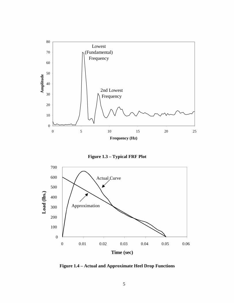
Frequency Response Function (FRF) – The resulting frequency domain curve
when an FFT is performed on a data curve showing the relative contributions of various
frequencies. Peaks represent the various modes of vibration. See Figure 1.3.
Heel Drop – An excitation function used to evaluate floors. The function, shown
in Figure 1.4, is defined as the force generated by a 170-lb. man, raised up on his toes
approximately two and one half inches, who shifts his weight to his heels as they strike
the floor. The actual curve is approximated by the straight-line ramp function shown.
Dynamic Loads – Loads applied over a finite period of time, or loads changing
with time, as opposed to static loads. See Figure 1.5.
e-β2πf
5
2nd Lowest Frequency
Lowest (Fundamental)
Frequency
0
10
20
30
40
50
60
70
80
0 5 10 15 20 25
Frequency (Hz)
Am
plit
ude
Figure 1.3 – Typical FRF Plot
0
100
200
300
400
500
600
700
0 0.01 0.02 0.03 0.04 0.05 0.06
Time (sec)
Loa
d (l
bs.)
Actual Curve
Approximation
Figure 1.4 – Actual and Approximate Heel Drop Functions

6
Figure 1.5 - Types of Dynamic Loads
(a) Harmonic Load (b)Periodic Load
(c) Transient Load (d) Impulsive Load
Period t

7
Mode Shape – The shape a structure assumes when it vibrates at a natural
frequency. See Figure 1.6
Figure 1.6 - Typical Beam and Floor System Mode Shapes
a) Beam
b) Floor System

8
1.4 BACKGROUND CRITERIA
Before this particular study is described in detail, it is important to review the
floor vibrations criteria historically used. This section briefly highlights the main points
of a number of criteria proposed and used over the years, starting with studies on human
perception of vibration.
Initial studies showed that human susceptibility to annoying floor vibrations is
dependent upon three factors: frequency, initial amplitude, and damping (Lenzen, 1969).
The basic element for determining the frequency of a floor system is the T-Beam model
shown in Figure 1.7 with the frequency of the T-Beam determined from:
EFFECTIVE WIDTH
SLAB DECK
EFFECTIVE WIDTH
btr
Figure 1.7 – T-Beam Model for It
357.1
WL
gEIf t
n = (1.1)
Here g = acceleration of gravity, E = modulus of elasticity, W = total weight supported
by the T-Beam, L = beam span.
Reiher and Meister (1931) conducted the first study that examined human
perception of vibration. They subjected a group of people to steady state vibrations and
asked them to rate the experience. From this data, a chart was created, called the Reiher-
Meister Scale, which was eventually applied to floor vibrations. In 1966, Lenzen
9
discovered that humans are much less sensitive to transient vibrations than they are to
steady state vibrations. He modified the Reiher-Meister Scale to reflect this and applied
his findings specifically to floor vibrations (Lenzen, 1966). In 1974, Wiss and Parmelee
studied the effect of transient vertical vibrations on a group of test subjects, using
frequency displacement and damping as parameters (Wiss and Parmelee, 1974). In 1975,
Murray introduced a design criterion that utilized a dynamic load factor to more
accurately predict the deflection of the system under a given load. Previous methods had
used a static analysis for determining deflection and predicted frequency based upon a
static load. Murray also introduced Dunkerly’s Equation to account for the fact that the
fundamental frequency of a floor system is a function of the fundamental frequency of
the beams and the girders, rather than just the beams, as had previously been assumed.
Dunkerly’s Equation is:
222
111
gbs fff+= (1.2)
Here fs = the system frequency, Hz; fb = the frequency of the beam, Hz; and fg = the
frequency of the girder, Hz (Murray, 1975). In 1976, Allen and Rainer introduced a
design criterion based on a number of walking tests performed on long span floors. This
criterion was included in the Canadian Standards Association Standard, CSA S16.1
(CSA, 1989). In 1981, Murray introduced a minimum required damping criterion that
was based on a series of tests. Floors were tested and were rated as either acceptable or
unacceptable. A line of best fit was then drawn through the data points and was used to
determine the minimum damping required in a system for the system to be acceptable
(Murray, 1981). In 1985, Wyatt introduced a design criterion for walking similar to the
current American Institute of Steel Construction (AISC) Design Guide procedure
(Murray, et al., 1997). In 1989, the International Organization for Standardization (ISO)
presented the scale shown in Figure 1.8. This scale, which shows the recommended

10
limits of peak acceleration, due to walking, for human tolerance, later became a core
portion of the AISC Design Guide procedure.
Frequency (Hz)
1 3 4 5 8 10 25 40
Peak
Acc
eler
atio
n (%
Gra
vity
)
0.1
0.050.05
0.25
0.5
1
2.5
5
10
25
Rhythmic Activities,Outdoor Footbridges
Indoor Footbridges,Shopping Malls,
Dining and Dancing
Offices,Residences
ISO Baseline Curve for RMS Acceleration
Limits Suggested by Allen and Murray
Figure 1.8 – Recommended Peak Acceleration for Human Tolerance

11
In 1990, Allen proposed a simplified model of the dynamic response of a floor
due to rhythmic loading. The basic model consisted of a person exerting a sinusoidal
force on a lumped mass attached to a spring and a damper. This simplification would
later form the basis for the portion of the AISC Design Guide that deals with the
acceleration response due to walking excitation. The derivation of the equation used by
Allen is included in Section 3.3.
All of the methods described here were based on the assumption that floor
vibrations are localized in a single bay. It is also assumed that the vibration
characteristics of a single bay are simply a function of the vibration characteristics of a T-
beam analysis for the beams and the girders in the bay. Finally, it is assumed that the T-
beam behaves as an equivalent single degree of freedom system with a particular
stiffness, damping ratio, and a lumped mass oscillating with only one mode of vibration.
The most current design criterion, AISC Design Guide 11, Floor Vibrations Due to
Human Activity, hereafter Design Guide, is also based on these same assumptions.
All of the methods previously surveyed are based on analyses of rectangular bays.
Since all bays are not necessarily rectangular, though, there is a need for an analysis
technique for evaluating more complex framing schemes. Two techniques were explored
for this study, and are presented in the following chapters. Since the Design Guide
method is the most current criterion available, it will be used for comparison purposes.
Section 1.5 is a detailed overview of the Design Guide procedure for walking excitation.
1.5 AISC DESIGN GUIDE 11
Allen and Murray (1993) proposed a criterion based on limits proposed by the
ISO shown previously in Figure 1.8, which later became the basis for the Design Guide
procedure. These limits take into account the fact that human tolerance for vibration
depends a great deal on the environment. For example, someone trying to study in a
library will tolerate far less vibration than someone shopping at a mall for Christmas
gifts.

12
The Design Guide method essentially requires two sets of calculations. First, it is
required to estimate the frequencies of the beams, the girders, and then the entire bay. In
general, it is assumed that the members are simply supported; however, cantilever
sections are considered. The second part is to estimate the peak acceleration due to
walking by estimating the effective mass of the system and then calculating the peak
acceleration due to a dynamic load of specific magnitude, oscillating at the lowest natural
frequency of the system, applied at an anti-node of the system.
Frequency. The fundamental frequency of a beam, Equation 1.3, is given in the
Design Guide as:
jj
gf
∆= 18.0 (1.3)
Here g = acceleration due to gravity and ∆j = deflection of the joist, beam, or girder under
the estimated loading. The maximum deflection of the beam occurs at mid-span and is
given as:
js
jjj IE
Lw
384
5 4
=∆ (1.4)
Here wj = weight per length of beam, Es = modulus of elasticity for steel, Ij = composite
moment of inertia, Lj = length of beam. (Note: Substitution of Equation 1.4 into Equation
1.3 yields Equation 1.1.) For hot-rolled sections, Ij is the fully composite moment of
inertia. However, for joists, Ij is the effective composite moment of inertia, which is
smaller than the fully composite moment of inertia since web shear deformations are
significant. For a joist, the effective composite moment of inertia is estimated from:
compchords
eff
II
I1
1
+= γ (1.5)

13
Here Ichords = moment of inertia of the bare steel, in.4; Icomp = fully composite moment of
inertia of the slab and the chords, in.4; and γ = a reduction factor given as:
11 −=
rCγ (1.6)
In Equation 1.6, Cr is a modification factor proposed by Band and Murray (1996) to
estimate the effective moment of inertia of a joist or joist-girder. Their study showed that
since the web members underwent significant shear deformation during loading, a
reduction in the effective moment of inertia was necessary. Equation 1.7 applies to joists
with angle web members, and Equation 1.8 applies to joists with rod webs. In each case,
L = length, in. and D = nominal depth, in.:
8.2)/(28.0 )1(90.0 DLr eC −−= for 6 ≤ L/D ≤ 24 (1.7)
)/(00725.0721.0 DLCr += for 10 ≤ L/D ≤ 24 (1.8)
For a girder, the calculations for frequency are the same, unless the girder
supports joists. To account for the fact that joist seats are not sufficiently stiff to justify
the use of the full composite moment of inertia, the following equation is used to
calculate the effective moment of inertia of the girder:
4/)( nccncg IIII −+= (1.9)
Here Inc = moment of inertia of the bare steel, in.4; Ic = fully composite moment of inertia,
in.4. In the case of a joist-girder, Inc is:
chordsrnc ICI = (1.10)
14
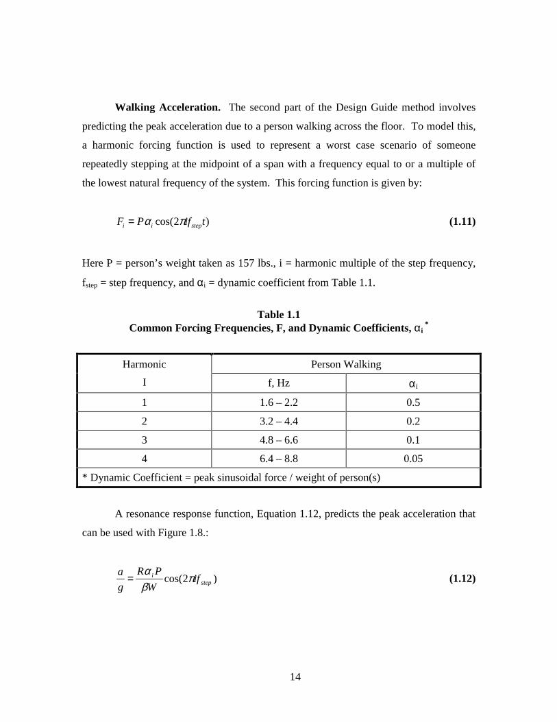
Walking Acceleration. The second part of the Design Guide method involves
predicting the peak acceleration due to a person walking across the floor. To model this,
a harmonic forcing function is used to represent a worst case scenario of someone
repeatedly stepping at the midpoint of a span with a frequency equal to or a multiple of
the lowest natural frequency of the system. This forcing function is given by:
)2cos( tifPF stepii πα= (1.11)
Here P = person’s weight taken as 157 lbs., i = harmonic multiple of the step frequency,
fstep = step frequency, and αi = dynamic coefficient from Table 1.1.
Table 1.1Common Forcing Frequencies, F, and Dynamic Coefficients, αi
*
Person WalkingHarmonic
I f, Hz αi
1 1.6 – 2.2 0.5
2 3.2 – 4.4 0.2
3 4.8 – 6.6 0.1
4 6.4 – 8.8 0.05
* Dynamic Coefficient = peak sinusoidal force / weight of person(s)
A resonance response function, Equation 1.12, predicts the peak acceleration that
can be used with Figure 1.8.:
)2cos( stepi if
W
PR
g
a πβα
= (1.12)

15
Here, /g = the ratio of the floor acceleration to the acceleration due to gravity, β = the
modal damping ratio, W = effective weight of the floor, and R = a reduction factor
recommended as 0.7 for footbridges and 0.5 for floor structures with two-way action.
For design, Equation 1.12 simplifies to (Allen and Murray, 1993):
W
fP
g
anop
β)35.0exp(−
= (1.13)
Here fn = natural frequency of the floor, Po = constant force equal to 65 lb. for floors and
92 lb. for footbridges, p/g = estimated peak acceleration, β = modal damping ratio, and
W = effective weight supported by the beam panel, girder panel, or combined panel, as
applicable, lbs. For entire floor systems, an effective panel weight for the beam is
combined with an effective panel weight for the girder to yield an effective panel weight
for the bay. In general, the effective weight of a panel is given as:
wBLW = (1.14)
Here L = member span, w = weight per unit area, B = effective width of the panel. For a
beam or joist panel, the effective width is given as:
jjsjj LDDCB 4/1)/(= (1.15)
Here, Ds = transformed slab moment of inertia per unit width, Dj = effective moment of
inertia of tee-beam per unit width, and Cj = 2 for most joists or beams and 1 for joists or
beams parallel to an interior edge. If the edge joist or beam is more than 50% stiffer than
the interior beams or joists, Cj should be taken as 2, even though it is an edge member.
For a girder, the effective width is:

16
ggjgg LDDCB 4/1)/(= (1.16)
Now, Cg = 1.6 for girders supporting joists connected to the girder flange, and 1.8 for
girders supporting beams connected to the girder web, and Dg = effective moment of
inertia per unit width. If the girder is an interior edge member, Bg should be taken as 2/3
of the supported beam or joist span.
For the combined mode, the effective panel weight is a function of the flexibility
of each member type and the effective weight of each panel type, and is given by:
ggj
gj
gj
j WWW∆+∆
∆+
∆+∆∆
= (1.17)
If a beam, joist, or girder is continuous over a support, and the adjacent span is at
least seven-tenths of the length of the center span, then the effective weight of that panel
may be increased by 50% to account for continuity. Hot-rolled shear connections are
acceptable here, but joists that are only connected at the top chord, and girders that frame
into a column, are excluded.
If the girder span is less that the effective width of the joist panel (Lg < Bj), the
combined mode is said to be restricted. In this case, the deflection of the girder is
multiplied by the factor in Inequality 1.18, subject to the limits shown:
0.15.0 ≤≤j
g
B
L(1.18)
This reduction applies to the calculation of W in Equation 1.17 and to the frequency of
the member, Equation 1.3.
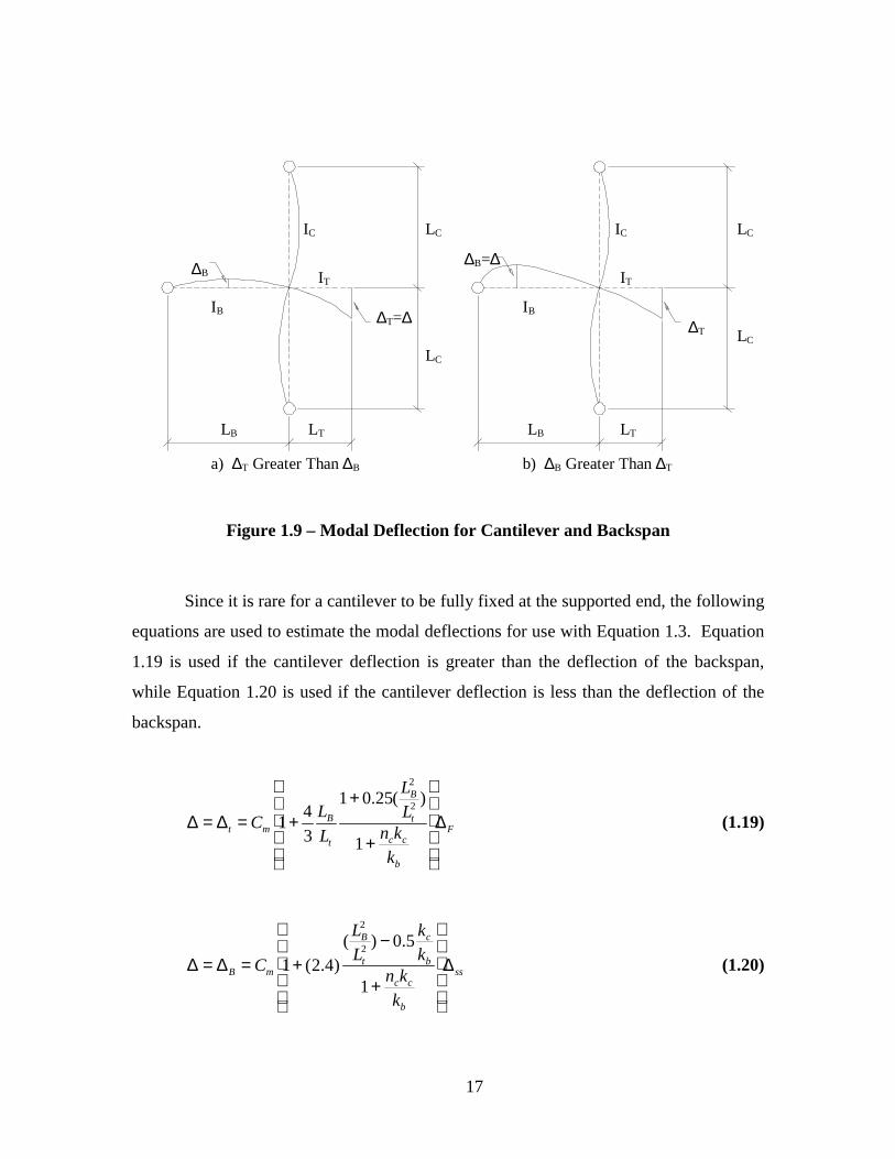
Cantilevers. For a cantilever member, the deflection at the tip of the cantilever is
most critical. Figure 1.9 defines some of the parameters used to estimate the deflection at
the tip of a cantilever.
17
∆T=∆ ∆T
∆B
IB
LB LT
a) ∆T Greater Than ∆B b) ∆B Greater Than ∆T
∆B=∆
IC
IT
IC
IB
IT
LB LT
LC
LC LC
LC
Figure 1.9 – Modal Deflection for Cantilever and Backspan
Since it is rare for a cantilever to be fully fixed at the supported end, the following
equations are used to estimate the modal deflections for use with Equation 1.3. Equation
1.19 is used if the cantilever deflection is greater than the deflection of the backspan,
while Equation 1.20 is used if the cantilever deflection is less than the deflection of the
backspan.
F
b
cc
t
B
t
Bmt
k
knL
L
L
LC ∆
+
++=∆=∆
1
)(25.01
3
41
2
2
(1.19)
ss
b
cc
b
c
t
B
mB
k
knk
k
L
L
C ∆
+
−+=∆=∆
1
5.0)()4.2(1
2
2
(1.20)

18
Here kb = IB/LB or the moment of inertia of the backspan divided by the length of
the backspan, kc = Ic/Lc is for the cantilever, Cm = 0.81 for a distributed mass and 1.06 for
a mass concentrated at the tip, nc = 2 for columns above and below, 1 for columns only
below, ∆f = deflection of a fully fixed cantilever under the weight supported, ∆ss =
deflection of the backspan assuming a simply supported member.
Acceptability Criterion. Once the peak acceleration response of the system is
estimated, it is compared to Inequality 1.21:
g
a
W
fP
g
aonop ≤
−=
β)35.0exp(
(1.21)
Here, o/g = limit of human tolerance as recommended by Murray and shown in Figure
1.8. For the case of office floors, o/g = 0.5%g.
1.6 OTHER CURRENT RESEARCH
Many other individuals have done research on the topic of floor vibrations, some
of which is directly related to the research presented in this paper. Kitterman (1994)
investigated the properties and behavior of steel joists and their impact on floor
vibrations. He developed several equations for calculating the effective moment of
inertia of a steel joist based on numerous test results and finite element models. Hanagan
(1994) explored the use of active control systems to reduce annoying floor vibrations.
Her research provided a known input and measured response for a multi-bay floor and is
referenced during the verification of the finite element modeling techniques. Band
(1996) researched joist and joist-girder supported floors and helped develop the reduction
factors used for calculating the effective moment of inertia of a joist. Rottmann (1996)
explored the use of tuned mass dampers for controlling floor vibrations. Beavers (1998)
used a finite element program to model single-bay joist-supported floors and predict
19
fundamental frequencies. He also developed the rigid-link elements and joist-seat
elements as well as several other modeling conventions used in this study.
1.7 NEED FOR RESEARCH
The wide variety of scales and prediction techniques available to engineers is an
indication of the complex nature of floor vibrations. Furthermore, since each method
inherently makes numerous assumptions about the structure, not all methods are equally
applicable to all situations. This study was done to evaluate the ability of two finite
element modeling techniques to predict both the fundamental frequency and the dynamic
response of a multi-bay floor, regardless of the regularity of beam spacing, material
properties, damping properties or other limitations. Current design standards are based
on regularly spaced rectangular bays that are approximated as a series of single degree of
freedom systems. Real structures, though, are far more complex. The results of the finite
element analyses are compared to current practices and field-measured results. Chapter
II discusses the finite element modeling techniques used in this study. The equipment
used and testing procedures for the floors are also discussed in Chapter II. In Chapter III
the computer models are verified by matching the results to closed form solutions and to
the predictions of the Design Guide method. Chapter IV summarizes the results of the
analyses performed on a number of in-situ floors. Each floor is described in detail, and
the results of both finite element modeling techniques are compared to results from the
Design Guide method and to various field measurements for each floor. In Chapter V,
conclusions are drawn and the need for more research is suggested. Appendix A contains
supporting data for the analyses presented in Chapter IV, while Appendix B contains a
detailed example of both finite element modeling techniques.
20
CHAPTER II
FINITE ELEMENT MODELING AND IN-SITU MEASURMENT TECHNIQUES
2.1 INTRODUCTION
To examine the ability of a finite element computer model to predict both the
fundamental frequency of a floor and the peak acceleration due to walking, two modeling
techniques were developed and test results were gathered. This chapter briefly describes
the finite element computer program used in this study, the 3D and 2D modeling
techniques developed, and the procedure and equipment used to take in-situ
measurements.
2.2 FINITE ELEMENT COMPUTER PROGRAM
2.2.1 OVERVIEW
For the purposes of this research, the commercial finite element program,
SAP2000 Nonlinear Version 7.1, hereafter SAP2000, from Computers and Structures,
Inc. (Wilson and Habibullah, 1998) was used. The program can perform static and
dynamic analyses of complex structures, including the effect of modal damping, while
running on a typical desktop computer. The program features a graphical interface that
makes the input of a structure and the interpretation of results quick and easy.
2.2.2 FINITE ELEMENTS USED
In this study, beam, shell, and plate finite elements were used. The beam element
used is referred to in SAP2000 as a three-dimensional frame element. The element is a
two-node beam element with three translational and three rotational degrees of freedom
at each end. In some cases, pre-defined sections were used, such as hot-rolled sections,
but in other instances the properties of the member had to be calculated and input

21
separately. Typically, each frame element was defined with the material properties of
steel, but occasionally, in the case of links and seats especially, another material was
used. Once a frame element was created, it could be used to define the properties of
elements in the model.
To model the concrete slab, plate or shell elements were used. Shell elements in
SAP2000 are four-node elements with six degrees of freedom at each node, and were
used for the 3D-FEMs. Plate elements in SAP2000 are also four-node elements, but they
allow only three degrees of freedom at each node and were used exclusively in the 2D-
FEMs. Both elements are defined in the same way as frame elements, and each element
can be assigned a set of material properties, usually concrete.
2.2.3 THREE DIMENSIONAL MODELING TECHNIQUE
Slab. Three-dimensional finite element models (3D-FEMs) were created using
frame and shell elements. The shell elements were used to represent the slab and were
placed at the centroid of the concrete above the ribs. The thickness of a typical shell
element was defined as the thickness of the slab above the ribs of the deck. This
assumption is typically made for beams, but is usually not considered to be valid for
girders. However, this study assumes that the assumption is valid for floors in general.
The concrete was defined as having a modulus of elasticity 1.35 times greater than the
modulus generally assumed for structural calculations. This was due to the fact that
concrete is stiffer under dynamic loading than it is under static loading (Allen and
Murray, 1993). The concrete was defined with a unit weight and unit mass given by:
)000,728,1
1)(
12)()
12
2/((
cldc
rc
dwww
ddW +++= (2.1)
386/WM = (2.2)
22
Here W = weight per unit volume, k/in3; dc = thickness of concrete above the ribs, in.; dr
= thickness of concrete in ribs, in.; wc = unit weight of concrete, pcf; wd = estimated
additional dead load on the floor, psf; wl = estimated additional live load on the floor, psf;
M = mass per unit volume, k-sec2/in4. This technique allowed for the fact that loading on
a real structure will inherently affect the natural frequencies of the structure by increasing
the total mass of the system. SAP2000 calculates frequencies based on the mass and
stiffness of the system independent of any loading on the structure. Therefore, to include
the effect of distributed loads, they must be included in the mass of the system.
Hot-Rolled Beams. Floors supported by hot-rolled sections were fairly simple to
model. Once the frame elements were defined for each section, they were drawn in the
finite element model at the location of their respective centroids. Since the members
were long and slender, the frame sections were modified so as to remove the effects of
shear deformations by setting the shear area equal to zero.
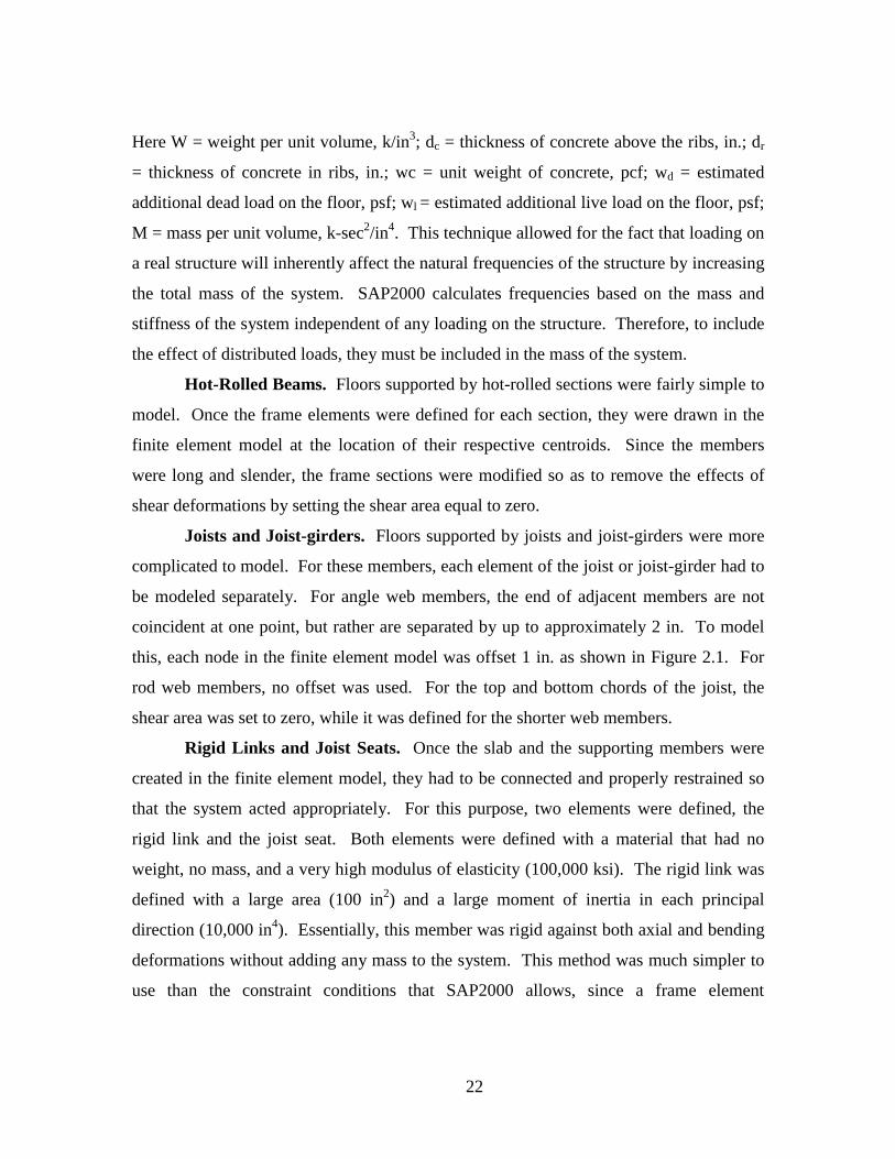
Joists and Joist-girders. Floors supported by joists and joist-girders were more
complicated to model. For these members, each element of the joist or joist-girder had to
be modeled separately. For angle web members, the end of adjacent members are not
coincident at one point, but rather are separated by up to approximately 2 in. To model
this, each node in the finite element model was offset 1 in. as shown in Figure 2.1. For
rod web members, no offset was used. For the top and bottom chords of the joist, the
shear area was set to zero, while it was defined for the shorter web members.
Rigid Links and Joist Seats. Once the slab and the supporting members were
created in the finite element model, they had to be connected and properly restrained so
that the system acted appropriately. For this purpose, two elements were defined, the
rigid link and the joist seat. Both elements were defined with a material that had no
weight, no mass, and a very high modulus of elasticity (100,000 ksi). The rigid link was
defined with a large area (100 in2) and a large moment of inertia in each principal
direction (10,000 in4). Essentially, this member was rigid against both axial and bending
deformations without adding any mass to the system. This method was much simpler to
use than the constraint conditions that SAP2000 allows, since a frame element

23
2” (approx.) 2”
a) Typical Joist Configuration b) Finite Element Model
Figure 2.1 - Definition of Joint Eccentricity
can easily be copied and multiplied. The use of the rigid link element with a hot rolled
beam is illustrated in Figure 2.2, while the use of the rigid link element with a joist is
illustrated in Figure 2.3. It is shown in Section 3.4 that these link elements develop the
composite action necessary.
The joist seat was defined with a large area (100 in2) and a near zero moment of
inertia in each principal direction (0.001 in4). Essentially, this member was rigid axially,
without providing any bending stiffness or additional mass to the system. This method
was also simpler than using the constraints provided in SAP2000, and it allowed for the
fact that joist seats are not sufficiently stiff to develop the fully composite moment of
inertia for the girder. The use of the seat element is illustrated in Figure 2.4.
Restraints and Releases. Once all of the elements were connected, the model was
restrained, and some joints were altered to accurately represent the actual floors.
Restraint was provided by the built-in joint restraints in SAP2000. Figure 2.5 shows the
restraints applied to a typical single bay floor assuming that the beams and the girders are
located in the same plane. For cases where the girder is deeper than the beams, the
restraints are applied at the ends of the girders only. One corner, in this case Corner 1,
was restrained in all three translational directions. The corner located at the other end of
the girder, in this case Corner 2, was restrained in the vertical direction (Z-direction) and
in the out-of plane direction (Y-direction). The diagonally opposite corner, in this case

24
SLAB CENTRO ID
RIGID LIN KS
BE AM CENTRO ID
Figure 2.2 – Rigid Links with Hot-Rolled Beams
SLAB CENTROID RIGID LINK
JOIST MEMBERS
Figure 2.3 – Rigid Links with Steel Joists
Slab
Joist Girder
Joist Seat
Bottom ChordFrame Element
Top ChordFrame Element
Seat Element
Shell Element
Rigid Link Element
Actual Joist SeatFinite Element Modelingof Joist Seat
Figure 2.4 – Joist Seats

25
Girder
GirderB
eam
1 2
43
a) Beam and Girder Restraints b) Slab Restraints
3 4
21 Meshed Slab
X
Y
Bea
m
Bea
m
Bea
m
Figure 2.5 – Typical Joint Restraints for 3D-FEM
Corner 4, was restrained from motion in the vertical direction and in the direction of the
girder (X-direction). All other column locations were restrained in the vertical (Z-
direction) only. For floors with joists or joists girders, all nodes along the bottom chord
were restrained from moving in the out of plane direction. The slab was also restrained
from movement in the plane of the slab. A corner not restrained on the girder level, in
this case, Corner 3, was restrained in both in-plane directions (X-direction and Y-
direction). The diagonally opposite corner, Corner 2, was restrained in one direction only
(X-direction).
Coincident joints in SAP2000 are assumed to be fully connected to one another.
However, when dealing with joists, continuity over a girder cannot be assumed if only the
top chord of the joist is connected to the top flange of the girder. For this reason, moment
releases were introduced at these locations. Moment releases were not used when hot-
26
rolled beams were connected to hot-rolled girders or when hot-rolled girders were
connected to columns, and moment releases were not introduced in the slab.
2.2.4 TWO DIMENSIONAL FINITE ELEMENT MODELING TECHNIQUE
Slab. Two-dimensional finite element models (2D-FEM) were created using
frame and plate elements. The plate elements were used to represent the slab. The
thickness of a typical plate element was defined as the thickness of the slab above the ribs
of the deck as was done in Section 2.2.3 for the 3D-FEM. The concrete was defined with
the dynamic modulus of elasticity and with a unit mass and unit weight which included
the concrete above the ribs, the concrete in the ribs, and any additional dead or live load
that was uniformly applied to the structure. This technique allowed for the fact that
loading on the structure will inherently affect the natural frequencies of the structure.
SAP2000 calculates frequencies based on the mass and stiffness of the system,
independent of any applied loading. Therefore, the additional loading was included as a
distributed mass rather than as a distributed load. The plate element was placed in a plane
located at the centroid of the concrete above the ribs.
Hot-Rolled Beams. For floors supported by hot-rolled sections, the composite
moment of inertia was calculated for each section and then the appropriate frame
elements were placed in the finite element model in the same plane as the slab. To avoid
counting the moment of inertia of the slab twice, the moment of inertia of the slab about
its centroid was subtracted from the composite moment of inertia used to define the frame
elements. Again, since the members were long and slender, the frame sections were
modified so as to remove the effects of shear deformations by setting the shear area equal
to zero.
Joists and Joist-Girders. Floors supported by joists and joist-girders were also
fairly simple to model in the 2D-FEM. Similar to the hot-rolled sections, the frame
members representing joists were defined with the effective moment of inertia from
Equation 1.5. For either joist-girders or hot-rolled sections supporting joists, Equation
1.9 was used to calculate the effective moment of inertia. All frame elements were

27
placed in the same plane as the plate elements representing the slab. Like the hot-rolled
sections, the shear area was set equal to zero in2 since shear deformations were already
accounted for in the inertia calculations.
Rigid Links and Joist Seats. The 2D-FEM did not require the use of links or
seats. The links were not needed since SAP2000 automatically connects coincident
joints, and all joints in the 2D-FEM are in the same plane. The seats were not required
because their effect was taken into account when the effective moment of inertia was
determined for the girders (Equation 1.9).
Restraints and Releases. Once all of the elements were connected, the model
was restrained, and some joints were altered to represent the actual floors. Restraint was
provided by the built-in joint restraints in SAP2000. Typically, 2D-FEMs were
restrained in the same manner as the slab in a 3D-FEM with the exception that all column
locations also received a vertical support.
Coincident joints in SAP2000 are assumed to be fully connected to one another.
However, when dealing with joists, continuity over a girder cannot be assumed if only the
top chords of the joist are connected to the top flange of the girder. For this reason,
moment releases were introduced at these locations. Moment releases were not used
when hot-rolled beams were connected to hot-rolled girders, and moment releases were
not introduced in the slab.
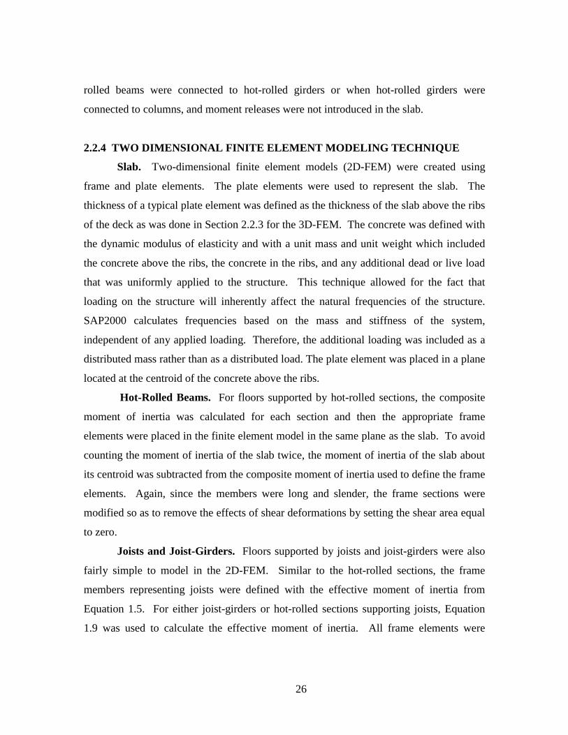
2.2.5 LOADING PROTOCOL AND TIME-HISTORY ANALYSES.
Once the model was created, three different static loads were applied. The first
load applied was simply the dead weight of the structure. This was used to check
deflections and the total mass of the system. The second load was a single, concentrated,
600-lb. point load, which is used for the heel drop analysis. The third load was a single,
concentrated load with magnitude equal to the magnitude of the walking load used in the
Design Guide. Allen (1990) showed that a point load oscillating at a natural frequency of
a system would give the same response as predicted by Equation 1.13. The magnitude of
the point load is:
28
nfeP 35.065 −= (2.3)
Two dynamic analyses were performed for each floor. A heel drop analysis was
completed using the static load for the heel drop case and a time history function. The
function consisted of a 50ms ramp function that started at 1 and decreased to 0, see
Figure 1.4. The analysis used the modal damping ratio that was estimated by the
measurement team. A walking analysis was completed using the static load for the
walking case and a time history function. Here, the function was a sine function that
oscillated at the natural frequency of the system. Again, the analysis used the modal
damping ratio estimated by the measurement team.
2.3 IN-SITU MEASURMENTS
Results from the Design Guide Procedure and the two finite element modeling
techniques were compared to one another and to data from the actual floor. A variety of
different tests was conducted for each floor, which measured the response of the floor to
different types of loading. In addition, a subjective evaluation was made for each floor.
Testing Equipment. To measure both the fundamental frequency of a floor and
the peak acceleration response of the floor, a series of tests was performed. The data was
collected with an Ono Sokki CF-1200 Handheld FFT Analyzer. The analyzer was
connected to a seismic accelerometer, manufactured by PCB Piezotronics as model 393C.
For each test, the acceleration was measured by the accelerometer and recorded on a data
card in the analyzer. The analyzer then performed a Fast Fourier Transform on the data
and created an FRF that was also stored as a second record on the data card. Once this
was completed, the next test could be run.
Floor Excitations. For each floor, as many as six possible excitations were
recorded. Not all excitations were recorded for all floors. Generally, the accelerometer
was placed as near to the center of the bay as possible since that is the location of
29
maximum response, and the test was performed close to the accelerometer. Generally,
ambient vibration of the floor was measured first. For this test, the measurement team
simply recorded the ambient vibration in the building at the time of testing, from which
the fundamental frequency of the floor framing was determined. The second type of
excitation was the aforementioned heel drop. For this test, a member of the measurement
team raised up on his toes approximately 2.5 in. and then shifted all of his weight to his
heels and impacted the floor. The third and fourth types of excitation were due to
walking. Here, a member of the measurement team walked across the floor parallel to the
direction of the beams and then perpendicular to the direction of the beams, each time
passing near the accelerometer. The fifth and sixth types of excitation involve resonance
with the first or second harmonic of the system, as described by Allen (1990). He found
that if the fundamental frequency of a system is the first or second harmonic of the
forcing frequency of a periodic input, then the input will adequately excite the
fundamental frequency of the floor. The actual input will not be a pure sine function, but
will rather be a function that is made up of a number of different frequencies. The
forcing input can then be written as a Fourier series, and it will be found that the second
or third term in the series will act in resonance with the fundamental frequency of the
floor. The fifth type of excitation, therefore, was walking in place. Here, a member of
the measurement team walked in place, near the accelerometer, at a pacing frequency that
was approximately one-half or one-third of the lowest natural frequency of the floor. The
sixth type of excitation was due to bouncing or rhythmic excitation. Here, a member of
the measurement team bounced in place at a slowly increasing frequency until harmonic
resonance with the lowest floor frequency was achieved.
Subjective Evaluations. In addition to the quantitative measurements taken
during a test of a floor, qualitative measurements were recorded as well. Members of the
measurement team were generally asked to give their impression of the acceptability of
the floor under a walking load and were asked to indicate how noticeable the vibrations
were. In addition, for floors that were in use at or near the time measurements were
taken, the occupants of the building gave a subjective evaluation.
30
CHAPTER III
VERIFICATION OF FINITE ELEMENT MODELING TECHNIQUES
3.1 INTRODUCTION
This chapter outlines the process of verifying the modeling techniques before
applying them to actual floors. Simple structural dynamics of a beam, a continuous
beam, a cantilevered section, and a beam-girder system are looked at first. Next, the
loading function used to represent walking is verified. Then an example from the Design
Guide is modeled to demonstrate that the rigid link elements used are acceptable. Next, a
single bay floor, supported by joists and joist-girders, is analyzed. Finally, a floor model
is presented representing an actual floor for which experimental data was previously
recorded. This is the only multi-bay model used for verification, and the only model for
which the actual dynamic response of the structure is known. Multi-bay floor models are
largely absent from the literature, as the prevailing assumption is that a single bay
accurately represents the behavior of the floor. Dynamic response of a structure due to a
known or assumed dynamic load is also largely absent from the literature, and so cannot
be used for verification here.
3.2 COMPARISON WITH THE DYNAMICS OF SIMPLE STRUCTURES
This section examines the ability of the proposed 3D and 2D modeling techniques
to match the dynamic response of several different members. In all cases, the closed
form solution in Biggs (1964) is used for comparison. Results for a simply supported
beam, a cantilever, and a continuous beam are presented for both modeling techniques,
and the results for a beam-girder system are presented for the 2D technique only.

31
3.2.1 SIMPLY SUPPORTED BEAM
For a simply supported beam of length, L, constant EI, and a particular mass
intensity, with a concentrated dynamic load, Biggs (1964) provides the following closed
form solutions for frequency and total deflection:
m
EI
l
nf n 2
2
2
π= (3.1)
)(sin)(sin4
12),(
22 l
xnDLF
l
cn
fml
Ftxy
nn
n
πππ∑= (3.2)
Here n = integer mode number, F = magnitude of the load, x = location along the
member, y(x,t)= displacement of member at location, x, and time, t, c = location of load,
DLF = dynamic load factor for the loading function, and fn = frequency, Hz.
Choosing the W12X40 beam shown in Figure 3.1, with a 6 ft wide concrete slab,
the dynamic load shown in Figure 3.2, and its associated DLF, Equation 3.3, the first
fundamental mode of vibration is calculated:
Load, F
6’ - 0" 9’ - 0"
3"
6’ - 0"
W12X40
F = 1000 lbs. Icomp = 807 in4
Concrete: wc = 145 pcf, f’c = 3 ksi, dc = 3 ”
Figure 3.1 – Simply Supported Beam
32
F
t, sectd = 0.1
Force,lb
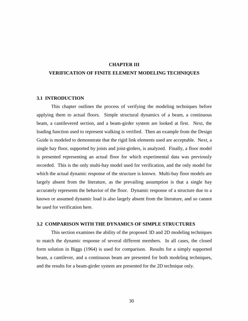
Figure 3.2 – Ramp Function for Dynamic Load
ddn
nnn t
t
t
ttDLF −+−=
ωωω sin
cos1 (for t < td) (3.3)
(Note: sometimes, but not here, frequency is presented as an angular frequency,
ωn, with units of radians per second.)
From the values assigned to the beam, the transformed concrete width is
calculated as 10.14 in., yielding a composite moment of inertia of 807 in4. Using this
information with Equations 3.1 and 3.2, and then differentiating Equation 3.2 twice, the
frequency, displacement, velocity and acceleration at mid-span are calculated. The
values for the closed form solution are compared to the values predicted by the finite
element models in Table 3.1. Clearly, the finite element modeling techniques give
excellent results for frequency, deflection, velocity, and acceleration in this case. The
3D-FEM gives slightly different results because the effective moment of inertia
calculated is slightly less than the full composite moment of inertia which is assumed for
the 2D-FEM and the closed form solution.
33
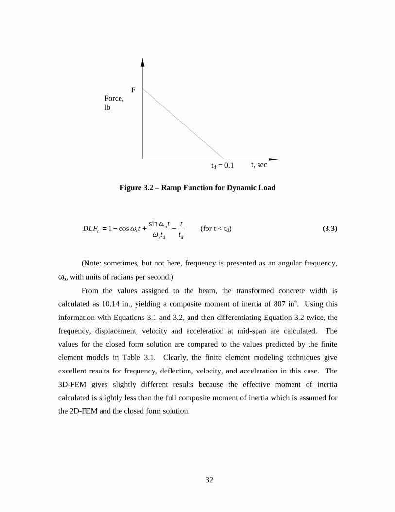
Table 3.1Simply Supported Beam Results
Biggs 3D-FEM 2D-FEM
Natural Frequency (ωn/2π) 31.4 Hz 30.4 Hz 31.4 Hz
Maximum Deflection 0.014 in 0.015 in 0.014 in
Minimum Deflection -0.027 in -0.028 in -0.027 in
Maximum Velocity 3.03 in/s 3.07 in/s 3.02 in/s
Minimum Velocity -2.74 in/s -2.77 in/s -2.72 in/s
Maximum Acceleration 570 in/s2 557 in/s2 567 in/s2
Minimum Acceleration -570 in/s2 -558 in/s2 -567 in/s2
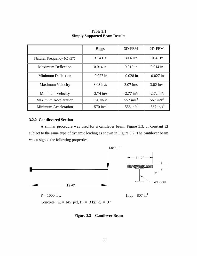
3.2.2 Cantilevered Section
A similar procedure was used for a cantilever beam, Figure 3.3, of constant EI
subject to the same type of dynamic loading as shown in Figure 3.2. The cantilever beam
was assigned the following properties:
Load, F
12’-0"
6’ - 0"
W12X40
3"
F = 1000 lbs. Icomp = 807 in4
Concrete: wc = 145 pcf, f’c = 3 ksi, dc = 3 ”
Figure 3.3 – Cantilever Beam

34
From these values, the transformed concrete width is calculated as 10.14 in.,
yielding a composite moment of inertia of 807 in4. For the primary mode of vibration,
the fundamental frequency is given by Equation 3.4, and the deflection at the tip is given
by Equation 3.5:
m
EI
ln 2
2)597.0( πω = (3.4)
]sin
cos1[4
),(2
ddn
nn
n t
t
t
tt
ml
Ftly −+−=
ωωω
ω(3.5)
Table 3.2 compares the results of the closed form solution (Biggs, 1964) to that
obtained from the finite element models. Again, there is excellent correlation.
Table 3.2Cantilever Beam Results
Biggs 3D-FEM 2D-FEM
Natural Frequency (ωn/2π) 17.5 Hz 17.3 Hz 17.5 Hz
Maximum Deflection 0.071 in 0.073 in 0.070 in
Minimum Deflection -0.210 in -0.220 in -0.210 in
Maximum Velocity 14.9 in/s 14.9 in/s 14.9 in/s
Minimum Velocity -12.4 in/s -12.4 in/s -12.4 in/s
Maximum Acceleration 1504 in/s2 1481 in/s2 1500 in/s2
Minimum Acceleration -1504 in/s2 -1481 in/s2 -1499 in/s2
35
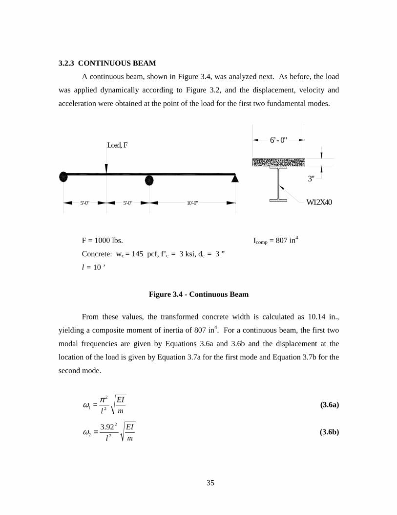
3.2.3 CONTINUOUS BEAM
A continuous beam, shown in Figure 3.4, was analyzed next. As before, the load
was applied dynamically according to Figure 3.2, and the displacement, velocity and
acceleration were obtained at the point of the load for the first two fundamental modes.
Load, F
5’-0" 5’-0" 10’-0"
6’ - 0"
W12X40
3"
F = 1000 lbs. Icomp = 807 in4
Concrete: wc = 145 pcf, f’c = 3 ksi, dc = 3 ”
l = 10 ’
Figure 3.4 - Continuous Beam
From these values, the transformed concrete width is calculated as 10.14 in.,
yielding a composite moment of inertia of 807 in4. For a continuous beam, the first two
modal frequencies are given by Equations 3.6a and 3.6b and the displacement at the
location of the load is given by Equation 3.7a for the first mode and Equation 3.7b for the
second mode.
m
EI
l 2
2
1
πω = (3.6a)
m
EI
l 2
2
2
92.3=ω (3.6b)
36
]sin
cos1[),(1
112
1 dd t
t
t
tt
ml
Ftly −+−=
ωωω
ω (3.7a)
]sin
cos1[),(2
222
2 dd t
t
t
tt
ml
Ftly −+−=
ωωω
ω (3.7b)
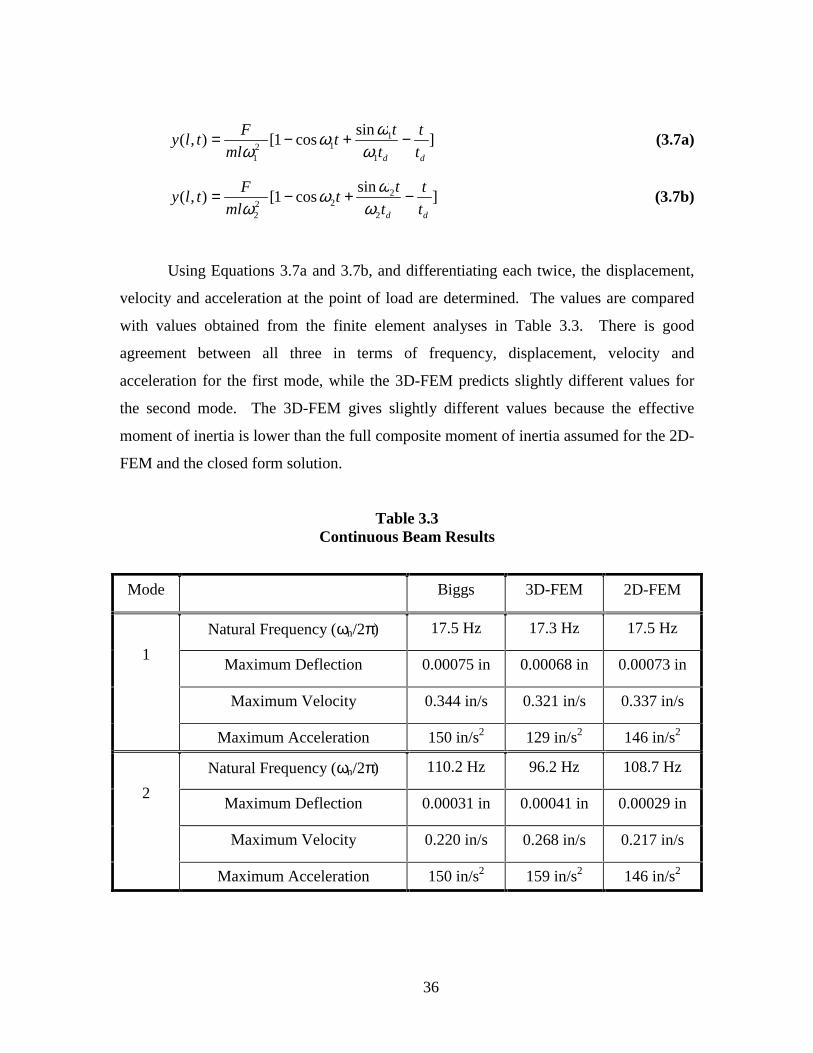
Using Equations 3.7a and 3.7b, and differentiating each twice, the displacement,
velocity and acceleration at the point of load are determined. The values are compared
with values obtained from the finite element analyses in Table 3.3. There is good
agreement between all three in terms of frequency, displacement, velocity and
acceleration for the first mode, while the 3D-FEM predicts slightly different values for
the second mode. The 3D-FEM gives slightly different values because the effective
moment of inertia is lower than the full composite moment of inertia assumed for the 2D-
FEM and the closed form solution.
Table 3.3Continuous Beam Results
Mode Biggs 3D-FEM 2D-FEM
Natural Frequency (ωn/2π) 17.5 Hz 17.3 Hz 17.5 Hz
Maximum Deflection 0.00075 in 0.00068 in 0.00073 in
Maximum Velocity 0.344 in/s 0.321 in/s 0.337 in/s
1
Maximum Acceleration 150 in/s2 129 in/s2 146 in/s2
Natural Frequency (ωn/2π) 110.2 Hz 96.2 Hz 108.7 Hz
Maximum Deflection 0.00031 in 0.00041 in 0.00029 in
Maximum Velocity 0.220 in/s 0.268 in/s 0.217 in/s
2
Maximum Acceleration 150 in/s2 159 in/s2 146 in/s2
37
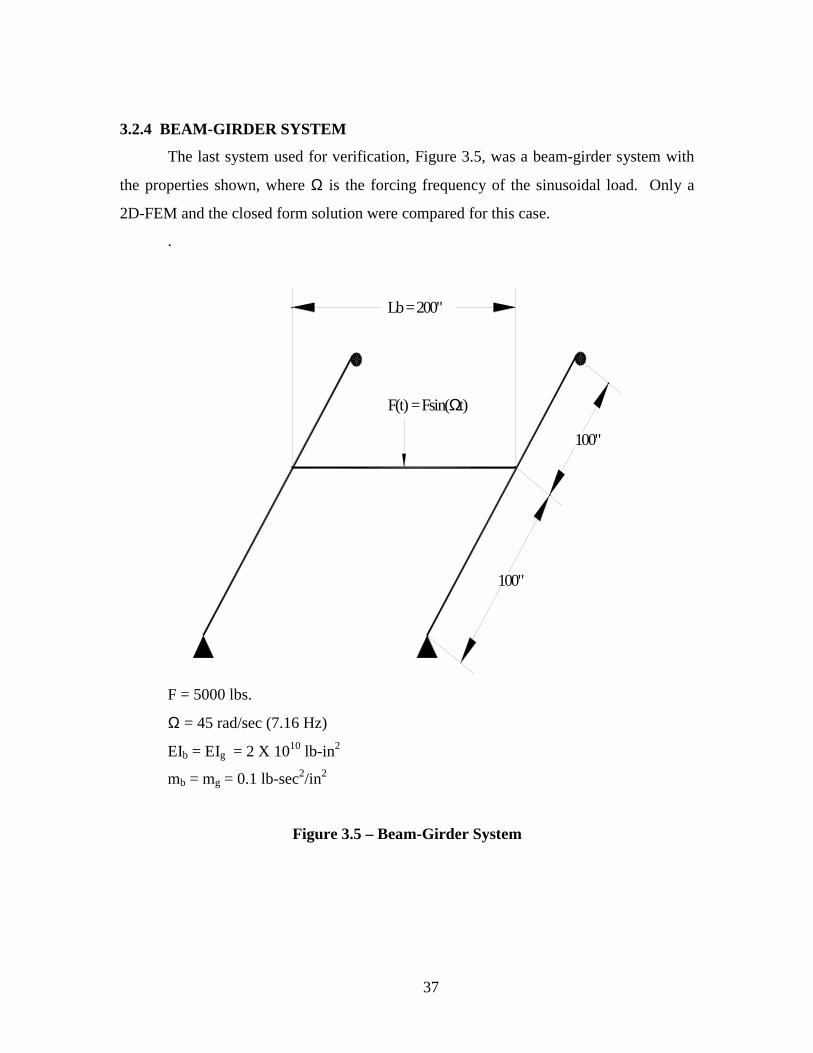
3.2.4 BEAM-GIRDER SYSTEM
The last system used for verification, Figure 3.5, was a beam-girder system with
the properties shown, where Ω is the forcing frequency of the sinusoidal load. Only a
2D-FEM and the closed form solution were compared for this case.
.
Lb = 200"
100"
100"
F(t) = Fsin(Ωt)
F = 5000 lbs.
Ω = 45 rad/sec (7.16 Hz)
EIb = EIg = 2 X 10¹⁰ lb-in2
mb = mg = 0.1 lb-sec2/in2
Figure 3.5 – Beam-Girder System

38
Using LaGrange’s equations and the energy method, the kinetic energy and the
strain energy of the system are calculated, assuming that each member vibrates in the
fundamental bending mode of a simply supported beam, yielding a 2 degree of freedom
system. From these results, the equations of motion are found, as is the determinant of
the 2X2 coefficient matrix, which leads to the fundamental frequencies of the system.
From these, the maximum deflection is found for the beam, the girders, and the system in
total (Biggs, 1964). The results are shown in Table 3.4, along with the results from the
finite element analysis. Clearly, the results from the finite element model are in good
agreement with the closed form solution.
Table 3.4Beam/Girder System Results
Mode Biggs 2D-FEM
Natural Frequency (ωn/2π) 11.1 Hz 11.0 Hz
Max. Deflection of Girder 0.048 in. 0.048 in.1
Max. Deflection of Beam 0.088 in. 0.088 in.
Natural Frequency (ωn/2π) 25.6 Hz 25.5 Hz
Max. Deflection of Girder -0.00803 in. -0.00803 in.2
Max. Deflection of Beam 0.0112 in. 0.0115 in.
Max. Deflection of Girder 0.04 in. 0.04 in.Combined
Max. Deflection of Beam 0.099 in. 0.010 in.
3.3 DESIGN GUIDE WALKING LOAD
According to the Design Guide, the peak acceleration of a floor due to a person of
average weight walking across the middle of the floor in harmony with the fundamental
frequency of the floor is given as:
W
fP
g
anop
β)35.0exp(−
= (3.8)

39
To use the finite element techniques, it was necessary to determine the load that
would need to be applied to the model to match this prediction. The standard solution for
a single degree of freedom system under a sinusoidal load is given by Allen (1990) as:
222 )/2(])/(1[
)2sin(
nn ffff
ft
k
Px
βφπ
+−
−= (3.9)
Here P = magnitude of load, k = stiffness, f = forcing frequency, fn = natural frequency,
β=damping ratio, φ = phase angle between the load and the response of the structure.
Taking two derivatives and setting the forcing frequency equal to the natural frequency,
the acceleration response is equal to:
βπ
M
ftPa p 2
)2sin(= (3.10)
Here M = mass of the system. Dividing by the acceleration due to gravity and noting that
the equivalent mass of a simply supported beam represented as a single degree of
freedom system is equal to 50% of the actual mass, the previous equation reduces to:
βπ
W
ftPga p
)2sin(/ = (3.11)
It follows then that the maximum acceleration, if f = fn, is:
βW
Pga p =/ (3.12)
Therefore, to obtain the same response in the finite element model as required in
the Design Guide procedure, the static load applied, P, must have a magnitude equal to

40
Poexp(-0.35fn) and be applied as a harmonic load with a forcing frequency equal to the
natural frequency of the system.
3.4 DESIGN GUIDE FOOTBRIDGE EXAMPLE
The next step in the verification of the finite element modeling technique is to
model a simple footbridge and compare the results obtained from both 3D-FEMs and the
2D-FEM to those provided in Chapter IV of the Design Guide. For this purpose,
Example 4.2 of the AISC Design Guide is used.
Footbridge Description. The footbridge is shown in Figure 3.6:
W 21 X 44
6"
10’
Concrete: wc = 145 pcf, f’c = 4000 psi
Slab + deck weight = 75 psf
Beams: W 21 X 44, A = 13.0 in.2, I = 843 in.4, d = 20.66 in.
Span: L = 40 ft
Icomp = 5,818 in4
Figure 3.6 – Footbridge Cross Section
Design Guide Procedure. Using the dynamic modulus of elasticity for the
concrete, the information provided, and the equations given in Chapter I, the natural
frequency of the footbridge is found to be 6.6 Hz. Assuming a damping ratio of 0.01 for
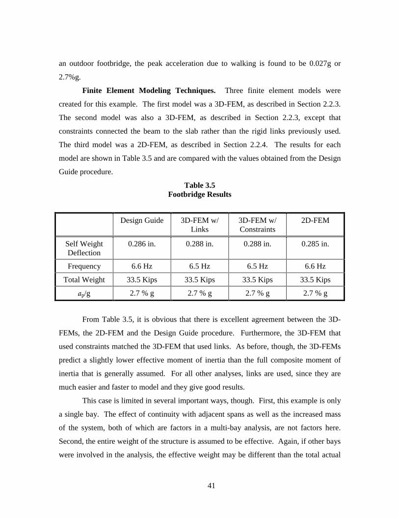
41
an outdoor footbridge, the peak acceleration due to walking is found to be 0.027g or
2.7%g.
Finite Element Modeling Techniques. Three finite element models were
created for this example. The first model was a 3D-FEM, as described in Section 2.2.3.
The second model was also a 3D-FEM, as described in Section 2.2.3, except that
constraints connected the beam to the slab rather than the rigid links previously used.
The third model was a 2D-FEM, as described in Section 2.2.4. The results for each
model are shown in Table 3.5 and are compared with the values obtained from the Design
Guide procedure.
Table 3.5Footbridge Results
Design Guide 3D-FEM w/Links
3D-FEM w/Constraints
2D-FEM
Self WeightDeflection
0.286 in. 0.288 in. 0.288 in. 0.285 in.
Frequency 6.6 Hz 6.5 Hz 6.5 Hz 6.6 Hz
Total Weight 33.5 Kips 33.5 Kips 33.5 Kips 33.5 Kips
p/g 2.7 % g 2.7 % g 2.7 % g 2.7 % g
From Table 3.5, it is obvious that there is excellent agreement between the 3D-
FEMs, the 2D-FEM and the Design Guide procedure. Furthermore, the 3D-FEM that
used constraints matched the 3D-FEM that used links. As before, though, the 3D-FEMs
predict a slightly lower effective moment of inertia than the full composite moment of
inertia that is generally assumed. For all other analyses, links are used, since they are
much easier and faster to model and they give good results.
This case is limited in several important ways, though. First, this example is only
a single bay. The effect of continuity with adjacent spans as well as the increased mass
of the system, both of which are factors in a multi-bay analysis, are not factors here.
Second, the entire weight of the structure is assumed to be effective. Again, if other bays
were involved in the analysis, the effective weight may be different than the total actual
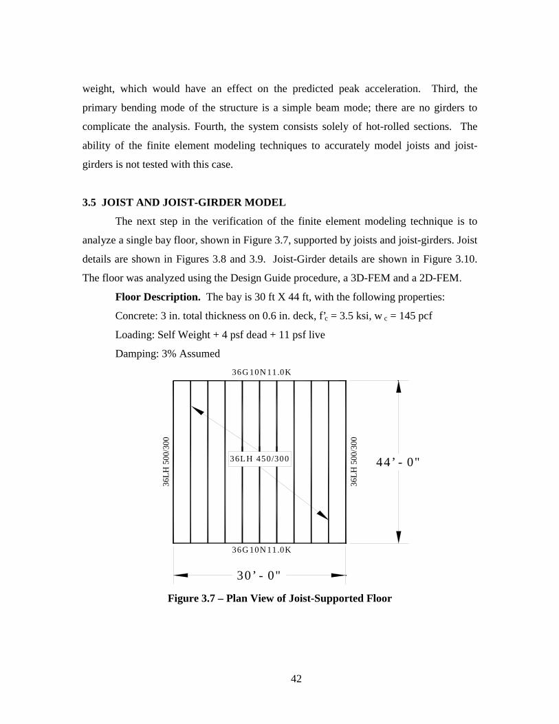
42
weight, which would have an effect on the predicted peak acceleration. Third, the
primary bending mode of the structure is a simple beam mode; there are no girders to
complicate the analysis. Fourth, the system consists solely of hot-rolled sections. The
ability of the finite element modeling techniques to accurately model joists and joist-
girders is not tested with this case.
3.5 JOIST AND JOIST-GIRDER MODEL
The next step in the verification of the finite element modeling technique is to
analyze a single bay floor, shown in Figure 3.7, supported by joists and joist-girders. Joist
details are shown in Figures 3.8 and 3.9. Joist-Girder details are shown in Figure 3.10.
The floor was analyzed using the Design Guide procedure, a 3D-FEM and a 2D-FEM.
Floor Description. The bay is 30 ft X 44 ft, with the following properties:
Concrete: 3 in. total thickness on 0.6 in. deck, f’c = 3.5 ksi, w c = 145 pcf
Loading: Self Weight + 4 psf dead + 11 psf live
Damping: 3% Assumed
36G 10N 11.0K
30 ’ - 0"
44 ’ - 0"36L H 450/300
36G 10N 11.0K
36L
H 5
00/3
00
36L
H 5
00/3
00
Figure 3.7 – Plan View of Joist-Supported Floor
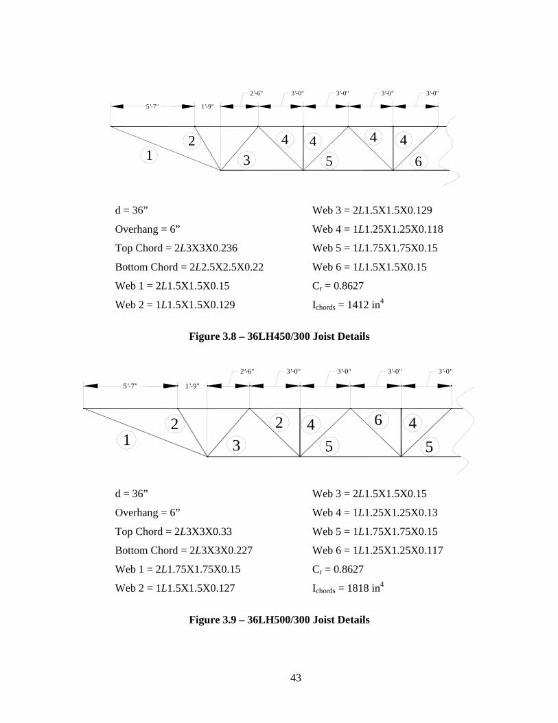
43
5’-7" 1’-9"
2’-6" 3’-0" 3’-0" 3’-0" 3’-0"
12
3
4 45
4 4
6
d = 36”
Overhang = 6”
Top Chord = 2L3X3X0.236
Bottom Chord = 2L2.5X2.5X0.22
Web 1 = 2L1.5X1.5X0.15
Web 2 = 1L1.5X1.5X0.129
Web 3 = 2L1.5X1.5X0.129
Web 4 = 1L1.25X1.25X0.118
Web 5 = 1L1.75X1.75X0.15
Web 6 = 1L1.5X1.5X0.15
Cr = 0.8627
Ichords = 1412 in4
Figure 3.8 – 36LH450/300 Joist Details
5’-7" 1’-9"
2’-6" 3’-0" 3’-0" 3’-0" 3’-0"
12
3
2 45
6 4
5
d = 36”
Overhang = 6”
Top Chord = 2L3X3X0.33
Bottom Chord = 2L3X3X0.227
Web 1 = 2L1.75X1.75X0.15
Web 2 = 1L1.5X1.5X0.127
Web 3 = 2L1.5X1.5X0.15
Web 4 = 1L1.25X1.25X0.13
Web 5 = 1L1.75X1.75X0.15
Web 6 = 1L1.25X1.25X0.117
Cr = 0.8627
Ichords = 1818 in4
Figure 3.9 – 36LH500/300 Joist Details

44
2’-7" 1’-9"
1’-3" 3’-0" 3’-0" 3’-0"
12
3
4 54
2 4
d = 36”
Overhang = 6”
Seat = 5”
Top Chord = 2L4X4X0.375
Bottom Chord = 2L4X4X0.375
Web 1 = 2L4X4X0.44
Web 2 = 2L1.5X1.5X0.15
Web 3 = 2L2.5X2.5X0.25
Web 4 = 2L2X2X0.176
Web 5 = 1L2X2X0.176
Cr = 0.7550
Ichords = 3270 in4
Figure 3.10 – 36G10N11.0K Joist-Girder Details
It is noted that the exterior joists are different than the interior joists. In the
Design Guide procedure, if the exterior member on a free edge is more than 50% stiffer
than the interior members, then the floor is not classified as a mezzanine, and Cj = 2.0 in
Equation 1.15. In this case, the edge joists are not 50% stiffer than the interior joists, and
the effect that this has on the finite element models will be examined.
Design Guide Procedure. Using the Design Guide procedure, outlined in
Chapter I, the moments of inertia for the interior joists and the joist-girders were
computed. The edge joists were not included in this procedure, since it was assumed that
the vibrations are a function of the interior joists and the joist-girders only. As noted
previously, the edges of the floor are free and the exterior joist is not more than 50%
stiffer than the interior joist, so the bay is classified as a mezzanine and Cj = 1.0 in
Equation 1.15. The results are presented in Table 3.6.
Finite Element Technique. Two finite element models were analyzed. A 3D-
FEM was analyzed using the procedure outlined in Section 2.2.3. Joist seats and rigid
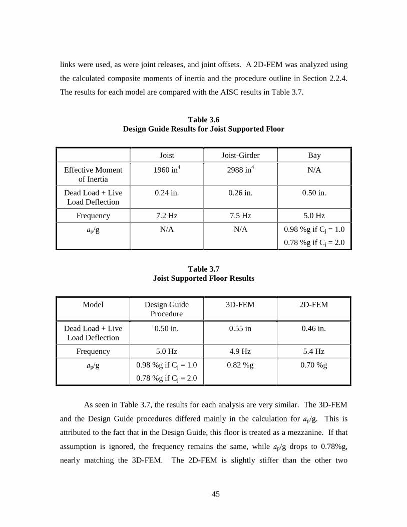
45
links were used, as were joint releases, and joint offsets. A 2D-FEM was analyzed using
the calculated composite moments of inertia and the procedure outline in Section 2.2.4.
The results for each model are compared with the AISC results in Table 3.7.
Table 3.6Design Guide Results for Joist Supported Floor
Joist Joist-Girder Bay
Effective Momentof Inertia
1960 in4 2988 in4 N/A
Dead Load + LiveLoad Deflection
0.24 in. 0.26 in. 0.50 in.
Frequency 7.2 Hz 7.5 Hz 5.0 Hz
p/g N/A N/A 0.98 %g if Cj = 1.0
0.78 %g if Cj = 2.0
Table 3.7Joist Supported Floor Results
Model Design GuideProcedure
3D-FEM 2D-FEM
Dead Load + LiveLoad Deflection
0.50 in. 0.55 in 0.46 in.
Frequency 5.0 Hz 4.9 Hz 5.4 Hz
p/g 0.98 %g if Cj = 1.0
0.78 %g if Cj = 2.0
0.82 %g 0.70 %g
As seen in Table 3.7, the results for each analysis are very similar. The 3D-FEM
and the Design Guide procedures differed mainly in the calculation for p/g. This is
attributed to the fact that in the Design Guide, this floor is treated as a mezzanine. If that
assumption is ignored, the frequency remains the same, while p/g drops to 0.78%g,
nearly matching the 3D-FEM. The 2D-FEM is slightly stiffer than the other two

46
analyses, as evidenced by the higher frequency and smaller deflection of the static
analysis.
3.6 MULTI-BAY FLOOR WITH DYNAMIC LOAD
The final step in the verification of the finite element modeling technique is a
comparison with a multi-bay floor where the frequency response and the dynamic
response to a specific load are both known. For this floor, the Design Guide procedure
was used only to predict a fundamental frequency, since the procedure can not predict the
dynamic response of the structure to the given load. A 3D-FEM was also constructed and
the results were compared to the measured response.
Description of Floor. This building is a multi-story laboratory located in
Vermont. The building footprint is an area 57 ft X 95 ft and consists of three bays in the
short direction and six bays in the long direction. Of the bays in the short direction, the
first is a laboratory spanning 21 ft 7 in., the second is a corridor spanning 7 ft and the
third is another laboratory spanning 28 ft 7 in. The larger of the two laboratories is where
testing occurred. In the long direction, the tested bay spans 18 ft, while the bays on either
side span 15 ft 1 in. The floor slab consists of 3 in. (total depth) of 4-ksi normal-weight
concrete supported by a 0.6-in. deck. The slab is supported on 16K7 and 16K2 joists,
spaced at 24 in. on center, with cross-sectional areas of 1.955 in2 and 1.069 in2 and
moments of inertia of the bare chords of 109 in4 and 59 in4 respectively. The joists rest
on hot-rolled beams, and the exterior edges of the slab are integral with the exterior wall.
A framing plan for a typical area of this building is shown in Figure 3.11.
The modal damping for this structure was measured as 4.5%. The loading on the
structure at the time of testing was estimated to consist of 3 psf of dead load and 5 psf of
live load, which includes island type workbenches where the intended function has been
impaired due to the annoying levels of vibration.
Design Guide Procedure. Using the given moments of inertia for the joists and
the estimated loading, the fundamental frequency of the floor was calculated as 7.13 Hz.

47
15’ - 1" 18’ - 0" 15’ - 1"
21’ - 7"
7’ - 0"
28’ - 7"
W 16 X 31
W 16 X 31
W 16 X 26
W 16 X 26 W 16 X 26
W 16 X 26
Exterior Wall
Exterior Wall
16K7 Joists @ 24" O. C.
16K2 Joists @ 24" O. C.
Figure 3.11 – Chemistry Laboratory Floor Plan
Measured Test Results. Hanagan (1994) presents the results of her
measurements of the floor. The fundamental natural frequency of the floor was measured
as 7.1 Hz. In addition to this, a series of heel drops was performed at the center of the
bay tested. The force input was recorded, as was the velocity response of the floor. The
input and output are shown in Figure 3.12.
Finite Element Results. A 3D-FEM was constructed according to the method
described in Section 2.2.3. As mentioned, the exterior girders were restrained to model
the fact that the slab was integral with the exterior walls at the edges. The frequency

48
Figure 3.12 – Measured Excitation and Response for Chemistry Laboratory
Time (sec)4 6 8 10 12 14 1620
Vel
ocit
y (i
n/se
c)
0.6
0.4
0.2
-0.6
-0.4
-0.2
0.0
Figure 3.13 – Dynamic Response of 3D-FEM to Series of Heel Drop Excitations
predicted by the model is 7.25 Hz. Additionally, a series of theoretical heel drops were
applied at the center of the tested bay to represent the loading applied to the actual
structure. The dynamic response of the 3D-FEM is shown in Figure 3.13. Clearly, both

49
the predicted frequency and dynamic response of the structure closely match the
measured results reported by Hanagan (1994).
3.7 CONCLUSION
In general, the finite element modeling technique provides excellent results for
this portion of the study. Natural frequencies and dynamic responses were in good
agreement between closed form solutions, the Design Guide method, and the finite
element technique. However, due to limitations in the literature, only rather simple
systems could be verified. Even the multi-bay floor, for which test results existed, was
fairly simple, since the narrow corridor in the middle acts to stiffen the system and to
isolate the exterior bays. In this way, even a multi-bay floor behaves as a single bay. In
Chapter IV the results for more complicated framing schemes of multi-bay floors are
given.
50
CHAPTER IV
DESCRIPTION OF TEST CASES AND COMPARISON OF RESULTS
4.1 INTRODUCTION
Once the finite element modeling techniques were verified, they were used to
analyze a number of floors. The floors studied are more complicated than other floors
found in the literature, since they are not limited to a single bay, as most other research is.
The floors examined included joist and hot-rolled beam-supported floors, as well as
floors with joist-girders. Both light weight and normal weight concrete was used, as were
a variety of loads and damping ratios. Some floors were constructed in the laboratory,
while others were actual floors currently in use across the United States. This chapter
presents a brief description of each floor, summarizes the results of the Design Guide
predictions and the finite element analyses, both 3D-FEMs and 2D-FEMs, and compares
these results to the field measurements taken at each site. Before discussing each floor in
detail, some general comments are presented here.
Frequency Response Function. For each floor, several FRFs are presented in
Appendix A. A sample experimental FRF is shown in Figure 4.1. The first and second
peaks are labeled as the first and second vibration frequencies, respectively. Generally, at
least three FRFs are shown in Appendix A, one for the 3D-FEM, one for the 2D-FEM,
and one for the measured experimental response, for each floor. In some cases, a fourth
FRF is shown, corresponding to a special case. The FRFs from the 3D-FEM and 2D-
FEM are generated using a spreadsheet program. The acceleration response from a heel
drop load is saved as a text file, imported into a spreadsheet, and a Fourier Analysis is
performed. The resolution of the FRF is a function of the number of data points stored
and the length of the time history analysis. For these cases, 4096 data points were stored

51
over a 4 second time period, corresponding to a frequency resolution of 0.25 Hz. This
was chosen because it matches the resolution of the handheld analyzer used for all
experimental measurements. It is noted that the absolute value of each peak has very
little significance; only the relative magnitude of each peak is important.
2nd Lowest Frequency
Lowest (Fundamental)
Frequency
0
10
20
30
40
50
60
70
80
0 5 10 15 20 25
Frequency (Hz)
Am
plit
ude
Figure 4.1 – Sample FRF
Acceleration. For each FEM analysis, the peak acceleration due to walking was also
recorded. A sample acceleration trace predicted by a 3D-FEM is shown in Figure 4.2.
The acceleration traces for each FEM are essentially identical, except for their magnitude,
because in each case the system reaches a steady-state condition. Therefore, the
acceleration traces are not included in Appendix A, rather the peak value is simply
reported for each floor.
Measured acceleration responses are shown in Appendix A for each floor tested.
Each acceleration response corresponds to one of the six excitations described in Section
2.3.

52
-0.5
-0.4
-0.3
-0.2
-0.1
0
0.1
0.2
0.3
0.4
0.5
0 1 2 3 4
TIME (s)
AC
CE
LE
RA
TIO
N (
%g)
Figure 4.2 – Sample Acceleration Trace From a 3D-FEM
A detailed description of each floor and a summary of the results are presented in the
following sections.
4.2 BUILDING 1
Building 1, constructed in 1998, is a three-story office building. The building
footprint is an area 120 ft X 182 ft and consists of three bays in the short direction and six
bays in the long direction. The outside bays in the long direction are relatively open with
no permanent partitions, but they do contain a large number of closely spaced
demountable partitions. The interior bays contain full height partitions; the business
environment is categorized as a “paper” office, with about 3% modal damping. The floor
slab consists of 5-5/8 in. (total depth) of 4-ksi lightweight concrete supported by a 3 in.
deck. A detailed framing plan for a typical area of this building is shown in Figure 4.3.

53
30’-
0"30
’-0"
30’-
0"
W 21X44
W 21X44
W 21X44
W 21X44
W 21X44
W 21X44
W 21X44
W 21X44
W 21X44
W 21X44
W 21X44
W 21X44
W 21X44
W 21X44
W 21X44
W 21X44
W 21X44
W 21X44
W 21X44
W 21X44
W 21X44
W 21X44
W 21X44
W 21X44
W 21X44
W 21X44
W 18X35
W 18X35
W 18X35
W 24X55
42’-0" 36’-0" 42’-0"
W 2
1X50
W 2
1X50
W 2
1X50
W 2
1X50
W 2
1X50
W 2
1X50
W 24X55
W 24X55W 24X55
W 24X55
W 21X73W 21X73
13
12
11
10
HGFE
Figure 4.3 – Partial Floor Plan for Building 1
This floor system was analyzed using the Design Guide procedure, a 3D-FEM,
and a 2D-FEM. The results of these three analyses are compared with experimental test
results.
Design Guide Procedure. The loading on the structure was assumed to include 4
psf dead load and 11 psf live load, in addition to the weight of the floor slab and
supporting members, since the building was fully occupied at the time of testing. The
modal damping in the structure was assumed to be 0.03 because of the presence of
partitions, mechanical equipment, and filing cabinets, hence the categorization of “paper”
office. Since the exterior girder was integral with the exterior wall, this member was
assumed to have a very large stiffness. Because of the full-height partitions present in the
interior bay, this bay was significantly stiffer than the exterior bays. The fundamental
frequency of the floor, therefore, was taken to be the fundamental frequency of the
beams. Also, as a result of this increased stiffness, the allowed 50% mass increase was

54
ignored when calculating the peak acceleration. (The Design Guide procedure allows for
a 50% increase in mass if the adjacent span length is at least 70% of the span being
studied, and the beams are shear connected to the girders.) The net composite moments of
inertia for the beams and the girders were 2856 in4 and 4420 in4, respectively.
3D-FEM. The 3D-FEM used the same loading assumptions as the Design Guide
procedure. The exterior girder was restrained in the model because the exterior cladding
greatly increased the stiffness of the section. All other sections were modeled as
described in Section 2.2.3.
2D-FEM. The 2D-FEM was created with the same assumptions as the 3D-FEM.
All other sections in the 2D-FEM were created as described in Section 2.2.4.
Experimental Measurements. The floor system was tested for vibrations using
a series of techniques on several different bays. A heel drop was performed at the center
of each bay tested. The response of the system was measured, but the excitation was not
since the main purpose of this particular test was to excite all frequencies in the floor and
determine the first fundamental frequency. Two walking tests were performed with a
member of the measurement team first walking parallel to the beams and then walking in
place at a pace that was a harmonic of the fundamental frequency of the floor; 40 steps in
15 seconds. In some bays a rhythmic excitation test was performed where a member of
the measurement team bounced on the floor at an ever-increasing frequency until a
harmonic of the natural frequency of the floor was felt. Again, the excitation was not
measured, only the response. Finally, in some locations, the ambient vibration of the
system was measured.
Comparison of Results. Typical FRF plots are shown in Appendix A for the 3D-
FEM, the 2D-FEM, and the experimental results. The Design Guide procedure predicts a
fundamental frequency of 5.06 Hz. The 3D-FEM and 2D-FEM predict fundamental
frequencies at 5.10 Hz and 4.65 Hz respectively. The corresponding measured frequency
is 5.5 Hz.
In addition to frequency, the peak acceleration due to walking was also calculated
using each of the three analytical methods. As seen in Table 4.1, the Design Guide

55
procedure predicts a peak acceleration of 0.30%g, the 3D-FEM predicts a peak
acceleration of 0.41%g, and the 2D-FEM predicts a peak acceleration due to walking of
0.73%g. The measurement team recorded a peak acceleration of 0.98%g when walking
parallel to the beams, a peak acceleration of 0.95%g when walking in place, and a peak
acceleration of 2%g when rhythmically exciting the floor.
The predicted peak walking accelerations for the Design Guide Procedure and the
3D-FEM are both below the Design Guide recommended limit for human tolerance in an
office environment of 0.50%g. The 2D-FEM and the measured peak accelerations are all
greater than this same criterion. The subjective evaluation of the floor, by both the
occupants of the building and the measurement team, is that the floor exhibits annoying
vibrations caused by normal office-type activities.
Table 4.1Summary of Results for Building 1
Analysis Method
Parameter Design Guide 3D FiniteElement Model
2D FiniteElement Model
Measured Data
Frequency 5.06 Hz 5.10 Hz 4.65 Hz 5.5 Hz
p/g 0.30 %g 0.41 %g 0.73 %g // 0.98%g
In Place 0.95%g
Rhythmic 2 %g
Acceptability Acceptable Acceptable Not Acceptable Not Acceptable
In this case, the frequency predictions consistently underestimated the actual
response of the floor, but not excessively. In addition, the predicted accelerations
underestimated the actual response of the floor to an even greater degree. There was fair
correlation between the Design Guide procedure and the 3D-FEM, while the 2D-FEM
differed somewhat.

56
4.3 BUILDING 2
Building 2, constructed in 1998, is an open-air addition to an existing office
building. The building footprint is an area 49 ft X 249 ft and consists of one normal bay
and one cantilevered bay in the short direction and twelve bays in the long direction. The
addition was connected to an existing building at the exterior edge of the cantilevered
section. The entire structure is open, with no permanent partitions and a hung ceiling.
The floor slab consists of 4 in. (total depth) of 3-ksi normal weight concrete supported by
a 1-1/2 in. deck resting on 20KSP1 joists (Ieff = 555 in4). A detailed framing plan for a
typical area of this building is shown in Figure 4.4. The floor system was analyzed using
two slightly different procedures, one from the Design Guide and one from a paper by
Murray (1991). A 3D-FEM, and two 2D-FEMs, one with normal support conditions and
one examining the possibility of an increased stiffness due to the adjoining building, were
constructed. The results of the analyses are compared with experimental test results.
Design Guide Procedure. The loading on the structure was assumed to include 4
psf of dead load and no live load, in addition to the weight of the floor slab and
supporting members, since the building was not occupied at the time of testing. The
modal damping in the structure was assumed to be 0.015 because of the presence of a
hung ceiling and mechanical equipment only. Since the exterior girder was integral with
the exterior wall, this member was assumed to have a very large stiffness. It was
assumed at this time that the cantilevered bay was a true cantilever and received no
support from the adjoining building. A 2D-FEM later verified this assumption. The
Design Guide procedure was outlined in Section 1.5 for the case where a cantilever is
involved.
Murray Procedure. The Murray procedure used the same assumptions as the
Design Guide procedure except that the calculated frequency is for a cantilever beam
with a backspan.
3D-FEM. The 3D-FEM used the same loading assumptions as the Design Guide
procedure. The exterior girder was restrained in the model because the exterior cladding
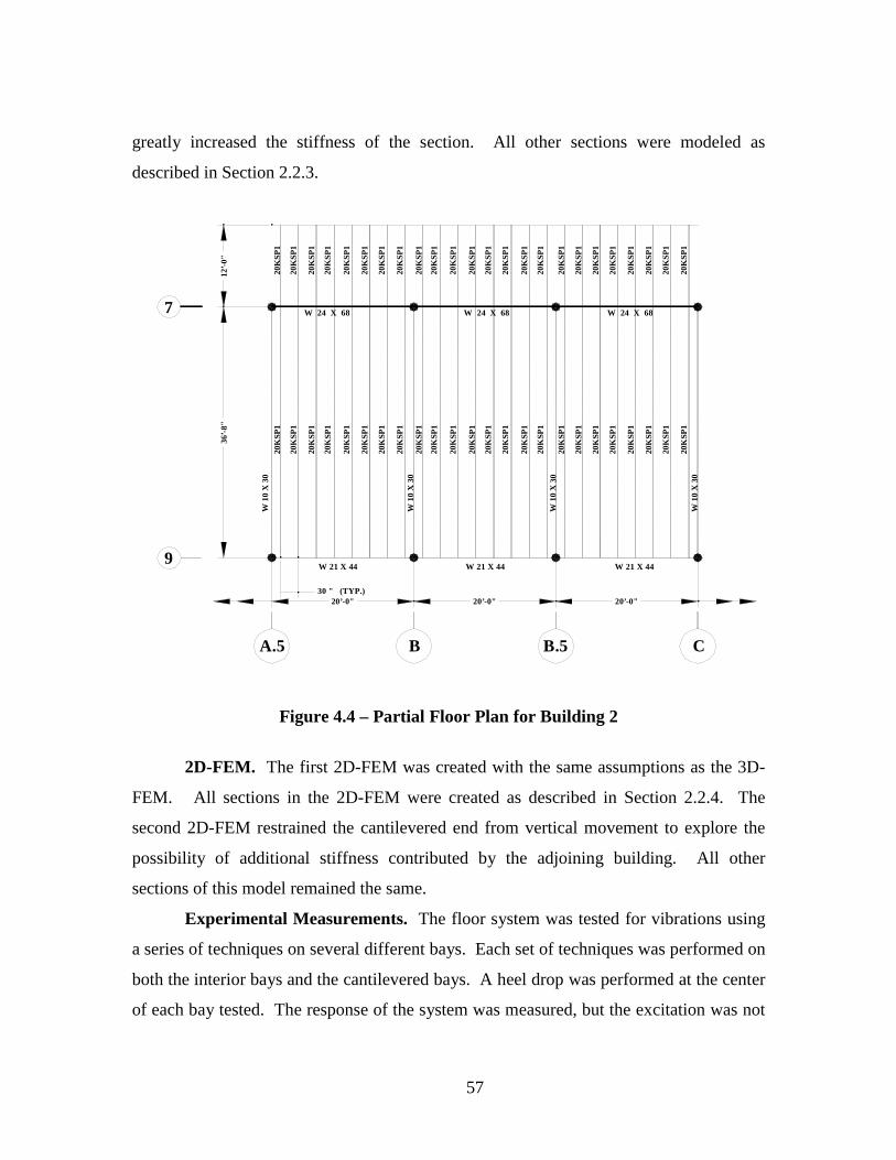
57
greatly increased the stiffness of the section. All other sections were modeled as
described in Section 2.2.3.
20’-0" 20’-0" 20’-0"
36’-
8"12
’-0"
20K
SP1
30 " (TYP.)
20K
SP1
2 0K
SP1
20K
SP1
20K
S P1
20K
SP1
20K
SP1
20K
SP1
20K
SP1
20K
S P1
20K
SP1
20K
S P1
20K
SP1
20K
SP1
2 0K
SP1
20K
SP1
20K
SP1
20K
SP1
20K
SP1
20K
SP1
20K
SP1
20K
SP1
20K
SP1
20K
SP1
2 0K
SP1
20K
SP1
20K
SP1
20K
SP1
20K
SP1
20K
S P1
20K
SP1
20K
SP1
20K
S P1
20K
SP1
20K
SP1
20K
SP1
20K
SP1
2 0K
SP1
20K
SP1
20K
SP1
20K
S P1
20K
SP1
20K
SP1
20K
SP1
20K
SP1
20K
SP1
20K
SP1
20K
SP1
W 1
0 X
30
W 1
0 X
30
W 1
0 X
30
W 1
0 X
30
W 21 X 44W 21 X 44 W 21 X 44
W 24 X 68W 24 X 68 W 24 X 68
A.5 B B.5 C
9
7
Figure 4.4 – Partial Floor Plan for Building 2
2D-FEM. The first 2D-FEM was created with the same assumptions as the 3D-
FEM. All sections in the 2D-FEM were created as described in Section 2.2.4. The
second 2D-FEM restrained the cantilevered end from vertical movement to explore the
possibility of additional stiffness contributed by the adjoining building. All other
sections of this model remained the same.
Experimental Measurements. The floor system was tested for vibrations using
a series of techniques on several different bays. Each set of techniques was performed on
both the interior bays and the cantilevered bays. A heel drop was performed at the center
of each bay tested. The response of the system was measured, but the excitation was not
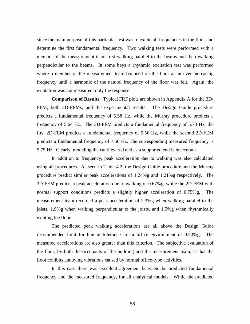
58
since the main purpose of this particular test was to excite all frequencies in the floor and
determine the first fundamental frequency. Two walking tests were performed with a
member of the measurement team first walking parallel to the beams and then walking
perpendicular to the beams. In some bays a rhythmic excitation test was performed
where a member of the measurement team bounced on the floor at an ever-increasing
frequency until a harmonic of the natural frequency of the floor was felt. Again, the
excitation was not measured, only the response.
Comparison of Results. Typical FRF plots are shown in Appendix A for the 3D-
FEM, both 2D-FEMs, and the experimental results. The Design Guide procedure
predicts a fundamental frequency of 5.58 Hz, while the Murray procedure predicts a
frequency of 5.64 Hz. The 3D-FEM predicts a fundamental frequency of 5.73 Hz, the
first 2D-FEM predicts a fundamental frequency of 5.56 Hz, while the second 2D-FEM
predicts a fundamental frequency of 7.56 Hz. The corresponding measured frequency is
5.75 Hz. Clearly, modeling the cantilevered end as a supported end is inaccurate.
In addition to frequency, peak acceleration due to walking was also calculated
using all procedures. As seen in Table 4.2, the Design Guide procedure and the Murray
procedure predict similar peak accelerations of 1.24%g and 1.21%g respectively. The
3D-FEM predicts a peak acceleration due to walking of 0.67%g, while the 2D-FEM with
normal support conditions predicts a slightly higher acceleration of 0.75%g. The
measurement team recorded a peak acceleration of 2.3%g when walking parallel to the
joists, 1.9%g when walking perpendicular to the joists, and 1.5%g when rhythmically
exciting the floor.
The predicted peak walking accelerations are all above the Design Guide
recommended limit for human tolerance in an office environment of 0.50%g. The
measured accelerations are also greater than this criterion. The subjective evaluation of
the floor, by both the occupants of the building and the measurement team, is that the
floor exhibits annoying vibrations caused by normal office-type activities.
In this case there was excellent agreement between the predicted fundamental
frequency and the measured frequency, for all analytical models. While the predicted
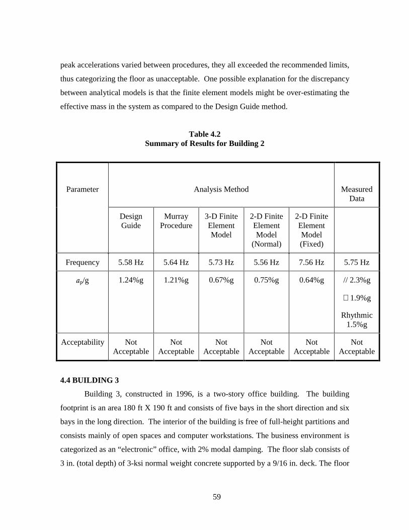
59
peak accelerations varied between procedures, they all exceeded the recommended limits,
thus categorizing the floor as unacceptable. One possible explanation for the discrepancy
between analytical models is that the finite element models might be over-estimating the
effective mass in the system as compared to the Design Guide method.
Table 4.2Summary of Results for Building 2
Analysis Method MeasuredData
Parameter
DesignGuide
MurrayProcedure
3-D FiniteElementModel
2-D FiniteElementModel
(Normal)
2-D FiniteElementModel(Fixed)
Frequency 5.58 Hz 5.64 Hz 5.73 Hz 5.56 Hz 7.56 Hz 5.75 Hz
p/g 1.24%g 1.21%g 0.67%g 0.75%g 0.64%g // 2.3%g
⊥ 1.9%g
Rhythmic1.5%g
Acceptability NotAcceptable
NotAcceptable
NotAcceptable
NotAcceptable
NotAcceptable
NotAcceptable
4.4 BUILDING 3
Building 3, constructed in 1996, is a two-story office building. The building
footprint is an area 180 ft X 190 ft and consists of five bays in the short direction and six
bays in the long direction. The interior of the building is free of full-height partitions and
consists mainly of open spaces and computer workstations. The business environment is
categorized as an “electronic” office, with 2% modal damping. The floor slab consists of
3 in. (total depth) of 3-ksi normal weight concrete supported by a 9/16 in. deck. The floor

60
slab is supported by joists and joist-girders. A detailed framing plan for a typical area of
this building is shown in Figure 4.5. The 24K7 joists (Ieff = 414 in4) are shown in Figure
4.6 and the 24G13N9.0K joist-girders (Ieff = 2195 in4) are shown in Figure 4.7.
24G13N9.0K
31’-8" 31’-8" 31’-8"
36’-
0"36
’-0"
2 3 4 5
A
B
C
D
36’-
0"
24 K
7
24G13N9.0K
24G13N9.0K
24G13N9.0K
Figure 4.5 – Partial Floor Plan for Building 3
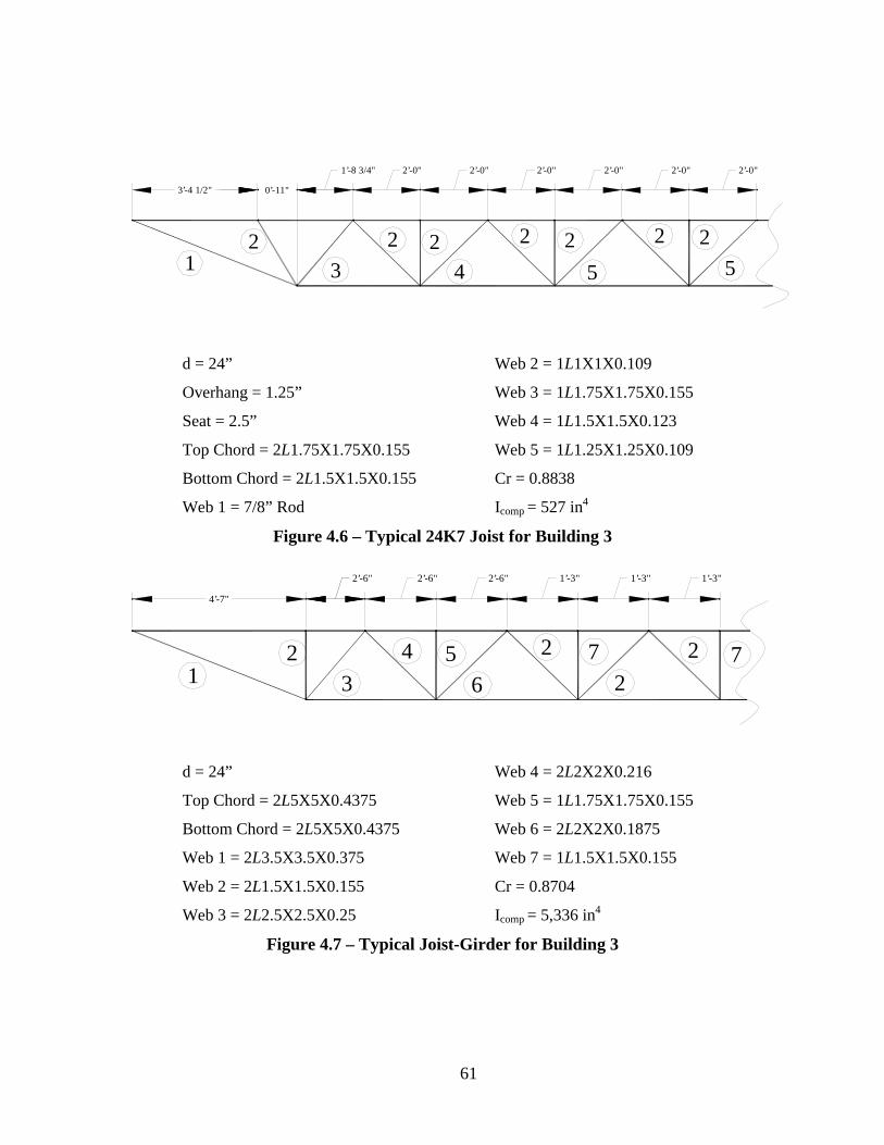
61
3’-4 1/2" 0’-11"
1’-8 3/4" 2’-0" 2’-0" 2’-0" 2’-0"
12
3
2 24
2 2
5
2’-0" 2’-0"
2 2
5
d = 24”
Overhang = 1.25”
Seat = 2.5”
Top Chord = 2L1.75X1.75X0.155
Bottom Chord = 2L1.5X1.5X0.155
Web 1 = 7/8” Rod
Web 2 = 1L1X1X0.109
Web 3 = 1L1.75X1.75X0.155
Web 4 = 1L1.5X1.5X0.123
Web 5 = 1L1.25X1.25X0.109
Cr = 0.8838
Icomp = 527 in4
Figure 4.6 – Typical 24K7 Joist for Building 3
2’-6" 2’-6" 2’-6" 1’-3"
12
3
4 56
2 72
2 7
1’-3" 1’-3"
4’-7"
d = 24”
Top Chord = 2L5X5X0.4375
Bottom Chord = 2L5X5X0.4375
Web 1 = 2L3.5X3.5X0.375
Web 2 = 2L1.5X1.5X0.155
Web 3 = 2L2.5X2.5X0.25
Web 4 = 2L2X2X0.216
Web 5 = 1L1.75X1.75X0.155
Web 6 = 2L2X2X0.1875
Web 7 = 1L1.5X1.5X0.155
Cr = 0.8704
Icomp = 5,336 in4
Figure 4.7 – Typical Joist-Girder for Building 3

62
This floor system was analyzed using the Design Guide procedure, a 3D-FEM,
and a 2D-FEM. The results of these three analyses are compared with experimental test
results.
Design Guide Procedure. The loading on the structure was assumed to include 2
psf of dead load in addition to the weight of the floor slab and supporting members, and 5
psf of live load, since the building was sparsely occupied at the time of testing. The
modal damping in the structure was assumed to be 0.02 because no partitions were
present and the office was categorized as an “electronic” office. A typical interior bay
was analyzed, so the edge conditions for the floor did not affect the results.
The fundamental frequency of the floor was taken to be a function of the
frequency of the joists and the frequency of the joist-girders, related by Dunkerly’s
Equation, given as Equation 1.3. Since the joists are only connected at the top chord, the
50% mass increase allowed for continuity was ignored when calculating the peak
acceleration.
3D-FEM. The 3D-FEM used the same loading assumptions as the Design Guide
procedure. All sections were modeled as described in Section 2.2.3.
2D-FEM. The 2D-FEM was created with the same assumptions as the 3D-FEM.
All sections in the 2D-FEM were created as described in Section 2.2.4.
Experimental Measurements. The floor system was tested for vibrations using
a series of techniques on several different bays. A heel drop was performed at the center
of several bays. The response of the system was measured, but the excitation was not
since the main purpose of this particular test was to excite all frequencies in the floor and
determine the fundamental frequency. Three walking tests were performed with a
member of the measurement team first walking parallel to the joists, then walking
perpendicular to the joists, and finally walking in place taking 48 steps in 15 seconds.
Comparison of Results. Typical FRF plots are shown in Appendix A for the 3D-
FEM, the 2D-FEM, and the experimental results. The Design Guide procedure predicts a
natural frequency of 3.70 Hz, while the 3D-FEM and the 2D-FEM predict natural

63
frequencies of 3.71 Hz and 3.80 Hz respectively. The corresponding measured frequency
is 3.75 Hz.
In addition to frequency, acceleration due to walking was also calculated using
each of the three analytical methods. As seen in Table 4.3, the Design Guide procedure
predicts a peak acceleration due to walking of 1.02%g, which is above the Design Guide
recommended limit for human tolerance in an office environment, while the 3D-FEM and
the 2D-FEM predict essentially the same acceleration due to walking, 0.46%g – 0.49%g,
which is below the limit of 0.50%g. The measurement team recorded a peak acceleration
of 7.7%g when walking parallel to the joists, 6.4%g when walking perpendicular to the
joists, and 27%g when walking in place. The subjective evaluation of the floor, by both
the occupants of the building and the measurement team, is that the floor exhibits
annoying vibrations caused by normal office-type activities.
Table 4.3Summary of Results for Building 3
Analysis Method
Parameter Design Guide 3D FiniteElement Model
2D FiniteElement Model
Measured Data
Frequency 3.70 Hz 3.71 Hz 3.82 Hz 3.75 Hz
p/g 1.11 %g 0.46 %g 0.49 %g // 7.7%g
⊥ 6.4%g
In Place 27%g
Acceptability Not Acceptable Acceptable Acceptable Not Acceptable
In this case there was excellent agreement between the measured fundamental
frequency and the predicted fundamental frequency for all analysis procedures.
However, there was a great discrepancy between the peak acceleration values predicted.

64
While all three methods gave values significantly less than the measured values, only the
Design Guide procedure correctly identified the floor as being unacceptable. One
possible explanation for this is that the finite element models predict a greater effective
mass than the Design Guide does. Mass is inversely proportional to the peak acceleration
response, so a larger mass would lead to a smaller peak acceleration, similar to what
happens in this analysis.
4.5 BUILDING 4
Building 4 was constructed in 1997. The ballroom, where vibrations are a
problem, is an area 180 ft X 220 ft and consists of two bays in the short direction and
eight bays in the long direction. The ballroom is free of columns and partitions. Some
full height partitions are in use below the ballroom in some meeting rooms on the lower
level. The floor slab consists of 5-1/2 in. (total depth) of 4-ksi normal weight concrete
supported by a 3 in. deck. A detailed framing plan for a typical area of this building is
shown in Figure 4.8. The floor slab is supported by hot rolled sections and a series of
built-up plate girders. The effective composite moments of inertia of the beams and
girders are 3050 in4 and 131,000 in4, respectively.
This floor system was analyzed using the Design Guide procedure, and two
different 3D-FEMs. No 2D-FEM was created for this floor. The results of these three
analyses are compared with experimental test results.
Design Guide Procedure. The loading on the structure was assumed to include 8
psf of dead load, in addition to the weight of the floor slab and supporting members, for a
walking analysis and an additional 12.5 psf of live load for a rhythmic analysis. The
modal damping in the structure was assumed to be 0.03 because of the large quantities of
structural steel, flooring, mechanical and electrical equipment present.
An interior portion of the ballroom floor, two bays wide and three bays long, was
analyzed, so the edge conditions for the floor were unimportant. The fundamental
frequency of the floor was taken to be a function of the fundamental frequencies of the
beams and the girders, as related by Equation 1.3. Also, since the slab is supported by

65
hot-rolled beams shear connected to the girders, and the adjacent spans are at least 7/10
of the span in question, the allowed 50% mass increase was included when calculating
the peak acceleration.
BU 60 X 273
W 2
1 X
44
F.5
E.9
876
BU 60 X 273
BU 60 X 273
BU 60 X 273
BU 60 X 273
BU 60 X 273
BU 60 X 273
BU 60 X 273
W 2
1 X
44
W 2
1 X
44
W 2
1 X
44
W 2
1 X
44
W 2
1 X
44
W 2
1 X
44
W 2
1 X
44
W 2
1 X
44
W 2
1 X
44
W 2
1 X
44
W 2
1 X
44
W 2
1 X
44
W 2
1 X
44
W 2
1 X
44
W 2
1 X
44
W 2
1 X
44
W 2
1 X
44
W 2
1 X
44
W 2
1 X
44
W 2
1 X
44
W 2
1 X
44
W 2
1 X
44
W 2
1 X
44
W 2
1 X
44
W 2
1 X
44
W 2
1 X
44
W 2
1 X
44
W 2
1 X
44
W 2
1 X
44
W 2
1 X
44
W 2
1 X
44
W 2
1 X
44
W 2
1 X
44
W 2
1 X
44
W 2
1 X
44
W 2
1 X
44
W 2
1 X
44
W 2
1 X
44
W 2
1 X
44
W 2
1 X
44
W 2
1 X
44
W 2
1 X
44
W 2
1 X
44
W 2
1 X
44
W 2
1 X
44
W 2
1 X
44
W 2
1 X
44
W 2
1 X
44
W 2
1 X
44
W 2
1 X
44
W 2
1 X
44
W 2
1 X
44
W 2
1 X
44
W 2
1 X
44
W 2
1 X
44
W 2
1 X
44
90’-0" 90’-0"
27’-
6"27
’-6"
27’-
6"
Figure 4.8 – Partial Floor Plan for Building 4
3D-FEM. Two 3D-FEMs were created for this analysis. The first model was
created in the same manner as described in Section 2.2.3. The second model was created
with the assumption that each support should be restrained in all three translational
directions. Each model was analyzed both for a walking load and for a dancing load.
The dancing load was applied as a uniform sinusoidal load over one bay of magnitude
12.5 psf and a frequency that is a fraction of the fundamental frequency, but is limited to
the range of one to three hertz.
Experimental Measurements. The floor system was tested for vibrations
differently than other floors in the study. The mass of the floor is so great that a single
individual performing a heel drop is unable to effectively excite the floor. Therefore, two

66
groups of ROTC cadets, one consisting of 26 Cadets and one of 17 Cadets, were asked to
assist in this study. Using an electronic drum, the Cadets marched in time at a variety of
frequencies. Accelerations were recorded for each frequency. A third test was
performed with roughly seventy students actively dancing in order to excite the floor.
Again, accelerations were recorded.
Comparison of Results. Typical FRF plots are shown in Appendix A for both
3D-FEMs, and the experimental results. The Design Guide predicts a fundamental
frequency of 3.82 Hz. The original 3D-FEM predicts a fundamental frequency of 3.67
Hz, while the 3D-FEM with the additional restraints predicts a fundamental frequency of
4.50 Hz. The measured response shows a fundamental frequency of 4.75 Hz. This was
achieved when the Cadets marched at a pacing frequency of 2.4 Hz, or roughly half of the
fundamental frequency of the floor.
In addition to frequency, peak accelerations due to walking and dancing were also
calculated using both analytical methods. As seen in Table 4.4, the Design Guide
procedure predicts a walking acceleration of 0.12%g and a dancing acceleration of
28.6%g. The original 3D-FEM predicts a walking acceleration of 0.1%g, and a dancing
acceleration of 19.6%g. The restrained 3D-FEM predicts a walking acceleration of
0.09%g and a dancing acceleration of 18.7%g. All three walking accelerations are below
the Design Guide recommended limit for human tolerance in an office environment of
0.50%g, but all three accelerations for dancing are above the Design Guide recommended
limit of 2%g for rhythmic activities combined with dining. The measurement team
recorded an acceleration of about 10%g when the Cadets were marching, and an
acceleration of 7%g was recorded under the dancing load. The subjective evaluation of
the floor, by both the occupants of the building and the measurement team, is that the
floor is acceptable under a walking load, but is unacceptable under the conditions it is
likely to be used for, namely, dancing.
In this case, the Design Guide procedure and the original 3D-FEM are in good
agreement with one another in terms of both fundamental frequency and peak walking
acceleration. On the other hand, the restrained 3D-FEM is in good agreement with the

67
measured results in terms of fundamental frequency. Clearly, the column supports are
adding more rigidity to the system than is generally assumed. A strict comparison of the
marching and dancing loads is invalid here, but is useful in order to determine the
acceptability of the floor under the loading that it is likely to see.
Table 4.4Summary of Results for Building 4
Analysis Method
Parameter Design GuideProcedure
3D-FEMOriginal
3D-FEMRestrained
Measured Data
Frequency 3.82 Hz 3.67 Hz 4.50 Hz 4.75 Hz
p/g (Walking) 0.12 %g 0.10 %g 0.09 %g N/A
p/g (Marching) N/A N/A N/A 10 %g
Acceptability Acceptable Acceptable Acceptable Acceptable
p/g (Dancing) 28.6%g 19.6%g 18.7%g 7%g
Acceptability Not Acceptable Not Acceptable Not Acceptable Not Acceptable
4.6 BULDING 5
Building 5, constructed in 1996, is a two-story office. The building footprint is an
area 110 ft X 225 ft and consists of three bays in the short direction and six bays in the
long direction. The building contains numerous demountable partitions and other office
equipment. The building also contains several large openings that affect the vibration
characteristics of the floor. The business environment is categorized as a “paper” office,
with 2.5% modal damping. The floor slab consists of 4 in. (total depth) of 4-ksi normal
weight concrete supported by a 2 in. deck. A detailed framing plan for a typical area of
this building is shown in Figure 4.9. The effective composite moments of inertia of the

68
beams and girders are 1254 in4 and 6256 in4, respectively. This floor system was
analyzed using the Design Guide procedure, a 3D-FEM, and a 2D-FEM. The results of
these three analyses are compared with experimental test results.
W 16 X 26 W 16 X 26W 16 X 26
W 2
4 X
103
W 2
1 X
93
W 2
1 X
101
A
C
D
F
6543
40’-0" 40’-0" 40’-0"
W 16 X 26 W 16 X 26 W 16 X 26
W 16 X 31 W 16 X 31 W 16 X 31
W 16 X 31 W 16 X 31 W 16 X 31
W 16 X 31 W 16 X 31 W 16 X 31
W 16 X 31 W 16 X 31 W 16 X 31
W 16 X 31 W 16 X 31 W 16 X 31
W 16 X 31 W 16 X 31 W 16 X 31
W 14 X 22 W 14 X 22 W 14 X 22
W 14 X 34 W 14 X 34 W 14 X 34
W 16 X 45 W 16 X 45 W 16 X 45
W 16 X 31 W 16 X 45 W 16 X 45
W 14 X 22 W 14 X 34 W 14 X 34
W 2
1 X
93
W 2
1 X
101
W 2
4 X
103
W 2
1 X
93
W 2
1 X
101
W 2
4 X
103
W 2
1 X
93
W 2
1 X
101
W 2
4 X
103
8’-8
"8’
- 2"
9’-6
"9’
-2"
9 ’-0
"9’
-0"
9’-0
"8’
-8"
8’-8
"8’
-10"
6’-4
"8’
-8"
35’-
0"36
’-2"
32’-
6"
Figure 4.9 – Partial Floor Plan for Building 5
Design Guide Procedure. The loading on the structure was assumed to include 8
psf of dead load and no live load, in addition to the weight of the floor slab and
supporting members, since the building was not occupied at the time of testing. The
modal damping in the structure was assumed to be 0.025 because of the presence of
partitions, mechanical equipment, and filing cabinets, hence the categorization of “paper”

69
office. Since the exterior girder was integral with the exterior wall, this member was
assumed to have a very large stiffness. The fundamental frequency of the floor was taken
to be a function of the frequency of the beams and the girders as related by Equation 1.3.
3D-FEM. The 3D-FEM used the same loading assumptions as the Design Guide
procedure. The exterior girder was restrained in the model because the exterior cladding
greatly increased the stiffness of the section. All other sections were modeled as
described in Section 2.2.3.2D-FEM. The 2D-FEM was created with the same
assumptions as the 3D-FEM. All other sections in the 2D-FEM were created as
described in Section 2.2.4.
Experimental Measurements. The floor system was tested for vibrations using
a series of techniques on several different bays. A heel drop was performed at the center
of each bay tested. The response of the system was measured, but the excitation was not
since the main purpose of this particular test was to excite all frequencies in the floor and
determine the first fundamental frequency. Three walking tests were performed with a
member of the measurement team first walking parallel to the beams, then walking
perpendicular to the beams, and finally walking in place, taking 34 steps in 15 seconds.
Comparison of Results. Typical FRF plots are shown in Appendix A for the 3D-
FEM, the 2D-FEM, and the experimental results. The Design Guide procedure predicts a
natural frequency of 3.33 Hz. The 3D-FEM predicts a fundamental frequency of 3.90
Hz, and an even greater response at a frequency of 4.50 Hz. The mode shape, however,
indicates that the smaller frequency is associated with the primary bending mode for this
floor. The 2D-FEM predicts a fundamental frequency of 3.68 Hz. The corresponding
measured frequency is between 3.75 Hz and 4 Hz.
In addition to frequency, acceleration due to walking was also calculated using
each of the three analytical methods. As seen in Table 4.5, there is a large discrepancy
between the values predicted. The Design Guide procedure predicts a peak acceleration
of 0.77%g, while the 3D-FEM predicts a peak walking acceleration of 0.37%g, and the
2D-FEM predicts a peak walking acceleration of 0.85%g. The acceleration predicted by
the Design Guide procedure and the 2D-FEM exceeds the Design Guide recommended

70
limit of 0.50%g for office floors. However, the acceleration predicted by the 3D-FEM
does not. The measurement team recorded an acceleration of 2%g when walking parallel
to the beams, 3%g when walking perpendicular to the beams, and 8.75%g when walking
in place. The subjective evaluation of the floor, by both the occupants of the building and
the measurement team, is that the floor exhibits annoying vibrations caused by normal
office-type activities.
In this case there is relatively good agreement between the predicted and
measured frequencies, with the Design Guide prediction being the furthest away.
However, in terms of peak acceleration, there is very little agreement, except between the
Design Guide procedure and the 2D-FEM. All predictions greatly underestimated the
actual response of the floor, and the 3D-FEM even predicted an acceleration well below
the recommended limit.
Table 4.5Summary of Results for Building 5
Analysis Method
Parameter Design GuideProcedure
3D FiniteElement Model
2D FiniteElement Model
Measured Data
Frequency 3.33 Hz 3.90 Hz 3.68 Hz 3.75 Hz - 4 Hz
p/g 0.77 %g 0.37 %g 0.85 %g // 2%g
⊥ 3%g
In Place 8.75%g
Acceptability Not Acceptable Acceptable Not Acceptable Not Acceptable
4.7 BUILDING 6
Building 6, constructed in 1997, is a three-story office building. The building
footprint occupies an area 56 ft X 112 ft and consists of one bay in the short direction and
five bays in the long direction. At the time of testing, the building was under

71
construction, with only the structural steel and concrete deck in place. The floor slab
consists of 5 in. (total depth) of 4-ksi normal weight concrete supported by a 1-1/2 in.
deck. Both the second and third floors of this building were analyzed. The only
difference between the floors was the size of the joists. For this analysis, the web
members were unavailable, so the effective moment of inertia was calculated based on
the chord sizes and spacing. A detailed framing plan for a typical area of this building is
shown in Figure 4.10.
The floor slab is supported by composite joists resting on hot-rolled sections. The
second floor joists are 40 in. deep with a top chord of 2L2.5X2.5X0.23 and a bottom
chord of 2L3X3X0.30. The third floor joists are 36 in. deep with a top chord of
2L2.5X2.5X0.23 and a bottom chord of 2L3X3X0.25. The effective moments of inertia
for the joists of the second and third floors were 4073 in4 and 2979 in4, respectively.
Both the second and third floors were analyzed using the Design Guide procedure, a 3D-
FEM and a 2D-FEM. The results of these three analyses are compared with experimental
test results.
JOIS
T
D
A
13121110
JOIS
T
JOIS
T
JOIS
T
JOIS
T
JOIS
T
JOIS
T
JOIS
T
JOIS
T
JOIS
T
JOIS
T
JOIS
T
JOIS
T
W 24X84 W 24X84 W 24X84
W 24X84 W 24X84W 24X84
56’-
0"
24’-0" 24’-0" 24’-0"
Figure 4.10 – Partial Floor Plan for Building 6

72
Design Guide Procedure. Since only the structural steel and concrete slab were
in place at the time of testing, no additional loading was assumed. The modal damping in
the structure was assumed to be 0.01 for the same reasons. Since no exterior wall was
present at the time of testing, the edges of the slab were not stiffened. Because of the
spacing of members and the long span of the joists, the frequency of the floor was taken
as the frequency of the joists.
3D-FEM. A 3D-FEM was created for each floor that used the same assumptions
as the Design Guide procedure. Since the web members of the joists were not available,
the effective moment of inertia was calculated based on the chord sizes and spacing. A
frame element with a cross sectional area equal to that of the joists was placed at an
elevation such that the composite moment of inertia of the section was equal to the
effective moment of inertia calculated by hand for the joists. All other sections were
created as described in Section 2.2.3.
2D-FEM. A 2D-FEM was created for each floor using the same assumptions as
the 3D-FEM. All sections were created as described in Section 2.2.4.
Experimental Measurements. The second floor of the building was tested for
vibrations using a heel drop and a walking load. The heel drop was applied at the center
of the floor, while the walking load consisted of a member of the measurement team
walking parallel to the joists at the center of the floor. In each case, the response of the
system was measured, but the excitation was not. The third floor of the building was
tested under a heel drop loading only.
Comparison of Results. Typical FRF plots are shown in Appendix A for the
3D-FEM, 2D-FEM and the experimental results associated with each floor. For the
second floor, the Design Guide procedure predicts a fundamental frequency of 4.47 Hz,
the 3D-FEM predicts a fundamental frequency of 4.40 Hz, while the 2D-FEM predicts a
fundamental frequency of 4.27 Hz. The measurement team recorded a fundamental
frequency of 4.25 Hz. For the third floor, the Design Guide procedure predicts a
fundamental frequency of 3.84 Hz, the 3D-FEM predicts a fundamental frequency of
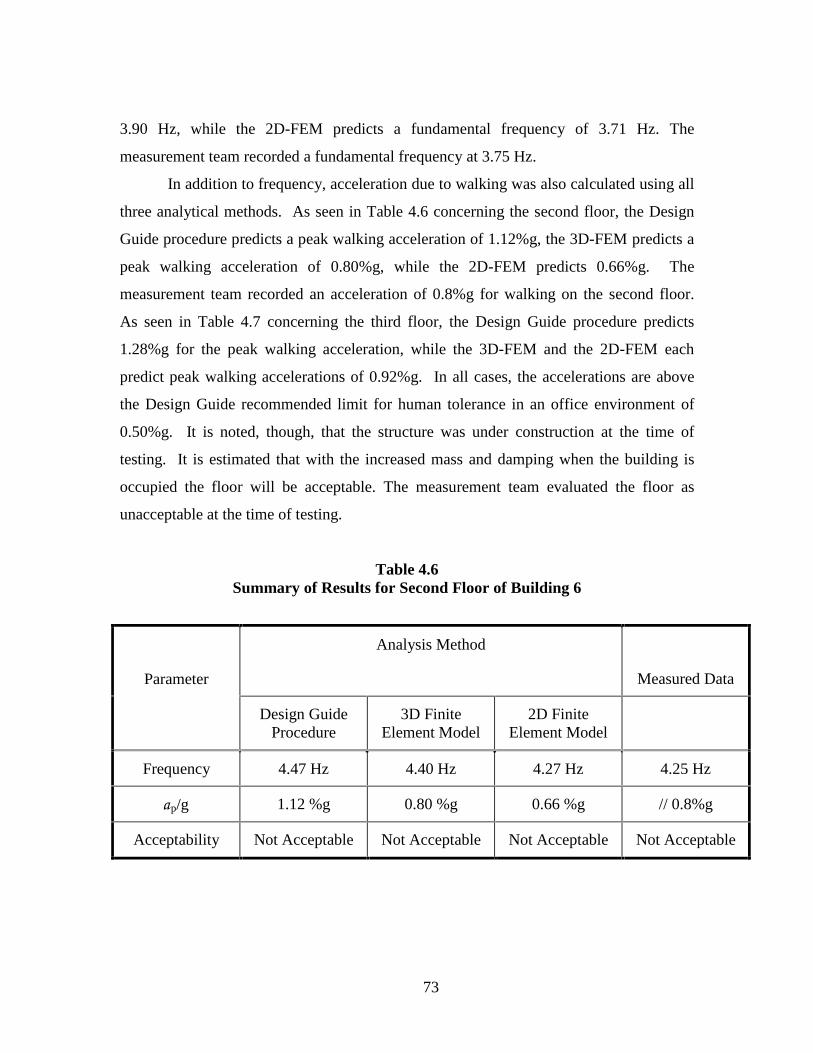
73
3.90 Hz, while the 2D-FEM predicts a fundamental frequency of 3.71 Hz. The
measurement team recorded a fundamental frequency at 3.75 Hz.
In addition to frequency, acceleration due to walking was also calculated using all
three analytical methods. As seen in Table 4.6 concerning the second floor, the Design
Guide procedure predicts a peak walking acceleration of 1.12%g, the 3D-FEM predicts a
peak walking acceleration of 0.80%g, while the 2D-FEM predicts 0.66%g. The
measurement team recorded an acceleration of 0.8%g for walking on the second floor.
As seen in Table 4.7 concerning the third floor, the Design Guide procedure predicts
1.28%g for the peak walking acceleration, while the 3D-FEM and the 2D-FEM each
predict peak walking accelerations of 0.92%g. In all cases, the accelerations are above
the Design Guide recommended limit for human tolerance in an office environment of
0.50%g. It is noted, though, that the structure was under construction at the time of
testing. It is estimated that with the increased mass and damping when the building is
occupied the floor will be acceptable. The measurement team evaluated the floor as
unacceptable at the time of testing.
Table 4.6Summary of Results for Second Floor of Building 6
Analysis Method
Measured DataParameter
Design GuideProcedure
3D FiniteElement Model
2D FiniteElement Model
Frequency 4.47 Hz 4.40 Hz 4.27 Hz 4.25 Hz
p/g 1.12 %g 0.80 %g 0.66 %g // 0.8%g
Acceptability Not Acceptable Not Acceptable Not Acceptable Not Acceptable
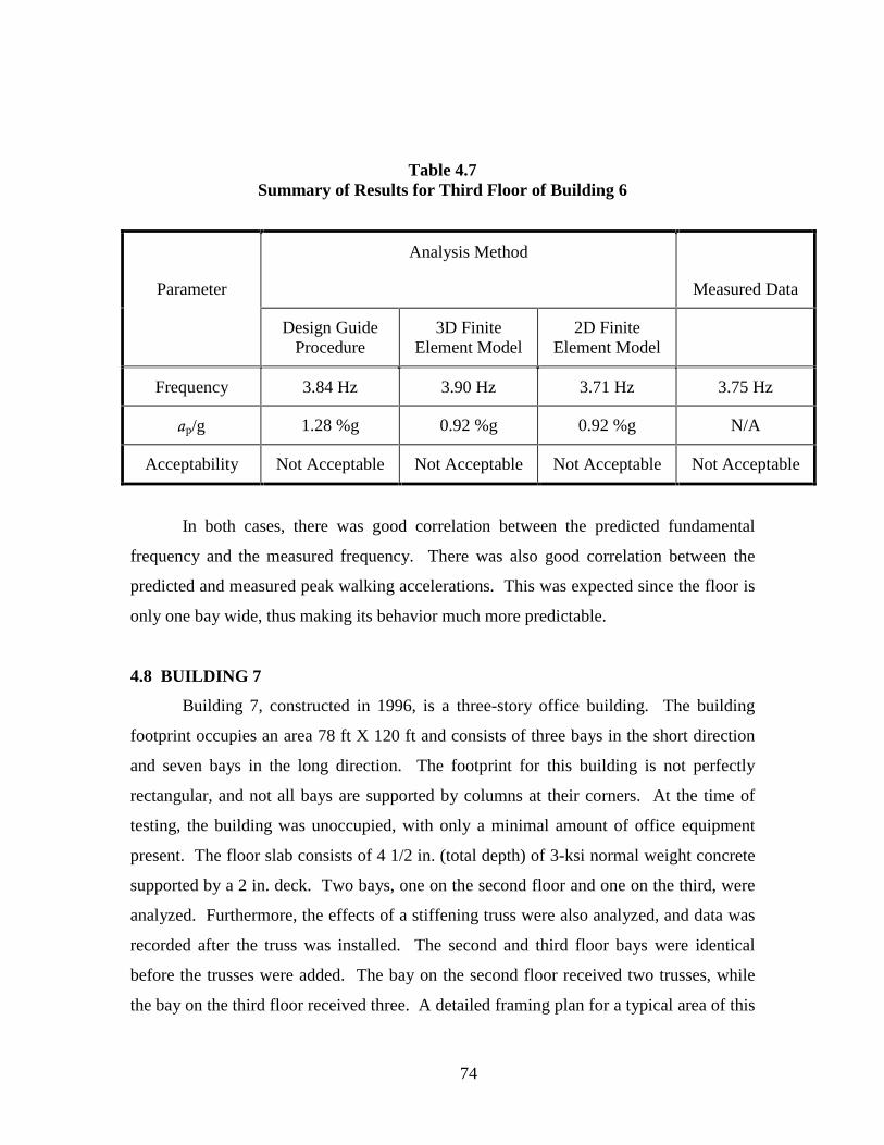
74
Table 4.7Summary of Results for Third Floor of Building 6
Analysis Method
Measured DataParameter
Design GuideProcedure
3D FiniteElement Model
2D FiniteElement Model
Frequency 3.84 Hz 3.90 Hz 3.71 Hz 3.75 Hz
p/g 1.28 %g 0.92 %g 0.92 %g N/A
Acceptability Not Acceptable Not Acceptable Not Acceptable Not Acceptable
In both cases, there was good correlation between the predicted fundamental
frequency and the measured frequency. There was also good correlation between the
predicted and measured peak walking accelerations. This was expected since the floor is
only one bay wide, thus making its behavior much more predictable.
4.8 BUILDING 7
Building 7, constructed in 1996, is a three-story office building. The building
footprint occupies an area 78 ft X 120 ft and consists of three bays in the short direction
and seven bays in the long direction. The footprint for this building is not perfectly
rectangular, and not all bays are supported by columns at their corners. At the time of
testing, the building was unoccupied, with only a minimal amount of office equipment
present. The floor slab consists of 4 1/2 in. (total depth) of 3-ksi normal weight concrete
supported by a 2 in. deck. Two bays, one on the second floor and one on the third, were
analyzed. Furthermore, the effects of a stiffening truss were also analyzed, and data was
recorded after the truss was installed. The second and third floor bays were identical
before the trusses were added. The bay on the second floor received two trusses, while
the bay on the third floor received three. A detailed framing plan for a typical area of this

75
building is shown in Figure 4.11. The area studied, framed by column lines 1 and 5 and
column lines E and F, is shaded. The effective composite moments of inertia for the
W12X19 beams, and the W14X22 girders were 559 in4 and 798 in4, respectively.
W 14 X 22W 16 X 31
W 8 X 10
W 12 X 19 W 14 X 22 W 18 X 40
W 16 X 26W 12 X 19
W 12 X 19W 21 X 44
W 14 X 22
W 8 X 10
W 8
X 1
0W
8 X
10
W 8
X 1
0
W 8
X 1
0W
8 X
10
W 1
0 X
12
W 8
X 1
0W
8 X
10
W 1
0 X
12
W 1
2 X
19
W 8
X 1
0W
10
X 1
2
W 1
2 X
19
W 8
X 1
0W
10
X 1
2
W 1
2 X
19
W 8
X 1
0W
10
X 1
2
W 1
2 X
19
W 8
X 1
0W
10
X 1
2
W 1
2 X
19
W 8
X 1
0W
10
X 1
2
W 1
2 X
19
W 8
X 1
0W
10
X 1
2
W 1
2 X
19
W 8
X 1
0W
10
X 1
2
W 1
2 X
19
W 8
X 1
0W
10
X 1
2
W 8
X 1
0W
8 X
10
W 8
X 1
0
W 8
X 1
0W
8 X
10
W 8
X 1
0
A E F G H
6
5
3
8
1
14’-4" 29’-8" 24’-9"
10’-0"
22’-
10"
18’-
4"31
’-10
"
16’-
10"
W 8 X 10
Figure 4.11 – Partial Floor Plan for Building 7
The floor slab is supported entirely by hot-rolled sections. The stiffening truss
that was added after initial measurements were taken is shown in Figure 4.12. In all
cases, the trusses were added to the middle 10 ft of the section that was stiffened. On the

76
second floor, trusses were added to the W12X19 along column line E and to the W12X19
located 14 ft – 9 in. to the right, yielding an effective composite moment of inertia of
1394 in4. On the third floor, trusses were added at the same location as the floor below as
well as the W14X22 girder along column line 5, yielding an effective composite moment
of inertia of 1739 in4. Both the second and third floors were analyzed using the Design
Guide procedure, and a 3D-FEM for the initial case and for the case with the additional
trusses. The results of these analyses are compared with experimental test results.
1’-8"
Bottom Flange ofHot-Rolled Section
WT4X51 ∠ 1 1/8" X 1 1/8" X 1/8"
1’ - 8"1’ - 8"
6’ - 8"
Figure 4.12 – Stiffening Truss for Building 7
Design Guide Procedure. The loading on the structure was assumed to include
the self weight of the structure and an additional 2 psf of dead load because there was
minimal equipment located on the floor at the time of testing. The modal damping in the
structure was assumed to be 0.03 because of the ceiling and mechanical equipment
present. Since the edge of the floor slab was integral with the exterior wall, the exterior
girder was stiffened. The fundamental frequency of the bay was taken to be a function of
the fundamental frequency of the beams and the girders. For the cases where a stiffening
truss was added, the fundamental frequency of the bay was taken to be a function of the
fundamental frequency of the stiffened beams and the girder.
3D-FEM. Three 3D-FEMs were created for this building which used the same
loading and damping assumptions as the Design Guide procedure. The first 3D-FEM

77
modeled both the second and third floors before the trusses were added. The other two
3D-FEMs modeled the effect of the stiffening trusses by including the actual members
used. All sections were created as described in Section 2.2.3.
Experimental Measurements. Both floors of the building were tested in the
same manner, both before and after the trusses were added. For each case, a heel drop
and two walking loads were used. The heel drop was applied at the center of the bay,
while the walking loads consisted of a member of the measurement team first walking
parallel to the beams at the center of the bay, and then walking perpendicular to the
beams. In all cases, the response of the system was measured, but the excitation was not.
Comparison of Results. Typical FRF plots are shown in Appendix A for all 3D-
FEM analyses and all experimental results. The FRF from the second floor 3D-FEM
without the trusses is shown first, followed by the experimental FRF for the same case.
Then the FRF from the second floor 3D-FEM with the trusses is shown, followed by the
experimental FRF. Results for the third floor follow the same pattern. The Design Guide
procedure predicts a fundamental frequency of 4.18 Hz, while the 3D-FEM predicts a
fundamental frequency of 5.57 Hz before the trusses were added. The corresponding
measured frequency is 5.75 Hz for the second floor and 5.50 Hz for the third. The
Design Guide procedure predicts a fundamental frequency of 5.16 Hz for the second floor
after the trusses were added. The 3D-FEM for the same area predicts a fundamental
frequency of 5.71 Hz., while the measured frequency is 6.25 Hz. The Design Guide
procedure predicts a fundamental frequency of 6.17 Hz for the third floor after the trusses
were added. The 3D-FEM for the same area predicts a fundamental frequency of 5.83
Hz., while the measured frequency is 6.5 Hz.
In addition to frequency, acceleration due to walking was also calculated using
both analytical methods. As seen in Tables 4.8 and 4.9, the Design Guide procedure
predicts a peak acceleration due to walking of 0.95%g before the trusses were added,
while the 3D-FEM predicts a peak acceleration of 1.50%g. After the trusses were added
on the second floor, the Design Guide procedure predicts a peak acceleration of 0.70%g,
while the 3D-FEM predicts 1.27%g. For the third floor, the Design Guide predicts

78
0.52%g as compared to 1.10%g for the 3D-FEM. The measurement team recorded a
number of peak accelerations due to walking on the floor both before and after the trusses
were installed. In all cases, both the predicted values of peak acceleration and the
measured response of the system are above the Design Guide limit of 0.50%g for an
office environment. The subjective evaluation of the occupants of the building and the
measurement team is that both bays exhibited annoying levels of vibration before the
trusses were added, but do not exhibit annoying levels of vibration now that the trusses
are in place.
Before the trusses were added, the Design Guide procedure did not accurately
predict the fundamental frequency of the bays, while the 3D-FEM predicted values that
closely matched the experimental results. Neither model accurately predicted the peak
accelerations. After the trusses were added, both models predicted higher fundamental
frequencies and lower peak accelerations, as expected. However, none of the predicted
values were comparable to the measured values with the exception of the third floor
where the Design Guide predicted a fundamental frequency that was close to the
measured frequency. The irregular column spacing and complex framing scheme for this
floor made accurate predictions exceedingly difficult to make.
Table 4.8Summary of Results for Second Floor of Building 7
Analysis Method
Parameter DesignGuide
Procedure
No Truss
3D-FEM
No Truss
DesignGuide
Procedure
With Truss
3D-FEM
With Truss
MeasuredData
No Truss
MeasuredData
With Truss
Frequency 4.18 Hz 5.57 Hz 5.16 Hz 5.71 Hz 5.75 Hz 6.25 Hz
p/g 0.95%g 1.50%g 0.70 %g 1.27%g // 3.6%g
⊥ 2.1%g
// 2.2%g
⊥ 0.5%g
Acceptability NotAcceptable
NotAcceptable
NotAcceptable
NotAcceptable
NotAcceptable
Acceptable

79
Table 4.9Summary of Results for Third Floor of Building 7
Analysis Method
Parameter DesignGuide
Procedure
No Truss
3D-FEM
No Truss
DesignGuide
Procedure
With Truss
3D-FEM
With Truss
MeasuredData
No Truss
MeasuredData
With Truss
Frequency 4.18 Hz 5.57 Hz 6.17 Hz 5.83 Hz 5.5 Hz 6.50 Hz
p/g 0.95%g 1.50%g 0.52 %g 1.10%g // 2.5%g
⊥ 2.7%g
// 1.9%g
⊥ 1.4%g
Acceptability NotAcceptable
NotAcceptable
NotAcceptable
NotAcceptable
NotAcceptable
Acceptable
4.9 BUILDING 8
Building 8, constructed in 1999, is a four-story academic building. The building
has several wings and a non-rectangular footprint. In general, the building is three bays
wide and more than five bays long. The exterior bays are designed as classrooms, while
the interior bay consists of two cantilevered hallways and a number of large openings. It
is assumed, therefore, that each side of the building will vibrate independently, and so
only half of the entire floor will be modeled. At the time of testing, the building was
open to the air, with only the structural steel and concrete deck in place. The floor slab
consists of 6 in. (total depth) of 4-ksi normal weight concrete supported by a 3 in. deck.
Two different areas of the second floor were analyzed. A detailed framing plan for the
first area tested is shown in Figure 4.13, while the second area is shown in Figure 4.14.
The floor slab is supported by a combination of composite joists and hot-rolled
sections resting on hot-rolled girders. The joists in the first area are 26 in. deep with a top
and bottom chord of 2L4X4X0.44. The joist seats are 5 in. and the joists are cantilevered

80
over the W27 girders, with the bottom chord attached to the girder. The effective
moment of inertia for the composite joist is 3852 in4.
W 10 X 22
W 2
7 X
94
C 6 X 12
G
J
987640
’-6"
7’-1
"
30’-0" 30’-0" 30’-0"JO
IST
W 2
4 X
55
JOIS
T
JOIS
T
W 2
7 X
94
J OIS
T
JOIS
T
W 2
4 X
55
JOIS
T
C 6 X 12C 6 X 12
W 27 X 114 W 27 X 114 W 27 X 114
BLOCK WALL BLOCK WALL BLOCK WALL
W 10 X 22W 10 X 22W 10 X 22
Figure 4.13 – Area 1 for Building 8
The joists for the second area are the same as the joists for the first area with the
exception of their length. The effective moment of inertia for the composite joist is 3586
in4.
Both areas were analyzed using the Design Guide procedure, a 3D-FEM and a
2D-FEM. The results of these three analyses are compared with experimental test results.
Design Guide Procedure. The loading on the structure was assumed to be zero,
since only the structural steel and concrete slab were in place at the time of testing. The
modal damping in the structure was assumed to be 0.01 for the same reasons. Since no
exterior wall was present at the time of testing, the edges of the slab were not stiffened.
3D-FEM. A 3D-FEM was created for each area, which used the same
assumptions as the Design Guide procedure. Since the web members of the joists were
not available, the effective moment of inertia was calculated based on the chord sizes and
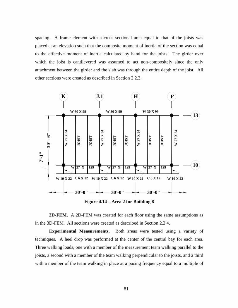
81
spacing. A frame element with a cross sectional area equal to that of the joists was
placed at an elevation such that the composite moment of inertia of the section was equal
to the effective moment of inertia calculated by hand for the joists. The girder over
which the joist is cantilevered was assumed to act non-compositely since the only
attachment between the girder and the slab was through the entire depth of the joist. All
other sections were created as described in Section 2.2.3.
W 10 X 22W
27
X 8
4C 6 X 12
10
13
FHJ.1K
30’ -
6"
7’-1
"
30’-0" 30’-0" 30’-0"
JOIS
T
W 2
7 X
84
JOIS
T
JOIS
T
W 2
7 X
84
J OIS
T
JOIS
T
W 2
7 X
84
JOIS
T
C 6 X 12C 6 X 12
W 27 X 129 W 27 X 129 W 27 X 129
W 30 X 99 W 30 X 99 W 30 X 99
W 10 X 22W 10 X 22W 10 X 22
Figure 4.14 – Area 2 for Building 8
2D-FEM. A 2D-FEM was created for each floor using the same assumptions as
in the 3D-FEM. All sections were created as described in Section 2.2.4.
Experimental Measurements. Both areas were tested using a variety of
techniques. A heel drop was performed at the center of the central bay for each area.
Three walking loads, one with a member of the measurement team walking parallel to the
joists, a second with a member of the team walking perpendicular to the joists, and a third
with a member of the team walking in place at a pacing frequency equal to a multiple of
82
the fundamental frequency of the floor, were recorded. Additionally, rhythmic excitation
was applied at the center of the central bay in each area. In all cases, the response of the
system was measured, but the excitation was not.
Comparison of Results. Typical FRF plots are shown in Appendix A for the 3D-
FEM, 2D-FEM and the experimental results associated with each area. For the first area,
the Design Guide procedure predicts a fundamental frequency of 7.41 Hz, the 3D-FEM
predicts a fundamental frequency of 8.59 Hz, while the 2D-FEM predicts a fundamental
frequency of 8.63 Hz. The measurement team recorded a fundamental frequency of 9.0
Hz. For the second area, the Design Guide procedure predicts a fundamental frequency
of 6.12 Hz, 3D-FEM predicts a fundamental frequency of 6.04 Hz, while the 2D-FEM
predicts a fundamental frequency of 6.14 Hz. The measurement team recorded a
fundamental frequency of 6.75 Hz.
In addition to frequency, acceleration due to walking was also calculated using all
three analytical methods. As seen in Table 4.10 for the first area, the Design Guide
procedure predicts a peak acceleration due to walking of 0.97%g, the 3D-FEM predicts
0.75%g, while the 2D-FEM predicts 0.88%g. The measurement team recorded a peak
walking acceleration of 1.0%g when walking parallel to the joists and 0.9%g when
walking perpendicular to the joists in the first area. When stepping 42 times in 15
seconds, the team recorded a peak acceleration of 10.5%g. When the first area was
rhythmically excited, a peak acceleration of 2.5%g was recorded.
As seen in Table 4.11 for the second area, the Design Guide procedure predicts a
peak acceleration due to walking of 0.89%g, while the 3D-FEM predicts 0.41%g and the
2D-FEM predicts 1.28%g. The measurement team recorded a peak walking acceleration
of 1.1%g when walking parallel to the joists, and 0.7%g when walking perpendicular to
the joists. When stepping 45 times in 15 seconds, the team recorded a peak acceleration
of 6.3%g. When the second area was rhythmically excited, the measured acceleration
peaked at 1.2%. The team evaluated the floor as unacceptable at the time of
measurement.

83
Table 4.10Summary of Results for Area One of Building 8
Analysis Method
Parameter Design Guide 3D FiniteElement Model
2D FiniteElement Model
Measured Data
Frequency 7.41 Hz 8.59 Hz 8.63 Hz 9.0 Hz
p/g 0.97 %g 0.75 %g 0.88 %g // 1.0%g
⊥ 0.9%g
Rhythmic 2.5%g
Acceptability Not Acceptable Not Acceptable Not Acceptable Not Acceptable
Table 4.11Summary of Results for Area Two of Building 8
Analysis Method
Parameter Design Guide 3D FiniteElement Model
2D FiniteElement Model
Measured Data
Frequency 6.12 Hz 6.04 Hz 6.14 Hz 6.75 Hz
p/g 0.89 %g 0.41 %g 1.28 %g // 1.1%g
⊥ 0.7%g
Rhythmic 1.2%g
Acceptability Not Acceptable Not Acceptable Not Acceptable Not Acceptable
In all cases but the 3D-FEM for the second area, the accelerations are above the
Design Guide recommended limit for human tolerance in an office environment of
84
0.50%g,. It is noted, though, that the structure was still under construction at the time of
testing. It is estimated that with the increased mass and damping when the building is
occupied the floor will be acceptable.
For the first area, there was good correlation between both the predicted
frequencies and accelerations and the measured frequencies and accelerations, with the
exception of the Design Guide procedure which significantly underestimated the
fundamental frequency of the floor. For the second area, the predicted frequencies were a
bit lower than the frequency measured, and the peak walking accelerations were widely
dispersed. The 3D-FEM predicted a much lower acceleration than was measured or
predicted by the other analyses, while the 2D-FEM predicted an acceleration that was
higher than either the measured or predicted values from other analyses.
4.10 BUILDING 9
Building 9, constructed in 1998, is an auditorium. The area of concern in this
building is a balcony that is supported by a plate girder spanning 99 ft. The balcony is
sloped, and each row of seats rests one step higher than the row in front, on its own
concrete pad. A plan view of the structural steel framing is shown in Figure 4.15. The
elevations for the endpoints of members are shown in parentheses, taking the centroid of
the plate girder as elevation zero.
The W10X22’s, Figure 4.16, are stiffened from the free end to a point 5 ft 1½ in.
on the opposite side of the plate girder by a kicker. Since the slab is not continuous over
the steel, it is assumed to have no effect on the stiffness of the floor, but the mass of the
concrete is included in the analysis. The plate girder consists of two 16 in. by 2 in.
flanges connected by a 44 in. by 3/8 in. web. The calculated moment of inertia for this
section is approximately 36,500 in4.
FEM Analysis. This structure was analyzed differently than other floors in this
study. A 3D-FEM was the only analysis performed. The concrete slab was not included
in the model for stiffness, but the mass of the concrete was included. In addition, it was
assumed that 40 psf of dead load, which includes the concrete, and 25 psf of live load

85
were present at the time the floor was analyzed. The modal damping for this floor was
not estimated since the acceleration of the floor was not required. Only the fundamental
frequency of the floor and some suggested remedies for the vibration problem were
explored.
W 10 X 100
W 16 X 67
W 14 X 30
W 10 X 22
Plate G irder
Fixed SupportFixed Support
(-14’-4")
(0’-0")
(3’-6")
(-1’-9")
35’ - 5"
9’ - 2"
54’ - 5"
14’-0"
29’ - 5"
4’ - 0"
4 @ 8’ - 0"
Figure 4.15 – Steel Framing Plan for Building 9
The structural steel members in this frame were created as described in Section
2.2.3, with one exception. Instead of using the unit weight and unit mass of steel for each
member, a unit weight and unit mass were calculated separately for each section based on
the tributary loading of that section.
In addition to the as-built analysis described above, several proposed remedies for
the control of the vibrations induced by a lively crowd were also analyzed. The first
solution included the addition of two columns at 8 ft 0 in. from the support along the
W10X100s and the addition of two more columns at 13 ft 6 in. from either end of the
plate girder. The second solution was identical to the first except that the columns along
the plate girder were moved to 21 ft 5 ½ in. from the end of the plate girder. The third

86
proposed remedy consisted of two 16 in. by 2 in. plates welded to the bottom flange of
the plate girder separated by an 18 in. by 3/8 in. vertical plate.
5’-1 1/2"4’-10 1/2"
2’-6"
1’-0"
C8X11.8
1
1
1
0.31
Plate Girder
CL W10X22
Kicker
Figure 4.16 – Kicker For Building 9
Results. The results of the various analyses for this building are shown in Table
4.12. The frequency predicted by the 3D-FEM for the as-built case was 2.65 Hz. The
frequency of the system under the given loading is actually 2.7 Hz. This frequency was
estimated from an incident that occurred shortly after the building was opened. Audience
members attending a rock concert bounced in rhythm with a song being played and
caused disturbing vibrations in the balcony by driving it to resonance. The frequency of
the song is known to be 2.7 Hz; therefore, the frequency of the system under the loading
present at the time of the concert was estimated to also be 2.7 Hz.
The first retrofit solution proposed increased the predicted frequency of the
system to 5.40 Hz. The second proposed retrofit solution increased the predicted
frequency to 6.60 Hz. The third proposed retrofit solution only increased the frequency

87
to 2.95 Hz. None of the proposed retrofit solutions have been completed as of yet, so no
new test data is available for comparison.
Table 4.12Summary of Results for Building 9
Finite Element Models MeasuredData
Parameter 3D-FEM
As Built
3D-FEM
Retrofit #1
3D-FEM
Retrofit #2
3D-FEM
Retrofit #3
Frequency 2.65 Hz 5.40 Hz 6.60 Hz 2.95 Hz 2.7 Hz
4.11 LABORATORY FLOOR 1
Laboratory Floor 1, constructed in 1998, is a single bay, joist-supported floor.
The floor is approximately 31 ft X 31 ft, and the floor slab consists of 3 in. (total depth)
of 3.9-ksi normal weight concrete supported by a 0.6 in. deck. A detailed framing plan
for the floor is shown Figure 4.17.
This floor system was analyzed using the Design Guide procedure, two 2D-
FEMs, and one 3D-FEM. Two analyses were needed to account for some discrepancy in
the effective moment of inertia of the joists. The calculated moment of inertia for the
joists and the measured moment of inertia for the joists were different. Therefore, two
sets of analyses were run. The theoretical moment of inertia of the bare joist is 1074 in4,
but the measured moment of inertia is only 860 in4. The joist used is shown in Figure
4.18. The results of all analyses are compared with experimental test results.
Design Guide Procedure. The additional loading on the structure was assumed
to be zero, since the floor was bare at the time of testing. The modal damping in the
structure was assumed to be 0.01 for the same reason. The joists rest on a concrete
masonry wall, so the fundamental frequency of the floor was taken to be the fundamental
frequency of the joists. Since the edges of the floor are free, the structure was assumed to

88
behave as a mezzanine. One analysis was performed using the predicted moment of
inertia of the bare joist, which yielded an effective moment of inertia of 1546 in4. A
second analysis was performed using the measured moment of inertia of the bare joist,
which yielded an effective moment of inertia of 1314 in4.
30’-9"
31’-4"
13 @ 2’-2 7/8"
14 36LH 1500-T1
Figure 4.17 – Floor Plan for Laboratory Floor 1

89
3’-3" 1’-11"
0’-2 1/2" 2’-6" 2’-6" 2’-6" 2’-6"
12
3
4 65
6 6
7
d = 36”
Top Chord = 2L3X3X0.25
Bottom Chord = 2L2.5X2.5X0.212
Web 1 = 2L2X2X0.232
Web 2 = 1L1.5X1.5X0.151
Web 3 = 2L2.5X2.5X0.151
Web 4 = 2L1.25X1.25X0.13
Web 5 = 1L2X2X0.187
Web 6 = 1L1.25X1.25X0.13
Web 7 = 1L1.75X1.75X0.155
Cr = 0.7582
Ichords – theory = 1074 in4
Ichords – measured = 860 in4
Figure 4.18– Typical Joist for Laboratory Floor 1
3D-FEM. The 3D-FEM used the same loading assumptions as the Design Guide
procedure. The ends of the joists were simply supported to model the fact that the
masonry wall will not have any effect on the vibration characteristics of the floor. The
predicted moment of inertia for the joist matched the measured moment of inertia in the
3D-FEM. All other sections were modeled as described in Section 2.2.3.
2D-FEM. Two 2D-FEMs were created with the same assumptions as the Design
Guide procedure. All other sections in the 2D-FEM were created as described in Section
2.2.4.
Experimental Measurements. The floor system was tested for vibrations using
a series of techniques. A heel drop was performed at the center of the floor. The
response of the system was measured, but the excitation was not since the main purpose
of this particular test was to excite all frequencies in the floor and determine the first
fundamental frequency. Three walking tests were performed with a member of the

90
measurement team first walking parallel to the joists, secondly walking perpendicular to
the joists, and finally walking in place at a pace that was a harmonic of the fundamental
frequency of the floor, 43 steps in 15 seconds.
Comparison of Results. Typical FRF plots are shown in Appendix A for the 3D-
FEM, both 2D-FEMs, and the experimental results. The Design Guide procedure
predicts a fundamental frequency of 17.6 Hz for the theoretical moment of inertia and
16.2 Hz for the measured moment of inertia. The 3D-FEM predicts a fundamental
frequency of 16.92 Hz. The 2D-FEM corresponding to the theoretical moment of inertia
of the joists shows a fundamental frequency of 18 Hz, while the 2D-FEM corresponding
to the measured moment of inertia of the joists shows a fundamental frequency of 16.58
Hz. The corresponding measured frequency is 16.75 Hz.
In addition to frequency, acceleration due to walking was calculated using each of
the analytical methods. As seen in Table 4.13, the Design Guide procedure predicts a
peak walking acceleration of 0.12%g for the theoretical case and 0.19%g for the
measured case. The 3D-FEM predicts a peak walking acceleration of 0.06%g. The 2D-
FEM predicts a peak walking acceleration of 0.06%g for the theoretical case and 0.1%g
for the measured case. The measurement team record peak walking accelerations equal to
0.044%g, 0.05%g, and 0.23%g for walking perpendicular to the joists, walking parallel to
the joists, and walking in place, respectively. The predicted walking accelerations are all
below the Design Guide recommended limit for human tolerance in an office
environment of 0.5%g. The measured accelerations are also below this same limit. The
subjective evaluation of the floor, by the measurement team, is that the floor does not
exhibit annoying vibrations caused by walking even in the bare state.
In this case, the predicted fundamental frequencies closely matched the measured
value. This is of particular note since the 3D-FEM correctly predicted the moment of
inertia of the joists based on the actual member properties. The calculations for the
moment of inertia of the joist yielded results that were quite different from the measured
results which required that two analyses be run for both the Design Guide procedure and
the 2D-FEM, for comparison. In terms of walking acceleration, the Design Guide

91
procedure overestimated the response, while the 3D-FEM and the 2D-FEM for the
measured case closely matched the measured response.
Table 4.13Summary of Results for Laboratory Floor 1
Analysis Method
Parameter Design Guide Procedure 3D-FEM 2D-FEM MeasuredData
TheoreticalMoment of
Inertia
MeasuredMoment of
Inertia
TheoreticalMoment of
Inertia
MeasuredMoment of
Inertia
Frequency 17.60Hz 16.22 Hz 16.92 Hz 18.00 Hz 16.58 Hz 16.75 Hz
p/g 0.12 %g 0.19%g 0.06%g 0.06%g 0.10%g ⊥ 0.044%g
// 0.05%g
In Place0.23%g
Acceptability Acceptable Acceptable Acceptable Acceptable Acceptable Acceptable
4.12 LABORATORY FLOOR 2
Laboratory Floor 2, constructed in 1996, is a single bay, joist-supported floor.
The floor is approximately 31 ft X 32 ft, and the floor slab consists of 2-1/2 in. (total
depth) of 4.2-ksi light weight concrete supported by a 1 in. deck. A detailed framing
plan for the floor is shown in Figure 4.19.
This floor system was analyzed using the Design Guide procedure, a 2D-FEM,
and a 3D-FEM. A typical joist used for this floor is shown in Figure 4.20, with the web
members following. A typical joist-girder is shown in Figure 4.21, with the web
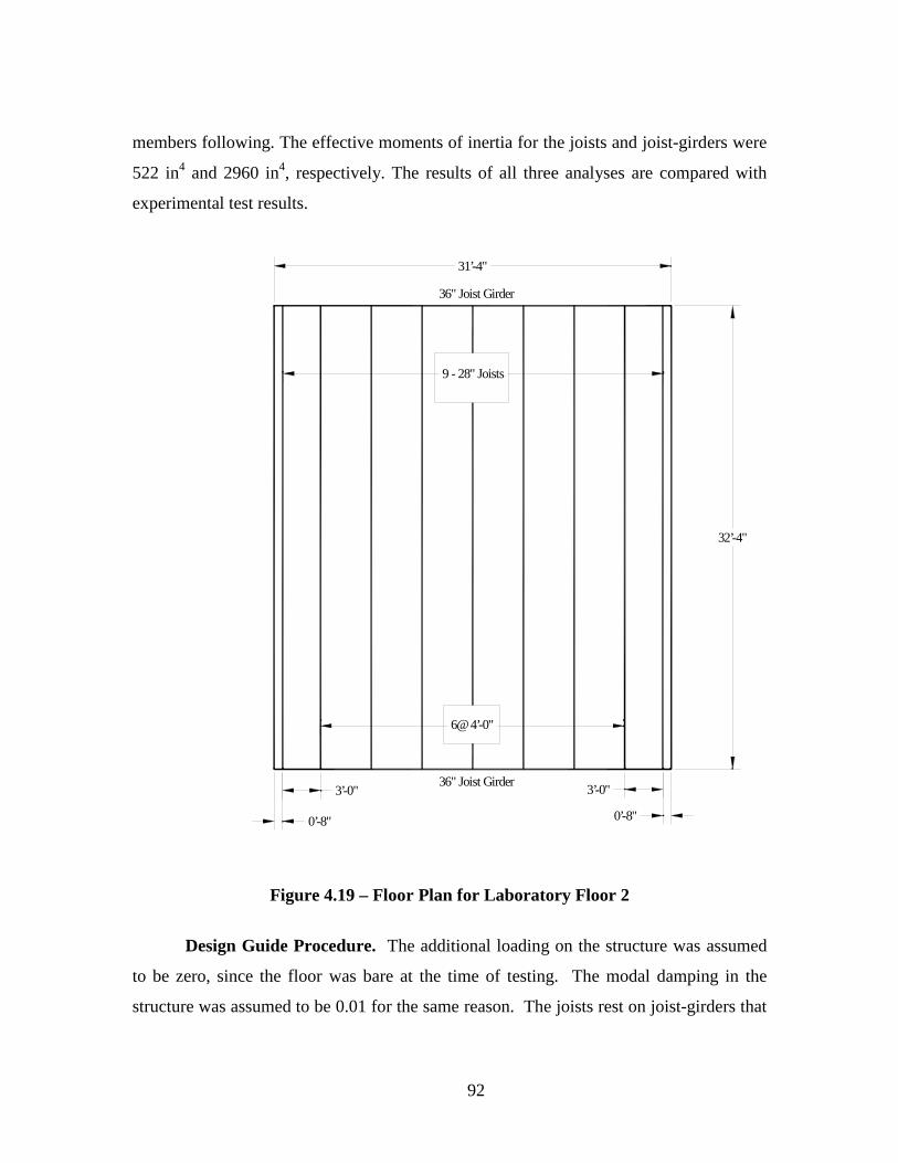
92
members following. The effective moments of inertia for the joists and joist-girders were
522 in4 and 2960 in4, respectively. The results of all three analyses are compared with
experimental test results.
32’-4"
31’-4"
0’-8"
3’-0"
6@ 4’-0"
0’-8"
3’-0"
9 - 28" Joists
36" Joist Girder
36" Joist Girder
Figure 4.19 – Floor Plan for Laboratory Floor 2
Design Guide Procedure. The additional loading on the structure was assumed
to be zero, since the floor was bare at the time of testing. The modal damping in the
structure was assumed to be 0.01 for the same reason. The joists rest on joist-girders that
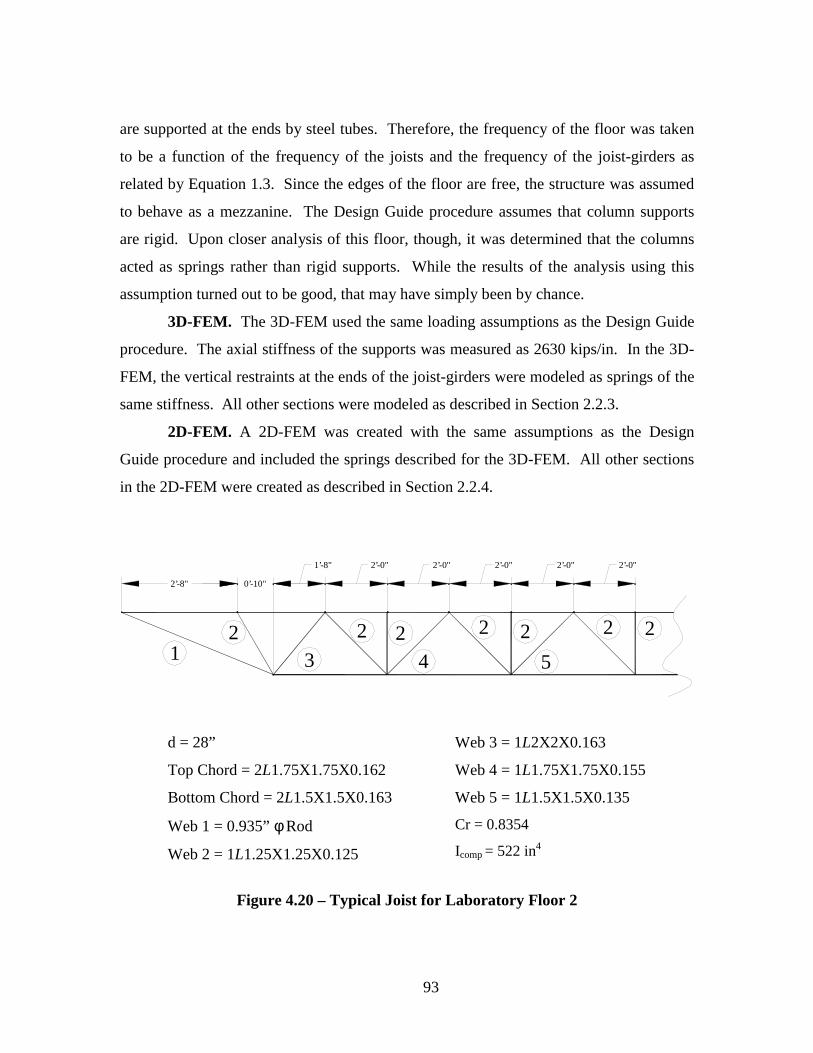
93
are supported at the ends by steel tubes. Therefore, the frequency of the floor was taken
to be a function of the frequency of the joists and the frequency of the joist-girders as
related by Equation 1.3. Since the edges of the floor are free, the structure was assumed
to behave as a mezzanine. The Design Guide procedure assumes that column supports
are rigid. Upon closer analysis of this floor, though, it was determined that the columns
acted as springs rather than rigid supports. While the results of the analysis using this
assumption turned out to be good, that may have simply been by chance.
3D-FEM. The 3D-FEM used the same loading assumptions as the Design Guide
procedure. The axial stiffness of the supports was measured as 2630 kips/in. In the 3D-
FEM, the vertical restraints at the ends of the joist-girders were modeled as springs of the
same stiffness. All other sections were modeled as described in Section 2.2.3.
2D-FEM. A 2D-FEM was created with the same assumptions as the Design
Guide procedure and included the springs described for the 3D-FEM. All other sections
in the 2D-FEM were created as described in Section 2.2.4.
2’-8" 0’-10"
1’-8" 2’-0" 2’-0" 2’-0" 2’-0"
12
3
2 24
2 2
5
2’-0"
2 2
d = 28”
Top Chord = 2L1.75X1.75X0.162
Bottom Chord = 2L1.5X1.5X0.163
Web 1 = 0.935” φ Rod
Web 2 = 1L1.25X1.25X0.125
Web 3 = 1L2X2X0.163
Web 4 = 1L1.75X1.75X0.155
Web 5 = 1L1.5X1.5X0.135
Cr = 0.8354
Icomp = 522 in4
Figure 4.20 – Typical Joist for Laboratory Floor 2
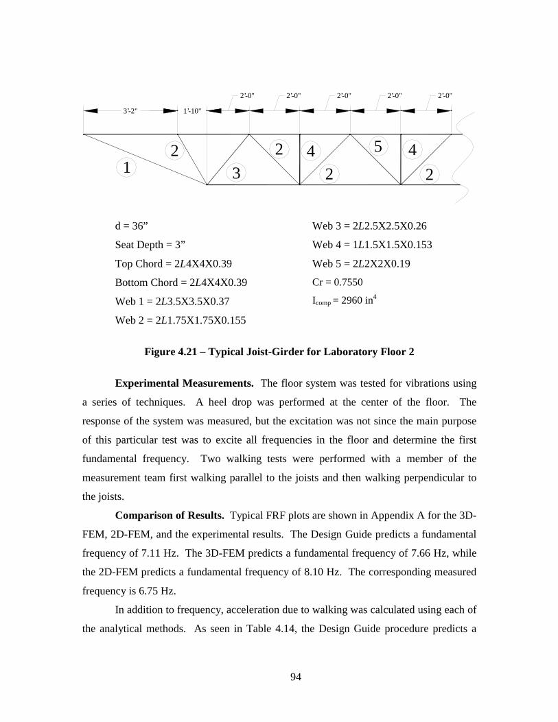
94
3’-2" 1’-10"
2’-0" 2’-0" 2’-0" 2’-0" 2’-0"
12
3
2 42
5 4
2
d = 36”
Seat Depth = 3”
Top Chord = 2L4X4X0.39
Bottom Chord = 2L4X4X0.39
Web 1 = 2L3.5X3.5X0.37
Web 2 = 2L1.75X1.75X0.155
Web 3 = 2L2.5X2.5X0.26
Web 4 = 1L1.5X1.5X0.153
Web 5 = 2L2X2X0.19
Cr = 0.7550
Icomp = 2960 in4
Figure 4.21 – Typical Joist-Girder for Laboratory Floor 2
Experimental Measurements. The floor system was tested for vibrations using
a series of techniques. A heel drop was performed at the center of the floor. The
response of the system was measured, but the excitation was not since the main purpose
of this particular test was to excite all frequencies in the floor and determine the first
fundamental frequency. Two walking tests were performed with a member of the
measurement team first walking parallel to the joists and then walking perpendicular to
the joists.
Comparison of Results. Typical FRF plots are shown in Appendix A for the 3D-
FEM, 2D-FEM, and the experimental results. The Design Guide predicts a fundamental
frequency of 7.11 Hz. The 3D-FEM predicts a fundamental frequency of 7.66 Hz, while
the 2D-FEM predicts a fundamental frequency of 8.10 Hz. The corresponding measured
frequency is 6.75 Hz.
In addition to frequency, acceleration due to walking was calculated using each of
the analytical methods. As seen in Table 4.14, the Design Guide procedure predicts a

95
peak walking acceleration of 4.83%g, the 3D-FEM predicts a peak walking acceleration
of 2.75%g, and the 2D-FEM predicts a peak walking acceleration of 2.86%g. The
measurement team record walking accelerations equal to 5%g for walking perpendicular
to the joists, and 4.9%g for walking parallel to the joists. The predicted walking
accelerations are all above the Design Guide recommended limit for human tolerance in
an office environment of 0.50%g. The measured accelerations are also above this same
limit. The subjective evaluation of the floor, by the measurement team, is that the floor
exhibits significant vibrations due to walking in its bare state.
In this case, both FEMs overestimated the fundamental frequency while the
Design Guide procedure came much closer. In terms of peak accelerations, again, the
Design Guide procedure was fairly accurate, while the 3D-FEM and the 2D-FEM were
well below the measured values.
Table 4.14Summary of Results for Laboratory Floor 2
Analysis Method
Parameter Design Guide 3D FiniteElement Model
2D FiniteElement Model
Measured Data
Frequency 7.11 Hz 7.66 Hz 8.10 Hz 6.75 Hz
p/g 4.83 %g 2.75 %g 2.86 %g // 5%g
⊥ 4.9%g
Acceptability Not Acceptable Not Acceptable Not Acceptable Not Acceptable

96
CHAPTER V
CONCLUSIONS AND RECCOMENDATIONS
5.1 INTRODUCTION
This study explored the ability of two finite element modeling techniques to
predict the fundamental frequency and peak acceleration of a variety of floors. Some of
these floors were constructed with lightweight concrete, while others were constructed
with normal weight concrete. Some floors were supported by joists, while others were
supported by hot-rolled beams. Each floor was loaded differently, and had a unique
damping ratio. The results from the finite element analyses were compared to predictions
from the Design Guide procedure and to experimental measurements.
5.2 CONCLUSIONS
Frequency. In general, as seen in Table 5.1, the prediction of the fundamental
frequency of a floor using either of the finite element techniques described earlier was
reliable. The 3D-FEM was used to predict the fundamental frequency of a floor
seventeen times, and correctly matched the measured frequency to within 0.5 Hz twelve
times. The 3D-FEM did not predict the correct frequency for Building 4 due to the fact
that the ballroom supports were more rigid than is generally assumed. The 3D-FEM did
not predict the correct frequency for Building 7 after the stiffening trusses were added,
due to the fact that the trusses stiffened the floor more than the model calculated. The
3D-FEM did not predict the correct frequency for Building 8, Area 2, for an unknown
reason. It is noted, though, that all three analyses for this particular floor were in error,
but were within 0.1 Hz of one another. The conclusion for this area is that the floor was
not constructed exactly as the plans indicated. The 3D-FEM did not predict the correct
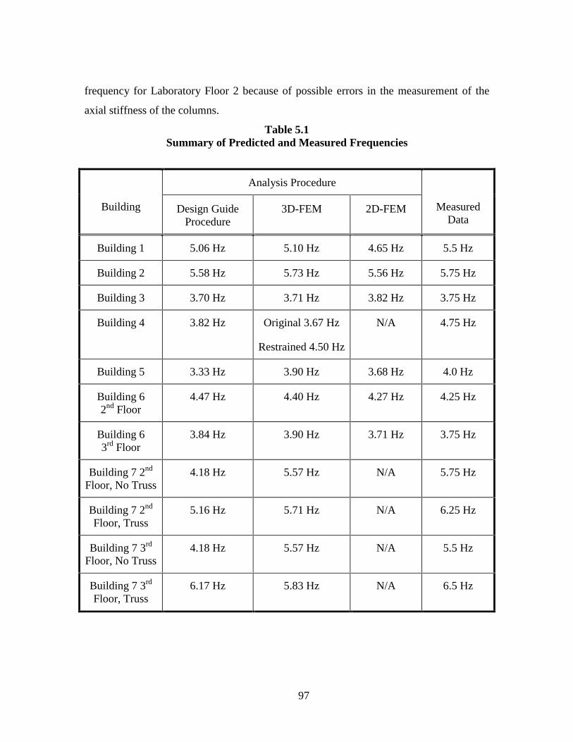
97
frequency for Laboratory Floor 2 because of possible errors in the measurement of the
axial stiffness of the columns.
Table 5.1Summary of Predicted and Measured Frequencies
Analysis Procedure
Building Design GuideProcedure
3D-FEM 2D-FEM MeasuredData
Building 1 5.06 Hz 5.10 Hz 4.65 Hz 5.5 Hz
Building 2 5.58 Hz 5.73 Hz 5.56 Hz 5.75 Hz
Building 3 3.70 Hz 3.71 Hz 3.82 Hz 3.75 Hz
Building 4 3.82 Hz Original 3.67 Hz
Restrained 4.50 Hz
N/A 4.75 Hz
Building 5 3.33 Hz 3.90 Hz 3.68 Hz 4.0 Hz
Building 62nd Floor
4.47 Hz 4.40 Hz 4.27 Hz 4.25 Hz
Building 63rd Floor
3.84 Hz 3.90 Hz 3.71 Hz 3.75 Hz
Building 7 2nd
Floor, No Truss4.18 Hz 5.57 Hz N/A 5.75 Hz
Building 7 2nd
Floor, Truss5.16 Hz 5.71 Hz N/A 6.25 Hz
Building 7 3rd
Floor, No Truss4.18 Hz 5.57 Hz N/A 5.5 Hz
Building 7 3rd
Floor, Truss6.17 Hz 5.83 Hz N/A 6.5 Hz

98
Table 5.1Summary of Predicted and Measured Frequencies (Continued)
Analysis Procedure
Building Design GuideProcedure
3D-FEM 2D-FEM MeasuredData
Building 8Area 1
7.41 Hz 8.59 Hz 8.63 Hz 9.0 Hz
Building 8Area 2
6.12 Hz 6.04 Hz 6.14 Hz 6.75 Hz
Building 9 N/A 2.65 Hz N/A 2.7 Hz
LaboratoryFloor 1
16.22 Hz 16.92 Hz 16.58 Hz 16.75 Hz
LaboratoryFloor 2
7.11 Hz 7.66 Hz 8.10 Hz 6.75 Hz
The 2D-FEM was used to predict the fundamental frequency of a floor ten times,
and correctly matched the measured frequency to within 0.5 Hz seven times. Two of the
analyses that were incorrect, for Building 8 and Laboratory Floor 2, were incorrect for the
same reasons as the 3D-FEM. The 2D-FEM did not predict the correct frequency for
Building 1 for an unknown reason.
The Design Guide procedure was used to predict the fundamental frequency of a
floor fifteen times, and correctly matched the measured frequency to within 0.5 Hz only
seven times. The analyses for Building 4 and Building 8, Area 2, were in error for the
same reasons as the 3D-FEM. The Design Guide procedure did not predict the correct
frequencies for Buildings 5 and 7, Building 8, Area 1, and Laboratory Floor 1 for
unknown reasons, since the FEMs used the same basic information and correctly
predicted the frequencies.
In general, the finite element modeling techniques did a better job of predicting
the fundamental frequency of a floor than did the most current design standard.

99
Peak Acceleration. In general, as shown in Table 5.2, the prediction of the peak
acceleration due to walking was unreliable. In almost all cases, the measured values for
walking were quite different from those predicted by any of the three analytical methods.
This discrepancy, though, was most likely due to the fact that the loads applied to the
models were not measured values, but instead were estimations of the force applied. All
three models, though, used the same loading, so it is disturbing that the 3D-FEM, 2D-
FEM and Design Guide procedure frequently predicted different walking accelerations
even when they predicted very similar frequencies. Clearly, the prediction of peak
accelerations is an area requiring more attention.
Table 5.2Summary of Predicted and Measured Peak Accelerations Due to Walking
Analysis Procedure
Building Design GuideProcedure
3D-FEM 2D-FEM Measured Data
Building 1 0.30 %g 0.41 %g 0.73 %g 1 %g – 2 %g
Building 2 1.24 %g 0.67 %g 0.75 %g 1.5 %g – 2.3 %g
Building 3 1.11 %g 0.46 %g 0.49 %g 6.4 %g – 7.7 %g
Building 4 0.12 %g Original 0.10 %gRestrained 0.09 %g
N/A N/A
Building 5 0.77 %g 0.37 %g 0.85 %g 2 %g – 3 %g
Building 62nd Floor
1.12 %g 0.80 %g 0.66 %g 0.8 %g
Building 63rd Floor
1.28 %g 0.92 %g 0.92 %g N/A
Building 72nd Floor,No Truss
0.95 %g 1.50 %g N/A 2.1 %g – 3.6 %g

100
Table 5.2Summary of Predicted and Measured Peak Accelerations Due to Walking
(Continued)
Analysis Procedure
Building Design GuideProcedure
3D-FEM 2D-FEM Measured Data
Building 7 2nd
Floor, Truss0.70 %g 1.27 %g N/A 0.5 %g – 2.2 %g
Building 7 3rd
Floor, No Truss0.95 %g 1.50 %g N/A 2.5 %g – 2.7 %g
Building 7 3rd
Floor, Truss0.52 %g 1.10 %g N/A 1.4 %g – 1.9 %g
Building 8Area 1
0.97 %g 0.75 %g 0.88 %g 0.9 %g – 2.5 %g
Building 8Area 2
0.89 %g 0.41 %g 1.28 %g 0.7 %g – 1.2 %g
Building 9 N/A N/A N/A N/A
LaboratoryFloor 1
0.19 %g 0.06 %g 0.10 %g 0.04 %g – 0.05 %g
LaboratoryFloor 2
4.83 %g 2.75 %g 2.86 %g 4.90 %g - 5.00 %g
5.3 RECOMMENDATIONS FOR FUTURE RESEARCH
This study has shown that the finite element modeling techniques described are
capable of accurately predicting the first fundamental frequency of a floor, but are
generally not capable of accurately predicting the actual peak acceleration response of a
floor due to a dynamic load. Some possible areas of future research are presented here,
along with the recommendations of this study.

101
Non-Structural Components. The effect of non-structural components on the
vibration characteristics of a real floor needs to be studied. Non-structural components
can serve to both dampen and stiffen a floor. Their contribution is generally neglected in
both the equations presented in the Design Guide and in the finite element modeling
techniques.
Effective Mass. The effective mass of a real floor needs to be determined
experimentally. The effective mass is inversely proportional to the acceleration response
of the system. Clearly, from the results of this study, the effective mass calculated for a
system in the Design Guide procedure is very different from the equivalent effective
mass in a finite element model since different peak accelerations are predicted for the
same floor even when the same frequency is predicted. A study needs to be undertaken
to determine the actual percentage of mass that is generally effective in a real building.
Continuity. The effect of continuity needs to be examined. An underlying
assumption in the Design Guide is that a series of bays can be modeled as a single bay.
In the finite element models, though, adjacent bays can serve to stiffen a bay and thus
change its behavior. How accurate these assumptions are for real buildings needs to be
determined.
Acceleration Response. It is recommended that future research concentrate on
measuring both the force input and response of a structure for a dynamic load. Since
reality is the true measuring stick here, comparing the finite element results to the Design
Guide results is of little value if the Design Guide results are in error.
Transient Nature of Walking. It is also recommended that the transient nature
of walking be examined and included as a parameter in future studies. It is a simple
matter to apply a transient load to a finite element model, and it may, perhaps, yield more
accurate results.

102
LIST OF REFERENCES
Allen, D. E. (1990). “Building Vibrations from Human Activities.” ConcreteInternational, American Concrete Institute, Detroit, Michigan, pp. 66-73.
Allen, D. E., and Murray, T. M. (1993). “Design Criterion for Vibrations Due toWalking.” Engineering Journal, AISC, Chicago, Illinois, pp. 117-129.
Allen, D. E., and Ranier, J. H. (1976). “Vibration Criteria for Long-Span Floors.”Canadian Journal of Civil Engineering, NRCC, Ottawa, Ontario, Canada, pp.165-173.
Band B. S. Jr. (1996). “Several Vibration Performance Aspects of Joist and Joist-GirderSupported Floors.” M.S. Thesis, Virginia Polytechnic Institute and StateUniversity, Blacksburg, Virginia.
Beavers, T. A. (1998). “Fundamental Natural Frequency of Steel Joist-SupportedFloors.” M.S. Thesis, Virginia Polytechnic Institute and State University,Blacksburg, Virginia.
Biggs, J. M. (1964). Introduction to Structural Dynamics, McGraw-Hill, New York,New York.
CSA, 1989, Canadian Standards CAN3-S16.1-M89: Steel Structures for Buildings –Limit States Design: Appendix G, Guide for Floor Vibrations. Ontario, Canada.
Hanagan, L. M. (1994). “Active Control of Floor Vibrations.” Ph.D. Dissertation,Virginia Polytechnic Institute and State University, Blacksburg, Virginia.
International Standards Organization (1989). “Evaluation of Human Exposure toContinuous and Shock-Induced Vibrations in Buildings.” International Standard,ISO 2631-2.
Kitterman, S. S. (1994). “Investigation of Several Aspects of the VibrationCharacteristics of Steel Member-Supported Floors.” M.S. Thesis, VirginiaPolytechnic Institute and State University, Blacksburg, Virginia.
Lenzen, K. H. (1966). “Vibration of Steel Joist-Concrete Slab Floors.” EngineeringJournal, AISC, Chicago, Illinois, pp. 133-136.
Murray, T. M. (1975). “Design to Prevent Floor Vibrations.” Engineering Journal,AISC, Chicago, Illinois, pp. 82-87.
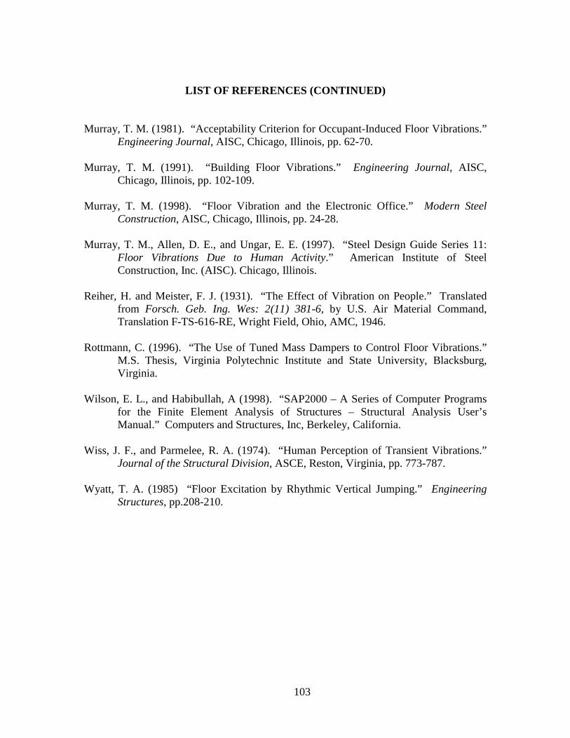
103
LIST OF REFERENCES (CONTINUED)
Murray, T. M. (1981). “Acceptability Criterion for Occupant-Induced Floor Vibrations.”Engineering Journal, AISC, Chicago, Illinois, pp. 62-70.
Murray, T. M. (1991). “Building Floor Vibrations.” Engineering Journal, AISC,Chicago, Illinois, pp. 102-109.
Murray, T. M. (1998). “Floor Vibration and the Electronic Office.” Modern SteelConstruction, AISC, Chicago, Illinois, pp. 24-28.
Murray, T. M., Allen, D. E., and Ungar, E. E. (1997). “Steel Design Guide Series 11:Floor Vibrations Due to Human Activity.” American Institute of SteelConstruction, Inc. (AISC). Chicago, Illinois.
Reiher, H. and Meister, F. J. (1931). “The Effect of Vibration on People.” Translatedfrom Forsch. Geb. Ing. Wes: 2(11) 381-6, by U.S. Air Material Command,Translation F-TS-616-RE, Wright Field, Ohio, AMC, 1946.
Rottmann, C. (1996). “The Use of Tuned Mass Dampers to Control Floor Vibrations.”M.S. Thesis, Virginia Polytechnic Institute and State University, Blacksburg,Virginia.
Wilson, E. L., and Habibullah, A (1998). “SAP2000 – A Series of Computer Programsfor the Finite Element Analysis of Structures – Structural Analysis User’sManual.” Computers and Structures, Inc, Berkeley, California.
Wiss, J. F., and Parmelee, R. A. (1974). “Human Perception of Transient Vibrations.”Journal of the Structural Division, ASCE, Reston, Virginia, pp. 773-787.
Wyatt, T. A. (1985) “Floor Excitation by Rhythmic Vertical Jumping.” EngineeringStructures, pp.208-210.

104
Appendix A
FRF Plots and Acceleration Traces

105
5
0
20
40
60
80
100
0 5 10 15 20 25 30
FREQUENCY (HZ)a) 3D-FEM
AM
PL
ITU
DE
4.75
0
500
1000
1500
2000
2500
3000
3500
0 5 10 15 20 25 30
FREQUENCY (HZ)b) 2D-FEM
AM
PL
ITU
DE
5.5
00.0005
0.0010.0015
0.0020.0025
0.0030.0035
0.004
0 5 10 15 20 25 30
FREQUENCY (HZ)c) Measured Data From Heel Drop
AM
PL
ITU
DE
Figure A.1 – FRF Plots for Building 1

106
-1.5
-1
-0.5
0
0.5
1
1.5
0 1 2 3 4
TIME (s)a) Walking Parallel to the Beams
AC
CE
LE
RA
TIO
N (%
g)
-1.5
-1
-0.5
0
0.5
1
1.5
0 1 2 3 4
TIME (s)b) Walking in Place (40 Steps in 15 Sec.)
AC
CE
LE
RA
TIO
N (%
g)
Figure A.2 – Measured Accelerations for Building 1

107
-0.08
-0.06
-0.04
-0.02
0
0.02
0.04
0.06
0.08
0 1 2 3 4
TIME (s)c) Ambient Vibration
AC
CE
LE
RA
TIO
N (%
g)
-2.5
-2
-1.5
-1
-0.5
0
0.5
1
1.5
2
2.5
0 1 2 3 4
TIME (s)d) Rhythmic Excitation
AC
CE
LE
RA
TIO
N (%
g)
Figure A.2 – Measured Accelerations for Building 1 (Continued)

108
5.75
0
200
400
600
800
1000
1200
0 5 10 15 20 25 30
FREQUENCY (HZ)a) 3D-FEM
AM
PL
ITU
DE
5.5
0
200
400
600
800
1000
1200
1400
0 5 10 15 20 25 30
FREQUENCY (HZ)
b) 2D-FEM
AM
PL
ITU
DE
Figure A.3 –FRF Plots for Building 2
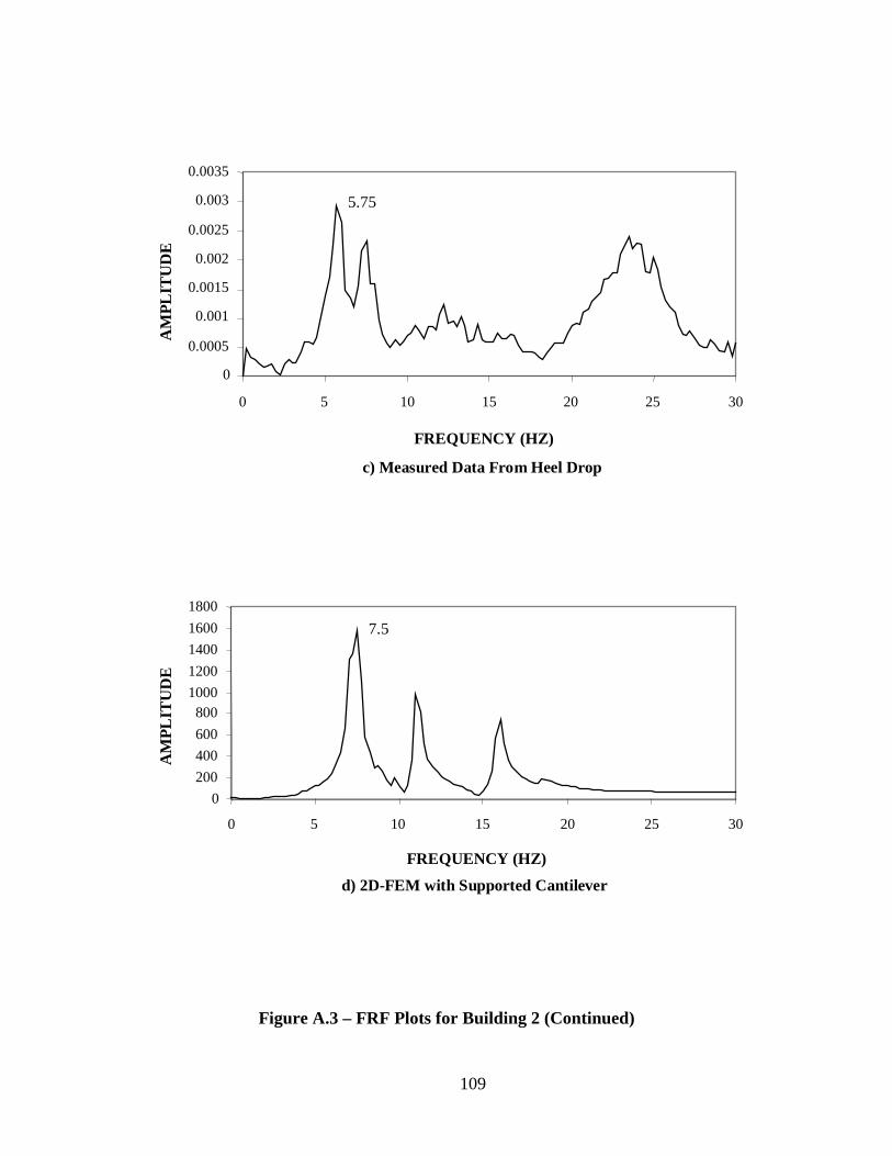
109
5.75
0
0.0005
0.001
0.0015
0.002
0.0025
0.003
0.0035
0 5 10 15 20 25 30
FREQUENCY (HZ)
c) Measured Data From Heel Drop
AM
PL
ITU
DE
7.5
0
200
400
600
8001000
1200
1400
1600
1800
0 5 10 15 20 25 30
FREQUENCY (HZ)
d) 2D-FEM with Supported Cantilever
AM
PL
ITU
DE
Figure A.3 – FRF Plots for Building 2 (Continued)
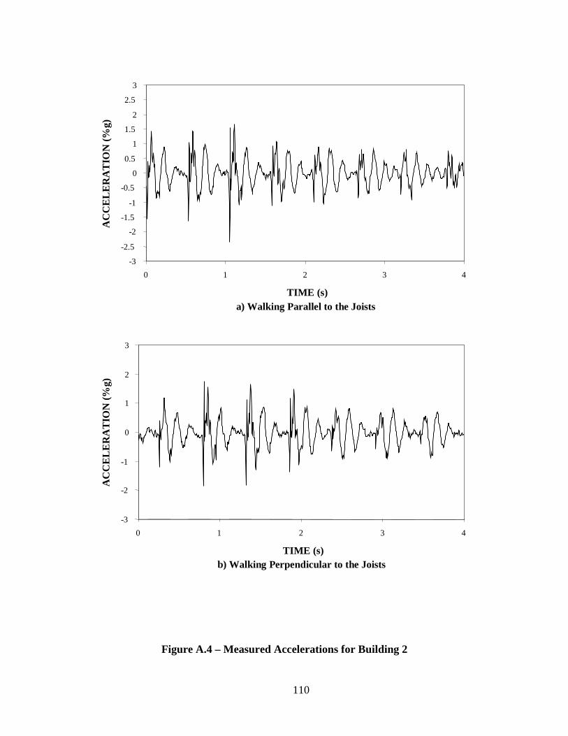
110
-3
-2.5
-2
-1.5
-1
-0.5
0
0.5
1
1.5
2
2.5
3
0 1 2 3 4
TIME (s)a) Walking Parallel to the Joists
AC
CE
LE
RA
TIO
N (%
g)
-3
-2
-1
0
1
2
3
0 1 2 3 4
TIME (s)b) Walking Perpendicular to the Joists
AC
CE
LE
RA
TIO
N (%
g)
Figure A.4 – Measured Accelerations for Building 2

111
-3
-2
-1
0
1
2
3
0 1 2 3 4
TIME (s)
c) Rhythmic Excitation
AC
CE
LE
RA
TIO
N (%
g)
Figure A.4 – Measured Accelerations for Building 2 (Continued)

112
5
3.75
0
10
20
30
40
50
60
70
0 5 10 15 20 25 30
FREQUENCY (HZ)a) 3D-FEM
AM
PL
ITU
DE
6
4.25
3.75
0
500
1000
1500
2000
2500
30003500
4000
0 5 10 15 20 25 30
FREQUENCY (HZ)b) 2D-FEM
AM
PL
ITU
DE
3.75
0
0.5
1
1.5
2
0 5 10 15 20 25 30
FREQUENCY (HZ)c) Measured Data From Heel Drop
AM
PL
ITU
DE
Figure A.5 – FRF Plots for Building 3
113
-10
-7.5
-5
-2.5
0
2.5
5
7.5
10
0 1 2 3 4
TIME (s)
a) Walking Parallel to the Joists
AC
CE
LE
RA
TIO
N (%
g)
-10
-7.5
-5
-2.5
0
2.5
5
7.5
10
0 1 2 3 4
TIME (s)b) Walking Perpendicular to the Joists
AC
CE
LE
RA
TIO
N (%
g)
Figure A.6 –Measured Accelerations for Building 3

114
-40
-30
-20
-10
0
10
20
30
40
0 1 2 3 4
TIME (s)c) Walking in Place (48 Steps in 15 Sec.)
AC
CE
LE
RA
TIO
N (%
g)
Figure A.6 –Measured Accelerations for Building 3 (Continued)
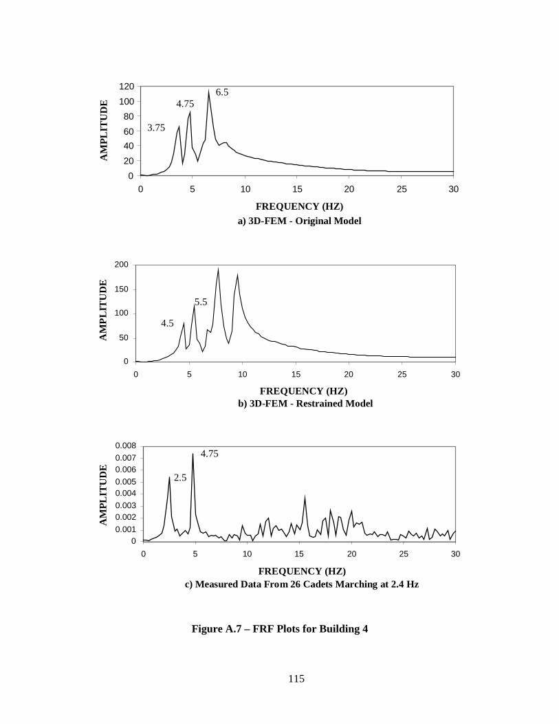
115
4.756.5
3.75
0
20
40
60
80
100
120
0 5 10 15 20 25 30
FREQUENCY (HZ)a) 3D-FEM - Original Model
AM
PL
ITU
DE
5.5
4.5
0
50
100
150
200
0 5 10 15 20 25 30
FREQUENCY (HZ)b) 3D-FEM - Restrained Model
AM
PL
ITU
DE
2.5
4.75
00.001
0.0020.003
0.0040.005
0.0060.007
0.008
0 5 10 15 20 25 30
FREQUENCY (HZ)c) Measured Data From 26 Cadets Marching at 2.4 Hz
AM
PL
ITU
DE
Figure A.7 – FRF Plots for Building 4

116
-10
-8
-6
-4
-2
0
2
4
6
8
10
0 0.5 1 1.5 2 2.5 3 3.5 4
TIME (s)a) 26 Cadets Marching, 144 Beats per Minute = 2.4 Hz
AC
CE
LE
RA
TIO
N (%
g)
-10
-8
-6
-4
-2
0
2
4
6
8
10
0 0.5 1 1.5 2 2.5 3 3.5 4
TIME (s)b) 17 Cadets Marching, 144 Beats per Minute = 2.4 Hz
AC
CE
LE
RA
TIO
N (%
g)
Figure A.8 – Measured Accelerations for Building 4

117
-10
-8
-6
-4
-2
0
2
4
6
8
10
0 0.5 1 1.5 2 2.5 3 3.5 4
TIME (s)c) 70 Students Dancing
AC
CE
LE
RA
TIO
N (%
g)
Figure A.8 – Measured Accelerations for Building 4 (Continued)

118
3.75
4.5
0
500
1000
1500
2000
2500
3000
0 5 10 15 20 25 30
FREQUENCY (HZ)a) 3D-FEM
AM
PL
ITU
DE
3.75
0
500
1000
1500
2000
2500
0 5 10 15 20 25 30
FREQUENCY (HZ)b) 2D-FEM
AM
PL
ITU
DE
4
0
0.001
0.002
0.003
0.004
0.005
0 5 10 15 20 25 30
FREQUENCY (HZ)c) Measured Data From Heel Drop
AM
PL
ITU
DE
Figure A.9 – FRF Plots for Building 5

119
-3
-2
-1
0
1
2
3
0 0.5 1 1.5 2 2.5 3 3.5 4
TIME (s)a) Walking Parallel to the Beams
AC
CE
LE
RA
TIO
N (
%g)
-3
-2
-1
0
1
2
3
0 0.5 1 1.5 2 2.5 3 3.5 4
TIME (s)b) Walking Perpendicular to the Beams
AC
CE
LE
RA
TIO
N (
%g)
Figure A.10 –Measured Accelerations for Building 5

120
-10
-6
-2
2
6
10
0 0.5 1 1.5 2 2.5 3 3.5 4
TIME (s)c) Walking in Place (34 Steps in 15 Sec.)
AC
CE
LE
RA
TIO
N (%
g)
Figure A.10 –Measured Accelerations for Building 5 (Continued)

121
4.75
4.25
0
500
1000
1500
2000
2500
3000
3500
0 5 10 15 20 25 30
FREQUENCY (HZ)
a) 3D-FEM - 2nd Floor
AM
PL
ITU
DE
4.5
0
500
1000
1500
2000
2500
3000
0 5 10 15 20 25 30
FREQUENCY (HZ)b) 2D-FEM - 2nd Floor
AM
PL
ITU
DE
Figure A.11 – FRF Plots for Building 6
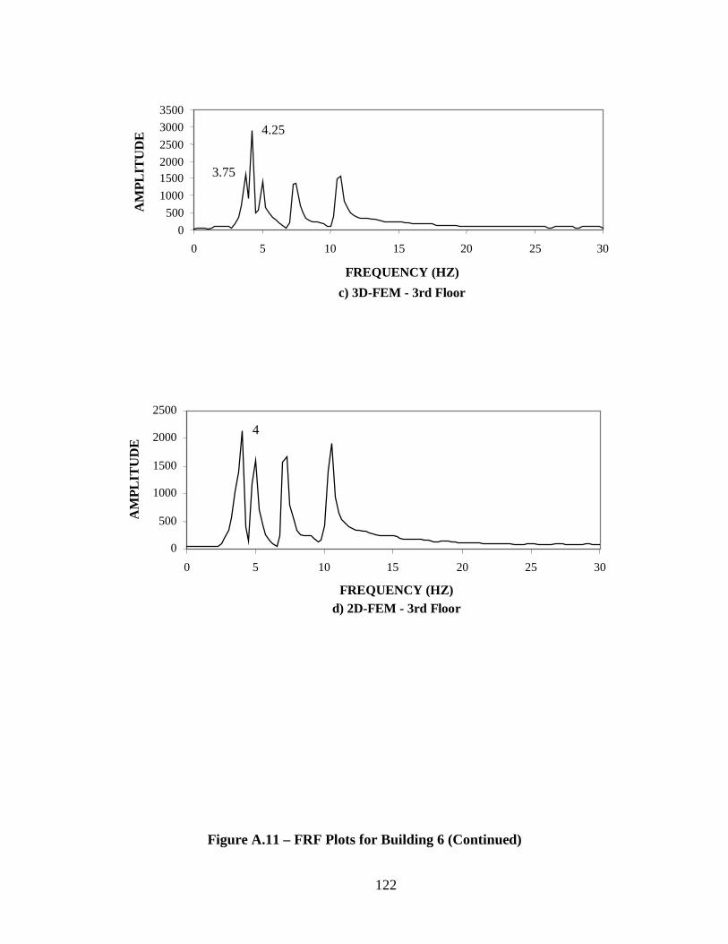
122
4.25
3.75
0
500
1000
15002000
2500
3000
3500
0 5 10 15 20 25 30
FREQUENCY (HZ)
c) 3D-FEM - 3rd Floor
AM
PL
ITU
DE
4
0
500
1000
1500
2000
2500
0 5 10 15 20 25 30
FREQUENCY (HZ)d) 2D-FEM - 3rd Floor
AM
PL
ITU
DE
Figure A.11 – FRF Plots for Building 6 (Continued)
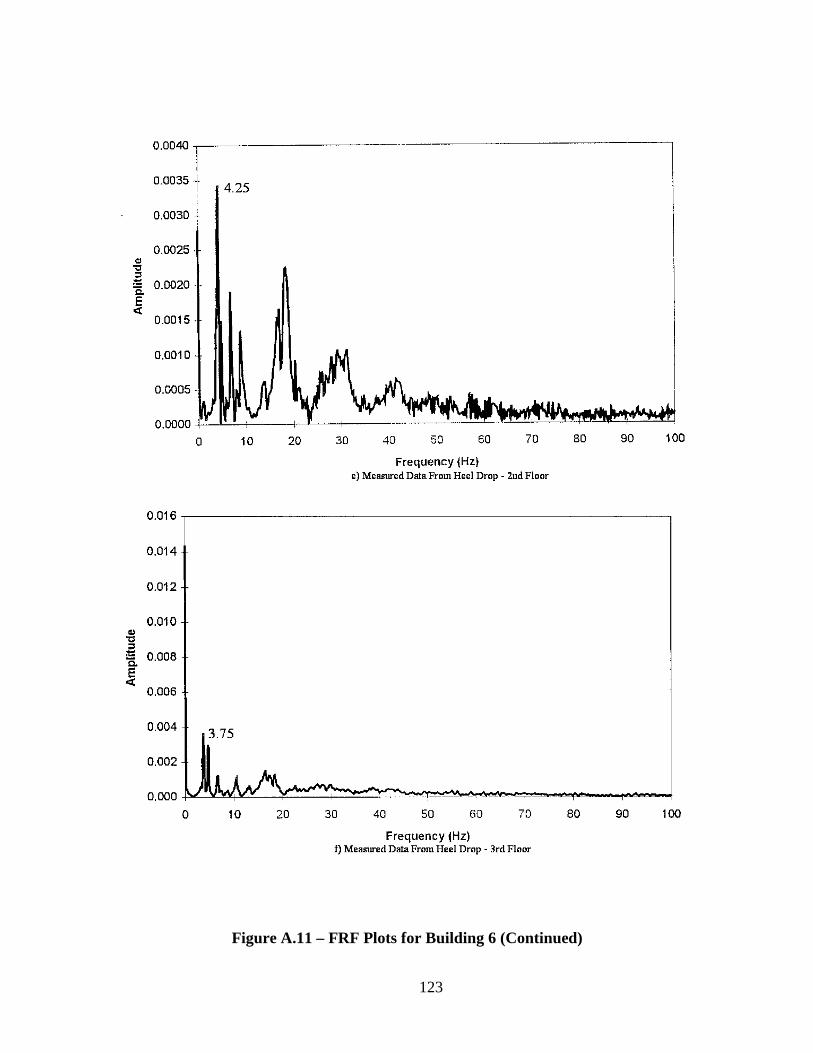
123
Figure A.11 – FRF Plots for Building 6 (Continued)
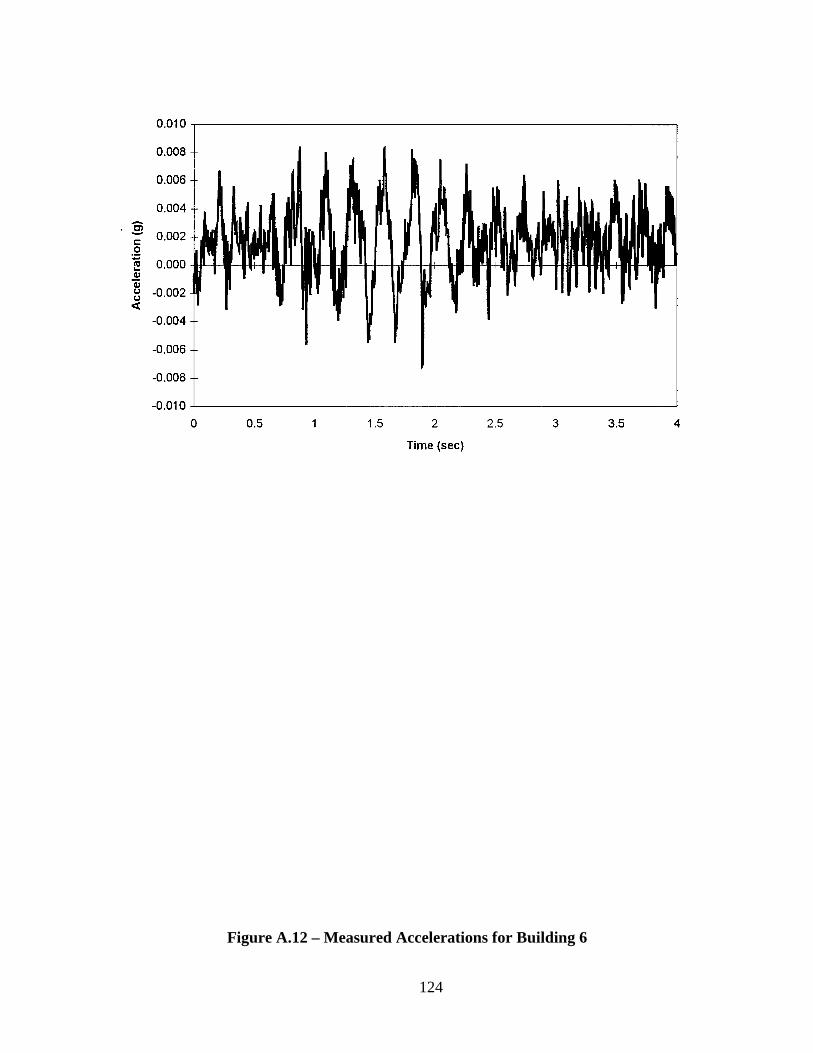
124
Figure A.12 – Measured Accelerations for Building 6

125
5.5
0
2000
4000
6000
8000
10000
0 5 10 15 20 25 30
FREQUENCY (HZ)
a) 3D-FEM - 2nd Floor No Truss
AM
PL
ITU
DE
5.75
0
0.005
0.01
0.015
0.02
0 5 10 15 20 25 30
FREQUENCY (HZ)b) Measured Data From Heel Drop
2nd Floor No Truss
AM
PL
ITU
DE
Figure A.13 – FRF Plots for Building 7

126
5.75
0
100020003000
4000
5000
6000
7000
8000
0 5 10 15 20 25 30
FREQUENCY (HZ)c) 3D-FEM - 2nd Floor With Truss
AM
PL
ITU
DE
6.25
0
0.002
0.004
0.006
0.008
0 5 10 15 20 25 30
FREQUENCY (HZ)
d) Measured Data From Heel Drop
2nd Floor With Truss
AM
PL
ITU
DE
Figure A.13 – FRF Plots for Building 7 (Continued)

127
5.5
0
2000
4000
6000
8000
10000
0 5 10 15 20 25 30
FREQUENCY (HZ)
e) 3D-FEM - 3rd Floor No Truss
AM
PL
ITU
DE
5.5
0
0.005
0.01
0.015
0 5 10 15 20 25 30
FREQUENCY (HZ)f) Measured Data From Heel Drop
3rd Floor No Truss
AM
PL
ITU
DE
Figure A.13 – FRF Plots for Building 7 (Continued)

128
5.75
0
1000
2000
3000
4000
5000
6000
7000
8000
0 5 10 15 20 25 30
FREQUENCY (HZ)g) 3D-FEM - 3rd Floor With Truss
AM
PL
ITU
DE
6.5
0
0.002
0.004
0.006
0.008
0 5 10 15 20 25 30
FREQUENCY (HZ)h) Measured Data From Heel Drop
3rd Floor With Truss
AM
PL
ITU
DE
Figure A.13 – FRF Plots for Building 7 (Continued)

129
-4
-3
-2
-1
0
1
2
3
4
5
0 0.5 1 1.5 2 2.5 3 3.5 4
TIME (s)a) Walking Parallel to the Beams
No Truss - 2nd Floor
AC
CE
LE
RA
TIO
N (
%g)
-5
-4
-3
-2
-1
0
1
2
3
4
5
0 0.5 1 1.5 2 2.5 3 3.5 4
TIME (s)b) Walking Perpendicular to the Beams
No Truss - 2nd Floor
AC
CE
LE
RA
TIO
N (
%g)
Figure A.14 – Measured Accelerations for Building 7

130
-5
-4
-3
-2
-1
0
1
2
3
4
5
0 0.5 1 1.5 2 2.5 3 3.5 4
TIME (s)c) Walking Parallel to the Beams
With Truss - 2nd Floor
AC
CE
LE
RA
TIO
N (
%g)
-5
-4
-3
-2
-1
0
1
2
3
4
5
0 0.5 1 1.5 2 2.5 3 3.5 4
TIME (s)d) Walking Perpendicular to the Beams
With Truss - 2nd Floor
AC
CE
LE
RA
TIO
N (%
g)
Figure A.14 – Measured Accelerations for Building 7 (Continued)

131
-5
-4
-3
-2
-1
0
1
2
3
4
5
0 0.5 1 1.5 2 2.5 3 3.5 4
TIME (s)
e) Walking Parallel to the BeamsNo Truss - 3rd Floor
AC
CE
LE
RA
TIO
N (%
g)
-5
-4
-3
-2
-1
0
1
2
3
4
5
0 0.5 1 1.5 2 2.5 3 3.5 4
TIME (s)f) Walking Perpendicular to the Beams
No Truss - 3rd Floor
AC
CE
LE
RA
TIO
N (%
g)
Figure A.14 – Measured Accelerations for Building 7 (Continued)
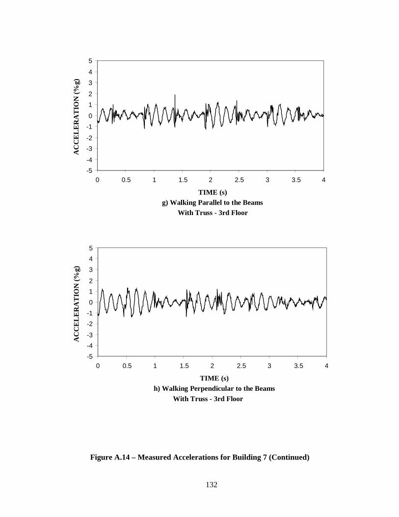
132
-5
-4
-3
-2
-1
0
1
2
3
4
5
0 0.5 1 1.5 2 2.5 3 3.5 4
TIME (s)g) Walking Parallel to the Beams
With Truss - 3rd Floor
AC
CE
LE
RA
TIO
N (%
g)
-5
-4
-3
-2
-1
0
1
2
3
4
5
0 0.5 1 1.5 2 2.5 3 3.5 4
TIME (s)h) Walking Perpendicular to the Beams
With Truss - 3rd Floor
AC
CE
LE
RA
TIO
N (%
g)
Figure A.14 – Measured Accelerations for Building 7 (Continued)

133
8.5
0
500
1000
1500
2000
2500
3000
0 5 10 15 20 25 30
FREQUENCY (HZ)a) 3D-FEM - 1st Area
AM
PL
ITU
DE
8.75
0
2
4
6
8
10
0 5 10 15 20 25 30
FREQUENCY (HZ)b) 2D-FEM - 1st Area
AM
PL
ITU
DE
9
0
0.001
0.002
0.003
0.004
0.005
0 5 10 15 20 25 30
FREQUENCY (HZ)c) Measured Data From Heel Drop - 1st Area
AM
PL
ITU
DE
Figure A.15 – FRF Plots for Building 8
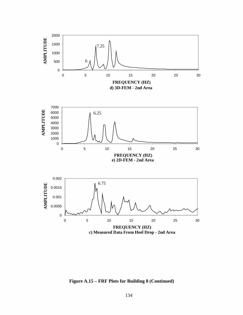
134
7.25
6
0
500
1000
1500
2000
0 5 10 15 20 25 30
FREQUENCY (HZ)d) 3D-FEM - 2nd Area
AM
PL
ITU
DE
6.25
0
10002000
30004000
50006000
7000
0 5 10 15 20 25 30
FREQUENCY (HZ)e) 2D-FEM - 2nd Area
AM
PL
ITU
DE
6.75
0
0.0005
0.001
0.0015
0.002
0 5 10 15 20 25 30
FREQUENCY (HZ)c) Measured Data From Heel Drop - 2nd Area
AM
PL
ITU
DE
Figure A.15 – FRF Plots for Building 8 (Continued)

135
-3
-2
-1
0
1
2
3
0 0.5 1 1.5 2 2.5 3 3.5 4
TIME (s)a) Walking Parallel to the Joists - 1st Area
AC
CE
LE
RA
TIO
N (%
g)
-3
-2
-1
0
1
2
3
0 0.5 1 1.5 2 2.5 3 3.5 4
TIME (s)b) Walking Perpendicular to the Joists - 1st Area
AC
CE
LE
RA
TIO
N (%
g)
Figure A.16 – Measured Accelerations for Building 8
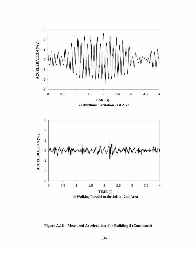
136
-3
-2
-1
0
1
2
3
0 0.5 1 1.5 2 2.5 3 3.5 4
TIME (s)c) Rhythmic Excitation - 1st Area
AC
CE
LE
RA
TIO
N (%
g)
-3
-2
-1
0
1
2
3
0 0.5 1 1.5 2 2.5 3 3.5 4
TIME (s)d) Walking Parallel to the Joists - 2nd Area
AC
CE
LE
RA
TIO
N (%
g)
Figure A.16 – Measured Accelerations for Building 8 (Continued)

137
-3
-2
-1
0
1
2
3
0 0.5 1 1.5 2 2.5 3 3.5 4
TIME (s)f) Walking Perpendicular to the Joists - 2nd Area
AC
CE
LE
RA
TIO
N (%
g)
-3
-2
-1
0
1
2
3
0 0.5 1 1.5 2 2.5 3 3.5 4
TIME (s)f) Rhythmic Excitation - 2nd Area
AC
CE
LE
RA
TIO
N (%
g)
Figure A.16 – Measured Accelerations for Building 8 (Continued)

138
16.75
17.5
0
2000
4000
6000
8000
10000
12000
0 5 10 15 20 25 30
FREQUENCY (HZ)
a) 3D-FEM
AM
PL
ITU
DE
16.5
0
2000
4000
6000
8000
10000
12000
14000
0 5 10 15 20 25 30
FREQUENCY (HZ)b) 2D-FEM - I Measured
AM
PL
ITU
DE
Figure A.17 – FRF Plots for Laboratory Floor 1
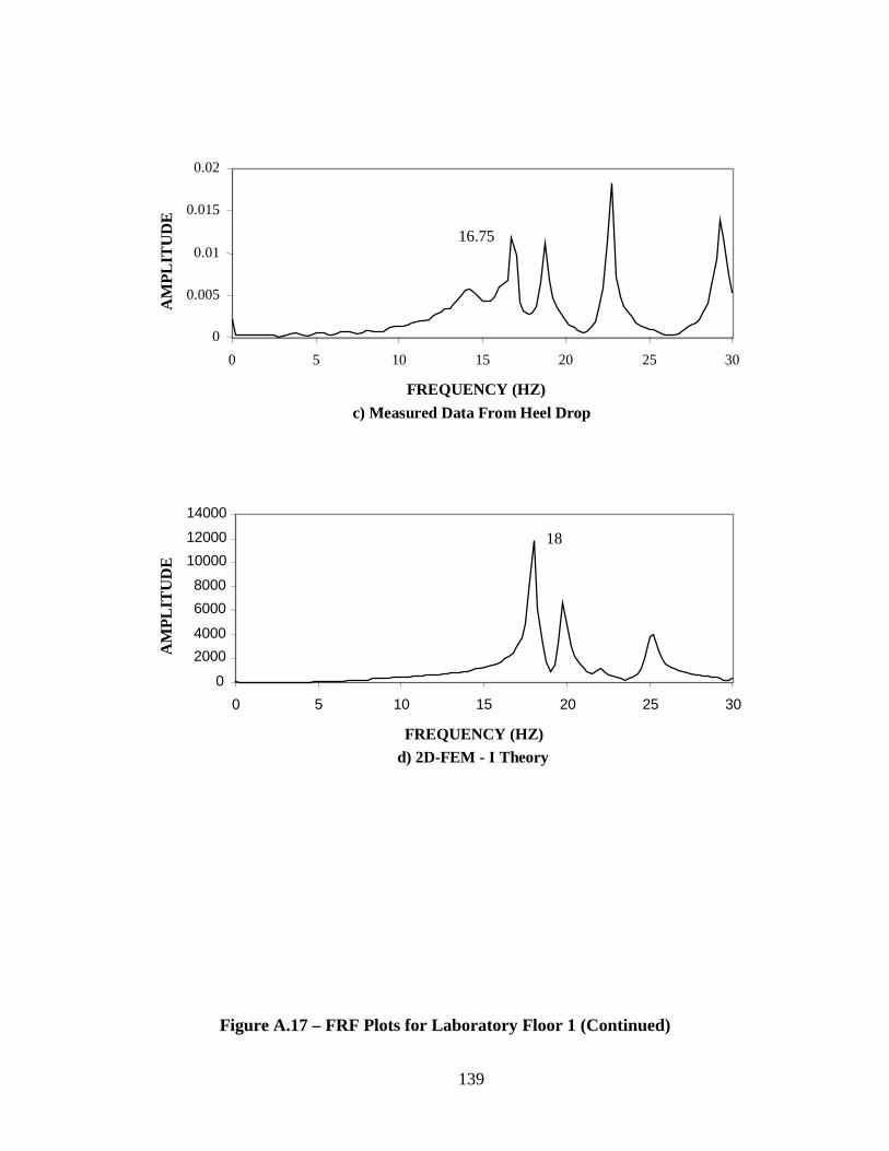
139
16.75
0
0.005
0.01
0.015
0.02
0 5 10 15 20 25 30
FREQUENCY (HZ)
c) Measured Data From Heel Drop
AM
PL
ITU
DE
18
0
2000
4000
6000
8000
10000
12000
14000
0 5 10 15 20 25 30
FREQUENCY (HZ)
d) 2D-FEM - I Theory
AM
PL
ITU
DE
Figure A.17 – FRF Plots for Laboratory Floor 1 (Continued)

140
-0.1
-0.05
0
0.05
0.1
0 0.5 1 1.5 2 2.5 3 3.5 4
TIME (s)a) Walking Parallel to the Joists
AC
CE
LE
RA
TIO
N (%
g)
-0.1
-0.05
0
0.05
0.1
0 0.5 1 1.5 2 2.5 3 3.5 4
TIME (s)b) Walking Perpendicular to the Joists
AC
CE
LE
RA
TIO
N (%
g)
Figure A.18 – Measured Accelerations for Laboratory Floor 1

141
-0.25
-0.2
-0.15
-0.1
-0.05
0
0.05
0.1
0.15
0.2
0.25
0 0.5 1 1.5 2 2.5 3 3.5 4
TIME (s)c) Walking in Place (43 Steps in 15 Sec.)
AC
CE
LE
RA
TIO
N (
%g)
Figure A.18 – Measured Accelerations for Laboratory Floor 1 (Continued)

142
7.5
0
1000
2000
3000
4000
5000
6000
0 5 10 15 20 25 30
FREQUENCY (HZ)a) 3D-FEM
AM
PL
ITU
DE
8.5
1000
3000
5000
7000
9000
0 5 10 15 20 25 30
FREQUENCY (HZ)b) 2D-FEM
AM
PL
ITU
DE
6.75
0
0.005
0.01
0.015
0.02
0.025
0.03
0.035
0 5 10 15 20 25 30
FREQUENCY (HZ)c) Measured Data From Heel Drop
AM
PL
ITU
DE
Figure A.19 – FRF Plots for Laboratory Floor 2

143
-6
-4
-2
0
2
4
6
0 0.5 1 1.5 2 2.5 3 3.5 4
TIME (s)a) Walking Parallel to the Joists
AC
CE
LE
RA
TIO
N (%
g)
-6
-4
-2
0
2
4
6
0 0.5 1 1.5 2 2.5 3 3.5 4
TIME (s)b) Walking Perpendicular to the Joists
AC
CE
LE
RA
TIO
N (%
g)
Figure A.20 – Measured Accelerations for Laboratory Floor 2

144
Appendix B
Finite Element Modeling Techniques
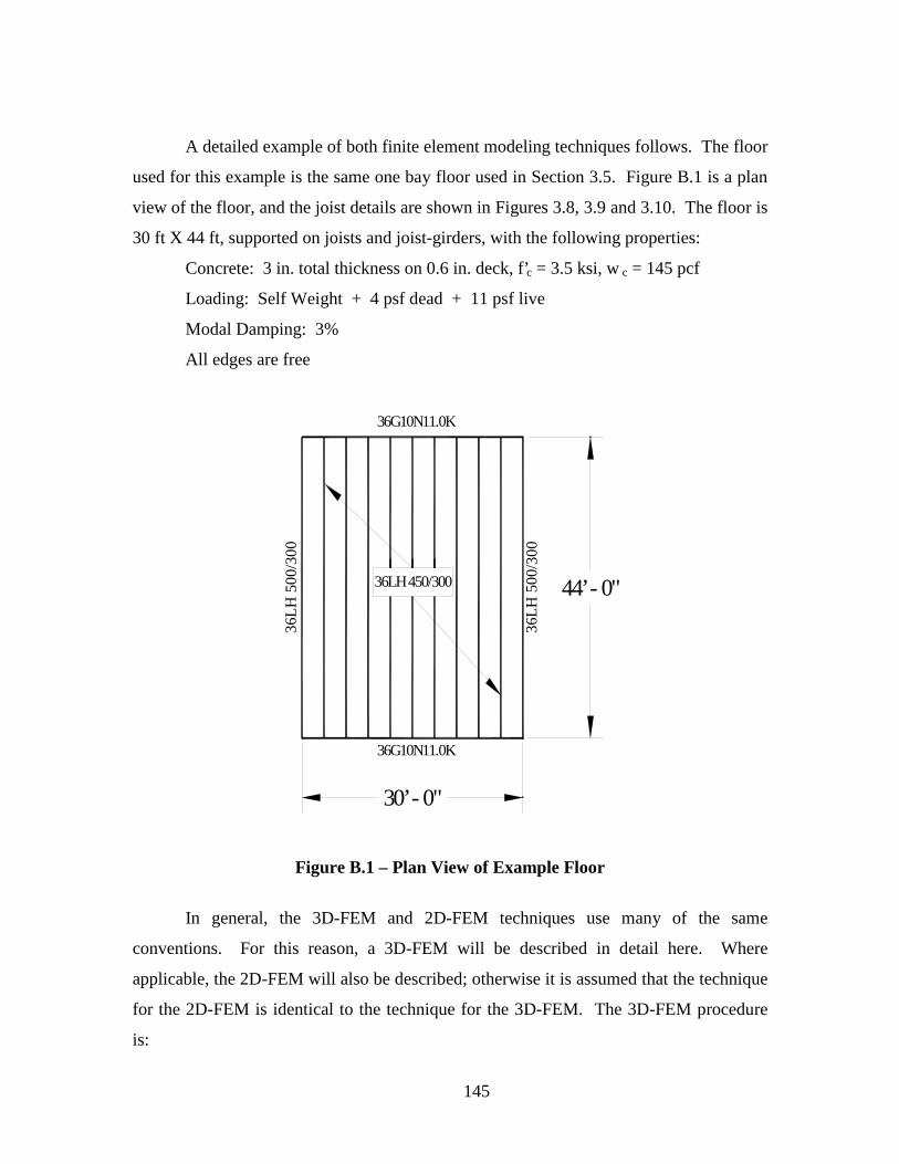
145
A detailed example of both finite element modeling techniques follows. The floor
used for this example is the same one bay floor used in Section 3.5. Figure B.1 is a plan
view of the floor, and the joist details are shown in Figures 3.8, 3.9 and 3.10. The floor is
30 ft X 44 ft, supported on joists and joist-girders, with the following properties:
Concrete: 3 in. total thickness on 0.6 in. deck, f’c = 3.5 ksi, w c = 145 pcf
Loading: Self Weight + 4 psf dead + 11 psf live
Modal Damping: 3%
All edges are free
36G10N11.0K
30’ - 0"
44’ - 0"36LH 450/300
36G10N11.0K
36L
H 5
00/3
00
36L
H 5
00/ 3
00
Figure B.1 – Plan View of Example Floor
In general, the 3D-FEM and 2D-FEM techniques use many of the same
conventions. For this reason, a 3D-FEM will be described in detail here. Where
applicable, the 2D-FEM will also be described; otherwise it is assumed that the technique
for the 2D-FEM is identical to the technique for the 3D-FEM. The 3D-FEM procedure
is:

146
1) Establish a Coordinate System. The X-Y plane is the plane of the slab.
Draw a grid using the centerlines of the members in plan. For 2D-FEMs, all
vertical (Z-Direction) coordinates are zero. For the 3D-FEM add a vertical
gridline at the centroid of the beams, the girders, the top and bottom chords of
the joists, and at the centroid of the slab above the ribs.
2) Define Materials. Define the unit weight, unit mass, and modulus of
elasticity for the “Conc” material and the “Other” material. The unit weight
and unit mass of concrete are given in Equations 2.1 and 2.2. The modulus of
elasticity is the dynamic modulus for concrete. The unit weight and unit mass
of the “Other” material are set to zero, and the modulus is set to 100,000 ksi.
For the 2D-FEM, the “Other” material is unnecessary.
In this case, the concrete is defined with the following properties:
M = 3.363e-7 kip-sec2/in4, W = 1.403e-4 k/in3, Ec = 4410 ksi
3) Define Frame Elements.
3D-FEM.
Define hot-rolled sections and all members of the joists using the
“Steel” material by either selecting them from the SAP2000 database or
inputting their properties individually. Modify all members except the web
members of a joist by setting the shear area multiplier equal to zero.
Define rigid links using the “Other” material, a cross sectional area
of 100 in2, a moment of inertia in each principal direction of 10,000 in4,
and with all other properties set to zero.
Define joist seats using the “Other” material, a cross sectional area
of 100 in2, a moment of inertia in each principal direction of 0.001 in4, and
with all other properties set to zero.
2D-FEM
Define all sections using the “Steel” material. The cross sectional
area is equal to the area of the chords, in the case of a joist, or the actual
area of the hot-rolled section. The moment of inertia is equal to the
effective composite moment of inertia of the T-Section, less the moment

147
of inertia of the slab about its own centroid. The shear area is set to zero.
The torsional constant is set to one. All other properties are set to zero.
In this case, the joists are defined in the 2D-FEM with the
following properties using the Equations presented in Section 1.5:
Area = Σ Chord Area = 4.824 in2
Ichords = ITopChord + IBottomChord + ΣAd2 = 1412 in4
Icomposite = 2519 in4 using btr = 5.47 in
8.2)/(28.0 )1(90.0 DLr eC −−= = 0.8627
11 −=
rCγ = 0.1591
Islab = (1/12) bh3 = 6.3 in4
compchords
eff
II
I1
1
+= γ - Islab = 1955 in4
Asx = Asy = 0, J = Iy = 1
The joist-girders are similarly defined in the 2D-FEM with the following
properties:
Area = Σ Chord Area = 11.44 in2
Inc = ITopChord + IBottomChord + ΣAd2 = 3270 in4
btr = 21.9 in
Seat Depth = 5 in
Icomp = 8288 in4
8.2)/(28.0 )1(90.0 DLr eC −−= = 0.7550
11 −=
rCγ = 0.3245
compnc
c
II
I1
1
+=
γ = 4547.35 in4
Islab = (1/12) bh3 = 25.3 in4
4/)( nccncg IIII −+= - Islab= 2970 in4
Asx = Asy = 0, J = Iy = 1

148
4) Define the Slab. For the 3D-FEM, define a shell element using the “Conc”
material and a thickness equal to the thickness of concrete above the ribs, in
this case 2.4 in. For the 2D-FEM, define a plate element with the same
properties.
5) Define Load Cases. Define three static load cases, one for dead weight with
a self-weight multiplier equal to one, one for a heel drop and one for walking,
each with the self-weight multiplier equal to zero.
6) Define Time-History Function. Define a function called “Heeldrop” as a
decreasing ramp function with a value of one at time zero and a value of zero
at a time 50ms.
7) Define Time-History Case. Define a time-history case called “Heeldrop”
using the “Heeldrop” time-history function and the “Heeldrop” load case. Use
4096 time steps of 9.766e-4 seconds each for a total trace of 4 seconds. These
values were chosen to match the resolution of the data recorded by the
measurement team. Define the modal damping for all modes, in this case
0.01, a linear analysis, a scale factor of 1 and an arrival time of 0.5 seconds.
8) Draw Frame Elements. Draw one beam and one girder. For the 2D-FEM
simply replicate the elements to form a grid. For the 3D-FEM draw each
element at its respective centroid. Also draw joist seats from the centroid of
the top chord to the centroid of the supporting member where necessary.
Draw rigid links from the centroids of the beams to the centroids of the
supporting girders and from the centroid of the slab down to the centroid of
the supporting members. The links should be spaced such that when they are
used to mesh the slab they provide an aspect ratio as close to 1:1 as possible.
9) Draw Slab. Draw the entire slab as one shell or plate element at the centroid
of the concrete above the ribs.
10) Mesh. Mesh each frame element into at least 10 sections. Use the
intersection with the rigid links for convenience. Be sure to mesh the joist
chords at least once between the joint with each web member. For the 3D-
FEM, mesh the shell by using the intersection with the ends of the rigid links.
For the 2D-FEM, simply mesh the plate with the intersection of the joints that

149
represent the ends of each section that the frame elements were previously
meshed into.
11) Restraints. Restrain the model as described in Section 2.2. Release the ends
of joists and joist-girders.
12) Heel Drop. Apply a 600-lb. point load, named “Heeldrop”, at the center of
the bay to be analyzed.
13) Analyze. Set the active degrees of freedom and the number of modes sought
and then run the model.
14) Walking. Using the results of the analysis, calculate a ten-second sine
function of the same frequency as the fundamental mode and save as a text
file. Calculate the magnitude of the load from Equation 2.3, in this case 11.57
lbs. Define a time-history function from the text file saved earlier. Define a
time-history case called “Walking” using the walking time-history function
and the walking load case. Use 10,000 time steps of 0.01 seconds each.
Define the modal damping for all modes, a periodic analysis, a scale factor of
1 and an arrival time of 0.
15) Walking Load. Apply the point load called “Walking” to the center of the
bay analyzed.
16) Analyze. Analyze the model a second time. Record the maximum output of
the acceleration response to the walking load at the point of application.
17) Response Spectrum. Examine the response spectrum predicted by SAP2000
for the “Heeldrop” time-history case. Record the frequencies of the peaks and
examine the corresponding mode shapes predicted by SAP2000.
The results of the 3D-FEM and 2D-FEM analyses are provided in Table B.1. For
comparison, the results of the Design Guide Procedure are also provided.

150
Table B.1Example Floor Results
Model Design GuideProcedure
3D-FEM 2D-FEM
Deflection 0.50 in. 0.55 in 0.46 in.
Frequency 5.0 Hz 4.9 Hz 5.4 Hz
p/g 0.98 %g 0.82 %g 0.70 %g

151
VITA
Michael Joseph Sladki was born March 5, 1976 in Olney, Maryland, to Joseph
and Ann Sladki. He spent his childhood growing up in Derwood, Maryland, before
moving to Laytonsville, Maryland during high school. He attended Richard Montgomery
High School and graduated from the International Baccalaureate program in 1993. He
enrolled in the engineering program at Virginia Polytechnic Institute and State University
in the fall. After taking a semester off to battle cancer, a semester to study in Australia,
and working several summers for Michael Baker Jr., Inc., and Dewberry and Davis
Engineering, he received a Bachelor of Science Degree in Civil Engineering and a minor
in history in 1998. He then entered the graduate program in the Structural Engineering
and Materials Division of Civil Engineering at the same university, working under Dr.
Thomas M. Murray.
Michael J. Sladki