1

Prediction of Dynamic Groundwater Levels in the Gaza Coastal Aquifer,

South Palestine, using Artificial Neural Networks

Hasan Sirhan and Manfred Koch

Department of Geohydraulics and Engineering Hydrology Faculty of Civil Engineering, Kassel University, 34125, Kassel, Germany

e-mail: hsirhan_99@yahoo.com; kochm@uni-kassel.de

Abstract: Groundwater is the most precious natural resource in the Gaza Strip, South Palestine. The only source of groundwater supply in the area is the Mediterranean coastal aquifer of the Gaza Strip. However, due to a large population growth in recent decades, with an ever-increasing demand for domestic and agricultural water, groundwater in the region has been overexploited over the years. This has led to excessive reductions in yields, deterioration of ground water quality and pumping wells going dry. Therefore, for maintaining the sustainability of the Gaza groundwater system and to forestall imminent future problems, a better understanding of its dynamics is needed. To do this properly, numerical groundwater modeling must be done. In the present study artificial neural networks (ANN) is applied as a new approach for groundwater management in the Gaza coastal aquifer, for the purpose to investigate the effects of hydrological, meteorological and human factors on the dynamic groundwater levels in the aquifer. The initial ANN model for predicting groundwater levels is set up using monthly groundwater time series data recorded between 2000 and 2010 at 70 wells across the Gaza Strip and employing seven independent predictor variables, namely, initial groundwater level, abstraction rate, recharge from rainfall, hydraulic conductivity, distance of the pumping wells from the coastal shoreline, depth to the well screen and well density. The best architecture of this initial ANN model found by trial and error turns out to be a 3-layer perceptron network (MLP), i.e. is an ANN with one hidden layer between input and output layer. However the subsequent sensitivity analysis of this initial ANN model shows – from the computation of the ratio of the mean square error without a particular variable included to that of the full model – that two of the seven input variables are non-influential for the water level predictions and can thus be discarded from the ANN model. The latter is then revised accordingly and the final ANN model obtained again after numerous trials is a 4-layer MLP, with an input layer consisting of five neurons, a first hidden layer with 30 neurons, a second hidden layer with 20 neurons, and the output layer with one neuron. Finally, in order to get some more physical insight into the aquifer system’s behavior, response graphs and response surfaces are visualized which indicate, among others, that the final water levels are positively correlated with the initial water levels and with the groundwater recharge and negatively with the pumping rate, whereas their dependencies on the well screen depth and on the well density are somewhat ambiguous. Keywords: Gaza coastal aquifer, Groundwater levels, Artificial Neural Networks

2

1. Introduction

Groundwater is the most precious natural resource in the Gaza Strip, South Palestine. The Mediterranean coastal aquifer of the Gaza Strip is the only source of water supply for domestic, agricultural, and other uses in the area. High rates of urbanization and increased agricultural and economical activities have required more water to be pumped from the aquifers in recent decades. As a result, over-exploitation of the groundwater has occurred, that has led to large water table decreases and inland migration of seawater (seawater intrusion) into the coastal aquifer of the Gaza Strip. At the same time, the groundwater quality has been severely impaired, such that nowadays about 65% of the pumped groundwater has chloride concentrations exceeding 250 mg/L which, according to WHO, is the maximum allowable concentration for use as drinking water (Shomar, 2006). Because of this, nowadays, very pitiful groundwater situation in the Gaza region, there is an urgent need for any action which can restore and/or maintain the sustainability of the Gaza groundwater system for now and more so for the near future, when this adverse situation will inevitably become more disastrous. As a first step to approach the problem, a better understanding of the whole groundwater dynamics of the whole Gaza coastal aquifer is needed. Work towards achieving this goal is about to be completed at present by the first author as part of his Ph.D. thesis (Sirhan, 2013). Numerical groundwater modeling of the Gaza aquifer has been one of the tasks carried out during this endeavour. Computer modelling of groundwater flow and transport has nowadays become a powerful tool for understanding and analyzing the hydrology of aquifers and various other aspects of subsurface flow dynamics and numerous models are available for that purpose (e.g. Anderson and Woessner, 1991; Kresic, 1996). These models usually look for a numerical solution of the fundamental differential equations that describe the physics of flow and transport in a porous subsurface media, after the latter has been put into a conceptual model-form, using geological and hydro-geological information on the aquifer system. In spite of, up-to-date, uncountable applications of numerical groundwater modeling to all kind of groundwater aquifer systems across the world, including the Gaza coastal aquifer (Sirhan, 2013; Sirhan and Koch, 2013), mostly with the goal to predict the behaviour of groundwater- flow or –levels in an aquifer under time-varying external stresses, such as, for example, increased pumping or changing aquifer recharge due to climate change, practical groundwater modelling can still be a formidable task. This is less due to an inadequate mathematical translation of the deterministic physical flow system, but more due to an insufficient description of the latter itself, as geological-, and hydro-geological data on the aquifer, as well as groundwater data, is often missing or fraught with errors. Eventually, this may lead to a situation where a groundwater model cannot be calibrated properly anymore, so that its predictive power must be put into question. Problems like this have been partly encountered in the application of a 3D groundwater model (MODFLOW) to the groundwater aquifer in the present study area by the authors (e.g. Sirhan,2013; Koch and Sirhan, 2013). To overcome some of these deficiencies of physically-based numerical models in poorly constrained real applications, alternative optimization methods have been proposed over the last two decades. One of these methods is artificial neural networks (ANN), which has been used widely over this period to describe the behaviour of dynamic hydrologic systems in general (e,g. Smith and Eli, 1995; Dibike et al., 1999; Govindaraju, 2000; Maier and Dandy, 2000; De Vos and Rientjes, 2005; Wang et al., 2006), Chuanpongpanich et al., 2012), such as the responses of

3

surface water runoff or streamflow to rainfall, i.e. ANN have been used as an alternative tool to traditional deterministic rainfall-runoff modelling. Focussing on ANN groundwater applications, which is of interest in the present paper, ANN has also become a method of choice over the last decade (e.g. Coulibaly et al., 2001; Mao et al., 2002; Daliakopoulos et al., 2005; Lallahem et al., 2005; Coppola et al., 2005; 2007; Affandi and Watanabe, 2007; Feng et al., 2008; Seyam and Mogheir, 2011; Jalalkamali and Jalalkamali , 2011). Thus, Coulibaly et al. (2001), Mao et al. (2002) and Coppola et al., 2003, applied ANN to predict groundwater levels under variable weather conditions, whereas Daliakopoulos et al. (2005), Lallahem et al. (2005), Coppola et al. (2005; 2007) and Feng et al. (2008) did the same, but looked in particular for the effects of pumping-, i.e. groundwater abstraction rates. Affandi and Watanabe (2007) used ANN to forecast groundwater level fluctuations for one day ahead, using time-lagged water levels as input. Jalalkamali and Jalalkamali (2011) improved the ANN method by incorporating a genetic algorithm to overcome partly the well-known problem with traditional ANN optimization of finding a global minimum of the error cost function (see Section 3.3).. ANN has been firstly applied to the Gaza coastal aquifer by Seyam and Mogheir (2011) who looked for relationships between various hydrogeological variables and the prevalent groundwater salinity in the area, mentioned above. Their ANN model indicated, somewhat expectedly, a particularly high sensitivity of the saline concentrations to the groundwater abstraction rates. Unlike in the afore-mentioned study, ANN will be used in the present paper as a new tool to understand the dynamic groundwater flow behavior in the Gaza coastal aquifer. More specifically, ANN–relationships between (dependent) groundwater levels and various (independent) hydrogeological variables will be established which can then be used to predict future groundwater head fluctuations under varying hydrological, meteorological or other human impact conditions. The final ANN model may be used as a complement to a classical (deterministic) groundwater model established at present by the authors (Sirhan,2013; Koch and Sirhan, 2013) to improve the groundwater quantity - and subsequently, also the quality- management in the highly overstressed Gaza coastal aquifer.

2. Study area

2.1 Physiogeographic and hydro-climatic conditions

Palestine is composed of two-separated areas, the Gaza Strip and the West Bank. The Gaza Strip area is part of the Palestinian occupied territories, located at 31°25'N, 34°20'E. It is a very small area located at the eastern coast of the Mediterranean in southwest Palestine. The Gaza Strip is bounded by the 1948 cease-fire line by Israel in the north and east and by Egypt in the south and by the Mediterranean Sea in the west (see Fig.1). Its length is 40 km, while its width varies between 6 km in the north to 12 km in the south, comprising a total area of 365 km2. With more than 1.84 million inhabitants living in this small area, the Gaza Strip is one of the most densely populated areas in the world, with an average population density of 2,638 person/km2, which is bound to increase tremendously in the future, as the annual growth rate is 3.2% (PCBS, 2000). The climate of Palestine is a transitional one between an arid tropical climate and the temperate, semi-humid climate of the Mediterranean coast with with mild winters, and dry, hot summers.

4

The average annual rainfall varies from 450 mm/yr in the north to 200 mm/yr in the south, whereby most of the rainfall occurs in the months October to March in the form of thunderstorms and rain showers, but where only a few days during these wet months are actually rainy days. As the potential evaporation in the Gaza Strip is of the order of 1300 mm/yr, it becomes clear that the rejuvenation of water resources in the region is rather low. In fact, groundwater from the coastal aquifer is the sole source of fresh water in the Gaza Strip.

2.2 Hydrogeology and groundwater quality

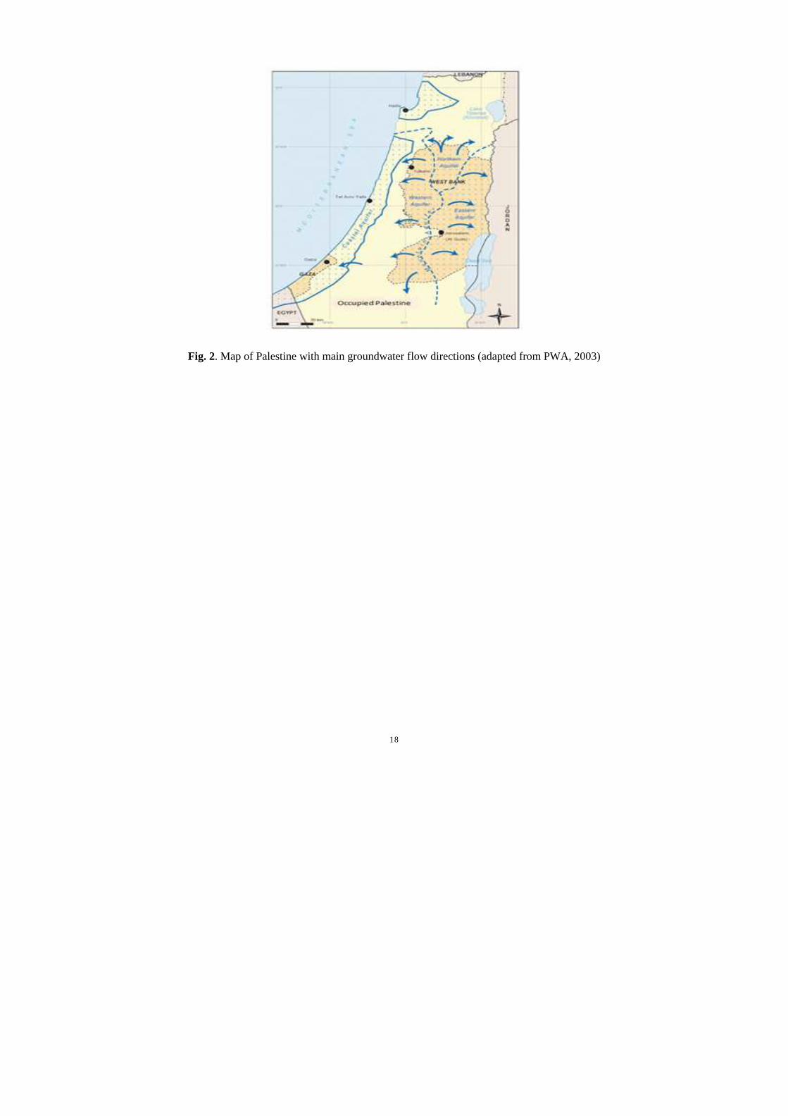
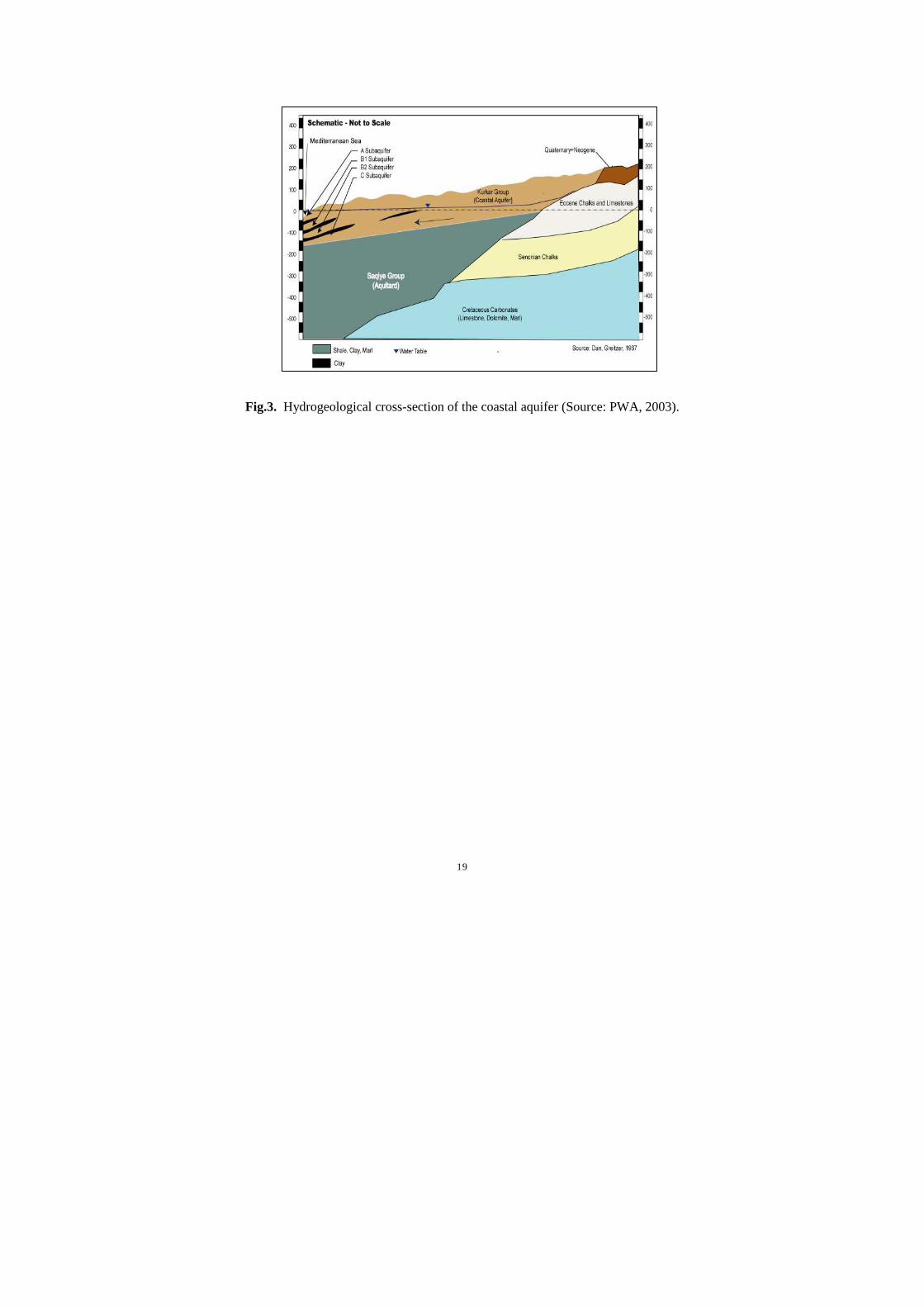
This coastal aquifer extends from the Gaza Strip in the south to Mount Carmel in the north along some 120 km of Mediterranean coastline (Fig.2). The width of the aquifer varies from 3-10 km in the north to about 20 km in the south. The total area of the coastal aquifer is about 2000 km2 with a small part of it beneath the Gaza Strip. The geology of the aquifer system in the area extends along the coastal plain of the Gaza Strip, which is of the Pliocene- Pleistocene geological age. The main aquifer consists of marine deposits of sandstone, calcareous siltstone and red loamy soils. The aquifer system is subdivided near the coast into 4 separate sub-aquifers, A, B1, B2, and C with largely unconfined and confined/unconfined multi-aquifer in the western part (PEPA, 1996) (see Fig.3). These sub-aquifers are separated by marine clay layers (aquitards), which have a thickness of about 20 meters and which extend by 2-5 km from the shoreline to inland. High rates of urbanization and increased municipal water demand, as well as extended agricultural activities, have increased the overall abstraction rate in the Gaza aquifer from 136 MCM (million cubic meters) in year 2000 to 174 MCM in 2010. This amount of water demand cannot be balanced anymore by natural replenishment by precipitation and have led to an overexploitation of the aquifer (Sirhan and Nigim, 2002). Due to the high groundwater pumping rates, the water levels across most of the coastal aquifer have dropped significantly and reached more than 12 m below mean sea level, inducing sea water intrusion and a subsequent deterioration of the freshwater quality as the chloride concentration has increased to more than 250 mg/l along the shoreline section of the aquifer as seawater intrusion and to the southeast section as a resulting of upconing. Beside that, some of the wells are already been closed due to the increase of chloride concentration (PWA, 2001).

3. ANN modeling approach

3.1 Data and selection of independent input variables for use in the ANN model

For a successful ANN model implementation, the availability of good data both in quantity and quality is necessary (Smith and Eli, 1995; Tokar and Johnson, 1999). Gathering such data is the first step in the development of an ANN model.

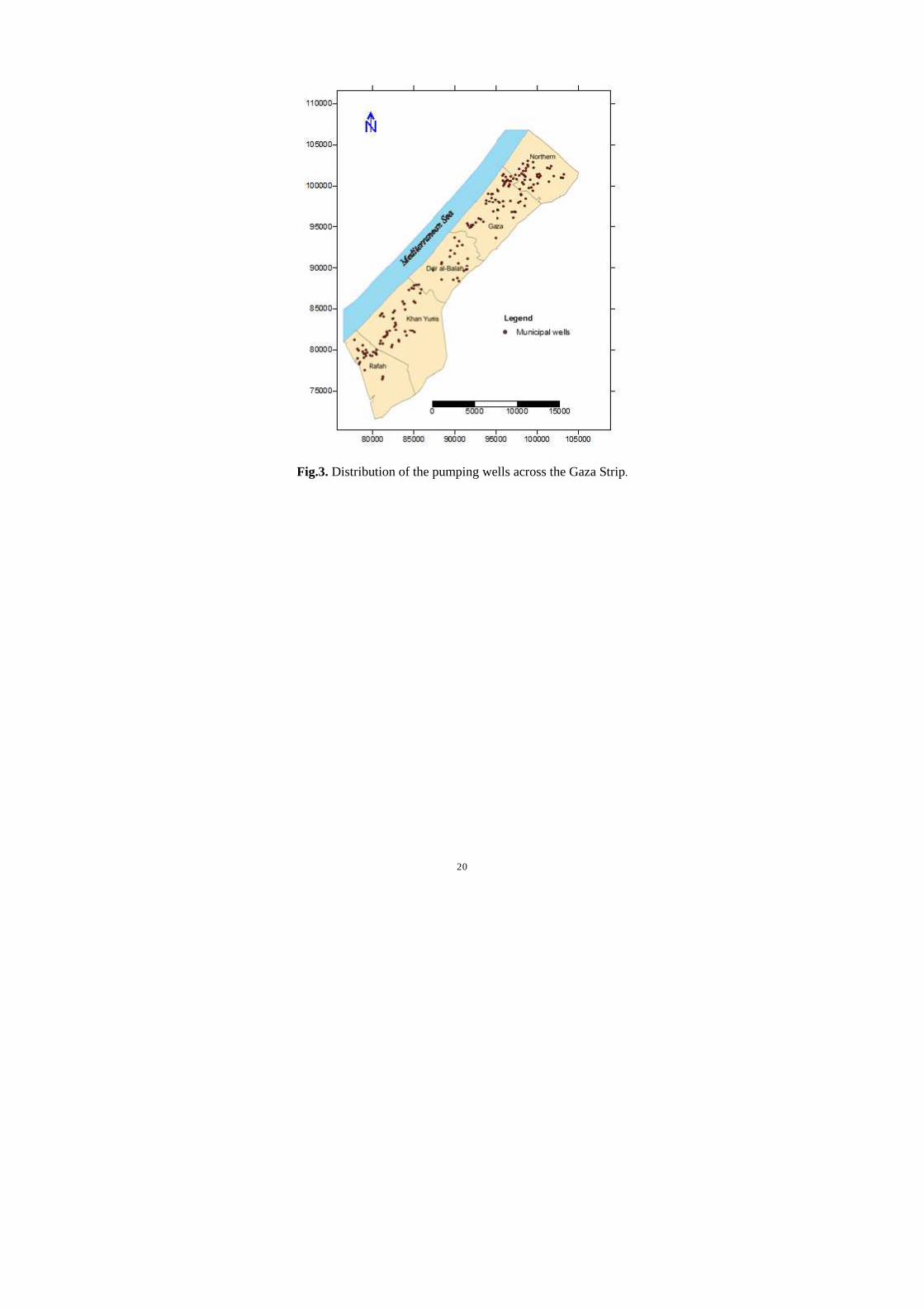
In the present study the data required has been obtained from the ministry of agriculture (MoA) in the Gaza strip and it consists of various sets of groundwater time series data, namely, yearly groundwater levels recorded at about 70, mostly municipal, wells all across the Gaza strip (see Fig. 4) over the 11-year time-span 2000-2010 and - to the extent that they are available - pumping rates. Since the raw data often contained missing records, or was afflicted by all kind of instrumental and human errors, it had to be cleaned and filtered properly, before it could be used in the ANN model training. Further details on the data and the analysis procedures employed are provided in Sirhan (2013).

5

The next step in the creation and design of a strong and accurate ANN model, in order to predict the output variables, consists in the selection of a set of significant input variables. From the results of Seyam and Mogheir (2011) who, as mentioned, set up an ANN model for the groundwater salinity in the area, one can get a first idea on possible significant independent input variables which will affect the dependent output variable (groundwater levels) in the present ANN model. These are, namely, the groundwater abstraction and the recharge from rainfall and surface water. A corroboration of this fact was obtained from correlation analyses of the (11 years x 70 wells = 770) long output column vector of the output (head) data with the two columns of the input matrix (abstraction and recharge), the results of which indicated, indeed, that these two variables serve well as the two main independent variables in the ANN-model. Nevertheless, an additional subset of other possible independent input variables was tested to serve as influential predictors in the ANN model. The latter were chosen based on knowledge about the physics and hydrogeology of the groundwater system under question, gained either from experience or from intermediate results of deterministic groundwater flow modeling in the study area. Here the MODFLOW groundwater model within the VISUAL MODFLOW environment has been used (see Sirhan, 2013 and Sirhan and Koch, 2013, for details). Eventually, in addition to the ground water extraction rate Q, the groundwater recharge from rainfall R, five more predictor input variables, namely, initial ground water level WLi, hydraulic conductivity K, distance of the abstraction wells from the shore line Dshore, depth of the well screen Dscreen and well-density Wdens are selected in the initial ANN model to predict the final output water levels WLf .

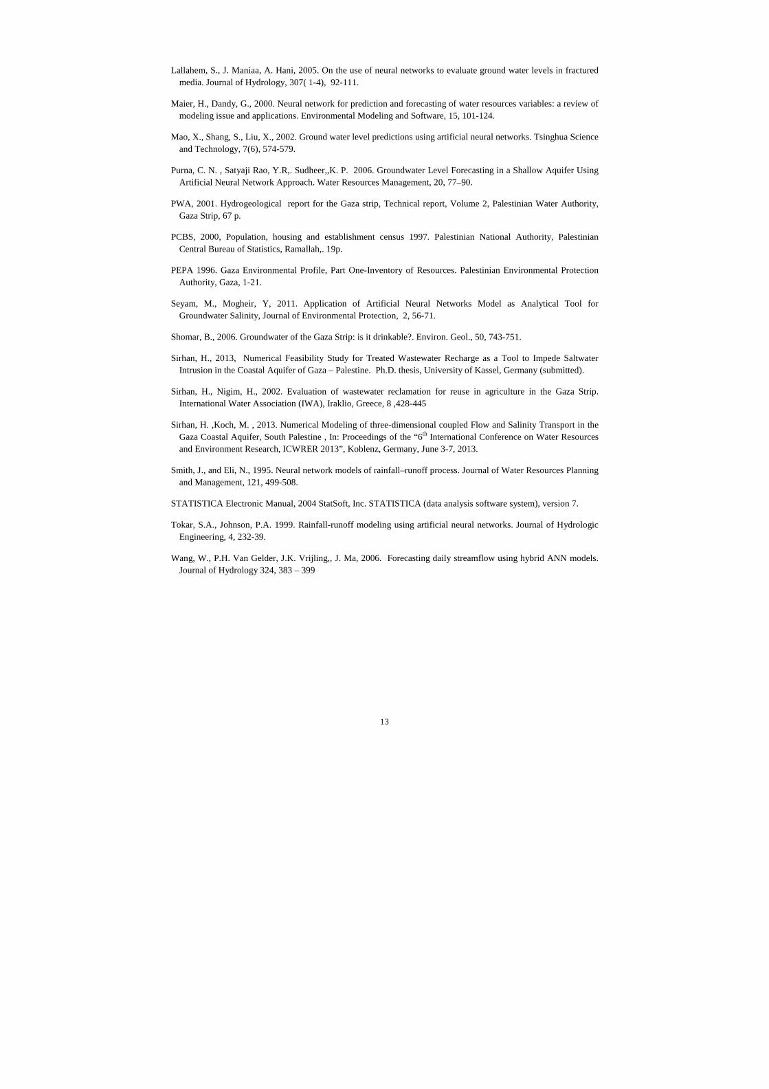
In Table 1 the basic descriptive statistical properties of these seven independent variables, namely, minimum, maximum, mean, median, standard deviation and coefficient of variation (= ratio of the standard-deviation to the mean of the data) are summarized.

3.2 General formulation of the ANN model

An ANN model describes a general functional relationship

Y = f (X) (1) ,

between some input (predictor) matrix X consisting of m independent variable vectors x1, x2, . . . , xm; and a dependent (predictand) output variable vector Y. Independent variables are those that are manipulated, whereas dependent variables are measured or registered. Goal of ANN modeling is then the quantification of the function f during the so-called training phase, so that new predictands can be forecast from other input variables in the subsequent prediction phase. As discussed in the previous section, the output variable vector Y in Eq. (1) consists here of the unknown final water levels WLf, which are supposed to depend on seven input parameter (column) vectors x1, x2, . . . , x7 of X, namely, WLi, Q, R, K, Dshore, Dscreen., and Wdens. Using these variables, Eq. (1) is then reads

WLf = f (WLi, Q, R, K, Dshore, Dscreen, Wdens) (2)

As will be shown during the optimization of the ANN model in the following sections, some of these seven independent variables turn out to be not significant for the prediction and can thus be omitted in the final ANN model.

6

3.3 Architecture and procedures to optimize the ANN model

The basic concept of an artificial neural network (ANN) is derived from an analogy with the biological nervous system of the human brain and how the latter processes information through its millions of neurons interconnected to each other by synapses. Borrowing this analogy, an ANN is a massively parallel system composed of many processing elements (neurons), where the synapses are actually variable weights, specifying the connections between individual neurons and which are adjusted, i.e. may be shut on or off during the training or learning phase of the ANN, similar to what is happening in the biological brain. However, here the analogy of a technical ANN with the real brain already comes to an end, as the architecture of the former is inevitably much simpler than that of the latter. Thus, the neurons in an ANN are usually set-up in consecutive layers, the so-called perceptrons, and information is going from the input nodes (neurons) in the first layer across one or several intermediate or hidden layers to the output nodes in the output layer (see Fig. 5). If this pure forward passing of information is not accompanied by extra cycles or loops within one layer, - which actually may happen in a biological brain - one speaks of a feed-forward neural network. It is the simplest form of an ANN and, for this reason, also the most commonly used in practice. Although the number of hidden layers between the input and output perceptrons could, in theory, be arbitrarily increased, to better mimic the functioning of the biological brain - in the case of which one also speaks of a multiple layer perceptron (MLP) network – the ensuing exponential increase of the neurons and, more so, of the synapses (the activation weights), makes such an approach totally impractical. Thus, most of the ANN used in practice are using only a few, or sometimes even none, hidden layers. For each application the most suitable architecture of the ANN is then determined by trial and error in the initial testing phase. In the training or learning phase of the ANN, using known information at the input and output neurons, the activation weights of the synapses connecting neurons in different layers are computed (see Fig. 5). This amounts to iteratively correcting initially estimated values of the weights, until the error between observed and predicted output is minimal. Mathematically this is equivalent to solving a multi-objective minimization or optimization problem and can be done, for example, by classical gradient methods, as they have been known for many decades in the field of general mathematical optimization (e.g. Gill et al. 1980). These methods are using the gradient of the error cost function to move step by step towards its minimum. In the ANN community this approach is also known as error back-projection, which means that errors occurring at a particular stage of the iteration process at the output layer are back-propagated consecutively through the various perceptrons of the ANN to compute corrections of the unknown activation weights (see Fig. 6). Similar to classic gradient optimization the derivative of the error cost function must be computed which means that the activation weights must derivable. For this reason the latter are set up in the form of a monotonously increasing activation function. In most ANN applications the so-called sigmoid function is used In spite of the widespread applications of the feed-forward MLP – ANN with error backprojection, as described above, the method may be prone to errors and instabilities for multidimensional problems, as it will often, likewise to the classical gradient method, find only a local, but not a global minimum of the error cost function. This means that the final optimal model will depend somehow on the initial conditions. To overcome partly this deficiency, radial

7

basis functions (RBF), which have some kind of a distance criterion built in with respect to a center, have been proposed, instead of the sigmoid functions to transfer information across the hidden layers. Usually only one hidden layer is used in such a RBF-ANN network and the non-linear RBF activation function- commonly taken to be a Gaussian is only applied to this layer, whereas the final transfer to the output layer is done in linear manner. The various procedure discussed above for setting up an ANN-model can be implemented either in a mathematical, such as the neural network toolbox of MATLAB, or a statistical computational environment, like neural network STATISTICA. The latter is used in this study STATISTICA is a comprehensive, integrated data analysis, graphics, and database management which is used in a wide range of engineering applications. Although the STATISTICA ANN module operates somewhat under a black box the user can select numerous tuning knobs to gear the program through the various steps of ANN model testing, learning, validation and prediction.

4. Results and discussion

4.1 Initial ANN

4.1.1 General characteristics and statistical performance

The initial ANN-model trials were formatted using all seven input variables (neurons) in Eq. (2). From the 770 observed water levels, half (=386) were selected randomly for the training of the model and the remaining half of the data was divided in two equal sets; one for validation and the other for testing (prediction).

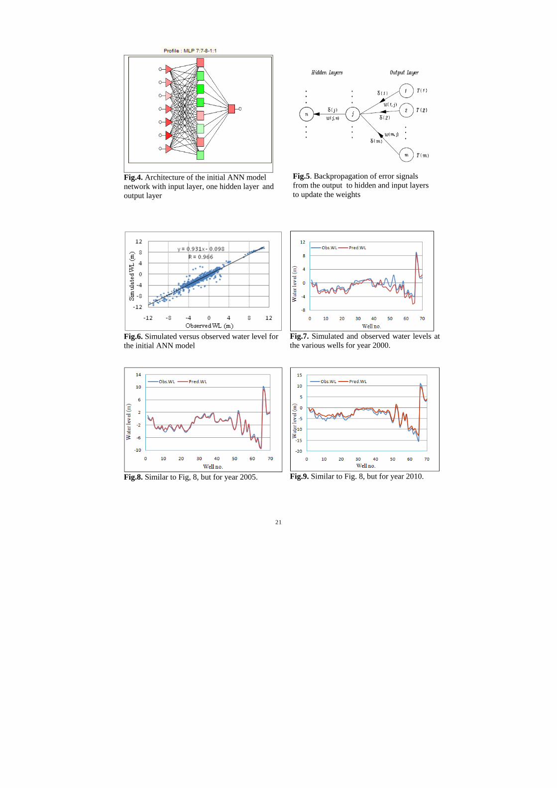
Practically, the training of the network consists of a forward propagation of the inputs and a backward propagation of the error (Fig.5). In the forward procedure, the effect of an applied activity pattern at the input layer is propagated through the network layer by layer. During network training, the data are processed through the ANN, and the connection weights are adjusted adaptively, until a minimum acceptable error is achieved between the predicted and the observed output Both, multilayer perceptron (MLP) and radial basis function (RBF) ANN models were examined. Many different models with different numbers of hidden layers and different activation functions were tested. To that avail an intelligent problem solver (IPS) to determine the model constraints which include optimization time, network type and the number of hidden units, and paying attention to the relationships among all input variables was developed. Surprisingly, and disproving somewhat the explanations of the previous section, the classical MLP network with a sigmoid activation function turned out to be better than a RBF- network. For this reason the latter ANN-option was not followed up further. The characteristics of the initial MLP-ANN model network are summarized in Table 2. This network has three perceptron layers, i.e. an input layer of 7 neurons, representing the variables in Eq. (2), a hidden layer with 8 neurons, and one output layer with one neuron (the final water level) (Fig.5). From the table one may note that the performance measure – defined as the ratio of the standard deviation of the predictions to that of the observations - for this network have low values for all three ANN-steps, i.e. training, validation and testing. Table 2 provides further characteristics of the selected ANN network. Thus, the notation BP100, CG20, CG40b in the last column indicates that one hundred passes of back-propagation, followed by twenty and forty epochs of conjugate gradient descents have been used for optimizing this model.

8

More details of the statistical results for this initial ANN-models are provided in Table 3, where various statistical indicators of the ANN-model simulations – some of which are discussed further in the following paragraphs - for the training, validation and test phases are listed individually.

In Fig. 7 the simulated water levels obtained for the optimal initial ANN model are plotted against the observed water levels. In addition, the fitted linear regression line is shown. As both the slope of this line and the correlation coefficient R (=0.966), the latter being equal to the square root of R2, the coefficient of determination, are close to one, the performance of this initial ANN model can be considered as very good. This R-value using all the data is to be compared to those obtained separately for the training, validation (selection), and testing phases. These are also listed in Table 3 and are R= 0.976, 0.948, and 0.958, respectively.

Predicted and observed water levels for the 70 well are shown for years 2000, 2005 and 2010 in Figs. 8, 9 and 10, respectively. One may notice a good agreement between the two for all these three years.

4.1.2 Sensitivity analysis

A sensitivity analysis can provide information on the usefulness and significance of individual input variables in the ANN model (STATISTICA 7 manual, 2004). The sensitivity of an independent input variable xi is normally measured by the ratio of the change of the model output ∆Y (see Eq. 1) to a change ∆xi of this input variable.

Another measure which is also sometimes used in statistical inference, namely, in stepwise regression, is to compare the mean squared error (MSE) between observed and predicted datum for the two cases when a particular variable xi is included or not included in the model. In ANN-applications it has been more common to use the mean absolute error MAE instead, defined as

MAE = 1/n*∑ |Yiobs - Yi

sim | (3)

where Yiobs and Yi

sim are the observed and ANN-simulated datum, respectively, and n is the number of observations. The MAEs of the initial ANN- model obtained for the training, validation and test phases have also been listed in Table 3.

The sensitivity of the ANN model to a particular variable is then computed (e.g. Coppola et al., 2003; Feng et al., 2008) based on the ratio of the MAE when a particular variable is not included in the model to that when it is included, i.e.

(4)

Under normal situations the MAE in the nominator of Eq. (4) is larger than that in the denominator, since the omission of a particular variable will usually deteriorate the performance of the ANN-model, i.e. the MAE will be increased. This means also that the more important an input variable is in the ANN-model, the higher than one is the ratio in Eq. (4). Thus, the size of

9

the ratio allows a ranking of the importance of each variable, relative to all other variables. Meanwhile, a ratio of less than 1 will also indicate that the elimination of that input variable actually increases the ANN-model accuracy.

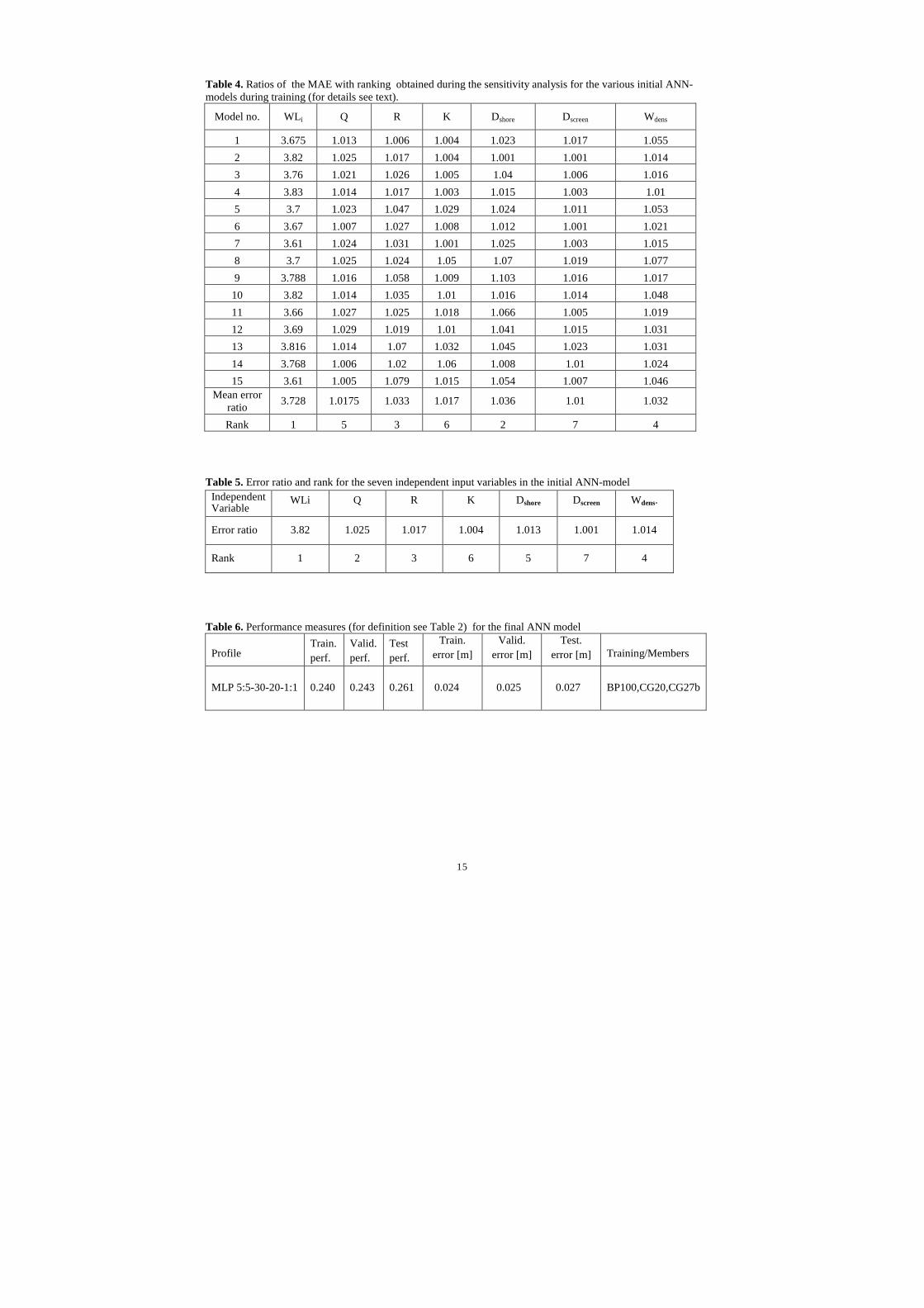
In the practical sensitivity study, a total of fifteen ANN models were analyzed, whereby a single input variable out of the originally seven in the initial model (see Eq. 2) was excluded one by one, and the corresponding error ratio (4) computed. These are listed in Table 4 for the training phases for the 15 ANN-models tested, together with the mean error ratio. From the ranking of the latter, the relative importance of the seven different input parameters is inferred. The last row of Table 4 then indicates, that the two independent variables, depth to well-screen Dscreen and hydraulic conductivity K, are the least-influential variables affecting the final groundwater levels WLf, as these have the smallest error ratios. An additional correlation analysis showed furthermore that these these two variables are only lowly correlated with the observed water levels WLf which provides additional evidence that they can be safely ignored in the build-up of an optimal ANN model. Consequently, a new training of the network has been carried out in the following section where only the retained, most important five input variables are incorporated in the model. To conclude this section, the MAE–ratio’s of the overall initial ANN- model, i.e. using all data, are listed in Table 5, together with the corresponding ranks of the influences of the 7 input variables. This table corroborates the results of Table 4 with regard to the selection of the 5 most influential input variables in the set-up of the final ANN model.

4.2 Final ANN model

4.2.1 General characteristics and statistical performance

Based on the sensitivity ranking of the seven input parameters used in the initial ANN model (see Table 5), the final neural network models were formatted employing only the five input variables (neurons) WLi, Q, R, Dshore and Wdens.

Similar to the initial ANN- model, in this final ANN model test series the 770 observed output data (neurons) were divided randomly into three groups; a first one with 386 data cases for training, a second one with 192 data for validation, and a third one with the remaining 192 cases for testing (prediction). Also both MLP- and RBF–models were executed again and compared to each other.

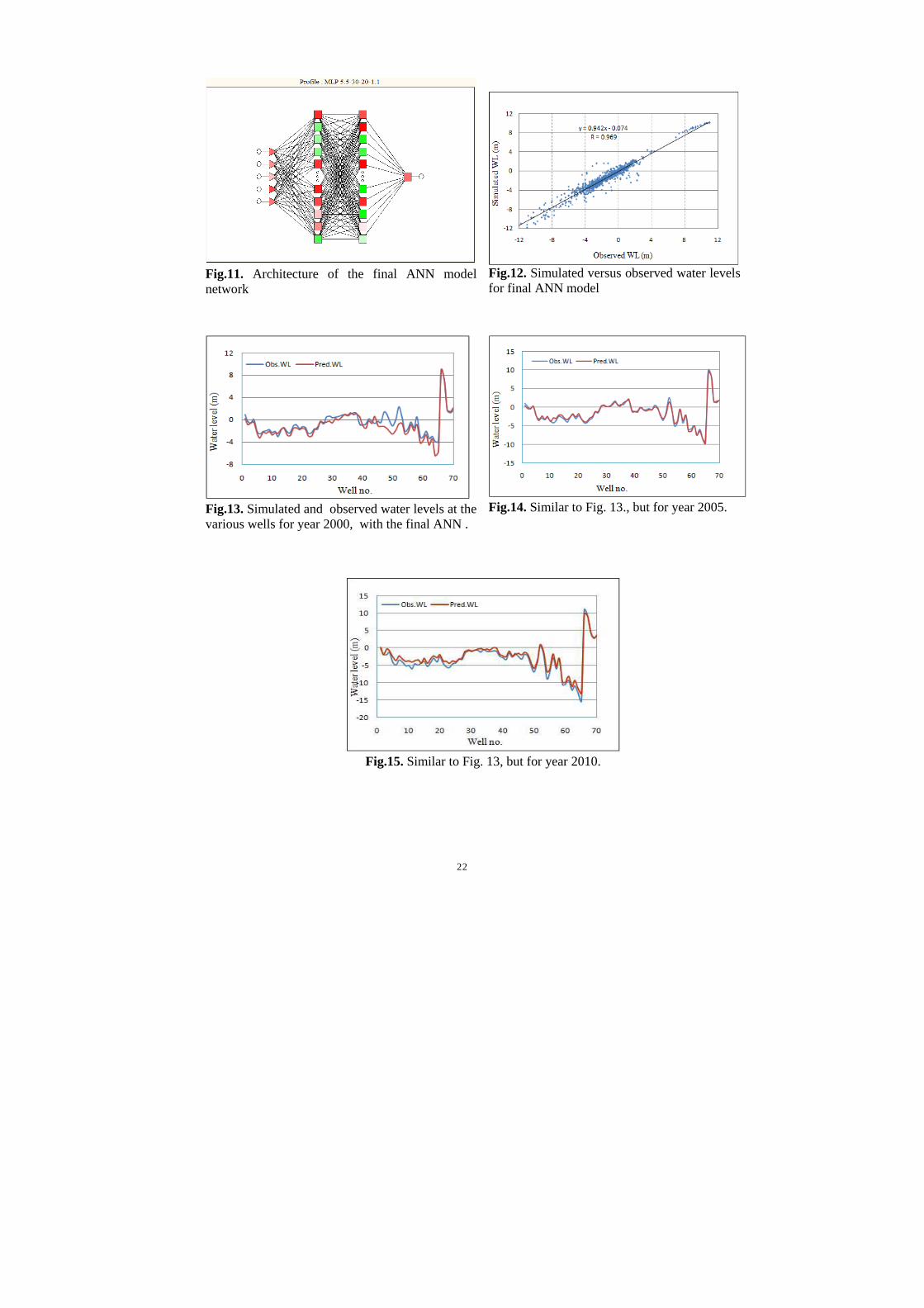
The best network performance was attained with a four-MLP network, i.e. with two hidden layers (perceptrons) between the input and output layer, and using a sigmoid activation function in between these layers. More specifically, the input layer has 5 neurons, representing the specified input variables, a first hidden layer with 30 neurons, a second hidden layer with 20 neurons and the final output layer with one neuron, representing the output groundwater levels. Fig. 11 shows the architecture of this final ANN model.

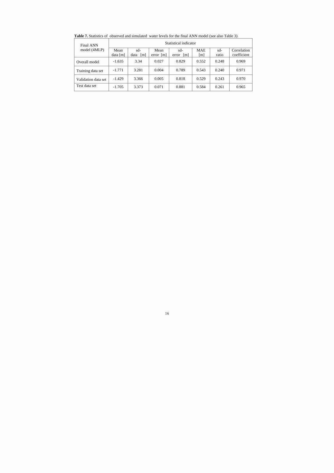
The performance characteristics of this final ANN- model are summarized in Table 6 and may be compared with those of the initial ANN- model listed in Table 3. From these numbers one can deduce that the final ANN-model works better than the initial one for the validation and testing phases.

10

Fig 12. indicates that this final ANN fits the observed output very well, with a correlation coefficient R=0.969 for the regression line between simulated and observed water levels. The corresponding R-values for the training, validation and test set are 0.971, 0.970 and 0.965, respectively (Table 6). As these R-values are more or less identical to the ones of the initial ANN- model (Table 3), the advantage of this final ANN-model may not become immediately clear. However, as this final model has been obtained with a smaller number of input parameters than the initial one (5 against 7, respectively), it abides better by the rule of parsimony, which is an important selection criterion in statistical estimation.

The groundwater levels simulated with this final ANN model are shown for the years 2000, 2005 and 2010, in Figs. 13, 15 and 15, respectively. Similar to the initial ANN-model (Figs. 8, 9 and 10) a very good agreement of the modeled and the observed water levels is also noticed for this final ANN-model. .

4.2.2 Response graphs and response surfaces

Eq. (2) may be viewed upon as an m-dimensional hypersurface of the response variable final water level WLf, as a function of the m independent input variables of the ANN-model. For an approximate visualization of such a hypersurface either one-dimensional response graphs or two-dimensional response surfaces may be used

Response graphs represent a one-dimensional slices through the hypersurface along the direction of one independent variables with the remaining ones hold constant..

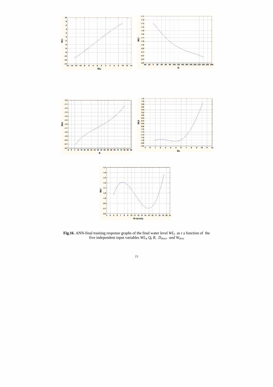
Fig.16 shows the response graphs of the final water levels WLf for each of the 5 input variables of the final ANN model, namely, WLi, Q,,R, Dshore, and Wdens. From the visual inspection of these response graphs, the dependency of the output variable on a particular input variable can be clearly identified. For example, the first three panels of Fig 16 show that WLf increases monotonously with the initial water levels WLi, and the groundwater recharge R, but decreases with the pumping (abstraction) rate Q. In contrast, the variations of WLf as a function of the distance of the well to the shore Dshore and of the well-density Wdens are more complicated, since the corresponding graphs exhibit some oscillatory, or unstable behavior.

Response surfaces can explain relationships between pairs of two independent input variables and of the output dependent variable. Because the number of combination pairs with five input variables is too high, to be all shown, in Fig. 17 only pairs with the pumping rate Q as one partner are plotted.

Based on the visual inspection of these response surfaces, several statements can be made. Thus it can be seen that the final water levels WLf, are particularly sensitive to the initial water levels WLi (Fig.17a). and, depending on the pumping rate Q, also on Dshore (Fig.17c). Fig. 17d indicates also that for high pumping rates Q, the well-density Wdens has also a strong effect on the final water levels.

5. Conclusions

The the ongoing depletion of the coastal aquifer in the Gaza strip due to overexploitations has led to a decline of groundwater levels, excessive reductions in yields, and many groundwater wells even going dry. Some of these wells had already to be shut down, due to an increase of

11

the groundwater salinity above the WHO- 250 mg/L drinking standard limit, i.e. a significant deterioration of groundwater has occurred all across the Gaza strip The ANN technique has been applied as a new approach and an attractive tool to study and predict groundwater levels without applying physically based hydrologic parameters. This approach may improve the understanding of complex groundwater system and is able to show the effects of hydrologic, meteorological and anthropical impacts on the groundwater conditions. The results presented in this study are based on the ANN technique through a feed forward neural network, where the network is trained using forward propagation of the inputs and backward propagation of the error, to update the unknown activation weights between the neurons of the different layers. Thus, the neural network model acts as a black box which passes information from input neurons through some internal (hidden) layers with neurons network to the output neurons. As this information process is not based on the real physics of the dynamical system, an ANN model will not provide further insight neither, which can be considered as a disadvantage of this methodology.

The optimal ANN-model for predicting groundwater levels in the Gaza coastal aquifer is developed in two major steps. In the first step an initial ANN-model is set up as a - after numerous trial and error tests – 3-layer MLP network and using the seven variables, initial groundwater level, groundwater extraction rate, recharge from rainfall, hydraulic conductivity, distance of a well from the shoreline, depth to the well screen and the well density across the area, as input neurons. This initial ANN model results in a very good agreement between simulated and observed groundwater levels with a correlation coefficient of R=0.966 In the subsequent sensitivity analysis the influential model input parameters are analyzed by computing the significance of individual variables in the ANN model. The results of this sensitivity analysis, using the ranks of the parameter influences indicate that the two independent variables, depth to well screen and hydraulic conductivity, are the least important variables for predicting the groundwater levels and can thus be ignored in the ANN model. In the second step the final ANN-model is set up retaining only the five most influential input variables. After numerous trials the best final ANN model is found to be a four MLP-(5:5:30:20:1) network with two hidden layers between input and output layer. This final ANN model is trained, validated and tested successfully, and results in an overall correlation coefficient of R=0.969 between simulated and observed groundwater levels Finally both response graphs and response surfaces are used to get some more physical insight into the aquifer system’s behavior by studying the relationships between independent and dependent variables. Thus monotonous increases of the final water levels with the initial water levels and with the groundwater recharge R, but decreases with the pumping (abstraction) rate are observed, whereas the dependencies of the former on the distance of the wells to the shore and on the well density are not so clear..

12

Acknowledgments

Thanks are extended to the people in the Gaza strip for their assistance in field investigations, and for providing some necessary information. Helpful discussions with Dr. Khalid Qahaman are also gratefully acknowledged.

References

Anderson. M. , W. Woessner, 1991. Applied groundwater modeling simulation of flow and advective transport. Academic Press, San Diego, CA, 381p.

Affandi, A., K.. Watanabe, 2007. Daily groundwater level fluctuation forecasting using soft computing technique. Nature and Science, 5(2), 1-10.

Chuanpongpanich, S., P. Arlai, M. Koch, K. Tanaka, T. Tingsanchali, 2012, Inflow Prediction for the Upstream Boundary of the Chao Phraya River Integrated River Model using an Artificial Neural Network, Proceedings of the 10th International Conference on Hydroscience and Engineering, Orlando, Florida, November 4–7, 2012.

Coppola, E., F. Szidarovszky, M. Poulton, E. Charles, 2003. Artificial neural network approach for predicting transient water levels in a multilayered ground water system under variable state, pumping, and climate conditions., Journal of Hydrological Engineering, 8(6), 348–359.

Coppola, E., Rana, A., Poulton, M., Szidarovszky, F., Uhl, V., 2005. A neural network model for predicting water table elevations. Ground Water, 43( 2), 231-241.

Coppola, E., F. Szidarovszky, D. Davis, 2007. Multiobjective analysis of a public wellfield using artificial neural networks. Ground Water, 45 (1) , 53–61.

Coulibaly, P., F. Anctil, B. Bobee. 1999. Hydrological forecasting using artificial neural networks: the state of the art (in French). Canada Journal Civil Engineering,, 26 (3), 293–304

Coulibaly, P., Anctil, F., Aravena, R., Bobee, B., 2001. Artificial neural network modeling of water table depth fluctuation. Water Resources Research, 37(4), 885-896.

Daliakopoulos, I., Coulibaly, P., Tsanis, I., 2005. Ground water level forecasting using artificial neural networks. Journal of Hydrology, 309( 1-4), 229-240.

De Vos, N., Rientjes, T., 2005. Constraints of artificial neural networks for rainfall-runoff modelling: trade-offs in hydrological state representation and model evaluation. Hydrology and Earth System Sciences, 9, 111-126.

Dibike, Y.B., D. Solomatine, M.B. Abbott, 1999. On the encapsulation of numerical-hydraulic models in artificial neural networks. Journal of Hydraulic Research, 37, 147-161

Feng, S., Kang, S., Huo, Z., Chen, S., Mao, X., 2008. Neural Networks to Simulate Regional Ground Water Levels Affected by Human Activities. Ground Water, 46(1), 80-90.

Gill, P.E., W. Murray, M. H. Wright, 1981, Practical Optimization, Academic Press, Orlando, Fl, 401p

Govindaraju,, R., 2000. Artificial Neural Network in Hydrology. Journal. Hydrologic Engineering, 5(2), 124 - 137..

Kresic, N., 1996. Quantitative solutions in hydrogeology and groundwater modelling, Lewis, Atlanta, GE., 307p.

Jalalkamali, A.,. N. Jalalkamali,,,2011. Groundwater modeling using hybrid of artificial neural network with genetic algorithm. African Journal of Agricultural Research. 6(26), 5775-5784.

13

Lallahem, S., J. Maniaa, A. Hani, 2005. On the use of neural networks to evaluate ground water levels in fractured media. Journal of Hydrology, 307( 1-4), 92-111.

Maier, H., Dandy, G., 2000. Neural network for prediction and forecasting of water resources variables: a review of modeling issue and applications. Environmental Modeling and Software, 15, 101-124.

Mao, X., Shang, S., Liu, X., 2002. Ground water level predictions using artificial neural networks. Tsinghua Science and Technology, 7(6), 574-579.

Purna, C. N. , Satyaji Rao, Y.R,. Sudheer,,K. P. 2006. Groundwater Level Forecasting in a Shallow Aquifer Using Artificial Neural Network Approach. Water Resources Management, 20, 77–90.

PWA, 2001. Hydrogeological report for the Gaza strip, Technical report, Volume 2, Palestinian Water Authority, Gaza Strip, 67 p.

PCBS, 2000, Population, housing and establishment census 1997. Palestinian National Authority, Palestinian Central Bureau of Statistics, Ramallah,. 19p.

PEPA 1996. Gaza Environmental Profile, Part One-Inventory of Resources. Palestinian Environmental Protection Authority, Gaza, 1-21.

Seyam, M., Mogheir, Y, 2011. Application of Artificial Neural Networks Model as Analytical Tool for Groundwater Salinity, Journal of Environmental Protection, 2, 56-71.

Shomar, B., 2006. Groundwater of the Gaza Strip: is it drinkable?. Environ. Geol., 50, 743-751.

Sirhan, H., 2013, Numerical Feasibility Study for Treated Wastewater Recharge as a Tool to Impede Saltwater Intrusion in the Coastal Aquifer of Gaza – Palestine. Ph.D. thesis, University of Kassel, Germany (submitted).

Sirhan, H., Nigim, H., 2002. Evaluation of wastewater reclamation for reuse in agriculture in the Gaza Strip. International Water Association (IWA), Iraklio, Greece, 8 ,428-445

Sirhan, H. ,Koch, M. , 2013. Numerical Modeling of three-dimensional coupled Flow and Salinity Transport in the Gaza Coastal Aquifer, South Palestine , In: Proceedings of the “6th International Conference on Water Resources and Environment Research, ICWRER 2013”, Koblenz, Germany, June 3-7, 2013.

Smith, J., and Eli, N., 1995. Neural network models of rainfall–runoff process. Journal of Water Resources Planning and Management, 121, 499-508.

STATISTICA Electronic Manual, 2004 StatSoft, Inc. STATISTICA (data analysis software system), version 7.

Tokar, S.A., Johnson, P.A. 1999. Rainfall-runoff modeling using artificial neural networks. Journal of Hydrologic Engineering, 4, 232-39.

Wang, W., P.H. Van Gelder, J.K. Vrijling,, J. Ma, 2006. Forecasting daily streamflow using hybrid ANN models. Journal of Hydrology 324, 383 – 399

14

Tables

Table 1. Descriptive statistics for the independent observed variables used in the ANN-model

Variable Unit Min. Max. Mean Median Std. Dev.

Coef. Variat.1

Initial water level WLi M -12.8 10.73 -1.45 -1.38 3.11 -2.14

Abstraction rate Q M3/hr 0 240.9 75.53 64.64 61.1 0.81

Recharge rate R mm/m2/month 6.57 80.15 26.93 21.15 15.98 0.59

Hydraulic conductivity K m/d 15 40 31.21 30 8.97 0.29

Distance from shore Dshore Km 0.8 10.19 3.63 3.1 2.11 0.58

Distance to well screen screen M 8.95 122.3 64.54 65.6 30.13 0.47

Well density Wdens No./km2 4.9 19.32 10.5 9.96 5.19 0.49

1defined as the ratio of the standard deviation to the mean

Table 2. Performance measures1 for the initial ANN model

Profile Train. perf.

Valid. perf.

Test perf.

Train. error [m]

Valid. error [m]

Test error [m]

Training/Members

MLP 7:7-8-1:1 0.217 0.318 0.286 0.023 0.031 0.026 BP100,CG20,CG40b

1defined as the ratio of the standard deviation of the ANN-predictions to that of the observations

Table 3. Statistics of observed and simulated water levels for the initial ANN model

Statistical indicator Initial ANN model (3-MLP) Mean

data [m] sd- data [m]

Mean error [m]

sd- error [m]

MAE1 [m]

sd- ratio2

Correlation coefficient

Overall model -1.671 3.329 0.016 0.859 0.572 0.258 0.966

Training data set -1.666 3.525 -0.017 0.765 0.543 0.217 0.976

Validation data set -1.620 3.237 0.055 1.030 0.635 0.318 0.948

Test data set -1.732 2.980 0.047 0.854 0.571 0.286 0.958

1defined in Eq. (3) 2defined as the ratio of the standard error of the ANN-model (sd error) to that of the data (sd data) and corresponds to the performance measure in Table 2.

15

Table 4. Ratios of the MAE with ranking obtained during the sensitivity analysis for the various initial ANN- models during training (for details see text).

Model no. WLi Q R K Dshore Dscreen Wdens

1 3.675 1.013 1.006 1.004 1.023 1.017 1.055

2 3.82 1.025 1.017 1.004 1.001 1.001 1.014

3 3.76 1.021 1.026 1.005 1.04 1.006 1.016

4 3.83 1.014 1.017 1.003 1.015 1.003 1.01

5 3.7 1.023 1.047 1.029 1.024 1.011 1.053

6 3.67 1.007 1.027 1.008 1.012 1.001 1.021

7 3.61 1.024 1.031 1.001 1.025 1.003 1.015

8 3.7 1.025 1.024 1.05 1.07 1.019 1.077

9 3.788 1.016 1.058 1.009 1.103 1.016 1.017

10 3.82 1.014 1.035 1.01 1.016 1.014 1.048

11 3.66 1.027 1.025 1.018 1.066 1.005 1.019

12 3.69 1.029 1.019 1.01 1.041 1.015 1.031

13 3.816 1.014 1.07 1.032 1.045 1.023 1.031

14 3.768 1.006 1.02 1.06 1.008 1.01 1.024

15 3.61 1.005 1.079 1.015 1.054 1.007 1.046 Mean error

ratio 3.728 1.0175 1.033 1.017 1.036 1.01 1.032

Rank 1 5 3 6 2 7 4 Table 5. Error ratio and rank for the seven independent input variables in the initial ANN-model

Independent Variable

WLi Q R K Dshore Dscreen Wdens.

Error ratio 3.82 1.025 1.017 1.004 1.013 1.001 1.014

Rank 1 2 3 6 5 7 4

Table 6. Performance measures (for definition see Table 2) for the final ANN model

Profile Train. perf.

Valid. perf.

Test perf.

Train. error [m]

Valid. error [m]

Test. error [m] Training/Members

MLP 5:5-30-20-1:1

0.240 0.243 0.261 0.024 0.025 0.027 BP100,CG20,CG27b

16

Table 7. Statistics of observed and simulated water levels for the final ANN model (see also Table 3)

Statistical indicator Final ANN model (4MLP) Mean

data [m] sd-

data [m] Mean

error [m] sd-

error [m] MAE [m]

sd- ratio

Correlation coefficient

Overall model -1.635 3.34 0.027 0.829 0.552 0.248 0.969

Training data set -1.771 3.281 0.004 0.789 0.543 0.240 0.971

Validation data set -1.429 3.366 0.005 0.818 0.529 0.243 0.970

Test data set -1.705 3.373 0.071 0.881 0.584 0.261 0.965

17

Figures

Fig.1. Location of the Gaza strip study area.

18

Fig. 2. Map of Palestine with main groundwater flow directions (adapted from PWA, 2003)

19

Fig.3. Hydrogeological cross-section of the coastal aquifer (Source: PWA, 2003).

20

Fig.3. Distribution of the pumping wells across the Gaza Strip.

21

Fig.4. Architecture of the initial ANN model network with input layer, one hidden layer and output layer

Fig.5. Backpropagation of error signals from the output to hidden and input layers to update the weights

Fig.6. Simulated versus observed water level for the initial ANN model

Fig.7. Simulated and observed water levels at the various wells for year 2000.

Fig.8. Similar to Fig, 8, but for year 2005.

Fig.9. Similar to Fig. 8, but for year 2010.

22

Fig.11. Architecture of the final ANN model network

Fig.12. Simulated versus observed water levels for final ANN model

Fig.13. Simulated and observed water levels at the various wells for year 2000, with the final ANN .

Fig.14. Similar to Fig. 13., but for year 2005.

Fig.15. Similar to Fig. 13, but for year 2010.

23

Fig.16. ANN-final training response graphs of the final water level WLf as r a function of the five independent input variables WLi, Q, R, Dshore and Wdens

24

(a)

(b)

(c)

(d)

Fig.17. ANN-final training response surfaces WLf for various pairs of the input variables: (a) WLi & Q, (b) R & Q, (c) Dshore & Q, and (d) Wdens & Q