Prediction of Dam Deformation Using Kalman Filter Technique · PDF file · 2014-07-03Prediction of Dam Deformation Using Kalman filter Technique, ... of time and varying loads

Prediction of Dam Deformation Using Kalman filter Technique, (6848) Raphael Ehigiator - Irughe, Jacob Ehiorobo and Mabel Ehigiator (Nigeria) FIG Congress 2014 Engaging the Challenges – Enhancing the Relevance Kuala Lumpur, Malaysia 16-21 June 2014

1/14 Predicti

Prediction of Dam Deformation Using Kalman Filter Technique

Raphael EHIGIATOR-IRUGHE, Jacob Odeh EHIOROBO and Mabel O. EHIGIATOR, NIGERIA.

Key Words: Kalman Filter, Deformation Monitoring, Kinematic Model, GPS, State Vector

SUMMARY

In Dam Deformation Monitoring repeated observation are carried out to determine either relative or absolute Deformation of the structure. In some cases factors beyond the control of the observer or instrument may make it impossible to obtain reliable results from continuous measurement. In that case other methods of estimation or prediction of the deformation at some future data may be adopted.

Time dependent monitoring of the structures can be carried out using Kinematic and dynamic models in the analysis of the deformation. Such Time and position dependent measurements can be processed using the Kalman Filter equation. The Kalman filter equation estimates measurement parameters using time update and measurement update equations.

The time update equation predicts the results for the next epoch measurement while the measurement update equation serves as a corrector for the next step of the deformation measurement epoch. In this study Kalman filtering technique was used in predicting current estimates of Dam deformation using two previous GPS measurements carried out in 2007 and 2008 respectively. The Kalman filter equation was then used to compute the velocity and acceleration of the Dam object.

From these results coordinates changes were estimated for 2009, 2010, 2011 and 2012 respectively. Analysis of the results for 2008 show a strong correlation between the measurement updates and the predicted coordinates. It can therefore be concluded that the Kalman filtering equation can be used to fill in gaps in deformation measurement where continuous monitoring may not be possible within some epoch.


2/14 Predicti

Prediction of Dam Deformation Using Kalman Filter Technique

Raphael EHIGIATOR-IRUGHE, Jacob Odeh EHIOROBO and Mabel O. EHIGIATOR, NIGERIA.

1. INTRODUCTION

In analyzing deformation of structures such as Dams various deformation models have been developed. These models consist of static, Kinematic and dynamic models (Acar et al 2000 Lihua 2008).In dynamic deformation models, the deformation as the output signals are a function of time and varying loads.

In the static deformation model, the deformation is function of varying loads only. In Kinematic model, the deformation is described as a function of time. When GPS is used in the measurement of the movement of the Dam from surface measurement, there are no acting forces considered in term of a Kinematic model. The Kinematic/ dynamic parameters of deformation in a structure such as a Dam can be estimated by use of the Kalma Filter equation. The Kalman filter was designed to estimate the linear dynamic system (Kalma 1960, Kalman and Bucy 1961, cankut and sahin 2000). Welch and Bishop (2006) defined the Kalman filter as a set of mathematical equations that provides an efficient computational means to estimate the state of a process in a way that minimizes the mean of the square error.

Maybeck (1979) described the Kalma filter as simply an optimal recursive data processing algorithm that blend all available information including measurement outputs, prior knowledge about the system and measuring sensors to estimate the state variables in such a manner that the error is statistically minimized.

Kaplan (1993) on the other hand defined the Kalma filter as a recursive algorithm that provides optimum estimates of user position, velocity and Time based on noise statistics and current measurements. The filter contains a dynamic model of the GPS receiver platform motion and output a set of user receiver Position, Velocity and Time (PVT) state estimates as well as associated error variances.

The filter estimates a process state at some time and then obtain a feedback in the form of noisy measurements. Thus, the equation for the Kalman filter consist of time update equation that projects forward ( in time) the current state and error covariances estimates to get a priori estimate for the next time step and the measurement update equation which incorporates new measurements into the priori estimate to get an improved posteriori estimate.


3/14 Predicti

The Kalman filter is very convenient in estimating the state vector of a deformation object (Ince and sahin 2000, Grewal and Andrew 1993). The elements of the state vector in the Kalman filter include position (X Y Z) in the object or deformable body and variation of the position.

The Kalman filter supports estimation of past, present and future states of a dynamic system. Used without stochastic parameters, the kalman filter is regarded as a recursive solution of the Gauss original least-squares problems. In the filtering however, the number or observation can be less than the number of unknowns.

2. DESCRIPTION OF STUDY AREA

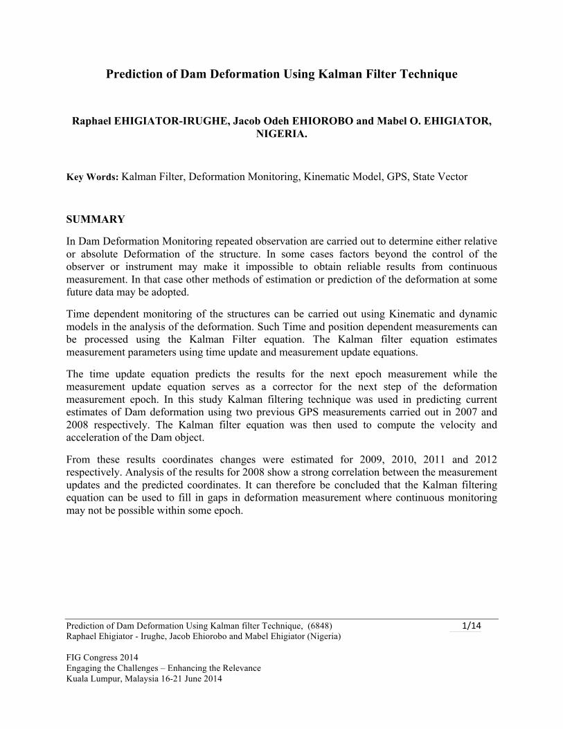
The Ikpoba River Dam is located in Benin City, the capital of Edo State of Nigeria The Dam together with its head works is located about 6km from the city centre (see fig 1)

Fig 1: Location Map of Ikpoba Dam in Benin City, Nigeria.

The Ikpoba Dam water supply scheme was designed to supply 160,000,000 litres of water per day at ultimate capacity. This account for about 60% of the water supply requirement for Benin City with a population of about 1.5 million.


4/14 Predicti

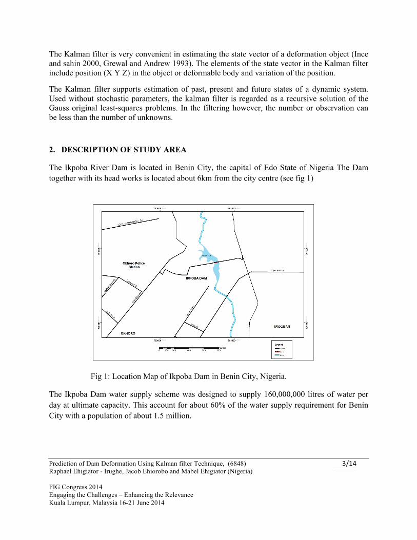
The network for Deformation monitoring consist of eleven control points both around the upstream and downstream are of the dam and Nine monitoring points established on the Dam crest Fig 2.

Fig 2: Layout of Control of Reference Point within the Dam area.

3. METHODOLOGY 3.1 DATA COLLECTION The data collection of the first GPS campaign took place during the period 11th and 12th of August 2007 and the second campaign on the 17th and 18th of August 2008. T

Four units of Leica 500 GPS systems and their corresponding accessories including a12 volt battery were deployed.

The GPS data were collected in static mode and post processed using Leica Ski-PRO software.

3.2 KINEMATIC DEFORMATION MODEL: THE KALMAN FILTER

The kalman Filter was designed to be a recursive solution to the discrete data linear filtering problem (Kalman 1960, Welch and Bishop 2006). When GPS is used in the determination of Deformation in a dam from surface measurements, there are no acting forces available and the deformation can be considered in terms of a Kinematic model.


5/14 Predicti

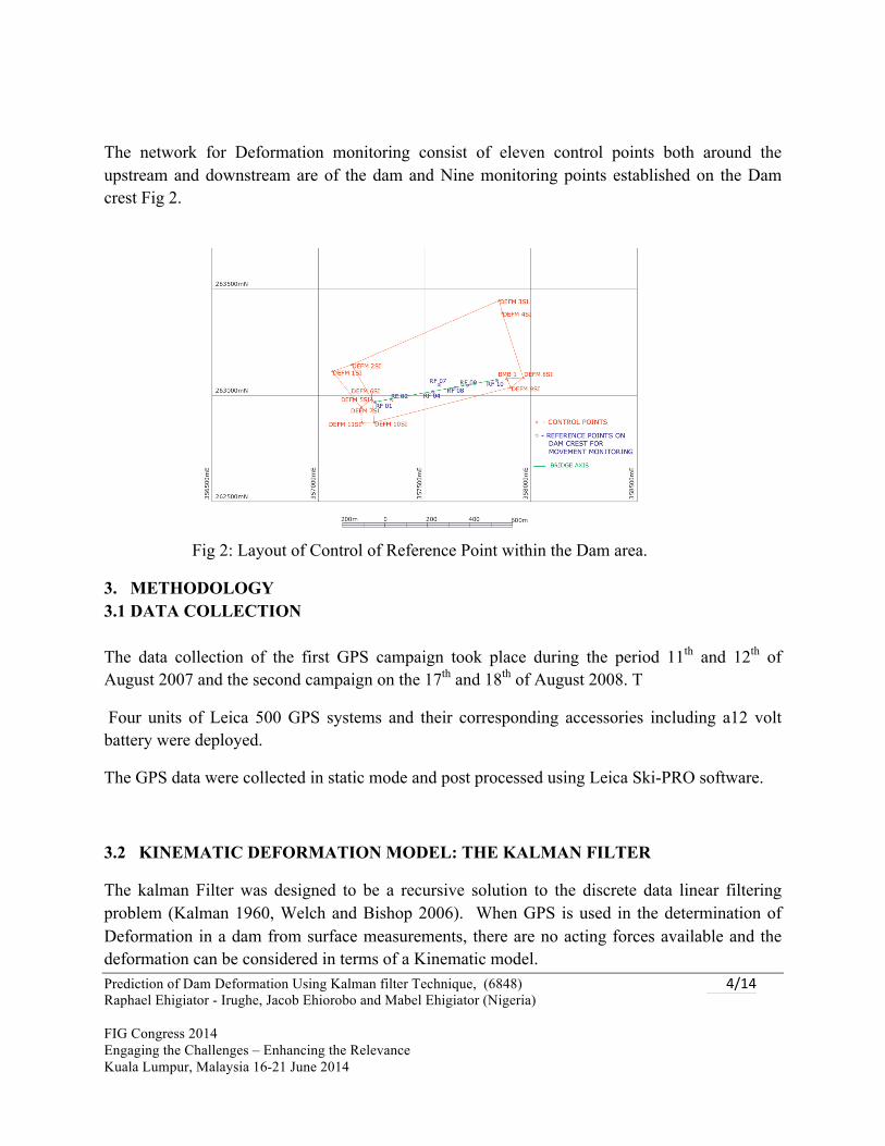
Kinematic deformation model determines displacements, velocity and acceleration and is time dependent. A time dependent 3-D Kinematic model that contain position, velocity and acceleration can be expressed using the equation (Acar et al 2000)

Xj

k + 1 = Xj(k) + (tk + 1 - tk) Vxj + ½ (tk + 1 - tk )2 axj

Yj

k + 1 = Yj(k) + (tk + 1 - tk) Vyj + ½ (tk + 1 - tk )2 ayj -----------------(1)

Z jk + 1 = Zj

(k) + (tk + 1 - tk) Vzj + ½ (tk + 1 - tk )2 azj

In eq (1), Xj

k + 1, Yjk + 1, Z j

k + 1 - Coordinates of points j at time (tk + 1) period Xj

(k), Yj(k), Zj

(k) - Coordinates of points j at time (tk ) period Vxj, Vyj, Vzj - Velocities X, Y, Z of points j at time t axj, ayj, azj - Acceleration of XYZ of points j at time t k= 1, 2 ------ i ( i= measurement period number) j = 1, 2 ------ n (= number of points in the network)

In this study, kalman Filtering techniques was used for the prediction of present state vector using state vector parameters of known movement vector at period tk and measurements carried out at period tk + 1. The state vector of movement parameter consist of position movements 1.e XYZ movements along with acceleration variable.

The movements and acceleration parameters are the first and second derivative of position with respect to the time i.e

!(!"#)!"

and !!(!"#)!!!

The matrix form of the movement model used for the prediction of movement parameters by the Kalman filter technique in respect of 3D GPS network is given as


6/14 Predicti

Yk+1 =

𝑥𝑦𝑧𝑉!𝑉!𝑉!𝑎!𝑎!𝑎!

=1 1 𝑡!!! − 𝑡!

! !!!!!!! !

!0 1 1 𝑡!!! − 𝑡!0 0 1 !!!,!

𝑥𝑦𝑧𝑉!𝑉!𝑉!𝑎!𝑎!𝑎!

-‐-‐-‐-‐-‐-‐-‐-‐-‐-‐-‐-‐-‐ (2)

Yk + 1 = Tk + 1, k Yk (3)

Where

Yk + 1 - state vector at time t k + 1

Yk - state vector at time tk

Tk + 1, k - Transition matrix from time tk to t k + 1 = 1 1 𝑡!!! − 𝑡!

! !!!!!!! !

!0 1 1 𝑡!!! − 𝑡!0 0 1 k + 1,k

------------- (4)

1 - unit matrix

Equation (3) is the prediction equation of Kalman filtering. If we include the system matrix S and random noise vector ∝ between period t k + 1 and tk then the basic Kalman equation becomes

Yk + 1 = Tk + 1, k Yk + Sk + 1, k + ∝! ----------------- (5)

The random noise vector ∝ 𝑐𝑎𝑛𝑛𝑜𝑡 𝑏𝑒 𝑚𝑒𝑎𝑠𝑢𝑟𝑒𝑑

We can assume its value = 0

In the dynamic model of the filter three states which will be nine variables that are three linear degrees of freedom (position vector) the corresponding velocity variables (velocity Vector) and the corresponding acceleration variables (acceleration vector) are considered Iyiade (2000). The state model can be written as


7/14 Predicti

Xk = x, vx, ax, y, vy, ay, z, vz, az ------------------------------------------- ( 6)

Using the kalman filter, the velocity and acceleration of the movement of the structure

can be written as follows:

for velocity,

𝑉𝑥𝑗𝑘+1= 𝑋𝑗𝑘+1−𝑋𝑗

𝑘

∆𝑡𝑘+1,𝑘

𝑉𝑦𝑗𝑘+1 = 𝑌𝑗𝑘+1−𝑌𝑗

𝑘

∆𝑡𝑘+1,𝑘 -‐-‐-‐-‐-‐-‐-‐-‐-‐-‐-‐-‐-‐-‐-‐-‐-‐-‐-‐-‐-‐-‐-‐-‐-‐-‐-‐-‐-‐-‐-‐-‐-‐-‐-‐ (7)

𝑉𝑧𝑗𝑘+1 = 𝑍𝑗𝑘+1−𝑍𝑗

𝑘

∆𝑡𝑘+1,𝑘

For the accaleration components

𝑎𝑥𝑗𝑘+1= 𝑋𝑗𝑘+1−𝑋𝑗

𝑘

∆𝑡𝑘+1,𝑘2

𝑎𝑦𝑗𝑘+1 = 𝑌𝑗𝑘+1−𝑌𝑗

𝑘

∆𝑡𝑘+1,𝑘2 -‐-‐-‐-‐-‐-‐-‐-‐-‐-‐-‐-‐-‐-‐-‐-‐-‐-‐-‐-‐-‐-‐-‐-‐-‐-‐-‐-‐-‐-‐-‐-‐-‐-‐-‐-‐-‐-‐(8)

𝑎𝑦𝑗𝑘+1 = 𝑍𝑗𝑘+1−𝑍𝑗

𝑘

∆𝑡𝑘+1,𝑘2

3.3 NUMERICAL APPLICATION OF THE KALMAN FILTER

In the first instance, static deformation analysis was carried out by evaluating the post adjustment coordinates together with the variance – covariance matrix. Next Kinematic deformation analysis based on Kalman filter technique was implemented on a MATALB using


8/14 Predicti

equation (5), (7), (8). The movement parameter for the network points along with their velocities and acceleration were computed from the MATLAB solution.

The solution obtained from the Kinematic model using Kalman filter were comared with those obtained from the intial static deformation measurement results. Finally, the velocity and acceleration of the movement for each point in the network was plotted.

4. RESULTS AND DISCUSSIONS

The computed coordinates from the static GPS measurement results along with the velocity and acceleration of motion for each of the points is shown in Table 1.

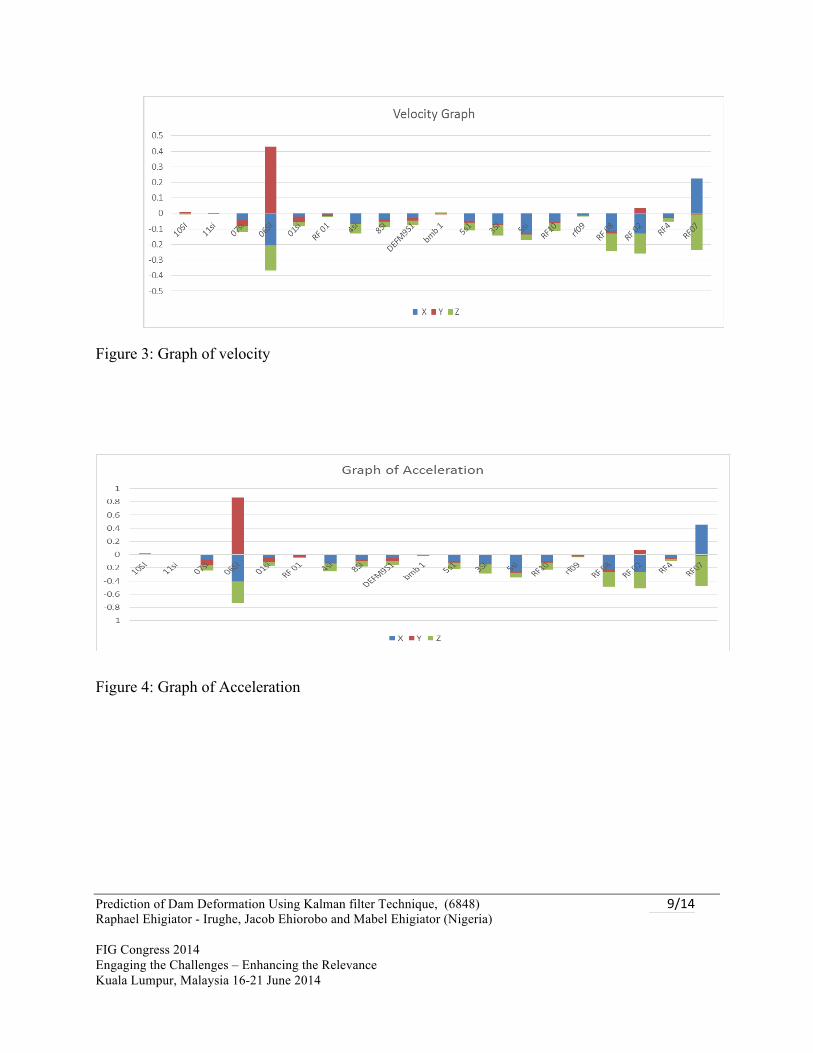
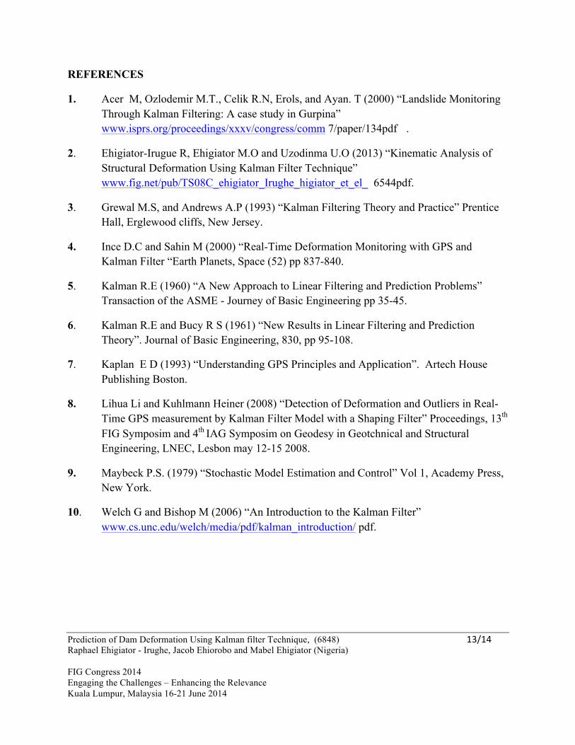
Fig 3 and 4 presents the graph of the velocity and acceleration of motion for each points in the network in the X, Y, and Z direction. In table 2, the predicted coordinates using the Kinematic model for each of the points for 2008 to 2013 is presented. A comparison of the measured and predicted coordinates for 2008 is presented in table 3 and represented graphically in figure 5.

Table 1: GPS measurement Results for 2007 and 2008 measurement period with velocity and acceleration.

Name North1 East1 Elev1. ΔN ΔE ΔZ North2 East2 Elev2. X Y Z X Y Z10SI 262870.5510 357263.0960 39.8850 -‐0.0011 0.0051 -‐0.0006 262870.5499 357263.1011 39.8844 -‐0.0022 0.0102 -‐0.0012 -‐0.0044 0.0204 -‐0.002411si 262868.8650 357204.4860 44.2180 0.0001 -‐0.0001 0.0000 262868.8651 357204.4859 44.2180 0.0002 -‐0.0002 0.0000 0.0004 -‐0.0004 0.000007si 262941.0620 357201.6470 44.0220 -‐0.0193 -‐0.0199 -‐0.0210 262941.0427 357201.6271 44.0010 -‐0.0386 -‐0.0398 -‐0.0420 -‐0.0772 -‐0.0796 -‐0.084006SI 262979.7740 357251.3880 39.5500 -‐0.1024 0.2157 -‐0.0822 262979.6716 357251.6037 39.4678 -‐0.2048 0.4314 -‐0.1644 -‐0.4096 0.8628 -‐0.328801si 263110.1890 357066.4360 50.3060 -‐0.0109 -‐0.0181 -‐0.0124 263110.1781 357066.4179 50.2936 -‐0.0218 -‐0.0362 -‐0.0248 -‐0.0436 -‐0.0724 -‐0.0496RF 01 262965.1170 357267.5310 38.4610 -‐0.0027 -‐0.0063 -‐0.0032 262965.1143 357267.5247 38.4578 -‐0.0054 -‐0.0126 -‐0.0064 -‐0.0108 -‐0.0252 -‐0.01284si 263386.1340 357865.5420 39.4500 -‐0.0298 -‐0.0038 -‐0.0304 263386.1042 357865.5382 39.4196 -‐0.0596 -‐0.0076 -‐0.0608 -‐0.1192 -‐0.0152 -‐0.12168SI 263080.3670 357964.0030 42.8980 -‐0.0182 -‐0.0080 -‐0.0184 263080.3488 357963.9950 42.8796 -‐0.0364 -‐0.0160 -‐0.0368 -‐0.0728 -‐0.0320 -‐0.0736

DEFM9S1 263035.9700 357904.9320 39.2710 -‐0.0143 -‐0.0098 -‐0.0143 263035.9557 357904.9222 39.2567 -‐0.0286 -‐0.0196 -‐0.0286 -‐0.0572 -‐0.0392 -‐0.0572bmb 1 263076.9420 357885.7800 38.3150 -‐0.0016 -‐0.0010 0.0023 263076.9404 357885.7790 38.3173 -‐0.0032 -‐0.0020 0.0046 -‐0.0064 -‐0.0040 0.00925s1 263175.6980 357933.4640 40.1760 -‐0.0231 -‐0.0076 -‐0.0239 263175.6749 357933.4564 40.1521 -‐0.0462 -‐0.0152 -‐0.0478 -‐0.0924 -‐0.0304 -‐0.09563SI 263444.5660 357851.6970 40.0370 -‐0.0344 -‐0.0026 -‐0.0348 263444.5316 357851.6944 40.0022 -‐0.0688 -‐0.0052 -‐0.0696 -‐0.1376 -‐0.0104 -‐0.13925si 263175.7010 357933.4640 40.2110 -‐0.0645 -‐0.0040 -‐0.0184 263175.6365 357933.4600 40.1926 -‐0.1290 -‐0.0080 -‐0.0368 -‐0.2580 -‐0.0160 -‐0.0736RF10 263068.5370 357839.7480 37.9670 -‐0.0260 -‐0.0051 -‐0.0253 263068.5110 357839.7429 37.9417 -‐0.0520 -‐0.0102 -‐0.0506 -‐0.1040 -‐0.0204 -‐0.1012rf09 263050.9580 357741.3140 37.8450 -‐0.0050 -‐0.0022 -‐0.0036 263050.9530 357741.3118 37.8414 -‐0.0100 -‐0.0044 -‐0.0072 -‐0.0200 -‐0.0088 -‐0.0144RF 08 263033.5000 357642.8350 37.8190 -‐0.0566 -‐0.0081 -‐0.0571 263033.4434 357642.8269 37.7619 -‐0.1132 -‐0.0162 -‐0.1142 -‐0.2264 -‐0.0324 -‐0.2284RF 02 262978.5430 357341.2900 37.9150 -‐0.0645 0.0173 -‐0.0641 262978.4785 357341.3073 37.8509 -‐0.1290 0.0346 -‐0.1282 -‐0.2580 0.0692 -‐0.2564RF4 263014.3530 357537.9720 37.9250 -‐0.0125 -‐0.0024 -‐0.0113 263014.3405 357537.9696 37.9137 -‐0.0250 -‐0.0048 -‐0.0226 -‐0.0500 -‐0.0096 -‐0.0452RF07 263047.2180 357567.5600 37.9020 0.1130 -‐0.0040 -‐0.1135 263047.3310 357567.5560 37.7885 0.2260 -‐0.0080 -‐0.2270 0.4520 -‐0.0160 -‐0.4540

2007 Measurement Displacement Velocity Acceleration2008 Measurement


9/14 Predicti

Figure 3: Graph of velocity

Figure 4: Graph of Acceleration


10/14

Table 2: Prediction

Table 3: Prediction and Correlation

Name North2 East2 Elev2. X Y Z ΔN ΔE ΔZ10SI 262870.5499 357263.101 39.8844 262871 357263 39.8838 0.0011 -‐0.0051 0.000611si 262868.8651 357204.486 44.218 262869 357204 44.218 -‐0.0001 0.0001 007si 262941.0427 357201.627 44.001 262941 357202 43.98 0.0193 0.0199 0.02106SI 262979.6716 357251.604 39.4678 262980 357252 39.3856 0.1024 -‐0.2157 0.082201si 263110.1781 357066.418 50.2936 263110 357066 50.2812 0.0109 0.0181 0.0124RF 01 262965.1143 357267.525 38.4578 262965 357268 38.4546 0.0027 0.0063 0.00324si 263386.1042 357865.538 39.4196 263386 357866 39.3892 0.0298 0.0038 0.03048SI 263080.3488 357963.995 42.8796 263080 357964 42.8612 0.0182 0.008 0.0184

DEFM9S1 263035.9557 357904.922 39.2567 263036 357905 39.2424 0.0143 0.0098 0.0143bmb 1 263076.9404 357885.779 38.3173 263077 357886 38.3196 0.0016 0.001 -‐0.00235s1 263175.6749 357933.456 40.1521 263176 357933 40.1282 0.0231 0.0076 0.02393SI 263444.5316 357851.694 40.0022 263444 357852 39.9674 0.0344 0.0026 0.03485si 263175.6365 357933.46 40.1926 263176 357933 40.1742 0.0645 0.004 0.0184RF10 263068.511 357839.743 37.9417 263068 357840 37.9164 0.026 0.0051 0.0253rf09 263050.953 357741.312 37.8414 263051 357741 37.8378 0.005 0.0022 0.0036RF 08 263033.4434 357642.827 37.7619 263033 357643 37.7048 0.0566 0.0081 0.0571RF 02 262978.4785 357341.307 37.8509 262978 357341 37.7868 0.0645 -‐0.0173 0.0641RF4 263014.3405 357537.97 37.9137 263014 357538 37.9024 0.0125 0.0024 0.0113RF07 263047.331 357567.556 37.7885 263047 357568 37.675 -‐0.113 0.004 0.1135

2008 Measurement Prediction for 2008 Correlation


11/14

Figure 5: Graph of correlation for year 2008 The computed displacements for Kinematic observation i.e ∆N, ∆E, and ∆Z show that all the points in the network moved except point 11SI, which has a vertical displacement of zero and horizontal shift of 0.14mm.

Maximum horizontal movement of 238mm and vertical movement of 82.2mm occurred in point 6S1 followed by reference point RF 7 with horizontal displacement of 113mm and vertical displacement of 113mm.

Maximum velocity and acceleration occurred in point 6SI for vertical and RF 7 for horizontal. Analysis of the results between the measurement update and predicted deformation results for 2008 indicate a correlation between the two, except in the case of 6SI and RF 7 where the correlation were weak.

An evaluation of the quality of the solution of the Kinematic model problem by Kalman filter using test statistics is the subject of discussions in another paper and have not been included here.

5. CONCLUSIONS

In this study, the Kalman filter technique based on Kinematic Deformation analysis was applied to measurement data collection by static GPS at the Ikpoba River Dam in Benin City, Nigeria.

By comparing the predicted and measured displacements, the efficiency of the Kinematic deformation model using Kalman filter was demonstrated. A major advantage in the method is


12/14

the ability to carry out step wise computation of structural movement parameters which projects forward the expected deformation at any later time.

This study focused on geodetic deformation prediction process using measurement parameters. The graph of correlation reveals that the accuracy of the predicted deformation compared quite well with the measured deformation for 2008. Further research is on going in order to determine the behavior for longer prediction period based on measured displacement.


13/14

REFERENCES

1. Acer M, Ozlodemir M.T., Celik R.N, Erols, and Ayan. T (2000) “Landslide Monitoring Through Kalman Filtering: A case study in Gurpina” www.isprs.org/proceedings/xxxv/congress/comm 7/paper/134pdf .

2. Ehigiator-Irugue R, Ehigiator M.O and Uzodinma U.O (2013) “Kinematic Analysis of Structural Deformation Using Kalman Filter Technique” www.fig.net/pub/TS08C_ehigiator_Irughe_higiator_et_el_ 6544pdf.

3. Grewal M.S, and Andrews A.P (1993) “Kalman Filtering Theory and Practice” Prentice Hall, Erglewood cliffs, New Jersey.

4. Ince D.C and Sahin M (2000) “Real-Time Deformation Monitoring with GPS and Kalman Filter “Earth Planets, Space (52) pp 837-840.

5. Kalman R.E (1960) “A New Approach to Linear Filtering and Prediction Problems” Transaction of the ASME - Journey of Basic Engineering pp 35-45.

6. Kalman R.E and Bucy R S (1961) “New Results in Linear Filtering and Prediction Theory”. Journal of Basic Engineering, 830, pp 95-108.

7. Kaplan E D (1993) “Understanding GPS Principles and Application”. Artech House Publishing Boston.

8. Lihua Li and Kuhlmann Heiner (2008) “Detection of Deformation and Outliers in Real-Time GPS measurement by Kalman Filter Model with a Shaping Filter” Proceedings, 13th FIG Symposim and 4th IAG Symposim on Geodesy in Geotchnical and Structural Engineering, LNEC, Lesbon may 12-15 2008.

9. Maybeck P.S. (1979) “Stochastic Model Estimation and Control” Vol 1, Academy Press, New York.

10. Welch G and Bishop M (2006) “An Introduction to the Kalman Filter” www.cs.unc.edu/welch/media/pdf/kalman_introduction/ pdf.


14/14

BIOGRAPHICAL NOTES

Dr. Raphael Irughe Ehigiator holds a BSc Surveying Geodesy and Photogrammetry from the University of Nigeria Nsukka, M.Eng Water Resources and Environmental Systems Engineering from the University of Benin and a PhD; Geomatics Engineering, from the Siberian State Geodesy Academy Novosibirsk Russia Federation. He is a corporate member of the Nigerian Institution of Surveyors (MNIS), and a Registered Surveyor in Nigeria. He is also a member of the Nigerian Association of Geodesy. He has worked extensively in the oil and gas industry in Nigeria. His research interest include; Deformation, Monitoring and Analysis, Precision Engineering Surveys, GNSS and Sensors Positioning, Terrestrial laser scanning e.t.c.

CONTACTS

Address: GeoSystems and Environmental Engineering, 140 2nd East Circular Road, Benin City, Edo State Nigeria. Tel: +2348033681019, Email: [email protected]

Dr. Jacob Ehiorobo is an Associate Professor in the Department of Civil Engineering, University of Benin. He holds an MSc Surveying Engineering Degree from MIIGAIK (Moscow), PhD from the University of Benin. He is a corporate member of the Nigerian Institution of Surveyors (MNIS), and a registered Surveyor in Nigeria. He is also a member of the Nigerian Association of Geodesy. His Research interests include Precision Engineering, Surveys, Deformation Measurement and Analysis, GNSS Positioning, Application of Sensors Technologies in Environmental Hazard Monitoring and Analysis. Flood and Erosion Monitoring and Control, and Water Resources Modelling and Management.

Dr. (Mrs) Mabel Ehigiator holds B.Sc degree in pure and applied Physics, Postgraduate diploma in Petroleum Engineering and an M.Sc degree in Exploration Geophysics from the University of Benin. A PhD in Geophysics at the Ambrose Ali University Ekpoma Edo State. She is a lecturer and Head of Department of Basic and Applied Sciences at the Benson Idahosa University, Benin City. Her research interests are Environmental geophysics, Subsidence and deformation, Exploration Geophysics, formation evaluation and reservoir geophysics.

Documents

Prediction of Dam Deformation Using Kalman Filter Technique · PDF file · 2014-07-03Prediction of Dam Deformation Using Kalman filter Technique, ... of time and varying loads