Prediction-based Resource Allocation using LSTM and minimum cost and maximum flow algorithm

Gyunam Park,�Minseok Song†

POSTECH,�Pohang,�South�Korea

June 26,�2019

Contents

• Introduction

• Background

• Method

• Evaluation

• Conclusion

2

Introduction

- Research Background

- Objective

3

• Resource allocation in business process management (BPM)

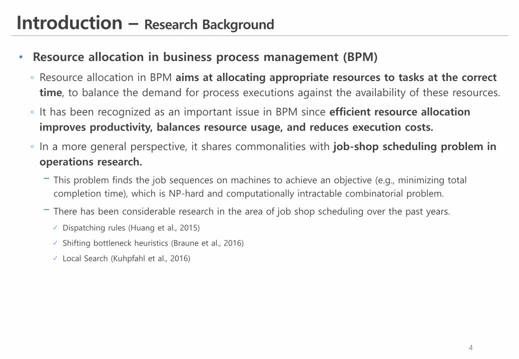
◦ Resource allocation in BPM aims at allocating appropriate resources to tasks at the correct time, to balance the demand for process executions against the availability of these resources.

◦ It has been recognized as an important issue in BPM since efficient resource allocation improves productivity, balances resource usage, and reduces execution costs.

◦ In a more general perspective, it shares commonalities with job-shop scheduling problem in operations research.

! This problem finds the job sequences on machines to achieve an objective (e.g., minimizing total completion time), which is NP-hard and computationally intractable combinatorial problem.

! There has been considerable research in the area of job shop scheduling over the past years.

Dispatching rules (Huang et al., 2015)

Shifting bottleneck heuristics (Braune et al., 2016)

Local Search (Kuhpfahl et al., 2016)

Introduction – Research Background

4

Introduction – Research Background

5

• Resource allocation in business process management (BPM)

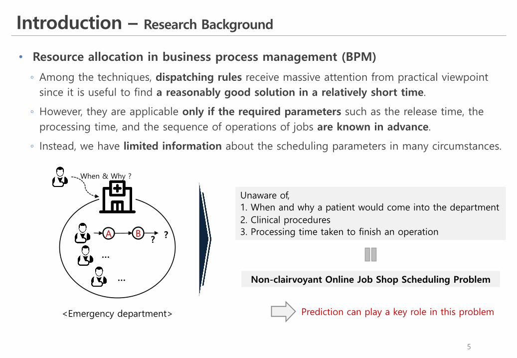
◦ Among the techniques, dispatching rules receive massive attention from practical viewpoint since it is useful to find a reasonably good solution in a relatively short time.

◦ However, they are applicable only if the required parameters such as the release time, the processing time, and the sequence of operations of jobs are known in advance.

◦ Instead, we have limited information about the scheduling parameters in many circumstances.

Unaware of,1. When and why a patient would come into the department2. Clinical procedures3. Processing time taken to finish an operation

When & Why ?

A B ??

…

… Non-clairvoyant Online Job Shop Scheduling Problem

<Emergency department> Prediction can play a key role in this problem

Introduction – Research Background

6

• Motivating example

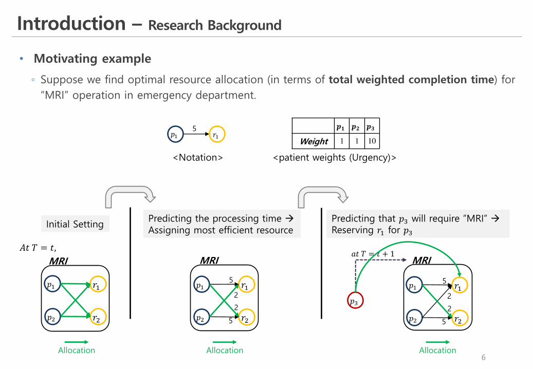
◦ Suppose we find optimal resource allocation (in terms of total weighted completion time) for “MRI” operation in emergency department.

𝒑𝟏 𝒑𝟐 𝒑𝟑

Weight 1 1 10𝑟&𝑝&

<patient weights (Urgency)>

5

2

5

2𝑝&

𝑝(

𝑟&

𝑟(

Predicting the processing time àAssigning most efficient resource

𝑝&

𝑝(

𝑟&

𝑟(

Initial Setting

𝑝&

𝑝(

𝑟&

𝑟(

𝑝)

Predicting that 𝑝) will require ”MRI” àReserving 𝑟& for 𝑝)

5

2

5

2

<Notation>

Allocation Allocation

5

MRI MRI MRI𝐴𝑡 𝑇 = 𝑡,

𝑎𝑡 𝑇 = 𝑡 + 1

Allocation

Introduction – Objective

7

Predictive business process monitoring Min-cost and max-flow algorithm

Prediction model

Historic data

1. Constructing prediction

model

Next Activity and processing time

Current data

2. Predicting parameters

Optimal Schedule

3. Scheduling

Resource allocation

4. Executing resource allocation

Phase 1: Offline prediction model

construction

Phase 2: Online resource scheduling

Prediction results

Resource Allocation (Non-clairvoyant Online Job Shop Scheduling)

Business Process ImprovementUtilized in Achieves

Background

- Preliminaries

- Problem Statement

- Baseline approach

8

Background – Preliminaries

9

• Predictive business process monitoring

◦ Predictive business process monitoring aims at providing timely information that enable proactive and corrective actions to improve process performance and mitigate risks.

! Next event prediction: predicting the next event of a running instance such as next activity.

! Time prediction: predicting time-related properties of a running instance such as remaining time and processing time.

◦ Tax et al. (2017) propose an approach that predicts both the next activity and its timestamp using LSTM (Long-Short Term Memory Neural Network).

LSTM(Long-Short Term Memory)- Sequence learning tasks

(e.g., Natural language processing (NLP) )

- Learning temporal dynamics

LSTM

Next Activityprediction

Timeprediction

Feature vector

LSTM

LSTM LSTM

LSTM LSTM

Event Log

• Minimum cost and maximum flow problem

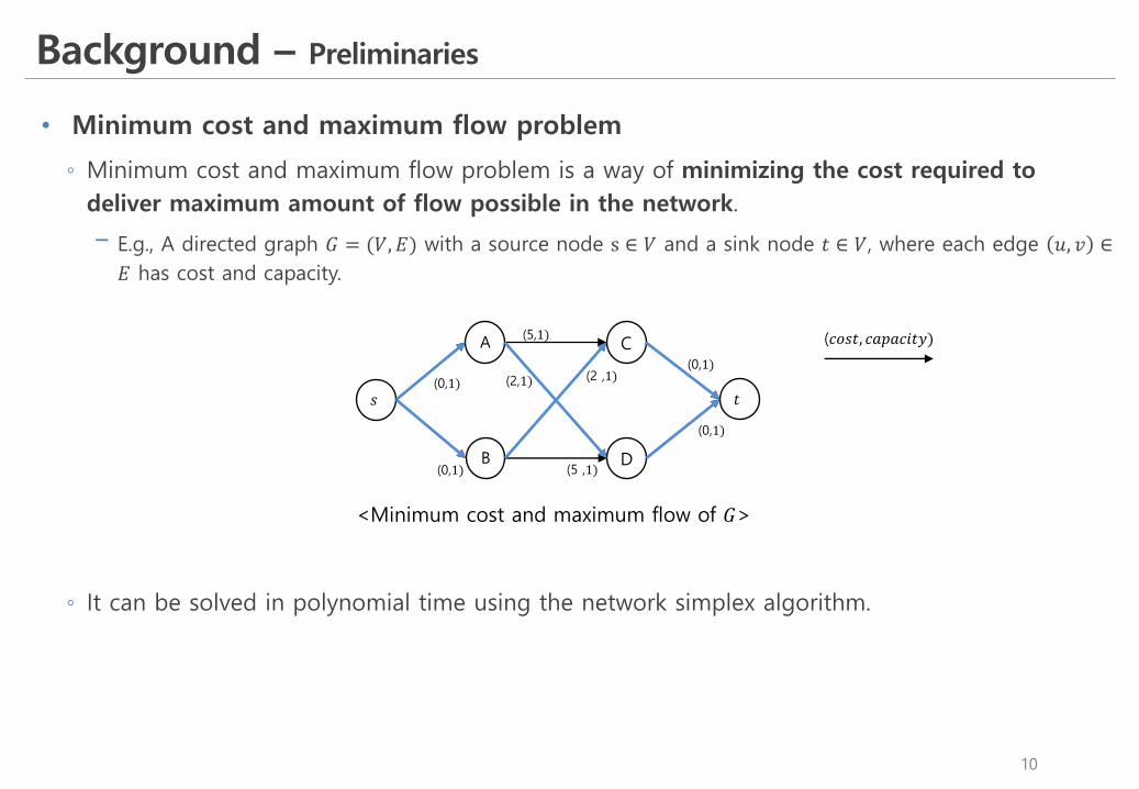
◦ Minimum cost and maximum flow problem is a way of minimizing the cost required to deliver maximum amount of flow possible in the network.

! E.g., A directed graph 𝐺 = (𝑉, 𝐸) with a source node s ∈ 𝑉 and a sink node 𝑡 ∈ 𝑉, where each edge 𝑢, 𝑣 ∈𝐸 has cost and capacity.

◦ It can be solved in polynomial time using the network simplex algorithm.

Background – Preliminaries

10

A

B

C

D

(5,1)

(2,1)

(5 ,1)

(2 ,1)

𝑠 𝑡(0,1)

(0,1)

(0,1)

(0,1)

<Minimum cost and maximum flow of 𝐺>

(𝑐𝑜𝑠𝑡, 𝑐𝑎𝑝𝑎𝑐𝑖𝑡𝑦)

Background – Problem Statement

11

• Non-clairvoyant Online Job Shop Scheduling Problem

◦ Given a set of instances I, this problem finds an optimal scheduling of all operations within instances while minimizing total weighted completion time 𝚺𝒊𝒘𝒊𝑪𝒊,

! 𝑤E: weight of 𝐼E! 𝐶E: difference between the finish time 𝐹E and start time 𝑆E of an instance 𝐼E.

◦ Assumptions:1. Unaware of the information regarding an instance except the weight of it.

2. Find out the next operation of an instance only if the instance finishes its current operation.

3. Each operation has a specific set of resources with whom it needs to be processed.

4. Only one operation within an instance can be processed at a given time.

5. Once processing begins on an operation, it cannot be stopped until completion.

Background – Problem Statement

12

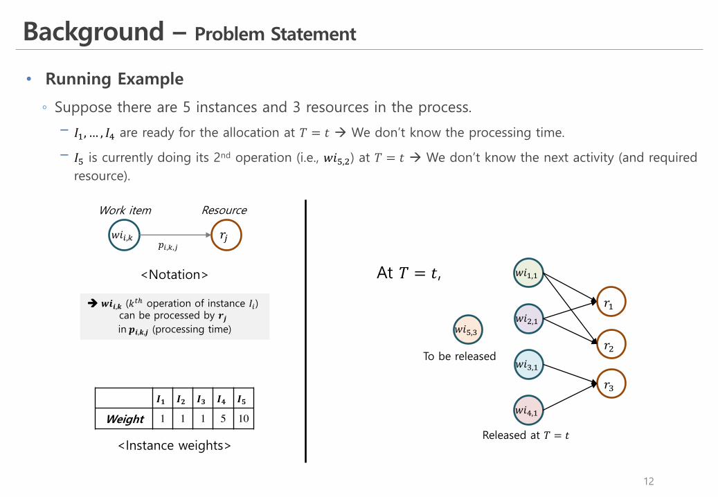
• Running Example

◦ Suppose there are 5 instances and 3 resources in the process.

! 𝐼&, … , 𝐼K are ready for the allocation at 𝑇 = 𝑡 à We don’t know the processing time.

! 𝐼L is currently doing its 2nd operation (i.e., 𝑤𝑖L,() at 𝑇 = 𝑡 à We don’t know the next activity (and required resource).

𝑤𝑖&,&

𝑤𝑖(,&

𝑤𝑖),&

𝑟&

𝑟(

𝑟)

𝑤𝑖L,)

Released at 𝑇 = 𝑡

𝑤𝑖K,&

To be released

<Notation>

𝑤𝑖E,M 𝑟N

Work item Resource

𝑝E,M,N

<Instance weights>

𝑰𝟏 𝑰𝟐 𝑰𝟑 𝑰𝟒 𝑰𝟓

Weight 1 1 1 5 10

à 𝒘𝒊𝒊,𝒌 (𝑘TU operation of instance 𝐼E) can be processed by 𝒓𝒋in 𝒑𝒊,𝒌,𝒋 (processing time)

At 𝑇 = 𝑡,

Background – Baseline approach

13

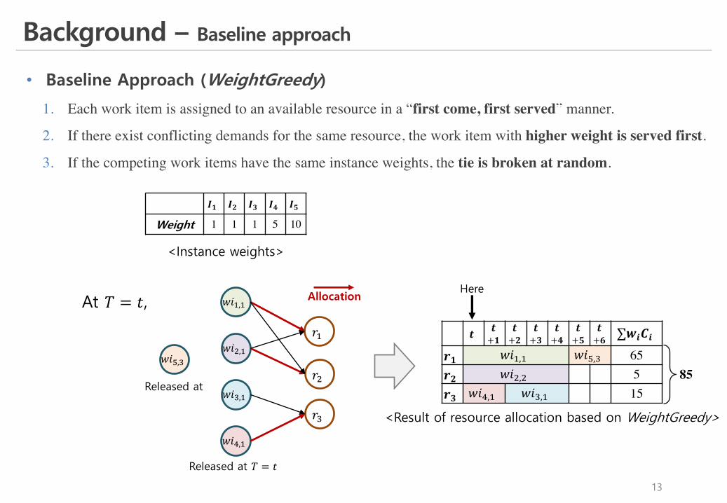
• Baseline Approach (WeightGreedy)

1. Each work item is assigned to an available resource in a “first come, first served” manner.

2. If there exist conflicting demands for the same resource, the work item with higher weight is served first.

3. If the competing work items have the same instance weights, the tie is broken at random.

𝑤𝑖&,&

𝑤𝑖(,&

𝑤𝑖),&

𝑟&

𝑟(

𝑟)

𝑤𝑖L,)

Released at 𝑇 = 𝑡

𝑤𝑖K,&

Released at

At 𝑇 = 𝑡,

𝒕 𝒕+𝟏

𝒕+𝟐

𝒕+𝟑

𝒕+𝟒

𝒕+𝟓

𝒕+𝟔 ∑𝒘𝒊𝑪𝒊

𝒓𝟏 𝑤𝑖&,& 𝑤𝑖L,) 65𝒓𝟐 𝑤𝑖(,( 5𝒓𝟑 𝑤𝑖K,& 𝑤𝑖),& 15

<Result of resource allocation based on WeightGreedy>

<Instance weights>

𝑰𝟏 𝑰𝟐 𝑰𝟑 𝑰𝟒 𝑰𝟓

Weight 1 1 1 5 10

85

AllocationHere

Method

- Overview

- Steps

14

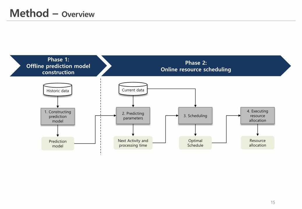
Method – Overview

15

Prediction model

Historic data

1. Constructing prediction

model

Next Activity and processing time

Current data

2. Predicting parameters

Optimal Schedule

3. Scheduling

Resource allocation

4. Executing resource allocation

Phase 1: Offline prediction model

construction

Phase 2: Online resource scheduling

Method – Phase 1

16

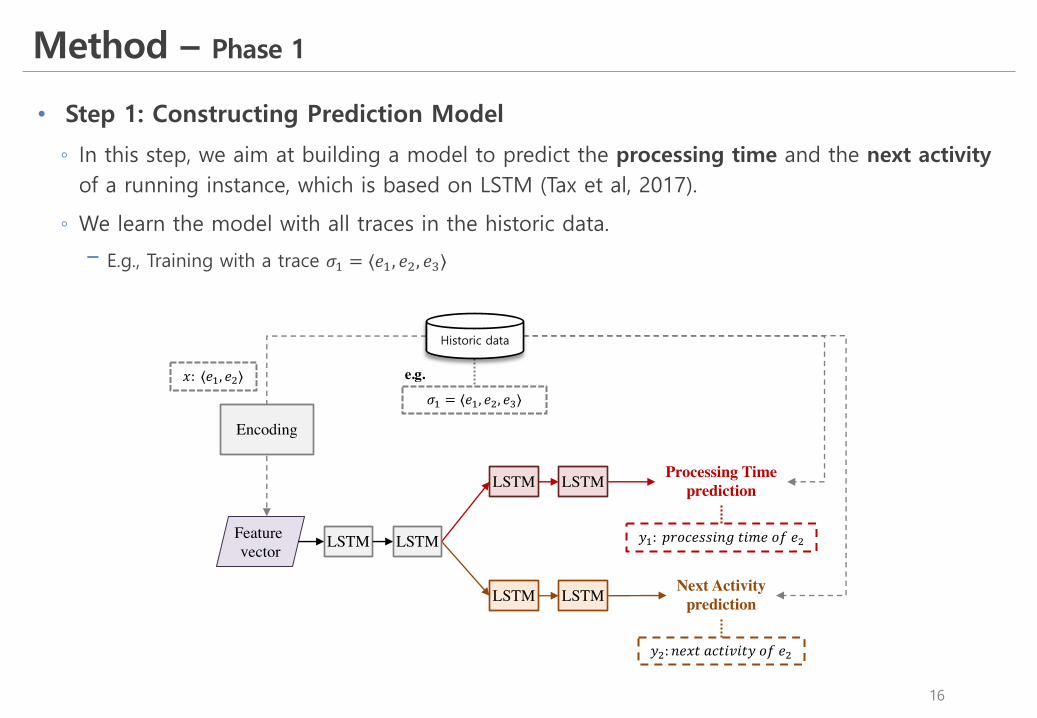
• Step 1: Constructing Prediction Model

◦ In this step, we aim at building a model to predict the processing time and the next activity of a running instance, which is based on LSTM (Tax et al, 2017).

◦ We learn the model with all traces in the historic data.

! E.g., Training with a trace 𝜎& = ⟨𝑒&, 𝑒(, 𝑒)⟩

LSTM

Next Activityprediction

Processing Timeprediction

Feature vector

𝑦(: 𝑛𝑒𝑥𝑡 𝑎𝑐𝑡𝑖𝑣𝑖𝑡𝑦 𝑜𝑓 𝑒(

𝑦&: 𝑝𝑟𝑜𝑐𝑒𝑠𝑠𝑖𝑛𝑔 𝑡𝑖𝑚𝑒 𝑜𝑓 𝑒(

𝜎& = ⟨𝑒&, 𝑒(, 𝑒)⟩

LSTM

LSTM

LSTM

LSTM

LSTM

e.g.

Encoding

𝑥: ⟨𝑒&, 𝑒(⟩

Historic data

Method – Phase 2

17

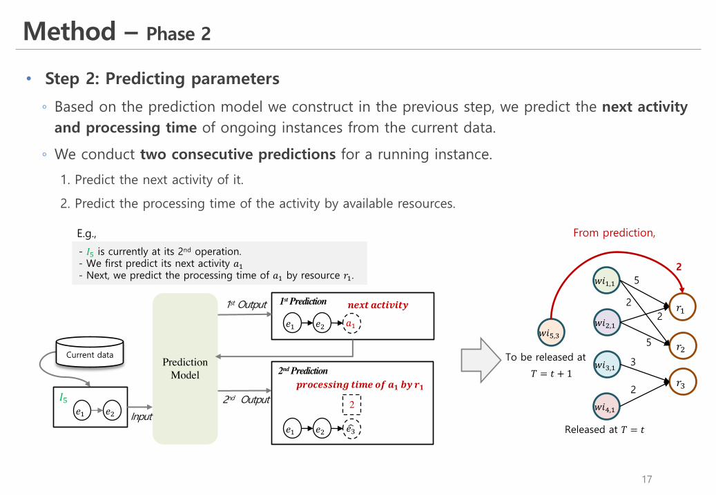
• Step 2: Predicting parameters

◦ Based on the prediction model we construct in the previous step, we predict the next activity and processing time of ongoing instances from the current data.

◦ We conduct two consecutive predictions for a running instance.

1. Predict the next activity of it.

2. Predict the processing time of the activity by available resources.

Prediction Model

𝑎&

𝐼L𝑒& 𝑒( Input

1st Output

𝑒& 𝑒(

𝒏𝒆𝒙𝒕 𝒂𝒄𝒕𝒊𝒗𝒊𝒕𝒚

2nd Output

l𝑒)

2

𝒑𝒓𝒐𝒄𝒆𝒔𝒔𝒊𝒏𝒈 𝒕𝒊𝒎𝒆𝒐𝒇𝒂𝟏 𝒃𝒚 𝒓𝟏

𝑒& 𝑒(

1st Prediction

2nd PredictionCurrent data

𝑤𝑖&,&

𝑤𝑖(,&

𝑤𝑖),&

𝑟&

𝑟(

𝑟)

𝑤𝑖L,)

Released at 𝑇 = 𝑡

𝑤𝑖K,&

To be released at

𝑇 = 𝑡 + 1

5

2

5

3

2

2

- 𝐼L is currently at its 2nd operation.- We first predict its next activity 𝑎&- Next, we predict the processing time of 𝑎& by resource 𝑟&.

E.g.,

2

From prediction,

(0,1)

(0,1)

(0,1)

(0,1)

(0,1)

(0,1)

(0,1)

(0,1)

Method – Phase 2

18

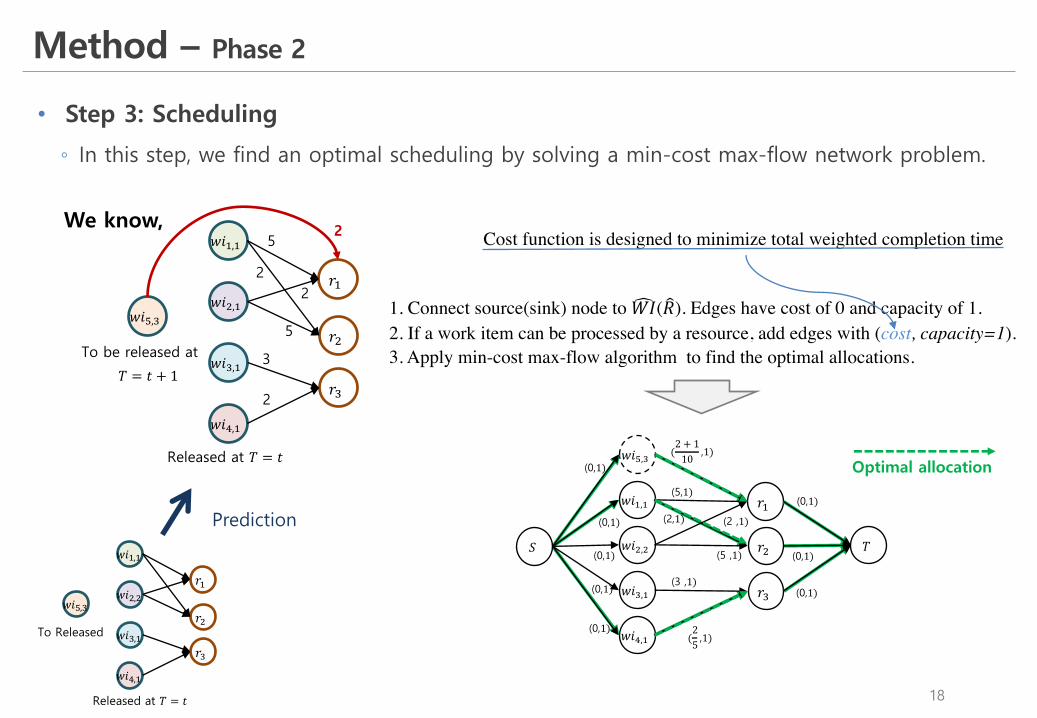
• Step 3: Scheduling

◦ In this step, we find an optimal scheduling by solving a min-cost max-flow network problem.

1. Connect source(sink) node to s𝑊𝐼( u𝑅). Edges have cost of 0 and capacity of 1.2. If a work item can be processed by a resource, add edges with (cost, capacity=1).3. Apply min-cost max-flow algorithm to find the optimal allocations.

Cost function is designed to minimize total weighted completion timeWe know,

𝑤𝑖&,&

𝑤𝑖(,(

𝑤𝑖),&

𝑟&

𝑟(

𝑟)

𝑤𝑖L,)

𝑤𝑖K,&

(5,1)

(2,1)

(5 ,1)

(3 ,1)

(2 ,1)

(2 + 110

,1)

(25 ,1)

𝑆 𝑇

Optimal allocation

𝑤𝑖&,&

𝑤𝑖(,(

𝑤𝑖),&

𝑟&

𝑟(

𝑟)

𝑤𝑖L,)

Released at 𝑇 = 𝑡

𝑤𝑖K,&

To Released

Prediction

𝑤𝑖&,&

𝑤𝑖(,&

𝑤𝑖),&

𝑟&

𝑟(

𝑟)

𝑤𝑖L,)

Released at 𝑇 = 𝑡

𝑤𝑖K,&

To be released at

𝑇 = 𝑡 + 1

5

2

5

3

2

2

2

Method – Phase 2

19

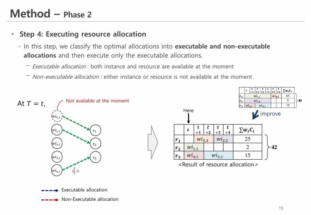
• Step 4: Executing resource allocation

◦ In this step, we classify the optimal allocations into executable and non-executable allocations and then execute only the executable allocations.

! Executable allocation : both instance and resource are available at the moment

! Non-executable allocation : either instance or resource is not available at the moment

𝑤𝑖&,&

𝑤𝑖(,(

𝑤𝑖),&

𝑟&

𝑟(

𝑟)

𝑤𝑖L,)

𝑤𝑖K,& (25

,1)

Non-Executable allocation

Executable allocation

At 𝑇 = 𝑡,

𝒕 𝒕+𝟏

𝒕+𝟐

𝒕+𝟑

𝒕+𝟒 ∑𝒘𝒊𝑪𝒊

𝒓𝟏 𝑤𝑖L,) 𝑤𝑖(,( 25𝒓𝟐 𝑤𝑖&,& 2𝒓𝟑 𝑤𝑖K,& 𝑤𝑖),& 15

42

Here

<Result of resource allocation>

Not available at the moment

improve

Evaluation

- Artificial event log

- Real-life event log

20

• Experimental design

◦ Procedure

1. Design a business process and generate historic data and current data by simulating it.

2. Compare our proposed method with baseline approach in terms of total weighted completion time and computation time by varying the number of instances.

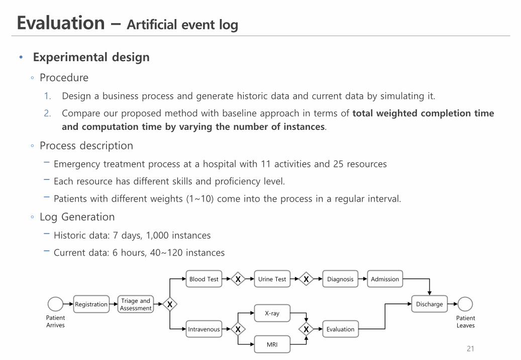
◦ Process description

! Emergency treatment process at a hospital with 11 activities and 25 resources

! Each resource has different skills and proficiency level.

! Patients with different weights (1~10) come into the process in a regular interval.

◦ Log Generation

! Historic data: 7 days, 1,000 instances

! Current data: 6 hours, 40~120 instances

Evaluation – Artificial event log

21

Registration Triage and Assessment

Blood Test

Intravenous

X

X

X

Urine Test

X-ray

MRI

X Evaluation

DiagnosisX Admission

Discharge

Patient Arrives

Patient Leaves

Evaluation – Artificial event log

22

• Results

◦ Total weighted completion time and computation time, given the different number of instances.

<Total weighted completion time of varying |I|> <Computation time of varying |I|>

- Baseline: 28,393- Suggested: 24,804 (-14%)

High computation for prediction

Evaluation – Real-life event log

23

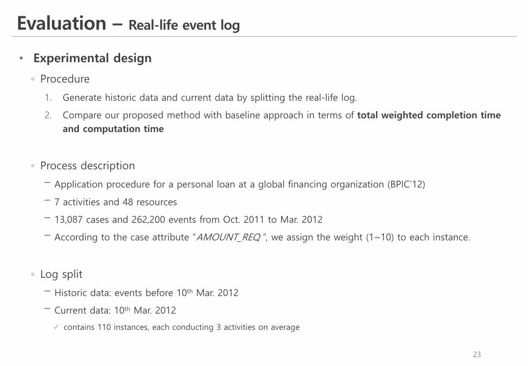
• Experimental design

◦ Procedure

1. Generate historic data and current data by splitting the real-life log.

2. Compare our proposed method with baseline approach in terms of total weighted completion time and computation time

◦ Process description

! Application procedure for a personal loan at a global financing organization (BPIC’12)

! 7 activities and 48 resources

! 13,087 cases and 262,200 events from Oct. 2011 to Mar. 2012

! According to the case attribute “AMOUNT_REQ ”, we assign the weight (1~10) to each instance.

◦ Log split

! Historic data: events before 10th Mar. 2012

! Current data: 10th Mar. 2012

contains 110 instances, each conducting 3 activities on average

Evaluation – Real-life event log

24

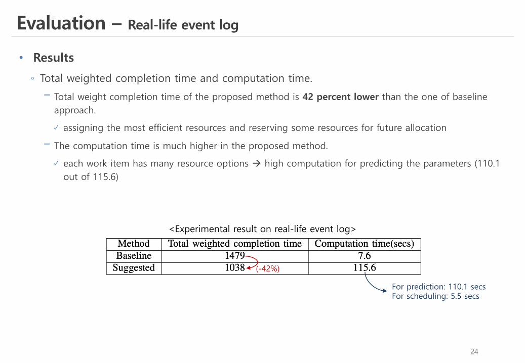
• Results

◦ Total weighted completion time and computation time.

! Total weight completion time of the proposed method is 42 percent lower than the one of baseline approach.

assigning the most efficient resources and reserving some resources for future allocation

! The computation time is much higher in the proposed method.

each work item has many resource options à high computation for predicting the parameters (110.1 out of 115.6)

<Experimental result on real-life event log>

(-42%)

For prediction: 110.1 secsFor scheduling: 5.5 secs

Conclusion

- Contribution

- Limitation

- Future works

25

Conclusion

26

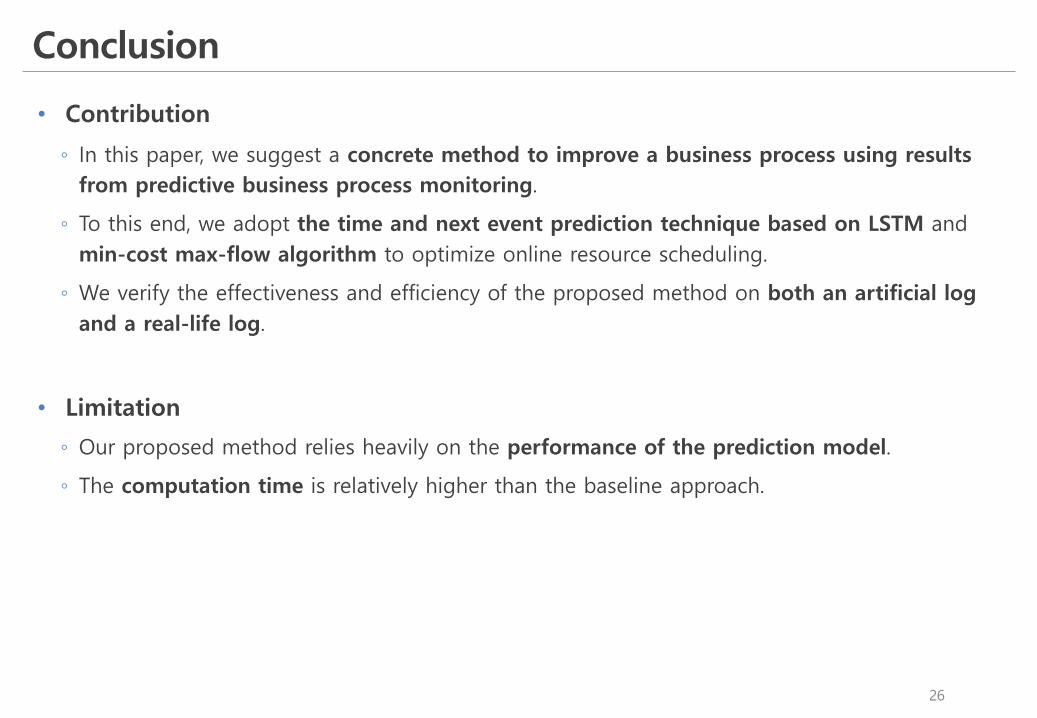
• Contribution

◦ In this paper, we suggest a concrete method to improve a business process using results from predictive business process monitoring.

◦ To this end, we adopt the time and next event prediction technique based on LSTM and min-cost max-flow algorithm to optimize online resource scheduling.

◦ We verify the effectiveness and efficiency of the proposed method on both an artificial log and a real-life log.

• Limitation

◦ Our proposed method relies heavily on the performance of the prediction model.

◦ The computation time is relatively higher than the baseline approach.

Conclusion

27

• Future work

◦ We will conduct additional experiments such as the effect of the prediction accuracy on the performance.

◦ We will extend this two-phase method to achieve another goal such as minimizing the potential risks in the business process by predicting other relevant parameters and defining a relevant cost function of network arcs.

◦ Another direction for future work is to extend the proposed method by adopting advanced dispatching techniques.

Q&A