European Water 57: 85-92, 2017. © 2017 E.W. Publications

Prediction and validation of turbulent flow around a cylindrical weir

N.G. Soydan, O. Şimşek* and M.S. Aköz Cukurova University, Civil Engineering Department, Adana, Turkey * e-mail: oguzsimsek@cu.edu.tr

Abstract: Weirs are commonly used for regulating, controlling and measuring the flow in a river or an open channel. When a weir is constructed across a river, sediment deposition occurs in the upstream of the structure and this can affect the function and efficiency of the weir. If these structures can be designed to pass sediment, the performance of the weir will not change over time because of sediment accumulation. In this study, the characteristics of turbulent flow around a cylindrical weir placed at a distance from the bed are investigated experimentally and numerically. The governing equations of the two-dimensional turbulent flow is solved numerically by using ANSYS Fluent. The volume of fluid (VOF) method is used to compute the free surface of the flow. Grid Convergence Index (GCI) is performed to examine the effect of the selected grid structure on the numerical results. In the numerical simulations, Renormalization Group k-ε, Shear Stress Transport k-w and Reynolds Stress turbulence closure models are employed. The numerical results for the turbulent flow characteristics are compared with the experimental data obtained by Laser Doppler Anemometer measurements in a laboratory channel. Experimental validations of the velocity field and free surface profiles show that the computations by using the turbulence models are successful in predicting the turbulent flow characteristics around a cylindrical weir placed at a distance from the bed.

Key words: Cylindrical Weir, Laser Doppler Anemometer, Open Channel Flow, Turbulence Model, VOF

1. INTRODUCTION

In open channel flow, weirs are commonly used for flow control and discharge measurement. Cylindrical weir is a construction which has many advantages such as stable overflow pattern, easy discharge, simple design and lower cost. Also, it has larger discharge capacity than the sharp crested and broad crested weirs (Chanson and Montes 1998). The flowing water in an open channel, transports sediment particles and these particles accumulate at the gate inlets and behind the weir structures. This can lead to overflowing of the water with narrowing the channel width, may cause the stability of the structure to deteriorate and reduce the measurement accuracy. Therefore, Majcherek (1984) first suggested an idea of combined-free over-under flow on a weir-gate. By using a model where weirs and gates are combined, sedimentation effects can be minimized. If the weir structure placed at a distance from the bed, it could be able to control the sediment transport and water level at the same time. While some attention has been focused on this topic, it has not yet been studied in detail experimentally and numerically. Chanson and Montes (1998), studied the circular weir overflows, with eight cylinder sizes, for several weir heights and for five types of inflow conditions experimentally. They stated from the range of the experiments that the cylinder size, the weir height D/R and the presence of an upstream ramp had no effect on the discharge coefficient, flow depth at crest, and energy dissipation. They concluded that the discharge measurements with circular weirs are significantly affected by the upstream flow conditions. Bhattacharyya and Maiti (2004), studied the vortex shedding around a cylinder and the Karman vortex street behind a cylinder experimentally and numerically. At Reynolds number up to 1400, the interaction of wall boundary layer on the vortex shedding has been investigated for different gap ratios. The governing equations of the unsteady flow are discretized by finite volume method. It has been found that the strength of the positive vortices arising from the lower side of the cylinder reduces with the decrease of gap height. Castro-Orgaz, et al. (2008), examined the hydraulics of circular crested weirs by using generalized one dimensional model based on the critical flow in

N.G. Soydan et al. 86

curvilinear motion which was developed by themselves. The predictions obtained from the models compared with the experimental results. They stated that the discharge coefficient increases when the streamline effects are included. Severi et al. (2015), experimentally studied on discharge coefficient variation of combined-free over-under flow on a cylindrical weir-gate. For varied geometrical dimensions of the weir-gate under hydraulic conditions of over, combined and under flows, many experiments were carried out. They used the Buckingham Phi theorem to correlate the discharge coefficient to the effective dimensionless hydraulic and geometrical arguments. They stated that the developed empirical relationships for over, combined and under flows presented good coincidence with experimental results within the limitations of the runs.

In this study the characteristics of flow over and under a cylindrical weir is investigated experimentally and numerically. The governing equations of the weir flow are solved by using ANSYS-Fluent program based on the finite volume method. In the numerical analysis Renormalization Group k-ε (RNG), Shear Stress Transport k-ω (SST) and Reynolds Stress Model (RSM) were used. The velocity field of the flow is measured by means of Laser Doppler Anemometry technique. The velocity field and free surface profiles of the weir flow are presented and discussed.

2. EXPERIMENTAL SET-UP

Experiments were conducted in a glass-walled, hydraulically smooth laboratory channel that was 0.30 m wide, 0.30 m deep and 8.00 m long. As may be seen in Figure 1, a smooth-surface cylindrical weir with D=0.16 m diameter was placed at 5 m distance from the beginning of the channel and 3 cm above the channel bed. The free surface profile of three-dimensional flow around a cylindrical weir was measured by using limnimetry. The velocity field around the weir was obtained by using one dimensional Laser Doppler Anemometry. The Reynolds number in the upstream region of the flow is calculated as 135575. The flow in the upstream of the channel is subcritical, with a Froude number of 0.254. The experiment is performed for a flow rate of 0.0317 m3/s.

Figure 1. Schematic view of open channel flow with cylindrical weir

3. FORMULATION AND NUMERICAL MODELING

3.1 Governing equations

The 2D Reynolds-averaged continuity and Navier-Stokes equations (RANS) were used to theoretically simulate the present open channel flow. For an incompressible, Newtonian fluid flow these equations can be expressed as

0xu

i

i =∂

∂ (1)

j

ij2j

i2

ii

j

ij

i

xxu

xpg

xuu

tu

∂

τ∂+

∂

∂µ+

∂

∂−ρ=⎟

⎟

⎠

⎞

⎜⎜

⎝

⎛

∂

∂+

∂

∂ρ (2)

D=16 cm

0.30 m

5 m 3 m

European Water 57 (2017) 87

In Eqs. (1) and (2), ui is velocity component in xi-direction, gi is gravity, p is pressure, µ is dynamic viscosity, ρ is fluid density, t is time, )uu( jiij ʹʹρ−=τ is the turbulence stress. The turbulence stresses are obtained from the linear constitutive equation formulated by Boussinesq:

iji

j

j

itjiij k

32

xu

xuuu δρ−⎟

⎟

⎠

⎞

⎜⎜

⎝

⎛

∂

∂+

∂

∂µ=ʹʹρ−=τ (3)

In Eq. (3) iuʹ and juʹ is horizontal and vertical velocity fluctuation, respectively, µt is turbulent

viscosity, k ( 2/uu ii ʹʹ= ) is the turbulent kinetic energy and ijδ is Kronecker delta. The models used for the calculation of the turbulent viscosity in Eq. (3) are:

1. Renormalization-group k-ε (RNG) (Yakhot et al. 1992), 2. Shear Stress Transport k-ω (SST) (Menter 1994), 3. Reynold Stress Model (RSM) (Launder et al. 1975)

3.2 Solution domain, boundary and initial conditions

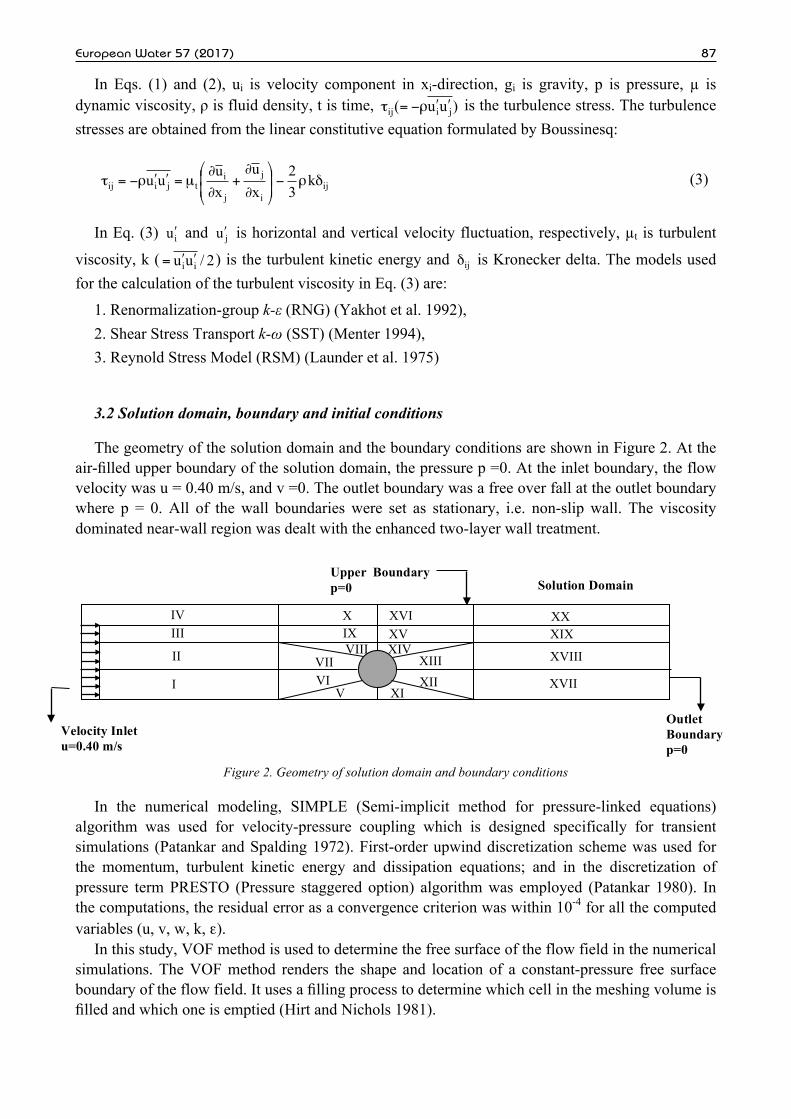
The geometry of the solution domain and the boundary conditions are shown in Figure 2. At the air-filled upper boundary of the solution domain, the pressure p =0. At the inlet boundary, the flow velocity was u = 0.40 m/s, and v =0. The outlet boundary was a free over fall at the outlet boundary where p = 0. All of the wall boundaries were set as stationary, i.e. non-slip wall. The viscosity dominated near-wall region was dealt with the enhanced two-layer wall treatment.

Figure 2. Geometry of solution domain and boundary conditions

In the numerical modeling, SIMPLE (Semi-implicit method for pressure-linked equations) algorithm was used for velocity-pressure coupling which is designed specifically for transient simulations (Patankar and Spalding 1972). First-order upwind discretization scheme was used for the momentum, turbulent kinetic energy and dissipation equations; and in the discretization of pressure term PRESTO (Pressure staggered option) algorithm was employed (Patankar 1980). In the computations, the residual error as a convergence criterion was within 10-4 for all the computed variables (u, v, w, k, ε).

In this study, VOF method is used to determine the free surface of the flow field in the numerical simulations. The VOF method renders the shape and location of a constant-pressure free surface boundary of the flow field. It uses a filling process to determine which cell in the meshing volume is filled and which one is emptied (Hirt and Nichols 1981).

III

II XIII

I

IV

V

VIII

VI

X IX

XII XI

Solution Domain

Outlet Boundary p=0

Upper Boundary p=0

Velocity Inlet u=0.40 m/s

VII XIV XV XVI

XVII

XVIII

XIX XX

N.G. Soydan et al. 88

3.3 Computational Grid

The resolution of the computational discretization of the solution domain is important for an ultimate grid-independent solution. For the purpose of designing a suitably-spaced computational grid system, structured grids of different local cell concentrations were tested. Considering the flow characteristics for the present interaction problem, the solution domain was divided into 20 regional sub-domains. Due to the increasing velocity gradient, the density of discretization was intentionally increased towards the solid boundary by compressing the grid system. Three grid systems with different density, Grid 1 (coarse), Grid 2 (medium) and Grid 3 (fine), were used to examine the effect of the grid size on the accuracy of the numerical results. Fine grid which is adopted for the final design of the computational grid system, containing 20 sub-domains, is seen in Figure 3. The discretization error of the computational domain was estimated using a Grid Convergence Index (GCI) for the three-grid comparisons (Roache (1998), Çelik, et al. (2008)). The predicted errors in the velocity due to discretization for the fine-grid solutions were found within 2% which is well acceptable for the verification of computed results. Therefore, the solution obtained on the fine mesh given in Figure 3 can be accepted as grid-independent.

Figure 3. Sub-domains of computational grid

4. RESULTS AND DISCUSSION

In the comparisons of computed velocity profiles from different turbulence closure models with those of experiments, mean square error (MSE) and mean absolute relative error (MARE) values were used as a quantitative evaluation criterion. MSE and MARE of measured and predicted velocity profiles in the channel is expressed as

2pm

N

1n)vv(

N1MSE −∑=

= (4)

100xvvv

N1MARE

N

1n m

pm∑

−=

=

(5)

where vm and vp are measured and computed mean horizontal velocities, respectively along the solution domain and N is the total number of velocity profiles. The results of MSE and MARE values calculated for the velocity profiles from the different turbulence closure models are given in Table I. From the table, it can be seen that according to the mean MSE and MARE values the most successful turbulence model in predicting the velocity field around the cylindrical weir is RNG turbulence model. RNG model shows superior performance in the upstream, downstream and upper region of the cylindrical weir among the used models. Figure 4 shows the experimental x velocity distribution around the cylindrical weir. From the figure, the stagnation region effect on the x velocity profile can be clearly seen in the upstream region. The jet flow formation under the

I

II

III

IV

V

VI VII

VIII

XI

X

XI

XII XIII

XIV

XV

XVI

XVII

XVIII

XIX

XX

European Water 57 (2017) 89

cylindrical weir, the effect of streamline curvature over the weir and the distribution of the velocity profile in the wake region behind the circular weir are also clearly evident from the figure. The graphical comparisons of the horizontal velocity profiles between the experimental data and numerical predictions using the turbulence models in the upstream and downstream region of the cylindrical weir were also given in Figure 5. It can be clearly seen that all the turbulence models show discrepancies with the experimental measurements near the wall region in the upstream region of the weir. In the downstream region the poor agreement between the experimental and numerical velocity profiles can be clearly seen.

Table 1. MSE and MARE values for the horizontal velocity profiles at different sections for the turbulence models

x(cm) RNG RSM SST MARE MSE MARE MSE MARE MSE

420 7.119 0.001 8.568 0.001 7.732 0.001 468 7.201 0.001 8.971 0.001 7.837 0.001 484 7.908 0.002 10.828 0.004 8.802 0.003 487 9.131 0.004 13.752 0.007 11.062 0.005 490 15.085 0.006 21.124 0.012 17.796 0.008 491 21.858 0.012 28.172 0.021 24.942 0.016 492 17.594 0.017 24.414 0.030 20.908 0.023 494 42.672 0.157 47.106 0.176 44.487 0.164 500 12.445 0.047 18.210 0.102 15.261 0.071 506 58.068 0.161 72.709 0.195 64.214 0.165 508 58.242 0.065 77.153 0.092 59.858 0.070 510 482.380 0.132 547.640 0.160 495.058 0.138 512 59.117 0.131 65.305 0.156 60.383 0.134 514 40.339 0.186 42.423 0.201 39.341 0.179 516 28.654 0.160 31.272 0.187 28.336 0.157 525 30.673 0.246 33.253 0.283 30.711 0.243 548 26.840 0.203 28.762 0.229 27.274 0.206

Mean 54.431 0.090 63.510 0.109 56.706 0.093

Figure 4. Experimental x velocity distribution around the cylindrical weir

Figure 6 gives the measured and computed free surface profiles from the VOF method along the channel by the three turbulence models used in this study. As may be seen from the figures, the computed flow profile using all turbulence models show good agreement with the measured profile throughout the solution domain. In the upstream and downstream regions, the differences between the predictions and measurements can be clearly seen from the figure. In the weir region turbulence models show good agreements with the measurement. Figure 7 shows the plan view of the x and y velocity components obtained from RNG turbulence model in the weir region. From the contours of x velocity, the stagnation point in front of the weir is clearly seen. Also, the wake region in the downstream region where the maximum pressure and minimum velocity occurs can be seen. The maximum values of the x velocity component are located under the cylindrical weir where the jet flow occurs. The contours of y velocity show where the two dimensional flow is prominent. The maximum y velocity occurs where the flow goes over the weir as expected.

5.0 4.9 4.8 5.1 5.2 5.3 4.7 x (m)

N.G. Soydan et al. 90

Figure 5. The experimental and predicted horizontal velocity profiles obtained by the three different turbulence closure models for selected sections

Figure 8 gives the streamline patterns and velocity vectors of the flow field around the cylindrical weir obtained from RNG turbulence model which is found to be the most successful model in this study. As may be seen from the streamline patterns and velocity vectors, RNG turbulence model predict successfully the stagnation region in the upstream face, jet flow under the weir, streamline curvature effect over the weir and the wake region behind the weir successfully. Figure 9 gives the numerical turbulence kinetic energy (TKE) and the pressure distribution along the channel and around the cylindrical weir obtained from RNG turbulence model. It can be clearly seen from the patterns of turbulence kinetic energy contours that the maximum value of the turbulence kinetic energy is calculated under the cylindrical weir where the jet flow occurs. It is also seen that the highest value of turbulence intensity reaches its maximum value in the region

a) x=420 cm b) x=468 cm c) x=484 cm d) x=487 cm

e) x=490 cm f) x=491 cm g) x=510 cm h) x=512 cm

i) x=514 cm j) x=516 cm k) x=525 cm l) x=548 cm

European Water 57 (2017) 91

close the channel bed downstream of the weir and then gradually decreases towards the water surface. It can be said that turbulence kinetic energy in the supercritical flow region is higher than that of the subcritical region. The pressure in the wake region is negative due to the flow separation. The maximum values of pressure take place in the upstream region of the channel. The point where the pressure passes from the positive to negative is clearly seen from the figures. Maximum dimensional pressure value in the flow field is calculated as p/0.5ρu2 =30.38 in the upstream channel bed.

Figure 6. The experimental and predicted free surface profiles obtained from three turbulence models

Figure 7. Numerical x velocity (a) and y velocıty (b) distributions obtained from RNG turbulence model

Figure 8. Numerical time averaged patterns of streamlines (a) and distribution of velocity vectors (b) by RNG

Figure 9. Numerical TKE (a) and pressure distribution (b) obtained from RNG turbulence model

5. CONCLUSION

An open channel flow over and under a cylindrical weir was analysed numerically and

0.3

0.2

0.1

0.0 4.0 4.5 5.0 5.5 6.0

a) b)

x (m)

y (m

)

4.0 4.5 5.0 5.5 6.0 x (m)

b) 0.3

0.2

0.1

0.0 4.0 4.5 5.0 5.5 6.0

a)

x (m)

y (m

)

4.0 4.5 5.0 5.5 6.0 x (m)

0.3

0.2

0.1

0.0 4.0 4.5 5.0 5.5 6.0

a) b)

x (m)

y (m

)

4.0 4.5 5.0 5.5 6.0 x (m)

N.G. Soydan et al. 92

experimentally. The experimental velocity profiles were measured in a laboratory channel by using Laser Doppler Anemometry. The numerical results based on the CFD analyses for the same conditions with the experiments were validated by the laboratory measurements. Using the Renormalization Group k-ε, Shear Stress Transport and Reynolds Stress Model, the governing equations of the flow were solved by the Finite Volume Method. The MSE and MARE statistics of the velocity profiles were used as a criterion for the quantitative analysis of results obtained from the turbulence closure models. From the comparisons of the experimental and numerical results, the simulations using Renormalization-Group k-ε provide better predictions for the horizontal velocities compared to the other turbulence closure models. The stagnation point in the upstream region of the weir, the streamline effect over the weir and the wake region in the downstream region of the cylindrical weir were obtained successfully experimentally and numerically. It can be concluded that the flow characteristics obtained from the RNG turbulence model estimates the flow characteristics over and under a weir successfully.

REFERENCES

Bhattacharyya, S., Maiti, D., 2004. Shear flow past a square cylinder near a wall. International Journal of Engineering Science; 42(19):2119-2134.

Castro-Orgaz, O., Giráldez, J., Ayuso, J., 2008. Critical flow over circular crested weirs. Journal of Hydraulic Engineering; 134(11):1661-1664.

Chanson, H., Montes, J. S., 1998. Overflow characteristics of circular weirs: Effects of inflow conditions. Journal of irrigation and drainage engineering; 124(3):152-162.

Çelik, I. B., Ghia, U., Roache, P. J., Freitas, C. J., 2008. Procedure for Estimation and Reporting of Uncertainty Due to Discretization in CFD Applications. Journal of Fluids Engineering-Transactions of the Asme; 130(7).

Hirt, C. W., Nichols, B. D., 1981. Volume of Fluid (Vof) Method for the Dynamics of Free Boundaries. Journal of Computational Physics; 39(1):201-225.

Launder, B. E., Reece, G. J., Rodi, W., 1975. Progress in the development of a Reynolds-stress turbulence closure. Journal of Fluid Mechanics; 68(03):537.

Menter, F. R., 1994. 2-Equation Eddy-Viscosity Turbulence Models for Engineering Applications. Aiaa Journal; 32(8):1598-1605. Patankar, S. V., 1980. Numerical heat transfer and fluid flow. Washington: Hemisphere Pub. Corp. Patankar, S. V., Spalding, D. B., 1972. A calculation procedure for heat, mass and momentum transfer in three-dimensional parabolic

flows. International Journal of Heat and Mass Transfer; 15(10):1787-1806. Roache, P. J., 1998. Verification of Codes and Calculations. Aiaa Journal; 36(5):696-702. Severi, A., Masoudian, M., Kordi, E., Roettcher, K., 2015. Discharge coefficient of combined-free over-under flow on a cylindrical

weir-gate. ISH Journal of Hydraulic Engineering; 21(1):42-52. Yakhot, V., Orszag, S. A., Thangam, S., Gatski, T. B., Speziale, C. G., 1992. Development of Turbulence Models for Shear Flows by

a Double Expansion Technique. Physics of Fluids a-Fluid Dynamics; 4(7):1510-1520.