Predicting Stocks withMachine LearningStacked Classifiers and other Learners Applied to the OsloStock Exchange

Magnus OldenMaster’s Thesis Spring 2016

Predicting Stocks with Machine Learning

Magnus Olden

29th April 2016

ii

Abstract

This study aims to determine whether it is possible to make a profitablestock trading scheme using machine learning on the Oslo Stock Exchange(OSE). It compares binary classification learning algorithms and their per-formance. It investigates whether Stacked Ensemble Learning Algorithms,utilizing other learning algorithms predictions as additional features, out-performs other machine learning techniques. The experiments attempt topredict the daily movement of 22 stocks from OSE with 37 machine learn-ing techniques, using selected data spanning over four years.

The results shows that the top performing algorithms outperformOslo Benchmark Index (OBX). However, several issues regarding thetest period and stock prediction in general stops us from drawing anindisputable conclusion whether a long term profitable scheme is likely.The experiments yielded no evidence indicating that stacked ensemblelearning outperforms other machine learning techniques.

iii

iv

Contents

1 Introduction 11.1 Motivation . . . . . . . . . . . . . . . . . . . . . . . . . . . . . 21.2 Goals and Research Questions . . . . . . . . . . . . . . . . . . 21.3 Outline . . . . . . . . . . . . . . . . . . . . . . . . . . . . . . . 3

2 Background 52.1 Stock Market . . . . . . . . . . . . . . . . . . . . . . . . . . . . 6

2.1.1 Stock exchanges . . . . . . . . . . . . . . . . . . . . . . 62.1.2 Buying, Selling and making Profit . . . . . . . . . . . 62.1.3 Forces that move stock prices . . . . . . . . . . . . . . 72.1.4 Predictability . . . . . . . . . . . . . . . . . . . . . . . 82.1.5 Oslo Stock Exchange . . . . . . . . . . . . . . . . . . . 102.1.6 OBX and other indices . . . . . . . . . . . . . . . . . . 102.1.7 Available Data . . . . . . . . . . . . . . . . . . . . . . 102.1.8 Noise in Finance . . . . . . . . . . . . . . . . . . . . . 112.1.9 Omitted-Variable Bias . . . . . . . . . . . . . . . . . . 112.1.10 Bull, Bear and Market Trends . . . . . . . . . . . . . . 112.1.11 Risk and Reward . . . . . . . . . . . . . . . . . . . . . 122.1.12 Ethical concerns with automated trading . . . . . . . 12

2.2 Machine Learning . . . . . . . . . . . . . . . . . . . . . . . . . 122.2.1 Sample data and building models . . . . . . . . . . . 132.2.2 Supervised Learning . . . . . . . . . . . . . . . . . . . 142.2.3 Regression . . . . . . . . . . . . . . . . . . . . . . . . . 142.2.4 Classification . . . . . . . . . . . . . . . . . . . . . . . 152.2.5 Binary Classification and Performance Measures . . . 162.2.6 Over- and under-fitting . . . . . . . . . . . . . . . . . 172.2.7 Cross Validation . . . . . . . . . . . . . . . . . . . . . 172.2.8 Time series analysis . . . . . . . . . . . . . . . . . . . 182.2.9 Normalization . . . . . . . . . . . . . . . . . . . . . . . 182.2.10 Curse of dimensionality . . . . . . . . . . . . . . . . . 192.2.11 Feature Selection . . . . . . . . . . . . . . . . . . . . . 192.2.12 Statistics . . . . . . . . . . . . . . . . . . . . . . . . . . 19

2.3 Binary Machine Learning Models . . . . . . . . . . . . . . . . 202.3.1 No Free lunch Theorem . . . . . . . . . . . . . . . . . 202.3.2 The Perceptron . . . . . . . . . . . . . . . . . . . . . . 212.3.3 Support Vector Machines . . . . . . . . . . . . . . . . 222.3.4 Bayes Point Machine . . . . . . . . . . . . . . . . . . . 24

v

2.3.5 Logistic Regression . . . . . . . . . . . . . . . . . . . . 242.3.6 Ensemble Learning . . . . . . . . . . . . . . . . . . . . 242.3.7 FastTree . . . . . . . . . . . . . . . . . . . . . . . . . . 26

2.4 Predicting the stock market . . . . . . . . . . . . . . . . . . . 262.4.1 State of the art . . . . . . . . . . . . . . . . . . . . . . . 26

3 Methodology 293.1 Test Environment . . . . . . . . . . . . . . . . . . . . . . . . . 30

3.1.1 Implementation Notes . . . . . . . . . . . . . . . . . . 303.2 Data . . . . . . . . . . . . . . . . . . . . . . . . . . . . . . . . . 31

3.2.1 Selection . . . . . . . . . . . . . . . . . . . . . . . . . . 313.2.2 Preprocessing . . . . . . . . . . . . . . . . . . . . . . . 373.2.3 Talking Data . . . . . . . . . . . . . . . . . . . . . . . . 40

3.3 The Algorithms . . . . . . . . . . . . . . . . . . . . . . . . . . 443.3.1 How the modules work . . . . . . . . . . . . . . . . . 443.3.2 Machine Learning Groups . . . . . . . . . . . . . . . . 453.3.3 Tuning Parameters . . . . . . . . . . . . . . . . . . . . 49

3.4 Understanding the results . . . . . . . . . . . . . . . . . . . . 503.4.1 Performance Measure . . . . . . . . . . . . . . . . . . 503.4.2 Profit Estimation . . . . . . . . . . . . . . . . . . . . . 513.4.3 Statistical significance . . . . . . . . . . . . . . . . . . 523.4.4 Random as a measure . . . . . . . . . . . . . . . . . . 533.4.5 Box Plots . . . . . . . . . . . . . . . . . . . . . . . . . . 54

3.5 Limitations . . . . . . . . . . . . . . . . . . . . . . . . . . . . . 543.5.1 Limited Depths . . . . . . . . . . . . . . . . . . . . . . 543.5.2 Simplified Profit Estimation . . . . . . . . . . . . . . . 55

4 Experiments 574.1 How to read the result . . . . . . . . . . . . . . . . . . . . . . 58

4.1.1 Diversity and Adjustments . . . . . . . . . . . . . . . 584.1.2 Categorizing the stocks . . . . . . . . . . . . . . . . . 594.1.3 Results Overview . . . . . . . . . . . . . . . . . . . . . 60

4.2 Results . . . . . . . . . . . . . . . . . . . . . . . . . . . . . . . 634.2.1 Groups Compared . . . . . . . . . . . . . . . . . . . . 634.2.2 Learners Compared . . . . . . . . . . . . . . . . . . . 674.2.3 Standalone . . . . . . . . . . . . . . . . . . . . . . . . . 714.2.4 Meta ensemble . . . . . . . . . . . . . . . . . . . . . . 734.2.5 Simple Ensemble . . . . . . . . . . . . . . . . . . . . . 774.2.6 Top Performers . . . . . . . . . . . . . . . . . . . . . . 79

4.3 Analysis . . . . . . . . . . . . . . . . . . . . . . . . . . . . . . 794.3.1 Can you make a profit? . . . . . . . . . . . . . . . . . 794.3.2 Comparing Schemes and algorithms . . . . . . . . . . 86

5 Conclusion 915.1 Research Questions . . . . . . . . . . . . . . . . . . . . . . . . 925.2 Future work . . . . . . . . . . . . . . . . . . . . . . . . . . . . 94

5.2.1 Feature selection . . . . . . . . . . . . . . . . . . . . . 945.2.2 Regression and Multi-Class Classification . . . . . . . 94

vi

5.2.3 Parameter Optimization . . . . . . . . . . . . . . . . . 945.2.4 Other Problems . . . . . . . . . . . . . . . . . . . . . . 955.2.5 Time Frames and Markets . . . . . . . . . . . . . . . . 95

vii

viii

List of Figures

2.1 A model of supervised learning . . . . . . . . . . . . . . . . . 152.2 A model of Regression [70] . . . . . . . . . . . . . . . . . . . 152.3 A model of Classification [73] . . . . . . . . . . . . . . . . . . 162.4 A model of Under- and Overfitting . . . . . . . . . . . . . . . 182.5 Model of Perceptron [21] . . . . . . . . . . . . . . . . . . . . . 212.6 Model of Neural Network [72] . . . . . . . . . . . . . . . . . 222.7 Model of an SVM’s Kernel [73] . . . . . . . . . . . . . . . . . 232.8 Model of optimal separation [73] . . . . . . . . . . . . . . . . 232.9 Model of a decision tree [71] . . . . . . . . . . . . . . . . . . . 25

3.1 Histogram of days above and below 0% change for each stock 363.2 Histogram of days above and below 0.5% change for each

stock . . . . . . . . . . . . . . . . . . . . . . . . . . . . . . . . 363.3 Histogram of days above and below 1% change for each stock 363.4 Visualization of dividing the data set into two separate sets . 373.5 Visualization of k-fold cross validation . . . . . . . . . . . . . 383.6 Visualization of how the data was made to a time series . . . 413.7 NYSE, trends for the entire period . . . . . . . . . . . . . . . 423.8 Average of all international indices, trends for the entire period 423.9 OBX weighted, trends for the entire period . . . . . . . . . . 433.10 NOK against all currencies, trends for the entire period . . . 433.11 Crude Oil per barrel, trends for the entire period . . . . . . . 443.12 How a machine learning algorithm is trained in Azure

Machine Learning Studio . . . . . . . . . . . . . . . . . . . . 453.13 Illustration of N Standalone Learners, and how they were

cross-validated . . . . . . . . . . . . . . . . . . . . . . . . . . 463.14 Illustration of a single simple ensemble learner . . . . . . . . 473.15 Illustration of N Minimal Meta Learners, utilizing N and

how they were cross-validated . . . . . . . . . . . . . . . . . 483.16 Illustration of the maximal meta ensemble learners . . . . . . 493.17 Plot of low, standard and high normal distributions . . . . . 543.18 Illustration of Boxplot . . . . . . . . . . . . . . . . . . . . . . 54

4.1 Groups Compared . . . . . . . . . . . . . . . . . . . . . . . . 654.2 Statistical Measures, Groups Compared . . . . . . . . . . . . 674.3 All Algorithms Compared . . . . . . . . . . . . . . . . . . . . 704.4 Standalone Learners Compared . . . . . . . . . . . . . . . . . 724.5 Maximal Meta Ensemble Learners . . . . . . . . . . . . . . . 74

ix

4.6 Minimal Meta Ensemble Learners Compared . . . . . . . . . 764.7 Simple Ensemble Learners . . . . . . . . . . . . . . . . . . . . 78

x

List of Tables

3.1 Stocks included in the experiments . . . . . . . . . . . . . . . 323.2 International Indices, country and name . . . . . . . . . . . . 333.3 Preliminary results of days included for input . . . . . . . . 353.4 Preliminary results of days forward to predict . . . . . . . . 353.5 Preliminary results of different threseholds . . . . . . . . . . 353.6 Profit estimate for owning the stock through the entire test

period . . . . . . . . . . . . . . . . . . . . . . . . . . . . . . . . 52

4.1 Categorized by Profit Estimation, Bull, Bear and Normal stocks 604.2 Algorithms . . . . . . . . . . . . . . . . . . . . . . . . . . . . . 614.3 Overview of results . . . . . . . . . . . . . . . . . . . . . . . . 624.4 Significance Table, Groups Compared . . . . . . . . . . . . . 644.5 Significance Table, All Algorithms . . . . . . . . . . . . . . . 694.6 Significance Table, Standalone Algorithms . . . . . . . . . . . 714.7 Significance Table, Maximal Meta Ensemble Algorithms . . . 734.8 Significance Table, Minimal Meta Ensemble Algorithms . . . 754.9 Significance Table, Simple Ensemble Learners . . . . . . . . . 774.10 Top Performers . . . . . . . . . . . . . . . . . . . . . . . . . . 79

5.1 Parameters Azure ML algorithms . . . . . . . . . . . . . . . . 1045.2 Preliminary results of days included for input . . . . . . . . 105

xi

xii

Abbreviations

DNB Den Norske BankDNO Det norske oljeselskap InternationalFOE Fred. Olsen EnergyFRO FrontlineGJF Gjensidige ForsikringMHG Marine HarvestNYSE New York Stock ExchangeNOD Nordic SemiconductorNOK Norwegian KroneNHY Norsk HydroNAS Norwegian Air ShuttleOPERA Opera SoftwareORK OrklaOBX Oslo Benchmark IndexOSE Oslo Stock ExchangePGS Petroleum Geo-ServicesREC REC SiliconRCL Royal Caribbean CruisesSCH Schibsted serie ASDRL SeadrillSTL StatoilSTB StorebrandSUBC Subsea 7SVM Support Vector MachineTEL TelenorTGS TGS-NOPECYAR Yara International

xiii

xiv

Acknowledgement

I would like to express my gratitude to my counselor, Kyrre Glette. My sin-cere thanks to my father Asgeir for editing and spell checking this thesis,to my brother Andreas for helping me with the economy and Domos Labsfor allowing me to use their servers for the experiments.

I would also like to thank my fellow students for helping me keep mysanity, and to my friends, family, and girlfriend for all their support.

xv

xvi

Chapter 1

Introduction

1

1.1 Motivation

As long as there have been stock markets, Fortune Hunters and Academicsalike have attempted to predict them. Predicting stock markets and indi-vidual stocks are interesting and valuable as one can gain both financialbenefits and economic insight, driven by numerous factors, stocks are no-toriously challenging to predict. Researchers cannot agree upon whetherthe stock markets are predictable [50] or not [33], studying whether onecan predict them is therefore very interesting.

Machine Learning a sub-field of computer science is the study and ap-plication of computers that possess the ability to find patterns, generalizeand learn without being explicitly programmed. In the recent years, effortshave been put into applying machine learning to stock predictions [44] [5],however there are still many stock markets, machine learning techniquesand combinations of parameters that are yet not tested. Some have appliedmachine learning to the Oslo Stock Exchange [47], Norway’s only stockexchange. But the studies are limited, and there are still a great deal of im-provement that can be made. The Oslo Stock Exchange may be even moreproblematic than other Stock Exchanges because of its relative small sizeand limited number of factors that heavily affects it [55].

Ensemble Learning is a machine learning technique where several indi-vidual machine learning algorithms are combined into a single, and hope-fully, more powerful algorithm. The initial idea is that several minds aregreater than one. There are several ways of combining machine learners,and some have been utilized successfully to predict stocks [22]. Stacking,an ensemble technique works by using a machine learning algorithm tolearn from other algorithms prediction. This technique have been appliedto stock prediction [59] and showed great promise and a need for furtherresearch. These algorithms are computationally heavy, but modern daycloud computing with very few computational restraints allows us to dis-regard the complexity of these algorithms and apply them to a problemssuch as stock prediction.

1.2 Goals and Research Questions

To formalize the overall goals of this thesis, four research questions havebeen formed. The experiments and results presented have been performedto give insight that may help answer the questions. The main goal of thisstudy is to determine whether or not it is possible to make a profitable stocktrading scheme using machine learning on the Oslo Stock Exchange. Or asquestioned in research question (1.1)

(1.1) Is it possible to make a profit on the Oslo Stock Exchange using machinelearning?

2

It is possible to make a profit on the stock market by trowing darts ontable of stocks, one could however not claim that dart trowing is a sensiblestock picking strategy that always will yield profit. The same principlesapplies to machine learning, and we should therefore use several machinelearning algorithms applied to several different stocks to, with any form ofcertainty, determine whether it is possible to make a profit on the Oslo StockExchange. Research question (1.2) provides insight into whether stocks arepredictable.

(1.2) Does the performance of machine learning algorithms predicting stocksvary?

It might sound obvious that different algorithms using different ideas,mathematics and implementations will perform variously, however if thestock market and individual stocks are governed by a random walk asmany claim. Then it is not predictable and the machine learning algorithmsshould over time and over many stocks see a very similar performance.

As noted, stacked ensemble schemes have shown great promise to im-prove the performance of normal machine learning algorithms. Leading usto the third research question (1.3)

(1.3) Will Machine Learning Algorithm will perform better when other ma-chine learning algorithms predictions are included as a feature?

The final research question looks into whether this thesis has a set it-self up for success. The experiments utilizes binary classification to predictthe stock market. Meaning that the machine learning algorithms predictswhether or not a stock will increase with more than a certain threshold thenext day. Research question (1.4) questions the validity of the approach.

(1.4) Is Binary Prediction suitable for a stock market problem?

To find an answer to these questions, experiments using 37 machinelearners have been tested on 22 ocf the stocks with the highest turnoveron the Oslo Stock Exchange. They attempt to predict whether a stock willrise in value the next day using a selected set of input data, and are sub-sequently tested against Oslo Benchmark Index.

1.3 Outline

This thesis is divided into five chapters: introduction, background,methodology, experiments and conclusion. The Background chapter 2explains the theory used in the experiments, and provides insight intoprevious work. The Methodology chapter 3 contains an overview of the

3

data and explains how the algorithms were implemented. The Experimentschapter 4 presents the results and explains how to understand them, anddiscusses their implications. The Conclusion chapter 5 attempts to drawsome conclusions from the results.

4

Chapter 2

Background

5

This chapter describes the financial and machine learning theory thatis the basis for all the experiments. Section 2.1 explains stock markets,what affects them, and challenges one faces in predicting them. Section2.2 describes Machine Learning and its potential and drawbacks. Section2.3 provides an overview of the Machine Learning models utilized. Section2.4.1 presents a brief summary of the state of the art regarding predictingstocks with machine learning.

2.1 Stock Market

A stock of a corporation is an equity stake, or more simply: a stock is anownership share in a corporation. A stock market is an aggregation orgathering of buyers and sellers of stocks and other financial instruments,a place where financial instruments are traded.

2.1.1 Stock exchanges

A Stock Exchange is a stock market where brokers and traders buy, sell orexchange publicly listed financial instruments. Commonly stock exchangesprovide a way for brokers and traders to exchange financial instruments.Traditionally stock exchanges were physical places, often referred to as thefloor, where stock-brokers and -traders exchanged stocks for other stocksor money. These days nearly all stock trades take place through electroniccommunication. Most stock exchanges work as an institution that allowsfor trading certain stocks and other financial instruments through a nearinstant electronic trading system. Most stock exchanges use a continuousauction principle. This principle includes an instant execution of stock or-ders as they are received by the market. By operating with the continu-ous principle and rapid electronic orders, modern day stock exchanges aredriven solely by supply and demand.

There are now hundreds of stock exchanges throughout the world.Some stock exchanges, like Oslo Stock Exchange, include all of the listedstocks in a country or region, while others like NASDAQ and NYSE aremore specialized in certain types of corporations and industries. As stated,most of the stock exchanges in the world have automated the tradingprocess, but some stock exchanges like NYSE and some other smaller stockexchanges, still have a floor where stocks can be traded.

2.1.2 Buying, Selling and making Profit

When someone acquires any number of a corporation’s stock, it is com-mon terminology to say they have entered the market. If the stock theyacquired is subjected to price changes, the real value of their investmentalso changes. When the stock price goes up, they have effectively mademoney. And it is the opposite way when the stock loses in value. However,these value changes are not realized before the stock is sold. Buying stocks

6

in the belief that its value will increase is called a long position. A shortposition is a bet that a stock’s value will depreciate. Shorting can be doneby selling stocks that you do not currently own, and later repurchase them.If the price of the stock declines, you will repurchase them at a lower pricethan you sold them for and realize a profit. There are also other forms ofmaking profits in the stock market such as options, but long and short salesare the most important for this thesis.

The stock market is not a zero-sum-game, meaning that all stock mar-kets have historically had an upward movement increasing above inflation.New money goes into the stock market daily. In short this means that bysimply buying a random set of stocks, and hold on to them, you are likely tomake a profit as the years goes by. Because of this consistent upward move-ment of stock markets over time, one cannot say that a trading scheme issuccessful simply because it generates a profit.

An Index is a gathering of stocks. The value of an index is amathematical construct which typically uses weighted average of thegathered stocks to compute the overall price. These indices can be usedas a measuring tool on how well a certain part of a stock market is doing.A Stock Market Index is a measurement of the value of a part of a stockmarket. It is made up by prices on selected stocks. Stock Market Indices canbe useful for comparison with trading schemes, because they, or at least tryto, represent the overall movement of the stock market. Outperforming theStock Market Index is known as beating the market, because Stock MarketIndices is a representation of the market.

2.1.3 Forces that move stock prices

Since this is a thesis about predicting stock prices, an important part ofit will be attempting to understand and utilize the relationship betweenstock prices and various factors. One can read countless theses, papers andbooks on forces that move the stock prices, and still get none the wiser, orat least not fully understand or know half of what goes into the pricingof stocks. Macroeconomics, psychological effects, politics, news, countryborders, the corporation’s current financial are just some of the factors thataffect the price of a stock.

Due to the limitations of this thesis, it would not be feasible to accountfor all of them, but efforts will be made to a least include the most import-ant short term factors. Movements in stock prices can be looked at bothshort term and long term. The terms short term and long term are not aca-demically defined. In this thesis short term will be used for time periods ofless than 3 months, while long term is any amount of time above that.

David M. Cutler tries in his paper “What moves stock prices” to de-termine what factors that go into the stock price and estimates the fractionof the variance in stock returns that can be attributed to different kinds of

7

news. His paper is about short term changes. First the paper examineswhat effect macroeconomic news have on the stock prices. The conclu-sion is that macroeconomic news cannot explain more than one third of thevariance. [28]. In the same paper he also explores political events and othernews, and conclude that every type of news they have looked into effectsthe stock price. Economists like to talk about ideal scenarios; in an idealworld the stock price is fully explicable by a corporation’s future cash flowand discount. Unfortunately, the world is far from ideal and numerous re-search papers such as Cutler’s have shown that other factors go into thepricing of stock. [28].

Exchange rates and currencies are two of the more obvious factors fortransnational companies. The relationship between stock prices and ex-change rates are shown rigorously in [2]. Raw material prices, such asoil prices or aluminum prices, have also been shown to effect the pricingof stocks. [4]. Other stock markets also have to be taken into considera-tion[[40]. The Volume of stocks being traded[37]. News on the companycan make massive impacts on the stock price[15], as can changes in a cor-poration’s management [69]. Macro financial news, such as news aboutchanges in interest rates and changes in inflation can move stock priceswith an amplified force[52] [56]. Even speculations on Internet forums [68]may change the volume of traded stock and its prices.

That something seemingly peripheral and insignificant as an Internetforum post can move the stock price of a billion dollar corporation leadsus into the perhaps most significant short term factor for stocks, the psy-chological effects. Stock market trends often begin with bubbles and end incrashes. Some researchers regard this as an example of herd behavior, as in-vestors are driven by greed in bubbles and fear in crashes. Traders join theherd of other traders in rushes to get in and out of the market [19]. Greed,fear and herd mentality are just three examples of psychological effects thatplay a part in governing the stock market. Other, less intuitive, factors alsoplay a role. As an example stock have been shown to move differently onMondays and Fridays [27] . And just like a nice sunny day puts a smile onyour face, it has also been known to make traders more optimistic [43].

Which forces that move the stock market is no simple question. It hasbeen shown that there are many, many different forces that can change thepricing of stocks. This sub chapter was an attempt to give an overview ofsome of the most important factors. Now we need to narrow them down toa selection of parameters that may be used within the limitation of a thesis.

2.1.4 Predictability

Are the movements of stock prices predictable? Some researchers suggestthat stock prices move by the theory of random walk, that is that the futurepath of the price of a stock is not any more predictable than random num-bers [34]. However, Stock prices do not follow random walks [50] is the title

8

of a heavily cited paper. The authors of the paper claim that considerableempirical evidence exists that show that stock returns are to some extentpredictable. This means that we can make the basic assumption that pastbehaviour of a stock’s price is rich in information, and may show signs offuture behaviour. Some claim to have shown that history is repeated in pat-terns, and that some of the patterns tend to recur in the future. And sincethere are patters, it is possible through analysis and modelling to developan understanding of such patterns. These patterns can further be used topredict the future behaviour of stock prices.[34]Academically, economists cannot seem to agree with each other on whetheror not stock prices move by random walk or not. Both supporters of ran-dom walk theory [34] and supporters of predictable movements [50] claim tohave shown empirically that their theory is correct. And since researcherscannot seem to agree on the predictability of the movements of stock prices,one can investigate the more practical side of this question. There are cer-tainly numerous of anecdotal stories of people succeeding in predictingthe stock market; an example is Nicolas Darvas, a Hungarian dancer whoin 1960 published the book How I made $2,000,000 in the stock market,wherehe claimed to have recognized patterns in the movements of stocks thateventually lead him to great wealth. Other examples are the thousands ofTechnical Traders that have made a big impact on the stock market for atleast 40 years, and the emerging market of automated trading schemes of-ten known as stock robots. With only anecdotal evidence, one should becareful making generalizations (leave that to the machine learners), and forevery successful stock prediction, there might be an opposite story of lossand bankruptcy.

So is the stock market predictable? It depends on which researchersyou believe use the most correct methodology for their research, and eventhen the best answer to the question is, perhaps. What we can conclude isthat there are certainly a lot of people that believe that the stock market ispredictable, which coincidentally might be what makes the stock marketpredictable. Traders’ belief in themselves and experts might create a self-fulfilling prophecy, like when the magazine Business Week recommends astock, that stock gives abnormally high returns[63].

Even if the entirety of the stock market is not predictable, one can stillcreate profitable trading schemes focusing only on parts of the stock marketor certain time periods. For example has a trading scheme focusing on onlybuying “Business Week’s" recommended stock in periods been shown tooutperform the overall market[63]. Purely buying and selling stocks basedon current oil prices, may perhaps yield great returns. And as previouslystated, if currency changes have impact on certain stocks, it might be pos-sible to outperform the market by acting quicker on macroeconomical newsthan most competitors.

9

2.1.5 Oslo Stock Exchange

Oslo Stock Exchange (OSE) is Norway’s only stock market. Trading is car-ried out through computer networks, and trading starts at 09:00 and endsat 16:30 Monday through Friday. What separates OSE from other, morewell known stock exchanges, is that OSE is, most prominently, a relativelysmall stock exchange with an overrepresentation of energy companies, andtherefore to a large degree is affected by a few factors. The most obviousand most prominent factor is oil prices

oil prices significantly affect cash flows of most industry sectors at the OSE[55]It is not surprising that oil prices plays a significant role in the pricing

of a big part of OSE as Norway’s economy is heavily oil dependent. Mac-roeconomic factors have not been shown by researchers to be as significantas oil prices.

macroeconomical variables affect stock prices, but since we only find weakevidence of these variables being priced into the market, the most reasonablechannel for these effects is through company cash flow[55]

OSE being a relatively small stock exchange causes some problems. Thebiggest problem is the impact that inside information may have; inside in-formation is information that someone gets before the rest of the market,giving them an unfair advantage. Inside trading is illegal, but difficult tounveil, prove and prosecute. Inside trading at OSE is discussed in[31], andis generally a known problem with smaller sized stock exchanges.

2.1.6 OBX and other indices

An index or, in plural form, indices are mutual funds, created with somerules that attempt to match or track the movement of a market. There aremany ways that index funds attempt to emulate the market movements, acommon way is to use a number of the stocks with the highest turnoverto best try to emulate a stock market. Using this philosophy way that OBXindex is set up. It consists of parts of the 25 stocks with the highest turnoveron the Oslo Stock Exchange [17].

2.1.7 Available Data

To perform Machine Learning, an essential part is data, and preferablylots of it. Luckily there are seemingly infinite amounts of easily availabledata for stocks. The data comes in all shapes and sizes, from immenselydetailed data sets containing everything from volume of trades, detailedinformation about each trade and lots and lots more. One can also find it inless detailed forms, where there is just a single data point for each year. Themost common set of data, and the most easily obtainable for a stock consistsof six variables. Time, Open, High, Low, Close and Volume. Open, high,low and close are different bid prices for the stock at different times with

10

relatively intuitive names. Volume is the number of stocks that changedhand during the time period. Time is marks the date, hour and occasionallyminute and second of the closing price. Stock Market Data spans as far backas the 19th century, and comes in resolutions from milliseconds to decades.There are extreme amounts of data regarding the stock market. Frommacroeconomical data, such as interest, inflation, unemployment rates.There are also exchange rates between every pair of currency, raw materialprices such as natural gas, crude oil, coal, metal. And there are severalinternational indices attempting to give an overview of the economy insingle country, region or for the entire world economy. One could listavailable data for anything that may affect the stock market for ages, and alot of it is available free from different sources, providing anyone with theopportunity of retrieving the data and using it to build models.

2.1.8 Noise in Finance

Noise in financial data can be caused by many factors. It may beuncertainty about future events, technology and trends. It may beexpectations not following rational rules. And it may be uncertaintyregarding how the relative prices of assets should be set. It may be delaysin purchases or random influxes. Whatever the reason for the noise infinancial data, the noise represents imperfections that makes the marketsomewhat inefficient since it effects the data, but cannot be modelled.Noise will always be present in financial data, which is unfortunate, asit makes it difficult to test academic theories and practical models, such asmachine learning models, of the financial markets.[13]

2.1.9 Omitted-Variable Bias

Omitted-variable bias is when a model of a system is built with falselyleft out essential factors. The model over adjust for the falsely left outfactors and builds a model that creates a bias where other factors are eitherover- or under-estimated. The problem of Omitted-Variable Bias is wellknown in economic circles, and is generally thought of as one of the mostchallenging parts of building financial models. Some even goes as far ascalling Omitted-Variable Bias the phantom menace of Econometrics [23].Econometrics being the application of mathematical models to economicsfor hypotheses testing and forecasting. The problems with Omitted-variable bias is highly related to the problems highlighted in the whatmoves stock section 2.1.3, as there are so many factors effecting the financialmarkets that it is nearly impossible to include them all.

2.1.10 Bull, Bear and Market Trends

Market trends are perceived tendencies of a market that moves a certainway over time. Since prices of stocks and other financial data of the futureis unknown, market trends can only be set in hindsight. Two commonterms in finance are Bull and Bear. These animal names are used to describe

11

upward and downward market trends. Bull markets or stocks describe anupward trend, while Bear Markets or Stocks describe a downward trend.

2.1.11 Risk and Reward

Risk is a broad expression used in a variety of different ways both incommon speech and in finance. Risk is most commonly used to imply theuncertainty of a return of a financial mean and the potential for financialloss. Risk consists of two components; the first component is the possibleoutcomes that an investment can yield and the other is the likelihood ofthese possible outcomes. The two components combined is the overallrisk. If one wants to yield long term profit in any financial system anintegral part is the balance between risk and possible reward. For a stockpurchasing scheme, such as the ones that will be presented later in thisthesis, we should take note that owning a stock yields more risk thanhaving the money in the bank. There are more possible outcomes, andthe likelihood of negative outcomes are greater for stocks than in the bank.On the other hand, splitting your money on several stocks can disperse therisk, as the likelihood of an event that cause several stocks to fall in value islower than for a single one. Usually coupled with risk is reward, the higherthe risk, normally, the higher the possible reward as the results can vary toa greater extent.

2.1.12 Ethical concerns with automated trading

There have been concerns about automated trading, as some see it as anunfair practice. The issue has been discussed in several papers [29], withone of the main concerns being that while researchers have shown thatsome strategies are beneficial to the market as a whole, many automatedtrading strategies are not. And these automated traders simply exploit andmanipulate the market in order to yield a profit [3]. Another concern is theunfair advantage large banks and other companies that can splash out forservers with low latency connections directly into the stock market. Theseexpensive servers give some an unfair advantage, as much of the profitin today’s automated trading is yielded from pure speed. Critics also showthe increased likelihood of crashes [6] as a direct consequence of automatedtrading, and that it is notoriously hard to regulate the ever growing marketof automated trading [10]. On the other hand, some researchers claim thatthe automated trading makes the market more efficient [9], as it makes themarket more efficient

2.2 Machine Learning

Machine learning is that domain of computational intelligence which is concernedwith the question of how to construct computer programs that automatically im-prove with experience. [54]

12

Or in other words it is about constructing machines that adapt andmodify their actions or predictions in such a way that they get more ac-curate. In order to properly understand Machine Learning, it is useful tofirst understand and define learning. Learning is a function that allows,animals and machines alike, to modify and reinforce or acquire new know-ledge, skills, preferences and behaviors [53].

With some basic understanding of learning, we can now move forwardto Machine LearningMachine Learning is simply the implementation of learning capabilities inmachines. Phil Simon defined Machine learning is what gives computersthe ability to learn without being explicitly programmed [66]

Machine learning is a research field within Computer Science. Most ofthe research regarding Machine Learning investigates the construction ofalgorithms that can learn and later predict, a prediction being a statementthat some definite outcome is expected. Machine Learning algorithms op-erate by constructing a model from example data. Machine Learning dif-fers from traditional Computer Science. When traditional computer sciencewrites code specifically for the problem domain and uses a priori know-ledge to hard-code rules, machine learning algorithms are not tailored for asingle problem domain, the algorithm itself learns a model that fits samplesin the data and by extension create its own self-taught rules.

Machine Learning is not a trivial task. After decades of research, no ma-chine can be said to have anywhere near human-like learning capabilities.In Machine Learning: An Artificial Intelligence Approach the authors statethat the problem of implanting learning capabilities in computers is highlydemanding. And some researchers claim that making machines learn is amost challenging in artificial intelligence [53]

However, success has been attained several times on many types of dataand problems. Amongst them Machine Learning have been successfullyused for modeling financial time series.[62]

2.2.1 Sample data and building models

A prerequisite for learning is that there is something to learn from, samplesare needed. For machines these samples are sets of data. For a MachineLearning algorithm to derive a stable and durable model, it is necessarythat the data is suitable. A correlation or a context between the sample data,or a transformation of the sample data and the desired outcome is needed.There may be several problems with the sample data which makes it moredifficult to derive a sustainable model for prediction. The data should to bestationary, meaning that the distribution does not change over time. Thedegree of random noise in the sample data should not be too high. Andequal inputs should yield equal outputs.

13

When data is gathered it is usually divided into two groups. Thesegroups of data sets are called Training set and Test set. The training set isthe data that you apply to build the model. This set is used to fit the Ma-chine Learning model by pairing the input with the expected output, andattempting to find some relationship between the variables and therebyminimizing the error. The fitting process is repeated until the model hasminimized the errors to the point where it has reached some minimalthreshold. When one terminates the process is often decided with cross val-idation which is further discussed in section 2.2.7. After fitting the model,the Test set is put to use. Since the Test set is unseen by the model we canuse it to get a final measure on how well the Machine Learning model fitsthe data; this measure should indicate how well the model will perform onreal-world data.

2.2.2 Supervised Learning

For Supervised Learning there is a set of data that contains both input dataand target data, target data being the answer which the algorithm shouldproduce from the input. These two sets of data combined are usually re-ferred to as the training data. The target data can be prepared by expertsor normal humans, or in some cases, as with stock market, these targetswould be the next, or some incremental jump, forward in time. If we hadan infinitely large training set, with every possible input and outcome ofa problem, we could have made a look-up table, where we would simplylook up the input and then the corresponding output. Unfortunately, itwould not be computational feasible, as no computer can store an infin-ite amount of data, nor is it possible to generate every possible input andoutput for most real-world problems. This is why supervised learning isuseful, because supervised learning can make the computer able to gener-alize. The Machine Learning algorithm should produce sensible output forthe input. By generalizing, the algorithms separate noise, or small errors,in the data from the desired data.

Within supervised learning we can divide the types of problems intotwo sub groups: Regression, predicting continuous values. Classification,predicting discrete categories.

2.2.3 Regression

As stated, regression is about predicting values. Regression predicts a con-tinuous value. The regression is performed by estimating the relationshipsbetween input variables and the output, the relationship being how a cer-tain change in the input would affect the output. An example of regressionin machine learning is prediction of brain activity used in [35] where theysuccessfully predicted certain values of brain activity in areas in the brainafter some stimuli. Another example could be predicting the future price

14

Figure 2.1: A model of supervised learning

of a stock based on current pricing.

Figure 2.2: A model of Regression [70]

In figure 2.2 a linear regression is shown. The regression attempts to fita line that can predicts continuous values.

2.2.4 Classification

Classification is the prediction of discrete values. The problem is takinga new input or observation and deciding which, of a number of classes,the input belongs to, knowing each input belongs to exactly one class.It is performed based on training form examples of each class, and istherefore a supervised learning algorithm. An example of classificationwould be assigning a diagnosis to a patient based on observations, theobservations could be white blood cell ratio, symptoms, heart rate, gender

15

etc. The discrete nature of classification is however not always realistic inreal world problems, as some examples might belong to, or be preciselyat the border of two or more different classes. There are also problemswhen it is impossible to categorize each possible input. Another exampleof classification is forecasting the level of return on stock market indexdone by [49] where the researchers tested several classification models, andpredicted stocks returns with various success. In the study they used thedirections of movement of the stock as categories. In figure 2.3 we see anexample of classification, a linear separator divides the two classes.

Figure 2.3: A model of Classification [73]

2.2.5 Binary Classification and Performance Measures

Binary, also known as Two-Class, Classification is simply Classificationwith only two possible outputs, for example True or False. The biggestdifference between these binary classification, and classification with morepossible outcomes is the way we measure their performance. Some ofthe more common measures are Accuracy, Precision, Recall and F-Score.Accuracy is simply a measure of the percentage or number of correctlyclassified samples. This measure does however fall short when twocategories are not symmetric, which is when one class has a greater numberof samples than the other. In cases like this the classifier will have ahigh accuracy by simply predicting a majority class every time. The othermeasures allow us to examine the result in different contexts and in relationto the size of the True and False classes. All of these measures are in therange between 0 and 1, 1 being the optimal result and 0 being the absolutelyworst. The formulas for calculating the values are shown in 2.1, 2.2, 2.3, 2.4

Precision =tp

tp + f p(2.1)

Accuracy =tp + tn

tp + tn + f p + f n(2.2)

16

Recall =tp

tp + f n(2.3)

F− Score = 2 ∗ precision ∗ recallprecision + recall

(2.4)

2.2.6 Over- and under-fitting

One of the most prominent issues for performing Machine Learning AreOver- and Under-fitting. The problems occur because of noise. To betterexplain Over- and under fitting, we can use the principle of Occam’s Razorto deduce how and why these problem occurs. As we know, MachineLearners attempt to build a model so that for a set of inputs, it can providethe wanted output. Occam’s Razor states that a model should containall that is necessary for the modeling but nothing more. In MachineLearning terms this means that the set of inputs should contain exactlywhat is needed for a good prediction, meaning that the model includesmore terms than are necessary or use more complicated approaches thanare necessary [41]. Figure 2.4 attempts to show the problems of over- andunder-fitting. When the model emphasizes having low error too much, themodel creates a decision boundary that is overly complicated and includesthe noise. When the model allows for too great of an error, it is not able toproperly divide the classes. These problems can be difficult to manage.And unfortunately, nearly every real world data set contains some sortof noise. What happens is that the learner tries to predict the noise, andcreates a model which either requires too many inputs or is too complex.

2.2.7 Cross Validation

To dodge the problems of over- and under-fitting and keep the machinelearning algorithm’s generalization power, cross-validation is used. Cross-validation is a model evaluation method. The issue with simply dividingthe data set into one part for testing and one part for building the modelis that there is no way of knowing when to stop fitting the model. Thereis no way of knowing when the model is overfitting and when the modelis underfitting. To counter this issue cross validation removes some of thedata before training begins. When the training is done, the data that wasremoved is used to test the performance of the fitted model with unseendata. There are several different ways of cross-validation. One of the morecommon is known as K-Fold Cross Validation. The data is divided intok sets, and one of the sets is used for testing, while the other k-1 sets areused for training. The process is repeated k times. K-Fold is a thoroughcross-validation technique, but has some problems with being time andcomputational consuming. It is common to set k as 10 [8].

17

Figure 2.4: A model of Under- and Overfitting

2.2.8 Time series analysis

Time Series are observations ordered in sequences, generally orderedin time. Time Series Analysis differs from other analyses, because theobservations are dependent of time. This requires some considerationswhen performing machine learning, as one cannot randomize the orderof the inputs nor can one with certainty claim how many of previousobservation a current observation is dependent on. For the latter reason oneshould perform some preliminary test onto how far back in time one lookswhen attempting to make a prediction. Studies have shown that machinelearning algorithms are fitting for forecast time series [1] and that machinelearning can be used fully for both one and two steps of prediction [16].

2.2.9 Normalization

A common problem with data sets is that the scaling is off, essentiallymeaning that some of the data points are simply much larger than otherswithout necessarily representing a large change. An example from stockmarkets is the volume of stocks sold, which may vary from zero tomillions, while the change of a price of a stock varies with a certainpercentage. However, a few percent of change in price might very well bea better indicator for tomorrow’s stock price than a change of thousandsin volume. These scaling differences may cause problems for machinelearning algorithms and it may therefore be wise to apply some featurescaling to the data set prior to using it for machine learning. To furtherillustrate the problem, we may look at machine learning algorithms that

18

uses Euclidean distance. If one of the features has a broad range of valuessuch as stock volume, the distance will be governed by that particularfeature. A way of handling these problems are known as Normalization,which is the process of uniformly changing the amplitude of a data set, sothat no features varies in a greater range than the other.

2.2.10 Curse of dimensionality

As we recall from section 2.1.3, there are many, many factors that mayinfluence the movement of a stock. This is a common issue with manymachine learning applications and may lead the designers of machinelearning algorithms into the temptation of simply including vast amountsof data to prevent Omitted-Variable Bias. However, including too muchdata comes with several other problems, one of which is known as theCurse of Dimensionality. The term was introduced by Bellman to thedescribe the issues that occur when one increases the dimensions of aninput. The problem arises because of the exponential increase in volumecaused by adding more dimensions [7] [46]. When the complexity of theinput rises, the complexity of the underlying patterns may also rise. Toextract these more complex patterns we may need more samples. Simplyput, a high dimension input may require a high number of samples to builda meaningful model.

2.2.11 Feature Selection

To counter problems such as the curse of dimensionality it is commonto use some sort of feature selection. Feature selection is the processof selecting a subset of all the features for use. The benefits of featureselection are many, as it can reduce training time, storage needs and reduceimplications of the curse of dimensionality [39]. There are three majorways of performing feature selection; filtering, wrapping and embeddingmethods. The filter methods analyse the properties of the data set tofind the optimal set of features. One such filter method is known asPearson’s correlation and uses a measure of the linear correlation betweentwo variables to find a good set of parameters. Wrapper methods uses aclassifier to find the features, and embedded methods are more complexmethods where the feature selection is part of the machine learningalgorithm.

2.2.12 Statistics

In order to validate that machine learning models are indeed makingpredictions that are useful, it is common to apply to statistical tests to theresults in order to know with certainty that the results are not derivedby chance and are indeed with statistical significance outperforming abaseline.

19

Hypothesis testing and P-Values

A way of testing whether an event has any effect is a hypothesis test. Thiscan be done by first stating a null hypothesis, meaning an initial idea thatan event has no effect, and then calculating the p-value. A p-value stateshow likely the hypothesis is and may be calculated in a number of differentways depending on what type of test is used. Using a predefined thresholdα, commonly 0.05, one states that when the P-Value is below α we reject thenull hypothesis and claim that there is a statistical significant chance of theevent having some effect.

Two Samples Whitney Mann U test

One way of deriving a P-Value is with a Two Samples Mann-WhitneyU Test. It is a nonparametric statistical test. The test provides statisticsregarding whether it is likely that two groups of numerical values are befrom the same population. It does not require the population to havesimilar values to each other, and can therefore be used when one of thepopulations have larger values than the other. Also it does not assumeany normal distribution and may therefore be used regardless of thedistribution of the samples. What the Two sampled Whitney Mann U testtells us is whether or not one can with statistical significance see whetherthere is a difference between two sets of samples. This is very useful whencomparing machine learning algorithms as it gives insight into whether ornot the result from two machine learning algorithms are in fact different. Itis calculated by:

U = n1n2 ∗n2(n2 + 1)

2∗

n2

∑i=n1+1

Ri

Where n1 and n2 represent the sample sets, Ri the Rank of the sampleand U is the Result of the Whitney Mann U test. The test is commonlyused because it only assumes random picking from the population,independence within the samples and mutual independence and ordinalmeasurement scale.

2.3 Binary Machine Learning Models

There are a high number of binary machine learning algorithms; thissection will give an overview of a handful of the more common algorithmsand a brief explanation of how they work. First, however, a quickexplanation why there are so many machine learning algorithms.

2.3.1 No Free lunch Theorem

The reason why there are some many machine learning algorithms isknown as the No Free Lunch Theorem. The No Free Lunch Theorem forsupervised learning states that all supervised machine learning algorithmsare equivalent when their performance is averaged across all possible

20

problems [76]. The implications of the theorem are that there is not oneoptimal machine learning algorithm for all problems, and that some aremore fitting for certain problems than other. For supervised learningthe cause of this is that different algorithms handle issues like noise andoverfitting differently. There is no way of knowing with certainty how asingle machine learning algorithm will perform on a certain problem. Andwe therefore have to try several algorithms in order to know with certaintywhether or not machine learning may solve a problem. [75]

2.3.2 The Perceptron

A perceptron is a machine learning algorithm that can solve limited, simpleproblems. It is modeled after the neurons in the human brain. It workssimply by weighing a number of inputs; if the sum of the inputs timesthe respective weight is above some predefined threshold, the output istrue, otherwise the output is false. A model of the perceptron can be seenin figure 2.5. Starting with random weights, the algorithm is trained bygetting fed the input data and the corresponding targets. The weights areadopted with a mathematical function until the algorithm has met someminimal error criteria.

Figure 2.5: Model of Perceptron [21]

Since the perceptron only can solve linear problems and therefore hasquite limited powers of classification, it is more commonly used in machinelearning as a basis of other, more complicated algorithms.

Neural Network

One of the most common algorithms that used the perceptron as a basisare the neural networks, sometimes also referred to as multi-layeredperceptrons. By combining several layered perceptrons, as shown in figure2.6, the algorithm can create more complex classes and decision boundariesthat are non-linear. The more layers of perceptrons are added, the morecomplex the classes and the boundaries that separate the classes can be.The algorithm is trained in a similar fashion as the perceptron, but since itcontains several perceptrons in layers, the updating of the weights startsfrom the back, meaning the output nodes and it is updated from back tostart with a mathematical function known as the backpropagation function.

21

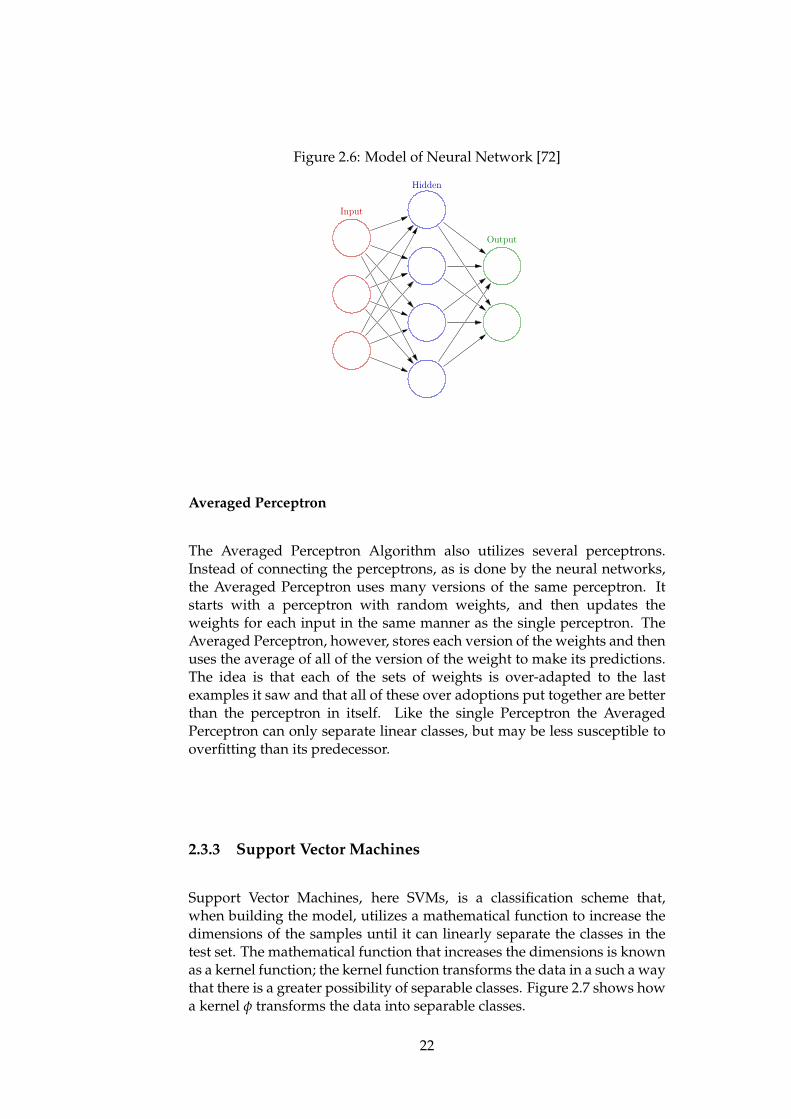
Figure 2.6: Model of Neural Network [72]

Averaged Perceptron

The Averaged Perceptron Algorithm also utilizes several perceptrons.Instead of connecting the perceptrons, as is done by the neural networks,the Averaged Perceptron uses many versions of the same perceptron. Itstarts with a perceptron with random weights, and then updates theweights for each input in the same manner as the single perceptron. TheAveraged Perceptron, however, stores each version of the weights and thenuses the average of all of the version of the weight to make its predictions.The idea is that each of the sets of weights is over-adapted to the lastexamples it saw and that all of these over adoptions put together are betterthan the perceptron in itself. Like the single Perceptron the AveragedPerceptron can only separate linear classes, but may be less susceptible tooverfitting than its predecessor.

2.3.3 Support Vector Machines

Support Vector Machines, here SVMs, is a classification scheme that,when building the model, utilizes a mathematical function to increase thedimensions of the samples until it can linearly separate the classes in thetest set. The mathematical function that increases the dimensions is knownas a kernel function; the kernel function transforms the data in a such a waythat there is a greater possibility of separable classes. Figure 2.7 shows howa kernel φ transforms the data into separable classes.

22

Figure 2.7: Model of an SVM’s Kernel [73]

When the SVM has reached a state where it can linearly separate theclasses, it attempts to find the optimal separation. The optimal separationis when the separator is equally far from the closest sample in each class,as shown in figure 2.8. When the SVM has built its model, it can predicton new data by performing the same kernel transformation on the newdata and subsequently observe what class it should belong to. SVMs areknown for working well on reasonably sized sample sets, but have poorerperformance on large sets [51]. SVMs can use both linear and non-linearkernel functions.

Figure 2.8: Model of optimal separation [73]

Pegasos Linear

An extension of the standard SVM, is the Pegasos Linear SVM. Thealgorithm optimizes the standard SVM, the method alternates betweenstochastic gradient descent steps and projection step to optimize the kernel[64].

Locally Deep

Another Extension of the SVM is the locally deep SVM. The algorithmspeeds up SVMs with non-linear kernel functions prediction while main-taining classification accuracy above an acceptable limit [45]. The algorithm

23

uses multiple kernels. It aims to learn a different kernel, hence classifier, foreach point in feature space.

2.3.4 Bayes Point Machine

Like the SVMs the Bayes Point Machine also utilizes a kernel function.Instead of finding a dimension where there is linear separability andusing only this decision boundary, the Bayes Point Machine attempts toseparate the classes in several dimensions, and stores each attemptedseparator. Subsequently it approximates a Bayes-Optimal, or minimalerror, intersection of the attempted separators and utilize it to make itspredictions. The intersection is a midpoint of the region and bisects thespace into two halves of equal volume and is known as the Bayes point.[42]

2.3.5 Logistic Regression

Logistic Regression is, despite its name, not a regression algorithmbut a binary classifier. The model estimates probability of a binaryoutcome based on some features. It works by measuring the relationshipof the variables and estimates probabilities using a cumulative logisticdistribution. The model is fast to train, but is limited to linear models.

2.3.6 Ensemble Learning

Ensemble Learning utilizes multiple learning algorithms to obtain betterpredictive powers. The idea behind is that several heads think better thanone. A common feature of machine learning problems is that it is im-possible to obtain perfect classifiers, which opens up the possibility that dif-ferent algorithms, with different biases, strengths and weaknesses togetheryield better results than a single learner. The learners are trained inde-pendently and predictions are combined in some way to make the overallprediction. There are several ways of combining the independent learnersand ensuring that they do not yield predictions that are too similar to eachother.

Perhaps the most common algorithm for ensemble learning is knownas Boosting. Boosting incrementally builds the ensemble model by trainingeach new model instance to emphasize samples were the previous modelsmiss-classified [36].

Bagging or Bootstrap aggregating, often abbreviated bagging, usesmultiple learners that have equal weight in the ensemble committee. Vari-ance is achieved by training each model on a randomly drawn subset of thedata [18].

Stacking trains several different machine learning algorithms on allof the available data and then uses a combiner algorithm that is trainedto make a final prediction using both the predictions from the and the

24

available data. Any machine learning algorithm may be used as acombiner, however, single-layer logistic regression is commonly used. [74]Stacking is at times referred to as meta ensemble learners [30] and will bereferred to as this in the thesis, just to separate standard machine learningalgorithms from stacked algorithms.

Decision Trees

Decision Trees are not Ensemble Learners by their self, but serve as the basisfor several ensemble learning algorithms. The Decision Tree is a structuresimilar to flowcharts, where each node contains a test on a feature, eachbranch represents the outcome of the test, and every end node contains aclass label. An example classifying the chance of survival on the Titanicis shown in figure 2.9. When decision trees are used as a classificationalgorithm, trees are built by splitting the data set into subsets based onthe outcomes regarding a feature and create corresponding sub trees. Thisis performed until each derived subtree leads to an end node.

Figure 2.9: Model of a decision tree [71]

Decision Forest

The Decision Forest is an algorithm that ensembles decision trees. Itcreates a multitude of decision trees and the output is the mode of thepredictions of the individual trees. It may use several of the ensembletechniques presented, but does most commonly utilize bagging for therandom selection of features to construct different decision trees. [61]

Decision Jungle

The Decision Jungle is a modification of the Decision Forest. Instead ofallowing only one path to every node in the trees, the Decision Jungleallows for a several paths from the root node to the end nodes. Thischanges the structure of the trees and complicates the learning process, butdoes, however, allow the trees to be smaller and consume less memory

25

and computational power, while also outperforming the Decision Jungle insome cases. The class is found by using directed acyclic graph search. [65]

2.3.7 FastTree

FastTree is yet another extension of the Decision Forest. What differsthe FastTree from the aforementioned algorithms is that it uses a nearestneighbor’s scheme to reduce the length of the individual trees. It is, asthe name suggests, a faster implementation of the Decision Forest, but incertain cases it performs better than the Decision Forest [58].

2.4 Predicting the stock market

As covered, the stock markets are influenced and moved by probablycountless factors. Finding out which factors are the most significant isthe first of several monumental challenges. By including too many factorsfor prediction, one is bound to find correlations, but unfortunately notcausation. The topic of this is covered in DJ Leinwebers article StupidData Miner Tricks, Overfitting the S&P 500 [48], where the author shows thatthe stock market S&P 500 were nearly perfectly correlated with the sheeppopulation and butter production in Bangladesh for over 10 years.As previously covered, we know that there are a lot of factors contributingto a stocks pricing. We also know that the factors that effect the stockmarket continuously change, leaving a predictor of a stock market in anawkward situation. By including too many factors for the prediction,we are bound do find correlations without causation. By includingtoo few factors for the prediction, we may not be able to predict themarket sufficiently well. Adding to an already difficult problem is theever changing nature of stock markets makes predicting them even morechallenging.

2.4.1 State of the art

There are vast numbers of papers and articles about the subject of stockmarket prediction using Machine Learning. Researcher from Japan havefound that that when comparing machine learning algorithms usingweekly data on Japanese stock market NIKKEI 225, a SVM outperformedits competitors [44]. The paper used several of the machine learning al-gorithms presented here, such as Neural Network and Decision Forest, butfound that integrating SVM with the other classification methods made itthe top performer. The fact that their combining model outperforms theother prediction (forecasting) methods gives hope for this thesis’ ensemblelearning approach to prediction of stock markets, as ensemble learningmethods works by combining machine learning algorithms.

Perhaps the most comprehensive research paper concerning stock mar-ket prediction with machine learning algorithms is the paper Surveying

26

stock market forecasting techniques – Part II: Soft computing methods by GS At-salakis. The paper surveys more than 100 research papers related to usingneural networks and other algorithms for stock market prediction and com-pares the different approaches. The paper concludes that the neural net-works has had the highest performance of the machine learning algorithms.But the paper also shows that there are several problems with selecting theappropriate amount of nodes and layers for the neural networks [5].

Ensemble Learning methods have also been attempted and researchedfor stock market prediction. It has been shown that ensemble learningtechniques may represent the stock indices behavior accurately [22].

The research on predicting the stock market with machine learningis somewhat schizophrenic. Some papers state that SVM is the optimalalgorithm, while other claim the Neural Network is the best choice andothers claim Ensemble Learning Models will outperform them all. Thismight be an indication that different machine learning algorithms willperform differently on different stock markets and with different inputs,exemplifying the No free lunch theorem, and indicating that results yieldedon the Norwegian stock market with a certain set of inputs might not berepresentative for other stock markets and inputs. It will however still beinteresting whether results found in the experiments will support previousfindings, which may imply whether these differences are caused by thebehavior of different stock markets, the choice of input for the learners orthe learners themselves.

27

28

Chapter 3

Methodology

29

This chapter describes how the results were obtained. Section 3.1gives a brief overview of the test environment. Section 3.2 describesand rationalizes the selection of the data used in the experiments. Italso explains the preprocessing of the data. Section 3.3 describes theimplementation of the algorithms. Section 3.4 outline how to understandthe results and the performance measures. Finally, section 3.5 discusses thelimitations of the thesis.

3.1 Test Environment

The aim of the tests carried out for this thesis were to:

Train a selection of two-class ensemble learning algorithms to predict daily stockmovement, and compare their performance to each other and non-ensemble ma-chine learning algorithms.

First, stock prediction was made into a two-class prediction problem.This was done by breaking the problem down to whether or not a stockwould rise with more than a threshold in N days. After some preliminarytesting, a decision was made to use the threshold of 0.05% predicting 1 day,more on the preliminary tests in 3.2.1, making the problem into a true/falsequestion for the machine learning algorithms:

Based on the knowledge we have today, what is the probability that a stock willrise with more than 0.05% by end of the day tomorrow.

The machine learning algorithms were trained using a selection of datathat is further discussed in 3.2.1 using data from 5.10.2011 to 30.09.2014,and attempted to predict the daily movements in the period from 1.10.2014to 1.7.2015.

Simply training and testing the algorithms on one or a few stocks wouldbe an unfair way to evaluate the performance of the algorithms, as stocksmay increase or decrease vastly in value in the test period, creating biases.Therefore, nearly all the stocks in OBX were included in testing to avoidbiased results.

37 machine learning algorithms and ensemble learning schemes weretrained on 22 stocks and their performance evaluated by Accuracy,Precision, Recall, F-Score and a simple Profit estimate. All tests werecarried out for every one of the 22 stocks and the mean, median andquartiles of the results are discussed in the results chapter.

3.1.1 Implementation Notes

Implementing Machine Learning Algorithm is time consuming, prone toerrors and notoriously difficult to optimize. To streamline the machine

30

learning process, Microsoft Azure Machine Learning© [24] environment andthe enclosed Machine Learning Algorithms were used for every algorithm.The environment performs all computations in an auto scaling cloudenvironment which makes it ideal for computational heavy modelling suchas ensemble learning. Using only one environment and no other externallibraries or self-made algorithms made the process efficient and less proneto errors and mistakes. The Algorithm modules are covered in details in3.3. All data preprocessing was done by using Python and R scripts, thatare further described in 3.2.2, with the exception of cross-validating whichused Microsoft Azure Machine Learning© built in module.

3.2 Data

3.2.1 Selection

What and why

As discussed in chapter 2, choosing data for building a model to predictthe stock market might be an impossible task. There are countless papers,theses and books written on the subject, and experts seemingly cannotagree upon what an optimal set of data could consist of. There is seem-ingly no viable way to safeguard the data selection from omitted variablebias discussed in section 2.1.9. Efforts were made in this thesis to choosedata that represented the Norwegian stock market as a whole, and also de-tailed information about the stocks that the machine learning algorithmswere to predict. The indices from the G20 stock exchanges were also in-cluded, as they give a good representation of the world economic as anentirety. Currency rates were included, as it holds valuable informationon how the Norwegian economy is doing compared to other economies.Lastly the Brent Oil price was included, as many Norwegian stocks on theOSE are highly dependent on the oil business.

It may be argued using this much data could lead to overfitting andfindings of correlation without causation. However, other will argue thatnot enough information was included. Data such as macroeconomic dataor interest rates is needed to make a valid model of any stock movement.The selection of data is an attempted compromise between too much andtoo little data, and can surely be criticized both for including and excludingtoo much data. The stocks in the OBX index, which consists of the 25 mostliquid companies on the main index of the OSE, were included, with theexception Aker Solution, Marine Harvest and BW LPG. These companiesdid major restructuring during the time period (i.e. the companies weredivided into smaller parts, changed names and acquired or merged withother companies). And if they were to be included in the model, a seri-ous attempt of adjusting for the restructuring would have been necessary.Adjusting for such restructuring is worth a thesis in itself, therefore thesestocks were excluded for simplicity. The stocks included are shown in fig-ure 3.1

31

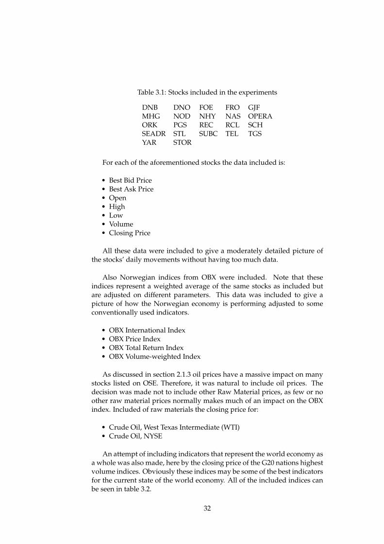
Table 3.1: Stocks included in the experiments

DNB DNO FOE FRO GJFMHG NOD NHY NAS OPERAORK PGS REC RCL SCHSEADR STL SUBC TEL TGSYAR STOR

For each of the aforementioned stocks the data included is:

• Best Bid Price• Best Ask Price• Open• High• Low• Volume• Closing Price

All these data were included to give a moderately detailed picture ofthe stocks’ daily movements without having too much data.

Also Norwegian indices from OBX were included. Note that theseindices represent a weighted average of the same stocks as included butare adjusted on different parameters. This data was included to give apicture of how the Norwegian economy is performing adjusted to someconventionally used indicators.

• OBX International Index• OBX Price Index• OBX Total Return Index• OBX Volume-weighted Index

As discussed in section 2.1.3 oil prices have a massive impact on manystocks listed on OSE. Therefore, it was natural to include oil prices. Thedecision was made not to include other Raw Material prices, as few or noother raw material prices normally makes much of an impact on the OBXindex. Included of raw materials the closing price for:

• Crude Oil, West Texas Intermediate (WTI)• Crude Oil, NYSE

An attempt of including indicators that represent the world economy asa whole was also made, here by the closing price of the G20 nations highestvolume indices. Obviously these indices may be some of the best indicatorsfor the current state of the world economy. All of the included indices canbe seen in table 3.2.

32

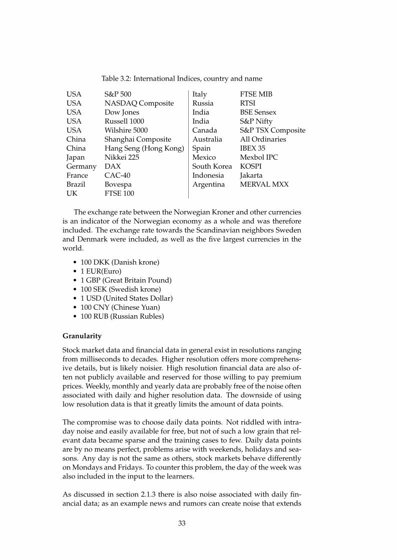
Table 3.2: International Indices, country and name

USA S&P 500 Italy FTSE MIBUSA NASDAQ Composite Russia RTSIUSA Dow Jones India BSE SensexUSA Russell 1000 India S&P NiftyUSA Wilshire 5000 Canada S&P TSX CompositeChina Shanghai Composite Australia All OrdinariesChina Hang Seng (Hong Kong) Spain IBEX 35Japan Nikkei 225 Mexico Mexbol IPCGermany DAX South Korea KOSPIFrance CAC-40 Indonesia JakartaBrazil Bovespa Argentina MERVAL MXXUK FTSE 100

The exchange rate between the Norwegian Kroner and other currenciesis an indicator of the Norwegian economy as a whole and was thereforeincluded. The exchange rate towards the Scandinavian neighbors Swedenand Denmark were included, as well as the five largest currencies in theworld.

• 100 DKK (Danish krone)• 1 EUR(Euro)• 1 GBP (Great Britain Pound)• 100 SEK (Swedish krone)• 1 USD (United States Dollar)• 100 CNY (Chinese Yuan)• 100 RUB (Russian Rubles)

Granularity

Stock market data and financial data in general exist in resolutions rangingfrom milliseconds to decades. Higher resolution offers more comprehens-ive details, but is likely noisier. High resolution financial data are also of-ten not publicly available and reserved for those willing to pay premiumprices. Weekly, monthly and yearly data are probably free of the noise oftenassociated with daily and higher resolution data. The downside of usinglow resolution data is that it greatly limits the amount of data points.

The compromise was to choose daily data points. Not riddled with intra-day noise and easily available for free, but not of such a low grain that rel-evant data became sparse and the training cases to few. Daily data pointsare by no means perfect, problems arise with weekends, holidays and sea-sons. Any day is not the same as others, stock markets behave differentlyon Mondays and Fridays. To counter this problem, the day of the week wasalso included in the input to the learners.

As discussed in section 2.1.3 there is also noise associated with daily fin-ancial data; as an example news and rumors can create noise that extends

33

beyond intra-day and affects closing prices but are quickly adjusted for thenext day.

Time Period

After settling on a daily resolution, the time period of the test data neededto be set. As discussed in chapter 2 using too old data could make themodel include outdated information. On the other hand, not havingenough data would make it impossible for the machine learners to createan adequately good model for prediction. The financial crisis of 2008 sentOBX down 54.1%. The market adjusted itself and in 2009 the index went upby 68.6% and in 2010 the it went up by 15.67 % up, making the movementsin these years highly abnormal. To avoid these abnormal years, data wasgathered from 06.10.2011 and to the day of the first experiments for thisthesis 01.07.2015, making it a total of 934 days of stock data to train and testthe learning algorithms.

Preliminary Tests

There are numerous ways of training a machine learning algorithm. One ofthe important decisions was to set the time line for the prediction, meaninghow many days of data that were used to predict how many days forward.If we were to use 3 days of data to predict 1 day ahead, that would meanthat if the current day was a Thursday, data from Tuesday, Wednesday andThursday would be used to predict the stocks movement on Friday. Asimple way of deciding these parameters was to perform some early testsand use the results to set the parameters. Due to time constraints, the pre-liminary test could not be performed on every stock. These preliminarytests were performed with Schibsted (SCH), which was chosen at random.

The results for the test with regard to the number of days of data touse in the prediction are laid out in table 3.3. 5 days of data yielded thehighest profit and precision, which, as is discussed in section 3.4.1, maybe regarded as the best indicator of performance for the problem at hand.For that simple reason, 5 days of data were used as input to the learners.More on how the data is structured using 5 days of data as input in section3.2.2. In the background the curse of dimensionality was discussed. Thesepreliminary results shows that more data, meaning here more days of data,yielded better results till 5 days of data. This indicates that the Curse ofDimensionality problem is, for the problem at hand, less influential thanthe need several days of data, meaning a great number of features. Thechoice was therefore taken to not focus on feature selection, but ratherattempting a broad range of machine learning algorithms.

34

Table 3.3: Preliminary results of days included for input

Days Profit Accuracy Precision Recall F-Score1 0.97978 0.582782 0.434879 0.218911 0.2471083 1.04782 0.580695 0.385825 0.179732 0.2102325 1.076791 0.588917 0.445489 0.186265 0.23287710 1.024078 0.583774 0.369036 0.197351 0.223694

The next preliminary test was to test how many days ahead to predict.The most instinctive idea is to predict the next day. It would however befoolish to assume that this is the optimal way without any testing. So thetest was performed and the average of all the learners are shown in table3.4. Predicting 1 day ahead yielded better results in every category than 2days ahead. As the results for predicting 2 days ahead were worse in everyway it was decided that further tests would likely produce even worseresults. This is an interesting result as it is an early indication that thereis some relationship between the stock movements and the data from theprevious day, and it implies that the stocks movement may be, in somedegree, predictable.

Table 3.4: Preliminary results of days forward to predict

Days Ahead Profit Accuracy Precision Recall F-Score1 1.076791 0.588917 0.445489 0.186265 0.2328772 1.004696 0.586374 0.412599 0.112971 0.177375

The final preliminary test that was carried out was to set the thresholdfor the two classes, meaning how much a stock needs to increase in valuebefore it is considered a positive. The results of the preliminary tests areshown in 3.5. Both 0.05% and 0% would generate convincing results.Notice that in the histograms in the figures 3.3, 3.2, 3.1, above 0% changehas the most even distribution, and the other histograms have a ratheruneven distribution of positives and negatives. Even distributions aregenerally considered better for machine learning, as uneven can createbiases. However, perhaps the most interesting result is whether or notit is plausible to derive a profit from the predictions, and therefore thefinal choice of threshold was to set it at 0.5%, as it seemingly has a largerpossibility of yielding a profit.

Table 3.5: Preliminary results of different threseholds

Threshold Profit Accuracy Precision Recall F-Score0 0.962631 0.54036 0.554905 0.595143 0.5552640.05 1.076791 0.588917 0.460851 0.192688 0.2328770.1 1.019174 0.719808 0.292927 0.073342 0.10494

35

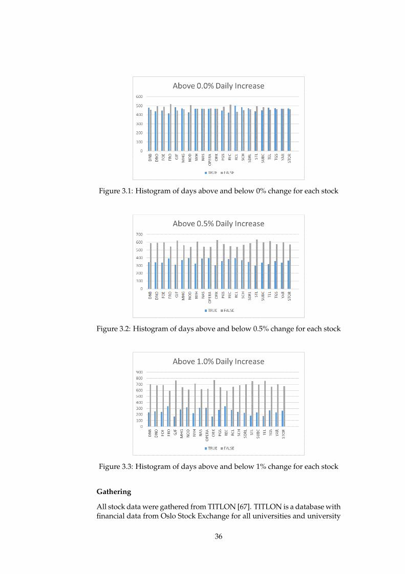
Figure 3.1: Histogram of days above and below 0% change for each stock

Figure 3.2: Histogram of days above and below 0.5% change for each stock

Figure 3.3: Histogram of days above and below 1% change for each stock

Gathering

All stock data were gathered from TITLON [67]. TITLON is a database withfinancial data from Oslo Stock Exchange for all universities and university

36

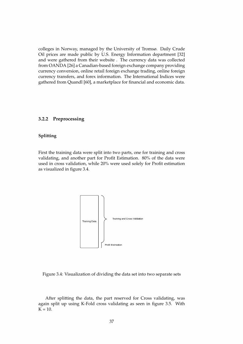
colleges in Norway, managed by the University of Tromsø. Daily CrudeOil prices are made public by U.S. Energy Information department [32]and were gathered from their website . The currency data was collectedfrom OANDA [26] a Canadian-based foreign exchange company providingcurrency conversion, online retail foreign exchange trading, online foreigncurrency transfers, and forex information. The International Indices weregathered from Quandl [60], a marketplace for financial and economic data.

3.2.2 Preprocessing

Splitting

First the training data were split into two parts, one for training and crossvalidating, and another part for Profit Estimation. 80% of the data wereused in cross validation, while 20% were used solely for Profit estimationas visualized in figure 3.4.

Figure 3.4: Visualization of dividing the data set into two separate sets

After splitting the data, the part reserved for Cross validating, wasagain split up using K-Fold cross validating as seen in figure 3.5. WithK = 10.

37

Figure 3.5: Visualization of k-fold cross validation

All of the stand-alone Machine Learning algorithms were trained onthe k folds of the training set and the results were evaluated with thetarget data to get True Positives, False Positives, True Negatives and FalseNegatives and Scored Probabilities. The Mean of all the folds are used tocalculate Accuracy, Precision, Recall and F-Score. Leading us to the nextgroup of the learners. The cross validation was performed by Azure MLsCross validation module

Time Series

As stocks prices may move in patterns, and are affected by changeshappening not only the previous day, but may be affected by changeshappening several days ago, simply including data from the previousday may not be sufficient to adequately predict a stock. To counter thisproblem several days of data were included as input for the learners. Afterpreliminary testing presented in section 3.2.1 the decision was made to use5 days of data as input, increasing the dimensionality of the input from 187to 936.

38

Looking at Change

The data was initially prepared as an array of all the data for each day.However, for data such as Best Bid Price, Best Ask Price, Open, High, Lowand Closing Prices for each stocks, currencies and indices, the importantinformation for a machine learning predictor does not lie in the real value.The data that should be included is the change from one point in theto another. Therefore, the real values were not fed to the learners, butrather the change between the days. This was calculated with equation3.1. Volume (i.e. numbers of stock traded that day) and the day of the weekwas the only indicator that was fed to the algorithms as real values and notas the change from the previous day.

new− oldold

= change (3.1)

Normalization

As discussed in section 2.2.9, in order to optimize the machine learningprocess, data should always be preprocessed in a way to avoid biases fromanomalies in the data. Normalization can be thought of as an adjustment ofvalues to a common scale, removing the disproportionate force of outliers.Z-Score is one of the more common ways of normalizing data, and waschosen for this thesis. Z-Score is a statistical measurement of a data pointrelationship with the mean of all the data. This method was chosen becauseit preserves range, i.e. minimum and maximum, and introduce dispersionof the data set, making it possible to see whether or not a data point istypical or atypical for the data set. Azure Machine Learning’s Normalizemodule was used, where each data point is calculated by:

Z =X− µ

σ(3.2)

where Z is the standard score, X is the real value, µ is the mean of thedataset and σ is the standard deviation of the dataset

Missing Data

With the choice of using financial data from several countries some prob-lems concerning incomplete data arose. There are different holidays in dif-ferent countries, meaning that the stock exchange is closed on certain daysin different countries. American Stock Exchanges are for example not openon the US Independence Day the 4th of July, while the Norwegian StockExchange is open for business this day. Also all stock exchanges are closedon weekends, while the Forex Market, where currencies are traded, is openevery day of the year.

Missing data need to be handled for optimal Machine Learning. Sincethe object of this thesis is to predict stocks listed on the Norwegian StockExchange the choice was made to use OBX as the reference, meaning that

39

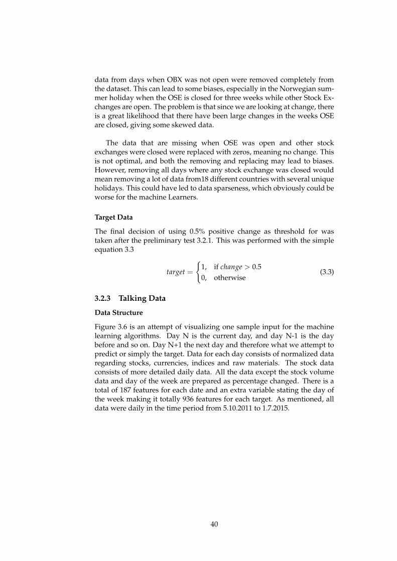
data from days when OBX was not open were removed completely fromthe dataset. This can lead to some biases, especially in the Norwegian sum-mer holiday when the OSE is closed for three weeks while other Stock Ex-changes are open. The problem is that since we are looking at change, thereis a great likelihood that there have been large changes in the weeks OSEare closed, giving some skewed data.

The data that are missing when OSE was open and other stockexchanges were closed were replaced with zeros, meaning no change. Thisis not optimal, and both the removing and replacing may lead to biases.However, removing all days where any stock exchange was closed wouldmean removing a lot of data from18 different countries with several uniqueholidays. This could have led to data sparseness, which obviously could beworse for the machine Learners.

Target Data

The final decision of using 0.5% positive change as threshold for wastaken after the preliminary test 3.2.1. This was performed with the simpleequation 3.3

target =

{1, if change > 0.50, otherwise

(3.3)

3.2.3 Talking Data

Data Structure

Figure 3.6 is an attempt of visualizing one sample input for the machinelearning algorithms. Day N is the current day, and day N-1 is the daybefore and so on. Day N+1 the next day and therefore what we attempt topredict or simply the target. Data for each day consists of normalized dataregarding stocks, currencies, indices and raw materials. The stock dataconsists of more detailed daily data. All the data except the stock volumedata and day of the week are prepared as percentage changed. There is atotal of 187 features for each date and an extra variable stating the day ofthe week making it totally 936 features for each target. As mentioned, alldata were daily in the time period from 5.10.2011 to 1.7.2015.

40

Figure 3.6: Visualization of how the data was made to a time series

Market Trends

When using historical financial data, it is important to note that in mosttime periods there is generally an upward trend, as most stock markets riseover time. This is also the case for the time period the training data coversin this thesis.

This is, however, a problem for anyone attempting to predict stocks,as sudden shocks in the stock market do occur. There is no such shock inthe training data, and therefore any model built with the training data isunlikely to be able to predict such a shock as the financial crisis of 2008.The period after the financial crisis in 2008 is biasedly prone towards anupward trend because there has been worldwide governmental subsidies,bail out packages and low interest rates and other efforts to stimulate eco-nomic growth. To understand what the learners should be able to predict,what they are unlikely to predict and what kind of biases they are likely tohave, we will have to do some analysis of the training data and the test data.

Since the dataset was divided into one part for testing and another partfor training, the datasets need to be reviewed both as a whole and each testset individually to better understand the results.

World Economy

There are many ways to review how the world economy was behaving inthe time period of the training data. First let us look at the trends at NYSE,the world’s largest stock exchange, which could to some degree reflect theworld economy as an entirety. Figure 3.7, shows the movements of NYSEthrough both the training and test period, the vertical line represent theseparation of the sets. As we can see from the figure, NYSE has an upward

41

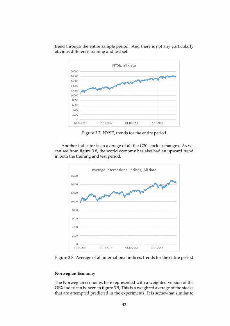
trend through the entire sample period. And there is not any particularlyobvious difference training and test set.

Figure 3.7: NYSE, trends for the entire period

Another indicator is an average of all the G20 stock exchanges. As wecan see from figure 3.8, the world economy has also had an upward trendin both the training and test period.

Figure 3.8: Average of all international indices, trends for the entire period

Norwegian Economy

The Norwegian economy, here represented with a weighted version of theOBX index can be seen in figure 3.9, This is a weighted average of the stocksthat are attempted predicted in the experiments. It is somewhat similar to

42

that of the world economy, a general upward trend. There are however twodips in the test period, which may negatively influence the results.

Figure 3.9: OBX weighted, trends for the entire period

When using indicators from foreign economies, comparing the Norwe-gian economy to foreign economies can be important. Inspecting the Nor-wegian currency against other may give insight into the movement of thestocks listed on the Norwegian stock market, and can be seen in figure 3.10.We can observe that the Norwegian krone has a particular weak period inthe test period, and that nearly all of the other currencies increased in valueagainst NOK in the test period.

Figure 3.10: NOK against all currencies, trends for the entire period

43

The Oil price movements in the can be observed in figure 3.11. The Oilprice plummeted to below half of its highest value in the training period.This may be the explentaion for the drop in NOK agianst other currencies,and why the Norwegian stock markets underperforms, to some extent, inthe test period.

Figure 3.11: Crude Oil per barrel, trends for the entire period

As a final review of the data included, we can observe that the worldeconomy was in an, perhaps unnatural, positive state through both thetraining and the test period, while the Norwegian economy was in a similarpositive state through the training period, but around the time when thetest period started, the Norwegian economy stagnated, likely due to thedropping oil price. Since this thesis attempts to predict Norwegian stocks,the fact that the test period is a period of low growth compared to the restof the world may influence the results negatively.

3.3 The Algorithms

3.3.1 How the modules work

The Azure Machine Learning modules work by connecting a model, likeTwo-Class Neural Network in figure 3.12 and data into a Cross-ValidateModel. After running what is shown in the algorithm, the cross-validatedmodel outputs two sets of data. The first data set is a list of scoredprobabilities for each input and the second set is performance measures.The performance measures are Accuracy, Precision, Recall and F-Score,

44

which are further discussed in 3.4.1. The machine learning model that isbuilt can be stored and be used for other input.

Figure 3.12: How a machine learning algorithm is trained in AzureMachine Learning Studio

3.3.2 Machine Learning Groups

As mentioned, 37 machine learning algorithms were tested. The algorithmsare in this thesis divided into three subgroups:

Standalone

First there is what will from now be called the Standalone Machine Learn-ing Algorithms. These are the “normal” machine learning algorithmsfound in Azure Machine Learning, and also in many other libraries. Theyare in this thesis called standalone algorithms to separate them fromstacked or meta machine learning algorithms. For the purpose of com-paring Ensemble Learners, the standalone algorithms are divided into twosubgroups.

• Non-Ensemble Learners:• Binary Neural Network (short training)• Binary Neural Network (long training)• Logistic Regression• Locally Deep Support Vector Machine• Bayes Point Machine• Averaged Perceptron• Support Vector Machine

• Ensemble Learners:• Decision Jungle• Fast Tree• Decision Forest

45

Figure 3.13: Illustration of N Standalone Learners, and how they werecross-validated

These algorithms were fed the training data and were cross-validatedas shown in 3.13 and later tested on the test set.

Simple Ensemble Learners

Using only predictions of other algorithms and simple criterias, sevenensemble schemes were created. These are henceforward called simpleensemble learners. These algorithms draws inspiration bagging ensemblelearners, and uses the output, i.e. the scored probabilities, and theirperformance measures, i.e. the Accuracy, Precision, Recall and F-Score,from the standalone learners to make its predictions. The seven schemeswere created after some simple preliminary testing. They work by waitingfor the standalone machine learning algorithms to finish, and afterwardsapply a criteria to the combined output to make its prediction as shown in3.14. The criterias used are shown in list 3.3.2.

• Criterias:• Majority Voting, i.e. over half the learners predicted class 1• Average Above > 0.5, the mean of the scored probabilities was above

0.5• Recall * Scored Probability > 0.3 for any of the learners• Accuracy * Scored Probability > 0.3 for any of the learners• F-Score * Scored Probability > 0.3 for any of the learners• Precision * Scored Probability > 0.3 for any of the learners• Any Above > 0.9 any one of the learners had a scored probability

above 0.9

46

Figure 3.14: Illustration of a single simple ensemble learner

Meta Ensemble Learners

Drawing inspiration from stacked machine learning algorithms, al-gorithms from now called Meta Ensemble Learners have been cre-ated. They work similarly to stacked machine learning algorithms,meaning that they utilize the predictions of other machine learningalgorithms as features for their predictions. They are called Metalearners in this thesis, to separate them from the more commonstacked machine learning algorithms utilizing a logistic regressionas its combiner. The same algorithms that have been tested as stan-dalone learners have been tested using this meta scheme. These canbe divided into two subgroups.

The first is The minimal meta ensemble learner. The implementationof these learners uses exclusively the scored probabilities from thestandalone learners as their input data. As shown in figure 3.15, thesealgorithms wait till the completion of every standalone algorithm.Then the algorithm uses the output from the standalone algorithmsas its input for learning. The same algorithms that were used for thestandalone were used for this minimalistic ensemble learner.

47

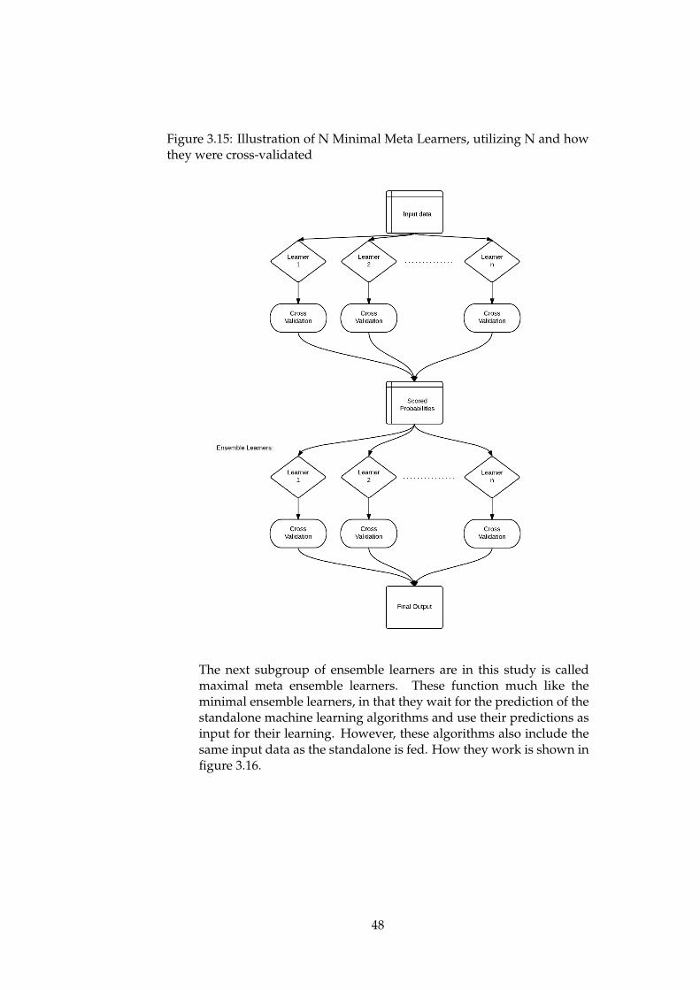
Figure 3.15: Illustration of N Minimal Meta Learners, utilizing N and howthey were cross-validated

The next subgroup of ensemble learners are in this study is calledmaximal meta ensemble learners. These function much like theminimal ensemble learners, in that they wait for the prediction of thestandalone machine learning algorithms and use their predictions asinput for their learning. However, these algorithms also include thesame input data as the standalone is fed. How they work is shown infigure 3.16.

48

Figure 3.16: Illustration of the maximal meta ensemble learners

Both of the meta ensemble learning schemes were tested with thesame algorithms as the standalone, giving us 20 algorithms; 10 forminimal and 10 for maximal. After all the algorithms were trainedand evaluated with Accuracy, Precision, Recall and F-Score, a profitestimate was calculated using unseen data.

3.3.3 Tuning Parameters

One of the limitations of this thesis is that the parameters of thealgorithms were not fine-tuned or optimized. The parameters weresimply set to the default value set by Azure Machine Learning Studio,with the exception of the random seed variable which was set to 0 sothat it can be replicated and the neural network which was trainedwith both 100 and 1000 number of learning iterations. A table of allthe possible parameters to tune is included in the appendix 5.1.

49

3.4 Understanding the results

3.4.1 Performance Measure

In binary classification, some of the most common performance meas-ures are, as we can recall from section 2.2.5, Precision, Accuracy, Re-call and F-Score. These are statistical measures that are calculatedfrom the number of true/false positive and negative. For the prob-lem in this thesis, a true positive would be when the learner correctlypredicted that a stock would rise with more than 0.05% the next day.False positive would be that the learner incorrectly predicted that thestock would rise. On the other hand, a true negative means that thelearner predicted correctly that the stock would not rise, and a falsenegative means that it predicted incorrectly that the stock would notrise.

If anyone were to trade stock based on the prediction of a binary pre-dictor, it would likely be wise to use an algorithm that rarely pre-dicted a false positive, since a false positive would cause the traderto buy a stock and lose money. For that reason, it may be argued thatprecision is the best measure, as it is a measure of the ratio betweentrue positives and false positives, or in other words, the ratio of howmany times the learner would make a profit compared to how manytimes the learner would create a loss, meaning that it would minimizethe risk of losing money. Because of this, the learner with the highestprecision may very well be the best if one wants to make a profit.This would especially be true in bearish periods when the market isnot expected to rise.

No risk, no reward. A common phrase in the financial world and inbullish market situations when stocks are expected to rise, higher riskstrategies may very well be the most lucrative. Recall measures theratio of how often the learner correctly predicts that a stock will riseagainst the number of times it fails or predict that the stock will rise.The higher the recall, the more often the learner will identify growthand thereby profit.

It is easy in retrospect to determine if a period was bullish or bear-ish, it is however more difficult to know what kind of period it is atthe moment. For that very reason both recall and precision may bean inadequate measure as they fail to tell the full story. The F-Scoreconsiders both Precision and Recall and is therefore more informativethan either of them by themselves. It is calculated by using the har-monic mean of the two values. The learner with the highest F-Scoreis therefore likely to do pretty well in periods that are bearish, bullishand anywhere in between.

Accuracy is also a more informative measure than precision and re-

50

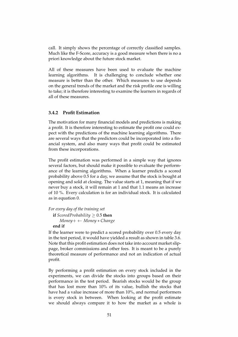
call. It simply shows the percentage of correctly classified samples.Much like the F-Score, accuracy is a good measure when there is no apriori knowledge about the future stock market.

All of these measures have been used to evaluate the machinelearning algorithms. It is challenging to conclude whether onemeasure is better than the other. Which measures to use dependson the general trends of the market and the risk profile one is willingto take; it is therefore interesting to examine the learners in regards ofall of these measures.

3.4.2 Profit Estimation

The motivation for many financial models and predictions is makinga profit. It is therefore interesting to estimate the profit one could ex-pect with the predictions of the machine learning algorithms. Thereare several ways that the predictors could be incorporated into a fin-ancial system, and also many ways that profit could be estimatedfrom these incorporations.

The profit estimation was performed in a simple way that ignoresseveral factors, but should make it possible to evaluate the perform-ance of the learning algorithms. When a learner predicts a scoredprobability above 0.5 for a day, we assume that the stock is bought atopening and sold at closing. The value starts at 1, meaning that if wenever buy a stock, it will remain at 1 and that 1.1 means an increaseof 10 %. Every calculation is for an individual stock. It is calculatedas in equation 0.

For every day of the training setif ScoredProbability ≥ 0.5 then

Money+← Money ∗ Changeend if

If the learner were to predict a scored probability over 0.5 every dayin the test period, it would have yielded a result as shown in table 3.6.Note that this profit estimation does not take into account market slip-page, broker commissions and other fees. It is meant to be a purelytheoretical measure of performance and not an indication of actualprofit.

By performing a profit estimation on every stock included in theexperiments, we can divide the stocks into groups based on theirperformance in the test period. Bearish stocks would be the groupthat has lost more than 10% of its value, bullish the stocks thathave had a value increase of more than 10%, and normal performersis every stock in between. When looking at the profit estimatewe should always compare it to how the market as a whole is

51

performing. Therefore, the average profit estimate is an importantmeasure that will work as a baseline for many of the results.

Table 3.6: Profit estimate for owning the stock through the entire test period

Stock: Profit EsimateAverage 1.07FOE 0.46SDRL 0.46SCH 0.74OPER 0.77STL 0.78SUBC 0.83NYH 0.92GJF 0.93STOR 0.94DNO 1.00MHG 1.01PGS 1.01ORK 1.07DNB 1.09TGS 1.11TEL 1.22YAR 1.27NOD 1.45RCL 1.46NAS 1.46FRO 2.51

3.4.3 Statistical significance

The Mann-Whitney U Test has been used for deciding whether thereare significant differences between the results yielded for the differentmachines learning algorithms and the groups of algorithms. It maybe used as a measure, since the assumption of the Mann-Whitney UTest is that there is independence within the sample set and mutualindependence, which is true for the independently trained machinelearning algorithms used in the experiments.There are issues with using Mann-Whitney U Test finding outwhether or not there are statistical differences between pairs of theresults. The Mann-Whitney test is a ranked test that simply showswhether it is likely that two data sets are from different groups.However, it does not take into account that the machine learning al-gorithms in the experiments conducted are predicting the same stock;this may be an issue if some stocks are more easily predicted than oth-ers, as it may bias the results.

A solution to this issue could be to use Wilcoxon signed-rank test,

52

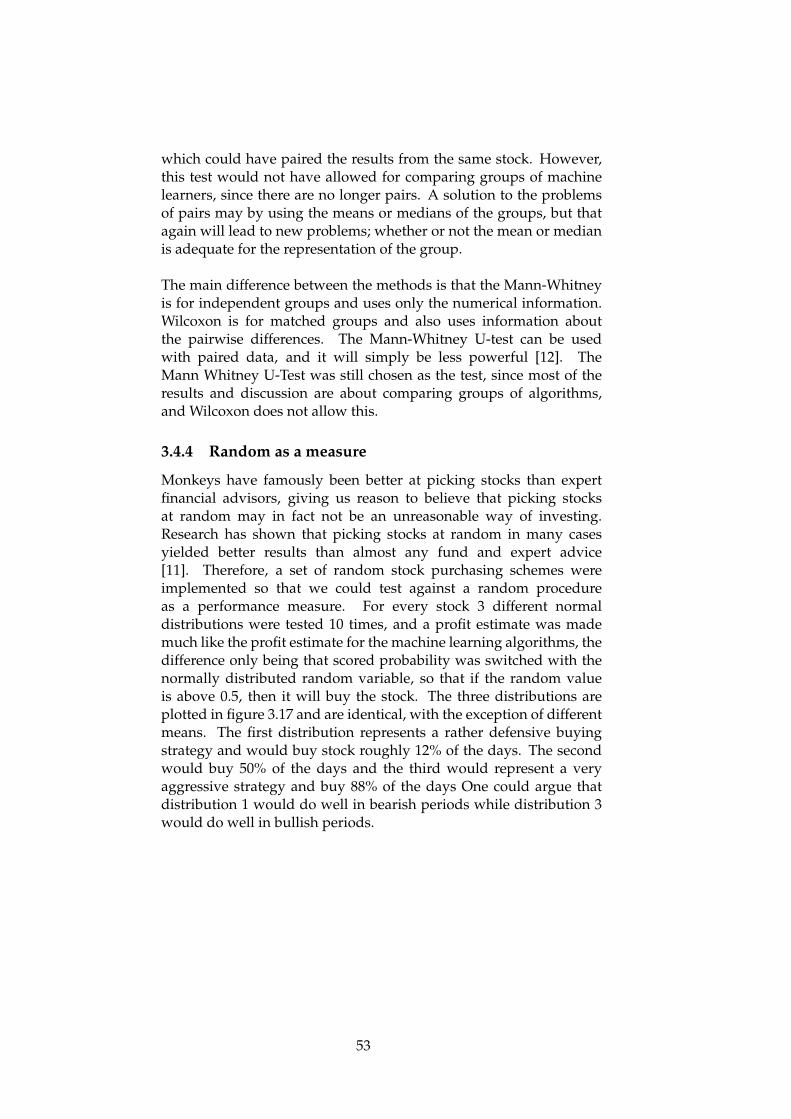
which could have paired the results from the same stock. However,this test would not have allowed for comparing groups of machinelearners, since there are no longer pairs. A solution to the problemsof pairs may by using the means or medians of the groups, but thatagain will lead to new problems; whether or not the mean or medianis adequate for the representation of the group.

The main difference between the methods is that the Mann-Whitneyis for independent groups and uses only the numerical information.Wilcoxon is for matched groups and also uses information aboutthe pairwise differences. The Mann-Whitney U-test can be usedwith paired data, and it will simply be less powerful [12]. TheMann Whitney U-Test was still chosen as the test, since most of theresults and discussion are about comparing groups of algorithms,and Wilcoxon does not allow this.

3.4.4 Random as a measure

Monkeys have famously been better at picking stocks than expertfinancial advisors, giving us reason to believe that picking stocksat random may in fact not be an unreasonable way of investing.Research has shown that picking stocks at random in many casesyielded better results than almost any fund and expert advice[11]. Therefore, a set of random stock purchasing schemes wereimplemented so that we could test against a random procedureas a performance measure. For every stock 3 different normaldistributions were tested 10 times, and a profit estimate was mademuch like the profit estimate for the machine learning algorithms, thedifference only being that scored probability was switched with thenormally distributed random variable, so that if the random valueis above 0.5, then it will buy the stock. The three distributions areplotted in figure 3.17 and are identical, with the exception of differentmeans. The first distribution represents a rather defensive buyingstrategy and would buy stock roughly 12% of the days. The secondwould buy 50% of the days and the third would represent a veryaggressive strategy and buy 88% of the days One could argue thatdistribution 1 would do well in bearish periods while distribution 3would do well in bullish periods.

53

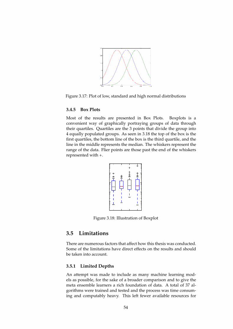
Figure 3.17: Plot of low, standard and high normal distributions

3.4.5 Box Plots

Most of the results are presented in Box Plots. Boxplots is aconvenient way of graphically portraying groups of data throughtheir quartiles. Quartiles are the 3 points that divide the group into4 equally populated groups. As seen in 3.18 the top of the box is thefirst quartiles, the bottom line of the box is the third quartile, and theline in the middle represents the median. The whiskers represent therange of the data. Flier points are those past the end of the whiskersrepresented with +.

Figure 3.18: Illustration of Boxplot

3.5 Limitations

There are numerous factors that affect how this thesis was conducted.Some of the limitations have direct effects on the results and shouldbe taken into account.

3.5.1 Limited Depths

An attempt was made to include as many machine learning mod-els as possible, for the sake of a broader comparison and to give themeta ensemble learners a rich foundation of data. A total of 37 al-gorithms were trained and tested and the process was time consum-ing and computably heavy. This left fewer available resources for

54

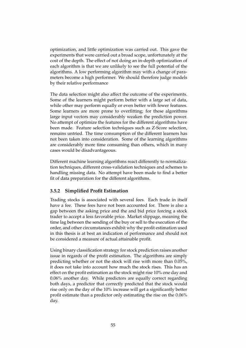
optimization, and little optimization was carried out. This gave theexperiments that were carried out a broad scope, unfortunately at thecost of the depth. The effect of not doing an in-depth optimization ofeach algorithm is that we are unlikely to see the full potential of thealgorithms. A low performing algorithm may with a change of para-meters become a high performer. We should therefore judge modelsby their relative performance

The data selection might also affect the outcome of the experiments.Some of the learners might perform better with a large set of data,while other may perform equally or even better with fewer features.Some learners are more prone to overfitting; for these algorithmslarge input vectors may considerably weaken the prediction power.No attempt of optimize the features for the different algorithms havebeen made. Feature selection techniques such as Z-Score selection,remains untried. The time consumption of the different learners hasnot been taken into consideration. Some of the learning algorithmsare considerably more time consuming than others, which in manycases would be disadvantageous.

Different machine learning algorithms react differently to normaliza-tion techniques, different cross-validation techniques and schemes tohandling missing data. No attempt have been made to find a betterfit of data preparation for the different algorithms.

3.5.2 Simplified Profit Estimation

Trading stocks is associated with several fees. Each trade in itselfhave a fee. These fees have not been accounted for. There is also agap between the asking price and the and bid price forcing a stocktrader to accept a less favorable price. Market slippage, meaning thetime lag between the sending of the buy or sell to the execution of theorder, and other circumstances exhibit why the profit estimation usedin this thesis is at best an indication of performance and should notbe considered a measure of actual attainable profit.

Using binary classification strategy for stock prediction raises anotherissue in regards of the profit estimation. The algorithms are simplypredicting whether or not the stock will rise with more than 0.05%,it does not take into account how much the stock rises. This has aneffect on the profit estimation as the stock might rise 10% one day and0.06% another day. While predictors are equally correct regardingboth days, a predictor that correctly predicted that the stock wouldrise only on the day of the 10% increase will get a significantly betterprofit estimate than a predictor only estimating the rise on the 0.06%day.

55

56

Chapter 4

Experiments

57

This chapter describes the results gathered from the experiments.Section 4.1 describes how to read the results. Section 4.2 presentsthe results. Section 4.3 reflects upon and analyze the results andcompares the performance of the machine learning algorithms.

4.1 How to read the result

4.1.1 Diversity and Adjustments

Normally when one is evaluating machine learning algorithms it iscommon to use a combination of statistical measures and real life per-formance. The same approach has been used in this thesis. However,profit estimation, which is a type of real life performance, has beenemphasized. It is emphasized because like with most applicationsof machine learning, there is a great desire to have machine learningthat can be applied to actual problems.

One of the main reasons that the statistical measures are used is be-cause real life performance measures are riddled with noise and onecan easily be fooled by the dumb luck of a machine learning al-gorithm. This thesis mostly uses profit estimation, and can do sobecause it analyses the mean of 23 different stock for each learner,severely decreasing the likelihood of chance influencing the results.We know that examining profit estimate of the single machine learn-ing algorithms predictions is not especially interesting as it is prone tobiases and chance and may not reveal anything about the algorithmsactual prediction power.

In order to make sure that the results are valid within reasonabledoubt, Mann-Whitney U tests have been performed on the differentresults, and a table has been made which shows whether two batchesof results can with a significance level of 99.95% certainty distinguishthat the two results are inherently different and that there is a signi-ficant difference between the sets of results. The tables are laid out sothat the intersection between two algorithms or groups of algorithmsrepresents whether there is a significant difference between the twogroups of profit estimates. When the p-value is over 0.05, it meansthat we cannot be more than 95% sure that the results are not the res-ult of noisy data and luck, and these intersections are marked witha capitalized N for No. When the p-value is above 0.05 and there issignificance it is marked with a capitalized Y for Yes in the table. Thereal P-Values were not included as a measure for readability.

Simply inspecting the real values of the profit yielded has signific-ant downsides, as the performance of the stock in the test period to ahigh degree influences the result. To separate the performance of themachine learning algorithm from the performance of the stock and

58

the market in general, all of the results are presented adjusted to thedevelopment of entire stock market (OBX). The market adjustmentmeans that every profit estimate is subtracted by the profit estimateof owning an OBX index fund through the test period. What thismeans is that while a learner before the adjustment would have madea profit if its value was above 1. After the adjustment it means thatprofit is at above 1.0-1.07 = -0.07 and that performing better than themarket is above 0.

4.1.2 Categorizing the stocks

In addition to inspecting all the stocks at the same time, the stockshave been categorized by their overall performance throughout thetest period. The stocks have been divided into three groups BearStocks, Bull Stocks and Normal Stocks as shown in 4.1. The criteria forwhich category the stock is assigned to is simply whether the stockhas increased or decreased with more than 10%, or as we see moreformally in equation 4.1

Category =

Bull Stocks, if change > 0.1Bear Stocks, if change < −0.1Normal Stocks, otherwise

(4.1)

The categories shown in table 4.1, named All Stocks, Bull Stocks andBear stocks are grouped together in different plots. The top figureshows the results for all the stocks, the second from the top showsthe same profit estimations but only regarding the Bear Stocks and thebottom plot shows profit estimates for Bull Stocks. Normal Stocks plotsof these were however not included as they were very similar to theAll Stocks plots, and may have made the presentation of the resultstoo chaotic. Also the performance of the Normal Stocks can be derivedfrom the other results as All Stocks is of course the sum of Bull Stocks,Bear Stocks and Normal Stocks.

The reason for including the plots of the Bull and Bear stocks is that itcan tell us how the learners act and predict and whether the learnersproduce defensive or aggressive purchasing strategies. But the per-haps most important insight it gives, is how the algorithms wouldhandle time periods unlike the test period, for example how the pre-dictions would be in very bearish markets. As we remember fromsection 3.2.3 the test period is a quite normal period, with a slightupward trend, but unfortunately the stock market does not alwaysact in this way. By looking exclusively at the Bear Stocks it may givevaluable insight into how the learner would act in a crash and theBull Stocks plots gives into how the learner would handle a stock rally.This renders some more certainty in answering a research question onwhether it is possible to make a profit, particularly in a long term set-

59

Table 4.1: Categorized by Profit Estimation, Bull, Bear and Normal stocks

Bear Stocks Normal Stocks Bear StocksFOE 0.457203 NYH 0.916528 TGS 1.10581SDRL 0.457342 GJF 0.930831 TEL 1.221986SCH 0.738532 STOR 0.935403 YAR 1.274334OPER 0.770428 DNO 1.002643 NOD 1.451187STL 0.785388 MHG 1.00723 RCL 1.461378SUBC 0.827248 PGS 1.008354 NAS 1.461401

ORK 1.070568 FRO 2.506716DNB 1.088113

ting when both crashes and rallies are bound to occur, and is thereforeimportant in the question of whether it is possible to make a profit ornot.

To further understand how the bull and bear stocks should beviewed, we have to look at what is good for a Bull Stock. Remem-ber that the average of all the stocks is 1.07 and that adjusted for themarket it is obviously 0. Since all of the bull stocks outperform themarket as a whole we would expect more of a profit as well. In fact,by simply owning any of the bull stocks throughout the test periodwe are guaranteed 1.1 - 1.07 = 0.03 above the market. But further scru-tinizing the Bear Stocks we can observe that the mean of all the bullstocks is 0.427, meaning that we should expect results in this regionfor high performing algorithms. It is the other way around for theBear Stocks; by owning any of the stocks throughout the period oneis guaranteed a loss of at least -0.17 and the mean of the bear stocksadjusted for the market is -0.397, and the results should be inspectedwith this in mind.

4.1.3 Results Overview

The results that are included, are included as an attempt of answeringthe research questions posed in this thesis, and a small justification isincluded for every plot. Most of the results are shown as box plotswith an additional mark for the mean. As we recall from section3.4.5 the box indicates the quartiles, the line the median and it cantell us something about the entirety of the results. All of the resultsone learner have from every stock are always presented together.Mean is perhaps the most important measure in the box plot for usto look at, as it shows the results of what we could expect to gainif we were to distribute our money equally for the single learner forevery stock. This would likely be the most reasonable investmentstrategy, and is therefore highlighted. The median tells us how largea part of the stocks it is likely to make a profit if we follow the singlelearner’s prediction. The box tells us what we could expect for 50% of

60

the stocks and the whiskers and outliers show the extremes that onepossibly could encounter if you were to put all your money into onestock.It is important to note that in this chapter the machine learningalgorithm types, meaning the standalone learners, minimal andmaximal meta ensemble learners, simple ensemble learners arereferred to as the machine learning types or most often groups.Algorithms such as Neural Network, Pegasos-Linear SVM, DecisionJungle and so on are referred to as algorithms. The results are dividedinto different sections. First there is an overview of the profit estimatefor every machine learning algorithm tested on every stock is shownin the first figure 4.1. Later on in the result section, we furtherexamine each group of learners by themselves. Let us take a quickrecap of the groups and algorithms presented in chapter 3 and then anoverview of all the results presented in section 4.2.In table 4.2 we canobserve all the algorithms tested, as we know the same 9 algorithmsare tested for both the Meta Ensemble Learners and as Standalonealgorithms, and that the so called Simple Ensemble Learners uses 7different schemes to make predictions.

Table 4.2: Algorithms

Meta EnsembleStandalone Simple Ensemble

Maximal MinimalNeural Network Accuracy

Locally Deep SVM PrecisionLogistic Regression Sum Above

Decision Forest F-ScoreDecision Jungle Any Above

FastTree RecallBayes Point Machine PrecisionAveraged PerceptronPegasos Linear SVM

61

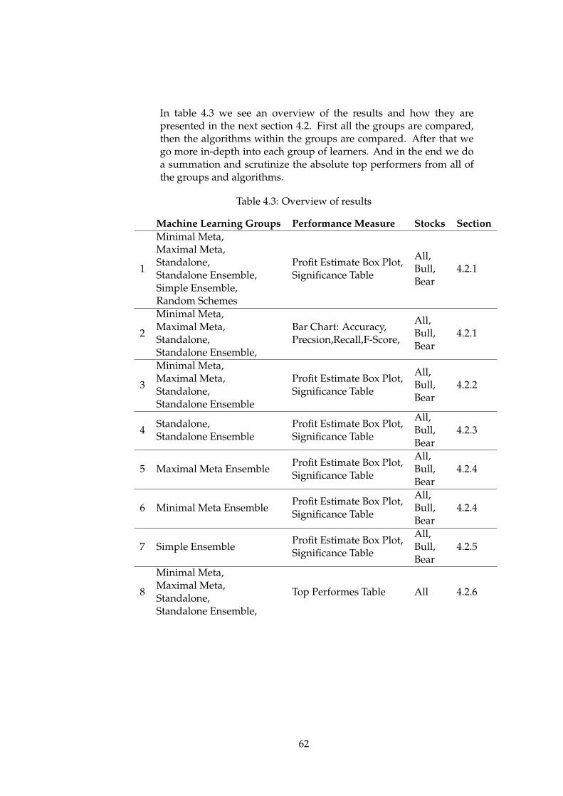
In table 4.3 we see an overview of the results and how they arepresented in the next section 4.2. First all the groups are compared,then the algorithms within the groups are compared. After that wego more in-depth into each group of learners. And in the end we doa summation and scrutinize the absolute top performers from all ofthe groups and algorithms.

Table 4.3: Overview of results

Machine Learning Groups Performance Measure Stocks Section

1

Minimal Meta,Maximal Meta,Standalone,Standalone Ensemble,Simple Ensemble,Random Schemes

Profit Estimate Box Plot,Significance Table

All,Bull,Bear

4.2.1

2

Minimal Meta,Maximal Meta,Standalone,Standalone Ensemble,

Bar Chart: Accuracy,Precsion,Recall,F-Score,

All,Bull,Bear

4.2.1

3

Minimal Meta,Maximal Meta,Standalone,Standalone Ensemble

Profit Estimate Box Plot,Significance Table

All,Bull,Bear

4.2.2

4Standalone,Standalone Ensemble

Profit Estimate Box Plot,Significance Table

All,Bull,Bear

4.2.3

5 Maximal Meta EnsembleProfit Estimate Box Plot,Significance Table

All,Bull,Bear

4.2.4

6 Minimal Meta EnsembleProfit Estimate Box Plot,Significance Table

All,Bull,Bear

4.2.4

7 Simple EnsembleProfit Estimate Box Plot,Significance Table

All,Bull,Bear

4.2.5

8

Minimal Meta,Maximal Meta,Standalone,Standalone Ensemble,

Top Performes Table All 4.2.6

62

4.2 Results

4.2.1 Groups Compared

The first results are laid out in 4.1; these results are shown to answerthis thesis’ hypothesis. The figure is a compact summary of the profitestimates of all the tested algorithms. It shows whether one couldexpect to make a profit from any of the types of algorithms. It alsoshows the difference between the groups of algorithms, and whetherthe meta ensemble learners gained from their additional input. Thegroups of algorithms are plotted together, meaning that for examplethe Maximal Meta Ensemble, the Neural Network, Decision Jungleand so on are included in the group. The profit estimates for eachone can in the plot be compared with the others and the random dis-tributions. Each data point represents the profit estimate of a singlelearner’s result on a single stock. As an example the one point is FastTree for the Minimal Meta Ensemble type for SCH. Table 4.4 showswhich of the results plotted in 4.1 that are significant.

Let us inspect figure 4.1 All Stocks first. One can observe that three ofthe algorithm groups, namely Standalone, Maximal Meta Ensembleand Standalone Ensemble learners, have a mean that is slightly betterthan the market. Observing the p-value table we can see that just inone case we may say with significance that these algorithms outper-form the market represented here at 0 by OBX. It is however not bymuch, only 0.06 or 0.6% more profit than OBX, a meager result forthe algorithm group with the highest mean, namely the Standalonelearners. We can however, not say with significance that the Stan-dalone algorithms outperform the Maximal Meta Ensemble Learnersor the Standalone Ensemble Learners. We can also observe that thestandalone learners have a bigger box, meaning that the distributionis sparser and that the variation within the group is quite large.

After that we see that the random purchasing schemes have a meanlower than OBX, but have both the highest and lowest performersof all the algorithms and schemes. The mean is also, perhaps sur-prisingly, not much lower than the other algorithms and OBX. TheSimple Ensemble Learners and the Minimal Meta Ensemble Learnersperform poorer than OBX and significantly poorer than the other ma-chine learning methods.

When observing 4.4 Bull Stocks and Bear Stocks one immediately no-tices that the random purchasing schemes vary much more in per-formance on bull and bear stocks than the learners. The simple en-semble learners also have a greater variation in performance than theother machine learning types. That random purchasing is more in-fluenced by the performance of the stock than the other schemes isnot very surprising, and it can be seen as a strength of the machine

63

learning algorithms that they do not perform badly when used onBear Stocks.

In the Bull Stocks plot, the means are generally higher than in the AllStocks plot. This comes as no surprise as it is easier to make a profit onrising stocks. What it is more of a surprise is that only the standalonealgorithms and the simple ensemble learners have a mean above 0.1.From 2.1.10 we separated the stocks into groups that made a profitlarger than 10%. Owning any of these stocks guaranteed a result ofat least 0.03 owning an equal share of all of these stocks would yielda 0.43 profit above OBX. All of the machine learners and schemesperform below the average results of the stocks. This is an indica-tion that they were to defensive in their purchasing strategy. As wecan see the random purchasing strategies perform notably best forthe Bull Stocks, and best of them all the Random High strategy, whichpurchases stocks the most often. This can be seen as yet another indic-ation that the learners did not properly manage to separate the bullstocks from the other stocks and purchase these at a higher frequency.

On the other hand we can see that for the Bear Stocks there is, yet againquite unsurprisingly, an opposite reaction. There is in general lessprofit yielded, and there is not much difference between the learners,but the random stocks perform notably poorer. It is impressivethat the all of the learners with the exception of the Simple Learnersmanaged to yield a profit larger than OBX.

Table 4.4: Significance Table, Groups Compared

Max

imal

Meta

Ensem

ble

Min

imal

Meta

Ensem

ble

Standalo

ne

Standalo

ne Ensem

ble

Random

low

Random

center

ed

Random

high

OSX

Minimal Meta Ensemble YStandalone N Y

Standalone Ensemble N Y NRandom low Y Y Y Y

Random centered Y Y Y Y NRandom high Y Y Y Y N N

OSX Y Y Y Y Y Y YSimple Ensemble Y Y Y Y Y Y Y Y

64

Figure 4.1: Groups Compared

65

To further investigate the difference in the groups of machine learn-ing algorithms, this section scrutinizes their precision, accuracy andrecall and F-Score for the Minimal and Maximal Meta learners aswell as the standalone learners, including the standalone ensemblelearners. This is done as an attempt to see whether the meta ensemblelearners performed any better because of their extra input from othermachine learning algorithms, the top performers from the previousresults. The results can be seen in 4.2, where the bars represent themean and the whiskers the standard deviation. The first noticeableresults are that the Accuracy is fairly similar in both the mean andstandard deviation, although the maximal meta learners somewhatoutperform the others in this category for all the stock types. Whatmakes that result interesting is that, as we remember from the pre-vious sections, the standalone algorithms outperformed the maximalmeta learners regarding profit estimation. Adding to that, we canalso see that the maximal meta learners have a considerably higherprecision as well.

In section 3.4.1 we discussed the statistical measures, and made aseemingly intuitive assumption that a higher precision is better forBearish periods and higher Recall is better for Bullish periods fora stock market prediction problem, and that Accuracy and F-Scorewere good measures for the overall time periods. However, compar-ing the results in 4.2 regarding the Accuracy, Precision, Recall andF-Score for all the stocks, the Bearish stocks and the Bullish Stocks,it is hard to conclude that these assumptions were correct. The stan-dalone algorithms outperform the Maximal Meta algorithms in all ofthe profit measures, and it does so in a very similar manner for all thestock types. This also goes for the bearish and bullish stocks, eventhough the Maximal Meta Ensemble Learners have notably higherPrecision.

Why the profit measure and the statistical measures are showing dif-ferent top performers is hard to grasp. One of the main causes couldbe, as highlighted in the limitations section 3.5, that the performancemeasures have some quirks in that a correct classification counts asa single true positive/negative for the statistical measures, while forprofit estimates, it has a series of degrees that can change the result.It may seem that even though the Maximal Meta Learners classifymore correctly, the Standalone learners can make bigger profits orsmaller losses on each trade. The fact that the meta learners actuallyhave a higher Accuracy mean that these types of learners may not beany worse than the standalone learners. They may in fact be betterat other problems, and simply do not perform perfectly on this exactproblem. This is an indication that the Maximal Meta algorithms mayhave performed better with other thresholds or features.

The minimal meta ensemble learners did not perform very well

66

regarding the profit estimate, but hold up better for these statisticalmeasures. They have higher Accuracy than the standalone learnersfor All Stocks and Bear Stocks, and have a lower or similar precision,recall and F-Score, for all the other categories.

Figure 4.2: Statistical Measures, Groups Compared

4.2.2 Learners Compared

This section shows the results that allow us to compare the perform-ance of the different algorithms in each group of learners.

67

Comparing Machine Learning Algorithms

Here the results for all the machine learning algorithms are shown,in the same manner as in section 4.2.1, with All Stocks, Bull Stocks andBear Stocks adjusted for OSX in 4.3 and the p-values in 4.5. Theseresults are shown to see whether there are any differences betweenthe standard machine learning algorithms, and this gives us an ideaof how the algorithms compare to each other regardless of the inputprovided, before we in later sections can see the results of the ma-chine learning algorithms in regards of only one scheme at a time.With all the machine learning algorithms it means that for, for ex-ample Binary Neural Network, the results show the performance ofthe Neural Network as a standalone learner, as a Minimal Meta En-semble Learner and a Maximal Meta Ensemble Learner combined.

Six of the algorithms have a mean that is above 0, Locally Deep SVM,Decision Forrest, Decision Jungle, Averaged perceptron Pegasos-Linear SVM and the Fast Tree. Of all of them Averaged Perceptronand the Pegasos-Linear SVM have the highest means, but as seen inthe p-value table they are not significantly better than several of theother algorithms. The locally deep SVM also performs well, but notwell enough to prove that it is significantly better than most of theother algorithms. Logistic Regression performs by far the worst, butdoes so in a surprisingly steady way. This is due to the algorithm pro-ducing a very defensive purchasing scheme, meaning that it nearlynever purchased a stock.

The observations to take away from the Bull Stocks and Bear Stocksplots is that the Locally Deep SVM and the Decision Forest overper-form compared to the other stock on the Bull Stocks, and that the SVMperforms better than on the Bear Stocks than on the Bull Stocks, whichis certainly impressive for the Bear Stocks, but perhaps nearly equallyunimpressive for the Bull Stocks. The fact that none of the algorithmshave a mean that is far from zero is interesting. This result can gener-ally mean two things; first that the learners are actually able to makethe decision that the stock will fall in value and choose not to buy.This could be a sign of that the machine learning algorithms makesreasonable predictions. The other thing it could mean is that the al-gorithms simply choose to stay out of the market, i.e. not buy stocksvery often, and therefore stay close to zero, which in many cases isnot a bad choice, but if the algorithms do this often it all becomesquite meaningless.

Now that we have reviewed the results from the machine learningalgorithms, it is interesting to see whether the results from themachine learning types are similar to the results to the typescombined. This might give an indication whether one of thealgorithms is generally better at stock market prediction regardless of

68

inputs; whether some algorithms perform better with certain inputsor if it is perhaps simply luck that separate them. This follows in thenext sections.

Table 4.5: Significance Table, All Algorithms

Neura

l Network

Logistic

Regres

sion

Locally

Deep SV

M

Decisi

on Forest

Decisi

on Jungle

FastTr

ee

Bayes

Point M

achin

e

Averag

edPerc

eptro

n

Logistic Regression NLocally Deep SVM N Y

Decision Forest N Y NDecision Jungle N Y N N

FastTree N N N N NBayes Point Machine N Y N N N NAveraged Perceptron Y Y N N Y Y YPegasos Linear SVM Y Y N N Y Y Y N

69

Figure 4.3: All Algorithms Compared

70

4.2.3 Standalone

The figure 4.4 shows the standalone learners and the standalone en-semble learners compared to each other. These results are included togive the reader an idea of the performance of the different standardmachine learning algorithms with the standalone algorithms. Table4.2.3 shows the p values of significant differences for the same resultsas the plot. Note here that in the plot the Y axis is on a slightly dif-ferent scale than in the previous plots, and that the results may seemskewed when comparing the results here with figure 4.1.

Reviewing the plot, we are quickly able to see that see that the res-ults are not much different from what we saw in the previous sec-tion 4.2.2. The biggest difference for all stocks is that the FastTreealgorithms mean has fallen below 0 and that the locally deep SVMhas gained a meager profit. But other than that there is not much dif-ference. There is in fact a bigger and more noticeable difference ofwhat we can see with the naked eye in the P-Value table. The P-Valuetable shows that the results from the standalone learners may showthat our two top performing algorithms, the Pegasos Linear SVM andAveraged Perceptron, can be shown to have statistically significantdifferent result than the other algorithm except the Bayes Point Ma-chine and each other. This is a better result than we got for all of themachine learning algorithms. And the result comes despite having athird of the sample size. This may tell us that there is less variance inthe groups for the standalone learners alone than in the other types ofalgorithms. This is interesting because it shows in another way thatthere is in fact a difference between the groups of learners.

Table 4.6: Significance Table, Standalone Algorithms

Neura

l Network

Logistic

Regres

sion

Locally

Deep SV

M

Decisi

on Forest

Decisi

on Jungle

FastTr

ee

Bayes

Point M

achin

e

Averag

edPerc

eptro

n

Logistic Regression YLocally Deep SVM N Y

Decision Forest N Y NDecision Jungle N Y N N

FastTree N N N N NBayes Point Machine N Y N N N YAveraged Perceptron Y Y N N Y Y NPegasos Linear SVM Y Y Y Y Y Y N N

71

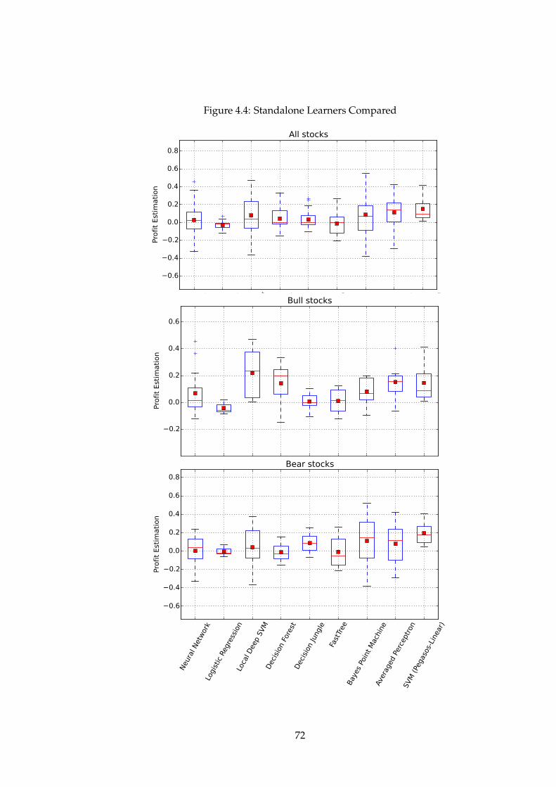
Figure 4.4: Standalone Learners Compared

72

4.2.4 Meta ensemble

Maximal

In figure 4.5 we see the results from the Minimal Meta EnsembleLearners, and their associated P-Values in table 4.2.4. These res-ults were included to show the performance of the different machinelearning algorithms compared with each other for the maximal metascheme. Examining the All Stocks plot, there are again small differ-ences between the learners, and nearly every algorithm has a meanabove 0. Bayes Point Machine and Logistic Regression have a meanbelow 0.

The Significance table shows that we with statistical significanceonly may say that over the top performers, yet again the PegasosLinear SVM and the Averaged Perceptron, are better than the lowestperformers. The locally Deep SVM and the Decision Forest performbetter in this scheme than in the standalone. For the Bull Stocks andBear Stocks, a lot of the results are similar to the standalone schemeand all of the learners in general. Locally Deep SVM and DecisionForest fluctuate the most between the stock types, a clear sign ofmore aggressive purchasing schemes. Another interesting takeawayfrom these results is that the Peagsos Linear SVM performs betterfor the Bear Stocks than with the Bull Stocks, which is highly unusualand counter intuitive. One may speculate on the reasons for thisresult; and it is likely due to a defensive strategy and very accurateprediction of the Bear Stocks.

Table 4.7: Significance Table, Maximal Meta Ensemble Algorithms

Neura

l Network

Logistic

Regres

sion

Locally

Deep SV

M

Decisi

on Forest

Decisi

on Jungle

FastTr

ee

Bayes

Point M

achin

e

Averag

edPerc

eptro

n

Logistic Regression NLocally Deep SVM N N

Decision Forest N Y NDecision Jungle N N N N

FastTree N N N N NBayes Point Machine N N N Y N NAveraged Perceptron Y Y N N Y N YPegasos Linear SVM N Y Y N N N Y N

73

Figure 4.5: Maximal Meta Ensemble Learners

74

Minimal

In figure 4.5 we see the results from the Maximal Meta EnsembleLearners, and their associated P-Values in table 4.2.4. These res-ults were included to show the performance of the different machinelearning algorithms compared with each other for the minimal metascheme. As we recall from the section 3.3.2, these algorithms get alot less input than the others, as its only input is the prediction fromthe standalone learners. We can recall from 4.1 that the minimal metaalgorithms performed poorer than the standalone algorithms and themaximal meta ensemble learners. This is also visible in the plot, aswe can see that the majority of the algorithms have a mean below 0,effectively meaning that an index fund is a better choice than usingthe algorithm.

What we see is small distributions, meaning that the results aresimilar for every stock. This is a strong indication that the predictorssimply too seldom predict a stock rise. This is seemingly a biggerproblem for these the minimal meta ensemble schemes than it isfor the maximal and standalone. There can be a twofold reason forthis: The scored probabilities given to the learning algorithms maysimply not give enough information for a meaningful prediction orthe scored probabilities from the other algorithms are biased closer to0, which is likely, as there are more days that the stocks do not risemore than 0.5%. For the Bull Stocks and Bear Stocks, the same patternoccurs as we have seen for the standalone and maximal algorithms.

Table 4.8: Significance Table, Minimal Meta Ensemble Algorithms

Neura

l Network

Logistic

Regres

sion

LocallY

Deep SV

M

Decisi

on Forest

Decisi

on Jungle

FastTr

ee

Bayes

Point M

achin

e

Averag

edPerc

eptro

n

Logistic Regression NLocallY Deep SVM N N

Decision Forest N N NDecision Jungle N N N N

FastTree N N N N NBayes Point Machine Y Y N N N NAveraged Perceptron Y N N N N N NPegasos Linear SVM N N N N N N N N

75

Figure 4.6: Minimal Meta Ensemble Learners Compared

76

4.2.5 Simple Ensemble

While some save the best for last, the poorest group of learners areto be displayed last here: The Simple Ensemble Learners. The resultsare shown in figure 4.7 and whether there is any significance in theresults is shown in table 4.9. These results were included to provideinsight into the different simple ensemble learners. The simple en-semble learners were perhaps given an unfair opportunity. Whilethe other algorithms have been optimized by years of research anda large Microsoft team, these learners had its parameters from a fewswift preliminary tests. The problem with this is best shown by thePrecision scheme, which nearly never bought any stocks, and defin-itely should have had a lower threshold for purchasing stocks.

If it as a trend that these simple ensemble schemes for purchasingstocks all had to high thresholds, they would likely perform decentlyfor Bearish stocks. However, one can observe from figure 4.1 andfigure 4.7, that this is in fact not the case. As we see, the precisionscheme outperforms the other schemes for the Bear Stocks by simplynot doing anything, which hardly is impressive.

Of the different simple ensemble schemes, only Sum Above and AnyAbove had a mean above 0. But all of the schemes perform relativelysimilar, and as we can observe in table 4.9,we can with statistical sig-nificance only say that Precision is the worst scheme. We can notstatistically separate the results due to the variance within the per-formances of the schemes on the different stocks, increasing the prob-ability that the results are in fact derived from chance.

Table 4.9: Significance Table, Simple Ensemble Learners

Accura

cy

Majo

rity

Sum

Above

F-Score

Any Above

FastTr

ee

Majority NSum Above N N

F-Score N N NAny Above N N N N

Recall N N N N NPrecision Y Y Y Y Y Y

77

Figure 4.7: Simple Ensemble Learners

78

4.2.6 Top Performers

The 15 overall top performers and their average profit estimate aboveOSX for all the stocks are shown in table 4.10. These results wereincluded as an attempt of a final summation of the results and toshow the potential of profit making. As we can observe, the top per-former is not unexpectedly the Pegasos Linear SVM from the stan-dalone group. It yields a profit of more than 10 % more than OBXover the test period. As we can remember from previous sections,the Pegasos Linear SVM has been one of the top performers for all ofthe machine learning groups. And we can also remember from sec-tion 4.2.1 that the standalone algorithms performed the best, so it isanything but shocking that it is one of the top performers. The Av-eraged Perceptron occupies the two next positions in the table, bothas a Standalone Learner and as a Maximal Meta Ensemble Learner,amplifying the belief that the Averaged Perceptron is an algorithmthat is well fit for stock market predictions. We can see that all the top10 performs are from either the Maximal Meta Ensemble Learners orthe Standalone Learners, giving us strong reason to believe that thesegroups are the best for the problem at hand.

Table 4.10: Top Performers

Profit Algorithm Group0.151 SVM (Pegasos-Linear) Standalone0.111 Averaged Perceptron Standalone0.087 Averaged Perceptron Maximal Meta Ensemble0.086 Bayes Point Machine Standalone0.078 Local Deep SVM (LDSVM) Standalone0.072 SVM (Pegasos-Linear) Maximal Meta Ensemble0.067 Decision Forest Maximal Meta Ensemble0.056 Local Deep SVM (LDSVM) Maximal Meta Ensemble0.042 Decision Forest Standalone0.033 Neural Network Maximal Meta Ensemble0.031 Decision Jungle Standalone0.027 Neural Network Standalone0.026 FastTree Maximal Meta Ensemble0.025 Decision Forest Minimal Meta Ensemble0.024 Local Deep SVM (LDSVM) Minimal Meta Ensemble

4.3 Analysis

4.3.1 Can you make a profit?

As discussed in the limitations section 3.5, there are several weak-nesses with the profit estimate posed in this thesis which makes adefinite conclusion to whether one could make a profit with a ma-

79

chine learning algorithm difficult to postulate. However, the res-ults show that a handful of the algorithms do indeed yield a profitgreater than the market, which has been the baseline for the res-ults. When comparing the groups against OSX and Random purchas-ing strategies in section 4.2.1, we observed that Maximal Meta En-semble Learners, Standalone and Standalone Ensemble learners out-performed the market with statistical significance. The significancegave reason to believe that there is a possibility of making a profit.

Trading Schemes

To reduce risk, it is common to disperse the money into differentstocks and sometimes also different purchasing schemes. This wouldbe wise to implement also for a machine learning implementation ofstock trading. As we can see from all of the plots in this thesis, some-times the algorithm performs very poorly, and by simply trading onestock with one algorithm, there is a big risk of losing most of yourmoney. There is of course also a chance of making a lot of money,but gambling strategies like this are not at all recommended and willlikely not hold up over time. One of the more sensible strategies formaking a profit would be to spread your money equally to each stockand stick to a strategy. However, the real life problem of fees im-perfects markets. Not being able to buy and sell at the wanted pricequickly enough, makes the strategy of dividing your money betweenall stocks available more of an implausible solution.

Top Performers

When observing the overall top performers, we can observe that theStandalone Pegasos Linear SVM beats the market by a staggering15%, which might be enough of a profit to outrun the fees. Notethat fees are normally set at a fixed price, therefore if we were totrade with large amounts of money, each trade would have a relat-ively lower price than if we trade with small amounts of money. Thefees also vary from broker to broker. On the other hand, it is harder tobuy and sell large amounts of stocks than small, and this may causesome loss of profit. But the 15% profit over the market yielded by thetop performer might very well have been profitable in actual trading.While we can with statistical significance claim that Standalone Pe-gasos Linear SVM outperforms the market from the first significancetable 4.4, we cannot say that it is better than the Standalone AveragedPerceptron or the Bayes Point Machine, and the extra profit might bederived from chance. On the other hand, we know from the same sig-nificance table that it is a better performer than the standalone Locallydeep SVM, and therefore we can say that it is likely that StandalonePegasos Linear SVM would yield a profit larger than the locally deep

80

SVM at 7.8%.

The test period

Whether over 7.8% from the profit estimate is enough to make a profitin the real world is as we know difficult to say, but let us for the sakeof argument assume that it would. There is also another issue regard-ing an adequate answer to whether we could expect a profit. Thetest period is as discussed in section 3.2.3 a generally positive timeperiod. As we know from history the market has its ups and downs,and it is likely that this test period does not adequately represent anyother time period. The Bull and Bear results were included to givebetter insight into how the predictors would work in crashes and ral-lies. We have observed in 4.1 and discussed in the talking data section3.2.3, how they perform surprisingly well for Bear stocks and surpris-ingly poor for Bull stocks. These results give us reason to believe thatthe learners, and especially the top performers yield reasonable res-ults even in crash-like scenarios and therefore rarely make a big loss.But we should not forget that there is no justification for choosingthis time period, and as we know, the world economy is in constantchange and not two periods of time are equal. We should therefore becareful claiming that one could have made a similar profit to the onesin these results in another time period. We should however not forgetthat the standalone Pegasos Linear SVM and the other top performersdid not simply make a profit, they outperformed the market substan-tially. The fact that they also handled the bear stock without losingmoney is a strong argument that the most fitting machine learningalgorithms would not perform badly even in downward markets.

Lady Luck

If 37 people spun the roulette wheel 22 times each, it is likely thatsome of them would make a profit. If 37 machine learning algorithmsattempts to predict 22 stocks, it is also likely that some of them wouldmake a profit, even if the stock market was entirely random. The factthat some out of many are bound to perform well, is another sign ofthat we should interpret any results regarding any prediction of anysystem with noise or general randomness with a pinch of salt. Onecould talk about probabilities, U test and distributions, but there willalways be that insecurity of chance. The results in this thesis are obvi-ously affected by this, however one could argue that the fact that thiswas not a single buy/sell transaction, but rather a series stretchingover nearly a year and hundreds of buy/sell decisions, that it is lessprone to luck. And by observing the results with the Whitney ManU test we observed that there was a difference between the profits ofall the random purchasing strategies and the best types. The fact that

81

we can say with 99.95% probability that the top performers are inher-ently different from the random strategies, gives us an argument thatthe results are very likely valid, and the chances of chance is playinga trick on us are low. But we should always keep in mind that theWhitney Mann U Test shows that the results are different, but thatdifferent is not necessarily better. A scheme that purchased a stockfor the first 50% of the days and remained inactive the last 50% of thedays would be different from a scheme that bought a random 50%of the days, and their profit estimates would likely be very different.On the other hand, we should not forget that all the experiments aredone with 22 stocks, and that this obviously decreases the chance ofluck being the main influencer of the result.

Theory bound models

Most of the researchers studying finance and the predictability ofthe stock market would criticize any machine learning model fordrawing conclusions not being based upon a theory. In finance andmost other social sciences the normal procedure is to first make ahypothesis upon why, for example, variable a effects variable b, andthen test the hypothesis using some statistical test and subsequentlydraw a conclusion upon whether or not variable a effects variableb. Machine Learning turns this around, as we skip the theory part.As an example one of the machine learning algorithms tested heremight through the data discover that when variable a increases by1% variable b increases by 2%, and use this in its predictions. Findingsuch correlations may seem great, but it may fool us into thinkingthat there is a direct cause and effect between variable a and b. Itmay very well be a third variable not included in the data set thataffects variable a, and a fourth variable effecting variable b. Sincewe obviously will never be able to include all possible data that mayaffect variable b, it leaves us in an awkward position. The machinelearning algorithm has no way of testing that there is cause and effectbetween a and b, and since it is not bound to any theory, there is noway of justifying the correlation. Because stocks can be affected bynear infinite variables, it is almost impossible to conclude without anydoubt whether one could make a profit over time or not. On the otherhand, one could argue that there is no need for the machine learningalgorithms to be able to explain a theory that it bases its predictionsupon. For a stock prediction problem, it may be enough to predictcorrectly 51%, or at whatever percentage it starts yielding a profit, ofthe time for it to be useful. This is illustrated by the top performersthat yielded a more than satisfactory profit on the test period.

82

Optimization

If one were to predict stock with machine learning algorithmswith actual money, the experiments performed here would likelyjust be a preliminary test to help aid the choice of one or a fewalgorithms that would be optimized further. There is a great dealof research regarding machine learning on real life problems wheregreat improvements have been made by manually adjusting theparameters of the algorithms. One could take it even further usingoptimization schemes such as genetic optimization. The machinelearning types and algorithms tested here have not been given theadvantage of such an enhancement, which certainly can be used asan argument that it is possible for the algorithms to improve theirperformance. As is pointed out in the limitations 3.5, the experimentshere were focused on a broader research trying many algorithmsrather than optimization of a single one.

Variable selection

An issue that occurs for any model based prediction is, as discussed inthe feature selection section 2.2.11, the input data or features. It is wellknown in machine learning that feature optimization can improvethe performance of a machine learning algorithm [38]. A problemlike stock prediction can be, as discussed in the forces that movesstocks section 2.1.3, particularly susceptible for omitted variable bias.Therefore, feature selection could very well have improved the resultspresented in this thesis. This thesis used quite a high number offeatures, which may lead to problems of finding correlations withoutcausation. One can actually observe from the results in this thesisthat more features is not necessarily better, as the Maximal EnsembleLearners get the same inputs as the standalone learners and someextra inputs, but fail to outperform them. On the other hand, byexcluding features, we risk not being able to predict certain thingsthat are being caused by external variables. No matter if one shouldhave included more variables or fewer, it is highly unlikely that thefeatures chosen for this thesis is the optimal set of features. Therefore,it is likely that one could get improved results with another setof features, an argument that it is possible for a machine learningalgorithm to yield even greater profits than what is shown here.

Risk and Reward

As we observed in the results there is a surprisingly small differencebetween the result on the bull and the bear stocks. Investigating therandom distributions purchasing strategies made it possible for uswith an even greater conviction to say that the algorithms tradedquite defensively. This theory of defensive predictions can be shownby observing the low recall in the plot in figure 4.2. The plot shows

83

that recall is lower than precision in every case, and as was discussedin 3.4.1 this means that the algorithms more often than not predictedthat the stock would not rise the next day. One can argue that this is apositive property of the learners as a trading scheme, as it will lowerthe risk, since fewer purchases provide a lower risk. That they aredefensive may be used as an argument that the picking a threshold of0.05% for the target of the machine learning algorithms was a gooddecision. The choice was made after it yielded the greatest profits inthe preliminary tests.

Regardless of how much risk one would want to take, and how manypurchases that are reasonable, it is clear that the algorithms did notpredict perfectly. This is easily observable in the plot in figure 4.2,where accuracy, precision, recall and F-Score are quite low for all ofthe learners. The unfulfilled potential is further illustrated by therandom schemes outperforming all of the other algorithms for thebear stocks. It presents an argument that the algorithms predicted toodefensively, and that they therefore made a much smaller profit thanpossible. These additional profits could have made it possible for usto say with more certainty whether one actually could have made aprofit using machine learning for the time period. The balancing actof finding the perfect ratio between risk and reward is strenuous. Itis doubtful that the thresholds set for the experiments were optimal,and quite certain that improvements can be made to both increase theprofit or decrease the risk.Another choice influencing both the risk and the performance wasthe choice of a daily resolution. The choice was taken for convenienceand because it might have shown interesting results. It may howevernot be the optimal resolution. As we can see from the results, thelearners, with the exception of a few, have not yielded particularlylarge profits compared to the risk taken. With another resolution thelearners may have performed better. Many of the automated tradingschemes used today purchase stocks with a much higher frequencythan daily purchases. On the other hand, longer term predictionsmay also have yielded interesting results with lower risk and perhapsalso larger profits.

Binary Classification

As discussed, changing the threshold of 0.05% may offer greater res-ults or less risk. This may lead us into the question of whether binaryclassification is the right choice for attempting to make a profit onthe stock market. On one hand one could argue that in the end any-thing regarding profit in the stock market boils down to one question:Should I own this stock? On the other hand, one may argue that thebinary result does not provide enough information to decide whetheron should purchase a stock or not. Multi-class classification couldprovide more information by utilizing classes richer in information,

84

classes that indicated how much it predicted the stock to rise or fall.This would also allow for trading scheme where one could weigh theamount of money spent on purchasing each stock. This is to some ex-tent possible with two-class classification; one could achieve similarperformances by changing the threshold of the outputs, and the trad-ing schemes could have been made by using the scored probabilities.This was to some extent attempted by using the so called simple en-semble learners, but they only looked at one stock at a time and there-fore fall short of any scheme looking at all the stocks at the same time.

There are however scenarios where two class classification fallsshort, namely with shorting and other more complicated ways oftrading stocks. Shorting is essentially betting that a stock will fall invalue, and makes it possible to make a profit by predicting a stock’sdecreasing value. Both Multi-Class classification and Regressionwould have allowed for predictions that would have allowed forshorting. Regression seems perfect for stock trading schemes that useboth buying and shorting stocks, as it shows the real value of what itpredicts. However, if you say: I will purchase a stock if the regressionpredicts a result above zero, and short the stock if it predicts belowzero, the problem is actually a two class problem, and would yieldthe same results as the tested algorithms only with a threshold at 0%change for the targets. One could set other thresholds on when to buy,when to sell and when to hold, but the essence of making the probleminto a regression problem is that at one point we would have to setthresholds of when to purchase, when to short and when to hold,which boils the problem down to a classification problem. Multi-classclassification would have allowed for these different categories, andmay therefore be the optimal way of predicting stock. However, byshorting and using more classes, we increase the risk and maybe alsothe error rate, as it makes the problem more complex. Errors can alsobe more expensive using a profit estimate, as shorting a rising stockresults in a loss.

Similar research

The results presented regarding whether one could make a profitin the stock market seem to coincide with the published paperson the topic. There is however a divide in the research, usuallydepending on the background of the paper authors. Papers wherethe authors view the stock market as a problem that can be solvedusing smart algorithms and historical data are usually from anArtificial Intelligence and Informatics background. These papersoften show that there is great promise in applying machine learningfor predicting stocks [47][20], and many show results of models thatcan yield profits. On the other hand, papers where the authors arefrom an economical background seem to emphasize to a much higherdegree the problems with predicting stocks using historical data [14]

85

. These economists have shown that it is not necessarily possible tosay that a test period is representative, and as previously covered,they have even shown that random strategies may perform as well asany other scheme given a long enough test period. There are someresearchers that from a Machine Learning background address theproblems of ever changing data, such as the stock market, on how todraw knowledge from the decisions boundaries, and problems withany time series data when using machine learning and data mining[77]. The results presented in this chapter also show that there arepossibilities, and it seems that one could in fact make a profit usingmachine learning on the stock market, but there are however somebasic underlying problems with prediction stocks one cannot escape.

4.3.2 Comparing Schemes and algorithms

Predicting with predictions

One of the sub goals of this thesis was to implement and test machinelearning algorithms that used the predictions of other machine learn-ing algorithms as part of its input. These schemes, called Minimaland Maximal Meta Ensemble and Simple Learners, and their resultshave been shown. The results may not seem too impressive at firstglance, but when one investigates and theorizes around their seem-ingly low performance, we might see why the methods should notbe dropped as a research topic, and that further research is needed toconclusively draw conclusions.

Let us first compare the results of the types of algorithms in figure4.1 the Standalone learners and Maximal Meta Ensemble Learners,since they were the top performers. We could through the WhitneyMann U test separate the results from these types, and show that theyyielded better results than the other types of algorithms. Betweenthese two top performing groups there were however not a statist-ical difference in the results. We can therefore say that the experi-ments produced no evidence supporting the statement that the ma-chine learning algorithms got an improved performance by havingpredictions of other algorithms as an input. There are however alsono statistical significant evidence showing that the maximal meta en-semble learners performed any poorer. Therefore, we cannot excludethe chance of the standalone schemes running into a stretch of luck.We can see in the top performer section 4.2.6, that the standalonealgorithms in general perform better than their Maximal Meta En-semble counterparts, but there are a few exceptions. The DecisionForest, FastTree and Neural Network all performed better for theMaximal Meta Ensemble Learner than the standalone. These res-ults might give reason to believe that some algorithms could benefitmore from the additional input than others. It is however challen-ging to grasp why some algorithms perform better with the different

86

schemes.

An interesting observation made in section 4.2.1 where we investig-ated the results of the different types using statistical measures, is thateven though the Maximal Meta Ensemble Learners outperformed thestandalone algorithms in all of the statistical measures, it did not yieldhigher profits. This not only shows that the limitations of the profit es-timates as well as the limitations of the statistical measures, but it alsoleaves more room for the discussion on whether the Maximal MetaEnsemble Learners may in fact outperform the standalone algorithmson other problems or sets of data, as they did predict correctly morethan the standalone learners. And we must also not forget that theStandalone algorithms have gained from being optimized in a muchhigher degree than the Maximal Meta Learners, as they come de-fault with carefully set parameters. One of the issues that may causethe Maximal Meta Learners not to perform better than its standalonecounterpart is that there is a high number of features, in fact over 900.This may cause the predictions from the other algorithms to drown,showing yet another reason that these types of algorithms need tobe further researched before one can say with certainty whether theyproduce better results than standalone algorithms or not.

When comparing the statistical measures of the Minimal Meta En-semble learner with the others, we can observe that the results are notas poor as the profit estimate would suggest. As an example the min-imal meta has higher accuracy than the standalone learners. Whenlooking deeper into the reason why the Minimal Meta Learners per-formed as poorly as they did in profit estimate, we see that the recallof the Minimal Meta Learners is quite a bit lower than for the otherstrategies. This shows that the algorithms predicted that the stockwould not rise the next day almost every day, which actually couldbe considered a decent strategy, since it is true for more days thannot. These findings show that the Minimal Meta Ensemble Learnersmay have benefited more than the other types by a different thresholdthat created a more equal distribution between the true/false. Onthe other hand, the Minimal Meta Ensemble Scheme might not getenough information to make a good prediction the way they havebeen tested in this thesis. It is highly likely that its input from othermachine learning algorithms predictions are too similar to each other,and that they therefore fail to make adequately good predictions. Theschemes could be further researched by drawing inspiration fromother Ensemble Learning schemes differentiating the input to the ma-chine learning algorithms. The Maximal Meta Ensemble Learnersmight also benefit from changes that lead to a more differentiatedinput.

The so-called Simple Ensemble Learners consisted of 7 differentsimple schemes of using the output from other machine learning al-

87

gorithms to make predictions. The inspirations of the schemes camefrom other Ensemble Learners, the Averaged Perceptron and com-monly used Majority Voting. The results that these schemes yieldedwere however less than impressive, and did in general perform a lotpoorer than its counterparts. When we investigate into why theyperformed so poorly, we can see that all of the schemes performedpoorly, and that there was no particularly bright star among them.They did in general perform below average, and we can say withthe support of the Whitney Mann U test, that the results were poorerthan the other types. It is unlikely that the schemes Majority and SumAbove are simply bad schemes that will never work, as similar imple-mentations exist in for example Averaged Perceptron and Bayes PointMachine as we can recall from section 2.3.2. What is more likely isthat these were optimized very poorly, and that different thresholdsshould have been set. As we discussed with the minimal meta en-semble learner, these learners may also gain from having a more dif-ferentiated input. The other schemes using the statistical measuresF-Score, Precision, Accuracy and Recall did not manage to convinceanyone with their performance, but yet again this could be due to badparameters and thresholds.

The Algorithms

One of the research questions presented in this thesis whether or notthe algorithms would perform differently. Given the random natureof the stock market, a different performance of the algorithms was notgiven. We have however shown that there is a significant differencebetween some of the algorithms tested in this thesis. Even though weonce again should be careful drawing explicit conclusions, becausethe test set might not be representative for any other test period, wecan say with some conviction that there was a difference in perform-ance.

It is also interesting to investigate the performance of the differentalgorithms to find out which ones are the most suited for stock pre-diction and why. The first thing we observed in section 4.2.2 was thatthere were surprisingly small differences between the performance ofthe algorithms, and even though the Whitney Mann U Test showeda significant difference between some of the algorithms, the majoritywere in fact without significant difference. The reason for the smalldifferences might very well be the random nature of the stock mar-ket, and perhaps we cannot conclude that all the algorithms performdifferently, and that only some of them might have different results.

When comparing the algorithms to each other we noticed that therewere meager differences between the top performers. And manyof the differences where not significant, which makes an analysis of

88

these results difficult. An interesting observation is that when wecompare Azure Machine Learning’s [25] own recommendation ontowhen to use which algorithms, this does not necessarily coincide withthe result yielded in the experiments. Whereas Azure ML recom-mends the Neural Network as a perfect algorithm for large complexproblems where training time is not an issue, such as the one we gotat hand, in section 4.2.2 we did observe that the Neural Network wasone of the poorest performers. On the other hand, the kind of simpli-fied neural network, namely the Averaged Perceptron was one of thetop performers. Why this is the case is hard to grasp, but one mightspeculate that one of the reasons is that there is so much noise andrandom movements that the complex structure and decision bound-aries of the neural network underperformed.

The Pegasos Linear SVM also seems like a good fit for the problem,as it is recommended for problems with more than 100 features thatare linear, and should therefore also be a good fit for our problem. Aswe have observed it was one of the top performers. The AveragedPerceptron was also recommended for linear problems, which doesnot coincide with an initial idea of the stock market as a problemwith a least some non-linear dependencies. These results are highlyinteresting as they indicate that the stock market is linear, or at leastthat linear models will outperform the non-linear models, whichis somewhat unexpected. We can however see that this coincideswell with previous research on the topic, as there are several studiesshowing that SVMs are top performers as stock market predictors[20], and it is therefore not that weird that some of the other topperformers are linear models.

89

90

Chapter 5

Conclusion

91

This Chapter attempts to draw some conclusion from the result andanalysis. Section 5.1 tries to find some meaningful answers to theresearch questions. Section 5.2 discusses future work.

5.1 Research Questions

This study aimed to determine whether or not it is possible to make aprofitable stock trading scheme using machine learning, to comparedifferent machine learning algorithms and their performance, invest-igate whether a machine learning algorithm improves when givenpredictions from other algorithms as features and discuss whether itis possible at all to predict the stock market. To go into further detaillet us revisit the research questions posed in the introduction of thethesis. The main research question (1.1)

(1.1) Is it possible to make a profit on the Oslo Stock Exchange using ma-chine learning?

As we can recall from the predictability section 2.1.4 predicting stocksis hard, it is very hard. This notion was further highlighted in the ana-lysis section 4.3. There are numbers of well cited papers insisting thatthe stock market is governed by random walk [57]. Some say it is im-possible to make any meaningful prediction of the stocks, and thatthe best strategy of investing is buying stocks at random [11]. A fewresearchers state that although price changes may not be strictly ran-dom, the interdependence is so slight that it is impossible to make aprofit [33]. Anyway it is a question that is challenging to answer, anddrawing a definite conclusion seems almost impossible. There aresimply are too many unknown factors that may influence the stockmarket.On one hand, the results yielded show that there are machine learn-ing algorithms that are profitable in the test period, and can be op-timized to a much greater extent, which likely will increase potentialprofit yielded. This shows that there is promise in predicting stockswith machine learning. There are, however, some underlying prob-lems with predicting the stock market and knowing whether the testperiod is representative for any future time period. What we mayconclude is that it is likely that one could apply some of the presen-ted machine learning algorithms to generate a profit if we assumethat the test period is representative for other time periods and thatwe were trading in a near perfect market with low trading fees. Un-fortunately, the experiments conducted are not extensive enough tomake a final decision on whether or not it is possible to make a profit.

One of the sub-goals of this study was to compare the machinelearning algorithms to each other, and to investigate whether en-semble learning schemes could outperform other machine learning

92

algorithms.(1.2) Do the performance of machine learning algorithms predicting stocksvary?

As noted when the question first was posed, it may seem obviousthat different machine learning algorithms perform differently, how-ever, if the stock market and individual stocks follow a random walkas many claim, it may not be the case. And as we observed in thetop performers section 4.2.6, there were some algorithms from someschemes that outperformed the others. But behind the top performersthere were relatively small differences between the profit estimates.And if we scrutinize our results even further, we can, as we recallfrom the previous section, see that there are often not significant dif-ferences between many of the presented results. One may thereforeeasily think that much of the profit may be a result of chance andcoming from the limitations of the profit estimate. There are how-ever some patterns that are observable, primarily the fact that thestandalone and maximal meta algorithms occupy nearly all the top15 places, and that a few of the algorithms have occupied some ofthe top spots from both the standalone scheme and maximal metascheme. This is an important finding, as it may be used as an argu-ment that it is possible to predict the stock market. This is becauseone can argue that a market that can be predicted could not be en-tirely governed by random walk in the test period.

(1.3) Will Machine Learning Algorithm perform better when other machinelearning algorithms predictions are included as a feature?

The experiments did not provide any statistical significant evidencethat the performance of the algorithms improved when getting theextra features of other algorithms predictions, nor did it show thatany ensemble learning scheme outperformed the other algorithms.The initial idea of the ensemble learners being better at handlingproblems with overfitting have not been proven true; this may be be-cause the cross-validation making overfitting less of an issue. It seemsthat we may draw the conclusion that these ensemble schemes willnot improve their performance by getting the extra features, how-ever, more extensive test should be performed before making a finalconclusion.

(1.4) Is Binary Prediction suitable for a stock market problem?

The results presented give reason to believe, or at least imply, thatbinary prediction is suitable for making a profit predicting the stockmarket, as the results show a possible profit. One can also say that it issuitable because every profit making stock scheme boils down to thequestion; should I own this stock or not. On the other hand, the two-class predictor makes exploiting other ways of trading stocks such as

93

shorting difficult, and may therefore not provide as much profit aspossible.

The need for more extensive research appears obvious when attempt-ing to answer all of the research question. There is simply not enoughdata and tests to conclude with absolute certainty one way or theother. What tests, which experiments and what data will be furtherdiscussed in section 5.2.

5.2 Future work

5.2.1 Feature selection

One of the more apparent problems with stock market prediction isattempting to find an optimal set of features. As noted in section2.1.3 there is almost an infinite number of possible factors that mayinfluence the price of a stock, but by including too many features onecan run into other problems such as the curse of dimensionality andfinding correlations without causation. Even though the preliminarytest found that five days of data yielded better results than oneand three days of data, there may be a great deal of room forimprovement. Finding an optimal set of features may be a wayof improving the performance of the machine learning algorithms.There are several methods for automatic feature selection whichmay be tested, like the briefly tested Z-Score selection; other featureselection schemes should also be tested. And one could use deeperdomain knowledge to select more fitting features, since it is, as noted,highly unlikely that the features selected in this thesis were optimal.

5.2.2 Regression and Multi-Class Classification

Even though we saw that two-class classification is fitting for thestock prediction problem, regression and multi-class classificationwould give opportunities for shorting stocks and therefore yieldprofit on sinking stock prices. These more complex trading opportun-ities are worth looking into, as they may open up to ways of weighingthe amount of money put into each purchase and short, which againmay lead to an increased profit or decreased risk, depending on howone chooses to set it up.

5.2.3 Parameter Optimization

Every one of the algorithms tested have a wide set of parameters thatcan be optimized. While the standalone learners have the default setup from azure machine learning, it is likely that they are somewhatmodified to a general problem, but it is unlikely that this is perfect forthe experiments performed or for stock prediction in general. This iseven more the case with the Meta Ensemble Learners and simple, as

94

they have even more parameters to be set. Perhaps some of the simpleensemble learners would have performed much better simply bychanging the threshold. Since machine learning algorithms so oftenget a big improvement in performance by optimizing parameters, thiswould be an obvious and smart move for further research, since anincrease in performance may imply that one can make a profit in thestock market using machine learning.

5.2.4 Other Problems

For the sub problem of testing and comparing the different machinelearning algorithms against each other, it is not enough to use asingle data set to determine whether there is a difference. Thealgorithms should also be tested on completely different data-sets asthe performance might vary a great deal. This would also open upfor applying different performance measures that may better showthe difference between the algorithms.

5.2.5 Time Frames and Markets

It is known that many of the automated trading schemes operatingtoday use quite different time frames and resolutions for theirpredictions. High frequency trading is getting increasingly popularand might also be suited for machine learning. Also long termpredictions may be profitable and may certainly decrease risk, andshould therefore also be tested, as it may give a more conciseanswer to whether it is possible to yield profits over extended timeperiods on the stock market. Other stock markets can also providevaluable insight into the research questions. Oslo Stock Exchangeis a relatively small stock exchange and may therefore be moreimperfect, meaning that due to few investors, there is greater slippagein the market and it may therefore be harder to predict. Other stockmarkets may very well be more applicable for machine learningpredictions and should therefore be tested. Applying the machinelearning algorithms on different stock markets over other time framesis needed in order to decide with certainty whether it is possible topredict the stock market using machine learning.

95

96

Bibliography

[1] Nesreen K. Ahmed et al. An Empirical Comparison of MachineLearning Models for Time Series Forecasting. 2010.

[2] Richard A Ajayi and Mbodja Mougou. ‘On the dynamicrelation between stock prices and exchange rates’. In: Journalof Financial Research 19.2 (1996), pp. 193–207.

[3] James J Angel and Douglas McCabe. ‘Fairness in financialmarkets: The case of high frequency trading’. In: Journal ofBusiness Ethics 112.4 (2013), pp. 585–595.

[4] Nicholas Apergis and Stephen M Miller. ‘Do structural oil-market shocks affect stock prices?’ In: Energy Economics 31.4(2009), pp. 569–575.

[5] George S Atsalakis and Kimon P Valavanis. ‘Surveying stockmarket forecasting techniques–Part II: Soft computing meth-ods’. In: Expert Systems with Applications 36.3 (2009), pp. 5932–5941.

[6] Edgar Ortega Barrales. ‘Lessons from the Flash Crash for theRegulation of High-Frequency Traders’. In: Fordham J. Corp. &Fin. L. 17 (2012), p. 1195.

[7] Richard Bellman. A Markovian decision process. Tech. rep. DTICDocument, 1957.

[8] Yoshua Bengio and Yves Grandvalet. ‘No unbiased estimatorof the variance of k-fold cross-validation’. In: The Journal ofMachine Learning Research 5 (2004), pp. 1089–1105.

[9] Evangelos Benos and Satchit Sagade. ‘High-frequency tradingbehaviour and its impact on market quality: evidence from theUK equity market’. In: Bank of England. Quarterly Bulletin 52.4(2012), p. 370.

[10] Bruno Biais, Thierry Foucault et al. ‘HFT and market quality’.In: Bankers, Markets & Investors 128 (2014), pp. 5–19.

[11] Alessio Emanuele Biondo et al. ‘Are random trading strategiesmore successful than technical ones?’ In: PloS one 8.7 (2013),e68344.

[12] ZW BIRNBAUM et al. ON A USE OF THE MANN-WHITNEYSTATISTIC. 1955.

97

[13] Fischer Black. ‘Noise’. In: The journal of finance 41.3 (1986),pp. 528–543.

[14] Olivier Blanchard, Changyong Rhee and Lawrence Summers.The stock market, profit and investment. Tech. rep. National Bureauof Economic Research, 1990.

[15] Werner FM Bondt and Richard Thaler. ‘Does the stock marketoverreact?’ In: The Journal of finance 40.3 (1985), pp. 793–805.

[16] Gianluca Bontempi, Souhaib Ben Taieb and Yann-Aël Le Bor-gne. ‘Machine learning strategies for time series forecasting’.In: Business Intelligence. Springer, 2013, pp. 62–77.

[17] Oslo Børs. OBX. Accessed: 31.03.2016. URL: http : / / www .oslobors.no/markedsaktivitet/#/details/OBX.OSE/overview.

[18] Leo Breiman. ‘Bagging predictors’. In: Machine learning 24.2(1996), pp. 123–140.

[19] Markus Konrad Brunnermeier. Asset pricing under asymmetricinformation: Bubbles, crashes, technical analysis, and herding. Ox-ford University Press, 2001.

[20] Li-Juan Cao and Francis EH Tay. ‘Support vector machine withadaptive parameters in financial time series forecasting’. In:Neural Networks, IEEE Transactions on 14.6 (2003), pp. 1506–1518.

[21] cdipaolo. Perceptron. Accessed: 15.04.2016. URL: https://github.com/cdipaolo/goml/tree/master/perceptron.

[22] Yuehui Chen, Bo Yang and Ajith Abraham. ‘Flexible neuraltrees ensemble for stock index modeling’. In: Neurocomputing70.4 (2007), pp. 697–703.

[23] Kevin A Clarke. ‘The phantom menace: Omitted variable biasin econometric research’. In: Conflict Management and PeaceScience 22.4 (2005), pp. 341–352.

[24] Microsoft Corporation. Azure Machine Learning. Accessed:17.04.2016. URL: https://studio.azureml.net/.

[25] Microsoft Corporation. Azure Machine Learning Cheat Sheet.Accessed: 17.04.2016. URL: https : / / azure .microsoft . com / en -us / documentation / articles /machine - learning - algorithm - cheat -sheet/.

[26] Oanda Corporation. Oanda, Currencies. Accessed: 17.04.2016.URL: oanda.com.

[27] Frank Cross. ‘The behavior of stock prices on Fridays andMondays’. In: Financial analysts journal 29.6 (1973), pp. 67–69.

[28] David M Cutler, James M Poterba and Lawrence H Summers.‘What moves stock prices?’ In: The Journal of Portfolio Manage-ment 15.3 (1989), pp. 4–12.

98

[29] Michael Davis, Andrew Kumiega and Ben Van Vliet. ‘Ethics,finance, and automation: A preliminary survey of problems inhigh frequency trading’. In: Science and engineering ethics 19.3(2013), pp. 851–874.

[30] Saso Džeroski and Bernard Ženko. ‘Is combining classifierswith stacking better than selecting the best one?’ In: Machinelearning 54.3 (2004), pp. 255–273.

[31] Espen Eckbo and David C Smith. ‘The conditional performanceof insider trades’. In: The Journal of Finance 53.2 (1998), pp. 467–498.

[32] U.S. Energy Information Administration (EIA). EIA, Raw mater-ial prices. Accessed: 17.04.2016. URL: eia.com.

[33] Eugene F Fama. ‘Random walks in stock market prices’. In:Financial analysts journal 51.1 (1995), pp. 75–80.

[34] Eugene F Fama. ‘The behavior of stock-market prices’. In:Journal of business (1965), pp. 34–105.

[35] Elia Formisano, Federico De Martino and Giancarlo Valente.‘Multivariate analysis of fMRI time series: classification andregression of brain responses using machine learning’. In:Magnetic resonance imaging 26.7 (2008), pp. 921–934.

[36] Yoav Freund, Robert Schapire and N Abe. ‘A short introductionto boosting’. In: Journal-Japanese Society For Artificial Intelligence14.771-780 (1999), p. 1612.

[37] A Ronald Gallant, Peter Eric Rossi and George Tauchen. ‘Stockprices and volume’. In: Review of Financial studies 5.2 (1992),pp. 199–242.

[38] David E Goldberg and John H Holland. ‘Genetic algorithmsand machine learning’. In: Machine learning 3.2 (1988), pp. 95–99.

[39] Isabelle Guyon and André Elisseeff. ‘An introduction to vari-able and feature selection’. In: The Journal of Machine LearningResearch 3 (2003), pp. 1157–1182.

[40] Yasushi Hamao, Ronald W Masulis and Victor Ng. ‘Correla-tions in price changes and volatility across international stockmarkets’. In: Review of Financial studies 3.2 (1990), pp. 281–307.

[41] Douglas M Hawkins. ‘The problem of overfitting’. In: Journal ofchemical information and computer sciences 44.1 (2004), pp. 1–12.

[42] Ralf Herbrich, Thore Graepel and Colin Campbell. ‘Bayes pointmachines: Estimating the bayes point in kernel space’. In: IJCAIWorkshop SVMs. 1999, pp. 23–27.

[43] David Hirshleifer, Tyler Shumway et al. ‘Good day sunshine:Stock returns and the weather’. In: Journal of finance 58.3 (2003).

99

[44] Wei Huang, Yoshiteru Nakamori and Shou-Yang Wang. ‘Fore-casting stock market movement direction with support vec-tor machine’. In: Computers & Operations Research 32.10 (2005),pp. 2513–2522.

[45] Cijo Jose et al. ‘Local deep kernel learning for efficient non-linear svm prediction’. In: Proceedings of the 30th internationalconference on machine learning (ICML-13). 2013, pp. 486–494.

[46] Eamonn Keogh and Abdullah Mueen. ‘Curse of dimension-ality’. In: Encyclopedia of Machine Learning. Springer, 2011,pp. 257–258.

[47] Jan Ivar Larsen. ‘Predicting stock prices using technical analysisand machine learning’. In: (2010).

[48] David J Leinweber. ‘Stupid data miner tricks: overfitting theS&P 500’. In: The Journal of Investing 16.1 (2007), pp. 15–22.

[49] Mark T Leung, Hazem Daouk and An-Sing Chen. ‘Forecastingstock indices: a comparison of classification and level estima-tion models’. In: International Journal of Forecasting 16.2 (2000),pp. 173–190.

[50] Andrew W Lo and A Craig MacKinlay. ‘Stock market prices donot follow random walks: Evidence from a simple specificationtest’. In: Review of financial studies 1.1 (1988), pp. 41–66.

[51] Stephen Marsland. Machine learning: an algorithmic perspective.CRC press, 2014.

[52] Grant McQueen and V Vance Roley. ‘Stock prices, news, andbusiness conditions’. In: Review of financial studies 6.3 (1993),pp. 683–707.

[53] Ryszard S Michalski, Jaime G Carbonell and Tom M Mitchell.Machine learning: An artificial intelligence approach. SpringerScience & Business Media, 2013.

[54] Tom M Mitchell et al. Machine learning. WCB. 1997.

[55] Randi Næs, Johannes Skjeltorp and Bernt Arne Ødegaard.‘What factors affect the Oslo Stock Exchange’. In: Norges Bank(Central Bank of Norway), Working Paper (2009).

[56] Douglas K Pearce and V Vance Roley. Stock prices and economicnews. Tech. rep. National Bureau of Economic Research, 1985.

[57] James M Poterba and Lawrence H Summers. ‘Mean reversionin stock prices: Evidence and implications’. In: Journal offinancial economics 22.1 (1988), pp. 27–59.

[58] Morgan N Price, Paramvir S Dehal and Adam P Arkin.‘FastTree: computing large minimum evolution trees withprofiles instead of a distance matrix’. In: Molecular biology andevolution 26.7 (2009), pp. 1641–1650.

100

[59] Bo Qian and Khaled Rasheed. ‘Stock market prediction withmultiple classifiers’. In: Applied Intelligence 26.1 (2007), pp. 25–33.

[60] Quandl. Quandl Financial and Economic Data. Accessed: 17.04.2016.URL: quandl.com.

[61] J. Ross Quinlan. ‘Induction of decision trees’. In: Machinelearning 1.1 (1986), pp. 81–106.

[62] AN Refenes et al. ‘Financial time series modelling with dis-counted least squares backpropagation’. In: Neurocomputing14.2 (1997), pp. 123–138.

[63] Rajiv Sant and Mir A Zaman. ‘Market reaction to BusinessWeek ‘Inside Wall Street’column: a self-fulfilling prophecy’. In:Journal of Banking & Finance 20.4 (1996), pp. 617–643.

[64] Shai Shalev-Shwartz et al. ‘Pegasos: Primal estimated sub-gradient solver for svm’. In: Mathematical programming 127.1(2011), pp. 3–30.

[65] Jamie Shotton et al. ‘Decision jungles: Compact and rich modelsfor classification’. In: Advances in Neural Information ProcessingSystems. 2013, pp. 234–242.

[66] Phil Simon. Too Big to Ignore: The Business Case for Big Data. JohnWiley & Sons, 2013.

[67] University Of Tromsø. Titlon, financial database. Accessed:17.04.2016. URL: titlon.uit.no.

[68] Robert Tumarkin and Robert F Whitelaw. ‘News or noise?Internet postings and stock prices’. In: Financial Analysts Journal57.3 (2001), pp. 41–51.

[69] Jerold B Warner, Ross L Watts and Karen H Wruck. ‘Stock pricesand top management changes’. In: Journal of financial Economics20 (1988), pp. 461–492.

[70] Wikipedia. Linear Regression Analysis. Accessed: 17.04.2016.URL: https://en.wikipedia.org/wiki/Regression_analysis.

[71] wikipedia. Decision Tree. Accessed: 15.04.2016. URL: https://en.wikipedia.org/wiki/Decision_tree_learning.

[72] wikipedia. Neural Network. Accessed: 15.04.2016. URL: https://en.wikipedia.org/wiki/Artificial_neural_network.

[73] wikipedia. SVM. Accessed: 15.04.2016. URL: https : / / en .wikipedia.org/wiki/Support_vector_machine.

[74] David H Wolpert. ‘Stacked generalization’. In: Neural networks5.2 (1992), pp. 241–259.

[75] David H Wolpert. ‘The supervised learning no-free-lunchtheorems’. In: Soft Computing and Industry. Springer, 2002,pp. 25–42.

101

[76] David H Wolpert and William G Macready. ‘No free lunchtheorems for optimization’. In: Evolutionary Computation, IEEETransactions on 1.1 (1997), pp. 67–82.

[77] Qiang Yang and Xindong Wu. ‘10 challenging problems indata mining research’. In: International Journal of InformationTechnology & Decision Making 5.04 (2006), pp. 597–604.

102

Appendix

103

Table 5.1: Parameters Azure ML algorithms

Algorithm Parameter Name ValueAveraged Perceptron

Learning Rate 1Maximum number of iterations 10Random number seed 0Allow Unknown categorical levels True

Bayes Point MachineNumber of training iterations 30Include bias TrueAllow unknown values in categorical features True

Boosted Decision TreeMaximum number of leaves per tree 20Minimum number of samples per leaf node 10Learning Rate 0.2Number of trees constructed 100Random number seed 0Allow unknown categorical levels

Decision ForrestResampling method BaggingNumber of decision trees 8Maximum depth of the decision trees 32Number of random splits per node 128Minimum number of samples per leaf node 1Allow unknown categorical features True

Decision JungleResampling method BaggingNumber of decision DAGs 8Maximum depth of the decision DAGs 32Maximum width of the decision DAGs 128Number of optimization steps per decision DAG layer 2048Allow unknown values for categorical features True

104

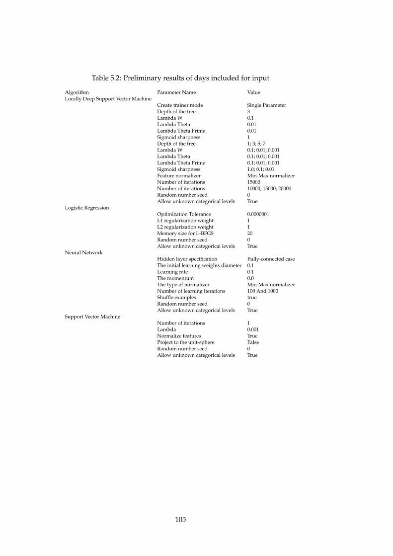
Table 5.2: Preliminary results of days included for input

Algorithm Parameter Name ValueLocally Deep Support Vector Machine

Create trainer mode Single ParameterDepth of the tree 3Lambda W 0.1Lambda Theta 0.01Lambda Theta Prime 0.01Sigmoid sharpness 1Depth of the tree 1; 3; 5; 7Lambda W 0.1; 0.01; 0.001Lambda Theta 0.1; 0.01; 0.001Lambda Theta Prime 0.1; 0.01; 0.001Sigmoid sharpness 1.0; 0.1; 0.01Feature normalizer Min-Max normalizerNumber of iterations 15000Number of iterations 10000; 15000; 20000Random number seed 0Allow unknown categorical levels True

Logistic RegressionOptimization Tolerance 0.0000001L1 regularization weight 1L2 regularization weight 1Memory size for L-BFGS 20Random number seed 0Allow unknown categorical levels True

Neural NetworkHidden layer specification Fully-connected caseThe initial learning weights diameter 0.1Learning rate 0.1The momentum 0.0The type of normalizer Min-Max normalizerNumber of learning iterations 100 And 1000Shuffle examples trueRandom number seed 0Allow unknown categorical levels True

Support Vector MachineNumber of iterations 1Lambda 0.001Normalize features TrueProject to the unit-sphere FalseRandom number seed 0Allow unknown categorical levels True

105