Embed Size (px)
Citation preview

Saarland UniversityFaculty of Natural Sciences and Technology I
Department of Computer ScienceBachelor’s Program in Computer Science
Bachelor’s Thesis
Predicting Security Vulnerabilities from Function Calls
submitted by
Christian Holler
on September 26, 2007
Supervisor: Prof. Andreas Zeller
Advisor: Dipl. Inform. Stephan Neuhaus
Reviewers: Prof. Andreas ZellerProf. Wolfgang J. Paul

Statement
Hereby I confirm that this thesis is my own work and that I have docu-mented all sources used.
Saarbruecken, September 26, 2007
Christian Holler
Declaration of Consent
Herewith I agree that my thesis will be made available through the li-brary of the Computer Science Department.
Saarbruecken, September 26, 2007
Christian Holler

Contents
1 Introduction 5
2 Related Work 7
3 Method and Implementation 93.1 General Definitions and Information . . . . . . . . . . . . . . . . . . 9
3.1.1 Definitions . . . . . . . . . . . . . . . . . . . . . . . . . . . 93.1.2 Environment . . . . . . . . . . . . . . . . . . . . . . . . . . 10
3.2 Feature Extraction from Source Code . . . . . . . . . . . . . . . . . 113.2.1 Function Calls . . . . . . . . . . . . . . . . . . . . . . . . . 113.2.2 Implementation . . . . . . . . . . . . . . . . . . . . . . . . . 13
3.3 Automated Testing . . . . . . . . . . . . . . . . . . . . . . . . . . . 133.3.1 Classification . . . . . . . . . . . . . . . . . . . . . . . . . . 143.3.2 Regression . . . . . . . . . . . . . . . . . . . . . . . . . . . 153.3.3 Implementation . . . . . . . . . . . . . . . . . . . . . . . . . 17
3.4 On-Road Test . . . . . . . . . . . . . . . . . . . . . . . . . . . . . . 183.4.1 Test Setup . . . . . . . . . . . . . . . . . . . . . . . . . . . . 183.4.2 Implementation . . . . . . . . . . . . . . . . . . . . . . . . . 18
3.5 Performance . . . . . . . . . . . . . . . . . . . . . . . . . . . . . . . 19
4 Evaluation of Results 234.1 Automated Testing Results . . . . . . . . . . . . . . . . . . . . . . . 23
4.1.1 Classification . . . . . . . . . . . . . . . . . . . . . . . . . . 234.1.2 Regression . . . . . . . . . . . . . . . . . . . . . . . . . . . 24
4.2 On-Road Test Results . . . . . . . . . . . . . . . . . . . . . . . . . . 25
5 Threats to Validity 27
6 Conclusion and Future Work 31
3

4 CONTENTS

Chapter 1
Introduction
Security vulnerabilities in software do not only pose a risk to our data and privacy butalso cause major financial loss1. Unfortunately, such vulnerabilities are hard to find,especially in huge projects, and searching for them is not only a time-consuming butalso an expensive process. Of course, one could completely avoid security vulnerabili-ties by completely specifying the software and then proving the correctness, however,this is rarely done nowadays, mainly because the complexity makes the whole processvery expensive and time consuming.In this thesis, we will see a statistical approach to aid in this search. More precisely,I will evaluate the suitability of functions calls as statistical predictors for securityvulnerabilities, using the Mozilla Project [2] source code and a provided database ofknown vulnerabilities. The main reason for the choice of function calls as a predictor isthat the Vulture project [1] has already reported good results with imports as a predictor.The required database was previously mined from the Mozilla CVS and contains allknown security vulnerabilities from 2005 to January 2007. Figure 1.1 explains therelationship between all involved elements, both the vulnerability database and thesource code serve as an input for our machine learning process which again creates apredictor that can be used for several purposes. In this case, a new component is testedto find out how likely it is to contain vulnerabilities. More information on Mozilla, themining process and vulnerabilities can be found in Section 3.1.The first question that arises when we look at vulnerabilities and function calls is mostlikely
“Are there correlations between function calls and security vulnerabilities?”
If we find such a correlation, we need to evaluate if it is suitable to predict vulnera-bilities. This step is described in Section 3.3. If the evaluation shows an acceptableaccuracy, this correlation could be used to narrow down the search space for unknownvulnerabilities in large projects, effectively saving time and money. Another questionconsequently is
“Can these correlations be used to accurately predict security vulnerabilities?”
If this is the case, this method could also be used for several other practical applica-tions. For example developers could be alerted when they introduce new code that
1An FBI study published in 2005 states a loss of 67 billion USD through computer crime
5

6 CHAPTER 1. INTRODUCTION
contains possibly risky patterns of function calls, preventing security vulnerabilitiesfrom reaching production code. So we ask ourselves
“How well does this method work in practice?”
Both to answer this question and to give an example for predicting, I will compile a listof newly found vulnerabilities in the period from January to July 2007 and evaluate,how well these vulnerabilities can be predicted using a “leave one out”-method to dopredictions for single components (See Section 3.4).
Known Vulnerabilities
Machine Learning
Newcomponent
Predictor
Codebase
produces
predicts vulnerability
CodeCode
Features
Component Vulnerability Mapping
provides
provides
Component Features Mapping
Figure 1.1: Relationship between CVS, vulnerabilities and predictions
Chapter 2
Related Work
As already mentioned in the introduction, this thesis is based directly on the Vultureproject [1], developed by Stephan Neuhaus et al., where they evaluate the quality of im-ports as a predictor in a similar way. Because their evaluation showed good results andfunction calls provide more detailed information as compared to imports, the resultsfor function calls are expected to be even better.The idea of looking at the history of components was already applied in a work bySchroter et al. [19] who investigated correlations between imports and general defects.However, this work was not focusing on security vulnerabilities.
Further related studies are:
The evolution of defect numbers, researched by both Ozment et al. [11] and Li etal. [10]. These studies deal with the evolution of the numbers of security vulner-abilities and defects over the time and came to different conclusions. Ozment etal. report a decrease in the rate at which new vulnerabilities are reported, while Liet al. report an increase. However, neither allow a mapping between componentsand vulnerabilities or a prediction.
Describing security vulnerabilities with models, researched by Chen et al. [15]. Intheir paper they deal with the difficult task to depict and reason about securityvulnerabilities using data from bugtraq and source code examination. This workand mine have in common that both a vulnerability database and the source codeare used as starting point. Chen et al. use finite state machines to model vulnera-bilities and using this model, many common types of vulnerabilities are decom-posed to simple predicates to understand how and why they occur, however, theydo not predict new vulnerabilities.
More practical approaches to reduce the number of security vulnerabilities, include:
Testing the binary. These approaches are directed at the running program and com-prehend methods like fuzz testing [16, 17] and fault injection [14]. Briefly, thesemethods find vulnerabilities by provoking faults with either specially synthesizedor random input and monitoring the program behavior.
Static source code analysis, focusing on specific types/forms of security vulnerabili-ties. Specifically, there are several tools for the detection of buffer overflows inC and C++ such as “Mjolnir”, described by M. Weber et al. in their work [12].
7

8 CHAPTER 2. RELATED WORK
There are also more generic scanners, such as ITS4, a security vulnerability scan-ner for C and C++ code developed by Viega et al. [13]. This scanner is basedon known risky patterns that are often associated with security vulnerabilities.However, most of these methods are either specific to one or several types ofvulnerabilities, or require static patterns (used in ITS4), that need to be updatedconstantly. Also, such methods might not able to recognize vulnerabilities whichhave a bigger context, across several components.
Runtime detection and prevention of exploits. There are implementations for run-time countermeasures available for the Linux kernel, such as PaX which is apart of the grsecurity package [7]. PaX generally aims at preventing any formof arbitrary code execution, e.g. through buffer overflows or heap corruption.Grsecurity also implements other methods to lower the risks of a successful at-tack, such as role-based access control lists. Another familiar implementation ofrole-based ACLs is SELinux [9].
However, these methods were not designed to find and prevent security vulnera-bilities, but to lower chance for a successful exploit and its impact once an exploitwas successful.

Chapter 3
Method and Implementation
3.1 General Definitions and Information
As stated before, the Mozilla project plays an important role because it is used for allevaluations described in this thesis. We should therefore have a look at relevant datafrom this project, especially at the process of discovering/fixing vulnerabilities and howmany vulnerabilities have been discovered in the past.Mozilla is a fairly large project, it currently consists of 10452 C/C++ components (seeDefinition 3.1) and lots of additional javascript files. The source code has a total size ofabout 800 megabytes. Since 2005, the project of course had several security problems,and in total, 424 components were affected by security vulnerabilities. Compared tothe total number of components, this is a very low percentage (approximately 4%).The process of reporting, publishing and fixing vulnerabilities has been standardizedin the Mozilla project. Vulnerabilities are reported using Bugzilla1, a bug manage-ment system developed by the Mozilla group. Reports are generally filed by the personthat discovered the vulnerability; most times these are Mozilla developers or externalpeople such as security specialists and other developers. However, sometimes vulner-abilities are discovered because they are already being exploited in the wild (0-dayexploit).Each report has a unique bugid and every CVS commit that is associated with this bugincludes the bugid for later reference. This is an important fact for definition 3.3. Oncea bug has been confirmed and fixed, the report is closed. If the bug was security related,a Mozilla Foundation Security Advisory (MFSA) is published2, as soon as fixed versionof the product is released.
3.1.1 Definitions
Some of the terms used in this thesis have no universally valid definition. In order toaid reproduction of my results, we therefore define some core terms.
Definition 3.1 (Component). Unlike in other languages such as Java, declarations anddefinitions in C/C++ often reside in different files. Declarations are made in header files
1http://www.bugzilla.org/2See http://www.mozilla.org/projects/security/known-vulnerabilities.html for a list
9

10 CHAPTER 3. METHOD AND IMPLEMENTATION
whereas definitions are made in the corresponding source file3. Nevertheless, these filesform an unseparable entity that we consider as a component.This model is suitable because a security vulnerability that affects one of these files ofcourse affects the whole component. It makes no sense to assign a vulnerability onlyto a source file, for example, and not to its corresponding header file.
Definition 3.2 (Component Naming Convention). To give components unique names,each component name starts with its path relative to the toplevel Mozilla directory. Inmany cases, there is a header and a source file as described previously. In this case, thefile extensions are omitted for component naming. Sometimes though, a componentconsists of a single file, in this case, the component name will contain the full filenameincluding the file extension. The following examples clarify this:
mozilla # ls xpinstall/src/nsInstallResources*xpinstall/src/nsInstallResources.cppxpinstall/src/nsInstallResources.h
−→ Component name: xpinstall/src/nsInstallResources
mozilla # ls js/src/jsbit*js/src/jsbit.h
−→ Component name: js/src/jsbit.h
Of course, to reference to a specific component in this document the path may beomitted where this does not cause any ambiguities.
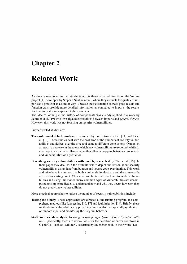
Definition 3.3 (Vulnerable Component). To associate components with vulnerabil-ities, we will obtain the bugids for vulnerabilities from the Mozilla security advisorywebsite and then use the Mozilla CVS to search for changes that contain this bugid, asshown in Figure 3.1. As explained earlier in this chapter, all changes that are related toa given bugreport include the bug id in the commit message.Therefore we consider every component as vulnerable that has a change log containinga bugid that is associated with a vulnerability. However, this definition is very broadand has some problems, see Section 5 for possible problems with this definition.
Definition 3.4 (Neutral Component). A component is neutral when it is not vulner-able according to definition 3.3. The word “neutral” especially implies that we donot know exactly whether this component actually has an undiscovered vulnerability.Therefore, “neutral” should never be mixed up with “invulnerable” as there might bevulnerabilities present that nobody is aware of.
3.1.2 EnvironmentAll programs that were written in the course of this thesis were in Perl [3] and R [4].Perl is used for parsing, preprocessing of input data and postprocessing of results,whereas R is used for the actual predictions. Especially for our machine learning parts,the e1071 [6] package for R provides the required algorithms. Also, e1071 is one ofthe few packages that support sparse matrices for several algorithms during the wholeprocess of computing and predicting. As we will see later, this provides a great speedup
3This is an idealized model, in practice, short definitions are often placed in header files directly anddeclarations can also be made in source files.
3.2. FEATURE EXTRACTION FROM SOURCE CODE 11
Security Advisory Changes Components
Figure 3.1: Mapping vulnerabilities to components through advisories and bug reports
for predictions. Although all programs were written for Linux, they could also rununder Windows with slight modifications since both Perl and R exist for Windows aswell.
3.2 Feature Extraction from Source Code
3.2.1 Function Calls
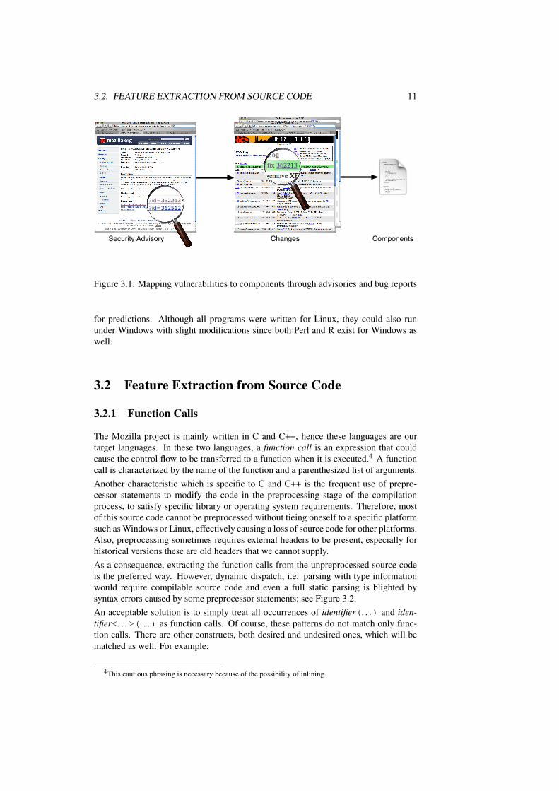
The Mozilla project is mainly written in C and C++, hence these languages are ourtarget languages. In these two languages, a function call is an expression that couldcause the control flow to be transferred to a function when it is executed.4 A functioncall is characterized by the name of the function and a parenthesized list of arguments.Another characteristic which is specific to C and C++ is the frequent use of prepro-cessor statements to modify the code in the preprocessing stage of the compilationprocess, to satisfy specific library or operating system requirements. Therefore, mostof this source code cannot be preprocessed without tieing oneself to a specific platformsuch as Windows or Linux, effectively causing a loss of source code for other platforms.Also, preprocessing sometimes requires external headers to be present, especially forhistorical versions these are old headers that we cannot supply.As a consequence, extracting the function calls from the unpreprocessed source codeis the preferred way. However, dynamic dispatch, i.e. parsing with type informationwould require compilable source code and even a full static parsing is blighted bysyntax errors caused by some preprocessor statements; see Figure 3.2.An acceptable solution is to simply treat all occurrences of identifier(. . .) and iden-tifier<. . .>(. . .) as function calls. Of course, these patterns do not match only func-tion calls. There are other constructs, both desired and undesired ones, which will bematched as well. For example:
4This cautious phrasing is necessary because of the possibility of inlining.
12 CHAPTER 3. METHOD AND IMPLEMENTATION
Function definitions
JS_PUBLIC_API(int64) JS_Now() { return PRMJ_Now(); }
Extern Forward declarations
extern JS_PUBLIC_API(int64) JS_Now();
Macro calls
MOZ_COUNT_CTOR(nsInstallLogComment);
Constructor calls
ie = new nsInstallFile( this, [...] );
Some keywords
if (buffer == nsnull || !mInstall) return 0;
Initialization lists
nsXPItem::nsXPItem(const PRUnichar* aName) : mName(aName)
C++ functional-style casts
int(curWidget->fieldlen.length)
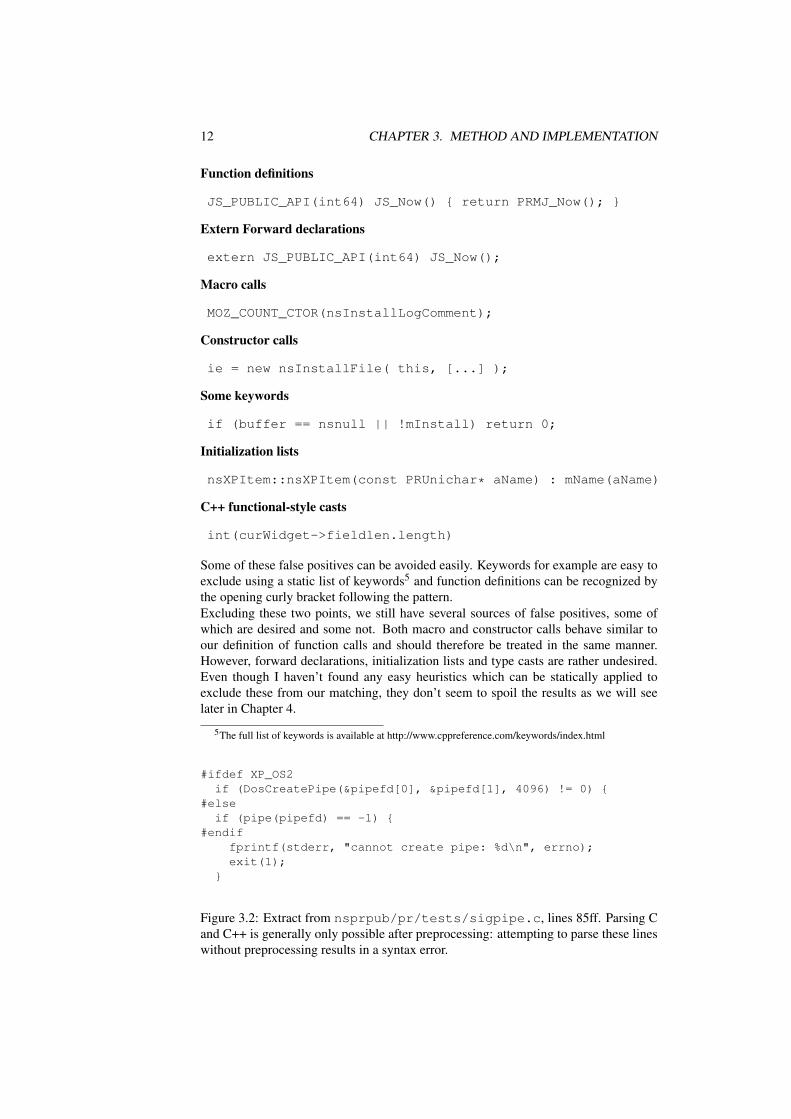
Some of these false positives can be avoided easily. Keywords for example are easy toexclude using a static list of keywords5 and function definitions can be recognized bythe opening curly bracket following the pattern.Excluding these two points, we still have several sources of false positives, some ofwhich are desired and some not. Both macro and constructor calls behave similar toour definition of function calls and should therefore be treated in the same manner.However, forward declarations, initialization lists and type casts are rather undesired.Even though I haven’t found any easy heuristics which can be statically applied toexclude these from our matching, they don’t seem to spoil the results as we will seelater in Chapter 4.
5The full list of keywords is available at http://www.cppreference.com/keywords/index.html
#ifdef XP_OS2if (DosCreatePipe(&pipefd[0], &pipefd[1], 4096) != 0) {
#elseif (pipe(pipefd) == -1) {
#endiffprintf(stderr, "cannot create pipe: %d\n", errno);exit(1);
}
Figure 3.2: Extract from nsprpub/pr/tests/sigpipe.c, lines 85ff. Parsing Cand C++ is generally only possible after preprocessing: attempting to parse these lineswithout preprocessing results in a syntax error.

3.3. AUTOMATED TESTING 13
3.2.2 ImplementationThe final parser includes all methods to identify function calls as described above aswell as common parsing methods such as exclusion of comments, strings and prepro-cessor statements from our search space. It takes up only 9 kilobytes or 346 lines ofcode.The parser takes all files, that belong to the component to analyze, as parameters. Af-ter extracting the function calls from those files, it determines the component nameaccording to Section 3.2 and outputs the results in the following format:
<component name>: functionA/count functionB/count [...]
Example:
js/src/jsstr: AddCharsToURI/6 js_ExecuteRegExp/4 [...]
Because the parser outputs its results for a single component, a second tool is requiredthat invokes the parser with the respective files. This tool is called the project parserand goes through the project directory structure, searching for relevant files, groupingthem together into components and then invokes the parser for each file group.For more information about the parser speed on the whole project, see Section 3.5.
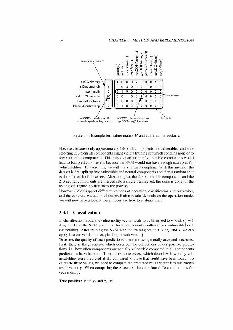
3.3 Automated TestingThe data provided by the parser can be interpreted as a matrix M which represents therelationships between all functions f j in the project and its components ci . The matrixentries describe the number of occurrences of a function within a component, i.e. mi jis the number of occurrences of the function f j in the component ci .Using the provided data about past vulnerabilities in the project, we can also associateeach component ci with a value vi indicating the number of past vulnerabilities in thiscomponent, yielding a vector v called the vulnerability vector.Figure 3.3 shows an example for M and v with fictitious values. Both M and v togetherform the basis for all further experiments and their evaluation.To find statistical correlations between function calls and vulnerabilities in this dataset,we will use machine learning. When using machine learning, generally a model f iscreated using a suitable training set. The general recommendation for the size of thistraining set is 2/3 of the whole dataset and we will follow this recommendation for ourevaluation setup. The general idea is to split up the dataset into two parts,
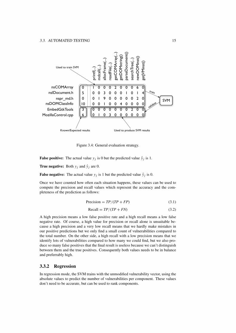
the training set which consists of the matrix MT and the vector x, the parts of v thatcorrespond to MT , and
the validation set which consists of the matrix MV and the vector y, the parts of v thatcorrespond to MV ,
and then use the training set to generate a model f that we can apply to the validationset.In our case, we will use Support Vector Machines [5] as a special case for machinelearning, because SVMs can also handle data that is not linearly separable. Also, theyare less prone to overfitting than other machine-learning methods, such as k-nearest-neighbors[20].
14 CHAPTER 3. METHOD AND IMPLEMENTATION
10 4
1 0 0 0 2 0 0 0 6 00 0 3 0 0 0 1 0 1 40 1 9 0 0 0 0 0 2 00 0 1 0 0 0 0 0 00 0 0 0 0 0 0 2 0 00 1 0 3 0 0 0 0 0 0
prin
tf(..
.)m
dcal
l(...)
new
DO
Min
st()
read
File
(...)
allo
cFra
me(
...)
getJ
VM
inst
()
sear
chTr
ee(..
.)
pars
eDoc
umen
t()
getD
OM
stri
ng()
getC
OM
Arr
ay(..
.)
nsIDocument.h050
00
nsCOMArray
nsDOMClassInfonspr_md.h
EmbedGtkToolsMozillaControl.cpp
nsDOMClassInfo has had 10vulnerability-related bug reports
nsDOMClassInfo calls function"getDOMstring()" four times
Matrix M
Vulnerability vector v
Row vector
Figure 3.3: Example for feature matrix M and vulnerability vector v.
However, because only approximately 4% of all components are vulnerable, randomlyselecting 2/3 from all components might yield a training set which contains none or tofew vulnerable components. This biased distribution of vulnerable components wouldlead to bad prediction results because the SVM would not have enough examples forvulnerabilities. To avoid this, we will use stratified sampling. With this method, thedataset is first split up into vulnerable and neutral components and then a random splitis done for each of these sets. After doing so, the 2/3 vulnerable components and the2/3 neutral components are merged into a single training set, the same is done for thetesting set. Figure 3.5 illustrates the process.However SVMs support different methods of operation, classification and regression,and the concrete evaluation of the prediction results depends on the operation mode.We will now have a look at these modes and how to evaluate them.
3.3.1 Classification
In classification mode, the vulnerability vector needs to be binarized to v′ with v′
j = 1if v j > 0 and the SVM prediction for a component is either 0 (not vulnerable) or 1(vulnerable). After training the SVM with the training set, that is MT and x, we canapply it to our validation set, yielding a result vector y.To assess the quality of such predictions, there are two generally accepted measures.First, there is the precision, which describes the correctness of our positive predic-tions, i.e. how often components are actually vulnerable compared to all componentspredicted to be vulnerable. Then, there is the recall, which describes how many vul-nerabilities were predicted at all, compared to those that could have been found. Tocalculate these values, we need to compare the predicted result vector y to our knownresult vector y. When comparing these vectors, there are four different situations foreach index j :
True positive: Both y j and y j are 1.
3.3. AUTOMATED TESTING 15
10 4
1 0 0 0 2 0 0 0 6 00 0 3 0 0 0 1 0 1 40 1 9 0 0 0 0 0 2 00 0 1 0 0 0 0 0 00 0 0 0 0 0 0 2 0 00 1 0 3 0 0 0 0 0 0
prin
tf(..
.)m
dcal
l(...)
new
DO
Min
st()
read
File
(...)
allo
cFra
me(
...)
getJ
VM
inst
()
sear
chTr
ee(..
.)
pars
eDoc
umen
t()
getD
OM
stri
ng()
getC
OM
Arr
ay(..
.)
nsIDocument.h050
36
nsCOMArray
nsDOMClassInfonspr_md.h
EmbedGtkToolsMozillaControl.cpp
Used to train SVM
Used to produce SVM results
validate
train
Known/Expected results
SVM
Figure 3.4: General evaluation strategy.
False positive: The actual value y j is 0 but the predicted value y j is 1.
True negative: Both y j and y j are 0.
False negative: The actual value y j is 1 but the predicted value y j is 0.
Once we have counted how often each situation happens, these values can be used tocompute the precision and recall values which represent the accuracy and the com-pleteness of the prediction as follows:
Precision = TP/(TP + FP) (3.1)
Recall = TP/(TP + FN) (3.2)
A high precision means a low false positive rate and a high recall means a low falsenegative rate. Of course, a high value for precision or recall alone is unsuitable be-cause a high precision and a very low recall means that we hardly make mistakes inour positive predictions but we only find a small count of vulnerabilities compared tothe total number. On the other side, a high recall with a low precision means that weidentify lots of vulnerabilities compared to how many we could find, but we also pro-duce so many false positives that the final result is useless because we can’t distinguishbetween them and the true positives. Consequently both values needs to be in balanceand preferrably high.
3.3.2 RegressionIn regression mode, the SVM trains with the unmodified vulnerability vector, using theabsolute values to predict the number of vulnerabilities per component. These valuesdon’t need to be accurate, but can be used to rank components.

16 CHAPTER 3. METHOD AND IMPLEMENTATION
Components
Neutral components
Vulnerable components
2/3neutral
1/3 neutral
2/3 vulnerable
1/3 vulnerable
Rand
om s
plit Training set
Validation set
Figure 3.5: Stratified sampling.
True Positive (TP)
False Negative (FN)
Actually hasvulnerability reports
yes no
yes
no
Predicted to havevulnerability reports
Precision
Recall
True Negative (TN)
False Positive (FP)
Figure 3.6: Precision (TP/(TP + FP)) and recall (TP/(TP + FN)).
Being able to produce a ranking of the most vulnerable components, especially forthose that do only have few or even no known vulnerabilities, could help developersfocus their efforts on a smaller group of components, effectively maximizing their suc-cess in finding vulnerabilities whilst minimizing effort.The reviewers of the Vulture paper [1] rejected the use of the Spearman Rank Corre-lation Coefficient [18] to evaluate how exact the predicted ranking reflects the actualranking. Instead, they suggested a cost model that matches the practical scenario wherea manager has to distribute limited resources to audit components:Assuming that we have the resources to test T components, then these would be bestspent on the top T most vulnerable components, however the order inbetween thesetop T is irrelevant. Ideally, the predicted top T components would be the same asthe actual top T components, no matter their order. To evaluate the quality of ourprediction, we hence could compare how many vulnerabilities we can fix with ourprediction compared to the ideal case:With m being the number of components and y being the predicted vulnerability vector,we define p = (p1, ..., pm) as a permutation of 1, ..., m such that yp = (yp1 , ..., ypm ) issorted in descending order. Fixing component p j fixes yp j vulnerabilities, hence fixingthe top T predicted components fixes F =
∑1≤ j≤T yp j vulnerabilities. However, with
the optimal ordering, with q and yq defined accordingly to p and yp, we could have

3.3. AUTOMATED TESTING 17
fixed Fopt =∑
1≤ j≤T yq j vulnerabilities. We can now use the quotient Q = F/Fopt toindicate the quality of our prediction. Because 0 ≤ F ≤ Fopt, Q is a value between 0and 1 and higher values indicate a better ranking.In a typical situation, the total number of vulnerable components is much smaller thanthe number of neutral components, therefore a random selection will almost alwaysgive Q = 0 for small T . In order to be useful in practice, we hence expect a value forQ that is considerably greater than zero. A good threshold would be 0.5 which meansthat at least half of the effort was spent meaningfully.
3.3.3 Implementation
The implementation for the automated testing environment consists of several parts:
The preprocessor translates the parser output described in Section 3.2.2 into a sparsematrix format that is readable by the read.matrix.csr function providedby the e1071 package. This format is highly suitable because the matrix is onlysparsely populated and writing out the whole matrix would consume several gi-gabytes of space whereas the sparse matrix only takes up 2 megabytes. Duringthe translation, the matrix is also sorted in both dimensions using the lexical or-der of the function names and components as the sorting criteria. Additionally,filters can be applied like binarization for the data values, i.e. cutting all non-zerovalues to 1 and several filter criterias which remove functions from the matrix.One motivation for the binarization filter is that absolute values also depend onthe size of a component, so a correlation between the size and the number of vul-nerabilities could degrade the results. Of course, the preprocessor is also able tooutput the vulnerability vector, a index-to-component mapping and several otheruseful pieces of information.
The R scripts are responsible for splitting our data as well as training the SVM and us-ing it to predict the vulnerabilities for our validation set. After reading the sparsematrix and the vulnerability vector, a stratified sampling is done and the trainingprocess is started with the training set. Once the SVM is trained, the predictionis done for the testing set and results are written to the terminal. For classifica-tion, this is simply the table containing the true/false positives/negatives, but forregression, the scripts already outputs the results as described in Section 3.3.2.Additionally, each script outputs its random split indices into a file to allow re-production of our results.
The simulator supervises the execution of the R scripts. To rule out that the resultsare only good for one random split, the simulator supports repeating the samescript for a given amount of time, each time using a different random split andall results are collectively written to one file. Even though a single predictionprocess is quite fast, the simulator supports threading for an additional speedgain on multiprocessor systems.
Several evaluation scripts are then used to summarize a result file for a simulationinstance, e.g. calculating the median of result values; see Figure 3.7

18 CHAPTER 3. METHOD AND IMPLEMENTATION
3.4 On-Road TestIn addition to the automated tests described above, an on-road test with the Mozillaproject and current vulnerabilities would demonstrate that this is indeed a method forpractical use. Therefore I decided to do such a test and the setup is described below.
3.4.1 Test SetupThe automated tests used in this thesis only have information about vulnerabilitiesdiscovered up to January, 2007; however, at the time of test, it was already July andlots of new vulnerabilities were discovered. A sensible step would be to use these newvulnerabilities to test the predictive power of our method. In the first step, we henceneed to find all vulnerabilities and map these to components according to Section 3.3.The second step is prediction and evaluation. The prediction will work using a “leaveone out”-method, in detail a single prediction will be done as follows:Assuming that we want a prediction for component j (1 ≤ j ≤ m), we use all com-ponents (1, . . . , m), except the component j itself, to train the SVM. After doing so,the SVM is used to predict the component j . These steps will be done in regressionmode because regression allows us to better extract a small number of components thatare very likely to be vulnerable. Figure 3.8 illustrates a prediction step for a singlecomponent.In our test, the above steps will be done for all components 1, ..., m and the result foreach component is recorded. Of course we will use the old vulnerability vector thatdoes not contain the new vulnerabilities to do our predictions. After the whole testis finished, we will look at the predicted top 20 of components that were previouslyflagged as neutral and see how many of them are now affected by a new vulnerabilityand how the vulnerability affects the component6.
3.4.2 ImplementationPrior to any implementation, we first have to get information about new vulnera-bilities. We can extract these from http://www.mozilla.org/projects/security/known-vulnerabilities.html. All Mozilla security advisories are listed there with there respec-tive bugzilla bugid. For our purpose, I compiled a list of new vulnerabilities by hand ina simple parseable format, listing the MFSA and all bugids related to this MFSA.Of course, this information could also be parsed from the Mozilla website automati-cally7, but in this case, it was easier to compile the list by hand. In addition to this list,we need the full Mozilla CVS which takes about 3.6 gigabytes of downloading. Withthese requirements satisfied, the automated scripts can do the rest. They again consistof several parts:
The CVS parser gets the vulnerability list as input and searches through the CVSlog of each file looking for bugids that are mentioned in this list. It outputs allcomponents that are affected by any of these bugids with the MFSA number andthe bugid. If a component is affected by two MFSAs and/or bugids, the parseroutputs the component twice with the respective information. This is essentiallya simple re-implementation of the algorithm outlined in the Vulture paper.
6Inspecting how a vulnerability affects a component of course does not work automatically but requiresa qualified human.
7The Vulture project includes a parser for this task.
3.5. PERFORMANCE 19
The parser postprocessor compares the components found by the CVS Parser to ourlist of components that are already vulnerable. For our test, we only need thecomponents that are still listed as neutral in our vulnerability vector. Addition-ally, this tool outputs more useful information, e.g how many components are“repeaters”8.
An R script reads the vulnerability matrix and vector and then starts the “leave oneout” prediction, outputting the results for each component into a single file.
An evaluation script reads these results, calculates the top 20 of components thatwere previously listed a neutral and are now predicted to be vulnerable, withthe predicted number of vulnerabilities as sorting criteria. Then it compares,how many of these components are actually vulnerable now according to ournew vulnerability data.
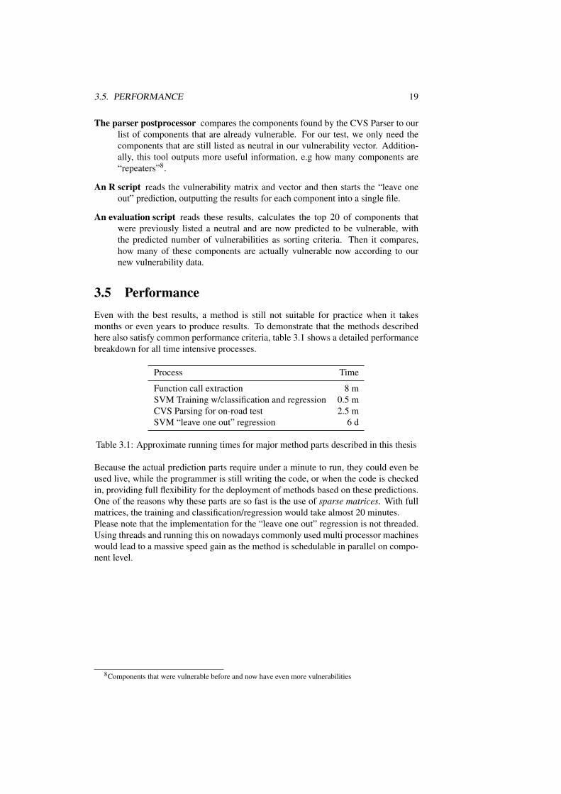
3.5 PerformanceEven with the best results, a method is still not suitable for practice when it takesmonths or even years to produce results. To demonstrate that the methods describedhere also satisfy common performance criteria, table 3.1 shows a detailed performancebreakdown for all time intensive processes.
Process Time
Function call extraction 8 mSVM Training w/classification and regression 0.5 mCVS Parsing for on-road test 2.5 mSVM “leave one out” regression 6 d
Table 3.1: Approximate running times for major method parts described in this thesis
Because the actual prediction parts require under a minute to run, they could even beused live, while the programmer is still writing the code, or when the code is checkedin, providing full flexibility for the deployment of methods based on these predictions.One of the reasons why these parts are so fast is the use of sparse matrices. With fullmatrices, the training and classification/regression would take almost 20 minutes.Please note that the implementation for the “leave one out” regression is not threaded.Using threads and running this on nowadays commonly used multi processor machineswould lead to a massive speed gain as the method is schedulable in parallel on compo-nent level.
8Components that were vulnerable before and now have even more vulnerabilities

20 CHAPTER 3. METHOD AND IMPLEMENTATION
Preprocessor
Simulator
produces
runs
CodeCodeParser output
Vulnerability Mapping
Sparse Matrix&
Vulnerability Vector
R Scripts
CodeCode
Results
producescollects
Result file
produces
Parser
Evaluation Scripts
Summary
Figure 3.7: Interaction between implementation parts

3.5. PERFORMANCE 21
SVMCode
CodeComponents
Component to test
CodeOther
components
train
predict
split
Figure 3.8: Single step in “leave one out” prediction
# MFSA bugid [bugid ..]2007-25 369211 3701272007-24 3873332007-23 384384
Figure 3.9: New vulnerabilities since January 2007 in simple format, hand compiled.

22 CHAPTER 3. METHOD AND IMPLEMENTATION
Chapter 4
Evaluation of Results
4.1 Automated Testing ResultsIn this section we will have a look at the results for our automated tests described inSection 3.3. However, we will not only look at the best results, but also at other settingsfor our matrix preprocessor and see how they changed the results. These are:
• The “binary” setting, each matrix entry mi j is replaced with 1 if mi j > 0 andelse with 0.
• The “stripped” setting, functions which only appear in one component are ig-nored, as well as function names with a length of 2 or less. The aim is to removeirrelevant functions to improve the results. When using this setting, the matrixwidth is reduced from 93265 to 40224, however, the execution time is hardlyaffected.
Both for classification and regression however, it turned out that using the “binary” set-ting leads to better results, even though binary values provide less precise information.
4.1.1 ClassificationFor classification, we measure precision and recall for our evaluation as described inSection 3.3.1. Table 4.1 shows the median results for several settings, based on 100splits for each setting.
Dataset Precision Recall
Original 50.77% 40.41%Binary 69.95% 40.14%Stripped 49.08% 40.94%Binary and stripped 64.61% 43.71%
Table 4.1: Median values according to cost model described in Section 3.3.2 acrossdifferent datasets
The results do not only show that binary values lead to a much better result, but alsothat the SVM is able to handle unimportant data that is removed by our filters, the
23

24 CHAPTER 4. EVALUATION OF RESULTS
results are almost the same. Figure 4.1 shows the detailed distribution of all 100 pairsfor the binary dataset. But even more important, for the best dataset
70% of all predictions are correct,and 40% of all known vulnerabilities were found.
When we compare this to a random selection, with 10452 components and only 424vulnerable (approx. 4%), then we see that these values provide a tremendous advantageto simple random guessing.
●
●
●
●
●
●●
●
●●
●
●●
●
●
●●
●
●●
●
●●
●
●
●●●
●●
●●
●
●●
●●
●
●
●
●●
●
●●
●
●●
●
●
●●
●
●
●
●
●●
●
●
●●
●
●●
●●
●●
●
●●
●
●
●
●●
●
●●●●
●
●●●●
●
●
● ●
●
●
●
●
●●
●
●●
0.30 0.35 0.40 0.45 0.50
0.55
0.60
0.65
0.70
0.75
0.80
Recall
Pre
cisi
on
Figure 4.1: Scatterplot for 100 precision/recall pairs
4.1.2 Regression
Dataset Top 10 Top 30
Original 73.33% 72.19%Binary 80.91% 84.81%Stripped 75% 68.28%Binary and stripped 82.47% 83.33%
Table 4.2: Median values for top 10 and top 30 across different datasets
As expected, the distribution of results across the different datasets is similar to theresults in classification and the binary datasets gives the best results. However, in thiscase we see that the stripped binary dataset is slightly better than the binary set, howeverthese are only minor differences. With the stripped binary set

4.2. ON-ROAD TEST RESULTS 25
82% of all possible top 10 vulnerabilities and 83% of all possible top 30vulnerabilities were found.
As already explained in Section 3.3.2, with the ratio of vulnerable components to neu-tral components being very low (roughly 1:25), a random selection would almost al-ways lead to a total of 0 vulnerabilities found.
4.2 On-Road Test Results
Since January 2007, 68 components that were neutral needed to be fixed because ofvulnerabilities by July 2007. After examining the predicted top 20 of all 10028 neutralcomponents, a total of 6 components were now actually affected by one or more newvulnerabilities. That means with only 0.678% of components that are now vulnerable,we found 8.8% only by looking at the Top 20, i.e. more than twelve times the amountof vulnerabilities compared to a random selection. After inspecting the bug reports andCVS commit messages of these vulnerabilities, it was clear that all except one of thesecomponents were either the source of the vulnerability or directly involved with thevulnerable component. The remaining component that was predicted to be at rank 1,turned out to be a false positive. A version string inside the component was changedwith a vulnerability bugid in the commit message, however, the component had nodirect relation to the vulnerability. Figure 4.3 shows the list of relevant componentsand their result of manual inspection.
# Component Name Bug Id Detailed information
2 jsscope Bug 381374 Assertion failure in component,allowing to crash program
Bug 364657 Possible crash in another component,fix includes major code addition tothis component
7 nsSliderFrame Bug 344228 Component was using thensIScrollbarMediatorcomponent in an insecure way
9 nsTableRowFrame Bug 370360 Actual bug innsTableRowGroupFrame butcomponents seem very similar intheir domain
10 nsFrameManager Bug 343293 Crash bug, missing assertions andchecks in this component
nsFrameManager Bug 363813 Component not directly affected butsource code changes made becauseof this bug
18 nsIContent.h Bug 382754 Bug report not publically accessiblebut CVS shows that this is one oftwo files changed with identicalcommit message
Table 4.3: Components in our prediction that are now actually vulnerable, with # indi-cating the predicted rank

26 CHAPTER 4. EVALUATION OF RESULTS
With 4 hits in the predicted top 10, based on the vulnerabilities discovered in only halfa year, this is a really good result. If the Mozilla team had received this information inJanuary, they could have found these vulnerabilities even faster by concentrating theirefforts on the top 10 of our prediction. Altogether, the on-road test showed that thismethod is indeed providing excellent results, suitable for practical application.

Chapter 5
Threats to Validity
There are several possible threats to the validity of my work, those are:
Limited target codebase used for evaluation. The whole process of predicting andevaluating was done with a single project, the Mozilla Project. Hence, the ob-served correlations could be specific to this project only. However, it seems un-likely that the Mozilla Project is such a special project compared to other majorcodebases, so this is rather a minor threat.
Defective tools. The tools used in this thesis might contain bugs themselves that leadto falsified results. This is not unlikely, I personally found 2 bugs in the sparsematrix implementation of e1071. However, the Vulture project was using fullmatrices in an earlier stage and we verified the Vulture results using the sparseimplementation and the chance that both the sparse and the full implementationsuffer from the same bug is very low.
Inaccurate feature extraction. In Section 3.2 we already saw that it is not perfectlypossible to statically extract function calls from C/C++ source code. The inac-curacy in this process could lead to falsified input data, however the results don’tseem to be spoiled by this.
Broad definition of “vulnerable”. In general, we call a component vulnerable whenit is directly affected by a security vulnerability, however when doing automatedmining of these information, it is often not decidable whether a component is ac-tually affected by a vulnerability in the context of security. When a vulnerabilityis fixed, other components require changes sometimes, because a component orfunction interface changed, without however being directly affected by the se-curity impact of the vulnerability. This would lead both to inaccurate input (inthe vulnerability mapping) and inaccurate comparative data (e.g. in the on-roadtest). A good example here is a component that was on rank 1 of our predictionin the on-road test, but the change that marked this component as vulnerable wasonly a version number change. The impact of this threat has yet to be evaluatedbut is not in the scope of this thesis.
Evaluation misses chronological context. A prediction always implies a chronolog-ical order, the prediction generally depends on past data and the componentsthat are analyzed lie in the present. The automated evaluation however, doesnot honor this context when doing the splits for training and validation set. This
27

28 CHAPTER 5. THREATS TO VALIDITY
could lead to better results than one would get when forcing a chronological or-der of components. The impact of this threat has yet to be evaluated but is not inthe scope of this thesis.
Evaluation misses grouping of vulnerable components. As described earlier in thissection, a vulnerability often causes multiple files to be fixed at once, be it be-cause of interface changes or because a bug spans across several components.All changed components are marked as vulnerable according to our definition inSection 3.3. See Figure 5.1 for a simple example.
However, during the automated evaluation, these groupings are broken up andeach vulnerable component is treated as if it was affected by an its own bug.Hence it is likely to happen that components that are affected by the same vul-nerability are separated, some go into the training set and some into the validationset.
If the correlations between components that suffer of a single vulnerability arestronger, than those between components that suffer from different vulnerabili-ties, then this might falsify the results. Figure 5.2 shows such a situation, wherebasically a vulnerability “predicts itself”.
The typical scenario for a prediction of new vulnerabilities though is a “past topresent” relationship between the known and the yet unknown vulnerabilities.The situation described in Figure 5.2 and hence the whole automated evaluationprocess, is therefore very unlikely in this application case and therefore, the re-sults in a practical prediction scenario could be worse than those observed in theevaluation. Figure 5.3 shows this in a simplified way.
However, it is not given that the correlations inside such a group are strongerthan the correlations between different vulnerabilities, and even if this shouldbe case, it is not possible to say to what extend the results are affected by this.Researching these effects is not in the scope of this work.
Component A
Component C
Component B
Component D
Component E
Component F
Bug 123 affects Components A, B and C
Bug 456 affects Components D, E and F
Bug 456Bug 123
Figure 5.1: Initial situation, two vulnerabilities, each affects several components.

29
Component A
Component C
Component B Component D Component E
Component F
Bug 456Bug 123Training Set
Validation Set
Random Split
Component A
Component C
Component B Component D Component E
Component F
Bug 456Bug 123 A and B leadto positive
prediction for C
D and E leadto positive
prediction for F
Figure 5.2: The random split goes across component groups.
Component A
Component C
Component B Component D Component E
Component F
Bug 456Bug 123
Known vulnerability Unknown vulnerability
Past Present
Correlation betweendifferent bugs
could be weaker
Figure 5.3: Correlation between different vulnerabilities could be weaker, making themethod less effective in a typical prediction scenario.

30 CHAPTER 5. THREATS TO VALIDITY

Chapter 6
Conclusion and Future Work
The automated evaluation tests clearly showed that there is a correlation between func-tion calls and security vulnerabilities that can be used to predict unknown vulnerabili-ties. We also saw that these predictions are not only superior to random selection underthe aspects of a cost-benefit analysis, but also highly precise (70% precision) in classifi-cation. According to our cost model for regression, our predictions also provide resultsthat can be used to greatly increase the efficiency of finding security vulnerabilities.Also, with the on-road test we saw a method for practical application in large projects,showing us that this is not a purely theoretic result.With this success, we can resolve on several future objectives:
Evaluating the method with different projects. Gathering further results with otherprojects eleminates the threat of limitation to a single project, strengthening theposition of the described methods amongst other scientific approaches.
Evaluating other features. The framework described and used in this thesis is notlimited to function calls as features. Other features could lead to even betterresults, so this is also an interesting direction of research.
IDE implementation. Implementing methods for single component prediction intoan IDE, warning developers when they code or commit something potentiallymalicious, would help to prevent vulnerabilities before they even reach the finalproject code.
However, there are several threats that have a yet unknown impact. Researching themwould help us to better understand how they affect the presented results, as well asproviding us methods to increase the accuracy of this and other methods. Basically, therequired tasks would be:
Chronological evaluation. This would require an evaluation model that respects thechronological order of vulnerabilities. From the results of such a model, wecould verify that correlations also apply in this context and possibly how predic-tors change over the time.
Assessment of file groups affected by single vulnerabilities. It is still unclear howstrong vulnerable component groups are connected to each other. If they canbe separated, then the correlation between different vulnerabilities can be exam-ined in a better way and the strength of the correlation between these and the
31

32 CHAPTER 6. CONCLUSION AND FUTURE WORK
correlation inside such a component group could be compared. Moreover, if thecorrelation in a component group affected by a single vulnerability is stronger,this could be used to point developers to related components during the processof fixing.

Bibliography
[1] S. Neuhaus, T. Zimmermann, C. Holler, A. Zeller. Predicting Vulnerable Soft-ware Components. 14th ACM Conference on Computer and CommunicationsSecurity, October 2007
[2] The Mozilla Foundation. Mozilla project website. http://www.mozilla.org/, Jan-uary 2007.
[3] Larry Wall. The Perl programming language. Perl directory.http://www.perl.org/, 1987.
[4] The R Foundation. The R Project for Statistical Computing. http://www.r-project.org/, 2003.
[5] Vladimir Naumovich Vapnik. The Nature of Statistical Learning Theory.Springer Verlag, Berlin, 1995.
[6] E. Dimitriadou, K. Hornik, F. Leisch, D. Meyer, and A. Weingessel.Misc Functions of the Department of Statistics. TU Wien. http://cran.r-project.org/src/contrib/Descriptions/e1071.html, 2006.
[7] Brad Spengler. The grsecurity project. http://grsecurity.net/.
[8] The PaX Team. PaX patches. http://pax.grsecurity.net/.
[9] National Security Agency, Network Associates Laboratories, The MITRECorporation and the Secure Computing Corporation. The SELinux Projecthttp://www.nsa.gov/selinux/, 2001.
[10] Zhenmin Li, Lin Tan, Xuanhui Wang, Shan Lu, Yuanyuan Zhou, and Chengxi-ang Zhai. Have things changed now? An empirical study of bug characteristicsin modern open source software. In Proceedings of the Workshop on Architec-tural and System Support for Improving Software Dependability 2006, pages25?33. ACM Press, October 2006.
[11] Andy Ozment and Stuart E. Schechter. Milk or wine: Does software securityimprove with age? In Proceedings of the 15th Usenix Security Symposium,pages 93-104, August 2006.
[12] M. Weber, V. Shah, and C. Ren. Cigital, Inc. A case study in detecting softwaresecurity vulnerabilities usingconstraint optimization. In Source Code Analysisand Manipulation, 2001. Proceedings., 2001
33

34 BIBLIOGRAPHY
[13] J. Viega, J.T. Bloch, Y. Kohno, G. McGraw. ITS4: A static vulnerability scannerfor C and C++ code. In 16th Annual Computer Security Applications Confer-ence (ACSAC’00) acsac, page 257, 2000
[14] Jeffrey Voas and Gary McGraw. Software Fault Injection: Innoculating Pro-grams Against Errors. John Wiley & Sons, 1997.
[15] Shuo Chen, Z. Kalbarczyk, J. Xu, R.K. Iyer. A data-driven finite state machinemodel for analyzing security vulnerabilities. Proceedings of the Conference onthe Dependable Systems and Networks, 2003.
[16] B.P. Miller, L. Fredriksen, B. So. An Empirical Study of the Reliability of UNIXUtilities. Communications of the ACM 33, 12, 1990.
[17] B.P. Miller. Fuzz Testing of Application Reliability.http://pages.cs.wisc.edu/ bart/fuzz/fuzz.html, 1990-2006.
[18] R. V. Hogg and A. T. Craig. Introduction to Mathematical Statistics, 5th ed.New York: Macmillan, pp. 338 and 400, 1995.
[19] Adrian Schroter, Thomas Zimmermann, and Andreas Zeller. Predicting com-ponent failures at design time. In Proceedings of the 5th International Sympo-sium on Empirical Software Engineering, pages 18?27, New York, NY, USA,September 2006. Association for Computing Machinery, ACM Press.
[20] Trevor Hastie, Robert Tibshirani, and Jerome Friedman. The Elements of Sta-tistical Learning: Data Mining, Inference,and Prediction, Chapter 13. SpringerSeries in Statistics. Springer Verlag, 2001.