1

Predicting radiated emissions from cables in the RE02/RE102/DO-160/SAE J113-41 test set up, using measured current in NEC and simple

TX equations.

D. A. Weston RE02Tx.rep 14-6-2004NARTE Certified EMC Engineer

THIS REPORT IS PART OF A RESEARCH PROGRAM AND THE CONTENT,OR ANY PART THEREOF, MAY BE REPRODUCED AS LONG AS THESOURCE IS RECOGNIZED AS FOLLOWS:

Reproduced by permission of EMC Consulting Inc. from the report “Predictingradiated emissions from cables in the RE02/RE102/DO-160/SAE J113-42 test set up,using measured current in the NEC and simple TX equations”.

2

1) Introduction

It is often required to predict the radiated emissions from cables in the typical radiatedemission test set up in an anechoic chamber or absorber loaded room. A set up specifiedby the military, space, civilian aircraft and automotive industries has the cable of 2m lengthat a height of 0.05m and 0.1m from the front edge of a ground plane with the measuringantenna at a distance of 1m from the Equipment Under Test (EUT)/cable. These types ofmeasurements are notoriously inaccurate when performed in a shielded room with noabsorber. This is due to the EUT exciting TEM resonances in the room and also multiplereflections within the room. Even the MIL-STD-461D/E, MIL-STD-462D room whichspecifies a minimum amount of damping suffers from an enhancement or reduction in themeasured field due to these effects when compared to measurements made on an OpenArea Test Site (OATS). Unfortunately the OATS is not suitable for this type of test due tothe low specified limits on the radiated emissions compared to the ambient.Measurements may be made in the laboratory of the current flow on the interconnectioncables using a current probe, preamplifier and spectrum analyzer. The EUT is bonded tothe copper or brass ground plane with the 2m long cable located above the ground plane.This cable current can then be used in either the Numerical Electromagnetic Code (NEC)or simple equations presented in reference 1 and in appendix 1 of this report, to predict theradiated emissions in the near field at a distance of 1m. If a spectrum analyzer and currentprobe are not available then an alternative ,for an unshielded cable which is unterminatedfrom the chassis at the far end, is the use of an oscilloscope. The oscilloscope wouldrequire a 250MHz bandwidth and a 5mV sensitivity to predict emissions and comparethem to MIL-STD-461E. The voltage is measured between the unshielded cable and theground plane at the EUT end of the cable. The voltage may be used in the NEC programdirectly as the value of the voltage source. When using the simple transmission lineequation the current is required and this can be calculated based on the input impedanceprovided on page 177 of reference 1 and then used in the equations presented in appendix1 of this report. However it must be said that the current probe or oscilloscopemeasurements , when made in a laboratory and not a shielded room, are often difficultdue to the high level of ambient which induces current and noise voltages into the line.

2) Open circuited and short circuited cables

If the interconnection cable is shielded it is typically connected to ground at the EUT atone end and to the enclosure of auxiliary equipment, the shielded room wall or the groundplane at the other end. Even if the cable is unshielded it may have an RF connection tochassis and the ground plane through some impedance such as capacitors in a filter or acapacitor, or even a direct dc connection, between signal ground and chassis.This impedance may be low at some frequencies and is typically complex resulting in highimpedances at other frequencies.In some cases unshielded cables are deliberately disconnected from ground , althoughabove some frequency an RF connection exists due to parasitic capacitances and mutualinductance between the wire/PCB traces and enclosure.For cables which are deliberately isolated from chassis (the ground plane) the predictionof radiation from a cable open circuited at one end is of interest. Here we assume that the

4

which is then added to the predicted field (because we know the predicted current waslower than the measured) of

Ezp = 51.29 dBµV/m

to give us a normalized field predictionEzpn = Ezp + ∆

= 51.29 dBµV/m + 36.67 dB = 87.96 dBµV/m

4) Radiated emission measurements in MIL-STD-461D/E shielded rooms,anechoic chambers and the damped room used for the measurements describedhere.

“In a typical RE02 measurement some reflections and TEM modes are set up even in awell damped room and the correlation between modeling techniques and RE02measurements in a damped room can be as high as 12dB. For measurements made in aroom with the minimum level of damping specified in MIL-STD-461D/E these errors canbe higher and in a completely undamped room with a high Q the errors can be as high as+/-30dB when compared to measurements made on the OATS, against which allmeasurements should be compared..

The SAE J1113-41 specification for electromagnetic radiation of components on-boardvehicles requires that in the 70 - 1000MHz frequency range that the maximum errorcaused by reflected energy from the walls and ceiling is less than 6dB.The room used for the measurements described in this report shows a correlation of 6dBbetween 50MHz and 1000MHz. However at 24MHz and 37MHz TEM modes are excitedand the errors increase to up to 10dB when compared to the OATS measurements.

5) Open Circuit Radiated and conducted test set up and measurements

5.1 Test Procedure

Test equipment was set up as shown in figure 5.1. The signal generator used was aMarconi 2018A set to an output RF level of +10dBm. The cable was simulated by braidand this was the Belden Tin Cu shielding and bonding cable with an outside diameter of4mm. A 50Ω series resistor was connected between the output of the signal generatorand the end of the braid wire. This 50Ω resistor simulates the noise source impedance.The braid wire was raised 5cm above the surface, using styrofoam blocks, and 10cm fromthe edge of the ground plane. The receiving antenna stood 1m from the center of the 2mbraid wire. For 1-24MHz this antenna was a 1m monopole, coupled to the ground plane.At 1 MHz and 1.2MHz an FET buffer was also added. From 37.5MHz to 250MHz bothhorizontal and vertical fields were measured by a log-periodic biconical antenna, however

5

a bowtie antenna yielded similar results for both orientations and this also consistentwith a good measured correlation between the log - periodic biconical antenna and a setof “Roberts” reference dipoles . Outside of the anechoic chamber, the IFR SystemsAN930 S/A was used to alternately measure the current flowing on the braid wire and thefield received by the antenna. All measurements were taken in dBµV and correctionfactors were applied for the Antenna Factor and the FET buffer where necessary.

Marconi 2018A

S/A

1.0m

Antenna: 1m Monopole coupled to G.P. 1 - 24MHz Bow tie or Log Per. Biconical 37.5 - 250MHz

2m Braid WireFisher

Current Probe

50Ω Resistor

Braid

Clamp

.

.

Ground Plane

5cm

10cm

styrofoam

Dam

ped Cham

ber Wall

styrofoam styrofoam

Figure 5.1. Test set up.

6

5.2 Test Results and Calculations

Table 1 shows the data measured from the current probe around the braid wire and thetransfer impedance of the current probe. Currents were calculated in the followingfashion.

I = V/RTaking the log of both sides we get,

Log I = Log (V/R) = Log V - Log R

Multiplying both sides by 20 to arrive at dB we get,

20 Log I = 20 Log V - 20 Log R

For example, at 1 MHz, I (dBµA) = 53.3 dBµV - 6.5 dBΩ

I = 46.8 dBµA

Table 2 shows the measured E-field components in the vertical (Ez) and horizontal (Ey)directions. To get the total electric field components, antenna factors are added to themeasured data as shown in the following example.

At 1 MHz, Total Ez = Data (dBµV) + Antenna Factor (dB)

= 58.3 dBµV + 9.3 dB= 67.6 dBµV/m

Note that all the requirements specify the measurement of only vertically polarized fieldsup to 30MHz and so no Ey measurements were made until above 30MHz, after whichboth vertically and horizontally polarized fields were measured..

Table 1Current Probe Measurements Taken in the Shielded Room. O/C line

Frequency(MHz)

Data(dBµV)

Current Probe Zt

(dBΩ)Current(dBµA)

1 53.3 6.5 46.81.2 55.5 7.2 48.310 80.8 14.0 66.820 89.2 14.6 74.624 92.0 14.6 77.4

7

37.5 90.4 15.2 75.250 91.3 15.5 75.8

62.3 83.5 15.2 68.3100 92.0 14.9 77.1

112.5 94.8 15.0 79.8134.9 84.1 14.8 69.3

180.48 93.8 14.3 79.5187.5 92.0 14.0 78.0190 91.3 13.8 77.5200 87.6 13.3 74.3250 87.6 11.5 76.1

Table 2E-Field Measurements Taken in the Damped chamber/Shielded Room O/C line

Antenna Vertical Antenna HorizontalFrequency

(MHz)Data

(dBµV)AF

(dB)Total Ez

(dBµV/m)Data

(dBµV)AF

(dB)Total Ey

(dBµV/m)

1* 58.3 9.3 67.61.2* 58.3 10.3 68.610 34.2 33.0 67.220 73.0 30.3 103.324 66.4 26.0 92.4

37.5 69.5 20.3 89.8 66.0 20.3 86.350 81.0 17.8 98.8 73.5 17.8 91.3

62.3 73.8 14.5 88.3 65.4 14.5 79.9100 65.1 9.7 74.8 81.6 9.7 91.3

112.5 66.0 10.0 76.0 85.1 10.0 95.1134.9 80.1 12.8 92.9 74.1 12.8 86.9180.48 82.0 9.3 91.3 86.6 9.3 95.9187.5 77.3 9.4 86.7 85.1 9.4 94.5190 75.4 9.4 84.8 83.2 9.4 92.6200 77.0 9.4 86.4 80.1 9.4 89.5250 79.8 10.5 90.3 77.6 10.5 88.1

* measurement made using FET buffer

5.3 Analysis

The setup as described in section 5.1 was modeled using NEC (NumericalElectromagnetics Code) software to produce six predictions for currents on the wire andthe received E-fields at the antenna. The models produced using NEC were,

8

-One wire O/C above an infinite ground plane-One wire O/C, loaded with 50Ω on segment 1, above an infinite ground plane-Two wire O/C Tx line-One wire O/C above a patch ground plane-One wire O/C above a wire-grid ground plane-One wire, loaded with 50Ω on segment 1, above a wire-grid ground plane

The goal of this exercise was to determine which model resulted in a prediction closest tothe measurements.A comparison of the currents measured on the wire versus those predicted by NECmodels demonstrates that five of the six models closely approximated the experimentaldata. Figure 5.2 shows a plot of the three best predictions for current. The closestapproximation was predicted using the O/C wire loaded with 50Ω above an infiniteground plane, as seen in the figure 5.2 .

O/C RE02 Tx Line CurrentsBest Predictions

40

50

60

70

80

90

100

0 50 100 150 200 250Frequency (MHz)

Cu

rren

t (d

Bu

A)

Measured Wire G.P. Wire G.P, Loaded wire Infinite G.P., Loaded wire

Figure 5.2 Measured current vs. three best approximations using NEC models

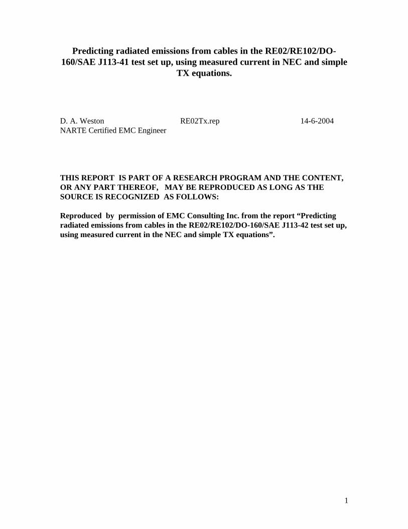
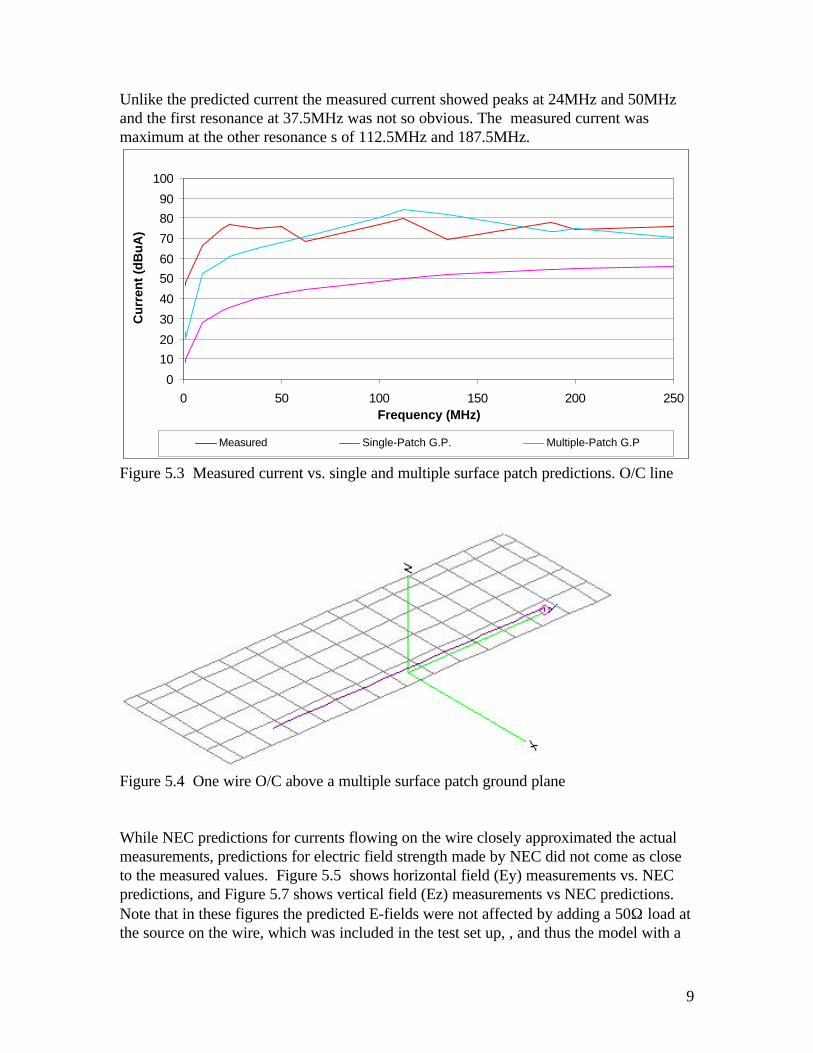
The worst prediction for current resulted from the model using a single surface patchground plane, contrary to what we would expect. Upon modifying the surface patchground plane, such that it was subdivided into multiple smaller patches, the currentprediction improved significantly as shown in figure 5.3. A diagram of the new patchsurface is shown in figure 5.4. The new patch surface consists of 75 patches total. Thelarger patches were square with sides 0.2 m long. Smaller patches were 1/2 to 1/4 of thesize. The wire segment containing the voltage source terminated on the center of a 0.2m x0.2m patch. As noted in the NEC users manual, wires must be terminated at the center ofpatches to produce an accurate model.

9

Unlike the predicted current the measured current showed peaks at 24MHz and 50MHzand the first resonance at 37.5MHz was not so obvious. The measured current wasmaximum at the other resonance s of 112.5MHz and 187.5MHz.

0

10

20

30

40

50

60

70

80

90

100

0 50 100 150 200 250Frequency (MHz)

Cu

rren

t (d

Bu

A)

Measured Single-Patch G.P. Multiple-Patch G.P

Figure 5.3 Measured current vs. single and multiple surface patch predictions. O/C line

Figure 5.4 One wire O/C above a multiple surface patch ground plane

While NEC predictions for currents flowing on the wire closely approximated the actualmeasurements, predictions for electric field strength made by NEC did not come as closeto the measured values. Figure 5.5 shows horizontal field (Ey) measurements vs. NECpredictions, and Figure 5.7 shows vertical field (Ez) measurements vs NEC predictions.Note that in these figures the predicted E-fields were not affected by adding a 50Ω load atthe source on the wire, which was included in the test set up, , and thus the model with a

10

load on the wire over a wire-grid ground plane was omitted from the plots. As shown inthe figures, E-field predictions were affected by subdividing the surface patch groundplane. The multiple-patch ground plane model made a better approximation of themeasured Ey than the single-patch model. Refer to figure 5.6 for a comparison. Theclosest approximation to the measured E-field in the horizontal direction was made by ausing an equation for Ey from the transmission line theory. See appendix 1 for adescription of the transmission line theory.

Ey

0.010.020.030.040.050.060.070.080.090.0

100.0110.0120.0

0 50 100 150 200 250

Frequency (MHz)

E-F

ield

(d

Bu

V/m

)

Measured Tx Line Theory 2 Wire Tx line Infinite G.P.Loaded, Infinite G.P. Wire G.P. Single-Patch G.P. Multiple-Patch G.P.

Figure 5.5 Comparison of the predicted vs the measured electric fields in the horizontaldirection. O/C line

Ey

70.0

80.0

90.0

100.0

110.0

0 50 100 150 200 250

Frequency (MHz)

E-F

ield

(d

Bu

V/m

)

Measured Single-Patch G.P. Multiple-Patch G.P.

Figure 5.6 Comparison of the measured Ey vs single and multiple-patch model predictionsfor the O/C line.

11

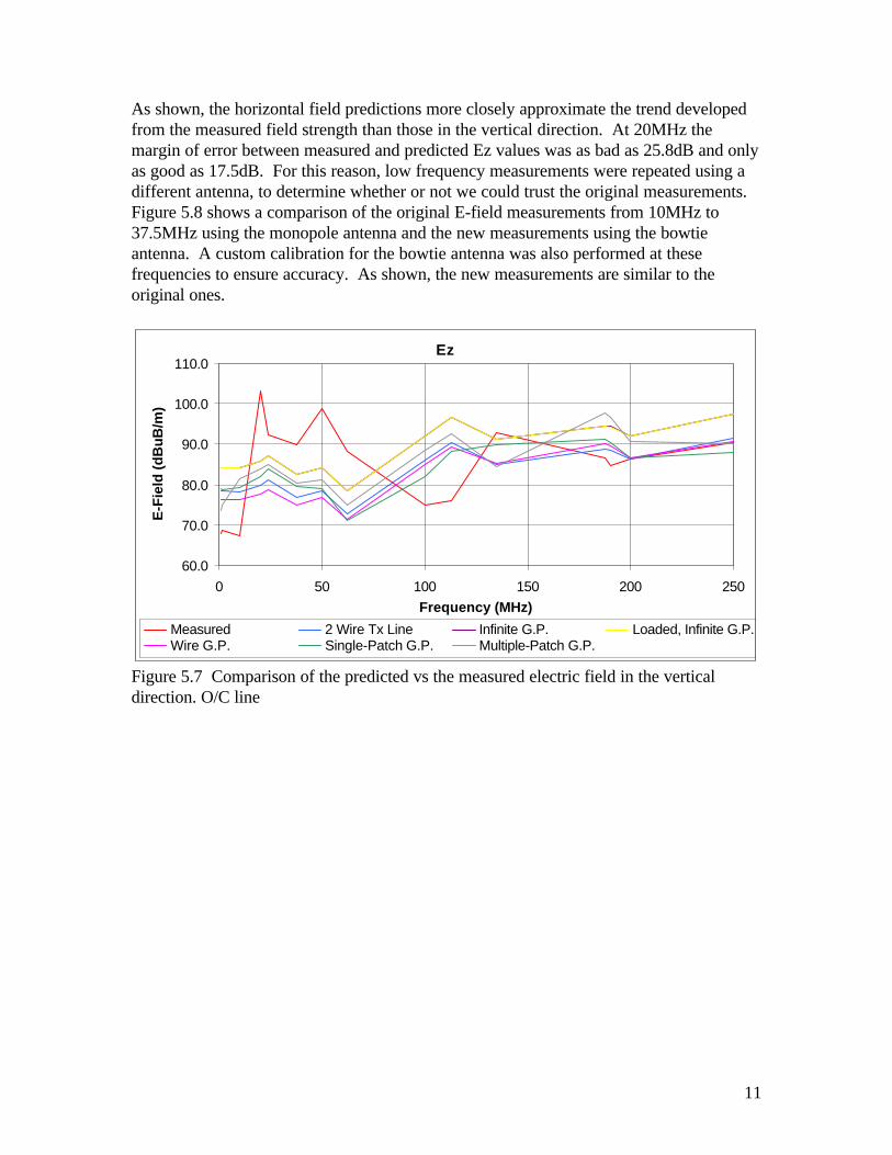
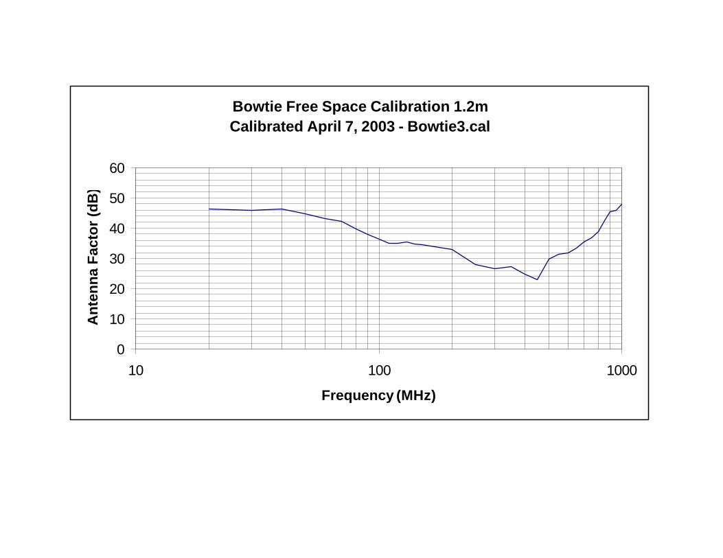
As shown, the horizontal field predictions more closely approximate the trend developedfrom the measured field strength than those in the vertical direction. At 20MHz themargin of error between measured and predicted Ez values was as bad as 25.8dB and onlyas good as 17.5dB. For this reason, low frequency measurements were repeated using adifferent antenna, to determine whether or not we could trust the original measurements.Figure 5.8 shows a comparison of the original E-field measurements from 10MHz to37.5MHz using the monopole antenna and the new measurements using the bowtieantenna. A custom calibration for the bowtie antenna was also performed at thesefrequencies to ensure accuracy. As shown, the new measurements are similar to theoriginal ones.

Ez

60.0

70.0

80.0

90.0

100.0

110.0

0 50 100 150 200 250

Frequency (MHz)

E-F

ield

(d

Bu

B/m

)

Measured 2 Wire Tx Line Infinite G.P. Loaded, Infinite G.P.Wire G.P. Single-Patch G.P. Multiple-Patch G.P.

Figure 5.7 Comparison of the predicted vs the measured electric field in the verticaldirection. O/C line

12

0

20

40

60

80

100

120

10 20 30 40Frequency (MHz)

Ez

(dB

uV

/m)

1m Monopole Bowtie

Figure 5.8 Comparison of O/C RE02 Tx line measurements taken using 1m monopole vs.bowtie antenna

To attempt an explanation of this discrepancy between measured and predicted E-fields,an equation was written to approximate the displacement currents flowing from the braidwire to the ground plane . We find fields calculated based on this model similar to thosepredicted by NEC, and as a result we suspected that the anomalies in the measured datacould be due to resonances in the damped chamber. To test this hypothesis we moved thetest setup outside and repeated the same measurements on the open area test site (OATS).

5.4 O/C Test on OATS

The test setup was identical to that inside the damped chamber/shielded room, except thatthe antenna was placed outside of the fiberglass hut and connected to a long microwavecable running underground to the lab. When using the monopole antenna a coupling planecould not be extended to the ground plane because of the hut wall. Electric field strengthsmeasured were corrected by adding both antenna factors and cable attenuation. SeeAppendix 2 for calibration data. Tables 3 and 4 show current probe and electric fieldstrength measurement data respectively. Figures 5.9 and 5.10, respectively, showcomparisons of the horizontal and vertical e-field measurements taken on the OATS vsthose taken inside the shielded room. OATS E-field measurements were normalized forequal input current to that measured in the room. Resonances and anti-resonances fromthe damped chamber/shielded room appear as peaks and dips on the plots of room Ey andEz measurements. It can be seen that the first resonance resulting in the highest E field andcorresponding to the highest current flow is at 37.5MHz on the OATS, as predicted,however in the chamber measurements the E field peaks at 24MHz and 50MHz and theseare clearly room resonances. A bow tie antenna was used to measures the field at alllocations within the room and the field did not vary significantly from close to the table,

14

200 72.9 9.4 1.6 83.9 76.6 9.4 1.6 87.6250 83.2 10.5 1.9 95.6 72 10.5 1.9 84.4

* measurement made using FET buffer

Ey

0.0

20.0

40.0

60.0

80.0

100.0

120.0

0 50 100 150 200 250 300

Frequency (MHz)

Fie

ld (

dB

uV

/m)

Shielded Room OATS

Figure 5.9 Ey measurements on OATS vs in the Shielded Room. O/C line

Ez

0.0

20.0

40.0

60.0

80.0

100.0

120.0

0 50 100 150 200 250 300

Frequency (MHz)

Fie

ld (

dB

uV

/m)

Shielded Room OATS

Figure 5.10 Ez measurements on OATS vs in the Shielded Room. O/C line

15

Comparisons of the OATS measurements with NEC predictions are shown in figures 5.11and 5.12. In the Y direction OATS measurements lie in the middle of the differing NECpredictions with the infinite ground plane and the wire ground plane models the closest .Again the Tx line theory seems to make the most accurate prediction of the measuredresults in the Ey direction. Z direction E-field measurements on the OATS correlatedmore closely with the NEC predictions, especially at 37.5MHz, than those in the dampedchamber/shielded room , however the differences in the trend still remain and may beconsidered too large to be useful in an EMC evaluation. The main reason for thedifference is that although the current on the cable was maximum at the resonantfrequencies of 37.5MHz, 112.5MHz and 187.5MHz the Ez field was maximum at only37.5MHz and was low at 112.5MHz and 187.5MHz. The field was increasing at 250MHzand may have peaked at the 262.5MHz resonant frequency.

Ey

0.010.020.030.040.050.060.070.080.090.0

100.0110.0120.0

0 50 100 150 200 250

Frequency (MHz)

E-F

ield

(d

Bu

V/m

)

OATS Measurements Tx Line Theory 2 Wire Tx lineInfinite G.P. Loaded, Infinite G.P. Wire G.P.Single-Patch G.P. Multiple-Patch G.P.

Figure 5.11 Ey measurements made on the OATS vs nec predictions. O/C line

16

Ez

60.0

70.0

80.0

90.0

100.0

0 50 100 150 200 250

Frequency (MHz)

E-F

ield

(d

Bu

B/m

)

OATS Measurments 2 Wire Tx Line Infinite G.P. Loaded, Infinite G.P.Wire G.P. Single-Patch G.P. Multiple-Patch G.P.

Figure 5.12 Ez measurements made on OATS vs NEC predictions. O/C line

6) Short Circuit Radiated and conducted test set up and measurements

6.1 Test Procedure

Equipment and procedure for S/C tests was identical to that for the OATS O/C testdescribed above in sections 5.1 and 5.4 with the following exceptions. A brass plate,10cm high and 20cm wide, was soldered to the end of the braid wire and clamped to theground plane. This brass plate ensures a low impedance connection to the ground planeand approximates the wall of an EUT. The antennas used were again the 1m monopolefor 1-24MHz, with an FET buffer for 1.0 and 1.2MHz, and a log-periodic biconicalantenna for 37.5MHz to 250MHz. See figure 6.1 for a diagram of the setup.Measurements for currents and electric fields were conducted in the same fashion used inthe O/C test except that the frequencies 75MHz and 150MHz were added.

17

Marconi 2018A

S/A

1.0m

Antenna: 1m Monopole 1 - 24MHz Log Per. Biconical 37.5 - 250MHz

2m Braid WireFisher

Current Probe

50Ω Resistor

Braid

Clamp

.

.

Ground Plane

5cm

10cm

styrofoam

Fiberglass Hut Wall

styrofoam styrofoam

Brass Plate

Clamp

Figure 6.1 Test set up for S/C test

6.2 Test Results and Calculations

Currents and electric fields were calculated as described in section 5.2. See table 3 forCurrent probe measurement data and table 4 for E-field measurement data taken duringthe S/C test.

Table 3

18

Current Probe Measurement Data for S/C Test. S/C linef

(MHz)Data

(dBuV)Current Probe

Zt (dBW)I

(dBuA)

1 89.5 6.5 831.2 90.1 7.2 82.910 92.6 14 78.620 87 14.6 72.424 84.5 14.6 69.9

37.5 52.6 15.2 37.450 84.1 15.5 68.6

62.3 92.3 15.2 77.175 84.5 15.5 69100 66.3 14.9 51.4

112.5 91.3 15 76.3134.9 71.5 14.8 56.7150 67.6 14.3 53.3

187.5 82 14 68190 83.5 13.8 69.7200 97.6 13.3 84.3250 96.3 11.5 84.8

Table 4E-Field Measurement Data for S/C Test. S/C lineAntenna Vertical Antenna Horizontal

f(MHz)

Data(dBuV)

AF(dB)

CableAtten.(dB)

Total Ez(dBuV/m)

Data(dBuV)

AF(dB)

CableAtten.(dB)

Total Ey(dBuV/m)

1 50.4 9.5 0.6 59.91.2 54.1 10.6 0.6 64.710 35.7 37.4 0.6 73.120 52.6 28.4 0.6 8124 56 24.9 0.6 80.9

37.5 49.5 20.3 0.6 69.8 60.7 20.3 0.6 8150 50.1 17.8 0.6 67.9 68.8 17.8 0.6 86.6

62.3 78.5 14.5 0.7 93 75.1 14.5 0.7 89.675 82.9 9.3 0.9 92.2 59.8 9.3 0.9 69.1100 74.1 9.7 1.2 83.8 72.6 9.7 1.2 82.3

112.5 77 10 1.2 87.0 73.5 10 1.2 83.5134.9 74.1 12.8 1.5 86.9 74.1 12.8 1.5 86.9150 71.3 10.7 1.5 82 66.6 10.7 1.5 77.3

187.5 72 9.4 1.6 81.4 79.5 9.4 1.6 88.9190 67.6 9.4 1.6 77 78.2 9.4 1.6 87.6

19

200 79.1 9.4 1.6 88.5 76.6 9.4 1.6 86250 75.1 10.5 1.9 85.6 72.9 10.5 1.9 83.4

6.3 Analysis

The setup as described in section 6.1 was modeled using software to produce threepredictions for currents on the wire and the received E-fields at the antenna. The modelsproduced using NEC were as follows.

-Two wire Tx line, loaded at the source end with 50Ω

-One wire TX line loaded with 50Ω at the source end and S/C at the load end, above a multiple-patch ground plane

-One wire TX line, loaded with 50Ω at the source end and S/C at the load end above a wire-grid ground plane

The infinite ground plane model was not used as explained in section 7.Figure 6.2 shows a plot of the three predictions for current vs the measured current. Theclosest approximation was predicted using the wire-grid ground plane NEC model.Figures 6.3 and 6.4 show the Ey and Ez measurements on the OATS vs nec predictions.The Nec model using a multiple-patch ground plane makes the best prediction of both theEy and Ez measurements for our S/C braid wire.

20

0

10

20

30

40

50

60

70

80

90

100

0 50 100 150 200 250

Frequency (MHz)

I (d

Bµµ

A)

Measured 2 Wire Tx Line Multiple-Patch G.P. Wire-Grid G.P.

Figure 6.2 Measured current on S/C braid wire vs NEC model predictions for current

Ey

0102030405060708090

100110120

0 50 100 150 200 250

Frequency (MHz)

E-F

ield

(d

Bµµ

V/m

)P

redi

cted

Nor

mal

ized

to

Mea

sure

d U

sing

Cur

rent

Measured on OATS 2 Wire Tx Line Multiple-Patch G.P.

Wire-grid G.P. Tx Line Equation

Figure 6.3 Horizontal E-field measurements vs NEC model predictions. S/C line

21

Ez

112.5

37.5

62.3

0102030405060708090

100110120130

0 50 100 150 200 250

Frequency (MHz)

E-F

ield

(d

Bµµ

V/m

)P

redi

cted

Nor

mal

ized

toM

easu

red

Usi

ng C

urre

nt

Measured on OATS 2 Wire Tx Line Multiple-Patch G.P. Wire-grid G.P.

Figure 6.4 Vertical E-field measurements vs NEC model predictions. S/C line

7) NEC predicted emissions

The Numerical Electromagnetic Code used was 4nec2 version 5.3.4 authored inSeptember 2003 by Arie. 4nec2 uses the nec-2 engine, but incorporates a user-friendlyWindows interface. A copy of the software and its users manual can be obtained at thefollowing address. http://www.qsl.net/wb6tpu/swindex.html

NEC allows a number of methods of modeling the ground plane under the cable and theseare:

• an infinite ground plane

• a ground plane modeled as a patch

• a second wire under the wire cable, which represents the image of the wire in theground plane

• a ground plane made up of a number of wires.

22

The infinite ground plane is suited to generating an electromagnetic image of the wire inthe ground plane and is not suited to predicting current flow in the ground when, forexample, multiple connections of wires to the ground plane are made. For this reason theinfinite ground plane model is omitted from the short circuit transmission line analysis.However as it covers the electromagnetic image of the wire it should be suitable for theopen circuit wire above a ground plane. To find the model which predicted emissionsclosest to the measured, all four configurations were tried for the open circuit prediction.

8) Conclusion

Based on comparisons between measured data and the different NEC models thecorrelation of the vertically polarized field may not be good enough to determine if anEUT will meet RE02/RE102 or similar radiated emission limits based on the measurementof current on the cable. For the prediction of the horizontally polarized field the simpleequations introduced in reference 1 and repeated in Appendix 1 are closer to the measureddata for both short circuited and open circuited lines, and this level of accuracy willtypically be acceptable. The multiple patch ground plane NEC model also provides themost accurate prediction for the Ey field and may also be acceptable in predicting the Ezfields in the short circuited transmission line model.Another large potential source of error are room resonances. Even in our well dampedchamber, resonances at 24MHz and 50MHZ introduce errors when comparing the roommeasurements to the OATS measurements. Many chambers show these TEM modes andalso peaks and nulls in the field due to multiple reflections at higher frequencies, whichare not predominant in our damped chamber/shielded room.A simple equation was developed and used to predict the vertically polarized fieldradiated from the line at 1.0MHz and 1.2MHz. We will try to develop this equation toinclude long line effects and if successful this will be included as an update to this report.This report again validates the simple TX line equation based on radiation resistance andradiated power, by measurements, presented in reference 1 and reproduced in Appendix 1of this report.

23

Appendix 1

Emission from Transmission-Line Geometries (Taken from Reference 1)

To calculate the radiation from a transmission line made up of either two cables or a cableabove a ground plane, use is made of the concept of the radiation resistance of the line.Radiation resistance of an antenna or transmission line is used to describe that part of theconductor resistance that converts a fraction of the power delivered to the load intoradiated power. In an efficient antenna, the radiation resistance is designed to be high andthe resistance, which converts the input power into heat, is low. In the transmission line,the opposite is true. The radiation resistance for a resonant section of two-wire line lengthor λ/2 (or integral multiples of λ/2 when the line is short-circuited (symmetricalconnection), or λ/4 and other multiples when the line is open circuited as in:

l = (2k + 1) λ 4

where k = 0, 1, 2, 3, . . .

when the line is open-circuited or terminated in a load higher than Zc (asymmetricalconnection) or short circuited at both ends (symmetrical connection) then the radiationresistance is,

30β2b2

where b is either the distance between the two-conductor line or twice the height of thecable above a ground plane. The radiated power for the resonant line is given by

30β2b2I2

where I is the current flow on the line, either measured or calculated. For the majority ofEMI conditions, the radiated noise covers a wide range of frequencies, and resonant lineconditions can be expected. For example, when the source of current is converter ordigital logic noise, the harmonics may range from kilohertz up to 500MHz.

The magnetic field some distance R from the line is

H = _ Pk__ 4πR2Zw

where

P = radiated powerZw = wave impedance

24

k = directivity, which is approximately 1.5 for a current loop resonant line and 1.0 for a nonresonant lineR = distance in meters

and the electric field is

E = ZwPk 4πR2

In the near field, the wave impedance is close to the characteristic impedance Zc ofthe transmission line, which may be calculated from

Zc = (Zi + jωle)ωle jk2

where

Zi = distributed series resistance of the two wire line [Ω/m]k = ω µ0e0 = 2π

λle = µ0 ln 2h π a

µ0 = 4π x 10-7 [H/m]

a = diameter of wire [m]

The wave impedance then changes linearly until the near-field/far-field interface, at whichZw = 377Ω. The E field radiated by the current loop may be obtained from E = H x Zw.The equation for calculating the wave impedance in the near field is

Zw = λ/2π - R (Zc - 377) + 377 (Zw < 377 Ω)λ/2π

where R is the distance from the radiation source, in meters.

28

Frequency (kHz) Zt (dBΩΩ)90 -11.6100 -10.7125 -8.8150 -7.2175 -6.0200 -5.0225 -4.1250 -3.5275 -2.5300 -1.6350 -0.3400 0.6450 1.5500 2.2550 2.8600 3.1650 3.7700 4.0750 4.7800 5.0850 5.3900 5.6950 5.9

1000 6.51200 7.21400 8.11600 9.01800 9.32000 10.02500 10.63000 11.23500 11.84000 12.14500 12.55000 12.85500 12.86000 13.16500 13.17000 13.17500 13.48000 13.48500 13.4

29

Frequency (kHz) Zt (dBΩΩ)9000 13.49500 14.010000 14.015000 14.320000 14.625000 14.630000 14.935000 15.240000 15.245000 15.250000 15.560000 15.270000 15.380000 15.690000 15.3

100000 14.9125000 15.2150000 14.3175000 14.6200000 13.3210000 12.4225000 12.0235000 12.1250000 11.5

Mono03U.cal

Fisher Model No. F-33-1 S/N 115 Current Probe CalibrationMar 8, 2004

-100

-80

-60

-40

-20

0

20

40

0.01 0.1 1 10 100 1000 10000 100000 1000000

Frequency (kHz)

Zt

(dB

W)

Mono03U.cal

9.0 8.44E-05 37.39.25 2.08E-04 33.59.5 2.19E-04 33.4

10.0 9.16E-05 37.410.5 3.78E-04 31.411.0 4.66E-04 30.711.5 4.87E-04 30.712.0 5.64E-04 30.312.5 6.22E-04 30.013.0 6.70E-04 29.913.5 6.95E-04 29.914.0 6.89E-04 30.114.5 6.73E-04 30.315.0 6.21E-04 30.815.5 4.76E-04 32.116.0 3.17E-04 34.016.5 3.02E-04 34.417.0 5.04E-04 32.317.5 6.73E-04 31.118.0 9.60E-04 29.718.5 1.01E-03 29.619.0 1.15E-03 29.219.5 1.28E-03 28.820.0 1.44E-03 28.420.5 1.54E-03 28.221.0 1.69E-03 27.921.5 1.90E-03 27.522.0 2.16E-03 27.122.5 2.42E-03 26.723.0 2.81E-03 26.123.5 3.26E-03 25.624.0 3.86E-03 24.924.5 5.02E-03 23.925.0 1.12E-02 20.525.5 1.14E-02 20.526.0 1.73E-02 18.826.5 1.60E-02 19.227.0 1.10E-02 20.927.5 7.97E-03 22.428.0 6.15E-03 23.628.5 5.27E-03 24.329.0 5.36E-03 24.329.5 4.48E-03 25.230.0 4.26E-03 25.5

Mono03U.cal

1m Monopole Calibration at 1m in the Shielded RoomUncoupled, With FET Buffer

August 8, 2003

Frequency (MHz) Antenna Factor (dB)0.01 4.70.02 2.30.03 0.40.04 -1.40.05 -4.30.06 -8.50.07 -9.20.08 -5.70.09 -3.30.1 -2.20.2 2.80.3 4.50.4 5.60.5 6.70.6 7.60.7 8.30.8 8.90.9 9.41.0 9.51.1 10.21.2 10.61.3 11.11.4 11.41.5 11.21.6 11.91.7 11.91.8 12.21.9 12.42.0 12.72.5 13.63.0 14.53.5 14.84.0 15.24.5 15.55.0 15.75.5 16.16.0 16.16.5 14.6

6.91 9.67.0 11.6

7.34 28.67.5 27.58.0 28.7

Mono03U.cal

8.5 17.49.0 14.29.5 16.9

10.0 11.010.5 18.810.8 29.911.0 26.511.5 23.212.0 22.512.5 22.013.0 22.113.5 22.614.0 23.914.5 25.815.0 29.115.5 34.615.7 26.616.0 30.616.5 24.917.0 24.517.5 24.418.0 25.218.5 24.619.0 24.819.5 24.820.0 24.9

Mono03U.cal

1m Monopole Calibration at 1m in the Shielded RoomUncoupled With and Without FET Buffer

August 8, 2003

-20

-10

0

10

20

30

40

50

60

70

0.01 0.1 1 10 100

Frequency (MHz)

An

ten

na

Fac

tor

(dB

)

Buffered Unbuffered

Mono03C.cal

1m Monopole Calibration at 1m in the Shielded RoomCoupled, Without FET Buffer

August 8, 2003

Frequency (MHz) Gain (num) Antenna Factor (dB)0.01 6.12E-08 39.10.02 5.93E-08 42.30.03 6.01E-08 44.00.04 5.81E-08 45.40.05 5.63E-08 46.50.06 5.43E-08 47.40.07 4.92E-08 48.50.08 4.52E-08 49.50.09 3.68E-08 50.90.1 3.33E-08 51.8

0.134 2.69E-08 54.00.2 7.90E-08 51.00.3 2.18E-08 48.40.4 4.21E-07 46.80.5 6.54E-07 45.80.6 9.66E-07 44.90.7 1.31E-06 44.30.8 1.72E-06 43.70.9 2.17E-06 43.21.0 2.67E-06 42.71.1 3.30E-06 42.21.2 3.99E-06 41.81.3 4.63E-06 41.51.4 5.60E-06 41.01.5 5.93E-06 41.01.6 6.47E-06 40.91.7 7.28E-06 40.71.8 8.26E-06 40.41.9 9.45E-06 40.02.0 1.07E-05 39.72.5 1.66E-05 38.83.0 2.51E-05 37.83.5 3.40E-05 37.14.0 4.46E-05 36.54.5 5.50E-05 36.15.0 6.47E-05 35.95.5 7.54E-05 35.66.0 8.61E-05 35.46.5 9.33E-05 35.47.0 9.70E-05 35.67.5 9.48E-05 36.08.0 8.91E-05 36.5

Mono03C.cal

8.5 8.74E-05 36.99.0 1.45E-04 34.99.5 4.84E-04 29.9

9.59 5.23E-04 29.610.0 2.49E-04 33.0

10.31 1.53E-04 35.310.5 2.28E-04 33.611.0 7.30E-04 28.811.5 7.20E-04 29.012.0 6.70E-04 29.512.5 5.74E-04 30.413.0 5.08E-04 31.113.5 4.70E-04 31.614.0 4.15E-04 32.314.5 3.92E-04 32.715.0 3.87E-03 32.915.5 3.69E-04 33.216.0 3.64E-04 33.416.5 1.56E-04 37.216.6 9.59E-04 39.417.0 4.39E-04 32.917.5 5.89E-04 31.718.0 6.41E-04 31.518.5 7.06E-04 31.219.0 7.68E-04 30.919.5 8.55E-04 30.620.0 9.29E-04 30.320.5 1.08E-03 29.821.0 1.23E-03 29.321.5 1.43E-03 28.822.0 1.60E-03 28.422.5 1.88E-03 27.823.0 2.26E-03 27.123.5 2.62E-03 26.524.0 3.00E-03 26.024.5 3.64E-03 25.325.0 4.41E-03 24.525.5 5.17E-03 23.926.0 6.05E-03 23.326.5 7.25E-03 22.627.0 8.57E-03 22.027.5 1.03E-02 21.328.0 1.27E-02 20.428.5 1.48E-02 19.829.0 1.72E-02 19.329.5 2.03E-02 18.630.0 2.29E-02 18.2

Mono03C.cal

1m Monopole Calibration at 1m in the Shielded RoomCoupled, With FET Buffer

August 8, 2003

Frequency (MHz) Antenna Factor (dB)0.01 13.50.02 10.50.03 8.50.04 7.10.05 6.00.06 5.00.07 3.90.08 3.00.09 1.60.1 1.00.2 1.10.3 4.10.4 5.40.5 6.20.6 7.10.7 7.80.8 8.10.9 8.91.0 9.31.1 9.81.2 10.31.3 10.61.4 10.81.5 10.71.6 10.81.7 11.11.8 11.41.9 11.72.0 12.02.5 13.03.0 14.03.5 14.94.0 15.54.5 16.25.0 16.95.5 17.46.0 18.26.5 18.87.0 20.07.5 20.88.0 22.18.5 22.4

Mono03C.cal

9.0 18.79.5 16.8

10.0 20.310.41 24.510.5 24.411.0 18.711.5 18.412.0 20.112.5 21.413.0 22.613.5 24.014.0 24.914.5 26.015.0 27.415.5 29.8

15.95 41.016.0 38.716.5 22.117.0 25.817.5 26.318.0 26.918.5 26.919.0 26.819.5 27.220.0 27.1

Mono03C.cal

1 m Monopole Calibration at 1m in the Shielded RoomCoupled With and Without FET Buffer

August 8, 2003

0

10

20

30

40

50

60

0.01 0.1 1 10 100

Frequency (MHz)

An

ten

na

Fac

tor

(dB

)

Buffered Unbuffered

250.5 5.8211 10.5252.5 5.6555 10.7260.5 5.835 10.9270.5 5.0575 11.8271.5 4.8982 12275.5 4.4607 12.5280.5 3.9285 13.2282.5 3.5508 13.7285.5 2.8868 14.7288.5 2.7162 15.1290.5 2.8345 15291.5 3.0582 14.7293.5 3.4312 14.2295.6 3.9939 13.6297.6 3.8756 13.8299.6 4.1952 13.5300.6 4.5258 13.2305.6 5.1272 12.8310.6 5.8069 12.4311.6 6.0442 12.3323.6 6.2702 12.4325.6 6.3091 12.5330.6 5.9648 12.9335.6 4.8711 13.9339.6 3.9699 14.9340.6 4.2812 14.6345.7 4.6656 14.3349.7 5.0806 14350.7 5.2802 13.9353.7 5.519 13.8355.7 5.7586 13.6357.7 5.5816 13.8360.7 5.0511 14.3368.7 5.7536 14372.7 5.6122 14.2375.7 5.2616 14.5380.7 4.6171 15.2387.7 3.3986 16.7390.7 4.0988 15.9392.7 4.5907 15.5394.7 5.3344 14.9400.8 6.2539 14.3405.8 7.0558 13.9

410.8 6.8925 14.1420.8 6.5742 14.5430.8 5.6113 15.4440.8 5.3401 15.8450.9 4.9069 16.4460.9 4.5015 17470.9 4.433 17.2471.9 4.7766 16.9475.9 4.8172 16.9480.9 4.5273 17.3485.9 4.1053 17.8490.9 4.1476 17.9500.0 4.2238 17.9509.0 4.4562 17.9510.0 4.6272 17.7520.0 4.7019 17.8526.7 4.9415 17.7532.5 4.1696 18.5536.4 2.6255 20.6537.3 2.1953 21.4538.3 1.7071 22.5539.2 1.3774 23.5540.2 1.0711 24.6541.2 1.2856 23.8542.1 1.6591 22.7545.0 2.4784 21550.8 2.4168 21.2555.6 1.7621 22.7556.6 1.5841 23.1560.4 1.3313 23.9561.4 1.4339 23.6565.2 1.6691 23566.2 1.7327 22.9567.1 1.8662 22.6568.1 1.9373 22.4569.1 2.0865 22.1570.0 2.2473 21.8575.8 2.921 20.8580.6 3.5289 20585.4 3.9649 19.6590.2 4.1427 19.5595.0 3.748 20600.8 3.2734 20.6

604.6 3.5422 20.4605.6 3.6767 20.2610.4 3.7102 20.2612.3 3.7219 20.3615.2 3.7394 20.3618.1 3.7526 20.3619.1 3.4995 20.6621.0 3.5104 20.6623.9 3.3992 20.8624.8 3.1699 21.1628.7 3.1894 21.2630.6 3.0834 21.3632.5 3.3255 21635.4 3.592 20.7637.4 4.0146 20.3638.3 3.8753 20.4639.3 4.3297 20640.2 4.6624 19.7644.1 5.2205 19.2645.1 5.6281 18.9648.9 6.0805 18.6650.8 6.7956 18.2656.6 6.8638 18.2660.4 6.896 18.2662.4 6.9241 18.2663.3 6.9262 18.2664.3 7.458 17.9665.3 7.2069 18.1667.2 6.9664 18.3671.0 7.0065 18.3672.0 7.2715 18.2678.7 7.0869 18.3680.6 7.107 18.4683.5 7.1371 18.4690.3 7.2074 18.4700.8 7.3179 18.5705.7 6.8526 18.8710.5 6.4166 19.2720.1 5.8364 19.7730.7 6.5991 19.3740.3 6.9369 19.2750.9 7.036 19.3759.5 6.8676 19.5

760.5 6.6276 19.6769.1 6.468 19.8770.1 6.249 20780.7 6.8036 19.7788.4 6.8707 19.8789.3 6.6379 19.9790.3 6.646 20795.1 6.9373 19.8800.9 6.735 20810.5 6.8158 20.1820.1 6.4142 20.4824.9 6.6863 20.3830.7 6.0424 20.8837.4 5.6718 21.1843.2 5.3113 21.5850.9 4.8045 22853.8 4.6517 22.2861.5 4.6937 22.2862.4 4.5342 22.4865.3 4.3848 22.5870.1 4.7408 22.3900.0 5.0873 22.2909.6 5.7294 21.8945.2 5.9536 22950.9 5.5708 22.3960.6 4.6967 23.2970.2 4.1079 23.8971.1 3.9632 24976.9 3.4524 24.6980.8 3.1105 25.1985.6 2.8051 25.6996.2 2.5444 26.1

1000.0 2.3756 26.5

Bowtie Free Space Calibration 1.2mCalibrated April 7, 2003 - Bowtie3.cal

0

10

20

30

40

50

60

10 100 1000

Frequency (MHz)

An

ten

na

Fac

tor

(dB

)

Shielded Room / OATS Correlation

30

40

50

60

70

80

90

100

110

120

10 100 1000

Frequency (MHz)

Fie

ld (

dB

µµV

)

Shielded Room

OATS

Reference 1 Electromagnetic Compatibility Principles and Applications. Marcel Dekker2001. David A. Weston.