Predicting Multiple Structured Visual Interpretations

Debadeepta Dey Varun Ramakrishna Martial Hebert J. Andrew Bagnell

Carnegie Mellon University

Pittsburgh, PA-15213, USA

{debadeep, vramakri, hebert, dbagnell}@ri.cmu.edu

Abstract

We present a simple approach for producing a small

number of structured visual outputs which have high recall,

for a variety of tasks including monocular pose estimation

and semantic scene segmentation. Current state-of-the-art

approaches learn a single model and modify inference pro-

cedures to produce a small number of diverse predictions.

We take the alternate route of modifying the learning proce-

dure to directly optimize for good, high recall sequences of

structured-output predictors. Our approach introduces no

new parameters, naturally learns diverse predictions and is

not tied to any specific structured learning or inference pro-

cedure. We leverage recent advances in the contextual sub-

modular maximization literature to learn a sequence of pre-

dictors and empirically demonstrate the simplicity and per-

formance of our approach on multiple challenging vision

tasks including achieving state-of-the-art results on multi-

ple predictions for monocular pose-estimation and image

foreground/background segmentation.

1. Introduction

Computer vision tasks such as object recognition [12],

semantic segmentation [4], tracking [18], monocular human

pose estimation [38] and point cloud classification [27], are

often addressed by a pipeline architecture where each mod-

ule of the pipeline produces several hypotheses as input to

the next module. Considering multiple options at each stage

is good practice as it avoids premature commitment to a sin-

gle answer which, if wrong, can jeopardize the quality of

decisions made downstream [10, 37]. As an example con-

sider Figure 1 where multiple predictions are generated for

a foreground/background segmentation task. We see that

the prediction with the highest confidence (denoted by pre-

diction 1) can be far from the groundtruth. The principal

requirement of a list is that at least one hypothesis in the

list is close to the groundtruth labeling (high list recall). A

characteristic of lists which achieve high recall in a small

number of hypotheses is diversity [32] which increases the

odds of at least one accurate prediction.

Image Prediction 1 Prediction 2 Prediction 3

Figure 1: For a given image our method trains a small num-

ber of structured predictors in sequence. For a test image,

the list of predictors are invoked to produce multiple hy-

potheses. Our approach produces high recall lists within a

small number of hypotheses and can use any structured pre-

dictor available.

Such fixed length lists with high recall need to be consid-

ered in many other non-vision tasks including information

retrieval, server job scheduling, document summarization,

grasping and motion planning. For example in information

retrieval, when a user searches for the term “jaguar” on a

search engine, the user may either intend to search for the

animal, the car, or the football team. Search results must

include highly ranked links to all three possible interpreta-

tions [32]. These problems have received much attention

in recent literature [7, 8, 23, 24, 32, 33, 34, 40, 41].

Our central insight is that diversity in a list of structured

predictions need not be enforced, but that it is an emergent

property of optimizing the correct submodular recall objec-

tive. Our procedure trains a sequence of predictors, each of

which produces a hypothesis, which constitutes the list.

Submodular functions are characterized by a diminish-

ing returns property that implies that any list that maximizes

a monotone submodular function will implicitly produce di-

verse hypotheses. This is due to the fact that adding hy-

potheses which are similar to previously chosen hypotheses

in the list results in small marginal gains. For example, in

the semantic scene labeling problem it is not beneficial to

predict a labeling in the second position of the list which

differs from the first labeling in the list only by a few pix-

els. Note that the desired property is to achieve high recall,

while diversity is merely a characteristic of lists that achieve

12947

this. Therefore our objective optimizes for recall and does

not explicitly enforce diversity, instead the maximization

of the submodular objective naturally produces diverse hy-

potheses. Conveniently, submodular monotone functions

can be maximized efficiently by greedily maximizing the

marginal benefit which ensures performance within 1 − 1e

(∼ 63%) of the optimal list of items of a fixed length [28].

Since monotone submodular functions exhibit this dimin-

ishing returns property as the list of input arguments grows,

they have been harnessed to serve as convenient objective

functions for optimizing both low-error items and diver-

sity [7, 24, 32, 40].

The vision tasks mentioned above are generally posed as

structured prediction problems. Making a single best pre-

diction in structured problems is difficult due to the combi-

natorially large state space that has to be considered. While

a number of approaches, both probabilistic [19, 22] and

margin-based [35, 36], for learning and inference in struc-

tured problems are well known, methods for making multi-

ple predictions in structured problem domains are relatively

few [2, 14, 20, 30]. We develop a learning-based approach

to produce a small list of structured predictions that ensures

high recall in a variety of computer vision tasks.

In contrast to recent developments which train a sin-

gle model during the learning phase and modify the infer-

ence procedure to produce multiple hypotheses at test time

[2, 20, 30], our approach trains separate predictors during

the learning phase to produce each of the hypotheses in the

list. This alternate approach has several advantages—the

learning procedure is optimized for the task of producing a

list with high recall; diversity does not need to be enforced

in an ad hoc fashion but is an emergent property of lists

that maximize our objective; it is agnostic to the inference

method used and can be utilized for any class of structured

predictor. The primary contributions of our approach are:

• Our approach is a model agnostic framework applicable

to extending any structured prediction algorithm to make

multiple predictions. In any task domain for which learn-

ing algorithms exist to generate a single best prediction,

our approach can be employed for making multiple pre-

dictions by training multiple instances.

• Our approach is parameter free. In contrast, current state-

of-the-art approaches enforce diversity by explicitly in-

troducing a diversity modeling term in the objective func-

tion. Such parameters are tuned on validation data. It is

not clear that artificially enforcing diversity in such a way

is the right thing for the task at hand to achieve the best

performance [5, 26].

• We study the empirical performance of our ap-

proach and demonstrate state-of-the-art results on

multiple predictions for monocular pose estimation

and foreground/background segmentation on benchmark

datasets.

2. Related Work

Significant prior work exists in the non-structured out-

put domain. Dey et al. [7] leveraged the work of Streeter

and Golovin [34] and proposed a reduction of list predic-

tion to training a list of classifiers or regressors (Contex-

tual Sequence Optimization – CONSEQOPT). This allowed

the approximate greedy procedure proposed by Streeter and

Golovin [34] (independently discovered by Radlinski et

al. [32]) to be used with features of the task environment.

Ross et al. [33] extended [34] and CONSEQOPT to predict

lists by training a single predictor instead of a list of predic-

tors. This procedure makes the training step more data effi-

cient. Kulesza et al. [21] have adapted determinantal point

processes (DPP), a model used in particle physics for opti-

mizing for diverse but low error predictions. DPPs are espe-

cially attractive because they allow for efficient, exact infer-

ence procedures and are similar to submodular optimization

methods.

The related work in multiple structured prediction can be

grouped into two categories: 1) The first are methods which

are model-dependent. These methods are tied to the specific

learning and inference procedure being used (e.g. S-SVM,

CRF) and cannot easily be adapted to different structured

prediction methods. 2) The second category of models are

model-agnostic, which are not tied to the specifics of the

chosen structured prediction method.

Model-dependent methods: Batra et al. [2] deal with the

problem of inferring low error and diverse solutions from

a Markov Random Field (MRF). They approach this prob-

lem by introducing a constraint in the MRF objective func-

tion which says that a new solution must be at least some

distance away from each of the previous solutions. The

constraint is moved to the objective by a Lagrangian mul-

tiplier λ and then solved using a supergradient algorithm.

λ is treated as a free parameter and is optimized over a

validation set. They term this approach as DIVMBEST.

Note that a single model is initially learnt (the MRF) and

only during inference time diverse solutions are obtained

by imposing constraints on the inference procedure. Nilson

et al. [29] and Weiss et al. [39] propose methods for us-

ing loopy belief propagation for finding the most probably

solutions at inference time in graphical models. But their

methods don’t try to incorporate diversity to improve per-

formance. Park and Ramanan [30] use a modified version

of standard max-product inference which aims to enforce

diversity by incorporating part-overlap constraints, which

they term as NBEST.

In the approach proposed by Guzman-Rivera et al. [14],

a structured SVM [36] (S-SVM) is trained for each posi-

tion of the list. During inference time, each S-SVM is

invoked to predict a structured output. They minimize

an upper bound of the non-convex, structured hinge loss

via a kmeans-based initialization step and an expectation-

maximization (EM) style coordinate-descent minimization

2948

algorithm. They term their approach as Multiple Choice

Learning (MCL). In more recent work, Guzman-Rivera et

al. [15] explicitly add diversity to the MCL objective and

optimize a surrogate via an EM style block coordinate-

descent minimization routine similar to MCL. An extra pa-

rameter which trades off between diversity and accuracy is

then tuned via cross-validation. They term this approach as

Diverse Multiple Choice Learning (DivMCL).

In comparison to such model-dependent methods, our

proposed method is model-agnostic and can use any struc-

tured prediction approach.

Model-agnostic methods: To the best of our knowledge,

the only such method is the ad hoc boosting-like weight-

ing scheme used in [14, 16] which we denote henceforth as

GR14. The weighting scheme of GR14 [16] has been used

for specific task of camera re-localization. This method has

a free parameter which must be tuned on validation data.

In comparison our approach is parameter free and achieves

comparable or better results on standard vision tasks.

3. Background: Submodular Functions

The operator ⊕ denotes order dependent concatenation

of lists and V denotes the space of all possible items which

can be used for constructing lists. A function which takes a

list of items as input f : S → [0, 1] is monotone, submod-

ular for any sequence S = Ja1, a2 . . . a|S|K ∈ S where S is

the space of all possible lists of items a1...|S| ∈ V , if it satis-

fies two properties. 1). Monotonicity: for any list S1, S2 ∈S , f(S1) ≤ f(S1 ⊕ S2) and f(S2) ≤ f(S1 ⊕ S2) 2). Sub-

modularity: for any list S1, S2 ∈ S , and any particular item

a ∈ V , f(S1⊕S2⊕JaK)−f(S1⊕S2) ≤ f(S1⊕JaK)−f(S1).A simple way of maximizing such a monotone, submodu-

lar function f is by greedily choosing an element a which

maximizes the benefit of adding it to the pre-existing list S,

i.e., a∗ = argmaxa∈A

(f(S ⊕ JaK)− f(S)) where a∗ is the

next element to be added to the list. Nemhauser et al. [28]

proved that for an input list of fixed length, the greedy algo-

rithm achieves at least 1− 1e

of that achieved by the optimum

list of the same length.

4. Predicting Multiple Visual Interpretations

Structured prediction problems in machine learning and

computer vision are characterized by a multidimensional

structured output space Y , where the notion of structure

varies according to the problem. For example, in seman-

tic scene understanding, the structure in the output y ∈ Yrefers to the fact that nearby regions in the image tend to

have correlated semantic labels. In human pose estimation

from images, the location of a limb in the image is corre-

lated with the locations of other limbs.

One possible approach to structured predictions could be

to use the well understood approach of multi-class classifi-

cation by treating each possible structured output as a label.

If this were possible, multiple low error and diverse inter-

pretations could be directly generated using a scheme such

as CONSEQOPT [7]. However, the challenge in such struc-

tured prediction tasks is that the space of possible output

variable combinations is exponential in the number of labels

for each variable. For example for an image with 104 pix-

els and 21 possible labels for each pixel there are (21)(104)

possible labelings. This is also why structured prediction

tasks cannot be addressed by multi-class classification as

the number of classes is exponentially large. As a result,

directly applying a procedure such as CONSEQOPT to gen-

erate multiple interpretations is infeasible.

Our approach is inspired by the ideas set forth in [7, 8,

33]. We define a monotone submodular function over a

sequence of structured predictors and show that a simple

greedy algorithm can be used to train a sequence of such

predictors to produce a set of structured predictions with

high recall. More formally our problem can be stated as

follows.

Problem Statement: The goal of our approach is, given an

input image I ∈ I, to produce a sequence of N structured

outputs Y (I) = Jy1,y2, . . . ,yN K ∈ Y with low error and

high recall. We formulate this as the problem of learning

a sequence of structured predictors S = Jπ1, π2, . . . , πN Kwhere each predictor πi : I → Y, πi ∈ Π, in the sequence

produces the corresponding structured output yi, where Πis a hypothesis class of structured predictors and Y is the

space of structured predictions.

We begin by describing a submodular objective that cap-

tures the notion of low error and high recall. Let us denote

j th training sample as a tuple {(Ij ,yjgt)}j∈1...|D|, where for

each image Ij , the ground truth structured label is denoted

by yjgt. We denote by l : Y × Y → R ∈ [0, 1], a loss

function that measures the disagreement between the pre-

dicted structured output y and the ground truth structured

label ygt. The corresponding function measuring gain is

thus given by g(y,ygt) = 1 − l(y,ygt). We define a se-

quence of structured outputs as:

YS(I) = Jπi(I)Ki∈1...N (1)

We then define the quality function,

f(YS(I),ygt) = maxi∈1,...,N

{g(πi(I),ygt)}, (2)

= 1− mini∈1,...,N

{l(πi(I),ygt)} (3)

that scores the sequence of structured predictions YS(I) by

the score of the best prediction produced by the sequence

of predictors S = Jπ1, π2 . . . , πN K. We note that to max-

imize this scoring function with respect to the sequence of

predictions at least one of the predictions yi in the sequence

needs to be close to the ground truth. In order to learn a se-

quence of predictors that works well across a distribution of

the data, the objective function we would like to optimize is

2949

Algorithm 1 train seqnbest

1: Input: Sequence length N , structured prediction rou-

tine π ∈ Π, dataset D.

2: S = {}, {wj0 = 1}j∈1...|D|

3: for i = 1 to N do

4: πi = train struct predictor(D, wi−1)

5: S ← S ⊕ πi

6: wi = compute marginal weights(S, D)

7: end for

8: Return: S = Jπ1, π2, . . . , πN K

the expected value of the above function over the distribu-

tion of the data D:

F (S,D) = E(I,ygt)∼D [f(YS(I),ygt)] . (4)

The resulting optimization problem is therefore to find

the sequence of predictors S that maximizes the objective

function F in Equation 4 and can be written as follows:

maxS

E(I,ygt)∼D [f(YS(I),ygt)] . (5)

The function F of the form in Equation 4 can be shown to

be a monotone submodular function over lists of input items

as shown in [8] and reproduced in supplementary material

for convenience. The natural approach for submodular op-

timization problems of the form in 5 is to use a greedy al-

gorithm [28]. In each greedy step i, we add the structured

predictor π∗i , that maximizes the marginal benefit as in Sec-

tion 3. For our objective, maximizing the marginal benefit

is written as:

π∗i = argmax

π∈ΠF (Si−1 ⊕ JπK,D)− F (Si−1,D). (6)

Maximizing the marginal benefit, as written above, over the

space of structured predictors by enumeration is difficult,

because there can be uncountably many such predictors. In-

stead, we take the approach of directly training a structured

predictor to maximize the marginal benefit. As we do not

have access to the true distribution of the data, we maxi-

mize the marginal benefit using the empirical distribution

D. We denote the loss lji = l(yji ,y

jgt) as shorthand for the

loss of the ith predictor on the j th training sample. Rewriting

the objective with respect to the empirical data distribution

and in terms of the loss per example we have,

F (Si−1 ⊕ π, D)− F (Si−1, D))

=∑

j∈D

(

min Jlj1, . . . , lji−1K−minJlj1, . . . , l

ji K)

, (7)

=∑

j∈D

max(

min Jlj1, . . . , lji−1K− lji , 0

)

, (8)

=∑

j∈D

max(

ξji−1 − lji , 0)

. (9)

Algorithm 2 compute marginal weights (S,D)

1: Input: Current sequence of trained structured predic-

tors S, Dataset D2: for j = 1 to |D| do

3: l = {}4: for i = 1 to |S| do

5: li = l(πi(Ij),yj

gt)6: l← l ⊕ li7: end for

8: ξ ← min(l)9: if SEQNBEST1 then

10: wj ← ξ11: else if SEQNBEST2 then

12: wj ← ξ3/(

3ξ2 − 3ξ + 1)

13: end if

14: end for

15: Return: w = {w1, w2, . . . , w|D|}

where ξji−1 in 9 is the minimum loss obtained by the se-

quence of i − 1 predictors on j th sample till now. Since

training procedures for structured predictors are usually im-

plemented to minimize loss we rewrite 9 and 6 as:

π∗i = argmax

π∈Π

∑

j∈D

max(

ξji−1 − lji , 0)

(10)

= argminπ∈Π

∑

j∈D

min(

lji − ξji−1, 0)

(11)

Let us denote the per-example desired loss lActual =

min(

lji − ξji−1, 0)

which is the summand in Equation 10.

Consider the relationship of the loss lActual as a function

of the loss of the current predictor lji and the best loss seen

before the current predictor (ξji−1). This is drawn in Figure

2a and denoted by the line lActual. We observe that if a pre-

dictor obtains a loss greater than the previous best, ξji−1 on

an example it does not contribute towards lowering of the

loss defined in Equation 10. Whereas if it achieves loss less

than ξji−1, it lowers the objective by the same amount that

it is less than ξji−1. Optimizing such a loss directly tends to

be difficult as it can require modifications that are specific

to the structured predictor’s training procedure. Instead, we

take the approach of optimizing a tight linear upper bound

of the loss (lSeqNBest1 in Figure 2a) which results in a pro-

cedure that only requires re-weighting the training data and

is model-agnostic. Consider a linear upper bound on lActual

defined by the parameter wji ,

wji l

ji ≥ lActual. (12)

Training a predictor which optimizes the surrogate loss

on the left hand side of 12 is equivalent to training a struc-

tured predictor which weights each data sample with the

weight wji :

2950

lji →

0 ξji−1

1

Loss

Function

-1

0

1LSeqNBest1

LSeqNBest2

LActual

(a)

ξji−1 →

0 0.2 0.5 0.8 1

Weight

0

0.2

0.5

0.8

1LSeqNBest1

LSeqNBest2

(b)

Figure 2: (a) Upper bound relationship between the pro-

posed surrogate loss and the desired actual loss function (b)

Comparison between the proposed weighting schemes as a

function of the best-loss seen so far.

∑

j∈D

wji l

ji ≥

∑

j∈D

min(

lji − ξji−1, 0)

(13)

Note that by setting the weight of each sample to be pro-

portional to the marginal benefit left (wji ∝ ξji−1) we are

minimizing a tight linear upper bound of the actual loss

function we wish to minimize (lActual). This relationship

is indicated by the line lSeqNBest1 in Figure 2b. Our train-

ing procedure might be reminiscent of boosting [11] where

several predictors are combined to produce a single output.

In contrast, our procedure is trained to produce a sequence

of predictors each of which makes a separate prediction in a

sequence of predictions. Additionally we are also optimiz-

ing a completely unrelated loss function.

An alternative tight linear upper bound can be calculated

by minimizing the L2 norm between lActual and a linear loss

function given by wji l

ji . Consider a family of linear upper

bounds of the quality function lActual which has the form

lSeqNBest2 = wji l

ji + b. (14)

Minimizing the L2 distance between lActual and

lSeqNBest2 (See supplementary material for the derivation

details) we obtain the following weighting scheme:

wji =

(ξji−1)3

3(ξji−1)2 − 3ξji−1 + 1

. (15)

The graphical relationship between ξji−1 and the optimal

weight (slope of the line) in lSeqNBest2 is shown in Figure

2a. We see that lSeqNBest1 weights the examples directly

proportional to the previous best loss ξji−1, while lSeqNBest2

tends to aggressively upweight hard samples which have

high best previous loss (ξji−1 > 0.5) and aggressively down-

weights easier examples which have low best previous loss

(ξji−1 < 0.5).

We summarize our algorithm in Algorithm 1. We begin

by assigning a weight of 1 to each training sample in the

dataset. In each iteration i, we train the structured predictor

Image

Output of

Predictor 1

Output of

Predictor 2

Weight for

Predictor 3

= min(0.9, 0.3)

= 0.3

80% error

60% error

= min(0.8, 0.6)

= 0.6

5% error

85% error

= min(0.85, 0.05)

= 0.05

30% error

90% error

Figure 3: Illustration of SEQNBEST training procedure. Con-

sider a toy training dataset of 3 images (chosen from the iCoseg

dataset [1], where the task is to do foreground/background sepa-

ration. The first predictor gets 30% pixel error on the bear image,

while the second predictor gets 90% pixel error. Intuitively, since

the first predictor did well already on this image, we should not

try as hard on this image compared to the elephant image where

none of the 2 predictors did very well. The rule for weighting data

points for training the next predictor is minimum of the error by

the previous predictors and the last column shows this being ap-

plied to this contrived example. Note that the elephant image has

the highest weight since none of the previous predictors did well

on it, while the helicopter one has the lowest weight, since the first

predictor did really well on it.

πi with the dataset D and associated weights for each train-

ing sample w and append it to the sequence of predictors S.

We recompute the weights w using the scheme described

in Algorithm 2. We iterate for the specified N iterations

and return the sequence S = Jπ1, . . . , πN K of structured

predictors. We term this simple but powerful approach as

“Sequential N-Best” or SEQNBEST.

4.1. An Example

As an example, on the task of image segmentation the

required inputs are the number of predictions we want to

make per example N , training dataset D and the structured

prediction procedure for learning and inference π. We ex-

plain the algorithm via a toy dataset of 3 images (See Figure

3), where the task is to perform foreground/background seg-

mentation by marking each pixel with either the foreground

or background label. Assume that we have trained 2 pre-

dictors already, and are calculating the importance (weight)

of each image for the 3rd predictor. The second and third

columns show the performance of the two predictors on

these images. Note that none of the predictors do well on

the image of the elephant, however one of the predictors

does really well on the helicopter. This tells us intuitively,

that training of the third predictor should concentrate more

on the image of the elephant, but not as much on the other

two since at least one of the previous predictors have done

relatively well on it. The last column in the figure shows

2951

the weights for each image which is the minimum of the er-

rors obtained by all previous predictors. This weighting rule

achieves the desired behavior of working harder on exam-

ples which none of the previous predictors have performed

well on.

5. Experiments

We evaluate our methods against both model-dependent

[2, 14, 30] and model-independent methods [16] (See Sec-

tion 2). Note that the weighting scheme of GR14 [16] has

been used for the specific task of camera re-localization

and published results on standardized datasets do not ex-

ist. We make a best effort comparison by reimplementing

their method for standardized tasks.

We demonstrate that using our simple yet powerful

weighting scheme results in better performance than model-

dependent methods and comparable or better performance

for model-agnostic methods with much less computation

due to lack of parameter tuning step.

5.1. Case Study: Human Pose Tracking in Monoc­ular Sequences

In monocular pose estimation the task is to estimate the

2D locations of anatomical landmarks from an image. The

task is challenging due to the large variation in appearance

and configuration of humans in images. Additional chal-

lenges are posed by partial occlusions, self-occlusions, and

foreshortening. A related task is to track the pose of a hu-

man subject through a sequence of frames of video. In

the tracking by detection paradigm of human pose track-

ing, multiple hypothesis poses are generated per frame of

video and then stitched together using a data association al-

gorithm. This avoids making hard commitment to a single

best pose at a frame. As long as the correct pose is present

amongst the multiple hypothesized poses for each frame,

the algorithm can have a chance at picking the correct one

using additional temporal information.

Datasets: We evaluate our method on producing multi-

ple predictions for each image in the PARSE dataset used

introduced by Yang and Ramanan [38] and on the track-

ing datasets introduced in Park and Ramanan [30] named

“lola”, “lola”, “walkstraight” and “baseball”. We use the

same model, code and training set as Yang and Ramanan

[38] and use our two weighting methods to train N models

as detailed in Algorithm 1 to produce 4 models. We use the

same test set used by Yang and Ramanan to compare the

average percentage of correct parts (PCP) of the best pose

as the number of pose hypotheses is increased from 1 to 4.

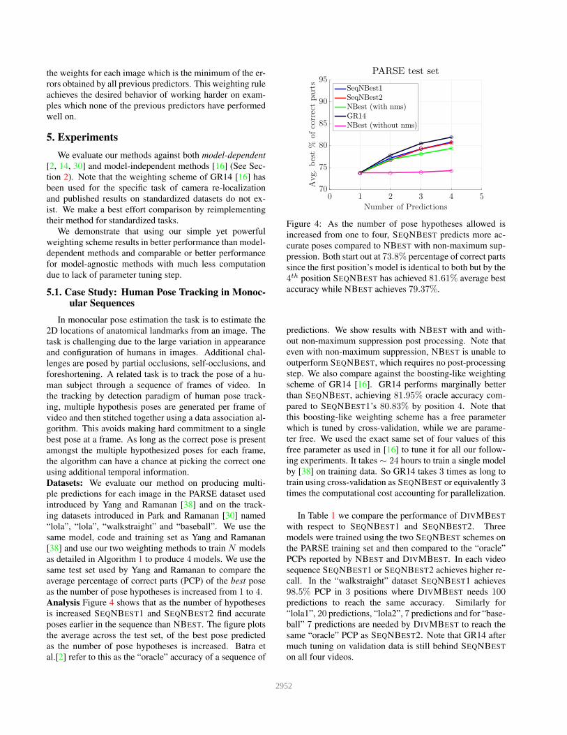
Analysis Figure 4 shows that as the number of hypotheses

is increased SEQNBEST1 and SEQNBEST2 find accurate

poses earlier in the sequence than NBEST. The figure plots

the average across the test set, of the best pose predicted

as the number of pose hypotheses is increased. Batra et

al.[2] refer to this as the “oracle” accuracy of a sequence of

Number of Predictions0 1 2 3 4 5

Avg.

best%

ofcorrectparts

70

75

80

85

90

95PARSE test set

SeqNBest1SeqNBest2NBest (with nms)GR14NBest (without nms)

Figure 4: As the number of pose hypotheses allowed is

increased from one to four, SEQNBEST predicts more ac-

curate poses compared to NBEST with non-maximum sup-

pression. Both start out at 73.8% percentage of correct parts

since the first position’s model is identical to both but by the

4th position SEQNBEST has achieved 81.61% average best

accuracy while NBEST achieves 79.37%.

predictions. We show results with NBEST with and with-

out non-maximum suppression post processing. Note that

even with non-maximum suppression, NBEST is unable to

outperform SEQNBEST, which requires no post-processing

step. We also compare against the boosting-like weighting

scheme of GR14 [16]. GR14 performs marginally better

than SEQNBEST, achieving 81.95% oracle accuracy com-

pared to SEQNBEST1’s 80.83% by position 4. Note that

this boosting-like weighting scheme has a free parameter

which is tuned by cross-validation, while we are parame-

ter free. We used the exact same set of four values of this

free parameter as used in [16] to tune it for all our follow-

ing experiments. It takes ∼ 24 hours to train a single model

by [38] on training data. So GR14 takes 3 times as long to

train using cross-validation as SEQNBEST or equivalently 3times the computational cost accounting for parallelization.

In Table 1 we compare the performance of DIVMBEST

with respect to SEQNBEST1 and SEQNBEST2. Three

models were trained using the two SEQNBEST schemes on

the PARSE training set and then compared to the “oracle”

PCPs reported by NBEST and DIVMBEST. In each video

sequence SEQNBEST1 or SEQNBEST2 achieves higher re-

call. In the “walkstraight” dataset SEQNBEST1 achieves

98.5% PCP in 3 positions where DIVMBEST needs 100predictions to reach the same accuracy. Similarly for

“lola1”, 20 predictions, “lola2”, 7 predictions and for “base-

ball” 7 predictions are needed by DIVMBEST to reach the

same “oracle” PCP as SEQNBEST2. Note that GR14 after

much tuning on validation data is still behind SEQNBEST

on all four videos.

2952

SeqNBest

SeqNBest

SeqNBest

Figure 5: For each of the three images the top row is the sequence of 4 pose hypothesis by NBEST while the bottom 4 are by

SEQNBEST. For baseball player SEQNBEST predicts the correct pose in the 2nd guess, for the gymnast in the 3rd guess and

the 4th guess for the cyclist. Note that in each case SEQNBEST1 produces poses which are diverse from each other while

trying to be relevant to the scene. In each case NBEST produces poses which are almost identical to each other and none of

which are close to the ground truth pose.

Number of Predictions

0 1 2 3Avg.best%

ofcorrectparts

78

80

82

84

86

88

90baseball

SeqNBest1

SeqNBest2

NBest

GR14

DivMBest

Number of Predictions

0 1 2 3Avg.best%

ofcorrectparts

88

90

92

94

96

98

100walkstraight

SeqNBest1

SeqNBest2

NBest

GR14

DivMBest

Number of Predictions

0 1 2 3Avg.best%

ofcorrectparts

50

55

60

65

70

75

80lola1

SeqNBest1

SeqNBest2

NBest

GR14

DivMBest

Number of Predictions

0 1 2 3Avg.best%

ofcorrectparts

45

50

55

60

65

lola2

SeqNBest1

SeqNBest2

NBest

GR14

DivMBest

Table 1: Comparison of SEQNBEST1 and SEQNBEST2 to NBEST and DIVMBEST. The average best PCP plotted as the

budget for generating hypotheses is increased. In each case SEQNBEST1 and/or SEQNBEST2 predicts more accurate poses

for the number of hypotheses allowed.

5.2. Case Study: Image foreground separation

We apply our method to the task of fore-

ground/background segmentation where the task is to

assign each pixel in an image with either the foreground or

background label.

Dataset: We use the set of 166 images of the iCoseg dataset

[1], spanning 9 different events, as used by MCL [14]. The

dataset is roughly, equally split into training, validation and

test sets. The exact splits were provided to us by the authors

of MCL.

Analysis: We compare the performance of SEQNBEST to

MCL in two ways: 1) We use the exact implementation of

S-SVM provided to us by the authors of MCL as the struc-

tured predictor routine in SEQNBEST to train 6 predictors

2) Secondly, to showcase the flexibility of SEQNBEST to

use any structured predictor available, we use the Hierar-

chical Inference Machine (HIM) algorithm by Munoz et

al. [27] to train SEQNBEST. We use texture and C-SIFT

[13] as features. Figure 6 (left) shows the “oracle” accuracy

of a list of predictions. Additionally we compared against

GR14 [16]. We find that using the same predictor and fea-

tures as in MCL, SEQNBEST1 and MCL have comparable

performance in Figure 6 (left). When HIM is used as the

structured predictor (Figure 6 (right)), it performs much bet-

ter from the first position and obtains 6% average best error

in 6 predictions. The reduction of error stops after the first

3 positions because the HIM model starts approaching the

Number of Predictions0 1 2 3 4 5 6 7

Pixel

error%

5

10

15

20

25

30

35FG/BG Segmentation with S-SVM

MCLGR14 (S-SVM)SeqNBest1 (S-SVM)SeqNBest2 (S-SVM)

Number of Predictions0 1 2 3 4 5 6 7

Pixel

error%

0

5

10

15

20

25FG/BG Segmentation with HIM

GR14 (HIM)SeqNBest1 (HIM)SeqNBest2 (HIM)

Figure 6: Average best pixel error in the image background,

foreground segmentation task as number of predictions are

increased. SEQNBEST (with S-SVM) uses the same S-

SVM structured predictor routine as MCL.

theoretical limits of its performance on the test set, which is

2% (this was obtained by training and testing HIM on the

test set itself).

In summary, variants of SEQNBEST performed on par

with model-dependent methods like MCL, which have the

advantage of leveraging the specifics of the chosen struc-

tured predictor (in this case S-SVM). SEQNBEST, how-

ever, is model-agnostic and can be readily applied to any

structured predictor. We find that SEQNBEST used in con-

junction with HIM outperforms the other model-agnostic

method, GR14, which is also trained with HIM as the base

predictor (Figure 6 (right)). This also serves as an exam-

ple of SEQNBEST’s flexibility in being able to plug-in any

powerful predictor.

2953

Table 2: As the number of predictions is increased, we ob-

serve a 10.60% gain in “oracle” accuracy over a single pre-

diction on the PASCAL VOC 2012 val dataset.

Position 1 2 3 4 5

Oracle acc. (%) 42.91 45.96 46.44 47.09 47.46

5.3. Case Study: Image Segmentation

As mentioned earlier semantic scene segmentation is a

very challenging task, where every pixel in an image has to

be assigned a semantic label like “boat”, “sky” etc. In this

section we show initial promising results with SEQNBEST.

Note that these are not meant to be competitive with the

most recent state-of-the-art advances in image segmenta-

tion but meant to showcase the flexibility of our approach

in using any predictor.

Dataset: In PASCAL VOC 2012 segmentation chal-

lenge [9] the task is to mark every test image with one of

20 class labels or the background class. Figure 7 shows

some example images and their annotated groundtruth la-

bels. There are 1464 images in train and 1449 in the val

set which we use as the test set in our experiments below.

Analysis: We use the Hierarchical Inference Machine

(HIM) algorithm by Munoz et al. [27] to learn 5 structured

predictors in the SEQNBEST framework. We use the output

of category-specific regressors of [3] as additional features

to HIM. In the first position HIM achieves 42.91% aver-

age intersection/union accuracy over all 21 classes. Table 2

shows the “oracle” accuracy as the number of predictions is

increased to 5 where the “oracle” accuracy is 47.46% which

is a 10.6% gain.

Prasad et al. [31], have proposed inference procedures

for extracting diverse hypotheses in MRFs using various

higher-order potentials [6]. This is another example of the

model-dependent category of methods as described in Sec-

tion 2. Similar to us, they have demonstrated their method

on the semantic segmentation challenge in PASCAL VOC

2012 val set. They show impressive “oracle” gains of

∽ 12% over a single prediction. Since their model and code

is not yet available, it is not currently possible to directly

compare against SEQNBEST. We use a different model to

achieve similar boosts. Again, this showcases the ease of

use and generality of our approach. Note that we are not

constrained to specific models or specific diversity terms

which may be only compatible with particular model rep-

resentations.

In ongoing experiments we are using recent advances

in convolutional neural networks [17, 25] as the structured

predictor for generating multiple segmentations using SE-

QNBEST.

Figure 7: Qualitative examples of multiple semantic scene

segmentations on the PASCAL VOC 2012 dataset. Each

predictor tries to get right what the previous predictors have

not been able to cover well. For example the cow grazing

scene the first two predictors miss parts of the cow while the

third one gets majority of it correct.

6. Conclusion

We developed and experimentally validated a simple

method for making a high quality sequence of structured

predictions by learning multiple predictors for each slot of

the sequence. The technique presented here directly targets

the problem of interest (a good list of predictions) and is

easily applied in a black box fashion to a very broad set of

structured learners. Moreover, we show it is easily imple-

mented and effective. In contrast to previous methods, we

train multiple models during learning as opposed to mod-

ifying the inference procedure at test time. While this in-

forms the learning process of the eventual task of produc-

ing multiple outputs, it can potentially be inefficient when

training each model is expensive. Future work will consider

the trade-offs and potential combination of learning multi-

ple models and performing multiple rounds of inference for

the problem of producing a good sequence of predictions.

Additionally, our method currently trains the predictor in

each slot by providing the learning procedure with an upper

bound on the marginal benefit for each example. An inter-

esting direction for future work would be to explore meth-

ods for accurately communicating the loss of each possible

labeling during training at each stage in the sequence in a

model-agnostic fashion.

7. Acknowledgements

This work was funded by the Office of Naval Re-

search through the “Provably-Stable Vision-Based Control

of High-Speed Flight through Forests and Urban Environ-

ments” project. We would like to thank Dhruv Batra and

Abner-Guzman Rivera for invaluable help with reproduc-

ing baseline result. Abhinav Shrivastava, Ishan Misra and

David Fouhey for insightful discussions and helping make

the manuscript clearer.

2954

References

[1] D. Batra, A. Kowdle, D. Parikh, J. Luo, and T. Chen. icoseg:

Interactive co-segmentation with intelligent scribble guid-

ance. In CVPR, 2010. 5, 7[2] D. Batra, P. Yadollahpour, A. Guzman-Rivera, and

G. Shakhnarovich. Diverse m-best solutions in markov ran-

dom fields. In ECCV. 2012. 2, 6[3] J. Carreira, R. Caseiro, J. Batista, and C. Sminchisescu. Se-

mantic segmentation with second-order pooling. In ECCV.

2012. 8[4] J. Carreira and C. Sminchisescu. Constrained parametric

min-cuts for automatic object segmentation. In CVPR, 2010.

1[5] R. Caruana, A. Niculescu-Mizil, G. Crew, and A. Ksikes.

Ensemble selection from libraries of models. In ICML, 2004.

2[6] A. Delong, A. Osokin, H. N. Isack, and Y. Boykov. Fast

approximate energy minimization with label costs. IJCV,

2012. 8[7] D. Dey, T. Y. Liu, M. Hebert, and J. A. D. Bagnell. Contex-

tual sequence optimization with application to control library

optimization. In RSS, 2012. 1, 2, 3[8] D. Dey, T. Y. Liu, B. Sofman, and J. A. Bagnell. Efficient

optimization of control libraries. In AAAI, 2012. 1, 3, 4[9] M. Everingham, L. Van Gool, C. K. I. Williams, J. Winn,

and A. Zisserman. The PASCAL Visual Object Classes

Challenge 2012 (VOC2012) Results. http://www.pascal-

network.org/challenges/VOC/voc2012/workshop/index.html.

8[10] P. F. Felzenszwalb and D. A. McAllester. The generalized

A* architecture. JAIR, 2007. 1[11] Y. Freund, R. Schapire, and N. Abe. A short introduction

to boosting. Journal-Japanese Society For Artificial Intelli-

gence, 1999. 5[12] R. Girshick, J. Donahue, T. Darrell, and J. Malik. Rich fea-

ture hierarchies for accurate object detection and semantic

segmentation. In CVPR, 2014. 1[13] S. Gould, O. Russakovsky, I. Goodfellow, P. Baumstarck,

A. Y. Ng, and D. Koller. The stair vision library (v2.4). 2010.

7[14] A. Guzman-Rivera, D. Batra, and P. Kohli. Multiple choice

learning: Learning to produce multiple structured outputs. In

NIPS, 2012. 2, 3, 6, 7[15] A. Guzman-Rivera, P. Kohli, D. Batra, and R. A. Rutenbar.

Efficiently enforcing diversity in multi-output structured pre-

diction. In AISTATS, 2014. 3[16] A. Guzman-Rivera, P. Kohli, B. Glocker, J. Shotton,

T. Sharp, A. Fitzgibbon, and S. Izadi. Multi-output learn-

ing for camera relocalization. In CVPR, 2014. 3, 6, 7[17] B. Hariharan, P. Arbelaez, R. Girshick, and J. Malik. Simul-

taneous detection and segmentation. In ECCV. 2014. 8[18] Z. Kalal, K. Mikolajczyk, and J. Matas. Tracking-learning-

detection. T-PAMI, 2012. 1[19] P. Kohli, A. Osokin, and S. Jegelka. A principled deep ran-

dom field model for image segmentation. In CVPR, 2013.

2[20] A. Kulesza and B. Taskar. Structured determinantal point

processes. In NIPS, 2010. 2[21] A. Kulesza and B. Taskar. Learning determinantal point pro-

cesses. In UAI, 2011. 2

[22] J. Lafferty, A. McCallum, and F. C. Pereira. Conditional ran-

dom fields: Probabilistic models for segmenting and labeling

sequence data. 2001. 2[23] H. Lin and J. Bilmes. Multi-document summarization via

budgeted maximization of submodular functions. In Annual

Conference of the North American Chapter of the Associa-

tion for Computational Linguistics, 2010. 1[24] H. Lin and J. Bilmes. A class of submodular functions for

document summarization. In ACL-HLT, 2011. 1, 2[25] J. Long, E. Shelhamer, and T. Darrell. Fully convolutional

networks for semantic segmentation. CoRR, abs/1411.4038,

2014. 8[26] I. Misra, A. Shrivastava, and M. Hebert. Data-driven exem-

plar model selection. In WACV, 2014. 2[27] D. Munoz, J. A. Bagnell, and M. Hebert. Stacked hierarchi-

cal labeling. In ECCV. 2010. 1, 7, 8[28] G. Nemhauser, L. Wolsey, and M. Fisher. An analysis of

approximations for maximizing submodular set functions I.

Mathematical Programming, 1978. 2, 3, 4[29] D. Nilsson. An efficient algorithm for finding the m

most probable configurations in probabilistic expert systems.

Statistics and Computing, 1998. 2[30] D. Park and D. Ramanan. N-best maximal decoders for part

models. In CVPR, 2011. 2, 6[31] A. Prasad, S. Jegelka, and D. Batra. Submodular meets struc-

tured: Finding diverse subsets in exponentially-large struc-

tured item sets. NIPS, 2014. 8[32] F. Radlinski, R. Kleinberg, and T. Joachims. Learning di-

verse rankings with multi-armed bandits. In ICML, 2008. 1,

2[33] S. Ross, J. Zhou, Y. Yue, D. Dey, and J. A. Bagnell. Learn-

ing policies for contextual submodular prediction. In ICML,

2013. 1, 2, 3[34] M. Streeter and D. Golovin. An online algorithm for maxi-

mizing submodular functions. In NIPS, 2008. 1, 2[35] B. Taskar, C. Guestrin, and D. Koller. Max-margin markov

networks. In NIPS, 2013. 2[36] I. Tsochantaridis, T. Joachims, T. Hofmann, and Y. Altun.

Large margin methods for structured and interdependent out-

put variables. In Journal of Machine Learning Research,

pages 1453–1484, 2005. 2[37] P. Viola and M. Jones. Rapid object detection using a boosted

cascade of simple features. In CVPR, 2001. 1[38] Y. Yang and D. Ramanan. Articulated pose estimation with

flexible mixtures-of-parts. In CVPR, 2011. 1, 6[39] C. Yanover and Y. Weiss. Finding the m most probable con-

figurations using loopy belief propagation. NIPS, 2004. 2[40] Y. Yue and C. Guestrin. Linear submodular bandits and their

application to diversified retrieval. In NIPS, 2011. 1, 2[41] Y. Yue and T. Joachims. Predicting diverse subsets using

structural svms. In ICML, 2008. 1

2955