Predicting low velocity impact damage and Compression-After-Impact(CAI) behaviour of composite laminates

Tan, W., Falzon, B. G., Chiu, L. N. S., & Price, M. (2015). Predicting low velocity impact damage andCompression-After-Impact (CAI) behaviour of composite laminates. Composites Part A: Applied Science andManufacturing, 71, 212-226. https://doi.org/10.1016/j.compositesa.2015.01.025

Published in:Composites Part A: Applied Science and Manufacturing

Document Version:Peer reviewed version

Queen's University Belfast - Research Portal:Link to publication record in Queen's University Belfast Research Portal

Publisher rightsCopyright 2015 Elsevier.This manuscript version is made available under a Creative Commons Attribution-NonCommercial-NoDerivs License(https://creativecommons.org/licenses/by-nc-nd/4.0/), which permits distribution and reproduction for non-commercial purposes, provided theauthor and source are cited.

General rightsCopyright for the publications made accessible via the Queen's University Belfast Research Portal is retained by the author(s) and / or othercopyright owners and it is a condition of accessing these publications that users recognise and abide by the legal requirements associatedwith these rights.

Take down policyThe Research Portal is Queen's institutional repository that provides access to Queen's research output. Every effort has been made toensure that content in the Research Portal does not infringe any person's rights, or applicable UK laws. If you discover content in theResearch Portal that you believe breaches copyright or violates any law, please contact openaccess@qub.ac.uk.

Download date:06. Apr. 2022

Accepted Manuscript

Predicting low velocity impact damage and Compression-After-Impact (CAI)

behaviour of composite laminates

Wei Tan, Brian G. Falzon, Louis N.S. Chiu, Mark Price

PII: S1359-835X(15)00036-6

DOI: http://dx.doi.org/10.1016/j.compositesa.2015.01.025

Reference: JCOMA 3838

To appear in: Composites: Part A

Received Date: 16 April 2014

Revised Date: 19 January 2015

Accepted Date: 20 January 2015

Please cite this article as: Tan, W., Falzon, B.G., Chiu, L.N.S., Price, M., Predicting low velocity impact damage

and Compression-After-Impact (CAI) behaviour of composite laminates, Composites: Part A (2015), doi: http://

dx.doi.org/10.1016/j.compositesa.2015.01.025

This is a PDF file of an unedited manuscript that has been accepted for publication. As a service to our customers

we are providing this early version of the manuscript. The manuscript will undergo copyediting, typesetting, and

review of the resulting proof before it is published in its final form. Please note that during the production process

errors may be discovered which could affect the content, and all legal disclaimers that apply to the journal pertain.

Page 1 of 53

Predicting low velocity impact damage and Compression-After-Impact (CAI) behaviour of composite

laminates

Wei Tan1, Brian G. Falzon1*, Louis N. S. Chiu2, Mark Price1

1 School of Mechanical and Aerospace Engineering, Queen’s University Belfast, Ashby Building, Belfast, BT9

5AH, UK

2 Department of Mechanical and Aerospace Engineering, Monash University, Building 31, Clayton, VIC 3800,

Australia

* b.falzon@qub.ac.uk (B.G. Falzon)

Abstract

Low-velocity impact damage can drastically reduce the residual strength of a composite structure

even when the damage is barely visible. The ability to computationally predict the extent of damage and

Compression-After-Impact (CAI) strength of a composite structure can potentially lead to the exploration of a

larger design space without incurring significant time and cost penalties. A high-fidelity three-dimensional

composite damage model, to predict both low-velocity impact damage and CAI strength of composite

laminates, has been developed and implemented as a user material subroutine in the commercial finite

element package, ABAQUS/Explicit. The intralaminar damage model component accounts for physically-

based tensile and compressive failure mechanisms, of the fibres and matrix, when subjected to a three-

dimensional stress state. Cohesive behaviour was employed to model the interlaminar failure between plies

with a bi-linear traction-separation law for capturing damage onset and subsequent damage evolution. The

virtual tests set up in ABAQUS/Explicit were executed in three steps, one to capture the impact damage, the

second to stabilize the specimen by imposing new boundary conditions required for compression testing and

the third to predict the CAI strength. The observed intralaminar damage features, delamination damage area

as well as residual strength are discussed. It is shown that the predicted results for impact damage and CAI

Page 2 of 53

strength correlated well with experimental testing without the need of model calibration which is often required

with other damage models.

Keywords: B. Impact behaviour, B. Strength, C. Damage mechanics, C. Computational modelling, C.

Numerical analysis, C. Finite element analysis (FEA)

1. Introduction

Composite materials are increasingly being used in aerospace structures due to their high specific

stiffness and strength, corrosion resistance and fatigue performance. Nevertheless, the susceptibility to

damage from low-velocity impact events (e.g. accidental damage incurred during routine maintenance) is a

major concern. When subjected to impact loading, a composite structure is degraded through various failure

mechanisms involving the interaction of matrix cracking, fibre pullout/breakage and delamination. Even with

barely visible impact damage (BVID), strength can be significantly reduced. The accurate assessment of the

influence of impact damage currently requires extensive experimental testing to meet certification

requirements, which is costly and time-consuming. It is therefore essential that a reliable computation tool is

developed to support the certification process for the accurate prediction of impact damage and the

corresponding residual strength.

Various composite damage models have been presented in the literature in recent years, focusing on

the application of continuum damage mechanics (CDM) as proposed by Kachanov [1] and further developed

by Lemaitre and Chaboche [2]. Most of these models are based on capturing the behaviour of unidirectional

pre-impregnated composite plies, reflecting their prevalent use in high-performance applications. Accurately

capturing transverse compressive matrix and longitudinal (fibre-dominated) damage are considered essential

features of a reliable damage model. A number of the computational damage models reported, have adopted

Puck and Shurmann’s [3] phenomenological methodology for determining the initiation of matrix fracture.

Contributions to the characterisation of longitudinal compressive failure were reported by Pinho et al. [4, 5].

Page 3 of 53

Donadon et al.[6] and Falzon et al. [7-9] presented a three dimensional (3D) CDM-based material model to

investigate the progressive intralaminar degradation of composite laminates with non-linear shear behaviour,

ply friction and damage irreversibility taken into account. This model was combined with cohesive elements to

capture interlaminar damage. Raimondo et al. [10] proposed a similar intralaminar model where the matrix

crack orientation, within each finite element, was permitted to assume an orientation parallel to the ply

interfaces to approximate delamination and consequently, interface elements were not used to capture

delamination. This implementation also made use of a crack density parameter instead of a characteristic

length measure for mesh objectivity which, in the absence of appropriate reliable experimental data, is

effectively a calibration parameter. More recently, Bouvet et al. [11] andHongkarnjanakul et al. [12] captured

intralaminar matrix cracking in a 3D finite element mesh using cohesive interface elements through the

thickness of each ply, which in turn was modelled with a single layer of 3D elements. Cohesive elements were

also used to capture delamination.

A number of researchers have published experimental results on CAI of composite laminates. Uda et

al. [13] investigated the failure mechanisms of impact-damaged UT500/Epoxy and AS4/PEEK CFRP laminates

subjected to compression fatigue. Ghelli and Minak [14] conducted CAI tests on thin laminates where

interactions between the extent of impact damage and buckling mode shape were shown to influence the

overall strength of the specimens. CAI tests were also performed to investigate the residual strength of a

composite laminate with a cork thermal shield [15] , assess the effectivenss of self-healing composites in

recovering CAI strength [16] and compare the influence of matrix toughness using thermoset and

thermoplastic resins on CAI behaviour [17].

Compared to the research effort associated with experimental tests, fewer studies have been reported on

both impact and CAI simulation. Davies et al. [18] investigated the CAI strength of composite sandwich panels

where the honeycomb core was simulated using an elasto-plastic material formulation in compression and

shear. González et al. [19] proposed a 3D finite element model with interlaminar and intralaminar damage

using a rigorous thermodynamic framework, for drop-weight impact and CAI test simulations, and studied the

Page 4 of 53

effect of different stacking sequences. Rivallant et al. [20] also presented a finite element model focussing on

the fibre failure and delamination to simulate both impact and residual strength tests, and achieved good

correlation between experimental and numerical results.

The work presented in this paper exploits improvements made to the composite damage model by

Falzon et al. [7-9, 21], which include an improved non-linear shear response and a unified matrix-dominated

damage initiation and mixed-mode intralaminar damage progression, to simulate both impact and compression

after impact. The predictive capabilities of the model are confirmed by validating with experimental results

obtained from the literature without the need for calibrating any of the published experimentally-determined

material parameters from established testing laboratories.

2. Composite damage model

The failure modes exhibited by laminated composites can be broadly classified into intralaminar

(matrix cracks and fibre pullout/breakage) and interlaminar (delamination) damage as shown in Fig. 1.

INSERT: Fig. 1. Damage modes in laminated composites

The effective stresses are defined as stresses transmitted across the intact part of the cross-section in a

Representative Volume Element (RVE). The damage tensor is a function of three monotonically increasing

damage variables, bound by 0 (no damage) and 1 (complete failure), each relating to a form of damage mode

under a different loading state; (i) 11Td refers to tensile damage in the fibre direction, (ii) 11

Cd refers to

compressive damage in the fibre direction and (iii) matd refers to matrix cracking due to a combination of

transverse tension/compression and shear loading, which is a unified matrix damage mechanism and replaces

the previous model presented in [7].

Page 5 of 53

The components of the effective stress tensor, σ�

, and true stress tensor, σ , can be linked by the

damage tensor, D , undamaged material elasticity tensor C and the strain tensor ε ,

ε ,σ σ= =D DC�

(1)

assuming strain equivalence, where

23 32 21 31 23 31 21 32

22 33 22 33 22 33

12 13 32 31 13 32 31 12

11 33 11 33 11 33

13 12 23 23 13 21 12 21

22 11 22 11 22 11

12

23

13

1

Ψ Ψ Ψ

1

Ψ Ψ Ψ

1

Ψ Ψ Ψ

E E E E E E

E E E E E E

E E E E E E

G

G

G

ν ν ν ν ν ν ν ν

ν ν ν ν ν ν ν ν

ν ν ν ν ν ν ν ν

− + +⎡ ⎤⎢ ⎥⎢ ⎥

+ − +⎢ ⎥⎢ ⎥⎢ ⎥⎢ ⎥+ + −=⎢ ⎥⎢ ⎥⎢ ⎥⎢ ⎥⎢ ⎥⎢ ⎥⎣ ⎦

C (2)

and 12 21 23 32 31 13 12 23 31

11 22 33

1 2Ψ

E E E

ν ν ν ν ν ν ν ν ν− − − −= .

In order to maintain a positive definite elasticity tensor, C , the Poisson’s ratios must also be degraded when

damage has initiated according to Eqn. (3). This approach is consistent with the experimentally observed

Poisson’s ratio degradation that accompanies the progression of damage in composite materials [22].

, ,

, ,

(1 ) (1 ), , 1, 2,3

(1 ) (1 )ij d ij ii ji jj ji d

ii d ii ii jj jj jj d

d di j

E E d E d E

ν ν ν ν− −= = = =

− − (3)

To account for irreversibility, the damage variable as a function of analysis time, t, defined as

{ }{ }( ) 0, 1, ( )

, 1, 2,3( ) ( )

ii ii

ii ii

d t t max min d t ti

d t t d t

⎧ + = +⎪ =⎨+ ≥⎪⎩

� �

�

. (4)

Page 6 of 53

2.1 Intralaminar damage model

2.1.1 Fibre-dominated failure modes

A bilinear law (Fig. 2) was used, for simplicity, to model the material response in the fibre direction

where damage is characterised by fibre pullout, fibre-matrix debonding and fibre breakage. The point of

damage initiation was found by comparing the strain to the longitudinal failure initiation strain. Damage

initiation functions were defined for both tensile 11TF and compressive 11

CF loading,

( )2

1111 11

11

1TOTFεεε⎛ ⎞

= ≥⎜ ⎟⎝ ⎠ (5)

( )2

1111 11

11

1COCFεεε⎛ ⎞

= ≥⎜ ⎟⎝ ⎠, (6)

where the failure initiation strains ( 11OTε and 11

OCε for tension and compression, respectively) were determined

by the strengths in the respective directions, i.e. 0

11 11/OT TX Eε = etc. When the initiation function reaches

unity, damage begins to grow and the transmitted stress is gradually reduced to zero,

( )( )( )

( )1111 111T C

T CT C dσ σ= −�

. (7)

INSERT: Fig. 2. Bilinear law (shaded area is volumetric strain energy density ( )

11T Cg )

The area under the traction-separation curve, is the volumetric strain energy density and the damage

parameter associated with a reduction in secant stiffness, under loading in the fibre direction, is given by

Page 7 of 53

( )( ) ( )

( ) 11 1111 11 ( ) ( ) ( )

11 11 11

1 FT C OT C

T CFT C OT C T Cdε εε

ε ε ε⎛ ⎞

= −⎜ ⎟− ⎝ ⎠ (8)

where the same damage parameter was used to degrade the transmitted stress (c.f. Eqn. 11 in [23]). Mesh

objectivity of the model was achieved by employing the crack-band model of Bažant and Oh [24], where a

characteristic length of the finite element (equivalent to a RVE), fibl , and the corresponding fracture

toughness, ( )

11ΓT C

, were used. The failure strain, at which net-section fracture across the element occurs, was

determined by the critical energy release rate, characteristic length and longitudinal strength, ( ) , T CX

( ) ( )

( ) 11 1111 ( ) ( )

2 2Γ

T C T CFT C

T C T Cfib

g

X X lε = = (9)

An accurate measure of the characteristic length is the ratio of the elemental volume V and fracture plane

area A ,

fib

Vl

A= (10)

where A is calculated using an approach proposed in [21] and described in Section 2.1.2.

2.1.2 Matrix failure modes

Matrix failure is characterised by matrix cracking, which could be the result of a combination of

transverse (22), through-thickness (33) and shear stresses (12, 13 and 23). In contrast to the assumptions

made for fibre-dominated failure modes, the transverse response is governed by the orientation of the fracture

plane, which may not necessarily be normal to the loading direction. For tensile loading, this fracture plane will

be normal to the load but as suggested by Puck and Schürmann [3], under compressive and/or shear loading,

the failure plane orientation is determined by the ability of the matrix to withstand shear loading. The damage

initiation and the subsequent progression of damage were calculated on the fracture plane as shown in Fig. 3.

The stress tensor on the fracture plane was rotated using the standard transformation matrix ( ) θT .

Page 8 of 53

( ) ( )123θ [ θ ]TLNT T Tσ σ⎡ ⎤= ⎣ ⎦ (11)

INSERT: Fig. 3. Material coordinate system (123) rotated to the fracture plane

coordinate system (LNT)

Non-linear shear response

The matrix failure initiation criterion is based on the stress state acting on the fracture plane,

assuming a pre-damage linear normal stress NNσ and non-linear shear stresses ( )LN NTτ . In this context, the

non-linear shear stress profiles were defined by a cubic law, obtained using a least square fitting method to

experimental data,

( ) ( )3 21 2 3ij ij ij ij ijc sgn c cτ γ γ γ γ γ= − + (12)

where ci are the corresponding coefficients. Similar to the fibre-dominated damage, the transverse stress

transmitted is linearly degraded by damage. The non-linear shear is expressed as the sum of an elastic and

inelastic component,

, , ij ij el ij in i jγ γ γ= + ≠ . (13)

Prior to damage initiation, shear loading and unloading occurs along gradients defined by the initial shear

modulus ijG , shown by paths 1 and 2 in Fig. 4. When damage is triggered, at 0τ , the response follows a

negative tangent stiffness resulting in the softening of the secant shear modulus, with increasing applied strain,

to (1 )mat ijd G− , shown by path 3. Isotropic hardening was adopted to deal with load reversal.

INSERT: Fig. 4. Non-linear shear curve with different loading/unloading paths

Page 9 of 53

Matrix damage initiation

Puck’s criterion is widely used for predicting matrix-dominated damage behaviour. However, this

criterion does not account for in-situ effects, i.e., where the effective shear strength of a ply may be shown to

increase when embedded in a multidirectional laminate. Moreover, for matrix tensile failure, this criterion

provides reasonable predictions only if certain relations between material strengths are satisfied. For instance,

under pure transverse tension, the criterion provides correct predictions only if 232TY S≤ , where TY is

the transverse tensile strength and 23S is the transverse shear strength. The failure initiation criterion, taking

into account the in-situ effect based on Catalanotti et.al.[25], overcomes this limitation and was adopted in the

damage model.

If the normal stress in the fracture plane is compressive, 0NNσ ≤ , then

( )2 2

12 23 LN NT

is isLN NN NT NN

FS S

τ τθμ σ μ σ

⎛ ⎞ ⎛ ⎞= +⎜ ⎟ ⎜ ⎟− −⎝ ⎠ ⎝ ⎠

(14)

and if the normal stress in the fracture plane, is tensile, 0NNσ >

( )2 2 2 2

23 23 23 23 12 23

NN LN NT NN LN NNis is is is is isF

S S S S S S

σ τ τ σ τ σθ λ κ⎛ ⎞ ⎛ ⎞ ⎛ ⎞ ⎛ ⎞ ⎛ ⎞⎛ ⎞

= + + + +⎜ ⎟⎜ ⎟ ⎜ ⎟ ⎜ ⎟ ⎜ ⎟ ⎜ ⎟⎝ ⎠⎝ ⎠ ⎝ ⎠ ⎝ ⎠ ⎝ ⎠ ⎝ ⎠ (15)

where parameters κ and λ are given by ( ) ( )2 2,

12

,23

is T is

is T is

S Y

S Yκ

−= , 23

12

2 isLN

is

S

S

μλ κ= − ,, T isY is the in-situ

transverse shear strength and 12isS and 23

isS are the in-situ shear strengths. The transverse friction

coefficients, defined in [6], are based on Mohr-Coulomb theory where ( )1

tan 2NT

f

μθ

= − ,

( ),

232 tan

C isis

f

YS

θ= , where

,C isY is the in-situ transverse compressive strength, and 12

23

is

LN NTis

S

Sμ μ= . The

Page 10 of 53

fracture plane orientation, fθ , is typically found to be approximately 53° for unidirectional composites [6]

under uniaxial transverse compressive loading. For a general 3D load state, the orientation is not known a

priori and is determined by the angle which maximizes the failure criteria functions of Eqn (13) or Eqn (14).

Brent’s algorithm [26] was used for this purpose which combines a golden section search with parabolic

interpolation.

Matrix mixed-mode damage propagation

Matrix failure is attributed to loading in transverse compression and shear. Once damage initiates, the

stresses on the fracture plane and the characteristic length are recorded. A single damage parameter, matd ,

was used to define the degradation of the combined stress state, rσ ,

( ) ( )2 22r NN NT NLσ σ σ σ= + + (16)

with corresponding strain, rε , acting on the fracture plane [7, 10], defined as the vector sum of the elastic and

inelastic components, , ,r r el r inε ε ε= + , where

( ) ( )2 22,

el elr el NN NT NLε ε γ γ= + + (17)

( ) ( )2 2

,in in

r in NT NLε γ γ= + (18)

and ( )max 0,x x= is the McCauley operator. Fig. 5 shows the overall damage propagation for mixed-mode

matrix damage where

0 0,0 0

,

fr r in r r

mat fr r r r in

dε ε ε εε ε ε ε

⎛ ⎞− −= ⎜ ⎟− −⎝ ⎠(19)

The shear stresses on the fracture plane are degraded by the matrix damage parameter matd ,

Page 11 of 53

( )1 ,LNLN matdσ σ= −�

( )1 ,NTNT matdσ σ= −�

.NN NNNN matdσ σ σ= −� �

(20)

These stresses are then transformed back to the material coordinate system to form the complete stress

tensor of the damaged element.

The overall shear loading and unloading, prior to damage initiation, (Fig. 5) occurs along gradients defined by

the initial shear modulus rG�

, given by,

0

0,

rr

r el

Gσε

=�

(21)

INSERT: Fig. 5. Mixed-mode matrix damage evolution

The corresponding damage parameter, matd , is assumed to be a function of the resultant strain, 0 , rε at

damage initiation and the failure resultant strain, frε , which is governed by the mixed-mode critical strain

energy release rate, Γr and characteristic length, matl , given in the next section,

C

0r00

2( )f

r rr mat

gl

ε εσ

Γ= − + (22)

The volumetric strain energies, at damage initiation, associated with each stress component on the fracture

plane, are combined using a quadratic relationship, which can be represented by the dashed region in Fig.5,

2 2 20 0 00 0 0

0 0 0 0NN LN NT

NN LN NTr r r

g g g gσ τ τσ σ σ

⎛ ⎞ ⎛ ⎞ ⎛ ⎞= + +⎜ ⎟ ⎜ ⎟ ⎜ ⎟⎝ ⎠ ⎝ ⎠ ⎝ ⎠

(23)

Page 12 of 53

The volumetric strain energy associated with each stress component, 0ig , where i denotes NN , LN and

NT , is given by

0

0

0

i

i i ig dε

σ ε= ∫ . (24)

The critical mixed-mode strain energy release rate, CrΓ , is then given by

2 2 20 0 0Cr 22 12 230 0 0Γ Γ Γ

C C CNN LN NT

r r r

σ τ τσ σ σ

⎛ ⎞ ⎛ ⎞ ⎛ ⎞Γ = + +⎜ ⎟ ⎜ ⎟ ⎜ ⎟⎝ ⎠ ⎝ ⎠ ⎝ ⎠

(25)

where Γ ( 22,12,23)Cij ij = , are the corresponding critical strain energy release rates for each stress

component. The blue area, in Fig.5, is the inelastic strain energy density, ing ,

0 0

, / 2in o r r elg g σ ε= − (26)

Characteristic length calculation

The characteristic length given by ABAQUS is the cubic root of the volume of the element, which is

only accurate when elements have aspect ratios close to unity and crack planes are assumed to evolve

perpendicular to the midplane of the element. Therefore, a much more accurate measure of characteristic

length should be calculated as a function of the crack plane orientation.

INSERT: Fig. 6. Calculation of the characteristic length

The fracture surface is defined by a unit normal vector (�

n ) in an arbitrary hexahedral element (Fig.6) [21]. This

normal vector contains information on the material coordinate system as well as the fracture plane rotation.

Page 13 of 53

The characteristic length algorithm determines the points, ip , where the fracture plane intersects the element

edges formed by connecting adjacent nodes. The triangular areas, iA , enclosed by adjacent intersection

points, ip , and the centre are then determined, Eqn (27). Their summation, Eqn (28) gives the total fracture

plane area. This calculation is completed for each element in the model.

( )1

1

2i i iA p p += � �

(27)

iA A= ∑ (28)

An upper limit is imposed on the characteristic length to mitigate inadmissible behaviour, hence restricting the

maximum size of elements in the model, which is given by,

2= ≤c

V Γl

A X ε (29)

( ) ( ) ( ) ( )( )( ) ( ) ( ) ( )( )

( ) ( )

011 11

022 22

0

, , , , ,

, , , , ,

, , , , 12,23,32

⎧ =⎪⎪= =⎨⎪

= =⎪⎩

T C T C T Cfib

T C T C T Cc mat

ij ij ij

l Γ X ε Γ X ε

l l Γ X ε Γ Y ε

Γ X ε Γ S γ ij

(30)

Using the material properties in Table 1, 1.664≤cl mm .

2.2 Interlaminar damage model

The in-built surface-based cohesive behaviour in ABAQUS/Explicit [27] was used to capture

delamination using a bilinear traction-separation relationship. This approach is a convenient means to model

the cohesive connections without the need to define cohesive elements and tie constraints. Failure initiation

was governed by a quadratic stress criterion,

Page 14 of 53

22 2

31 20 0 01 2 3

1ττ τ

τ τ τ⎛ ⎞⎛ ⎞ ⎛ ⎞

+ + ≤⎜ ⎟ ⎜ ⎟ ⎜ ⎟⎝ ⎠ ⎝ ⎠ ⎝ ⎠(31)

where ( 1,2,3)i iτ = are the stresses in the in-plane directions and normal direction respectively, and 0iτ are

the corresponding maximum stresses associated with each direction. Delamination was propagated using a

mixed-mode relationship proposed by Benzeggagh and Kenane (B-K propagation criterion) [28],

( )Bc Ic IIc IcG G G G η= + − (32)

where cG is the mixed-mode fracture toughness, B is the local mixed-mode ratio defined as

B / ( )shear I shearG G G= + . As mode III is not considered, shear IIG G= . η is the mixed-mode interaction

determined from experimental measurements provided in [29]. A penalty interface stiffness

5 322 / 7.4 10 /pk E t N mmα= = × was chosen according to [30], where α is a coefficient set at 50, 22E

is the transverse Young’s modulus of the composite and pt is the thickness of an adjacent double-ply (0.52

mm).

To represent the distribution of tractions ahead of the crack tip accurately, at least three elements in

the cohesive zone are required [30]. The cohesive zone length was estimated as [19]

0 2

9

32 ( )c

cz m

Gl Eπ

τ= (33)

where mE is the modulus of the interface material which approximately equals the transverse modulus, 22E ,

cG is the fracture toughness and 0 τ is the nominal interfacial strength, defined by ( ) ( )2 20 0 0

3shτ τ τ= +

where ( ) ( )2 20 0 01 2shτ τ τ= + , for a specified mixed-mode ratio. The maximum size of cohesive elements is

therefore defined by / 3e czl l= . To avoid using very fine meshes which is computational expensive, Turon

et al. [30] proposed the use of a lower interface strength with a coarser mesh size, which can still accurately

capture the softening behaviour ahead of the crack tip. In this context, a nominal interface strength,

Page 15 of 53

0 40MPaτ = yields a cohesive zone length of 5.1czl mm≈ , and a maximum element size,

1.713cz

e

ll mm= = . The final element size Le selected was 1.5mm determined by taking into account both

intralaminar and interlaminar characteristic lengths, i.e. { },c eLe min l l≤ .

The interface was implemented using the penalty contact algorithm with a friction coefficient of 0.3

defined for all ply-to-ply contact. The visualization of the damage can be seen using the CSDMG surface

variable (overall value of the scalar damage variable) available in the ABAQUS [27] output deck.

To verify the implementation of the surface-based cohesive behaviour, standard double cantilever

beam (DCB) and end-notch flexural (ENF) tests were performed using mesh sizes of 1.5mm and 0.3mm with

different interface strengths 0τ . The results were compared with analytical expressions obtained using LEFM.

As shown in Fig.7 and Fig.8, the tests show that with lower interface strengths, the coarser mesh can still

achieve a good level of accuracy.

INSERT: Fig. 7. (A)DCB simulation with mesh size of 1.5mm (B) Load-displacement curve for different mesh

densities

INSERT: Fig. 8. (A)ENF simulation with mesh size of 1.5mm (B) Load-displacement curve for different mesh

densities

3. Finite element model

Experimental results taken from [20] were used to validate the damage model. The virtual tests set up

in ABAQUS 6.12/Explicit were executed in three steps, one to capture the impact damage, the second to

stabilize the specimen by imposing new boundary conditions required for the compression testing and the third

Page 16 of 53

to predict the CAI strength. The composite damage model was implemented as a VUMAT subroutine. The

code itself supports both single and double precision. However, as the simulations require a large number of

increments, double precision was used to minimise round-off error.

INSERT: Fig. 9. (A) Impact and (B) CAI test setup

3.1 Low velocity impact test

T700/M21 and T700GC/M21 (see Table 1 for material properties) unidirectional carbon/epoxy

laminates [02,452,902,-452]s were impacted using a drop tower system, with a 16mm diameter, 2kg impactor,

following the Airbus Industries Test Method (AITM 1-0010 [31]). The rectangular laminates measured

100×150×4.16mm3 (ply thickness, t = 0.26 mm) and were placed on a frame of the same size, leaving an inner

unsupported region of 75mm×125mm (Fig. 9A). Four panels were each impacted with different energies (6.5J,

17J, 25J and 29.5J). The 6.5J, 17J and 29.5J impacted panels were manufactured from T700/M21 and the

25J impacted panel from T700GC/M21. The impactor was modelled as a spherically shaped rigid surface, with

a reference lumped mass of 2kg. As the lay-up had paired plies, only one element through the thickness of

each paired ply was used to reduce computational time.

3.2 CAI test

Once the impact simulation was completed, the damaged specimen was first stabilized by replacing

the impact boundary conditions with those representing a picture frame clamped around the specimen to yield

a 90mm×130mm test section. The out-of-plane displacements of the nodes, in contact with the picture frame,

were constrained to represent a fixed boundary condition (Fig. 9B).

Although the CAI test is essentially quasi-static (0.5mm/min), it was simulated using ABAQUS/Explicit

to avoid the severe convergence difficulties encountered with implicit analysis when modelling highly non-

linear behaviour. The load rate was chosen at 3.75m/min to reduce CPU time. Selective mass scaling, which

Page 17 of 53

only scaled elements whose stable time increment was below 1e-07s (controlled by the contact algorithm of

cohesive surfaces due to the zero-thickness) , was only employed in the CAI process to achieve a reasonable

run time.

3.3 Material properties

Material properties for T700/M21 were obtained from [20] and those for T700GC/M21 from a related

reference [12]. The coefficients, c ( 1,2,3)i i = , for the non-linear shear response were obtained using a least

square fitting technique of experimental data presented in [32]. Γdirjj denotes the longitudinal (jj = 11) and

transverse ( jj = 22) intralaminar fracture toughness in tension (dir = T) or compression (dir = C). IG and IIG

are the interlaminar fracture toughness for Mode I and Mode II. The mode mixity parameter, η , was

determined from experimental measurements provided by Prombut et al.[29] using the method of least

squares.

INSERT: Table 1. Material properties for T700/M21 [20,12]

3.4 Element control

In this simulation, the central region of the model was meshed with 1.5 mm × 1.5 mm × 0.26 mm

C3D8R elements with one element through the thickness of each double ply of the laminate. To suppress

spurious energy modes associated with the use of elements with reduced integration, an enhanced stiffness-

based hourglass and distortion control were employed. The degradation of element stiffness may result in high

element distortion which may cause the simulation to abort prematurely, To mitigate this, an element was

deleted when the fibre-dominated longitudinal damage parameter, ( )

11 0.99T Cd > and maximum shear strain

( )12 23,13( ) 1.0Max γ > were both satisfied. The quoted values are user defined and were found to yield good

results.

Page 18 of 53

3.5 Contact algorithm

The general contact algorithm available in ABAQUS/Explicit was used to simulate contact in the

numerical model accounting for contact forces that resist node-face, node-analytical surface, and edge-edge

contact penetrations for any ply–ply or impactor–ply contact which may arise in the model, including ply–ply

contact of initially non-contiguous plies. For contact between the impactor and composite laminate, and ply-to-

ply contact, a friction coefficient of 0.3 [7] was used.

3.6 Computational cost

The final FE models each contained a total of 46072 C3D8R elements. Models were run on a

Windows Cluster with 32 cores. Each complete simulation (Impact and CAI) took between 19 and 21 hours,

depending on impact energy levels.

4. Results and discussion

4.1 Low velocity impact test

4.1.1 Global impact response

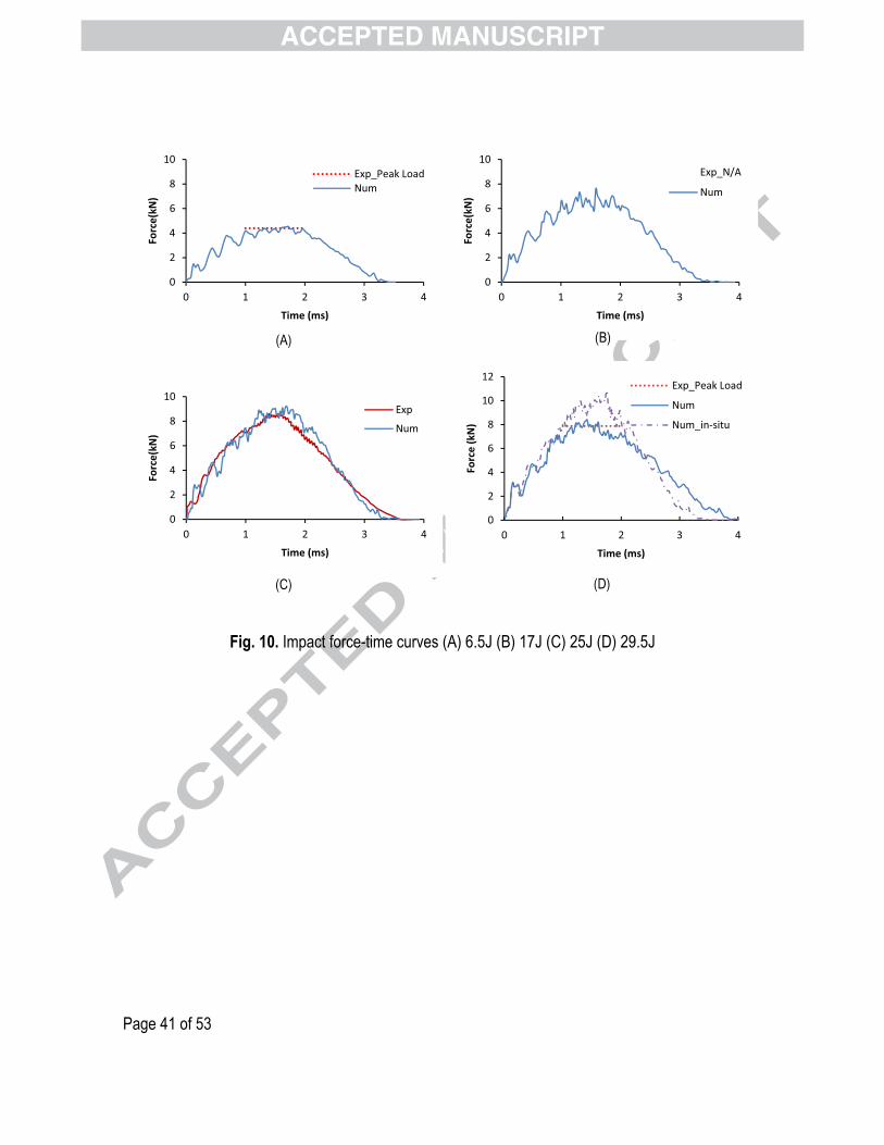
With reference to Figure 10, the extent of experimental data available varied between the tests

reported for different impact energies. For example, the complete history of the contact force of the impactor

versus time was only reported for the 25J impact on the panel manufactured from T700GC/M21 (Fig 10C).

This shows very good agreement, with the predicted maximum force being 6.8% higher than the one

measured experimentally. The predicted peak forces for the 6.5J (Fig 10A) and 29.5J (Fig 10D) impacts also

correlated well with experimental results, where the numerical peak loads were 3.2% and 6.7% higher than

experimental tests, respectively. No peak load information was reported for the 17J impact test but the

numerical impact-force versus time results are included for completeness.

Page 19 of 53

INSERT: Fig. 10. Impact force-time curves (A) 6.5J (B) 17J (C) 25J (D) 29.5J

The impact force-displacement histories in Fig. 11 (denoted by ‘Num’) correlate well with the

experimental results (denoted by ‘Exp’) recorded for the 6.5J (Fig. 11A), 25J (Fig. 11C) and 29.5J (Fig. 11D)

impact tests. The initial contact response, maximum displacements of the impactor and the rebound process

were all captured with good accuracy. It was observed that increasing the impact energy lead to a

corresponding increase in the maximum displacement and energy absorbed. The enclosed area within the

loading and unloading curves is a measure of the energy dissipated (or absorbed) due to damage in the

laminates. The dissipation energies, computed from the finite element analyses, were consistent with those

calculated from the change in kinetic energy of the impactor. Fig. 11E shows this change in energy for the four

test cases, where aE represents the energy absorbed during the 29.5J impact event. No force-displacement

data was available for the 17J impact case. Numerical results predicted that the 6.5J impact case would

absorb 2.35J, followed by 6.94J, 12.18J and 14.24J for impact energies 17J, 25J and 29.5J respectively.

INSERT: Fig. 11. Impact force-displacement curves (A) 6.5J (B) 17J (C) 25J (D) 29.5J and (E) Energy-

time curve

4.1.2 Matrix damage and delamination

Matrix cracking was found to be the dominant form of intralaminar failure for the range of impact

energies investigated, with little evidence of fibre breakage. Fig. 12 shows a superposition of intralaminar

matrix damage predicted by the damage model. Matrix cracking was concentrated around the impact region

with a symmetric and continuous distribution similar to that reported in [10]. The extent of matrix cracking is

shown to increase in proportion to the increase in impact energy.

INSERT: Fig. 12. Intralaminar matrix impact damage envelopes (A) 6.5J (B) 17J (C) 25J (D) 29.5J

Page 20 of 53

Delamination contours at each ply-pair interface were superimposed and compared to an outline of

C-Scan data obtained from reference [20] and presented in Fig. 13. Delaminations at the bottom 45°/0°

interface, for the 25J and 29.5J impact cases, tended to propagate along the 0° direction in the C-scan images

presented in [20] whereas the present analysis shows propagation predominantly along the 45° direction. The

C-scan contours for these two impact cases have been rotated to reflect this propagation preference. The

predicted delamination areas, listed in Fig. 13, show good agreement with the experimental/C-scan areas.

INSERT: Fig. 13. Delamination damage envelope compared with experimental C-scan outlines (A) 6.5J (B)

17J (C) 25J (D) 29.5J

Fig.14A shows matrix cracking and delamination for each double-ply and interface, respectively, for

the 29.5J impact case. Delaminations at each interface were deduced from the damage variable associated

with surface-based cohesive behaviour (through variable CSDMG).The shape and size of delaminations are

similar to the matrix damage areas except for the 90° plies which seem to show extensive damage extending

to the boundary. A similar observation was made in the damage model proposed by Raimondo et al.[10] but

no explanation was given. One possible explanation concerns the sensitivity to the relative strength and

toughness values used for interlaminar (delamination) and intralaminar matrix damage. For a given impact

energy, it has already been shown that excellent correlation was achieved in predicting the impactor force-time

and displacement-time histories, indicating that the overall energy dissipation is well predicted. Increasing the

damage initiation strength for intralaminar matrix damage, as shown in Fig 14B to explore in-situ effects and

discussed in more detail below, has a significant influence on the ratio of delamination to intralaminar matrix

damage. Fine-tuning these values through accurate material characterisation testing should yield a better

partition of these different matrix damage modes, whilst maintaining an accurate estimate of the overall energy

dissipation due to matrix damage. The maximum delaminated area occurred at the 45°/0° interface close to

Page 21 of 53

the bottom surface. The predicted intralaminar matrix damage envelopes followed the expected behaviour,

developing in the direction parallel to the fibre orientation.

The transverse tensile strength 60TY MPa= and shear strength 12 110S MPa= used in this

paper were not modified to account for in-situ effects although such effects were investigated and found to

yield comparatively poor results as discussed below. Dvorak and Laws [33] calculated the transition thickness

between a thin and a thick ply to be approximately 0.7mm for carbon/epoxy laminates. Since double plies were

modelled as one layer (0.52mm) in the simulation, the in-situ strength values were evaluated using the thin ply

equation presented by Camanho et al.[34] as an approximation,

,

221

22 11

497.4

1T is Ic

p

GY MPa

tE E

νπ= =

⎛ ⎞−⎜ ⎟⎝ ⎠

(34)

12

12

12

8193.98 , thin embedded ply

2 137.16 , thin outer ply

IIc

pis

IIc

p

G GMPa

tS

G GMPa

t

π

π

⎧=⎪

⎪= ⎨⎪ =⎪⎩

(35)

Where IcG and IIcG are the mode I and mode II fracture toughness, 12G is the shear modulus and pt is the

double-ply thickness. The overall effect of including in-situ effects is to raise the apparent respective strengths.

For simplicity, an average value of 12 165.57isS MPa= was used to represent the in-situ effect on shear

strength, and different intralaminar matrix damage and delamination contours were obtained (Fig.14B)

compared to those presented in Fig. 14A. Delamination become the major damage failure mode and

intralaminar matrix damage areas were comparatively smaller, especially noticeable in the 90° plies,

presumably since higher strengths made it more difficult to initiate intralaminar matrix damage. The smaller

area enclosed by the impact force-displacement curve, for the in-situ case, shown in Fig.11D, (denoted by

Page 22 of 53

‘Num_in-situ’) and the energy-time curve in Fig.16B, indicate less damage during the impact process. The

strength values obtained from standard tests, i,e, without in-situ modifications, yielded better predictions in

terms of the overall impact response, as can be seen in Fig.10D and Fig.11D. The influence of in-situ effects

requires a more detailed study which is beyond the scope of the work presented.

INSERT: Fig.14. Damage contours for plate impacted with 29.5J (A) Strength values of a ply (B) In-situ

strength values

4.1.4 Permanent indentation

The damage model has the capability of simulating the permanent indentation of composite laminates after the

impactor has rebounded and transient vibrations have subsided. Fig 15A shows an image of the permanent

indentation observed in the test while Fig 15B shows the out of-plane displacement contours from the analysis.

The permanent indentation captured by the model shows that the central indentation depth is approximately

0.7mm, which is in good agreement with experimental measurements [20]. The capability of the FE model to

capture permanent indentation is attributed to the nonlinear shear formulation of the intralaminar damage

model. This deformation may be significant in defining the compression-after-impact response of the laminates

[35]. As discussed in the formulation of the damage model, shear strain was decomposed into elastic strain

, ij elγ and inelastic strain , ij inγ components, the latter enabling the capture of post-impact indentation. The

energy dissipated by plasticity is given by Fig.15C, in which the inelastic energy is about one-third of the

overall energy dissipated by the damage.

INSERT: Fig. 15. Permanent indentation after impact (A) Experimental results (-0.7mm)[20]; (B) Numerical

results; (C) Energy dissipated by plasticity

Page 23 of 53

4.1.5 Energy dissipation mechanisms

As the impact event progresses, the energy absorbed by the laminates is mainly dissipated in the form of

intralaminar matrix damage, fibre-dominated damage, delamination, and impactor-laminate and ply–ply

friction. The absorbed energy of the laminate under an impact energy of 29.5J, and energy dissipated by each

damage mechanism is shown in Fig.16A as a function of time. Most of the energy is dissipated by intralaminar

matrix damage, which is consistent with the matrix-dominated damage envelope shown in Fig. 12D. The jump

in fibre-dominated energy dissipation indicates that this failure mode occurs suddenly during the impact

process. The total energy dissipated by these mechanisms almost equals the final energy absorbed of 14.24J,

calculated from the change in kinetic energy of the impactor and confirming the energy balance relationship.

The small discrepancy is due to the additional energy dissipated to control spurious zero energy modes which

may occur in reduced integration elements. A different trend is shown in Fig.16B, where the use of ‘in-situ’

transverse tensile and shear strengths reduced the energy absorbed to 8.7J and energy was mainly dissipated

by delamination.

INSERT: Fig. 16. Overall damage dissipation mechanism for 29.5J impact 29.5J (A) Standard strength values

of a ply (B) In-situ strength values

4.2 CAI Test

4.2.1 Stress-displacement curve

Applied stress versus end-displacement curves, obtained during CAI tests, show that excellent

correlation was achieved with experimental results, Fig. 17. The response of a pristine panel has been

included for comparison. For the 6.5J impact case, the effect on stiffness is minimal. This is to be expected as

impact-induced damage is not extensive. For the other cases, the reduction in stiffness is commensurate with

the level of impact damage. Compared to experimental results, the ultimate stresses were predicted to within

Page 24 of 53

10% of experiment results (7.7% for 6.5J, 9.2% for 17J, and 9.3% for 29.5J respectively). CAI data for the 25J

panel was not reported. Numerical results show that the damaged panels under 6.5J, 17J, 25J and 29.5J

impact energy failed at 10.1% , 28.4%, 45.9% and 54.2%, respectively, of the load carried by the pristine

panel. Fig. 17E represents the CAI strength versus impact energy for the tested laminates, which confirms the

high level of correlation achieved between experiment and numerical analysis.

INSERT: Fig. 17. CAI stress-displacement curves (A) 6.5J (B) 17J (C) 25J (D) 29.5J (E) CAI strength versus

impact energy

4.2.2 Intralaminar matrix damage

A sequence of superimposed intralaminar matrix damage maps at different displacement, obtained

from the virtual CAI test on the panel impacted with 29.5J, is shown in Fig. 18. The damage progression from

Fig18(A) to Fig18(D) indicated that matrix damage also initiated from the two outer edges, due to free-edge

effects, aligned with the central impacted region and propagated towards the damaged centre of the panel.

Local sub-laminate buckling, at the failure site, is observed in Fig. 18E, which indicates the presence of

extensive delamination (Fig. 21).

INSERT: Fig. 18. CAI matrix damage of 29.5J impact case at displacement of (A)0.6mm (B)0.65mm

(C)0.70mm (D)0.75mm (E) Side View

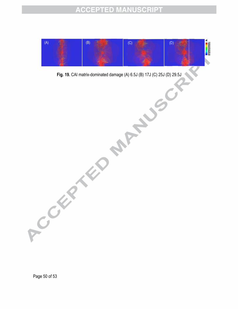
The superimposed intralaminar matrix damage contours for all panels, at ultimate failure, are shown in Fig. 19.

These confirm that damage propagated through the pre-damaged impacted centre of the panel which is

consistent with experimental observations [36].

Page 25 of 53

INSERT: Fig. 19. CAI Matrix-dominated Damage (A) 6.5J (B) 17J (C) 25J (D) 29.5J

4.2.3 Fibre-dominated damage

The final compressive fibre-dominated damage maps, from the virtual CAI tests, are shown in Fig. 20.

Complete fibre failure is observed through the width of the panel in the vicinity of the impact damage, with

most damage observed in the outer 0° plies and, to a lesser extent, in the ±45° plies. When the impact

damage is low (Fig. 20A), fibre breakage is observed through the impacted site, characterised by a single

dominant crack. As the energy increases, it is observed that multiple crack sites are predicted. This is

supported by some CAI tests [37] where these impacted sites, which are more heavily damaged, will

consequently shed more load into the neighbouring regions. This results in fibre breakage away from the

impact site where the high curvatures associated with sub-laminate buckling leads to further fibre damage.

INSERT: Fig. 20. Fibre failure (A) 6.5J (B) 17J (C) 25J (D) 29.5J

4.2.4 Overall damage and energy dissipation mechanisms

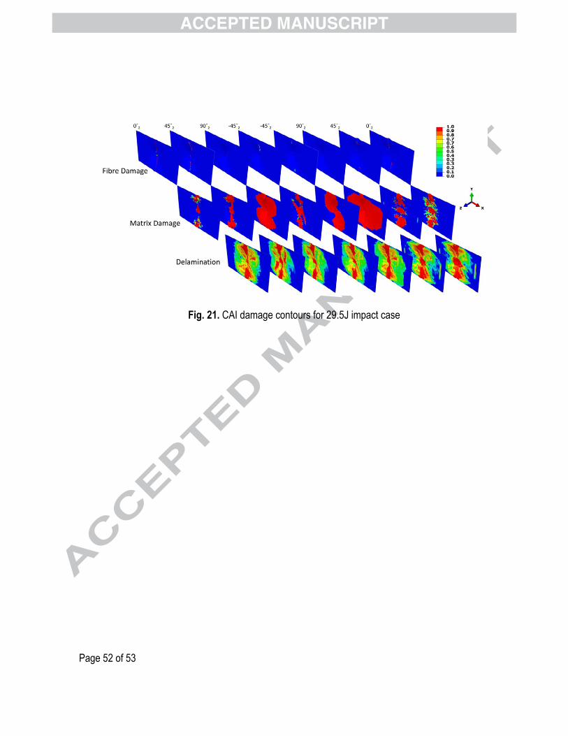
CAI damage plots for each ply pair and delaminations are shown in Fig.21 for the 29.5J impact case. During

the CAI process, new delamination and intralaminar matrix damage developed from the impact-induced

damage area. Fibre damage was primarily observed in the top and bottom plies. The predicted damage

correlated well with experimental findings.

INSERT: Fig. 21. CAI damage contours for 29.5J impact case

Page 26 of 53

The CAI energy dissipation curves in Fig.22 show that the rapid increase in fibre-dominated damage led to a

corresponding sudden load drop under displacement control. This failure mode was also associated with the

highest level of energy dissipation in comparison to the other damage mechanisms. This event was

accompanied by rapid increases in delamination and intralaminar matrix damage and moderate increases in

ply-to-ply friction.

INSERT: Fig. 22. CAI Energy dissipation curves for 29.5J impact case

5. Conclusions

A composite damage model that accounts for both intralaminar (matrix and fibre-dominated damage)

and interlaminar (delamination) damage was presented which has shown a high degree of capability in

predicting impact damage and compression-after-impact strength. This 3D model included an updated

damage initiation criterion, an accurate characteristic length determination, a robust unloading/reloading

mechanism and a unified matrix-dominated damage law.

The force-displacement curves, damage parameter maps and energy dissipated by each damage

mechanism, obtained from the numerical analysis, demonstrate that the model can capture both the qualitative

and quantitative aspects of intralaminar and interlaminar damage for a range of impact energies. Permanent

indentation was captured which may have a significant influence on the CAI response. The CAI simulations

predicted the complex damage features, and ensuing residual strength with a high degree of accuracy. This

was achieved without the need to calibrate the input parameters which were obtained from reliable literature

sources, following standard testing protocols. Future work will focus on extending this computational damage

model to capture high energy crush events which will enable accurate assessments of crashworthiness of

composite structures.

Page 27 of 53

Acknowledgement

The corresponding author would like to acknowledge the financial support of Bombardier and the Royal

Academy of Engineering. The authors would also like to gratefully acknowledge the funding from the Queen’s

University Belfast/China Scholarship Council (QUB/CSC) PhD Scholarship and the support from the Research

Computing Team at QUB in accessing the HPC facilities.

References

[1] Kachanov LM. Introduction to Continuum Damage Mechanics. Boston: Martinus Nijhoff Publishers. 1986. [2] Lemaitre J, Chaboche JL. Mechanics of solid materials. Cambridge, UK: Cambridge University Press; 1990. [3] Puck A, Schürmann H. Failure analysis of FRP laminates by means of physically based phenomenological models. Compos Sci Technol. 1998;58(7):1045-67. [4] Pinho S, Iannucci L, Robinson P. Physically based failure models and criteria for laminated fibre-reinforced composites with emphasis on fibre kinking. Part II: FE implementation. Composites Part A: Applied Science and Manufacturing. 2006;37(5):766-77. [5] Pinho S, Iannucci L, Robinson P. Physically-based failure models and criteria for laminated fibre-reinforced composites with emphasis on fibre kinking: Part I: Development. Composites Part A: Applied Science and Manufacturing. 2006;37(1):63-73. [6] Donadon MV, Iannucci L, Falzon BG, Hodgkinson JM, de Almeida SFM. A progressive failure model for composite laminates subjected to low velocity impact damage. Computers & Structures. 2008;86(11-12):1232-52. [7] Faggiani A, Falzon BG. Predicting low-velocity impact damage on a stiffened composite panel. Composites Part A: Applied Science and Manufacturing. 2010;41(6):737-49. [8] Falzon BG, Apruzzese P. Numerical analysis of intralaminar failure mechanisms in composite structures. Part I: FE implementation. Compos Struct. 2011;93(2):1039-46. [9] Falzon BG, Apruzzese P. Numerical analysis of intralaminar failure mechanisms in composite structures. Part II: Applications. Compos Struct. 2011;93(2):1047-53. [10] Raimondo L, Iannucci L, Robinson P, Curtis P. A progressive failure model for mesh-size-independent FE analysis of composite laminates subject to low-velocity impact damage. Compos Sci Technol. 2012;72(5):624-32. [11] Bouvet C, Rivallant S, Barrau JJ. Low velocity impact modeling in composite laminates capturing permanent indentation. Composites Science and Technology. 2012;72(16):1977-88.

Page 28 of 53

[12] Hongkarnjanakul N, Bouvet C, Rivallant S. Validation of low velocity impact modelling on different stacking sequences of CFRP laminates and influence of fibre failure. Composite Structures. 2013;106(0):549-59. [13] Uda N, Ono K, Kunoo K. Compression fatigue failure of CFRP laminates with impact damage. Composites Science and Technology. 2009;69(14):2308-14. [14] Ghelli D, Minak G. Low velocity impact and compression after impact tests on thin carbon/epoxy laminates. Composites Part B: Engineering. 2011;42(7):2067-79. [15] Petit S, Bouvet C, Bergerot A, Barrau J-J. Impact and compression after impact experimental study of a composite laminate with a cork thermal shield. Composites Science and Technology. 2007;67(15):3286-99. [16] Williams G, Bond I, Trask R. Compression after impact assessment of self-healing CFRP. Composites Part A: Applied Science and Manufacturing. 2009;40(9):1399-406. [17] Vieille B, Casado VM, Bouvet C. Influence of matrix toughness and ductility on the compression-after-impact behavior of woven-ply thermoplastic- and thermosetting-composites: A comparative study. Composite Structures. 2014;110(0):207-18. [18] Davies GAO, Hitchings D, Besant T, Clarke A, Morgan C. Compression after impact strength of composite sandwich panels. Composite Structures. 2004;63(1):1-9. [19] González E, Maimí P, Camanho P, Turon A, Mayugo J. Simulation of drop-weight impact and compression after impact tests on composite laminates. Composite Structures. 2012;94(11):3364-78. [20] Rivallant S, Bouvet C, Hongkarnjanakul N. Failure analysis of CFRP laminates subjected to compression after impact: FE simulation using discrete interface elements. Composites Part A: Applied Science and Manufacturing. 2013;55:83-93. [21] Chiu LN, Falzon BG, Boman R. A Continuum Damage Mechanics Model for the Analysis of the Crashworthiness of Composite Structures: A work in progress. Proceedings of the 15th Australian Aeronautical Conference. Melbourne2013. [22] Van Paepegem W, De Baere I, Lamkanfi E, Degrieck J. Monitoring quasi-static and cyclic fatigue damage in fibre-reinforced plastics by Poisson’s ratio evolution. International Journal of Fatigue. 2010;32(1):184-96. [23] Turon A, Camanho PP, Costa J, Davila CG. A damage model for the simulation of delamination in advanced composites under variable-mode loading. Mech Mater. 2006;38(11):1072-89. [24] Bažant ZP, Oh BH. Crack band theory for fracture of concrete. Matériaux et construction. 1983;16(3):155-77. [25] Catalanotti G, Camanho P, Marques A. Three-dimensional failure criteria for fiber-reinforced laminates. Compos Struct. 2012. [26] Press WH. Numerical recipes in Fortran 77: the art of scientific computing: Cambridge university press; 1992. [27] Systems D. ABAQUS Documentation 6.12. SIMULIA; 2012. [28] Benzeggagh ML, Kenane M. Measurement of mixed-mode delamination fracture toughness of unidirectional glass/epoxy composites with mixed-mode bending apparatus. Composites science and technology. 1996;56:439-49. [29] Prombut P, Michel L, Lachaud F, Barrau JJ. Delamination of multidirectional composite laminates at 0°/θ° ply interfaces. Engineering Fracture Mechanics. 2006;73(16):2427-42.

Page 29 of 53

[30] Turon A, Dávila CG, Camanho PP, Costa J. An engineering solution for mesh size effects in the simulation of delamination using cohesive zone models. Engineering Fracture Mechanics. 2007;74(10):1665-82. [31] Method AIT. Determination of Compression Strength after Impact. AITM 1-0010; 2010. [32] Preetamkumar M, Gilles L, Pierre L, Ana-cristina G. Validation of Intralaminar Behaviour of the Laminated Composites by Damage Mesomodel. 50th AIAA/ASME/ASCE/AHS/ASC Structures, Structural Dynamics, and Materials Conference: American Institute of Aeronautics and Astronautics; 2009. [33] Dvorak GJ, Laws N. Analysis of progressive matrix cracking in composite laminates II. First ply failure. Journal of Composite Materials. 1987;21(4):309-29. [34] Camanho PP, Dávila CG, Pinho ST, Iannucci L, Robinson P. Prediction of in situ strengths and matrix cracking in composites under transverse tension and in-plane shear. Composites Part A: Applied Science and Manufacturing. 2006;37(2):165-76. [35] Sztefek P, Olsson R. Nonlinear compressive stiffness in impacted composite laminates determined by an inverse method. Composites Part A: Applied Science and Manufacturing. 2009;40(3):260-72. [36] Yan H, Oskay C, Krishnan A, Xu LR. Compression-after-impact response of woven fiber-reinforced composites. Composites Science and Technology. 2010;70(14):2128-36. [37] Rivallant S, Bouvet C, Abi Abdallah E, Broll B, Barrau J-J. Experimental analysis of CFRP laminates subjected to compression after impact: The role of impact-induced cracks in failure. Composite Structures. 2014;111(0):147-57.

Figure captions

Fig. 1. Damage modes in laminated composites

Fig. 2. Bilinear law (shaded area is volumetric strain energy density)

Fig. 3. Material coordinate system (123) rotated to the fracture plane coordinate system (LNT)

Fig. 4. Non-linear shear curve with different loading/unloading paths

Fig. 5. Mixed-mode intralaminar matrix damage evolution

Fig. 6. Calculation of the characteristic length

Fig. 7. (A)DCB simulation with mesh size of 1.5mm (B) Load-displacement curve for different mesh

densities

Fig. 8. (A)ENF simulation with mesh size of 1.5mm (B) Load-displacement curve for different mesh densities

Fig. 9. (A) Impact and (B) CAI test setup

Page 30 of 53

Fig. 10. Impact force-time curves (A) 6.5J (B) 17J (C) 25J (D) 29.5J

Fig. 11. Impact force-displacement curves (A) 6.5J (B) 17J (C) 25J (D) 29.5J (E) energy-time curve

Fig. 12. Intralaminar matrix impact damage envelope (A) 6.5J (B) 17J (C) 25J (D) 29.5J

Fig. 13. Delamination damage envelope compared with experimental C-scan outline (dash line) (A) 6.5J (B)

17J (C) 25J (D) 29.5J

Fig. 14. Damage contours for plate impacted with 29.5J (A) Standard strength values of a ply (B) In-situ

strength values

Fig. 15. Permanent indentation after impact (A) Experimental results (-0.7mm)[20]; (B) Numerical results;

(C) Energy dissipated by plasticity

Fig. 16. Overall damage dissipation mechanism for 29.5J impact (A) Standard strength values of a ply (B) In-

situ strength values

Fig. 17. CAI stress-displacement curves (A) 6.5J (B) 17J (C) 25J (D) 29.5J (E) CAI Strength versus impact

energy

Fig. 18. CAI matrix damage of 29.5J impact case at displacement of (A)0.6mm (B)0.65mm (C)0.70mm

(D)0.75mm (E) Side View

Fig. 19. CAI matrix-dominated damage (A) 6.5J (B) 17J (C) 25J (D) 29.5J

Fig. 20. Fibre failure (A) 6.5J (B) 17J (C) 25J (D) 29.5J

Fig. 21. CAI damage contours for 29.5J impact case

Fig. 22. CAI energy dissipation curves for 29.5J impact case

Table 1. Material Properties of T700/M21 for numerical simulation [20, 12]

Property Values

Elastic Properties 1E 130GPa= ; 2 3 E E 7.7GPa= = ; 23G 3.8 ;GPa=

12 13G G 4.8GPa= = ; 12 13ν ν 0.3(0.33 )a= = ; 23ν 0.35=

Strength

TX 2080MPa= ;C X 1250MPa= ;

TY 60 ;MPa= CY 120 ;MPa= 12S 110MPa=

Intralaminar Fracture Toughness T11Γ 133 /N mm= ; ( )C

11Γ 10 40 /a N mm= ;

Page 31 of 53

( )T22Γ 0.5 0.6 /a N mm= ; ( )C

22Γ 1.6 2.1 /a N mm= ;

( )12 23 13Γ Γ Γ 1.6 2.1 /a N mm= = = ;

Non-linear Shear Properties 1c 37833MPa= ; 2 c 16512MPa= ; 3 c 2334.3MPa=

Interface Properties ( )0.5 0.6 /a

ICG N mm= ; ( )1.6 2.1 /aIICG N mm= ;

1.45η = ; 03 20MPaτ = ;

0 36sh MPaτ =

a Material : T700GC/M21 [12]

Pagge 332 oof 533

Figg. 1.. Da

amaage

F

mo

FIG

odes

GUR

s in

RES

lamminaatedd compoosittes

Pagge 333 oof 53

F

3

Fig. 2. Bili

inea

ar laaw ((sha

adedd arrea is v

volu

metric straain eneergy

y deensitty, )

Pag

Fig

ge 3

. 3.

34 o

Ma

of 53

ateri

3

ial ccoorrdinate sysstemm (1123)) rottateed to

o thhe frracture plaane cooordin

natee syysteem ((LNTT)

Pagge 335 oof 533

FFig. 4. Nonn-linnear

r shhearr curve with diifferrentt loaadinng/unloaadin

ng ppathhs

Pagge 336 oof 533

FFig. 5. MMixeed-m

modde intraalammina

ar mmatrrix ddammagee evvoluutionn

Pagge 3

37 oof 533

Fiig. 66. CCalcculationn of

the

(A

cha

A)

araccterristicc length

Page 38 of 53

(B)

Fig. 7. (A)DCB simulation with mesh size of 1.5mm (B) Load-displacement curve for different mesh

densities

0

10

20

30

40

50

60

70

80

90

100

0 1 2 3 4 5 6

Loa

d (

N)

Displacement (mm)

Anaytical

40 MPa &

Le=1.5mm

Page 39 of 53

(A)

(B)

Fig. 8. (A)ENF simulation with mesh size of 1.5mm (B) Load-displacement curve for different mesh

densities

0

100

200

300

400

500

600

700

800

0 2 4 6 8 10 12

Loa

d (

N)

Displacement (mm)

Analytical

40 MPa & Le=1.5mm

80 MPa & Le=0.3mm

Pagge 440 oof 533

(AA)

Figg. 9

9. (AA) Immpaact a

and (B)) CA

(B)

AI teest ssetuup

Page 41 of 53

Fig. 10. Impact force-time curves (A) 6.5J (B) 17J (C) 25J (D) 29.5J

0

2

4

6

8

10

0 1 2 3 4

Fo

rce

(kN

)

Time (ms)

Exp_Peak Load

Num

0

2

4

6

8

10

0 1 2 3 4

Fo

rce

(kN

)

Time (ms)

Exp_N/A

Num

0

2

4

6

8

10

0 1 2 3 4

Fo

rce

(kN

)

Time (ms)

Exp

Num

0

2

4

6

8

10

12

0 1 2 3 4

Fo

rce

(k

N)

Time (ms)

Exp_Peak Load

Num

Num_in-situ

(A) (B)

(C) (D)

Page 42 of 53

Fig. 11. Impact force-displacement curves (A) 6.5J (B) 17J (C) 25J (D) 29.5J (E) energy-time

curve

0

2

4

6

8

10

0 1 2 3 4 5 6

Fo

rce

(k

N)

Displacement (mm)

Exp

Num

0

2

4

6

8

10

0 1 2 3 4 5 6

Fo

rce

(k

N)

Displacement (mm)

Num

0

2

4

6

8

10

0 1 2 3 4 5 6

Fo

rce

(k

N)

Displacement (mm)

Exp

Num

0

2

4

6

8

10

12

0 1 2 3 4 5 6

Fo

rce

(k

N)

Displacement (mm)

Exp

Num

Num_in-situ

0

10

20

30

0 1 2 3 4

En

eg

y(J

)

Time (ms)

6.5J 17J 25J 29.5J

Exp N/A

(A) (B)

(C) (D)

��

(E)

Page 43 of 53

Fig. 12. Intralaminar matrix impact damage envelopes (A) 6.5J (B) 17J (C) 25J (D) 29.5J

(A) (B)

(C) (D)

Page 44 of 53

Fig. 13. Delamination damage envelope compared with experimental C-scan outlines (dashed lines)

(A) 6.5J (B) 17J (C) 25J (D) 29.5J

(C) (D)

(A) (B)

Exp=312.3mm2 Num=358.1mm2 Exp=1183.5mm2 Num=1117.8mm2

Exp=1442.6mm2 Num=1595.2mm2 Exp=1918.1mm2 Num=2097.2mm2

Page 45 of 53

(A)

(B)

Fig. 14. Damage contours for plate impacted with 29.5J (A) Standard strength values of a ply (B) In-

situ strength values

Page 46 of 53

(A) (B)

(C)

Fig. 15. Permanent indentation after impact (A) Experimental results (-0.7mm)[20]; (B) Numerical

results; (C) Energy dissipated by plasticity

0

1

2

3

4

5

6

7

0 1 2 3 4

En

erg

y (

J)

Time (ms)

Matrix Damage plasticity

Page 47 of 53

(A)

(B)

Fig. 16. Overall damage dissipation mechanism for 29.5J impact (A) Standard strength values of a

ply (B) In-situ strength values

0

5

10

15

20

25

30

35

0 1 2 3 4

En

erg

y (

J)

Time (ms)

Absorbed Energy Matrix Damage

Fibre Damage Delamination

Friction Energy Summation

0

5

10

15

20

25

30

35

0 1 2 3 4

En

erg

y (

J)

Time (ms)

Absorbed Delamination

Friction Matrix Damage

Energy Summation

Page 48 of 53

Fig. 17. CAI stress-displacement curves (A) 6.5J (B) 17J (C) 25J (D) 29.5J (E) CAI strength versus

impact energy

0

100

200

300

400

0 0.5 1 1.5

Str

ess

(MP

a)

Displacement (mm)

Undamaged Exp Num

0

100

200

300

400

0 0.5 1 1.5

Str

ess

(MP

a)

Displacement (mm)

Undamaged Exp Num

0

100

200

300

400

0 0.5 1 1.5

Str

ess

(MP

a)

Displacement (mm)

Undamaged Num

0

100

200

300

400

0 0.5 1 1.5

Str

ess

(MP

a)

Displacement (mm)

Undamaged Exp Num

0

100

200

300

400

0 5 10 15 20 25 30

Re

suid

al

Str

en

gth

(M

pa

)

Impact Energy (J)

Num

Exp

(A) (B)

(C) (D)

(E)

Pag

(A

ge 4

(C

A)

(E

49 o

Fi

C)0.7

(A)

E)

of 53

g. 1

70m

3

18. C

mm

CAI

(D)

I ma

0.7

atrix

5mm

x da

m (E

ama

E) S

(B

age

Side

)

of 2

e Vi

29.5

ew

5J im

mpaact ccasee at

(C)

t dissplaacemmennt off (AA)0.6

(D

6mm

D)

m (BB)0.65mmm

Pagge 5

(A

50 o

(A)

A)

of 533

Figg. 19. CCAI maatrix

(B

(B)

x-do

)

minnateed damage

e (A

(C

A) 6.

(C)

C)

5J ((B) 17JJ (CC) 255J ((D) 2

(D

(D)

29.5

D)

5J

Pagge 551 o

(A)

of 533

Figg. 200. F

(B

Fibre

B)

e failuree (AA) 6

.5J (B) 17J

(C)

J (CC) 25J ((D) 29.5J

(DD)

Page 52 of 53

Fig. 21. CAI damage contours for 29.5J impact case

Page 53 of 53

Fig. 22. CAI energy dissipation curves for 29.5J impact case

0

20

40

60

80

100

120

140

160

180

0

10

20

30

40

50

60

70

80

90

0 0.1 0.2 0.3 0.4 0.5 0.6 0.7 0.8 0.9

Str

ess

(MP

a)

En

erg

y (

J)

Displacement (mm)

Energy Absorbed Matrix

Fibre Delamination

Friction Load